Bayesian quantum phase estimation with fixed photon states
Abstract
We consider the generic form of a two-mode bosonic state with finite Fock expansion and fixed mean photon number to an integer . The upper and lower modes of the input state pick up a phase and respectively and we study the form of the optimal input state, i.e., the form of the state’s Fock coefficients, such that the mean square error (MSE) for estimating is minimized while the MSE is always attainable by a measurement. Our setting is Bayesian, meaning that we consider as a random variable that follows a prior probability distribution function (PDF). For the celebrated NOON state (equal superposition of and ), which is a special case of the input state we consider, and for a flat prior PDF we find that the Heisenberg scaling is lost and the attainable minimum mean square error (MMSE) is found to be , which is a manifestation of the fundamental difference between the Fisherian and Bayesian approaches. Then, our numerical analysis provides the optimal form of the generic input state for fixed values of and we provide evidence that a state produced by mixing a Fock state with vacuum in a beam-splitter of transmissivity (i.e. a special case of the state ), must correspond to . Finally, we consider an example of an adaptive technique: We consider a state of the form of for . We start with a flat prior PDF, and for each subsequent step we use as prior PDF the posterior probability of the previous step, while for each step we update the optimal state and optimal measurement. We show our analysis for up to five steps, but one can allow the algorithm to run further. Finally, we conjecture the form the of the prior PDF and the optimal state for the infinite step and we calculate the corresponding MMSE.
I Introduction
Quantum phase estimation is a field of study that has attracted the attention of the scientific community because of its high relevance to quantum technologies and its theoretical importance in studying quantum-enhanced sensing protocols by using non-classical phenomena such as squeezing and entanglement, which improve the scaling of the quantum Fisher information (QFI) Lane et al. (1993); Giovannetti et al. (2011); Pezzè et al. (2015); Crowley et al. (2014); Humphreys et al. (2013); Lang and Caves (2013).
The vast majority of the literature elaborates on and expands the knowledge of the Fisherian approach, i.e., when the estimated parameter has a fixed, yet unknown, value. In this approach, typically one engages with evaluating lower bounds on the mean squared error of an estimator. Said bounds are the well-known quantum and classical Cramér-Rao bounds, given by the inverse of the QFI and its classical counterpart, the classical Fisher information (CFI), aiming to show a quantum-enhancement of the sensing performance and to reveal the measurement that attains the quantum bound. Another direction to consider is the Bayesian setting: In this approach, the estimated parameter is considered as a random value that follows some probability distribution function (PDF), which is called the prior PDF. For single-variable Bayesian sensing tasks, exact formulas have been given for evaluating the minimum mean square error (MMSE), instead of lower bounding the MSE, in contrast to the Fisherian approach where the QFI serves as a lower bound to the Fisherian MSE. Said Bayesian MMSE is guaranteed to be always attainable by a measurement. In this paper we consider estimation of a single variable in the Bayasian approach, and specifically we consider the MMSE, not the Bayesian versions of the Cramér-Rao bound Van Trees et al. (2013); Gill and Levit (1995), on which notable works such as Jarzyna and Demkowicz-Dobrzański (2015); Morelli et al. (2021) have explored further. Moreover, it is worthwhile to note that multi-variable Bayesian lower bounds on the covariance matrix of an estimator have been established by minimizing the Bayesian MSE Rubio and Dunningham (2020); Sidhu and Kok (2020), while the conditions of their attainability are well-understood Rubio and Dunningham (2020); Sidhu and Kok (2020). Other notable works on precision bounds (Bayesian and more general than the Cramér-Rao bounds) include Tsang (2012); Lu and Tsang (2016); Rubio et al. (2018); Hall and Wiseman (2012).
Even though the mathematical setting for the Bayesian MMSE approach is known, compared to the QFI approach there are very few works exploiting it, some examples are Rubio and Dunningham (2019, 2020). As we note later in the paper and as already has been observed Zhou et al. (2023); Li et al. (2018), there is no direct correspondence between the Fisherian and the Bayesian approaches, as the two approaches assign different meaning to the concept of probability Li et al. (2018). In fact as we point out in Section III.2, the sensing performance can be significantly different than expected. Therefore, studying the quantum Bayesian sensing (QBS) is beneficial for two main reasons: It can give new results that may not be predicted by a Fisherian approach (or any Bayesian bounds build upon their Fisherian counterparts), which in turn will help to develop new intuition on Bayesian sensing, and it is a natural setting for adaptive techniques Morelli et al. (2021); Rubio et al. (2018); Rubio and Dunningham (2019); Lee et al. (2022); Wiebe and Granade (2016). In this paper, we consider a single phase as our unknown variable, therefore our analytic and numerical calculations pertain to the actual MMSE, not to a lower bound on the MSE.
The structure and main results of this work are: In Section II we explain our physical setting and we briefly give the mathematical tools we utilize. In Section III we compute the MMSE for the generic state, whose mean photon number is fixed to , for a flat prior PDF. Then, we consider two important special cases: a NOON state and the beam splitter generated state. For the former we derive results that when compared to their Fisherian counterparts are counter-intuitive. Lastly, we optimize all the MMSEs we computed over the input state. In Section IV we fix and we give a fully-optimized example of an adaptive phase sensing technique based on the Bayesian approach: Starting with a flat prior PDF and the corresponding optimal state, we update the prior PDF, the optimal input state, and the optimal measurement, for each sequential steps. Finally, in Section V we discuss our results and further research directions.
II The setting
Let the estimated single-variable to be , which in our case represents a phase shifting. The Bayesian MSE is defined as Personick (1971),
| (1) |
where is the state that holds the parameter (i.e. the final state), is the prior PDF, and is a Hermitian operator whose eigenvectors represent the measurement that we utilize to acquire information on .
We note that the MSE as defined in Eq. (1) is equivalent to the (perhaps) most commonly used form,
| (2) |
where , and are respectively the eigenvectors and eigenvalues of . If the spectrum of is continuous, the index is replaced by and the summation over by an integral over . The equivalence of Eqs. (1) and (2) can be shown be starting from Eq. (1) and writing the operator in its diagonal form.
Using Eq. (1) it has been shown Personick (1971) that minimizing over all possible , i.e., by solving the functional minimization problem,
| (3) |
we get the MMSE,
| (4) |
where,
| (5) |
and
| (6) |
where the MMSE is always attainable by the optimal projective measurement which is given by the eigenvectors of . We note here that is not in general unique, however any other possible optimal Hermitian , such that will result to the same for any given sensing task. This is proven by following the same reasoning for the QFI-based work Shi and Lu (2023).
In this work, we consider states whose Fock basis expansion has the form,
| (7) |
The mean photon number of such states is always regardless of the values of the complex coefficients which satisfy,
| (8) |
The phase sensing performance, within the Fisherian framework, of states in the form of Eq. (7) has been examined in Dorner et al. (2009) where it was proven to be significantly improved compared to classical interferometers.
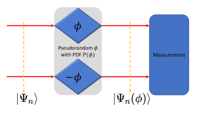
In our setting (see Fig. 1), the upper and lower modes of the input state pick up a phase and respectively, resulting to the output state,
| (9) |
Our immediate tasks entail to compute of Eq. (4) for and for the flat prior PDF,
| (10) |
which represents minimal prior knowledge Kołodyński and Demkowicz-Dobrzański (2010); Demkowicz-Dobrzański (2011), as opposed to a Dirac delta prior PDF which renders the MMSE equal to zero, i.e., full information on has already been given in the form of prior PDF. The flat prior PDF is also a natural assumption to initiate an adaptive technique, i.e., since we know nothing on the parameter a priori, we assume that all values have the same probability to occur. Lastly, it can be the choice of an adversary who holds the phase and can manipulate in a way that does not favor some values over others.
III MMSE evaluations for the flat prior PDF
III.1 The generic state
The goal of this section is to evaluate Eq. (4) for the state of Eq. (9) and the flat prior PDF of Eq. (10). From Eq. (5) we find,
| (11) |
where,
| (12) |
which for is evaluated to,
| (13) | |||||
| (16) | |||||
| (19) |
where denotes the Kronecker delta.
We note that the lower branch of Eq. (19) is not necessary since we are interested only in the diagonal terms of (per Eq. (4) we only need the trace of ). In any case we have calculated said lower branch for cross-checking reasons and for completeness. In fact we find,
| (20) |
From Eqs. (11) and (13) we find,
| (21) |
from which, since is diagonal on the Fock basis, we readily find,
| (22) |
From Eqs. (6), (11) (for ), (16), (22), and by paying attention that and do not commute, the second term of Eq. (4) gives,
| (23) |
Finally, from Eqs. (4), (20) and (23) we find the MMSE,
| (24) |
We note that the MMSE depends only the modulo of the complex coefficients . The choice of the flat prior PDF surely played a role in that; as we will see in Section IV, the choice of other prior PDFs does not result to such feature.
The optimal projective measurement is given by the eigenvectors of , a calculation that in principle is doable (analytically or numerically) since the matrix representation of said operator is finite. In Section IV we do an example for .
III.2 The NOON state
The NOON state,
| (25) |
where , is a special case of the state given in Eq. (7), i.e., for , Eq. (7) gives Eq. (25). We now consider the NOON state as the input state of Fig. 1 and the flat prior PDF of Eq. (10). Applying Eq. (24) we get the MMSE,
| (26) |
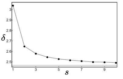
The MMSE of Eq. (26), albeit positive (it attains its minimal value for ), is a manifestation of the fundamental difference between the Bayesian and Fisherian approaches. Equation (26) increases monotonically with , while its Fisherian counterpart, i.e., the QFI (since we consider a single parameter, the QFI can be equal to a CFI Braunstein and Caves (1994)), scales as Dorner et al. (2009), i.e., , with a positive coefficient, in contrast to the negative coefficient of in Eq. (26). In Rubio and Dunningham (2020), the equivalent of Eq. (26), behaves as because the prior PDF therein depends on .
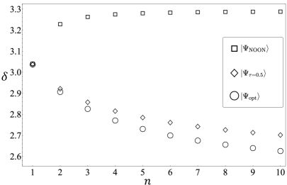
Lastly, we note that since for the flat prior PDF, Eq. (24) depends only on the absolute values of the coefficients , the MMSE of Eq. (26) will remain invariant even if we assume that the non-zero Fock coefficients of the NOON state have an imaginary part, while their absolute value is always equal to . We plot Eq. (26) as function of in Fig. 2.
In Appendix A we provide some further computations concerning truncated versions of the flat prior and the NOON state.
III.3 The beam splitter generated state
A way to construct a state in the form of Eq. (7), is to let the product state consisting of a Fock state and vacuum as input (upper and lower modes respectively) to a beam splitter of transmissivity , i.e.,
| (27) |
In this work we define the action of the beam splitter in the Heisenberg picture as,
| (28) |
where () are the input (output) annihilation operators and counts the modes starting from the top of Fig. 1. We find,
| (29) |
where,
| (30) |
Substituting the coefficnts of Eq. (30) into Eq. (24), we can obtain the expression of the MMSE for a flat prior PDF and the input state of Eq. (29). We note that if the coefficients are multiplied by a phase , the MMSE will remain invariant.
We ran numerical optimization (minimization) over of the MMSE of Eq. (24) using the coefficients of Eq. (30) (i.e. ) and for the flat prior PDF. Our constraints are: , , while the mean-photon number constraint comes natural since the state of Eq. (7) has a fixed photon number equal to . We considered values and we found the optimal value to be , resulting to the optimal beam splitter generated input state,
| (31) |
We plot the MMSE for said case in Fig. 2.
III.4 State optimization
We numerically find the optimal MMSE for the generic fixed photon number input state of Eq. (7) for . For said task, since the MMSE depends only on the absolute values of , we will assume (only up to the end of this section) that . Our constraints are: , , while, just as in Section III.3, the photon number is fixed as per the form of Eq. (7).
In Fig. 2 we present said optimized MMSE, and how it compares with the MMSEs of the NOON state and the optimized beam splitter generated state. For the sake of brevity, in Table 1 we give the optimal values of for up to , but one can have the numerics run for , something that is demonstrated in Fig. 2.
| 1 | 3.03987 | 0.707107 | 0.707107 | / | / | / | / |
| 2 | 2.90943 | 0.55108 | 0.626595 | 0.55108 | / | / | / |
| 3 | 2.82860 | 0.453382 | 0.542627 | 0.542627 | 0.453382 | / | / |
| 4 | 2.77333 | 0.386101 | 0.474686 | 0.501197 | 0.474686 | 0.386101 | / |
| 5 | 2.73304 | 0.336767 | 0.420815 | 0.457715 | 0.457715 | 0.420815 | 0.336767 |
We close this section by noting that for the optimal coefficients of the generic state of Eq. (7) can be found analytically. For said case we find,
| (32) |
while the optimal coefficients (up to an arbitrary phase) are,
| (33) | |||||
| (34) |
which is identical to the NOON state for and to the beam splitter generated state for and .
IV Adaptive technique
For simplicity, we will use the notation and , where is the dual-rail qubit basis. Therefore, we write the states of Eqs. (7) and (9) respectively for as,
| (35) | |||||
| (36) |
The two-mode phase shifting operation of Fig. 1 now reads , where is the Pauli operator such as and .
All matrix and vector representations in this section are understood in the dual-rail qubit basis. The optimal projective measurement is given by the eigenvectors of the operator . Since we consider a phase estimation problem and we fix the input state to be of the form of Eq. (35), the dimensions of the matrix representation of on the dual-rail qubit basis, will always be for everything that we will discuss in this section. Therefore, any possible measurement will have two possible outcomes. For example, if we use the flat prior PDF, from Eqs. (6), (10), and (35) we get,
| (37) |
For the flat prior PDF we have shown that the for the optimal state corresponds to . Therefore, for said case from Eq. (37) we get,
| (38) |
whose eigenvectors are,
| (39) | |||||
| (40) |
and the corresponding eigenvalues are , .
Now let us return to the Bayesian adaptive protocol and discuss how we get from one step to the next. For each step , we denote the quantities of interest, i.e., the prior PDF, the optimal state, the operator (whose eigenvectors provide the optimal projective measurement), and the optimal (minimum) MMSE respectively as follows, , , , . We also denote the eigenvectors of as and , while the corresponding eigenvalues are and . The indices take values .
For the first step (), we define , rendering the optimal state equal to , i.e., the state of Eq. (35) with the optimal coefficients of Eqs. (33) and (34), equal to that of Eq. (38), and the optimal MMSE equal to that of Eq. (32).
The connection between any two sequential steps is given by Bayes rule,
| (41) |
and utilizing the conditional probability as the prior PDF of the subsequent step, i.e.,
| (42) |
Therefore, to find the prior PDF for step , we must compute the probability and to use the prior PDF of the previous step. To compute (of step ), we use Born’s rule which requires to find the eigenvectors of .
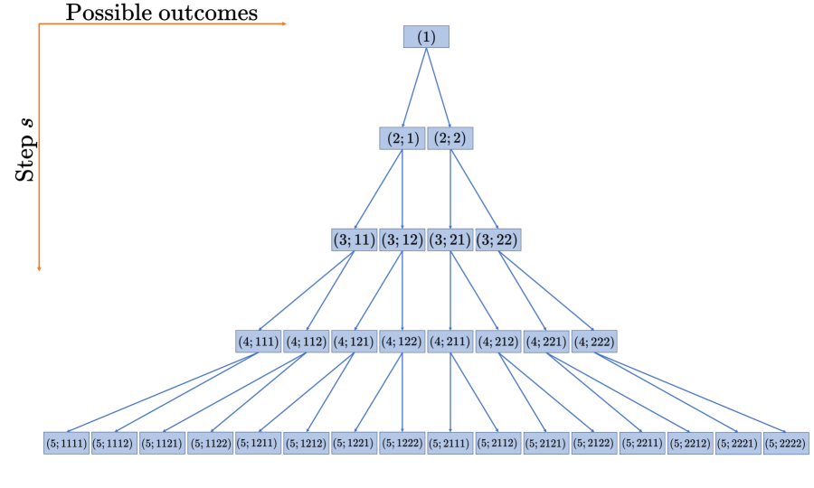
For step we have possible operators. To understand why, we consider the following example: Let , then we have one operator, that has two eigenvectors. Each one of the possible outcomes will correspond to a different probability, leading to a different prior PDF for the next step . Using these two prior PDF for step , we find two different operators. Then in step , each one of the aforesaid two operators will produce two possible measurement outcomes, i.e., four possible outcomes in total, and consequently four possible prior PDFs for the next step. For the same reason, for step we have in general different optimal states and optimal MMSEs, which are calculated using Eqs. (4), (5) and (6). The adaptive protocol is summarized in Fig. 3.
We have examined mostly numerically steps and all possible total possible quantities of interest. In Fig. 4 we present our findings: The optimal states and measurements for each step, i.e., those that correspond to the different prior PDFs, are not identical to each other, however all possible outcomes per step lead to the same optimized MMSE. As expected, the optimal state can always be written in the dual-rail qubit basis and in particular is always a phase shifted version of the state with which we initiated the adaptive protocol.
We demonstrate the evolution of the prior PDF in Fig. 5 for a specific path of Fig. 3, namely for the path that corresponds to the largest eigenvalue for each step (there is no physical reason for such choice, however it was computationally convenient to start with). We see that starting from a flat prior, after every step the prior PDF becomes sharper and taller, while the regions equal (or numerically close to) zero become more extended. That means, that the prior PDFs are becoming gradually more informative. Different downward paths in Fig. 3 give similar results.
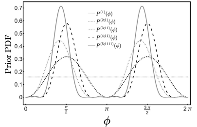
Assuming that the optimized MMSE will continue to be the same regardless of the different prior PDF choices, we were able to easily allow . We see that as the prior PDF trends to a double Dirac delta function, whose two peaks are separated by . For that limiting case, the (analytically calculated) MMSE is,
| (43) |
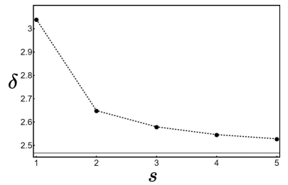
Under the last assumption, in Fig. 6 we show the optimized MMSE per step for up to .
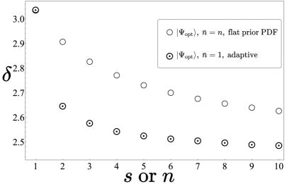
We now fix the total mean photon number that is available to the whole sensing protocol to be . Let us compare two strategies: (i) The adaptive strategy of this section, and (ii) the case of Section III.1, where we optimized the generic state. For the strategy (i), since we the mean photon number of the optimized state for each step is , the mean photon number that has been used up to step is . For strategy (ii) we have optimized the input state for all with , therefore for this non-adaptive, single-state-use case we have. The comparison is done by setting and we ask whether is better to apply our adaptive protocol or use the whole mean photon number budget in one go using the optimal state with and the flat prior PDF. We show our results in Fig. 7, where we see that the MMSE of strategy (i) is less than the MMSE of strategy (ii) for the some mean photon budget, i.e., the adaptive technique is superior to the non-adaptive one. The numerical simulations of this section can be found in Zhou and Gagatsos (2023).
V Conclusions
In this work we presented a genuine Bayesian phase sensing problem and we showed that the departure from the Fisherian approach is strongly manifested when using resources, i.e., NOON states, whose performance in the Fisherian domain is known to provide quantum-enhancement. However, such resource states fail to perform adequately in the Bayesian domain, at least for the flat prior PDF. Moreover, we optimized the general class of fixed-photon number states (NOON states is a sub-case thereof) to re-establish an at least decreasing behavior of the Bayesian MMSE, and we investigated the case of states that can be produced using a Fock state, vacuum, and a beam-splitter.
Then we presented an adaptive protocol that takes into account all possible outcomes of the optimal measurement per step, giving rise to the tree diagram of Fig. 3. Our optimization over all possible paths gives the MMSE (as function of the step ) regardless of the path we choose.
Within the Bayesian lines of thought we understand the adaptive technique in the subjective Bayesian fashion. The sensor (who controls the input states and the measurements) updates their personal, potentially subjective, belief (i.e. the prior PDF) utilizing a sequence of optimal measurements. Of course, the target (who holds and controls the unknown variable), cannot be affected by the conclusions of the sensor. However, sensor and target might either agree beforehand on a starting prior PDF or the sensor might be somewhat informed on the target’s behavior. Then, the sensor is doing their best to enhance their precision, which leads to a purely instrumentalist interpretation of any prior PDF for steps : It is merely the mathematical means to enhance the sensing performance, and not a reality on the target’s side. Non attaining an MMSE , i.e., something that could happen for the Dirac delta prior PDF for some ultimate step, but instead attaining a double Dirac delta, as our analysis suggests, is the price to pay for trying to estimate a random variable and assigning the specific initial prior PDF. Whoever, in accordance to objective Bayesian statistics one must assign weakly-informative prior PDFs, which heuristically leads to the use of the flat prior PDF. Then, any updates on this, are the best thing that can happen, since said updates are based on optimal measurements.
We note that we strictly work on sensing a random variable, which is not necessarily a fixed parameter whose value is just unknown to the sensor. If the case was the latter we would anticipate that the MMSE would eventually go (close) to zero, and not to the value of Eq. (43).
Further research opportunities on the general subject of present work are surfacing: It could be worthwhile to examine multi-mode and/or multi-variable systems with any combination of non-classical, Gaussian, and entangled states, aiming to reveal the optimal choices for given sensing tasks. Departing from works (like the current one) that are concerned with fundamentally optimal behavior, it would be interesting to expand the analysis to systems suffering losses and noise.
Acknowledgements.
The authors acknowledge useful discussions with Boulat Bash (University of Arizona). B.Z. acknowledges financial support from C.N.G.’s start-up fund (University of Arizona, ECE department). B.Z. and S.G. acknowledge the DARPA IAMBIC Program funded under Contract No. HR00112090128.Appendix A MMSE for a truncated flat prior
In this Appendix we consider as input sate the NOON state of Eq. (25) and the truncated version of the flat prior as the prior PDF,
| (A1) |
where the parameter controls the size of the truncated length (i.e. for , Eq. (A1) gives Eq. (10) that we used in the main text).
For said case we calculate the expression of the MMSE. Using Eq. (5), we get,
| (A4) |
where is the incomplete Gamma function. From Eqs. (6), (4) and (A4), we can get the MMSE for the NOON input state and the truncated flat prior,
| (A5) |
We note that for , since is always an integer, and , Eq. (A5) gives Eq. (26).
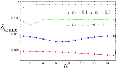
The role of parameter is shown in Fig. A1. The MMSE becomes smaller as becomes smaller. This is because when decreases, we eliminate the range of . So we have more information about the unknown variable . When photon number is not large, the MMSE will first decrease as increases. After the MMSE reaches the minimal value at a specific , the MMSE will start increasing again. For , although we can only see the downtrend, however (not shown in Fig. A1, but can verified analytically from Eq. (A5)) it will start increasing at around . Similarly for smaller .
References
- Lane et al. (1993) Alistair S. Lane, Samuel L. Braunstein, and Carlton M. Caves, “Maximum-likelihood statistics of multiple quantum phase measurements,” Phys. Rev. A 47, 1667–1696 (1993).
- Giovannetti et al. (2011) Vittorio Giovannetti, Seth Lloyd, and Lorenzo Maccone, “Advances in quantum metrology,” Nature Photonics 5, 222–229 (2011).
- Pezzè et al. (2015) Luca Pezzè, Philipp Hyllus, and Augusto Smerzi, “Phase-sensitivity bounds for two-mode interferometers,” Phys. Rev. A 91, 032103 (2015).
- Crowley et al. (2014) Philip J. D. Crowley, Animesh Datta, Marco Barbieri, and I. A. Walmsley, “Tradeoff in simultaneous quantum-limited phase and loss estimation in interferometry,” Phys. Rev. A 89, 023845 (2014).
- Humphreys et al. (2013) Peter C. Humphreys, Marco Barbieri, Animesh Datta, and Ian A. Walmsley, “Quantum enhanced multiple phase estimation,” Phys. Rev. Lett. 111, 070403 (2013).
- Lang and Caves (2013) Matthias D. Lang and Carlton M. Caves, “Optimal quantum-enhanced interferometry using a laser power source,” Phys. Rev. Lett. 111, 173601 (2013).
- Van Trees et al. (2013) Harry L Van Trees, Kristine L Bell, and Zhi Tian, Detection estimation and modulation theory, part I, 2nd ed. (Wiley-Blackwell, Hoboken, NJ, 2013).
- Gill and Levit (1995) Richard D. Gill and Boris Y. Levit, “Applications of the van trees inequality: A bayesian cramér-rao bound,” Bernoulli 1, 59–79 (1995).
- Jarzyna and Demkowicz-Dobrzański (2015) Marcin Jarzyna and Rafał Demkowicz-Dobrzański, “True precision limits in quantum metrology,” New Journal of Physics 17, 013010 (2015).
- Morelli et al. (2021) Simon Morelli, Ayaka Usui, Elizabeth Agudelo, and Nicolai Friis, “Bayesian parameter estimation using gaussian states and measurements,” Quantum Science and Technology 6, 025018 (2021).
- Rubio and Dunningham (2020) Jesús Rubio and Jacob Dunningham, “Bayesian multiparameter quantum metrology with limited data,” Phys. Rev. A 101, 032114 (2020).
- Sidhu and Kok (2020) Jasminder S. Sidhu and Pieter Kok, “Geometric perspective on quantum parameter estimation,” AVS Quantum Science 2, 014701 (2020).
- Tsang (2012) Mankei Tsang, “Ziv-zakai error bounds for quantum parameter estimation,” Phys. Rev. Lett. 108, 230401 (2012).
- Lu and Tsang (2016) Xiao-Ming Lu and Mankei Tsang, “Quantum weiss-weinstein bounds for quantum metrology,” Quantum Science and Technology 1, 015002 (2016).
- Rubio et al. (2018) Jesús Rubio, Paul Knott, and Jacob Dunningham, “Non-asymptotic analysis of quantum metrology protocols beyond the cramér–rao bound,” Journal of Physics Communications 2, 015027 (2018).
- Hall and Wiseman (2012) Michael J W Hall and Howard M Wiseman, “Heisenberg-style bounds for arbitrary estimates of shift parameters including prior information,” New Journal of Physics 14, 033040 (2012).
- Rubio and Dunningham (2019) Jesús Rubio and Jacob Dunningham, “Quantum metrology in the presence of limited data,” New Journal of Physics 21, 043037 (2019).
- Zhou et al. (2023) Boyu Zhou, Boulat A. Bash, Saikat Guha, and Christos N. Gagatsos, “Bayesian minimum mean square error for transmissivity sensing,” (2023), arXiv:2304.05539 [quant-ph] .
- Li et al. (2018) Yan Li, Luca Pezzè, Manuel Gessner, Zhihong Ren, Weidong Li, and Augusto Smerzi, “Frequentist and bayesian quantum phase estimation,” Entropy 20 (2018), 10.3390/e20090628.
- Lee et al. (2022) Kwan Kit Lee, Christos N. Gagatsos, Saikat Guha, and Amit Ashok, “Quantum-inspired multi-parameter adaptive bayesian estimation for sensing and imaging,” IEEE Journal of Selected Topics in Signal Processing , 1–11 (2022).
- Wiebe and Granade (2016) Nathan Wiebe and Chris Granade, “Efficient bayesian phase estimation,” Phys. Rev. Lett. 117, 010503 (2016).
- Personick (1971) S. Personick, “Application of quantum estimation theory to analog communication over quantum channels,” IEEE Transactions on Information Theory 17, 240–246 (1971).
- Shi and Lu (2023) Yingying Shi and Xiao-Ming Lu, “Joint optimal measurement for locating two incoherent optical point sources near the rayleigh distance,” Communications in Theoretical Physics 75, 045102 (2023).
- Dorner et al. (2009) U. Dorner, R. Demkowicz-Dobrzanski, B. J. Smith, J. S. Lundeen, W. Wasilewski, K. Banaszek, and I. A. Walmsley, “Optimal quantum phase estimation,” Phys. Rev. Lett. 102, 040403 (2009).
- Kołodyński and Demkowicz-Dobrzański (2010) Jan Kołodyński and Rafał Demkowicz-Dobrzański, “Phase estimation without a priori phase knowledge in the presence of loss,” Phys. Rev. A 82, 053804 (2010).
- Demkowicz-Dobrzański (2011) Rafał Demkowicz-Dobrzański, “Optimal phase estimation with arbitrary a priori knowledge,” Phys. Rev. A 83, 061802 (2011).
- Braunstein and Caves (1994) Samuel L. Braunstein and Carlton M. Caves, “Statistical distance and the geometry of quantum states,” Phys. Rev. Lett. 72, 3439–3443 (1994).
- Zhou and Gagatsos (2023) Boyu Zhou and Christos Gagatsos, “Mathematica file for Bayesian Adaptive Method of Phase Sensing,” (2023), 10.25422/azu.data.23811177.v1.