On representations of the Helmholtz Green’s function

Abstract.

We consider the free space Helmholtz Green’s function and split it into the sum of oscillatory and non-oscillatory (singular) components. The goal is to separate the impact of the singularity of the real part at the origin from the oscillatory behavior controlled by the wave number $k$. The oscillatory component can be chosen to have any finite number of continuous derivatives at the origin and can be applied to a function in the Fourier space in $\mathcal{O}\left(k^{d}\log k\right)$ operations. The non-oscillatory component has a multiresolution representation via a linear combination of Gaussians and is applied efficiently in space.

Since the Helmholtz Green’s function can be viewed as a point source, this partitioning can be interpreted as a splitting into propagating and evanescent components. We show that the non-oscillatory component is significant only in the vicinity of the source at distances $\mathcal{O}\left(c_{1}k^{-1}+c_{2}k^{-1}\log_{10}k\right)$, for some constants $c_{1}$, $c_{2}$, whereas the propagating component can be observed at large distances.

1. Introduction

In this paper we consider the free space Helmholtz Green’s function given by

(1.1) $$G\left(r\right)=\left\{\begin{array}[]{rc}{\displaystyle\frac{1}{4\pi}\frac{e^{ikr}}{r}=\frac{1}{4\pi}\frac{\cos\left(kr\right)}{r}+\frac{i}{4\pi}\frac{\sin\left(kr\right)}{r}}&\mbox{in dimension }d=3,\\ \\ {\displaystyle\frac{i}{4}H_{0}^{(1)}\left(kr\right)=-\frac{1}{4}Y_{0}\left(kr\right)+\frac{i}{4}J_{0}\left(kr\right)}&\mbox{in dimension }d=2,\end{array}\right.$$

where $H_{0}^{(1)}$ is the Hankel function of the first kind, $J_{0}$ and $Y_{0}$ are the Bessel functions of the first and second kind, $r=\left\|\mathbf{x}\right\|=\left(\sum_{j=1}^{d}x_{j}^{2}\right)^{1/2}$ denotes the Euclidean norm of the vector $\mathbf{x}$ and $k>0$. We separate $G$ into the sum of oscillatory and non-oscillatory (singular) components. The oscillatory component can be chosen to have any finite number of continuous derivatives at $r=0$. As far as we know, previous approaches to split $G$ in this manner did not allow to choose the number of smooth derivatives at $r=0$. As in [6, 5], the oscillatory component can be applied to a function in the Fourier space in $\mathcal{O}\left(k^{d}\log k\right)$ operations. The non-oscillatory component has a multiresolution representation via a linear combination of Gaussians and is applied efficiently in space.

Our approach is a modification of that in [6, 5] leading to explicit formulas. The goal is to separate the impact of the singularity of the real part of (1.1) at the origin from the oscillatory behavior controlled by the wave number $k$. Specifically, we want the number of derivatives at the origin of the oscillatory component to be user selected and the non-oscillatory component to have a multiresolution representation via a linear combination of Gaussians. For non-oscillatory kernels integral representations involving Gaussians lead to efficient multiresolution approximations (see e.g. [16, 7, 3, 8, 9, 4, 15, 1]), i.e. when approaching a singularity the domain of integration automatically shrinks leading to fast algorithms for application of such kernels. We want a similar representation of the non-oscillatory component of the Helmholtz Green’s function (1.1).

Since $G$ in (1.1) can be interpreted as a point source, a physical interpretation of splitting it into oscillatory and non-oscillatory components may be viewed as a splitting into propagating and evanescent components. Indeed, we show that the non-oscillatory component is significant only in the vicinity of the source at distances $\mathcal{O}\left(c_{1}k^{-1}+c_{2}k^{-1}\log_{10}k\right)$, for constants $c_{1}$, $c_{2}$, whereas the propagating component can be observed at large distances.

2. Preliminaries

2.1. Green’s functions

The free space Green’s function (1.1) of the Helmholtz equation satisfies

(2.1) $$\Delta G\left(\mathbf{x}\right)+k^{2}G\left(\mathbf{x}\right)=-\delta\left(\mathbf{x}\right),$$

and, on taking the Fourier transform of (2.1), we obtain

(2.2) $$\widehat{G}\left(\left\|\mathbf{p}\right\|\right)=\frac{1}{\left\|\mathbf{p}\right\|^{2}-k^{2}},$$

where $\mathbf{p}\in\mathbb{R}^{d}$, $d=2,3$, We use the Fourier transform defined as

(2.3) $$\widehat{f}\left(\mathbf{p}\right)=\int_{\mathbb{R}^{d}}f\left(\mathbf{x}\right)e^{-i\mathbf{x}\cdot\mathbf{p}}d\mathbf{x}$$

and its inverse as

(2.4) $$f\left(\mathbf{x}\right)=\frac{1}{\left(2\pi\right)^{d}}\int_{\mathbb{R}^{d}}\widehat{f}\left(\mathbf{p}\right)e^{i\mathbf{x}\cdot\mathbf{p}}d\mathbf{p}.$$

The inverse Fourier transform of $\widehat{G}$ is a singular integral and we use regularization (see [6])

(2.5) $$G(\mathbf{x})=\lim_{\lambda\rightarrow 0^{+}}\frac{1}{(2\pi)^{d}}\int_{\mathbb{R}^{d}}\frac{e^{i\mathbf{x}\cdot\mathbf{p}}}{\left\|\mathbf{p}\right\|^{2}-\left(k+i\lambda\right)^{2}}d\mathbf{p},$$

which yields the outgoing Green’s functions (1.1) satisfying the Sommerfeld radiation condition

(2.6) $$\lim_{r\rightarrow\infty}r{}^{\frac{d-1}{2}}\left(\frac{\partial G}{\partial r}-ikG\right)=0.$$

Following [6], we define

$$\hat{G}_{\lambda}\left(p\right)=\frac{1}{p^{2}-\left(k+i\lambda\right)^{2}}=\frac{1}{2p}\left(\frac{1}{p-k-i\lambda}+\frac{1}{p+k+i\lambda}\right)$$

and separate its real and imaginary parts

(2.7) $$\mathcal{R}e\left(\hat{G}_{\lambda}\left(p\right)\right)=\frac{1}{2p}\left(\frac{p-k}{\left(p-k\right){}^{2}+\lambda^{2}}+\frac{p+k}{\left(p+k\right){}^{2}+\lambda^{2}}\right)$$

and

(2.8) $$\mathcal{I}m\left(\hat{G}_{\lambda}\left(p\right)\right)=\frac{1}{2p}\left(\frac{\lambda}{\left(p-k\right){}^{2}+\lambda^{2}}-\frac{\lambda}{\left(p+k\right){}^{2}+\lambda^{2}}\right).$$

We observe that the limit

(2.9) $$\lim_{\lambda\rightarrow 0^{+}}\mathcal{I}m\left(\hat{G}_{\lambda}\left(p\right)\right)=\frac{\pi}{2p}\left(\delta\left(p-k\right)-\delta\left(p+k\right)\right)$$

is a generalized function (see e.g. [10, Chapter III, section 1.3]) corresponding to integration over the sphere in the Fourier domain. Using e.g. [12, Section 4.1], we have

$$\lim_{\lambda\rightarrow 0^{+}}\int_{0}^{\infty}\frac{1}{2p}\left(\frac{p-k}{\left(p-k\right)^{2}+\lambda^{2}}+\frac{p+k}{\left(p+k\right){}^{2}+\lambda^{2}}\right)d\rho=\mbox{p.v.}\int_{0}^{\infty}\frac{1}{p^{2}-k^{2}}d\rho,$$

so that

(2.10) $$\mathcal{R}e\left(G\left(\mathbf{x}\right)\right)=\frac{1}{(2\pi)^{d}}\mbox{p.v.}\int_{\mathbb{R}^{d}}\frac{e^{i\mathbf{x}\cdot\mathbf{p}}}{\left\|\mathbf{p}\right\|^{2}-k^{2}}d\mathbf{p},$$

where the principal value is considered about $\left\|\mathbf{p}\right\|=k$.

3. Splitting of the Green’s function in the Fourier domain

We start with

Lemma 1.

For $n\geq 1$ and $p\neq k$ we have

(3.1) $$\frac{1}{p^{2}-k^{2}}-\widehat{g}_{n}\left(p,k\right)=\frac{1}{p^{2}-k^{2}}\frac{\left(2k^{2}\right)^{n}}{\left(p^{2}+k^{2}\right)^{n}}=\mathcal{O}\left(\frac{1}{p^{2n+2}}\right),$$

where

(3.2) $$\widehat{g}_{n}\left(p,k\right)=\sum_{j=0}^{n-1}\frac{\left(2k^{2}\right)^{j}}{\left(p^{2}+k^{2}\right)^{j+1}}.$$

Proof.

We have

$$\widehat{g}_{n}\left(p,k\right) = \frac{1}{p^{2}+k^{2}}\sum_{j=0}^{n-1}\frac{\left(2k^{2}\right)^{j}}{\left(p^{2}+k^{2}\right)^{j}}$$

$$= \frac{1}{p^{2}+k^{2}}\left(1-\frac{\left(2k^{2}\right)^{n}}{\left(p^{2}+k^{2}\right)^{n}}\right)\left(1-\frac{2k^{2}}{p^{2}+k^{2}}\right)^{-1}$$

$$= \frac{1}{p^{2}-k^{2}}\left(1-\frac{\left(2k^{2}\right)^{n}}{\left(p^{2}+k^{2}\right)^{n}}\right)$$

$$= \frac{1}{p^{2}-k^{2}}-\frac{1}{p^{2}-k^{2}}\frac{\left(2k^{2}\right)^{n}}{\left(p^{2}+k^{2}\right)^{n}}$$

and arrive at (3.1) as an algebraic identity for $p\neq k$. ∎

Using Lemma 1, we obtain the splitting of (2.2) in the Fourier domain as

(3.3) $$\widehat{G}\left(\left\|\mathbf{p}\right\|\right)=\widehat{g}_{n}\left(\left\|\mathbf{p}\right\|,k\right)+\widehat{g}_{n,oscill}\left(\left\|\mathbf{p}\right\|,k\right),$$

where

(3.4) $$\widehat{g}_{n,oscill}\left(\left\|\mathbf{p}\right\|,k\right)=\frac{1}{\left\|\mathbf{p}\right\|^{2}-k^{2}}\frac{\left(2k^{2}\right)^{n}}{\left(\left\|\mathbf{p}\right\|^{2}+k^{2}\right)^{n}}$$

and

(3.5) $$\widehat{g}_{n}\left(\left\|\mathbf{p}\right\|,k\right)=\sum_{j=0}^{n-1}\frac{\left(2k^{2}\right)^{j}}{\left(\left\|\mathbf{p}\right\|^{2}+k^{2}\right)^{j+1}}.$$

The rate of decay of $\widehat{g}_{n,oscill}$ in the Fourier domain for $\left\|\mathbf{p}\right\|>k$ is $\mathcal{O}\left(\left\|\mathbf{p}\right\|^{-2n-2}\right)$ so that the volume of its significant support is proportional to $k^{d}$. Following [6, 5], we have

$$\widehat{G}\left(\left\|\mathbf{p}\right\|\right)=\frac{1}{2\left\|\mathbf{p}\right\|}\left(\frac{1}{\left\|\mathbf{p}\right\|-k}+\frac{1}{\left\|\mathbf{p}\right\|+k}\right) =$$

$$\frac{1}{2\left\|\mathbf{p}\right\|}\int_{0}^{\infty}\left[\left(\left\|\mathbf{p}\right\|-k\right)e^{-s\left(\left\|\mathbf{p}\right\|-k\right)^{2}}+\left(\left\|\mathbf{p}\right\|+k\right)e^{-s\left(\left\|\mathbf{p}\right\|+k\right)^{2}}\right]ds$$

yielding

$$\widehat{g}_{n,oscill}\left(\left\|\mathbf{p}\right\|,k\right)=\frac{2^{n-1}k^{2n}}{\left(\left\|\mathbf{p}\right\|^{2}+k^{2}\right)^{n}}\frac{1}{\left\|\mathbf{p}\right\|}\int_{0}^{\infty}\left[\left(\left\|\mathbf{p}\right\|-k\right)e^{-s\left(\left\|\mathbf{p}\right\|-k\right)^{2}}+\left(\left\|\mathbf{p}\right\|+k\right)e^{-s\left(\left\|\mathbf{p}\right\|+k\right)^{2}}\right]ds,$$

or

(3.6) $$\widehat{g}_{n,oscill}\left(\left\|\mathbf{p}\right\|,k\right)=\frac{2^{n-1}k^{2n}}{\left(\left\|\mathbf{p}\right\|^{2}+k^{2}\right)^{n}}\frac{1}{\left\|\mathbf{p}\right\|}\int_{-\infty}^{\infty}\left[\left(\left\|\mathbf{p}\right\|-k\right)e^{-e^{t}\left(\left\|\mathbf{p}\right\|-k\right)^{2}}+\left(\left\|\mathbf{p}\right\|+k\right)e^{-e^{t}\left(\left\|\mathbf{p}\right\|+k\right)^{2}}\right]e^{t}dt,$$

where $\mathbf{p}\in\mathbb{R}^{d}$, $d=2,3$. The integral in (3.6) is a multiresolution representation of $\widehat{g}_{n,oscill}$ centered at the singularity $\left\|\mathbf{p}\right\|=k$. This representation allows us to implement the principal value limit (see e.g. (2.10)) by simply ignoring fine scales since, at some point, their contribution is negligible. Effectively it amounts to replacing the upper limit in the integral in (3.6) by a carefully chosen finite value. Discretizing (3.6) leads to an approximation of $\widehat{g}_{n,oscill}$ via a linear combination of smooth (rotationally invariant) kernels similar to that obtained in [6]. We refer to [6] for the details of applying $\widehat{g}_{n,oscill}$ to a function via an algorithm of complexity $\mathcal{O}\left(k^{d}\log k\right)$.

4. Spatial representations in $\mathbb{R}^{3}$

While the oscillatory component is applied efficiently in the Fourier domain due to its rapid decay, the non-oscillatory component decays slowly in the Fourier domain but its application is efficient in space. We start by computing spatial representations in $\mathbb{R}^{3}$ since these are different in dimensions $d=3$ and $d=2$.

Lemma 2.

The inverse Fourier transform of the non-oscillatory component (3.5) is given by

(4.1) $$g_{n}\left(r,k\right)=\frac{1}{4\pi}\frac{e^{-kr}}{r}\left(1+\sum_{j=1}^{n-1}\frac{1}{2^{j-1}j!}\sum_{m=0}^{j-1}\frac{\left(2j-m-2\right)!2^{m}}{m!\left(j-m-1\right)!}\left(kr\right)^{m+1}\right)$$

Computing $g_{n}$ for $n=1,2,\dots$ we obtain

$$g_{1}\left(r,k\right) = \frac{1}{4\pi}\frac{e^{-kr}}{r}$$

$$g_{2}\left(r,k\right) = \frac{1}{4\pi}\frac{e^{-kr}}{r}\left(1+kr\right)$$

$$g_{3}\left(r,k\right) = \frac{1}{4\pi}\frac{e^{-kr}}{r}\left(1+\frac{3}{2}kr+\frac{1}{2}\left(kr\right)^{2}\right)$$

(4.2) $$g_{4}\left(r,k\right) = \frac{1}{4\pi}\frac{e^{-kr}}{r}\left(1+2kr+\left(kr\right)^{2}+\frac{1}{6}\left(kr\right)^{3}\right)$$

$$g_{5}\left(r,k\right) = \frac{1}{4\pi}\frac{e^{-kr}}{r}\left(1+\frac{21}{8}kr+\frac{13}{8}\left(kr\right)^{2}+\frac{5}{12}\left(kr\right)^{3}+\frac{1}{24}\left(kr\right)^{4}\right)$$

$$\dots$$ ,

where $r=\left\|\mathbf{x}\right\|$.

Proof.

Computing the inverse Fourier transform of rotationally invariant function (3.5) in dimension $d=3$, we have

(4.3) $$g_{n}\left(r,k\right)=\frac{1}{\left(2\pi\right)^{3}}\int_{\mathbb{R}^{3}}\widehat{g}_{n}\left(\left\|\mathbf{p}\right\|,k\right)e^{i\mathbf{p}\cdot\mathbf{r}}d\mathbf{p}=\frac{1}{2\pi^{2}r}\sum_{j=0}^{n-1}\left(2k^{2}\right)^{j}\int_{0}^{\infty}\frac{p\sin\left(pr\right)}{\left(p^{2}+k^{2}\right)^{j+1}}dp,$$

where the last integral is available in [11, Formula 3.737.2] leading to (4.1). ∎

Remark 3.

We want to estimate the significant support of $g_{n}$, $g_{n}\left(r,k\right)\geq\epsilon$ as a function of $k$. Ignoring constant factors, we observe from (4.1) that the term in (4.1) $e^{-kr}r^{n-2}k^{n-1}$ decays slower than other terms. To estimate its significant support, we consider $e^{-kr}r^{n-2}k^{n-1}\geq\epsilon$, so that

(4.4) $$r\leq k^{-1}\log_{10}\left(\epsilon^{-1}\right)+k^{-1}\left(n-2\right)\log_{10}r+k^{-1}\left(n-1\right)\log_{10}k.$$

Although $r$ appears on both sides of this inequality, the factor $\log_{10}r$ is negative for $r\leq 1$ and, since we are interested in distances $\mathcal{O}\left(k^{-1}\log_{10}k\right)$, the second term in (4.4) can be dropped. For a given $\epsilon$, as $k$ becomes large, $g_{n}\left(r,k\right)$ is greater than $\epsilon$ within a ball of radius of $\mathcal{O}\left(c_{1}k^{-1}+c_{2}k^{-1}\log_{10}k\right)$. We illustrate this relation in Figure 4.1 observing that, for a fixed $\epsilon$, $\log r$ is essentially proportional to $-\log k$.

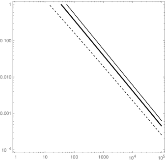
Figure 4.1. Log-log contour plot of the non-oscillatory component $g_{8}\left(r\left(k\right),k\right)$ in (4.1) for different values of $\epsilon$ and $1\leq k\leq 10^{5}$, where thin line corresponds to $\epsilon=10^{-16}$, thick line to $\epsilon=10^{-9}$ and dashed line to $10^{-2}$.

Next we consider the difference between the real part of $G$ in (1.1) and $g_{n}$,

(4.5) $$q_{n}\left(r,k\right)=\mathcal{R}e\left(g_{n,oscill}\right)\left(r,k\right)=\frac{1}{4\pi}\frac{\cos kr}{r}-g_{n}\left(r,k\right),$$

and examine its behavior at $r=0$.

Lemma 4.

The difference

(4.6) $$\mathcal{R}e\left(g_{n,oscill}\right)\left(\mathbf{r},k\right)=\frac{1}{4\pi}\frac{\cos k\left\|\mathbf{r}\right\|}{\left\|\mathbf{r}\right\|}-g_{n}\left(\left\|\mathbf{r}\right\|,k\right),$$

has continuous partial derivatives at zero up to order $2n-2$. The Taylor expansion of $q_{n}$ at $r=\left\|\mathbf{r}\right\|=0$ yields

$$q_{1}\left(r,k\right) = \frac{k}{4\pi}\left(1-kr+\mathcal{O}\left(\left(kr\right)^{2}\right)\right)$$

$$q_{2}\left(r,k\right) = \frac{k}{4\pi}\left(-\frac{\left(kr\right)^{2}}{3}+\frac{\left(kr\right)^{3}}{6}+\mathcal{O}\left(\left(kr\right)^{4}\right)\right)$$

$$q_{3}\left(r,k\right) = \frac{k}{4\pi}\left(-\frac{1}{2}-\frac{\left(kr\right)^{2}}{12}+\frac{7\left(kr\right)^{4}}{240}-\frac{\left(kr\right)^{5}}{90}+\mathcal{O}\left(\left(kr\right)^{6}\right)\right)$$

(4.7) $$q_{4}\left(r,k\right) = \frac{k}{4\pi}\left(-1+\frac{\left(kr\right)^{4}}{120}-\frac{\left(kr\right)^{6}}{840}+\frac{\left(kr\right)^{7}}{2520}+\mathcal{O}\left(\left(kr\right)^{8}\right)\right)$$

$$q_{5}\left(r,k\right) = \frac{k}{4\pi}\left(\right.-\frac{13}{8}+\frac{\left(kr\right)^{2}}{16}+\frac{\left(kr\right)^{4}}{320}-\frac{\left(kr\right)^{6}}{40320}+$$

$$\frac{83\left(kr\right)^{8}}{2903040}-\frac{\left(kr\right)^{9}}{113400}+\mathcal{O}\left(\left(kr\right)^{10}\right)\left.\right)$$

$$\dots$$ .

Proof.

The function $q_{n}$ in (4.5) is the inverse Fourier transform of rotationally invariant function (3.4),

(4.8) $$\mathcal{R}e\left(g_{n,oscill}\right)\left(r,k\right)=\frac{1}{2\pi^{2}r}\mbox{p.v.}\int_{0}^{\infty}\frac{p}{p^{2}-k^{2}}\frac{\left(2k^{2}\right)^{n}}{\left(p^{2}+k^{2}\right)^{n}}\sin\left(pr\right)dp.$$

Formally $\mathcal{R}e\left(g_{n,oscill}\right)$ in (4.8) is an even function of $r$ and, as long as the necessary derivatives exist, only even powers can appear in its Taylor expansion. Taking $2n-2$ derivatives of $g_{n,oscill}\left(r,k\right)$ with respect to $r$ correspond to multiplying the integrand in (4.8) by powers $p^{j}$, $0<j\leq 2n-2$ which changes the rate of decay of the integrand from $\mathcal{O}\left(p^{-2n-1}\right)$ to as low as $\mathcal{O}\left(p^{3}\right)$ so that the integrals for these derivatives exist. Replacing $r$ by $\left\|\mathbf{r}\right\|$, we observe that continuous partial derivatives at zero exist up to the order $2n-2$. As we see in (4.7), the next term in the expansion does not yield a continuous derivative of (4.6) at zero. Several examples of expansions of (4.5) using (4.1) are presented in (4.7) . ∎

In Figure 4.2 we plot $g_{4,oscill}$ to illustrate the behavior of this oscillatory component.

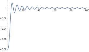
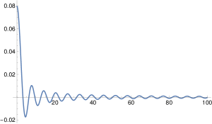
(a)                                                                                       (b)

Figure 4.2. The real part $\mathcal{R}e\left(g_{4,oscill}\right)\left(r,k\right)=\frac{1}{4\pi}\cos\left(kr\right)/r-g_{4}\left(r,k\right)$ (4.5) (a) and the imaginary part $\frac{1}{4\pi}\sin\left(kr\right)/r$ of the oscillatory component (b) for $k=1$.

5. Spatial representations in $\mathbb{R}^{2}$

To avoid confusion, we denote the inverse Fourier transform of (3.5) in dimension $d=2$ as $h_{n}\left(r\right)$. We have

Lemma 5.

The inverse Fourier transform of (3.5) in dimension $d=2$ yields

(5.1) $$h_{n}\left(r,k\right)=\frac{1}{2\pi}\sum_{j=0}^{n-1}\frac{\left(kr\right)^{j}}{j!}K_{j}\left(kr\right),$$

where $K$ is the modified Bessel function of the second kind.

Proof.

Using (3.5), we obtain

(5.2) $$h_{n}\left(r,k\right) = \frac{1}{\left(2\pi\right)^{2}}\int_{\mathbb{R}^{2}}\widehat{g}_{n}\left(\left\|\mathbf{p}\right\|\right)e^{i\mathbf{p}\cdot\mathbf{r}}d\mathbf{p}$$

$$= \frac{1}{2\pi}\sum_{j=0}^{n-1}\int_{0}^{\infty}\frac{\left(2k^{2}\right)^{j}}{\left(p^{2}+k^{2}\right)^{j+1}}J_{0}\left(pr\right)pdp$$

The integral in (5.2) is available in [11, Formula 6.565.4] leading to (5.1).

Next we consider the difference between the real part of $G$ in (1.1) and $h_{n}$ in dimension $d=2$,

(5.3) $$v_{n}\left(r,k\right)=\mathcal{R}e\left(h_{n,oscill}\right)\left(r,k\right)=-\frac{1}{4}Y_{0}\left(kr\right)-h_{n}\left(r,k\right),$$

and examine its behavior at $r=0$. ∎

Lemma 6.

The difference

(5.4) $$\mathcal{R}e\left(h_{n,oscill}\right)\left(\mathbf{r},k\right)=-\frac{1}{4}Y_{0}\left(k\left\|\mathbf{r}\right\|\right)-h_{n}\left(\left\|\mathbf{r}\right\|,k\right)$$

has continuous partial derivatives at $\left\|\mathbf{r}\right\|=0$ up to order $2n$. The Taylor expansion of $v_{n}\left(r,k\right)$ yields

$$v_{1}\left(r,k\right) = \frac{-1+\gamma-\log 2}{4\pi}\left(kr\right)^{2}+\mathcal{O}\left(\left(kr\right)^{2}\log\left(kr\right)\right)$$

$$v_{2}\left(r,k\right) = -\frac{1}{2\pi}-\frac{1}{8\pi}\left(kr\right)^{2}+\frac{5-4\gamma+4\log 2}{128\pi}\left(kr\right)^{4}+\mathcal{O}\left(\left(kr\right)^{4}\log\left(kr\right)\right)$$

$$v_{3}\left(r,k\right) = -\frac{1}{\pi}+\frac{1}{64\pi}\left(kr\right)^{4}+\frac{-4+3\gamma-3\log 2}{1728\pi}\left(kr\right)^{6}+\mathcal{O}\left(\left(kr\right)^{6}\log\left(kr\right)\right)$$

$$v_{4}\left(r,k\right) = -\frac{5}{3\pi}+\frac{1}{12\pi}\left(kr\right)^{2}+\frac{1}{192\pi}\left(kr\right)^{4}-\frac{5}{6912\pi}\left(kr\right)^{6}$$

$$+ \frac{11-8\gamma+8\log 2}{147456\pi}\left(kr\right)^{8}+\mathcal{O}\left(\left(kr\right)^{8}\log\left(kr\right)\right)$$

$$v_{5}\left(r,k\right) = -\frac{8}{3\pi}+\frac{1}{6\pi}\left(kr\right)^{2}-\frac{1}{3456\pi}\left(kr\right)^{6}+\frac{1}{55296\pi}\left(kr\right)^{8}$$

$$+ \frac{-169+120\gamma-120\log 2}{110592000\pi}\left(kr\right)^{10}+\mathcal{O}\left(\left(kr\right)^{10}\log\left(kr\right)\right)$$

$$\dots$$ ,

where $\gamma$ is Euler’s constant.

Proof.

The function $v_{n}$ in (5.3) is the inverse Fourier transform of rotationally invariant function (3.4) in dimension $d=2$,

$$\mathcal{R}e\left(h_{n,oscill}\right)\left(r,k\right)=\frac{1}{2\pi}\int_{0}^{\infty}\frac{p}{p^{2}-k^{2}}\frac{\left(2k^{2}\right)^{n}}{\left(p^{2}+k^{2}\right)^{n}}J_{0}\left(pr\right)pdp.$$

We use the same argument to count the number of continuous derivatives of $h_{n,oscill}\left(\mathbf{r},k\right)$ as in Lemma 4. Several examples of expansions of (5.3) using (5.1) are presented in (6) . ∎

6. Integral representations

Integral representations via Gaussians of kernels of non-oscillatory operators have been used as a starting point to obtain their accurate multiresolution approximations via a linear combination of Gaussians, see e.g. [16, 7, 3, 8, 9, 4, 15, 1]. For any $\epsilon>0$, kernels are approximated with accuracy $\epsilon$ by a linear combination of Gaussians where the number of terms is shown to be $\mathcal{O}\left(\left(\log\epsilon^{-1}\right)^{2}+\log\delta^{-1}\right)$, where $\delta$ defines the interval of validity of the approximation, e.g. $\delta<r<\delta^{-1}$ (see e.g. [9]). This estimate is somewhat conservative since the actual number of terms appears to be $\mathcal{O}\left(\log\epsilon^{-1}+\log\delta^{-1}\right)$. In what follows we construct integral representations via Gaussians of the non-oscillatory components of the Green’s function (1.1).

Lemma 7.

The function $g_{n}\left(r,k\right)$ in dimension $d=3$ has an integral representation

(6.1) $$g_{n}\left(r,k\right)=\int_{-\infty}^{\infty}e^{-r^{2}e^{t}/4}w_{n}\left(k,t\right)dt$$

where

$$w_{n}\left(k,t\right)=\frac{1}{8\pi^{3/2}}e^{-k^{2}e^{-t}+\frac{1}{2}t}\left(\sum_{j=0}^{n-1}\frac{\left(2k^{2}e^{-t}\right)^{j}}{j!}\right).$$

Proof.

Using the integral (see e.g. [9, eq. 2])

$$\rho^{-j-1}=\frac{1}{j!}\int_{-\infty}^{\infty}e^{-\rho e^{t}+\left(j+1\right)t}dt,$$

we obtain from (4.3) and (3.5)

(6.2) $$g_{n}\left(r,k\right) = \frac{1}{\left(2\pi\right)^{3}}\sum_{j=0}^{n-1}\int_{\mathbb{R}^{3}}\frac{\left(2k^{2}\right)^{j}}{\left(\left\|\mathbf{p}\right\|^{2}+k^{2}\right)^{j+1}}e^{i\mathbf{p}\cdot\mathbf{r}}d\mathbf{p}$$

$$\frac{1}{\left(2\pi\right)^{3}}\int_{\mathbb{R}^{3}}\left(\sum_{j=0}^{n-1}\frac{\left(2k^{2}\right)^{j}}{j!}\int_{-\infty}^{\infty}e^{-\left(k^{2}+\left\|\mathbf{p}\right\|^{2}\right)e^{t}+\left(j+1\right)t}dt\right)e^{i\mathbf{p}\cdot\mathbf{r}}d\mathbf{p}$$

$$= \frac{1}{\left(2\pi\right)^{3}}\int_{\mathbb{R}^{3}}\left(\int_{-\infty}^{\infty}e^{-e^{t}\left\|\mathbf{p}\right\|^{2}}\left(\sum_{j=0}^{n-1}\frac{\left(2k^{2}e^{t}\right)^{j}}{j!}\right)e^{-k^{2}e^{t}+t}dt\right)e^{i\mathbf{p}\cdot\mathbf{r}}d\mathbf{p}$$

$$= \int_{-\infty}^{\infty}\left(\frac{1}{\left(2\pi\right)^{3}}\int_{\mathbb{R}^{3}}e^{-e^{-t}\left\|\mathbf{p}\right\|^{2}}e^{i\mathbf{p}\cdot\mathbf{r}}d\mathbf{p}\right)\sum_{j=0}^{n-1}\frac{\left(2k^{2}e^{-t}\right)^{j}}{j!}e^{-k^{2}e^{-t}-t}dt,$$

where in the last integral we changed the order of integration and replaced $t$ by $-t$ for convenience. Computing the inverse Fourier transform of rotationally invariant function $e^{-e^{-t}\left\|\mathbf{p}\right\|^{2}}$ in dimension $d=3$, we have

$$\frac{1}{\left(2\pi\right)^{3}}\int_{\mathbb{R}^{3}}e^{-e^{-t}\left\|\mathbf{p}\right\|^{2}}e^{i\mathbf{r}\cdot\mathbf{p}}d\mathbf{p} = \frac{1}{2\pi^{2}r}\int_{0}^{\infty}e^{-e^{-t}p^{2}}\sin\left(pr\right)pdp$$

$$= \frac{1}{8\pi^{3/2}}e^{-r^{2}e^{t}/4}e^{\frac{3}{2}t}.$$

Substituting (6) into (6.2), we arrive at (6.1). ∎

Turning to dimension $d=2$, we have

Lemma 8.

The function $h_{n}$ in dimension $d=2$ has an integral representation

(6.4) $$h_{n}\left(r,k\right)=\int_{-\infty}^{\infty}e^{-r^{2}e^{t}/4}\omega_{n}\left(k,t\right)dt,$$

where

$$\omega_{n}\left(k,t\right)=\frac{1}{4\pi}e^{-k^{2}e^{-t}}\left(\sum_{j=0}^{n-1}\frac{\left(2k^{2}e^{-t}\right)^{j}}{j!}\right).$$

Proof.

Using integral representation of functions $K_{j}$ derived in [9, eq. 36], we have

$$\left(kr\right)^{j}K_{j}\left(kr\right)=2^{j-1}k^{2j}\int_{0}^{\infty}e^{-r^{2}s/4-k^{2}/s}s^{-j-1}ds,$$

and, therefore,

$$\frac{1}{2\pi}\sum_{j=0}^{n-1}\frac{\left(kr\right)^{j}}{j!}K_{j}\left(kr\right)=\frac{1}{4\pi}\int_{0}^{\infty}e^{-r^{2}s/4-k^{2}/s}\sum_{j=0}^{n-1}\frac{\left(2k^{2}\right)^{j}}{j!}s^{-j-1}ds.$$

Changing variables $s=e^{t}$, we obtain (6.4). ∎

7. Discretization of integral representations

Spatial integral representations of non-oscillatory components in (6.1) and (6.4) lead to approximations of functions $g_{n}$ and $h_{n}$ by a linear combination of Gaussians. In both cases, for $r>\delta$, the integrands decay super exponentially for $t\to\pm\infty$, where the rate of decay for $t\to-\infty$ is controlled by $k$. Heuristically, by selecting a finite interval of integration so that the integrands and their derivatives are negligible outside that interval, any user selected accuracy $\epsilon$ can be achieved using the trapezoidal rule. The resulting sum is a linear combination of Gaussians which may be viewed as a multiresolution approximation of the non-oscillatory component.

As a result, we obtain a separated multiresolution approximation of the kernel of the non-oscillatory component of the Helmholtz operator. There are several approaches to apply this kernel rapidly in $\mathcal{O}\left(k^{d}\left(\log\epsilon^{-1}\right)^{2}\right)$ operations, for example via algorithms in [2] or via the Fast Gauss transform in [13, 14]. We refer to [6, 5] for the details of algorithms for applying both the oscillatory and the non-oscillatory (singular) components.

As an example, we describe an approximation of $g_{4}\left(r,k\right)$ where $k=100$. We discretize the integral in (6.1) as

(7.1) $$\widetilde{g}_{4}\left(r,k\right)=\Delta\sum_{m=20}^{200}e^{-r^{2}e^{m\Delta}/4}w_{4}\left(k,m\Delta\right),\,\,\,\Delta=\frac{1}{4},\,\,\,k=100,\,\,\,r=\left\|\mathbf{r}\right\|.$$

Near the singularity of $g_{4}\left(r,k\right)$, on the interval $10^{-10}\leq r\leq 10^{-3}$, we use the relative error

(7.2) $$e_{0}\left(r\right)=\log_{10}\left|\frac{g_{4}\left(r,k\right)-\widetilde{g}_{4}\left(r,k\right)}{g_{4}\left(r,k\right)}\right|,$$

and on the interval $10^{-3}\leq r\leq 40/k+2\log_{10}k/k$ (or $10^{-3}\leq r\leq 44/100$, see Remark 3) the absolute error,

(7.3) $$e_{1}\left(r\right)=\log_{10}\left|g_{4}\left(r,k\right)-\widetilde{g}_{4}\left(r,k\right)\right|.$$

These approximation errors are illustrated in Figure 7.1. The terms of the linear combination of Gaussians in (7.1) can be applied to a function in parallel. Also we note that the Gaussians with large exponents can be treated as approximations to a delta function and such terms can be combined reducing the overall number of terms.

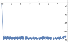
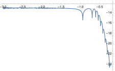
Figure 7.1. The relative error $e_{0}\left(10^{x}\right)$ in (7.2) for $-10\leq x\leq 3$ and the absolute error $e_{1}\left(10^{x}\right)$ in (7.3) for $-3\leq x\leq\log_{10}\left(0.44\right)$.

8. Conclusions

The Helmholtz operator appears in many problems of mathematical physics and is also part of more complicated Green’s functions. In particular, the components of the Dyadic Green’s function in electromagnetics are derivatives of the the Helmholtz Green’s function. Therefore, the splitting into the oscillatory and the non-oscillatory components can be obtained for the Dyadic Green’s function as well. We expect several problems beyond the one described in this paper to be addressed using our results.

9. Acknowledgments

The author would like to thank Brad Alpert (NIST) and Lucas Monzón (CU) for suggestions to improve the manuscript.

References

- [1] J. Anderson, R.J. Harrison, B. Sundahl, W. S. Thornton, and G. Beylkin. Real-space quasi-relativistic quantum chemistry. Computational and Theoretical Chemistry, 1175:112711, 2020.
- [2] G. Beylkin, V. Cheruvu, and F. Pérez. Fast adaptive algorithms in the non-standard form for multidimensional problems. Appl. Comput. Harmon. Anal., 24(3):354–377, 2008.
- [3] G. Beylkin, R. Cramer, G.I. Fann, and R.J. Harrison. Multiresolution separated representations of singular and weakly singular operators. Appl. Comput. Harmon. Anal., 23(2):235–253, 2007.
- [4] G. Beylkin, G. Fann, R. J. Harrison, C. Kurcz, and L. Monzón. Multiresolution representation of operators with boundary conditions on simple domains. Appl. Comput. Harmon. Anal., 33:109–139, 2012. http://dx.doi.org/10.1016/j.acha.2011.10.001.
- [5] G. Beylkin, C. Kurcz, and L. Monzón. Fast algorithms for Helmholtz Green’s functions. Proc. R. Soc. A, 464(2100):3301–3326, 2008. doi:10.1098/rspa.2008.0161.
- [6] G. Beylkin, C. Kurcz, and L. Monzón. Fast convolution with the free space Helmholtz Green’s function. J. Comp. Phys., 228(8):2770–2791, 2009.
- [7] G. Beylkin and M. J. Mohlenkamp. Algorithms for numerical analysis in high dimensions. SIAM J. Sci. Comput., 26(6):2133–2159, July 2005.
- [8] G. Beylkin, M. J. Mohlenkamp, and F. Pérez. Approximating a wavefunction as an unconstrained sum of Slater determinants. Journal of Mathematical Physics, 49(3):032107, 2008.
- [9] G. Beylkin and L. Monzón. Approximation of functions by exponential sums revisited. Appl. Comput. Harmon. Anal., 28(2):131–149, 2010.
- [10] I. M. Gel’fand and G. E. Shilov. Generalized functions. Vol. 1. Academic Press, New York, 1964. Properties and operations, Translated from the Russian by Eugene Saletan.
- [11] I. S. Gradshteyn, I. M. Ryzhik, A. Jeffrey, and D. Zwillinger. Table of integrals, series, and products. Academic Press, 7 edition, 2007.
- [12] L. Grafakos. Classical and modern Fourier analysis. Pearson Education, Inc., 2004.
- [13] L. Greengard and J. Strain. The fast Gauss transform. SIAM J. Sci. Stat. Comput., 12(1):79–94, 1991.
- [14] L. Greengard and X. Sun. A new version of the fast Gauss transform. In Proceedings of the international congress of mathematicians, volume III (Extra Vol.), pages 575–584, 1998.
- [15] R. J. Harrison, G. Beylkin, F. A. Bischoff, J. A. Calvin, G. I. Fann, J. Fosso-Tande, D. Galindo, J.R Hammond, R. Hartman-Baker, J.C. Hill, J. Jia, J.S. S. Kottmann, M-J. Y. Ou, L.E. Ratcliff, M.G. Reuter, A.C. Richie-Halford, N.A. Romero, H. Sekino, W.A. Shelton, B.E. Sundahl, W.S. Thornton, E.F. Valeev, A. Vázquez-Mayagoitia, N. Vence, and Y. Yokoi. MADNESS: a multiresolution, adaptive numerical environment for scientific simulation. SIAM J. Sci. Comput., 38(5):S123–S142, 2016. see also arXiv preprint arXiv:1507.01888.
- [16] R.J. Harrison, G.I. Fann, T. Yanai, Z. Gan, and G. Beylkin. Multiresolution quantum chemistry: basic theory and initial applications. J. Chem. Phys., 121(23):11587–11598, 2004.