Enumeration Kernelizations of Polynomial Size for Cuts of Bounded Degree

Abstract

Enumeration kernelization was first proposed by Creignou et al. [TOCS 2017] and was later refined by Golovach et al. [JCSS 2022] into two different variants: fully-polynomial enumeration kernelization and polynomial-delay enumeration kernelization. In this paper, we consider the Degree-$d$-Cut problem from the perspective of (polynomial-delay) enumeration kenrelization. Given an undirected graph $G=(V,E)$, a cut $F=E(A,B)$ is a degree-$d$-cut of $G$ if every $u\in A$ has at most $d$ neighbors in $B$ and every $v\in B$ has at most $d$ neighbors in $A$. Checking the existence of a degree-$d$-cut in a graph is a well-known NP-Complete problem and is well-studied in parameterized complexity [Algorithmica 2021, IWOCA 2021]. This problem also generalizes a well-studied problem Matching Cut (set $d=1$) that has been a central problem in the literature of polynomial-delay enumeration kernelization. In this paper, we study three different enumeration variants of this problem, Enum Deg-$d$-Cut, Enum Min Deg-$d$-Cut and Enum Max Deg-$d$-Cut that intends to enumerate all the degree-$d$-cuts, all the minimal degree-$d$-cuts and all the maximal degree-$d$-cuts respectively. We consider various structural parameters of the input and provide polynomial-delay enumeration kernels for Enum Deg-$d$-Cut and Enum Max Deg-$d$-Cut and fully-polynomial enumeration kernels of polynomial size for Enum Min Deg-$d$-Cut.

1 Introduction

Enumeration is one of the fundamental tasks in theoretical computer science. Given an instance of a combinatorial optimization problem, the enumeration problem asks to output each of the feasible solutions of that instance one by one with no duplicates. In particular, enumerating all the solutions to a given computational problem has applications in various domains, such as web search engines, bioinformatics, and databases. There are many combinatorial optimization problems for which outputting an optimal solution can be achieved in polynomial-time. But, the number of optimal solutions can be exponential in the input size. For such problems, it is desirable that the collection of all the optimal solutions can be outputted without duplicates ((i.e. enumerated) with a polynomial-delay. In other words, the objective is to have algorithms where the time taken between outputting two consecutive solutions is polynomial in the input size. Nonetheless, in the case of NP-hard problems, the likelihood of the existence of a polynomial-time algorithm capable of producing even a single optimal solution is deemed improbable. It is noted that parameterized complexity has been viewed as a possible way around this obstacle by extending the notion of ‘polynomial-time solvability’ to NP-hard decision problems (see Section 2 for definitions and see [12, 31, 16] for more details) by designing algorithms (called fixed-parameter algorithms or FPT algorithms) that run in polynomial-time on inputs with a bounded value of carefully chosen parameters. For NP-hard problems, it is therefore desirable to have algorithms that enumerate the set of all solutions with no duplicates in FPT-delay. What this means is that the time taken between outputting two consecutive solutions satisfying a given property (if any) admits FPT-running time. Enumerating all the feasible solutions satisfying some particular property has been studied in parameterized algorithms in various contexts. For instance, given a graph $G$, if we are to obtain a connected or $p$-(edge)-connected vertex cover of size at most $k$, the first step is to enumerate all the minimal vertex covers of size at most $k$ (see [29, 18]). Similar ideas are used to compute a $p$-edge-connected hitting sets in graphs as well [17]. Several other enumeration algorithms in the literature [22] are built on the notion of bounded search trees.

Kernelization or parameterized preprocessing is one of the most important steps to obtain efficient parameterized algorithms (see [20]). The quality of a kernelization algorithm is usually determined by the size of the output instance. The running time is always required to be polynomial in the input size. Some parameterized problems are also well-studied in the setting of enumeration kernelization. Damaschke [13] introduced a terminology called full kernel from the perspective of parameterized enumeration problems. A full kernel means that there is a polynomial-time preprocessing algorithm that outputs a smaller instance of the same problem, which contains a compact representation of all the solutions of size at most $k$. This definition was found to be too restrictive as they were limited to only minimization problems. In order to overcome this issue, Creignou et al [10, 11, 9] introduced a modified notion of enumeration kernel. Informally, it consisted of a preprocessing algorithm and a solution-lifting algorithm. The preprocessing algorithm outputs an instance of size bounded by a function of the parameter. Given a solution to the output instance, the solution-lifting algorithm outputs a collection of solutions to the original instance satisfying some properties.

But, Golovach et al. [21] observed that this definition is also weak as the solution-lifting algorithm can have FPT-delay running time. In fact that the existence of any FPT-delay enumeration algorithm will automatically imply an enumeration kernelization of constant size as per Creignou et al. [11]. To overcome this limitation, Golovach et al. [21] have introduced a refined notion of parameterized enumeration kernel called polynomial-delay enumeration kernelization (see Section 2 for formal definitions). In their paper, Golovach et al. [21] have studied the problem that intends to “enumerate all (maximal/minimal) matching cuts” with respect to several structural parameters. The decision version of Matching Cut is a well-studied problem (see [1, 2, 26, 7, 28, 24]). The classical version of this problem was first proved to be NP-Complete by Chvatal [8]. A natural generalization of matching cut, called degree-$d$-cut was introduced by Gomes and Sau [14] in which they have studied the parameterized and kernelization complexity of finding a degree-$d$-cut in graphs with respect to several structural parameters, e.g., cluster vertex deletion set, treewidth etc. Given a graph $G=(V,E)$, a cut is a bipartition of its vertex set $V(G)$ into two nonempty sets $A$ and $B$, denoted by $(A,B)$. The set of all edges with one endpoint in $A$ and the other in $B$ is called the edge cut or the set of crossing edges of $(A,B)$. The edge cut of $(A,B)$ is usually denoted by $F=E_{G}(A,B)$. A cut $(A,B)$ of $G$ is said to be a degree-$d$-cut if every vertex of $A$ has at most $d$ neighbors in $B$ and every vertex of $B$ has at most $d$ neighbors in $A$. Equivalently an edge cut $F$ is a degree-$d$-cut if the subgraph $G(V,F)$ of $G$ is a graph of degree at most $d$. Observe that if $d=1$, this is the same as matching cut. Note that not every graph admits a degree-$d$-cut. For a fixed integer $d\geq 1$, the Degree-$d$-Cut is defined as follows.

Degree-$d$-Cut Input: An undirected graph $G=(V,E)$. Question: Is there a cut $(A,B)$ of $G$ such that every vertex $u\in A$ has at most $d$ neighbors in $B$ and every vertex $u\in B$ has at most $d$ neighbors in $A$?

Gomes and Sau [14] proved that for every fixed integer $d\geq 1$, Degree-$d$-Cut is NP-hard even in $(2d+2)$-regular graphs and studied this problem from parameterized and kernelization complexity perspective. Being motivated by the works on polynomial-delay enumeration kernelization on Matching Cut by Golovach et al. [21] and the works on Degree-$d$-Cut (for every fixed integer $d\geq 1$) by Gomes and Sau [14], we initiate a systematic study on the Degree-$d$-Cut problem from the perspective of polynomial-delay enumeration kernelization. A degree-$d$-cut $F$ is a minimal degree-$d$-cut of $G$ if it is inclusion-wise minimal, i.e. no proper subset of $F$ is a degree-$d$-cut of $G$. Similarly, a degree-$d$-cut of $G$ is maximal if no proper superset of $F$ is a degree-$d$-cut of $G$. In this paper, we focus on the problems involving the enumeration of all minimal degree-$d$-cuts, enumerate all maximal degree-$d$-cuts and enumerate all the degree-$d$-cuts of an input graph. These problems are denoted as Enum Min Deg-$d$-Cut, Enum Max Deg-$d$-Cut, and Enum Deg-$d$-Cut, respectively. The formal definitions are stated as follows.

Enum Deg-$d$-Cut Input: An undirected graph $G=(V,E)$. Goal: Enumerate all the degree-$d$-cuts of $G$.

Enum Min Deg-$d$-Cut Input: An undirected graph $G=(V,E)$. Goal: Enumerate all minimal degree-$d$-cuts of $G$.

Enum Max Deg-$d$-Cut Input: An undirected graph $G=(V,E)$. Goal: Enumerate all maximal degree-$d$-cuts of $G$.

Our Contributions and Motivations Behind the Choice of Parameters: We generalize various previously reported results on Enum Matching Cut and present enumeration kernelizations of polynomial size for Enum Min Deg-$d$-Cut, Enum Deg-$d$-Cut, and Enum Max Deg-$d$-Cut for every fixed integer $d\geq 1$. Since the decision version Degree-$d$-Cut is NP-hard [8], it is unlikely that Enum Deg-$d$-Cut, Enum Min Deg-$d$-Cut, and Enum Max Deg-$d$-Cut can admit algorithms that enumerate the corresponding solutions with polynomial-delay. Moreover, several structural properties of degree-$d$-cuts are more complicated than matching cuts. Therefore, Enum Deg-$d$-Cut, Enum Min Deg-$d$-Cut and Enum Max Deg-$d$-Cut are interesting problems to study. In this paper, we consider the size of minimum vertex cover (vc), the neighborhood diversity (nd), and clique-partition number (pc) of the input graph as the parameters. The motivation behind the choice of these parameters is the following. In the context of a parameterized problem, if it is established that the problem does not allow for a (polynomial-delay) enumeration kernelization of polynomial size concerning a specific parameter, it is logical to opt for a parameter that is either structurally larger or incomparable to the aforementioned parameter. Similarly, if a parameterized problem is acknowledged to permit a (polynomial-delay) enumeration kernelization of polynomial size concerning a particular parameter, it is intuitive/natural to select a parameter that is either structurally smaller or incomparable to the mentioned parameter. Enum Deg-$d$-Cut, Enum Min Deg-$d$-Cut, and Enum Max Deg-$d$-Cut do not admit (polynomial-delay enumeration) kernelizations of polynomial size when parameterized by a combined parameter of solution size, maximum degree, and treewidth of the input graph (see [14]). Note that treewidth is a structurally smaller parameter than treedepth that is structurally smaller than the vertex cover number.

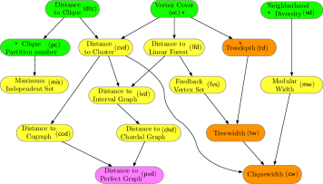
Figure 1: An overview of parameter hierarchy. Some relation between the parameters are ${\textsf{pc}}(G)\leq{\sf dtc}(G)+1$, ${\sf cw}(G)\leq{\sf mw}(G)+2$ and ${\sf cw}(G)\leq{\sf cvd}(G)+3$. For every other arrow from parameter $X$ to parameter $Y$ indicates that $X\leq Y$. A green box says the existence of (polynomial-delay) enumeration kernelizations of polynomial size. An orange box indicates non-existence of enumeration kernelizations of polynomial sized unless ${\sf NP\subseteq coNP/poly}$. A pink box indicates the NP-hardness for constant value of parameter. A yellow box says open status in the existence of (polynomial-delay) enumeration kernelizations of polynomial size. The parameters that are marked as $\star$ have been considered in this paper.

Since the size (vc) of a minimum vertex cover is provably larger than the treedepth of the graph. So, we consider to choose vertex cover as one of the parameters. In addition, we also choose neighborhood diversity (nd) and clique partition number (pc) both of which are incomparable to the vertex cover number. We refer to Figure 1 for an illustration of parameters. Additionally, we refer to Table 1 for a short summary of our results.

Our main results are enumeration kernelizations of polynomial size when the parameter is the size of a minimum vertex cover, i.e. vc of the input graph. We formally prove the following two results in Section 3.

Theorem 1.1.

For every fixed $d\geq 1$, Enum Min Deg-$d$-Cut parameterized by vc admits a fully-polynomial enumeration kernelization containing $\mathcal{O}(d^{3}{\textsf{vc}}^{d+1})$ vertices.

Theorem 1.2.

For every fixed $d\geq 1$, Enum Deg-$d$-Cut and Enum Max Deg-$d$-Cut parameterized by vc admit polynomial-delay enumeration kernelizations with $\mathcal{O}(d^{3}{\textsf{vc}}^{d+1})$ vertices.

Next we consider the neighborhood diversity, i.e. nd of the input graph as the parameter and we prove the following result in Section 4.

Theorem 1.3.

For every fixed $d\geq 1$, Enum Min Deg-$d$-Cut parameterized by nd admit a fully-polynomial enumeration kernelization with $\mathcal{O}(d^{2}{\textsf{nd}})$ vertices. Moreover, Enum Deg-$d$-Cut and Enum Max Deg-$d$-Cut admit polynomial-delay enumeration kernelizations with $\mathcal{O}(d^{2}{\textsf{nd}})$ vertices.

Finally, in Section 5, we consider the size of a clique partition number, i.e. pc as the parameter and prove the following result.

Theorem 1.4.

For every fixed $d\geq 1$, Enum Deg-$d$-Cut, Enum Min Deg-$d$-Cut, and Enum Max Deg-$d$-Cut parameterized by pc admit bijective enumeration kernelizations with $\mathcal{O}({\textsf{pc}}^{d+2})$ vertices.

Parameter $k$	Enum Deg-$d$-Cut	Enum Min Deg-$d$-Cut	Enum Max Deg-$d$-Cut
vertex cover number ($\star\star$)	$\mathcal{O}(d^{3}{k}^{d+1})$-vertex delay enum-kernel (Theorem 1.2)	$\mathcal{O}(d^{3}{k}^{d+1})$-vertex full enum-kernel (Theorem 1.1)	$\mathcal{O}(d^{3}{k}^{d+1})$-vertex delay enum-kernel (Theorem 1.2)
neighborhood diversity ($\star\star$)	$\mathcal{O}(d^{2}k)$-vertex delay enum-kernel (Theorem 1.3)	$\mathcal{O}(d^{2}k)$-vertex full enum-kernel (Theorem 1.3)	$\mathcal{O}(d^{2}k)$-vertex delay enum-kernel (Theorem 1.3)
clique partition number ($\star\star$)	$\mathcal{O}({k}^{{d}+2})$-vertex bijective enum-kernel (Theorem 1.4)	$\mathcal{O}({k}^{{d}+2})$-vertex bi-enum-kernel (Theorem 1.4)	$\mathcal{O}({k}^{d+2})$-vertex bijective enum-kernel (Theorem 1.4)
distance to clique	$\mathcal{O}({k}^{{d}+2})$-vertex bijective enum-kernel	$\mathcal{O}({k}^{{d}+2})$-vertex bi-enum-kernel	$\mathcal{O}({k}^{d+2})$-vertex bijective enum-kernel
treedepth, treewidth, and cliquewidth	No polynomial size delay enum-kernel ($\star$) (Proposition 2.2)	No polynomial size delay enum-kernel ($\star$) (Proposition 2.2)	No polynomial size delay enum-kernel ($\star$) (Proposition 2.2)

Table 1: Summary of our results. Here, “delay enum-kernel” means polynomial-delay enumeration kernelization, “full enum-kernel” means fully-polynomial enumeration kernelization, and “bi-enum-kernel” means bijective enumeration kernelization. A ($\star$) means the lower bound assumes ${\rm NP\not\subseteq coNP/poly}$. The results marked as ($\star\star$) are the results proved in this paper.

Related Work: Xiao and Nagamochi [35] had studied a different variant of Degree-$d$-Cut from the perspective of parameterized complexity. We refer to a survey by Wasa [34] for a detailed overview of enumeration algorithms. Bentert et al. [3] have introduced a notion of advice enumeration kernels where they provide an extension to the enumeration problem by Creignou et al. [11] where a small amount of advice is needed rather than the whole input. Enumeration of solutions with some lexicographic order is also studied (see [4, 23]). Counting problems are closely related to enumeration problems. A concrete survey by Thilikos [33] is also available for compact representation of parameterized counting problems. Later, several other studies have also happened in parameterized counting problems, including a few in temporal graph models also (see [30, 19, 6]). Very recently, Lokshtanov et al.[27] have formally introduced the framework of kernelization for counting problems.

2 Preliminaries

Sets, Numbers, and Graph Theory: We use $[r]$ to denote $\{1,\ldots,r\}$ for some $r\in{\mathbb{N}}$ and $A\uplus B$ to denote the disjoint union of the sets $A$ and $B$. For a set $A$, we use $2^{A}$ to denote the power set of $A$. For a finite set $A$ and a nonnegative integer $d\geq 0$, we use ${{A}\choose{d}},{{A}\choose{\leq d}}$, and ${{A}\choose{\geq d}}$ to denote the collection of all subsets of $A$ of size equal to $d$, at most $d$, and at least $d$ respectively. We use standard graph theoretic notations from the book of Diestel [15]. Throughout this paper, we consider undirected graphs. For a subset $X\subseteq V(G)$, $G[X]$ denotes the subgraph induced by the vertex subset $X$. Similarly, $G-X$ denotes the graph obtained after deleting the vertex set $X$; i.e. $G-X=G[V(G)\setminus X]$; for a vertex $u$, we use $G-u$ to represent $G-\{u\}$ for the simplicity. Similarly, for a set of edges $F\subseteq E(G)$ (respectively for $e\in E(G)$), we write $G-F$ (respectively $G-e$) to denote the graph obtained after deleting the edges of $F$ (respectively after deleting $e$) from $G$. Equivalently, for an edge $F\subseteq E(G)$, we use $G-F$ to denote the subgraph $G(V,E\setminus F)$ For a vertex $v$, we denote by $N_{G}(v)$ the open neighborhood of $v$, i.e. the set of vertices that are adjacent to $v$ and by $N_{G}[v]$ the closed neighborhood of $v$. Formally, $N_{G}[v]=N_{G}(v)\cup\{v\}$. We omit these subscripts when the graph $G$ is clear from the context. Given a graph $G=(V,E)$, a set $M\subseteq V(G)$ is said to be a module of $G$ if every pair of vertices of $M$ has the same neighborhood outside $M$. Formally, for every $u,v\in M$, $N_{G}(u)\setminus M=N_{G}(v)\setminus M$. A modular decomposition of $G$ is a decomposition of the vertices of $G$ into vertex-disjoint modules. Formally, ${\mathcal{U}}=\{X_{1},\ldots,X_{k}\}$ is a modular decomposition of $G$ if $\cup_{i=1}^{k}X_{i}=V(G)$ and $X_{i}\cap X_{j}=\emptyset$ for every $i\neq j$. A set of vertices $S\subseteq V(G)$ is called vertex cover if for every $uv\in E(G)$, $u\in S$ or $v\in S$ (or both). The following observation [14] is a fundamental structural property of degree-$d$-cuts that we use throughout our paper.

Observation 2.1.

Let $G$ be a graph that contains a clique $C$ containing at least $2d+1$ vertices. Then, for any degree-$d$-cut $(A,B)$ of $G$, either $C\subseteq A$ or $C\subseteq B$.

We introduce a graph operation that we were unable to find in the literature. Let $G$ be an undirected graph such that $u\in V(G)$. We define a graph operation attach a pendant clique $C$ of $r$ vertices into $u$ when a clique $C$ containing $r$ vertices is attached to $G$ such that $C\cap V(G)=\{u\}$. In short form, we often call this graph operation attach an $r$-vertex pendant clique into $u$.

Parameterized Complexity and Kernelization: A parameterized problem is denoted by $L\subseteq\Sigma^{*}\times{\mathbb{N}}$ where $\Sigma$ is a finite alphabet. An instance of a parameterized problem is denoted $(x,k)\in\Sigma^{*}\times{\mathbb{N}}$ where and $k$ is considered as the parameter. A parameterized problem $L$ is said to be fixed-parameter tractable if there is an algorithm ${\mathcal{A}}$ that takes an input instance $(x,k)\in\Sigma^{*}\times{\mathbb{N}}$, runs in $f(k)|x|^{\mathcal{O}(1)}$-time and correctly decides if $(x,k)\in L$ for a computable function $f:{\mathbb{N}}\rightarrow{\mathbb{N}}$. The algorithm ${\mathcal{A}}$ is called fixed-parameter algorithm (or FPT algorithm). An important step to design parameterized algorithms is kernelization (or parameterized preprocessing). Formally, a parameterizezd problem $L\subseteq\Sigma^{*}\times{\mathbb{N}}$ is said to admit a kernelization if there is a polynomial-time procedure that takes $(x,k)\in\Sigma^{*}\times{\mathbb{N}}$ and outputs an instance $(x^{\prime},k^{\prime})$ such that (i) $(x,k)\in L$ if and only if $(x^{\prime},k^{\prime})\in L$, and (ii) $|x^{\prime}|+k^{\prime}\leq g(k)$ for some computable function $g:{\mathbb{N}}\rightarrow{\mathbb{N}}$. It is well-known that a decidable parameterized problem is FPT if and only if it admits a kernelization [12].

Parameterized Enumeration and Enumeration Kernelization: We use the framework for parameterized enumeration was proposed by Creignou et al. [11]. An enumeration problem over a finite alphabet $\Sigma$ is a tuple $(L,{\sf Sol})$ such that

1. $L$ is a decidable problem, and

2. ${\sf Sol}:\Sigma^{*}\rightarrow 2^{\Sigma^{*}}$ is a computable function such that ${\sf Sol}(x)$ is a nonempty finite set if and only if $x\in L$.

Here $x\in\Sigma^{*}$ is an instance, and ${\sf Sol}(x)$ is the set of solutions to instance $x$. A parameterized enumeration problem is defined as a triple $\Pi=(L,\sf Sol,\kappa)$ such that $(L,{\sf Sol})$ satisfy the same as defined in item (i) and (ii) above. In addition to that $\kappa:\Sigma^{*}\rightarrow{\mathbb{N}}$ is the parameter. We define here the parameter as a function $\kappa(x)$ to the input instance, but it is natural to assume that the parameter is given with the input or $\kappa(x)$ can be computed in polynomial-time. An enumeration algorithm ${\mathcal{A}}$ for a parameterized enumeration problem $\Pi$ is a deterministic algorithm that given $x\in\Sigma^{*}$, outputs ${\sf Sol}(x)$ exactly without duplicates and terminates after a finite number of steps. If ${\mathcal{A}}$ outputs exactly ${\sf Sol}(x)$ without duplicates and eventually terminates in $f(\kappa(x))|x|^{\mathcal{O}(1)}$-time, then ${\mathcal{A}}$ is called an FPT-enumeration algorithm. For $x\in L$ and $1\leq i\leq|{\sf Sol}(x)|$, the $i$-th delay of ${\mathcal{A}}$ is the time taken between outputting the $i$-th and $(i+1)$-th solution of ${\sf Sol}(x)$. The $0$-th delay is the precalculation time that is the time from the start of the algorithm until the first output. The $|{\sf Sol}(x)|$-th delay is the postcalculation time that is the time from the last output to the termination of ${\mathcal{A}}$. If the enumeration algorithm ${\mathcal{A}}$ on input $x\in\Sigma^{*}$, outputs ${\sf Sol}(x)$ exactly without duplicates such that every delay is $f(\kappa(x))|x|^{\mathcal{O}(1)}$, then ${{\mathcal{A}}}$ is called an FPT-delay enumeration algorithm.

Definition 2.1.

Let $\Pi=(L,\sf Sol,\kappa)$ be a parameterized enumeration problem. A fully-polynomial enumeration kernelization for $\Pi$ is a pair of algorithms ${\mathcal{A}}$ and ${\mathcal{A}}^{\prime}$ with the following properties.

1. For every instance $x$ of $\Pi$, the kernelization algorithm ${\mathcal{A}}$ computes in time polynomial in $|x|+\kappa(x)$ an instance $y$ of $\Pi$ such that $|y|+\kappa(y)\leq f(\kappa(x))$ for a computable function $f(\cdot)$.

2. For every $s\in{\sf Sol}(y)$, the solution-lifting algorithm ${\mathcal{A}}^{\prime}$ computes in time polynomial in $|x|+|y|+\kappa(x)+\kappa(y)$ a nonempty set of solutions $S_{s}\subseteq{\sf Sol}(x)$ such that $\{S_{s}\mid s\in{\sf Sol}(y)\}$ is a partition of ${\sf Sol}(x)$.

Definition 2.2.

Let $\Pi=(L,{\sf Sol},\kappa)$ be a parameterized enumeration problem. A polynomial-delay enumeration kernelization for $\Pi$ is a pair of algorithms ${\mathcal{A}}$ and ${\mathcal{A}}^{\prime}$ with the following properties.

1. For every instance $x$ of $\Pi$, the kernelization algorithm ${\mathcal{A}}$ computes in time polynomial in $|x|+\kappa(x)$ an instance $y$ of $\Pi$ such that $|y|+\kappa(y)\leq f(\kappa(x))$ for a computable function $f(\cdot)$.

2. For every $s\in{\sf Sol}(y)$, the solution-lifting algorithm ${\mathcal{A}}^{\prime}$ computes with delay in polynomial in $|x|+|y|+\kappa(x)+\kappa(y)$ a nonempty set of solutions $S_{s}\subseteq{\sf Sol}(x)$ such that $\{S_{s}\mid s\in{\sf Sol}(y)\}$ is a partition of ${\sf Sol}(x)$.

Observe that the sizes of the outputs in Definition 2.1 and Definition 2.2, $|y|+\kappa(y)$ is upper bounded by $f(\kappa(x))$ for some computable function $f:{\mathbb{N}}\rightarrow{\mathbb{N}}$. The size of the kernelization is $f(\kappa(x))$. If $f(\cdot)$ is a polynomial function, then the fully-polynomial enumeration kernelization or the polynomial-delay enumeration kernelization for $\Pi$ is of polynomial size. In addition, the Property (ii) of Definition 2.1 and Property (ii) of Definition 2.2 clearly imply that ${\sf Sol}(x)\neq\emptyset$ if and only if ${\sf Sol}(y)\neq\emptyset$. In particular, this second properties for both the above definitions also imply that there is a surjective mapping from ${\sf Sol}(x)$ to ${\sf Sol}(y)$. An enumeration kernelization is bijective if for every $s\in{\sf Sol}(y)$, the solution lifting algorithm produces a unique solution to $\hat{s}\in{\sf Sol}(x)$. It implies that there is a bijection between ${\sf Sol}(y)$ and ${\sf Sol}(x)$. Such kernelization algorithms are also called bijective enumeration kernelizations. It is not very hard to observe that every bijective enumeration kernelization is a fully-polynomial enumeration kernelization and every fully-polynomial enumeration kernelization is a polynomial-delay enumeration kernelization [21]. Golovach et al. [21] have proved the following proposition.

Proposition 2.1.

Let $L$ be a parameterized enumeration problem, the decision version of which is a decidable problem. Then, $L$ admits an FPT-enumeration algorithm if and only if $L$ admits a fully-polynomial enumeration kernelization. Moreover, $L$ admits an FPT-delay enumeration algorithm if and only if $L$ admits polynomial-delay enumeration kernelization. In particular, $L$ can be solved in polynomial-time (or with polynomial-delay) if and only if $L$ admits a fully-polynomial (polynomial-delay) enumeration kernelization of constant size.

Notice that the enumeration kernelizations that can be inferred from the above mentioned proposition does not necessarily have polynomial size. We would like to highlight that the following proposition can be proved by using cross composition framework (see [5]).

Proposition 2.2.

For any fixed $d\geq 1$, Enum Deg-$d$-Cut, Enum Max Deg-$d$-Cut and Enum Min Deg-$d$-Cut do not admit any polynomial-delay enumeration kernelizations of polynomial size when parameterized by the ${\sf td}$ of the input graph unless ${\sf NP\subseteq coNP/poly}$.

3 Enumeration Kernelizations Parameterized by Vertex Cover Number

This section is devoted to the enumeration kernelizations of polynomial size for Enum Deg-$d$-Cut, Enum Min Deg-$d$-Cut, and Enum Max Deg-$d$-Cut when $d$ is a fixed positive integer and the parameter is vc, i.e. the size of a minimum vertex cover of the graph. We can exclude this assumption that an explicit vertex cover is given with the input. We simply invoke a polynomial-time algorithm [32] that outputs a vertex cover $S$ with at most $2{\textsf{vc}}(G)$ vertices. Hence, we consider $(G,S,k)$ as the input instance such that $S$ is a vertex cover of $G$ such that $|S|=k\leq 2{\textsf{vc}}(G)$. The input instance to both the other variants Enum Min Deg-$d$-Cut and Enum Max Deg-$d$-Cut is also the same $(G,S,k)$. The input instance is an undirected graph $G$, and a vertex cover $S$ containing $k$ vertices and let $I=V(G)\setminus S$. Next, we state a lemma that illustrates an important structural property of a degree-$d$-cut $(A,B)$ of the input instance $(G,S,k)$. Given a degree-$d$-cut $(A,B)$ of $G$, the lemma gives a partial characterization of a subset $T\subseteq S$ that can have a nonempty intersection with both $A$ as well as with $B$.

Lemma 3.1.

Let $G$ be an undirected graph, $S$ be a vertex cover of $G$ and $I=V(G)\setminus S$. Moreover, let $T\subseteq S$ such that $|T|\geq 2$ and there are more than $2d$ vertices in $I$ whose neighborhood contains $T$. Then, for any degree-$d$-cut $(A,B)$ of $G$, either $T\subseteq A$ or $T\subseteq B$.

Proof.

For the sake of contradiction, suppose that the premise holds true, but there is a degree-$d$-cut $(A,B)$ of $G$ such that $T\cap A,T\cap B\neq\emptyset$. We consider $v\in I$ such that $T\subseteq N_{G}(v)$. As per the premise, there are at least $2d+1$ vertices in $I$ whose neighborhood contains $T$. Let $\hat{I}_{T}$ be the set of any $2d+1$ vertices from $I$ whose neighborhood contains $T$. That is, for every $v\in\hat{I}_{T}$, $T\subseteq N_{G}(v)$ and $|\hat{I}_{T}|\geq 2d+1$. By pigeon hole principle, at least $d+1$ vertices from $\hat{I}_{T}$ are in $A$ (or in $B$ respectively). Without loss of generality, we assume that $d+1$ vertices from $\hat{I}_{T}$ are in $A$. By our hypothesis, $T\cap A,T\cap B\neq\emptyset$. Then, there is a vertex $x\in T\cap B$ such that $x$ has $d+1$ neighbors in $A$. This leads to a contradiction to the assumption that $(A,B)$ is a degree-$d$-cut of $G$. Similarly, if $d+1$ vertices from $\hat{I}_{T}$ are in $B$, then there is a vertex $x\in T\cap A$ that has $d+1$ neighbors in $B$. This also contradicts the assumption that $(A,B)$ is a degree-$d$-cut of $G$. Hence the claim of the statement holds true. ∎

Note that the statement of the above lemma is a generalization of Observation 1 from [14]. If we put $|T|\geq d+1$ in our statement, then we get Observation 1 from [14]. The above lemma does not explicitly include the case $|T|=1$ but when $|T|=1$, it trivially follows that either $T\subseteq A$ or $T\subseteq B$. Let $I_{d}$ be the vertices of $I$ that has degree at most $d$ in $G$, and $I_{d+1}$ be the vertices of $I$ that has degree at least $d+1$ in $G$.

3.1 Preprocessing Algorithm to Construct the Output Graph

In this section, we describe a marking procedure ${\sf MarkVC}(G,S,k)$, that will be exploited by all the kernelizations in this section.

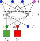
Figure 2: An illustration of attaching pendant cliques for $d=2$ with the set $T=\{x,y\}\subseteq S$. The green, blue, and pink colored vertices are the false twins of $u$ such that $N_{G}(u)=T$. The marked false twins are the red and the blue vertices. The pendant clique $C_{u}$ contains 6 vertices including $u$ and $C_{1}$ contains 7 vertices including $u_{1}$.

Procedure: ${\sf MarkVC}(G,S,k)$:

1. Initialize $H^{*}:=G$ and $S_{0}:=\emptyset$.

2. Mark one arbitrary isolated vertex of $H^{*}$ if exists.

3. For every nonempty set $T\in{{S}\choose{\leq d}}$, let there exists $u\in I_{d}$ such that $N_{G}(u)=T$. If $u$ has at most $2d$ false twins in $I_{d}$, then mark $u$ and all its false twins from $I_{d}$.

4. For every nonempty set $T\in{{S}\choose{\leq d}}$, let there is $u\in I_{d}$ such that $N_{G}(u)=T$. If $u$ has more than $2d$ false twins in $I_{d}$, then mark $u$ and $2d+1$ false twins of $u$ from $I_{d}$. Let $u_{1},\ldots,u_{d-1}\in I_{d}$ be $d-1$ arbitrary marked false twins of $u$. If $u$ has an unmarked false twin, then add a pendant clique $C_{u}$ with $2d+2$ vertices into $u$ and set $S_{0}:=S_{0}\cup(C_{u}\setminus\{u\})$. Then, for every $i\in[d-1]$, add a pendant clique $C_{i}$ with $2d+i+2$ vertices into $u_{i}$ and set $S_{0}:=S_{0}\cup(C_{i}\setminus\{u_{i}\})$. Aee Figure 2 for an illustration with $d=2$ and $|T|=d$.

5. For every nonempty set $T\in{{S}\choose{d+1}}$ mark $\min\{2d+1,|\bigcap\limits_{x\in T}N_{G}(x)\cap I_{d+1}|\}$ arbitrary vertices from $\bigcap\limits_{x\in T}N_{G}(x)\cap I_{d+1}$. Informally, for every $T\in{{S}\choose{d+1}}$, mark $2d+1$ vertices from $I_{d+1}$ that are common neighbors of the vertices of $T$.

We use $Z$ to denote the set of all marked vertices from $I$ and let $H=H^{*}[S\cup Z\cup S_{0}]$. It is straightforward to see that $H$ can be constructed in polynomial-time. The intuition behind adding the pendant cliques (i.e. the vertices of $S_{0}$) is not immediately clear. Towards the end, we will see that the information on the sizes of these pendant cliques will be used in the solution-lifting algorithm to correctly satisfy the Property (ii) of Definition 2.1 and Definition 2.2. The following observation illustrates some important properties of $H$.

Observation 3.1.

The number of vertices in $S_{0}$ is $\mathcal{O}(d^{3}|S|^{d})$ and every connected component of $H[S_{0}]$ is a clique with at least $2d+1$ and at most $3d$ vertices. Moreover, $S\cup S_{0}$ is a vertex cover of $H$ and the total number of vertices in $H$ is at most $18d^{3}|S|^{d+1}$.

Proof.

Observe that $|Z|\leq 1+(2d+1)\sum\limits_{i=1}^{d+1}{{|S|}\choose{i}}$ implying $Z$ has $\mathcal{O}(d|S|^{d+1})$ vertices. In particular $|Z|\leq 6d^{2}|S|^{d+1}$. Moreover, for every $T\in{{S}\choose{d}}$, the construction ensures that there are at most $d$ vertices from $I_{d}$ whose neighborhood in $G$ is exactly $T$ and there is a pendant clique with at at least $2d+2$ vertices and most $3d+1$ vertices in $S_{0}$ attached to it. In particular, every attached pendant clique $C$ contains one vertex from $I_{d}$ and the other vertices in $S_{0}$. Hence, every connected component of $S_{0}$ has at least $2d+1$ vertices and at most $3d$ vertices. Therefore, the total number of vertices in $H$ is at most $18d^{3}|S|^{d+1}$ and the number of vertices in $S_{0}$ is $\mathcal{O}(d^{3}|S|^{d})$. Also, as $S$ is a vertex cover of $G$ and by construction, $Z\subseteq I$, it follows that $S\cup S_{0}$ is a vertex cover of $H$. This completes the proof of the observation. ∎

In the case of enumeration kernelization, it is not sufficient to prove that the output instance is equivalent to the input instance. We need to prove some additional properties that are essential to establish a “surjective function” from the collection of all degree-$d$-cuts of $G$ to the collection of all degree-$d$-cuts of $H$. The following lemmas and observations are crucial to establish the relations between a degree-$d$-cut of $H$ and a degree-$d$-cut of $H-S_{0}$ to prove our results. We use the Observation 2.1 to prove the following statement illustrating that edges of $H[S_{0}]$ are disjoint from any degree-$d$-cut of $H$.

Observation 3.2.

Let $F$ be a degree-$d$-cut of $H$ and $uv\in E(H)$ such that $u,v\in S_{0}$ or $u\in S_{0},v\in Z$, then $uv\notin F$.

Proof.

Let the premise of the statement be true and $uv\in E(H)$ such that either $u,v\in S_{0}$ or $u\in S_{0},v\in Z$. It follows from the Observation 3.1 that every connected component of $H[S_{0}]$ is a clique with at least $2d+1$ vertices and at most $3d$ vertices. Furthermore, if $u,v\in S_{0}$ then $u,v\in C$ for a connected component $C$ of $H[S_{0}]$ that is a clique at least $2d+1$ vertices. On the other hand, if $u\in S_{0}$ and $v\in Z$, then $u,v\in\hat{C}$ for a pendant clique with at least $2d+2$ vertices attached to $v$. Let $(A,B)$ be the corresponding degree-$d$-cut of $H$ such that $F=E_{H}(A,B)$. Since $(A,B)$ is a degree-$d$-cut of $H$ and both $uv$ is an edge of a clique $\hat{C}$ containing at least $2d+1$ vertices, it follows from Observation 2.1 that either $\hat{C}\subseteq A$ or $\hat{C}\subseteq B$. Therefore, $uv\notin F$. ∎

The above observation implies that if an edge of $H$ is incident to the vertices of $S_{0}$, then that edge cannot be present in any degree-$d$-cut of $H$. We use Observations 2.1, 3.1, and 3.2 to prove the following statement, saying that the collection of all degree-$d$-cuts of $H$ and the collection of all degree-$d$-cuts of $H-S_{0}$ are precisely the same.

Lemma 3.2.

A set of edges $F$ is a degree-$d$-cut of $H-S_{0}$ if and only if $F$ is a degree-$d$-cut of $H$.

Proof.

We first give the backward direction ($\Leftarrow$) of the proof. Let $(A,B)$ denotes the bipartition such that $F=E_{H}(A,B)$ is a degree-$d$-cut of $H$. Due to Observation 3.1, any connected component $C$ of $H[S_{0}]$ is a clique containing at least $2d+1$ vertices. Hence, it follows from the Observation 2.1 that either $C\subseteq A$ or $C\subseteq B$. Furthermore, it follows from Observation 3.2 that if an edge $uv\in E(H)$ is incident to the vertices of $S_{0}$, then $uv\notin F$. Hence, the edges $E_{H}(A\setminus S_{0},B\setminus S_{0})$ and the edges $E_{H}(A,B)$ are precisely the same, implying that $F$ is a degree-$d$-cut of $H-S_{0}$.

For the forward direction ($\Rightarrow$), let $(A,B)$ be the bipartition corresponding to the degree-$d$-cut $F=E_{H-S_{0}}(A,B)$ of $H-S_{0}$. Note that every connected component of $H[S_{0}]$ is a clique with at least $2d+1$ vertices. Furthermore, if $C$ is a connected component of $H[S_{0}]$, then every vertex of $C$ is adjacent to a unique vertex $u$ for some $u\in I_{d}$. Therefore, if $u\in A$, then we add the vertices of $C$ into $A$. Otherwise, $u\in B$, then we add the vertices of $C$ into $B$. This ensures our construction of a degree-$d$-cut of $H$ and the set of edges remain the same as $E_{H-S_{0}}(A,B)$. This completes the proof that $F$ is also a degree-$d$-cut of $H$. ∎

From the above lemma, it follows that that any minimal/maximal degree-$d$-cut of $H$ is a minimal/maximal degree-$d$-cut of $H-S_{0}$ and vice versa. Therefore, it is sufficient to focus on establishing relationship between the degree-$d$-cuts of $H-S_{0}$ and the degree-$d$-cuts of $G$. Each of our subsequent lemma statements will focus some relations between the degree-$d$-cuts of $H-S_{0}$ and the degree-$d$-cuts of $G$. The construction of $H$ does not keep the information of all the degree-$d$-cuts of $G$. We will use Lemma 3.1 to prove that the construction preserves all the degree-$d$-cuts of $G-I_{d}$.

Lemma 3.3.

A set of edges $F\subseteq E(G)$ is a degree-$d$-cut of $G-I_{d}$ if and only if $F$ is a degree-$d$-cut of $H-(S_{0}\cup I_{d})$.

Proof.

We can assume without loss of generality that there is $v\in I_{d+1}\cap(V(G)\setminus V(H))$. Otherwise, all the vertices of $I_{d+1}\cap V(G)$ are marked by our marking procedure ${\sf MarkVC}(G,S,k)$ implying that $V(G-I_{d})=V(H-(I_{d}\cup S_{0}))$. Then, $G-I_{d}$ and $H-(S_{0}\cup I_{d})$ are the same graphs, and the lemma statement trivially holds true. So we include the above assumption (i.e., there is some unmarked vertex in $I_{d+1}$) for both directions of the proof.

First, we give the backward direction ($\Leftarrow$) of the proof. Suppose that $(A^{\prime},B^{\prime})$ be the bipartition corresponding to a degree-$d$-cut $F=E_{H-(S_{0}\cup I_{d})}(A^{\prime},B^{\prime})$ of $H-(S_{0}\cup I_{d})$. Consider a vertex $v\in I_{d+1}\cap(V(G)\setminus V(H))$. That is, $v$ is a vertex of $I$ with at least $d+1$ neighbors in $S$ such that $v\notin V(H)$. Then, for any $T\subseteq N_{G}(v)$ with $|T|=d+1$ the procedure ${\sf MarkVC}(G,S,k)$ did not mark $v$ from the vertices of $\bigcap\limits_{x\in T}(N_{G}(x)\cap I_{d+1})$. What it means is that $H-S_{0}$ has $2d+1$ vertices in $I_{d+1}$, the neighborhood of each of which contains $T$. If there are two distinct subsets $T_{1},T_{2}\subseteq N_{G}(v)$ with $d+1$ vertices each, then the procedure ${\sf MarkVC}(G,S,k)$ did not mark the vertex $v$ from the vertices of $\bigcap\limits_{x\in T_{1}}(N_{G}(x)\cap I_{d+1})$ and $\bigcap\limits_{x\in T_{2}}(N_{G}(x)\cap I_{d+1})$. The above implies that $H$ has $2d+1$ (marked) vertices, the neighborhood of each of which contains $T_{1}$ as well as $T_{2}$. Then by Lemma 3.1, either $T_{1}\subseteq A^{\prime}$ or $T_{1}\subseteq B^{\prime}$. Moreover, it also holds from Lemma 3.1 that either $T_{2}\subseteq A^{\prime}$ or $T_{2}\subseteq B^{\prime}$. We have to argue that $T_{1}\cup T_{2}\subseteq A^{\prime}$ or $T_{1}\cup T_{2}\subseteq B^{\prime}$. For the sake of contradiction, let $T_{1}\subseteq A^{\prime}$ but $T_{2}\subseteq B^{\prime}$. In such a case, we construct a set $T_{3}$ by taking $d$ vertices from $T_{1}$ and one vertex of $T_{2}\setminus T_{1}$. Observe that $T_{3}\subseteq N_{G}(v)$ and has $d+1$ vertices. Then this assumption on $T_{3}$ implies that $T_{3}\cap A^{\prime},T_{3}\cap B^{\prime}\neq\emptyset$.

On the contrary, note that $v\in\bigcap\limits_{x\in T_{3}}(N_{G}(x)\cap I_{d+1})$. Furthermore, the procedure ${\sf MarkVC}(G,S,k)$ did not mark $v$ from the vertices of $\bigcap\limits_{x\in T_{3}}(N_{G}(x)\cap I_{d+1})$. It means that there are at least $2d+1$ vertices in $I$ the neighborhood of which contains $T_{3}$. But then from Lemma 3.1, it follows that $T_{3}\subseteq A^{\prime}$ or $T_{3}\subseteq B^{\prime}$. This contradicts the choice of $T_{3}$ satisfying $T_{3}\cap A^{\prime},T_{3}\cap B^{\prime}\neq\emptyset$. Therefore, all subsets of ${{N_{G}(v)}}$ with $d+1$ vertices either are contained in $A^{\prime}$ or is contained in $B^{\prime}$. In particular, $N_{G}(v)\subseteq A^{\prime}$ or $N_{G}(v)\subseteq B^{\prime}$.

We provide a construction of a cut $(A,B)$ of $G-I_{d}$ such that $F=E_{G-I_{d}}(A,B)$. At the very beginning, we initialize $A:=A^{\prime}$ and $B:=B^{\prime}$. If $N_{G}(v)\subseteq A^{\prime}$, then we add $v$ into $A$, otherwise $N_{G}(v)\subseteq B^{\prime}$, and we add $v$ into $B$. This construction of $A$ and $B$ preserves that $E_{G-I_{d}}(A,B)=E_{H-(S_{0}\cup I_{d})}(A^{\prime},B^{\prime})=F$. Therefore, $(A,B)$ is a degree-$d$-cut of $G-I_{d}$ such that $F=E_{G-I_{d}}(A,B)$. This completes the correctness proof of the backward direction.

Let us now give the forward direction ($\Rightarrow$) of the proof. Suppose that $(A,B)$ be the corresponding vertex bipartition of a degree-$d$-cut of $G-I_{d}$ such that $F=E_{G-I_{d}}(A,B)$. We argue that $F$ is a degree-$d$-cut of $H-(S_{0}\cup I_{d})$ as well. For the sake of contradiction, we assume that there is $uv\in E(G-I_{d})\setminus E(H-(I_{d}\cup S_{0}))$ such that $uv\in F$. Since $H-(S_{0}\cup I_{d})$ is an induced subgraph of $G-I_{d}$, then either $u\notin V(H-(S_{0}\cup I_{d}))$ or $v\notin V(H-(S_{0}\cup I_{d}))$. Without loss of generality, we assume that $u\notin V(H-(S_{0}\cup I_{d}))$. Then, $u$ is one of the unmarked vertices from $I_{d+1}$, and we assume that $u\in A$. Consider an arbitrary $T\in{{N_{G}(u)}\choose{d+1}}$ such that $v\in T$. Corresponding to the set $T$, there are at least $2d+1$ marked vertices in $V(G)\cap I_{d+1}$ and $u$ is excluded from marking by the procedure ${\sf MarkVC}(G,S,k)$. In particular, there are at least $2d+2$ vertices in $G$ the neighborhood of which contains $T$. Then, due to Lemma 3.1, it follows that either $T\subseteq A$ or $T\subseteq B$. But, by our choice $u\in A$. Since $v\in T$ and $uv\in F$, it must be that $v\in B$. But then $T\subseteq B$ implies that $u\in A$ has at least $d+1$ neighbors in $B$. This contradicts to our initial assumptoin that $(A,B)$ is a degree-$d$-cut of $G-I_{d}$. This completes the proof that $F$ is also a degree-$d$-cut of $H-(S_{0}\cup I_{d})$. ∎

3.2 Structural Properties of Equivalent degree-$d$-cuts

In the previous section, combining the Lemma 3.2 and Lemma 3.3, we can observe that if $I_{d}=\emptyset$, then any (minimal/maximal) degree-$d$-cut of $G$ is precisely a (minimal/maximal) degree-$d$-cut of the output graph $H-S_{0}$ and vice versa. When $I_{d}\neq\emptyset$, we have to introduce an equivalence relation to establish some potential relations between a degree-$d$-cut of $G$ and a degree-$d$-cut of $H-S_{0}$. This section is devoted to prove some important structural properties of equivalent degree-$d$-cuts of $H-S_{0}$ and $G$. For every nonempty $T\in{{S}\choose{\leq d}}$, we first define $L_{T}=\{xy\in E(G)\mid x\in T,y\in I_{d},N_{G}(y)=T\}$ and let $L=\cup_{T\in{{S}\choose{\leq d}}}L_{T}$. Informally, $L_{T}$ is the set of all edges that have one endpoint in $T$ and other endpoint in $I_{d}$ such that the neighborhood of the endpoint in $I_{d}$ (vertices of degree at most $d$ in $I$) equals $T$. We call a nonempty set $T\in{{S}\choose{\leq d}}$ good if $G$ has at most $2d+1$ vertices in $I_{d}$ whose neighborhood exactly equals $T$. Precisely, if $|\{u\in I_{d}\mid N_{G}(u)=T\}|\leq 2d+1$, then $T$ is a good subset of $S$. A nonempty set $T\in{{S}\choose{\leq d}}$ is bad if $T$ is not a good subset of $S$.

The intuition of defining good subset and bad subset is not quite immediate. Recall from the MarkVC($G,S,k$) that if a nonempty set $T\in{{S}\choose{\leq d}}$ is good subset in $G$, then every vertex from $I_{d}\cap V(G)$ the neighborhood of which is exactly $T$ is marked in $Z$ and therefore, are present in $H-S_{0}$. On the other hand, if if a nonempty set $T\in{{S}\choose{\leq d}}$ is bad, then exactly $2d+2$ vertices from $I_{d}\cap V(G)$ each of which have neighborhood exactly $T$ are marked and are present in $H-S_{0}$. Hence, the following observation holds true the proof of which follows from the MarkVC($G,S,k$). We state it without proof.

Observation 3.3.

Let $T\in{{S}\choose{\leq d}}$ be a nonempty subset that is bad in $G$. Then, $T$ is also bad in the graph $H-S_{0}$. Similarly, if $T\in{{S}\choose{\leq d}}$ be a nonempty subset that is good in $G$, then $T$ is also good in $H-S_{0}$.

Sometimes we say ‘$T$ is a bad set’ to mean the same thing, that is, “$T$ is a bad subset of $S$ in the context of the graph $G$ (or $H-S_{0}$)”. Given an arbitrary subset $T\in{{S}\choose{\leq d}}$ and $u\in I_{d}$ such that $N_{G}(u)=T$, we define $J_{T}^{u}=\{ux\mid x\in T,u\in I_{d},N_{G}(u)=T\}$. That is, the set $J^{u}_{T}$ is the set of edges with one endpoint $u$ and the other endpoint in $T$ such that $N_{G}(u)=T$. A bad subset $T\in{{S}\choose{\leq d}}$ is said to be broken by an edge set $F$ if there exists $u\in I_{d}$ satisfying $N_{G}(u)=T$ such that $J^{u}_{T}\not\subset F$ and $J^{u}_{T}\cap F\neq\emptyset$. A bad subset $T\in{{S}\choose{\leq d}}$ is said to be occupied by an edge set $F\subseteq E(G)$ if $T$ is not broken by $F$. Formally, if a bad subset $T$ is occupied by an edge set $F$, then either $J^{u}_{T}$ is properly contained in $F$, or is disjoint from $F$. The following observation holds true about bad subsets of $S$ that can be proved using Lemma 3.1.

Observation 3.4.

Let an edge set $F$ be a degree-$d$-cut of $G$. Then, every bad subset $T\in{{S}\choose{\leq d}}$ is occupied by $F$.

Proof.

Let $(A,B)$ be the vertex bipartition of a degree-$d$-cut $F$ such that $F=E_{G}(A,B)$ and $T\in{{S}\choose{\leq d}}$ be a bad subset of $S$. If $|T|=1$, then clearly $T\subseteq A$ (or $T\subseteq B$). Hence, for any $u\in I_{d}$ with $N_{G}(u)=T$ satisfies that $J^{u}_{T}$ is either disjoint from $F$ or is contained in $F$. So, $T$ is occupied by $F$. When $|T|\geq 2$, it follows from Lemma 3.1 that $T\subseteq A$ (or $T\subseteq B$). We assume without loss of generality that $T\subseteq A$. Then, for any $u\in I_{d}$ satisfying $N_{G}(u)=T$, if $u\in A$, then $J^{u}_{T}\cap F=\emptyset$. On the other hand, if $u\in B$, then $J^{u}_{T}\subseteq F$. This completes the proof that $T$ is occupied by $F$. ∎

As a remark, we would like to mention that the converse of Observation 3.4 does not necessarily hold true.

With the above observation in hand, we are ready to define the notion of equivalence between two edge sets as follows. Two sets of edges $F_{1}$ and $F_{2}$ are equivalent if the following properties are satisfied.

1. $F_{1}\setminus L=F_{2}\setminus L$,

2. for every $T\in{{S}\choose{\leq d}}$, $|F_{1}\cap L_{T}|=|F_{2}\cap L_{T}|$,

3. for every good subset $T\in{{S}\choose{\leq d}}$, $F_{1}\cap L_{T}=F_{2}\cap L_{T}$.

4. a bad subset $T\in{{S}\choose{\leq d}}$ is occupied by $F_{1}$ if and only if $T$ is occupied by $F_{2}$.

It is clear from the definition that the above relation between two different edge sets is an ‘equivalence relation’. We would like to emphasize that our definition of equivalence between two edge sets is not a straightforward generalization of the equivalence defined by Golovach et al. [21]. For the sake of proof of correctness of the polynomial-delay enumeration kernelization, we needed to define good subsets and bad subsets and the conditions (iii) and (iv). Since the edges of $L$ only involve the edges that have one endpoint in $S$ and one endpoint in $I$, the edges $F\setminus L$ include the edges of $F$ that have both endpoints in $S$. Since $S\subseteq V(H-S_{0})$, it is intuitive that if two edge sets $F_{1}$ and $F_{2}$ are equivalent to each other, then both have the same intersection with the edges that have both endpoints in $S$. For simplicity we use $E(S)$ to denote the edges of $G$ (and also of $H-S_{0}$) that have both endpoints in $S$. We state the next observation illustrating that if two edge sets are equivalent to each other, then they both contain the same set of edges with the same endpoints in $S$.

Observation 3.5.

Let $F_{1}$ and $F_{2}$ be two edge subsets of $G$ that are equivalent to each other. Then, $F_{1}\cap E(S)=F_{2}\cap E(S)$.

Proof.

Consider two edge sets $F_{1}$ and $F_{2}$ that are equivalent to each other. Let $uv\in F_{1}\cap E(S)$. By definition, $uv$ contributes to the set $F_{1}\setminus L$. Since $F_{1}$ and $F_{2}$ are equivalent, it follows that $uv\in F_{2}\setminus L$, implying that $uv\in F_{2}$. Therefore, $F_{1}\cap E(S)\subseteq F_{2}\cap E(S)$. By similar arguments, we can prove that $F_{2}\cap E(S)\subseteq F_{1}\cap E(S)$. This completes the proof that $F_{1}\cap E(S)=F_{2}\cap E(S)$. ∎

We prove the following lemma statements that illustrate some structural properties of equivalent sets of edges. The following lemma can be proved by Lemma 3.1, Observation 3.4, and Observation 3.5.

Lemma 3.4.

Let $F^{\prime}\subseteq E(H-S_{0})$ be a degree-$d$-cut (minimal or maximal degree-$d$-cut, respectively) of $H-S_{0}$. Then, every $F\subseteq E(G)$ that is equivalent to $F^{\prime}$ is a degree-$d$-cut (minimal or maximal degree-$d$-cut, respectively) of $G$.

Proof.

Let $(A^{\prime},B^{\prime})$ be the vertex bipartition corresponding to the degree-$d$-cut $F^{\prime}$ of $H-S_{0}$ such that $F^{\prime}=E(A^{\prime},B^{\prime})$ and let $F\subseteq E(G)$ be equivalent to $F^{\prime}$. It suffices to prove that for every $u\in V(G)$, there are at most $d$ edges of $F$ that are incident to $u$. The following three cases arise for a vertex $u\in V(G)$.

Case (i):

Let $u\in S$. Observe that the edges of $F$ that are incident to $u$ can contribute to $F\cap L_{T}$ for a nonempty set $T\in{{S}\choose{\leq d}}$, or to the set $F\setminus L$.

For a nonempty set $T\subseteq S$ and $u\in T$, we define $F_{T,u}=\{uv\in F\mid v\in I_{d},N_{G}(v)=T\}$ and $F^{\prime}_{T,u}=\{uv\in F^{\prime}\mid v\in I_{d},N_{H-S_{0}}(v)=T\}$. Finally, define $F_{S,u}=\{uv\in F\mid v\in S\}$ and $F^{\prime}_{S,u}=\{uv\in F^{\prime}\mid v\in S\}$.

We argue by these sets one by one. Since $F$ is equivalent to $F^{\prime}$, it follows from Observation 3.5 that $F^{\prime}\cap E(S)=F\cap E(S)$. It implies that $F^{\prime}_{S,u}=F_{S,u}$. Similarly, if $T\in{{S}\choose{\leq d}}$ is a nonempty good subset of $S$, then $F\cap L_{T}=F^{\prime}\cap L_{T}$. Therefore, it must be that $F_{T,u}=F^{\prime}_{T,u}$. If $T\in{{S}\choose{\geq d+1}}$, then notice that $F_{T,u}\subseteq F\setminus L$ and $F^{\prime}_{T,u}\subseteq F^{\prime}\setminus L$. Since $F\setminus L=F^{\prime}\setminus L$ due to the equivalence between $F$ and $F^{\prime}$, it must hold that $F_{T,u}=F^{\prime}_{T,u}$.

Finally, we consider when $T\in{{S}\choose{\leq d}}$ is a nonempty bad subset of $S$. It follows from the Lemma 3.1 that $T\subseteq A^{\prime}$ or $T\subseteq B^{\prime}$. Without loss of generality, we assume that $T\subseteq A^{\prime}$. Then let $I_{T}\subseteq I_{d}\cap B^{\prime}$ be the vertices whose neighborhood is exactly the same as $T$ and let $\alpha_{T}=|I_{T}|$. Then, we look at the edges of $F_{T,u}$ and $F^{\prime}_{T,u}$. Note that $|I_{T}|=|F^{\prime}_{T,u}|=\alpha_{T}$ since $u\in T\subseteq A^{\prime}$. Since $F$ is equivalent to $F^{\prime}$, it follows that $|F\cap L_{T}|=|F^{\prime}\cap L_{T}|$. Moreover, as $T$ is a bad subset of $S$ with at most $d$ vertices and $F^{\prime}$ is a degre-$d$-cut of $H-S_{0}$, it follows from Observation 3.4 that $T$ is occupied by $F^{\prime}$. As $F$ is equivalent to $F^{\prime}$, it follows that $T$ is occupied by $F$ as well. Hence, for any $w\in I_{d}$ satisfying $N_{G}(w)=T$, it must be that either $J_{T}^{w}\subseteq F$ or $J_{T}^{w}\cap F=\emptyset$. Since $|F^{\prime}\cap L_{T}|=|F\cap L_{T}|$, there are exactly $\alpha_{T}$ edges incident to $u$ that are in $F_{T,u}$. Hence, $|F_{T,u}|=\alpha_{T}$ implying that $|F_{T,u}|=|F^{\prime}_{T,u}|$.

Observe from the case analysis above that the number of edges in $F^{\prime}$ that are incident to $u$ is equal to the number of edges in $F$ that are incident to $u$. Hence, there are at most $d$ edges in $F$ that are incident to $u$.

Case (ii):

Let $u\in I$. There are two subcases, $u\in I_{d}$ and $u\in I_{d+1}$. If $u\in I_{d}$ and $u$ has no neighbor in $S$, then $u$ is isolated in $G$, hence there cannot exist any edge in $F$ incident to $u$. Let $T=N_{G}(u)$. Note that $|T|\leq d$. If $T$ is a good subset of $S$, then $u\in V(H-S_{0})$. Since $F$ is equivalent to $F^{\prime}$, it holds that $F\cap L_{T}=F^{\prime}\cap L_{T}$. Hence, $F_{T,u}=F^{\prime}_{T,u}$. On the other hand, if $T$ is a bad subset of $S$, then $T$ is occupied by $F^{\prime}$. Since $F$ is equivalent to $F^{\prime}$, $T$ is occupied by $F$ as well. Hence, the set $J^{u}_{T}=\{uv\in E(G)\mid N_{G}(u)=T\}$ is either disjoint from $F$ or prpoerly contained in $T$. Since $u\in I_{d}$ and $N_{G}(u)=T$ and $|T|\leq d$, it follows that there are at most $d$ edges in $F$ that are incident to $u$.

The last subcase is when $u\in I_{d+1}$. There are two subcases. Either $u\in V(H-S_{0})$ or $u\in V(G)\setminus V(H-S_{0})$. Note that the edges of $F^{\prime}$ that are incident to $u$ contribute to the set $F^{\prime}\setminus L$. Since $F$ is equivalent to $F^{\prime}$, it holds that $F\setminus L=F^{\prime}\setminus L$. Hence, the set of edges in $F^{\prime}$ that are incident to $u$ is the same as the set of edges in $F$ that are incident to $u$. Since $F^{\prime}$ is a degree-$d$-cut, there are at most $d$ edges of $F^{\prime}$. Therefore, the same set of at most $d$ edges of $F$ are incident to $u$.

Since the above mentioned cases are mutually exhaustive, this completes the proof of the lemma. ∎

The intuition of above lemma is that given a degree-$d$-cut $F^{\prime}$ of $H-S_{0}$, the solution-lifting algorithm should consider to enumerate the collection of edge sets of $G$ that are equivalent to $F^{\prime}$. But the following lemma is a stronger statement the proof of which uses the Lemma 3.1, Lemma 3.3 and Lemma 3.4.

Lemma 3.5.

Let $F\subseteq E(G)$. Then $F$ is a degree-$d$-cut (minimal or maximal degree-$d$-cut respectively) of $G$ if and only if $H-S_{0}$ has a degree-$d$-cut (minimal or maximal degree-$d$-cut respectively) $F^{\prime}$ that is equivalent to $F$.

Proof.

Let us first give the backward direction ($\Leftarrow$) of the proof. Consider a degree-$d$-cut $F^{\prime}$ of $H-S_{0}$ and let $F=F^{\prime}$. It follows that $F$ is equivalent to $F^{\prime}$. Then, by Lemma 3.4, $F$ is a degree-$d$-cut of $G$ as well.

For the forward direction ($\Rightarrow$), let $(A,B)$ be a degree-$d$-cut of $G$ such that $F=E_{G}(A,B)$. If $F=\emptyset$, then $G$ is disconnected. Due to the procedure ${\sf MarkVC}(G,S,k)$, it follows that $H-S_{0}$ is also disconnected, and the set of edges $F^{\prime}=F=\emptyset$ is a degree-$d$-cut of $H-S_{0}$ as well. Then $F^{\prime}$ is equivalent to $F$, and the statement holds. Otherwise $F\neq\emptyset$.

We construct $F^{\prime}$ with vertex bipartition $(A^{\prime},B^{\prime})$ as follows. Initialize $A^{\prime}:=A$ and $B^{\prime}:=B$. We consider $T\in{{S}\choose{\leq d}}$ such that $F\cap L_{T}\neq\emptyset$. If $T$ is a good subset of $S$, then we do not need to change the edge set $F\cap L_{T}$.

Otherwise, $T$ is a bad subset such that $F\cap L_{T}\neq\emptyset$. Then, $I$ has more than $2d+1$ vertices in $G$, each of which has neighborhood exactly the same as $T$. If $T=\{x\}$, then there are $2d+1$ pendant neighbors of $x$ apart from $u$ that are marked by ${\sf MarkVC}(G,S,k)$. Let $x\in A$ and suppose that there are at most $d^{*}\leq d$ pendant neighbors of $x$ that are in $B$. Replace these $d^{*}$ neighbors of $x$ from $B$ with some other $d^{*}$ marked neighbors from $I_{d}$ in $F^{\prime}$. This satisfies that for a bad set $T$ with only one vertex, it follows that $|F\cap L_{T}|=|F^{\prime}\cap L_{T}|$. Additionally, it also preserves that $\{x\}$ is occupied by $F^{\prime}$. Otherwise, $2\leq|T|\leq d$. Since $T$ is a bad subset, there are at least $2d+2$ vertices from $I_{d}$ each of which has neighborhood exactly same as $T$. From Lemma 3.1, either $T\subseteq A$ or $T\subseteq B$. If $T\subseteq A$, then there are at most $d^{*}\leq d$ vertices in $B$. We replace these $d^{*}$ vertices from $B$ by some other $d^{*}$ marked vertices from $Z$ into $B^{\prime}$. Each of these $d^{*}$ marked vertices that are put into $B^{\prime}$ also have the neighborhood exactly $T$ (in $H-S_{0}$). Similarly, if $T\subseteq B$, then there are at most $d^{*}\leq d$ vertices in $A$. Same as before, we replace these $d^{*}$ vertices of $A^{\prime}$ with some $d^{*}$ marked vertices from $Z$ and put them into $A^{\prime}$. Each of these $d^{*}$ vertices have neighborhood exactly $T$.

We repeat this above mentioned procedure for all nonempty set $T\in{{S}\choose{\leq d}}$ that is bad.

Once this replacement procedure is done, let $F^{\prime}=E_{H-S_{0}}(A^{\prime},B^{\prime})$. Observe by construction that every replacement procedure ensures the following. If $T$ was occupied by $F$, then $T$ continues to remain occupied by $F^{\prime}$. Also, every replacement step preserves that $|F\cap L_{T}|=|F^{\prime}\cap L_{T}|$. Hence, $F^{\prime}$ is equivalent to $F$.

It remains to prove that $F^{\prime}$ is also a degree-$d$-cut of $H-S_{0}$. Let $F_{1}=F^{\prime}\cap L$ and $F_{2}=F^{\prime}\setminus L$. Either $F_{2}=\emptyset$ or $F_{2}\neq\emptyset$. If $F_{2}=\emptyset$, then $F^{\prime}=F_{1}$. Every step of replacement involves a bad subset $T\subseteq A$ or a $T\subseteq B$. If $T\subseteq A$ and there are $d^{*}$ vertices including some unmarked vertex in $B$, each of which having neighborhood exactly $T$, then replacement step replaces these $d^{*}(\leq d)$ vertices of $B$ by some other $d^{*}$ marked vertices into $B^{\prime}$. In particular, each of those $d^{*}$ marked vertices have neighborhood exactly equal to $T$. Moreover, two different replacement steps involve pairwise disjoint set of edges. Hence, in $F^{\prime}=(A^{\prime},B^{\prime})$, it preserves the property that for all $x\in A^{\prime}$, at most $d$ neighbors are in $B^{\prime}$, and vice versa. Hence, $F^{\prime}=F_{1}$ is a degree-$d$-cut of $H-S_{0}$.

For minimal and maximal degree-$d$-cuts, the arguments are exactly the same. Let there are two degree-$d$-cuts $F$ and $\hat{F}$ such that $F\subset\hat{F}$. The construction of the forward direction ($\Rightarrow$) of the proof ensures that $H-S_{0}$ has two degree-$d$-cuts $F^{\prime}$ and $\hat{F}^{\prime}$ that is equivalent to $F$ and $\hat{F}$ respectively satisfying the same inclusion property $F^{\prime}\subset\hat{F}^{\prime}$. This completes the proof of the lemma. ∎

3.3 Designing the Enumeration Kernelization Algorithms

In this section, we illustrate how we can use the structural properties of equivalent degree-$d$-cuts to design (polynomial-delay) enumeration kernelization algorithms. For minimal degree-$d$-cuts, there are a few special properties that we need to understand.

For a degree-$d$-cut $F$ of $G$, if it holds that $F\cap L\neq\emptyset$, then for any $T\in{{S}\choose{\leq d}}$ the following two situations (mutually exhaustive) can arise. Either $T$ is a good set in $G$, or $T$ is a bad set in $G$. So, the set of edges $F\subseteq E(G)$ of a degree-$d$-cut can be expressed as follows.

$$F=F_{1}^{1}\uplus F_{1}^{2}\uplus F_{2}$$ (1)

In the equation above, we assume that

• $F_{2}=F\setminus L$, and

• $(F_{1}^{1}\cup F_{1}^{2})=F\cap L$.

• Furthermore, suppose that $F_{1}^{1}$ is those set of edges that intersect $F\cap L_{T}$ for all good sets $T\in{{S}\choose{\leq d}}$ in $G$. Formally let ${\mathcal{Y}}_{1}\subseteq{{S}\choose{\leq d}}$ be a collection of all the good subsets of $S$ in $G$ such that $F_{1}^{1}=\bigcup\limits_{T\in{\mathcal{Y}}_{1}}(F\cap L_{T})$.

• Finally, $F_{1}^{2}$ is those set of edges that intersect $F_{1}\cap L_{T}\neq\emptyset$ for any bad subset $T$ of $S$ in $G$. Formally let ${\mathcal{Y}}_{2}\subseteq{{S}\choose{\leq d}}$ be a collection of all bad subsets of $S$ in $G$ such that $F^{2}_{1}=\bigcup\limits_{T\in{\mathcal{Y}}_{2}}(F\cap L_{T})$.

We can also partition the edges $F^{\prime}\subseteq E(H-S_{0})$ of a degree-$d$-cut of $H-S_{0}$ similarly. The following observation illustrates a property of all the minimal degree-$d$-cuts of $G$.

Observation 3.6.

Let $F=F_{1}^{1}\uplus F_{1}^{2}\uplus F_{2}$ be a minimal degree-$d$-cut of a connected graph $G$ (or of $H-S_{0}$) such that $F=E_{G}(A,B)$ and $F_{1}^{1},F_{1}^{2},F_{2}$ be as defined before. If $F_{1}^{2}\neq\emptyset$, then $F_{1}^{1}=\emptyset$.

Proof.

We give the proof for the graph $G$, and the proof for the graph $H-S_{0}$ will use similar arguments. Let $F=F_{1}^{1}\uplus F_{1}^{2}\uplus F_{2}$ be a minimal degree-$d$-cut such that $F_{1}^{2}\neq\emptyset$ and $F_{1}^{1}\neq\emptyset$ (for the sake of contradiction). Furthermore, we assume that the vertex bipartition for $F$ is $(A,B)$ such that $F=E_{G}(A,B)$. Since $F_{1}^{2}\neq\emptyset$, there is $u\in I_{d}\cap A$ such that $N_{G}(u)\cap B\neq\emptyset$. But $|N_{G}(u)|\leq d$ and $N_{G}(u)$ is a bad subset of $S$. It follows from Lemma 3.1 that $N_{G}(u)\subseteq B$. But, $F^{1}_{1}\neq\emptyset$. Therefore, moving $u$ from $A$ to $B$ preserves the property that the resulting partition corresponds to a nonempty degree-$d$-cut, the edge set of which is a proper subset of $F$. This keeps $F^{1}_{1}$ unchanged. Repeating this procedure for every vertex $u\in A\cap I_{d}$ (or $u\in B\cap I_{d}$) such that $N_{G}(u)\subseteq B$ (or $N_{G}(u)\subseteq A$) keeps $F^{1}_{1}$ unchanged while makes $F^{2}_{1}=\emptyset$. Then, we get a nonempty degree-$d$-cut that is a proper subset of $F$. This contradicts the minimality of $F$. Hence, $F_{1}^{1}=\emptyset$. ∎

The above observation holds for degree-$d$-cuts of $H-S_{0}$ as well. In the above observation, if $F^{1}_{1}=\emptyset$ but $F^{2}_{1}\neq\emptyset$, then repeating the procedure described in the proof can create an $\emptyset$ that is not a cut of $H$. In particular, for any $u\in I_{d}$ satisfying $N_{H-S_{0}}(u)$ is a bad subset, the cut $(\{u\},V(H-(S_{0}\cup\{u\}))$ is a minimal degree-$d$-cut of $H-S_{0}$. The above observation implies that for every minimal degree-$d$-cut, either $F^{1}_{1}=\emptyset$ or $F^{2}_{1}=\emptyset$ or both. We use Lemma 3.4, Lemma 3.5, and Observation 3.6 to prove the main results of our paper.

See 1.1

Proof.

The enumeration kernelization has two components. One is kernelization algorithm, and the other is a solution-lifting algorithm. Without loss of generality, we assume that $(G,S,k)$ be the input instance such that $|S|=k\leq 2{\textsf{vc}}(G)$ and $S$ is a vertex cover of $G$. We divide the situation into two cases.

Case (i):

If $G$ has at most $k^{d}$ vertices, the kernelization algorithm outputs $H=G$ itself. The solution-lifting algorithm takes a minimal degree-$d$-cut $F^{\prime}$ of $H$ along with the input graph $G$ and output graph $H$, outputs $F=F^{\prime}$ only as the only minimal degree-$d$-cut of $G$. Clearly both the two properties of Definition 2.1 are satisfied and the size of the kernelization is $\mathcal{O}({\textsf{vc}}^{d})$.

Case (ii):

The other case is when $G$ has more than $k^{d}$ vertices. It means that $n>k^{d}$.

The kernelization algorithm performs the marking scheme described by ${\sf MarkVC}(G,S,k)$ and let $H$ be the output graph. Output the instance $(H,S\cup S_{0},|S\cup S_{0}|)$. It follows from the Observation 3.1 that $S\cup S_{0}$ is a vertex cover of $H$ with $\mathcal{O}(d^{3}k^{d})$ vertices and $H$ has $\mathcal{O}(d^{3}k^{d+1})$ vertices. This completes the description of the kernelization algorithm.

The solution-lifting algorithm works as follows. Let $F^{\prime}\subseteq E(H)$ be a minimal degree-$d$-cut of $H$. It follows from Lemma 3.2 that $F^{\prime}$ is also a minimal degree-$d$-cut of $H-S_{0}$. Suppose that $(A,B)$ is the vertex bipartition of $H-S_{0}$ such that $F^{\prime}=E_{H-S_{0}}(A,B)$. Let $F_{1}=F^{\prime}\cap L$ and $F_{2}=F^{\prime}\setminus F_{1}$. If $F_{1}=\emptyset$, then $F^{\prime}=F_{2}$ is a minimal degree-$d$-cut of $H-(S_{0}\cup I_{d})$. By Lemma 3.3, $F^{\prime}$ is a degree-$d$-cut of $G-I_{d}$. As $F^{\prime}$ is equivalent to itself, by Lemma 3.4 and Lemma 3.5, $F^{\prime}$ is a minimal degree-$d$-cut of $G$ as well. The solution-lifting algorithm just outputs $F=F^{\prime}$ as the only minimal degree-$d$-cut of $G$.

Consider the case when $F_{1}\neq\emptyset$. Let us consider $F_{1}=F^{1}_{1}\uplus F_{1}^{2}$ as before. Just to recall, $F^{1}_{1}$ is the set of edges from $F^{\prime}\cap L$ that are contributed from $F^{\prime}\cap L_{T}$ for all the good subsets $T$ of $S$ in $G$. Similarly, $F^{2}_{1}$ is the set of edges from $F^{\prime}\cap L$ that are contributed from $F^{\prime}\cap L_{T}$ for all the bad subsets $T$ of $S$ in $G$. Since $F_{1}\neq\emptyset$, it must be the case that either $F_{1}^{1}\neq\emptyset$ or $F_{1}^{2}\neq\emptyset$.

If $F_{1}^{2}\neq\emptyset$, then it follows from Observation 3.6 that $F^{1}_{1}=\emptyset$. Then, there is a bad subset $T$ of $S$ in $G$ such that $F^{\prime}\cap L_{T}\neq\emptyset$. Due to Lemma 3.1, $T\subseteq B$ or $T\subseteq A$. In addition, it also follows from Observation 3.4 that $T$ is occupied by $F^{\prime}$. Then, there is $u\in I_{d}\cap A$ such that $N_{H-S_{0}}(u)\cap S=T$. Therefore, by the property of minimality, it follows that if $T\subseteq B$, then $A=\{u\}$. Alternatively if $T\subseteq A$, then $B=\{u\}$. Hence, $F_{1}=F^{\prime}$. We describe the illustration assuming that $A=\{u\}$ and $B=V(H-S_{0})\setminus\{u\}$. Let $C_{u}$ be the pendant clique attached $u$ in $H$ such that $C_{u}\setminus\{u\}\subseteq S_{0}$. Observe that $N_{G}(u)=N_{H-S_{0}}(u)=T$. If $C_{u}$ is a clique with exactly $2d+2$ vertices, then the solution-lifting algorithm outputs the degree-$d$-cuts $(\hat{A},\hat{B})$ such that $\hat{B}=B$ and $\hat{A}=\{v\}$ for all $v\in(I_{d}\setminus V(H))\cup\{u\}$ such that $N_{G}(v)=T$. On the other hand, if $C_{u}$ is a pendant clique attached to $u$ containing more than $2d+2$ vertices, then the solution-lifting algorithm outputs $F=F^{\prime}$, i.e. the same degree-$d$-cut of $G$. Since $F$ is a minimal degree-$d$-cut of $H-S_{0}$ and $F$ is equivalent to $F^{\prime}(=F)$, due to Lemma 3.4, it is also minimal a degree-$d$-cut of $G$. Also observe that $F$ is the only minimal degree-$d$-cut of $G$ that is equivalent to $F^{\prime}$. Observe that these degree-$d$-cuts are all equivalent to $F^{\prime}$ and can be outputted in $n^{\mathcal{O}(1)}$-time. Moreover, the Property (ii) holds.

Otherwise, $F_{1}^{1}\neq\emptyset$. Then, it follows from the Observation 3.6 that $F_{1}^{2}=\emptyset$. Then, there is a good subset $T$ of $S$ such that $F\cap L_{T}\neq\emptyset$. The solution-lifting algorithm just outputs $F=F^{\prime}$ as a degree-$d$-cut of $G$. Observe that the Property (ii) of Definition 2.1 holds as well, and Lemma 3.5 ensures that the outputted degree-$d$-cuts are minimal degree-$d$-cuts of $G$.

This completes the proof of the theorem. ∎

1 EnumEqv($J$, ${\mathcal{D}}$)

2$F^{*}=E(A^{*},B^{*})$;

3 if ${\mathcal{D}}=\emptyset$ then

4       Output $J$;

5      

6for every $T\in{\mathcal{D}}$ do

7       $P\leftarrow$ the vertices of $I_{d}$ whose neighborhood is $T$ and $E(P,T)=F^{*}\cap L_{T}$;

8       Let $|P|=\beta$;

9       $C_{w}\leftarrow$ the pendant clique attached to $w$ such that $C_{w}\setminus\{w\}$ is a component of $H[S_{0}]$;

10       Let $b_{w}\leftarrow|C_{w}\setminus\{w\}$ and $Q_{P}=\{b_{w}\mid w\in P\}$;

11       if If $Q_{P}\neq\{2d+1,\ldots,2d+\beta\}$ then

12             EnumEqv($J\cup E(P,T)$, ${\mathcal{D}}\setminus\{T\}$);

13            

14      else

15             $\hat{I_{T}}=\{u\in I_{d}\mid N_{G}(u)=T\}$;

16             Recall $P$, the collection of $\beta$ vertices from $\hat{I_{T}}$;

17             for every $X^{\prime}\in{\hat{{I_{T}}}\choose{\beta}}$ such that $X^{\prime}=P$ or $X^{\prime}\cap V(G-H)\neq\emptyset$ do

18                   $E(X^{\prime},T)=\{uv\mid u\in X^{\prime},v\in T\}$;

19                   EnumEqv($J\cup E(X^{\prime},T)$, ${\mathcal{D}}\setminus\{T\}$);

20                  

21            

22      

Algorithm 1 Solution Lifting Algorithm

See 1.2

Proof.

We give a proof of this statement for Enum Deg-$d$-Cut. The proof for Enum Max Deg-$d$-Cut is similar. Let $(G,S,k)$ be an input instance of Enum Deg-$d$-Cut and Enum Max Deg-$d$-Cut such that $k\leq 2{\textsf{vc}}(G)$. Same as the proof of previous theorem, we have the following two cases.

Case (i):

First, we discuss a trivial case when $G$ has at most $k^{d}$ vertices. Since $G$ has at most $k^{d}$ vertices, the kernelization algorithm returns $(H,S,k)$ as the output the same graph $H=G$. Given the output instance $(H,S,k)$, input instance $(G,S,k)$ and a degree-$d$-cut $F^{\prime}$ of $H$, the solution-lifting algorithm just outputs $F=F^{\prime}$. Clearly, $F$ is a degree-$d$-cut of $G$ and the kernelization algorithm together with solution-lifting algorithm satisfies each of the properties of Definition 2.2. This gives us a polynomial-delay enumeration kernelization with at most $k^{d}$ vertices.

Case (ii):

Otherwise, $G$ has more than $k^{d}$ vertices and let $(G,S,k)$ be the input instance. The kernelization algorithm invokes the marking scheme ${\sf MarkVC}(G,S,k)$ as described earlier this section and constructs the graph $H$ such that $S_{0}\cup S$ is a vertex cover of $H$. It follows from Observation 3.1 that $H$ has $\mathcal{O}(d^{3}k^{d+1})$ vertices such that $|S_{0}\cup S|$ is $\mathcal{O}(d^{3}k^{d})$. Output the instance $(H,S_{0}\cup S,|S_{0}\cup S|)$. This completes the description of the kernelization algorithm.

The solution-lifting algorithm exploits the proof ideas of the lemmas of previous sections, and given a degree-$d$-cut of $H$, constructs equivalent degree-$d$-cuts of $G$ with polynomial-delay as follows.

Let $F^{*}=E(A^{*},B^{*})$ be a degree-$d$-cut of $H$. Therefore, we infer from Lemma 3.2 that $F^{*}$ is also a degree-$d$-cut of $H-S_{0}$. Furthermore, every component $C$ of $H[S_{0}]$ is either contained in $A^{*}$ or contained in $B^{*}$. If $F^{*}\cap L=\emptyset$, then $F^{*}$ is a degree-$d$-cut of $H-(I_{d}\cup S_{0})$. Then, due to Lemma 3.3, $F^{*}$ is a degree-$d$-cut of $G-I_{d}$. Since $F^{*}$ is equivalent to itself and $F^{*}$ is a degree-$d$-cut of $H$, it follows from Lemma 3.4 that $F^{*}$ is a degree-$d$-cut of $G$ as well. The solution lifting algorithm just outputs $F^{*}$ as a degree-$d$-cut to the input instance $(G,S,k)$.

Otherwise it must be that $F_{1}=F^{*}\cap L\neq\emptyset$. Then there is a collection of bad subsets ${\mathcal{Y}}\subseteq{{S}\choose{\leq d}}$ such that $F_{1}^{2}=\bigcup\limits_{T\in{\mathcal{Y}}}(F^{*}\cap L_{T})$ and $F_{1}=F_{1}^{1}\cup F_{1}^{2}$. Let $F_{2}=F^{*}\setminus F_{1}$. We use the following procedure to compute a collection of degree-$d$-cuts of $G$ with $n^{\mathcal{O}(1)}$-delay. The algorithm is recursive and takes parameter as $(J,{\mathcal{D}})$ as follows.

In order to satisfy the Property (ii) of Definition 2.2, the solution-lifting algorithm keeps $F_{2}$ and $F_{1}^{1}$ unchanged. Initialize $J=F_{2}\cup F_{1}^{1}$ and ${\mathcal{D}}={\mathcal{Y}}$. In other words, if $T\in{\mathcal{D}}$, then $T$ is a bad subset of $S$ in $G$ such that $F^{*}\cap L_{T}\neq\emptyset$.

1. If ${\mathcal{D}}=\emptyset$, then output $J$.

2. Else, take an arbitrary $T\in{\mathcal{D}}$ and let $F_{T}=F^{*}\cap L_{T}$. Note that $T$ is a bad subset of $S$ in $G$. Observe that every $uv\in F_{T}$ has one endpoint $u\in T$ and the other endpoint $v\in I_{d}$ such that $N_{H-S_{0}}(v)=T$. Suppose $P\subseteq I_{d}$ such that $E(P,T)=F_{T}$ and $|P|=\beta$. For every $w\in P$, we look at the number of vertices in a pendant clique $C_{w}$ attached to $w$ such that $C_{w}\setminus\{w\}$ is a connected component of $H[S_{0}]$. Let $b_{w}$ denotes the number of vertices in $C_{w}\setminus\{w\}$. Formally, let $Q_{P}=\{b_{w}\mid w\in P\}$. If $Q_{P}\neq\{2d+1,\ldots,2d+\beta\}$, then we recursively call the algorithm with parameter $J\cup F_{T}$ and ${\mathcal{D}}\setminus\{T\}$. Otherwise, perform the following steps.

3. We are now in the case that $Q_{P}=\{2d+1,\ldots,2d+\beta\}$. In addition, we assume without loss of generality that $T\subseteq A^{*}$ and then $P\subseteq B^{*}$ such that $|P|=\beta$. It means that there are $\beta$ vertices in $B^{*}\cap I_{d}$ whose neighborhood equals exactly $T$. Let $\hat{I}_{T}=\{u\in V(G)\cap I_{d}\mid N(u)=T\}$, i.e. the set of all vertices of $G-S$ whose neighborhood equals $T$. For every set $X^{\prime}$ of $\beta$ vertices from $\hat{I}_{T}$ such that $(V(G)\setminus V(H))\cap X^{\prime}\neq\emptyset$ or $X^{\prime}=P$, consider $E(X^{\prime},T)=\{uv\mid u\in X^{\prime},v\in T\}$. For every such set $X^{\prime}$ of $\beta$ vertices from $\hat{I_{T}}$, recursively call the algorithm with parameter $J\cup E(X^{\prime},T)^{*}$ and ${\mathcal{D}}\setminus\{T\}$.

This completes the description (see Algorithm 1 for more details) of the solution lifting algorithm. Given a degree-$d$-cut $F^{*}=E(A^{*},B^{*})$ of $H$, first, we claim that the solution lifting algorithm (or Algorithm 1) runs in $n^{\mathcal{O}(1)}$-delay and outputs a collection of degree-$d$-cuts of $G$ that are equivalent to $F^{*}$. It follows from Lemma 3.2 that $F^{*}$ is a degree-$d$-cut of $H-S_{0}$. Note that only the edge set $F_{1}^{2}$ is replaced by a collection of edge sets. Let $T\in{{S}\choose{\leq d}}$ be a bad set in $G$ such that $F^{*}\cap L_{T}\neq\emptyset$. Since $T$ is a bad subset of $S$ in $G$ and $F^{*}$ is a degree-$d$-cut of $H$, it follows from Observation 3.4 that $T$ is occupied by $F^{*}$. Assume without loss of generality that $T\subseteq A^{*}$. Then, let $P\subseteq\hat{I}_{T}\cap B^{*}$ such that $E(P,T)=F^{*}\cap L_{T}$ and $|P|=\beta$. Algorithm 1, that is, either the solution lifting algorithm does not change $P$ at all, or it enumerates a collection of subsets of $\hat{I}_{T}$ having $\beta$ vertices each. Since $\beta=|P|$, for any new set $F$ in the collection of edge sets, it follows that for any bad subset $T\in{\mathcal{Y}}$ that $|F\cap L_{T}|=|F^{*}\cap L_{T}|$. Moreover, any bad subset was occupied by $F^{*}$ and remains occupied by $F$. Since the set of edges from $F^{1}_{1}\cup F_{2}$ are unchanged, $F$ is equivalent to $F^{*}$. It follows from Lemma 3.4 that $F$ is a degree-$d$-cut of $G$. If ${\mathcal{D}}\neq\emptyset$, the algorithm picks a set $T\in{\mathcal{D}}$ and computes a set of pairwise false twins $P\subseteq I_{d}$ with neighborhood $T$. Observe that $|P|=\beta\leq d$. Notice that there are $\beta$ pendant cliques $C_{w}$ attached to every $w\in P$ such that $C_{w}\setminus\{w\}$ is a connected component of $H[S_{0}]$. If the sizes of these pendant cliques are not exactly $\{2d+2,\ldots,2d+\beta+1\}$, then the algorithm recursively calls with parameter $J\cup E(P,T)$ and ${\mathcal{D}}\setminus\{T\}$. Otherwise, the sizes of these pendant cliques are exactly $\{2d+2,\ldots,2d+\beta+1\}$. Then, the solution lifting algorithm chooses every set $X^{\prime}$ of $\beta$ vertices from $\hat{I}_{T}$ one by one such that $X^{\prime}\cap V(G-H)\neq\emptyset$ including $X^{\prime}=P$, it constructs a unique set of edges $E(X^{\prime},T)$. Then, it recursively calls the algorithm with parameters $J\cup E(X^{\prime},T)$ and ${\mathcal{D}}\setminus\{T\}$. Note that $|X^{\prime}|=\beta\leq d$ as $T\subseteq A^{*}$. This recursive algorithm enumerates the subsets of $\hat{I}_{T}$ with $\beta$ vertices, and the depth of the recursion is $|{\mathcal{D}}|$. Hence, this is a standard backtracking enumeration algorithm with $n^{\beta}$ branches, and the depth of the recursion is at most $k^{d}$ as ${\mathcal{D}}\subseteq{{S}\choose{\leq d}}$. The degree-$d$-cuts are outputted only in the leaves of this recursion tree when ${\mathcal{D}}=\emptyset$. Hence, the delay between two consecutive distinct degree-$d$-cuts is at most $k^{d}$. As $k^{d}<n$ and every internal node involves $(k^{d})^{\mathcal{O}(1)}$-time computation, it follows that the delay between outputting two distinct equivalent degree-$d$-cuts is $n^{\mathcal{O}(1)}$.

It remains to justify that given two distinct degree-$d$-cuts $F^{1}$ and $F^{2}$ of $H$ (and hence of $H-S_{0}$), the collection of degree-$d$-cuts $\mathcal{F}^{1}$ and $\mathcal{F}^{2}$ respectively outputted by the solution-lifting algorithm are pairwise disjoint. If $F^{1}\setminus L\neq F^{2}\setminus L$, then $F_{1}^{*}\setminus L=F^{1}\setminus L$ and $F_{2}^{*}\setminus L=F^{2}\setminus L$. Therefore, certainly the any degree-$d$-cut $F_{1}^{*}\in\mathcal{F}^{1}$ and will be different from a degree-$d$-cut $F_{2}^{*}\in\mathcal{F}^{2}$. Otherwise, $F^{1}\setminus L=F^{2}\setminus L$ but $F^{1}\cap L\neq F^{2}\cap L$. If there is a good subset $T\in{{S}\choose{\leq d}}$ in $G$ such that $F^{1}\cap L_{T}\neq F^{2}\cap L_{T}$, then also it must hold that for any $F_{1}^{*}\in\mathcal{F}^{1}$, $F_{1}^{*}\cap L_{T}=F^{1}\cap L_{T}$ and for any $F_{2}^{*}\in\mathcal{F}^{2}$, $F_{2}^{*}\cap L_{T}=F^{2}\cap L_{T}$. Therefore, $F_{1}^{*}\neq F_{2}^{*}$. Hence, we are in a situation such that $F^{1}$ and $F^{2}$ differ only in the set of edges in $F^{1}\cap L_{T}$ and $F^{2}\cap L_{T}$ for some bad set $T\in{{S}\choose{\leq d}}$ in $G$. Observe that $T$ is a bad set. Since $F^{1}\cap L_{T}\neq F^{2}\cap L_{T}$, we have that $F^{1}\cap L_{T}=E(P_{1},T)$ and $F^{2}\cap L_{T}=E(P_{2},T)$ such that $P_{1}\neq P_{2}$. Observe that for every two $x,y\in P_{1}\cup P_{2}$, $N_{G}(x)=N_{G}(y)=T$. There are two cases. Either $|P_{1}|\neq|P_{2}|$ or $|P_{1}|=|P_{2}|=\beta$ and these are two distinct set of false twins each of which has neighborhood exactly $T$. If $|P_{1}|\neq|P_{2}|$, clearly any degree-$d$-cut $F_{1}^{*}\in\mathcal{F}^{1}$ is different from any degree-$d$-cut $F_{2}^{*}\in\mathcal{F}^{2}$. On the other hand, the other case is when $|P_{1}|=|P_{2}|=\beta$. We defined $b_{w}$ be the number of vertices in $C_{w}\setminus\{w\}$ such that $C_{w}$ is the pendant clique attached to $w$ and $C_{w}\setminus\{w\}$ is a connected component in $H[S_{0}]$. We focus on the sets $Q_{P}^{1}=\{b_{w}\mid w\in P_{1}\}$ and $Q_{P}^{2}=\{b_{w}\mid w\in P_{2}\}$. The following two cases can arise.

The first case is when neither the $Q_{P}^{1}$ nor the $Q_{P}^{2}$ equals $\{2d+1,\ldots,2d+\beta\}$. In this case, both $E(P_{2},T)$ and $E(P_{1},T)$ remain unchanged. Given that $P_{1}\neq P_{2}$, it follows that any degree-$d$-cut $F_{1}^{*}\in\mathcal{F}^{1}$ is different from any degree-$d$-cut $F_{2}^{*}\in\mathcal{F}^{2}$. The second case is when $Q_{P}^{1}=\{2d+1,\ldots,2d+\beta\}$ but $Q_{P}^{2}\neq Q_{P}^{1}$. In that situation, $E(P_{2},T)$ remains same in any degree-$d$-cut $F_{2}^{*}\in\mathcal{F}^{2}$. On the other hand, while enumerating the degree-$d$-cuts in $\mathcal{F}^{1}$ that are equivalent to $F^{1}$, the algorithm enumerates a collection of edge sets that are of the form $E(P_{1}^{*},T)$ such that for every $x,y\in P_{1}^{*}\cup P_{1}$, $N_{G}(x)=N_{G}(y)=T$, either $P_{1}^{*}=P_{1}$ or $P_{1}^{*}$ contains a vertex $z\in V(G-H)$. Observe that any degree-$d$-cut enumerated in $F_{1}^{*}\in\mathcal{F}^{1}$ is different from any degree-$d$-cut $F_{2}^{*}\in\mathcal{F}^{2}$. Hence, the collections outputted for $F^{1}$ and $F^{2}$ are pairwise disjoint. Finally, notice that $Q_{P}^{1}=Q_{P}^{2}$ cannot occur as our assumption (in this case) says that $P_{1}\neq P_{2}$. This ensures that Property (ii) is satisfied. This completes the proof for Enum Deg-$d$-Cut parameterized by the size of vertex cover.

The kernelization algorithm and the solution-lifting algorithm for Enum Max Deg-$d$-Cut are exactly the same as that of Enum Deg-$d$-Cut. Therefore, by Lemma 3.5, it is ensured that Algorithm 1 outputs equivalent maximal degree-$d$-cuts for Enum Max Deg-$d$-Cut. By arguments similar to Enum Deg-$d$-Cut, we can prove that the Property (ii) is also satisfied and the enumeration algorithm runs in $n^{\mathcal{O}(1)}$-delay.

Since the above two cases are mutually exhaustive, this completes the proof of the theorem. ∎

4 Enumeration Kernelizations Parameterized by Neighborhood Diversity

Given a graph $G$, a neighborhood decomposition of $G$ is a modular decomposition ${\mathcal{U}}=\{X_{1},\ldots,X_{k}\}$ of $G$ such that every module is either clique or an independent set. If ${\mathcal{U}}=\{X_{1},\ldots,X_{k}\}$ is a neighborhood decomposition of $G$ with minimum number of modules, then the neighborhood diversity of $G$ is $k$. Such a neighborhood decomposition is also called a minimum-size neighborhood decomposition of $G$. We assume that ${\textsf{nd}}(G)=k$. Let $G$ be a graph, a neighborhood decomposition with minimum number of modules can be obtained in polynomial-time [25]. Let ${\mathcal{U}}=\{X_{1},\ldots,X_{k}\}$ be a minimum-size neighborhood decomposition of $G$. A module $X$ is an independent module if $G[X]$ is an independent set and is a clique module if $G[X]$ is a clique. Let ${\mathcal{G}}$ be the quotient graph for ${\mathcal{U}}$, i.e. $\{X_{1},\ldots,X_{k}\}$ is the set of nodes of ${\mathcal{G}}$. Two distinct nodes $X_{i}$ and $X_{j}$ are adjacent in ${\mathcal{G}}$ if and only if a vertex of the module $X_{i}$ and a vertex of the module $X_{j}$ are adjacent to each other in $G$. Note that if a vertex of $X_{i}$ is adjacent to a vertex in $X_{j}$, then due to the property of module, every vertex of $X_{i}$ is adjacent to every vertex of $X_{j}$. A module is called trivial if it is an independent module and is not adjacent to any other module. Formally, a module $X$ of $G$ is a trivial module if $X$ is an independent set of $G$ and $N_{G}(X)=\emptyset$. A module is called nice if it is an independent module, has at most $d$ neighbors outside and not a trivial module. Formally, $X$ is a nice module of $G$ if $X$ is independent, $|N_{G}(X)|\leq d$ and $X$ is not trivial. Observe that there can be at most one trivial module in $G$. Also, a trivial module is an isolated node in the quotient graph ${\mathcal{G}}$. If a module $X$ is nice, then it is adjacent to at most $r\leq d$ modules $X_{1},\ldots,X_{r}$ such that $\sum_{i=1}^{r}|X_{i}|\leq d$. If a nice module $X$ is adjacent to exactly $r$ modules $X_{1},\ldots,X_{r}$, we say that $\{X_{1},\ldots,X_{r}\}$ is a small module-set. If $r=1$, then for simplicity, we say that $X_{1}$ is a small module. The set of vertices $\cup_{i=1}^{r}X_{i}$ that is spanned by this small module-set $\{X_{1},\ldots,X_{r}\}$ is called a small subset. Let $(G,{\mathcal{U}},k)$ denotes the input instance. We perform the following procedure ${\sf MarkND}(G,{\mathcal{U}},k)$ that is exploited by all the kernelizations in this section.

Procedure ${\sf MarkND}(G,{\mathcal{U}},k)$:

• Initialize $H^{*}:=G$ and $S_{0}:=\emptyset$.

• If $X$ is a trivial module of $H^{*}$, then mark an arbitrary vertex of $X$.

• Let $X$ be a nice module of $G$. If $X$ has at most $3d+2$ vertices, then mark all vertices of $X$. Otherwise, if $X$ has more than $3d+2$ vertices, then mark $3d+2$ vertices of $X$.

• If a nice module $X$ has $3d+2$ marked vertices but $|X|>3d+2$, then choose arbitrary $d$ marked vertices $u_{1},\ldots,u_{d}\in X$. For every $i\in[d]$, attach a pendant clique $C_{i}$ with $2d+i+1$ vertices into $u_{i}$ and set $S_{0}:=S_{0}\cup(C_{i}\setminus\{u_{i}\})$. Replace the module $X$ by $X\setminus\{u_{1},\ldots,u_{d}\}$. Additionally, for every $i\in[d]$, create modules $\{u_{i}\}$ and $C_{i}\setminus\{u_{i}\}$.

• If a module $X$ of $G$ is neither trivial nor nice, then mark $\min\{2d+1,|X|\}$ vertices of $X$.

Let $H$ be the graph constructed by using the vertices of $H$ and theafter invoking the above mentioned procedure ${\sf MarkND}(G,{\mathcal{U}},k)$. Then, the following observation holds true.

Observation 4.1.

Let $G$ be the input graph with a neighborhood decomposition $\{U_{1},\ldots,U_{k}\}$ having minimum number of modules and let $H$ be the graph constructed after invoking ${\sf MarkND}(G,{\mathcal{U}},k)$. Then, the neighborhood diversity of $H$ is at most $(2d+1)k$.

Proof.

Let the premise of the statement be true. Then, ${{\rm nd}}(G)=k$. Let $U_{i}$ be a nice module of $G$ such that $|U_{i}|>3d+2$. By construction, $3d+2$ vertices from $U_{i}$ are marked and there are $d$ vertices $u_{1},\ldots,u_{d}\in U_{i}$ such that for every $i\in[d]$, a pendant clique $C_{i}$ of size $2d+i+1$ containing $u_{i}$ is attached to it. Observe that the newly constructed modules are $C_{i}\setminus\{u_{i}\}$ and $Y_{i}=\{u_{i}\}$. Hence, this procedure MarkND($G,{\mathcal{U}},k$) constructs at most $2dk$ extra modules. Therefore the total number of modules in $H$ is at most $(2d+1)k$ concluding that ${\textsf{nd}}(H)\leq(2d+1)k$. ∎

Let $H$ be the graph constructed after invoking MarkND($G,{\mathcal{U}},k)$. We would like to note that Lemma 3.1 and Observation 1 from [14] can be refined as the following lemma independent of parameter. We state it without proof.

Lemma 4.1.

This lemma has two parts. (i) If $X$ be a module in $G$ with at least $2d+1$ vertices that has at least two neighbors outside, then for any degree-$d$-cut $(A,B)$ of $G$, either $N_{G}(X)\subseteq A$ or $N_{G}(X)\subseteq B$. Moreover, if $X$ has at least $d+1$ neighbors outside, then for any degree-$d$-cut $(A,B)$ of $G$, $N_{G}[X]\subseteq A$ or $N_{G}[X]\subseteq B$. (ii) If $X$ is a clique module of $G$ and $|X|>2d$, then for any degree-$d$-cut $(A,B)$ of $G$, either $N_{G}[X]\subseteq A$ or $N_{G}[X]\subseteq B$.

The first part of the above lemma statement is a refinement of Lemma 3.1 and the second part of the above lemma is a generalization of the Observation 1 from [14].

We also prove the following lemma the proof of which is similar to that of Lemma 3.2.

Lemma 4.2.

A set of edges $F\subseteq E(H-S_{0})$ is a degree-$d$-cut of $H-S_{0}$ if and only if $F$ is a degree-$d$-cut of $H$.

Proof.

For the forward direction ($\Rightarrow$), let $F\subseteq E(H-S_{0})$ be a degree-$d$-cut of $H-S_{0}$ and $(A^{\prime},B^{\prime})$ be the vertex bipartition of the set $V(H-S_{0})$ into two parts. Consider every connected component of $H[S_{0}]$. We initialize $A:=A^{\prime}$ and $B:=B^{\prime}$. If $C$ is a connected component of $H[S_{0}]$, then $|C|\geq 2d+1$. If $N_{H}(C)=\{u\}$, then $C\cup\{u\}$ is a pendant clique with articulation point $u$. If $u\in A^{\prime}$, then we set $A:=A\cup C$. Similarly, if $u\in B^{\prime}$, then we set $B:=B\cup C$. This construction of $(A,B)$ maintains the fact that $E(A,B)=E(A^{\prime},B^{\prime})$. Hence, $F$ is a degree-$d$-cut of $H$.

For the backward direction ($\Leftarrow$), let $F=(A,B)$ be a degree-$d$-cut of $H$. Let $C$ be a pendant clique containing at least $2d+2$ vertices attached a vertex $u$ such that $C\setminus\{u\}$ is a connected component of $H[S_{0}]$. As $C\setminus\{u\}$ also has at least $2d+1$ vertices, it follows from Observation 2.1 that $C\subseteq A$ or $C\subseteq B$. Hence, for any edge $uv\in E(H)$ with $u,v\in S_{0}$ or $u\in S_{0},v\in V(H-S_{0})$, it follows that $uv\notin F$. Therefore, $F$ is a $d$-cut of $H-S_{0}$. ∎

Let ${\mathcal{X}}$ denotes the set of all nice modules and trivial modules of $G$ and $V_{{\mathcal{X}}}=\cup_{X\in{\mathcal{X}}}X$. We prove the following lemma using Lemma 4.1.

Lemma 4.3.

Let ${\mathcal{X}}$ denotes the set of all nice modules of $G$ and $V_{{\mathcal{X}}}=\bigcup\limits_{X\in{\mathcal{X}}}X$. A set of edges $F\subseteq E(G-V_{{\mathcal{X}}})$ is a degree-$d$-cut of $G$ if and only if $F$ is a degree-$d$-cut of $H-(S_{0}\cup V_{{\mathcal{X}}})$.

Proof.

The proof arguments are similar to that of the proof of Lemma 3.3. Let $H^{\prime}=H-(S_{0}\cup V_{{\mathcal{X}}})$ and $G^{\prime}=G-V_{{\mathcal{X}}}$.

First, we give the backward direction ($\Leftarrow$) of the proof. Let $(A^{\prime},B^{\prime})$ be a degree-$d$-cut of $H^{\prime}$ and $F=E_{H^{\prime}}(A^{\prime},B^{\prime})$. We prove the existence of a degree-$d$-cut $(A,B)$ of $G^{\prime}$ such that the set of crossing edges of $(A,B)$ and $(A^{\prime},B^{\prime})$ are the same. Initialize $A:=A^{\prime}$ and $B:=B^{\prime}$. Consider a vertex $u\in V(G^{\prime})\setminus V(H^{\prime})$. Then, $u\in X$ such that $X$ is a module in $G^{\prime}$ with at least $2d+1$ vertices and $|X\cap V(H^{\prime})|=2d+1$. If $X$ is an independent module, then $N_{G^{\prime}}(X)$ has at least $d+1$ vertices. In particular, $N_{H^{\prime}}(X\cap V(H^{\prime}))$ also has at least $d+1$ vertices. Then, due to Lemma 4.1, it follows that $N_{H^{\prime}}[X\cap V(H^{\prime})]\subseteq A^{\prime}$ or $N_{H^{\prime}}[X\cap V(H^{\prime})]\subseteq B^{\prime}$. If $N_{H^{\prime}}[X\cap V(H^{\prime})]\subseteq A^{\prime}$, then set $A:=A\cup\{u\}$. Similarly, if $N_{H^{\prime}}[X\cap V(H^{\prime})]\subseteq B^{\prime}$, then set $B:=B\cup\{u\}$. We repeat this procedure for every $u\in X$ such that $X$ is a module in $G^{\prime}$ with more than $2d+1$ vertices. Observe that this above procedure ensures that the edges crossing the cut $(A,B)$ remains the same as the edges crossing the cut $(A^{\prime},B^{\prime})$. On the other hand, if $X$ is a clique module, then $|X|\geq 2d+1$. Hence, $N_{G^{\prime}}[X]$ as well as $N_{H^{\prime}}[X]$ have more than $2d$ vertices. Again due to part (ii) of Lemma 4.1, $N_{H^{\prime}}[X\cap V(H^{\prime})]\subseteq A^{\prime}$ or $N_{H^{\prime}}[X\cap V(H^{\prime})]\subseteq B^{\prime}$. If $N_{H^{\prime}}[X\cap V(H^{\prime})]\subseteq A^{\prime}$, then set $A:=A\cup\{u\}$. Otherwise, $N_{H^{\prime}}[X\cap V(H^{\prime})]\subseteq B^{\prime}$ and set $B:=B\cup\{u\}$. Similarly, this procedure is repeated for every $u\in X$ such that $X$ is a clique module of $G^{\prime}$ with more than $2d+1$ vertices. Similar as before, observe that the set of edges crossing the cut $(A,B)$ and the edges crossing the cut $(A^{\prime},B^{\prime})$ remains the same. Therefore, $F$ is a degree-$d$-cut of $G^{\prime}$.

Let us give the forward direction ($\Rightarrow$) of the proof. Let $(A,B)$ be a degree-$d$-cut of $G^{\prime}$ such that $F=E_{G^{\prime}}(A,B)$. If $F$ is also a degree-$d$-cut of $H^{\prime}$, then we are done. Let $uv\in F$ such that $uv\notin E(H^{\prime})$. Either $u,v\in N_{G^{\prime}}[X]$ for some clique module $X$ in $G^{\prime}$, or $u\in X$ such that $X$ is an independent module of $G^{\prime}$ and $u\in X\cap(V(G^{\prime})\setminus V(H^{\prime}))$. In either case, the module $X$ of $G^{\prime}$ has at least $2d+2$ vertices and hence at least $2d+1$ vertices in $H^{\prime}$. If $u,v\in N_{G^{\prime}}[X]$ for some clique module $X$ in $G^{\prime}$, then due to part (ii) of Lemma 4.1, it follows that $N_{G^{\prime}}[X]\subseteq A$ or $N_{G^{\prime}}[X]\subseteq B$. Since $u,v\in N_{G^{\prime}}[X]$ implying $u,v\in A$ or $u,v\in B$, it contradicts the assumption that $uv\in F$. On the other hand, if $X$ is an independent module of $G^{\prime}$ and $u\in X\cap(V(G^{\prime})\setminus V(H^{\prime}))$, then $N_{G^{\prime}}(X)$ has at least $d+1$ vertices, because no independent module of $G^{\prime}$ is nice. Then, it follows from Lemma 4.1 that $N_{G^{\prime}}[X]\subseteq A$ or $N_{G^{\prime}}[X]\subseteq B$. Then also $u,v\in N_{G^{\prime}}[X]$ implying $u,v\in A$ or $u,v\in B$ contradicting the assumption that $uv\in F$. Hence, if $F$ is a degree-$d$-cut of $G^{\prime}$, then $F$ is also a degree-$d$-cut of $H^{\prime}$. ∎

Let $X$ be a nice module and $Y_{1},\ldots,Y_{r}$ be the collection of modules that are adjacent to $X$. Then, $\{Y_{1},\ldots,Y_{r}\}$ is a small module-set and $T_{X}=\cup_{i=1}^{r}Y_{i}$ containing at most $d$ vertices is a small subset. We call a small subset $T_{X}$ bad if $|X|\geq 3d+3$. Otherwise, we say that $T_{X}$ is good. Informally speaking, a small subset $T$ is good if and only if $|T|\leq d$ and there exists a nice module $X$ with at most $3d+2$ vertices in $G$ such that $N_{G}(X)=T$. Similarly, a small subset $T$ is bad if and only if $|T|\leq d$ and there exists a nice module $X$ with more than $3d+2$ vertices in $G$ such that $N_{G}(X)=T$. Let $T$ be a small subset and $X$ be a nice module such that $N_{G}(X)=T$. For every $u\in X$, we focus on the set $J_{T}^{u}=\{uv\in E(G)\mid v\in T\}$. Informally, for a vertex $u$ in a nice module $X$ and a small subset $T$, the edge set $J^{u}_{T}$ denotes the set of all edges one endpoint of which is $u$ and other endpoint is in $T$. Let $T$ be a small subset that is bad. Then, $T$ is said to be broken by an edge set $F$ if there exists $u\in X$ for a nice module $X$ satisfying $N(X)=T$ such that $J^{u}_{T}\cap F\neq\emptyset$ and $J_{T}^{u}\not\subset F$. If a small subset $T$ that is bad is not broken by $F$, then $T$ is said to be occupied by $F$. Equivalently, observe that if $T$ is occupied by $F$, then for every $u\in X$ such that $N(X)=T$, it must be that either $J^{u}_{T}\cap F=\emptyset$ or $J^{u}_{T}\subseteq F$. The following observation holds true the proof of which is similar to that of Observation 3.4.

Observation 4.2.

Let $F\subseteq E(G)$ be a degree-$d$-cut of $G$. Then, if a small subset $T$ is bad, then $T$ is occupied by $F$.

Given a small subset $T$, we use $E_{R}(T)$ to denote the edges of $G$ that has one endpoint in $T$ and the other endpoint in a nice module $Y$ of $G$ such that $N_{G}(Y)=T$. Let ${\mathcal{D}}$ denotes the collection of all small subsets that are bad. Two distinct subsets of edges $F_{1}$ and $F_{2}$ are equivalent if

• for every $T\in{{\mathcal{D}}}$, $|F_{1}\cap E_{R}(T)|=|F_{2}\cap E_{R}(T)|$,

• $F_{1}\setminus(\bigcup\limits_{T\in{{\mathcal{D}}}}E_{R}(T))=F_{2}\setminus(\bigcup\limits_{T\in{\mathcal{D}}}E_{R}(T))$, and

• for every $T\in{{\mathcal{D}}}$, $T$ is occupied by $F_{1}$ if and only if $T$ is occupied by $F_{2}$.

Informally, we focus on the edges that have one endpoint in a small subset $T$ that is bad and the other endpoint in a nice module $X$ whose neighborhood exactly equals $T$. In other words, we focus on the set $E(X,T)$. The first condition stated above says that $|F_{1}\cap E(X,T)|=|F_{2}\cap E(X,T)|$. The second condition above says that if we only focus on the edges that are not incident to the nice modules of size more than $3d+2$, then their intersection in both $F_{1}$ and $F_{2}$ are precisely the same. The following set of lemmas illustrate the equivalence between the degree-$d$-cuts of $G$ and the degree-$d$-cuts of $H-S_{0}$ since $H-S_{0}$ is a subgraph of $G$. The proofs of the following lemmas use Lemma 4.1 and Observation 4.2 and have arguments that are similar to the proofs of Lemma 3.4 and Lemma 3.5 from the previous section.

Lemma 4.4.

Let $F^{\prime}\subseteq E(H-S_{0})$ be a degree-$d$-cut of $H-S_{0}$ and let $F\subseteq E(G)$. If $F$ is equivalent to $F^{\prime}$, then $F$ is a degree-$d$-cut of $G$.

Proof.

Let $F^{\prime}\subseteq E(H-S_{0})$ be a degree-$d$-cut of $H-S_{0}$ and $F\subseteq E(G)$ such that $F$ is equivalent to $F$. Suppose that $(A^{\prime},B^{\prime})$ be the corresponding vertex bipartition of the degree-$d$-cut such that $F^{\prime}=E_{H-S_{0}}(A^{\prime},B^{\prime})$. Consider the collection ${\mathcal{D}}$ of all small subsets that are bad. For every $T\in{{\mathcal{D}}}$, there is a nice module $X$ containing at least $3d+3$ vertices such that $N_{H-S_{0}}(X)=T$. It suffices to prove that every $u\in V(G)$ is incident to at most $d$ edges in $F$. There are four cases that arise. First case is that $u\in X$ for some nice module $X$ such that $|X|\geq 3d+3$. The second case occurs when $u\in X$ for some nice module $X$ but $|X|\leq 3d+2$. The third case occurs when $u\in T$ for some small subset $T$ that is adjacent to a nice module $X$. Finally, the fourth case occurs when none of the above three cases appear. Since $F$ and $F^{\prime}$ are equivalent it must be that $F\setminus(\bigcup\limits_{T\in{\mathcal{D}}}E_{R}(T))=F^{\prime}\setminus(\bigcup\limits_{T\in{\mathcal{D}}}E_{R}(T))$. Let $\tilde{F}=F\setminus(\bigcup\limits_{T\in{\mathcal{D}}}E_{R}(T))$. Consider any $u\in V(G)$.

Case (i):

When $u\in X$ for some nice module $X$ such that $|X|\geq 3d+3$. Note that $N_{G}(u)=N_{G}(X)=T$ for some small subset $T$ that is bad. Given $u\in X$, let $J^{u}_{T}=\{uv\in E(G)\mid v\in T\}$. Precisely $|T|\leq d$ and $J^{u}_{T}$ be the exact set of edges in $G$ that are incident to $u$. Similarly, for any $u\in X\cap V(H-S_{0})$, $J^{u}_{T}$ denotes the exact set of edges in $H-S_{0}$ that are incident to $u$. As $F^{\prime}$ is a degree-$d$-cut of $H-S_{0}$, it follows from Observation 4.2 that $T$ must be occupied by $F^{\prime}$. Hence, for every $u\in X\cap V(H-S_{0})$, $J_{T}^{u}\subseteq F^{\prime}$ or $J_{T}^{u}\cap F^{\prime}=\emptyset$. As $F$ is equivalent to $F^{\prime}$, it must be that $T$ is occupied by $F$ as well. Therefore, for every $u\in X$, either $J^{u}_{T}\subseteq F$ or $J_{u}^{T}\cap F=\emptyset$. In either case, there are at most $d$ edges in $F^{\prime}$ that are incident to $u$. The same property holds that there are at most $d$ edges in $F$ that are incident to $u$.

Case (ii):

When $u\in X$ for some nice module $X$ of $G$ such that $|X|\leq 3d+2$. Observe that $X\subseteq V(H-S_{0})$. Then, any edge $uv\in F^{\prime}$ incident to $u$ contributes to the set $F^{\prime}\setminus(\bigcup\limits_{T\in{\mathcal{D}}}E_{R}(T))$. Since $F$ is equivalent to $F^{\prime}$, it must be that $F\setminus(\bigcup\limits_{T\in{\mathcal{D}}}E_{R}(T))=F^{\prime}\setminus(\bigcup\limits_{T\in{\mathcal{D}}}E_{R}(T))$. Hence, the same $uv\in E(G)$ incident to $u$ contributes to $F\setminus(\bigcup\limits_{T\in{\mathcal{D}}}E_{R}(T))$. Therefore, if $\alpha$ edges are incident to $u$ that are contributing to $F^{\prime}\setminus(\bigcup\limits_{T\in{\mathcal{D}}}E_{R}(T))$, then $\alpha$ edges are incident to $u$ that are contributing to $F\setminus(\bigcup\limits_{T\in{\mathcal{D}}}E_{R}(T))$. Since $\alpha\leq d$, the claim follows.

Case (iii):

Let $u\in X$ such that $X$ is independent but not a nice module of $G$. Then, $N_{G}(u)$ has more than $d$ vertices. If $|X|\geq 2d+1$, then $X\cap V(H-S_{0})$ has at least $2d+1$ vertices. Since $X$ has at least $d+1$ neighbors outside and for every other module $Y$, there are $\min\{|Y|,2d+1\}$ marked vertices, $N_{H-S_{0}}(X)$ also has at least $d+1$ vertices. Therefore, by Lemma 4.1, it follows that $N_{H-S_{0}}[X\cap V(H-S_{0})]\subseteq A^{\prime}$ or $N_{H-S_{0}}[X\cap V(H-S_{0})]\subseteq B^{\prime}$. Then, no edge incident to any vertex of $X\cap V(H-S_{0})$ is in $F^{\prime}$. Since $u\in X$ and no edge incident to any vertex of $X\cap V(H-S_{0})$ is in $F^{\prime}$ and $F$ is equivalent to $F^{\prime}$, no edge incident to $u$ also can be in $F$. This completes the justification that there are at most $d$ edges of $F$ that are incident to $u$.

Case (iv):

Let $u\in X$ for some clique module $X$ in $G$. There are two subcases $|X|\geq d+1$ and $|X|\leq d$ and there is a module $Y$ such that $N_{G}(Y)=X$. If $|X|\geq d+1$, then $X$ cannot be part of a small module set. So, the edges incident to the module $X$ contribute to the edge set $F^{\prime}\setminus(\cup_{T\in{{\mathcal{D}}}}E_{R}(T))$ such that ${{\mathcal{D}}}$ is the collection of all small subsets that are bad. Since it follows due to equivalence between $F$ and $F^{\prime}$ that $F^{\prime}\setminus L=F\setminus L$, Moreover, $F^{\prime}$ is a degree-$d$-cut implying that at most $d$ edges of $F^{\prime}$ are incident to $u\in X$. Hence, the same set of at most $d$ edges are incident to $F$ as well.

The other case is $|X|\leq d$. We have two subcases here. The first subcase occurs when $X\subseteq T$ for a small subset $T$ with at most $d$ vertices. Let $Y$ be a module of $G$ such that $N_{G}(Y)=T$. Define $F^{\prime}_{T,u}(Y)$ the edges of $F^{\prime}$ with one endpoint $u$ and the other endpoint in a module $Y$ such that $N_{H-S_{0}}(Y)=T$. Similarly, define $F_{T,u}(Y)$ the edges of $F$ with one endpoint $u$ and the other endpoint in the same module $Y$ such that $N_{H-S_{0}}(Y)=T$. If $Y$ is a clique module, then $F^{\prime}_{T,u}(Y)$ contributes to the edges $F^{\prime}\setminus(\cup_{T\in{{\mathcal{D}}}}E_{R}(T))$ and $F_{T,u}(Y)$ contributes to the edges in $F\setminus(\cup_{T\in{{\mathcal{D}}}}E_{R}(T))$. Since $F$ is equivalent to $F^{\prime}$, it must be that $F^{\prime}\setminus(\cup_{T\in{{\mathcal{D}}}}E_{R}(T))=F\setminus(\cup_{T\in{{\mathcal{D}}}}E_{R}(T))$. It implies that $F^{\prime}_{T,u}(Y)=F_{T,u}(Y)$. Similarly, let $Y$ be an independent module. If $|Y|\leq 3d+2$, then $T$ is a good subset. Similar as before, we can argue that $F^{\prime}_{T,u}(Y)=F_{T,u}(Y)$. Finally, if $|Y|\geq 3d+3$, then $T$ is a small subset that is bad. Since $F^{\prime}$ is equivalent to $F$, it follows that $|F\cap E_{R}(T)|=|F^{\prime}\cap E_{R}(T)|$. Note that $F^{\prime}_{T,u}(Y)$ contributes to the edges $F^{\prime}\cap E_{R}(T)$ and $F_{T,u}(Y)$ contributes to the edges $F\cap E_{R}(T)$. Moreover, it follows from Observation 4.2 that $T$ is occupied by $F^{\prime}$. Since $F^{\prime}$ is equivalent to $F$, $T$ is occupied by $F$ as well. Clearly, if $|F^{\prime}_{T,u}(Y)|=\alpha$, i.e. there are $\alpha$ edges in $F^{\prime}$ that are incident to $u$ with other endpoint in $Y$, then $\alpha$ edges in $F$ that are incident to $u$ with the other endpoint in $Y$. Therefore, $|F^{\prime}_{T,u}(Y)|=|F_{T,u}(Y)|$. By arguments similar to that of Lemma 3.4, it follows that the number of edges in $F^{\prime}$ that are incident to $u$ is the same as the number of edges in $F$ that are incident to $u$. Hence, there are at most $d$ edges in $F$ that are incient to $u$.

Since the above cases are mutually exhaustive, this completes the proof of our lemma. ∎

Lemma 4.5.

Let $F\subseteq E(G)$. Then, $F$ is a degree-$d$-cut (minimal or maximal degree-$d$-cut, respectively) of $G$ if and only if $H-S_{0}$ has a degree-$d$-cut (minimal or maximal degree-$d$-cut, respectively) $F^{\prime}$ that is equivalent to $F$.

Proof.

For the backward direction ($\Leftarrow$), let $F^{\prime}$ be a degree-$d$-cut of $H-S_{0}$. Since $F^{\prime}\subseteq E(G)$ and $F^{\prime}$ is equivalent to itself, it follows from Lemma 4.4 that $F^{\prime}$ is also a degree-$d$-cut of $G$.

The forward direction ($\Rightarrow$) of the proof works as follows. Let $(A,B)$ be a degree-$d$-cut of $G$ such that $F=E_{G}(A,B)$. We construct a degree-$d$-cut $F^{\prime}=E_{H-S_{0}}(A^{\prime},B^{\prime})$ from $F$ such that $F^{\prime}$ is equivalent to $F$.

We initialize $A^{\prime}:=B^{\prime}:=\emptyset$. Suppose that ${\mathcal{U}}=\{X_{1},\ldots,X_{k}\}$ be the neighborhood decomposition of $G$. If $X_{i}$ is a clique and has more than $2d$ vertices, then by Observation 2.1, $X_{i}\subseteq A$ or $X_{i}\subseteq B$. If $X_{i}\subseteq A$, then we set $A^{\prime}:=A^{\prime}\cup(X_{i}\cap V(H-S_{0}))$. Otherwise, $X_{i}\subseteq B$ and we set $B^{\prime}:=B^{\prime}\cup(X_{i}\cap V(H-S_{0}))$. If $X_{i}$ is a clique and $|X_{i}|\leq 2d$, then $X_{i}\subseteq V(H-S_{0})$. Then, we set $A^{\prime}:=A^{\prime}\cup(X_{i}\cap A)$ and $B^{\prime}:=B^{\prime}\cup(X_{i}\cap B)$.

If $X_{i}$ is an independent module, then the following cases arise. When $|X_{i}|\geq 2d+1$, at most $3d+3$ vertices and at least $2d+1$ vertices from $X_{i}$ are marked in $H-S_{0}$. In case $X_{i}$ is not nice (i.e. not a nice module) $N_{G}(X_{i})$ has at least $d+1$ vertices. Then consider $X_{i}$ and $T=N_{G}(X_{i})$. Due to Lemma 4.1, it follows that $N_{G}[X_{i}]\subseteq A$ or $N_{G}[X_{i}]\subseteq B$. Since $X_{i}$ is not nice and is an independent module with at least $2d+1$ vertices $|X_{i}\cap V(H-S_{0})|=2d+1$. Therefore, if $N_{G}[X_{i}]\subseteq A$, then we set $A^{\prime}:=A^{\prime}\cup(N_{G}[X_{i}]\cap V(H-S_{0}))$. Similarly, if $N_{G}[X_{i}]\subseteq B$, we set $B^{\prime}:=B^{\prime}\cup N_{G}[X_{i}]\cap V(H-S_{0}))$.

On the other hand, if $|X_{i}|\leq 2d$ and but $X_{i}$ is independent and not a nice module, then $N_{G}(X_{i})$ has at least $d+1$ vertices. Moreover, it is ensured that $X_{i}\subseteq V(H-S_{0})$. We set $A^{\prime}:=A^{\prime}\cup(X_{i}\cap A)$ and $B^{\prime}:=B^{\prime}\cup(X_{i}\cap B)$.

Finally, our last case remains $X_{i}$ is nice module implying that $N_{G}(X_{i})$ has at most $d$ vertices. Let $T=N_{G}(X_{i})$ be the small subset. Observe that $T\subseteq V(H-S_{0})$ since all vertices of $T$ are marked. If $|X_{i}|\leq 3d+3$, then $X_{i}\subseteq V(H-S_{0})$. Then, we set $A^{\prime}:=A^{\prime}\cup(A\cap X_{i})$ and $B^{\prime}:=B^{\prime}\cup(B\cap X_{i})$. If $|X_{i}|\geq 2d+1$, then due to Lemma 4.1, $T\subseteq A$ or $T\subseteq B$. If $T\subseteq A$, set $A^{\prime}:=A^{\prime}\cup T$ and if $T\subseteq B$, then set $B^{\prime}:=B^{\prime}\cup T$. On the other hand, if $|X_{i}|\leq 2d$, then set $A^{\prime}:=A^{\prime}\cup(T\cap A)$ and $B^{\prime}:=B^{\prime}\cup(T\cap B)$. The last case remains when $|X_{i}|>3d+3$. It holds clearly that $T$ is bad. Since $F$ is a degree-$d$-cut of $G$, it follows from Observation 4.2 that $T$ is occupied by $F=E_{G}(A,B)$ implying that $T\subseteq A$ or $T\subseteq B$. If $T\subseteq A$, then set $A^{\prime}:=A^{\prime}\cup T$ and if $T\subseteq B$, then set $B^{\prime}:=B^{\prime}\cup T$. Similarly, if a vertex $u\in X_{i}\cap V(H-S_{0})$ and $u\in A$, then set $A^{\prime}:=A^{\prime}\cup\{u\}$ when $u\in A$. Similarly, if $u\in B$ and $u\in V(H-S_{0})\cap X_{i}$, then set $B^{\prime}:=B^{\prime}\cup\{u\}$. Since $X_{i}\cap V(H-S_{0})$ has at most $3d+3$ vertices, we consider a vertex $u\in X_{i}\setminus V(H-S_{0})$. If $T\subseteq A$, then consider the vertices $X_{i}^{B}=X_{i}\cap B$. We replace by $|X_{i}^{B}|$ many distinct vertices from $(X_{i}\cap V(H-S_{0}))\setminus B$ and put them in $B^{\prime}$.

This completes the construction of $A^{\prime}$ and $B^{\prime}$ and hence finally $F^{\prime}=E_{H-S_{0}}(A^{\prime},B^{\prime})$. Every above mentioned procedure ensures that the constructed cut $F^{\prime}$ is equivalent to $F$. Finally, by arguments similar to Lemma 3.5, we can prove that every $u\in A^{\prime}$ (and for every $u\in B^{\prime}$), there are at most $d$ vertices that are in $B^{\prime}$ and neighbors of $A^{\prime}$. Hence, $F^{\prime}$ is a degree-$d$-cut of $H-S_{0}$.

For minimal and maximal degree-$d$-cuts of $G$, the arguments are exactly the same. Similar to the proof of Lemma 3.5, the following is not hard to see. When there are two distinct degree-$d$-cuts $F\subset\hat{F}$ of $G$, the graph $H-S_{0}$ has two distinct degree-$d$-cuts $F^{\prime}$ equivalent to $F$ and $\hat{F}^{\prime}$ equivalent to $F^{\prime}$ satisfying the same proper containment property $F^{\prime}\subset\hat{F}^{\prime}$. ∎

Finally, we need to illustrate a property of the minimal degree-$d$-cuts that can be proved by using Lemma 4.1.

Lemma 4.6.

Let $F\subseteq E(G)$ be a minimal degree-$d$-cut of $G$ and $X$ be a nice module with more than $2d$ vertices such that $N_{G}(X)=T$. If $F\cap E_{G}(T,X)\neq\emptyset$, then $|T|\leq d$ and there is unique $u\in X$ such that $J^{u}_{T}=F$.

Proof.

Suppose that the premise of the statement holds true and $(A,B)$ denote the vertex bipartition for the degree-$d$-cut $F$. By definition, $E_{G}(T,X)$ denotes the set of edges that have one endpoint in $T$ and the other endpoint in $X$. Suppose for the sake of contradiction that $|T|\geq d+1$. Since $|X|\geq 2d+1$ and $T=N_{G}(X)$, it follows from Lemma 4.1 that $N_{G}[X]\subseteq A$ or $N_{G}[X]\subseteq B$. This contradicts the premise that $E_{G}(T,X)\cap F\neq\emptyset$. Hence, $|T|\leq d$. Since $T$ is a small subset and $N_{G}(X)=T$ such that $(A,B)$ is a degree-$d$-cut of $G$, it follows from the Lemma 4.1 that $T\subseteq A$ or $T\subseteq B$. Our premise also includes that $F\cap E(T,X)\neq\emptyset$. Then, there exists $u\in X$ such that $J^{u}_{T}=\{uv\in E(G)\mid v\in T\}\subseteq F$. If there are two distinct vertices $u,w\in X$ such that $J^{u}_{T}\cup J^{w}_{T}\subseteq F$, then observe that $F\setminus J^{w}_{T}$ also defines a degree-$d$-cut of $G$. Since $F\setminus J^{w}_{T}\subsetneq F$, it contradicts the minimality of $F$. Hence, there is unique $u\in X$ such that $J^{u}_{T}=F$ completing the proof of the lemma. ∎

Finally, the main results of this section can be proved using the previous lemmas and observations of this section.

1 EnumEqv($J$, ${\mathcal{D}}$)

2$F^{*}=E(A^{*},B^{*})$;

3 if ${\mathcal{D}}=\emptyset$ then

4       Output $J$;

5      

6for every $T\in{\mathcal{D}}$ do

7       Let $T=N_{G}(X)$;

8       $P\leftarrow$ the vertices of $X$ whose neighborhood is $T$ and $E(P,T)=F^{*}\cap L_{T}$;

9       Let $|P|=\beta$ and $Q_{P}=\{b_{w}\mid$ the component of $H[S_{0}]$ attached to $w\in P$ has $b_{w}$ vertices$\}$;

10       if If $Q_{P}\neq\{2d+1,\ldots,2d+\beta\}$ then

11             EnumEqv($J\cup E(P,T)$, ${\mathcal{D}}\setminus\{T\}$);

12            

13      else

14             Assuming $T\subseteq A^{*}$, $\beta$ is the number of vertices from ${X}\cap B^{*}$;

15             for every $X^{\prime}\in{{X}\choose{\beta}}$ such that $X^{\prime}=P$ or $X^{\prime}\cap V(G-H)\neq\emptyset$ do

16                   $E(X^{\prime},T)=\{uv\mid u\in X^{\prime},v\in T\}$;

17                   EnumEqv($J\cup E(X^{\prime},T)$, ${\mathcal{D}}\setminus\{T\}$);

18                  

19            

20      

Algorithm 2 Solution Lifting Algorithm

See 1.3

Proof.

We first illustrarte a few common characteristics for both the proofs. Note that every module is either nice or independendent but not nice or a clique module. So, there are at most ${{\rm nd}}$ many sets are small subsets of $G$. Let ${\mathcal{X}}$ denotes the collection of all nice modules of $G$. For each of the three problems, enumeration kernelization has two parts. One is kernelization algorithm and the other is solution-lifting algorithm. Let $(G,{\mathcal{U}},k)$ denotes the input instance such that ${\mathcal{U}}$ be a neighborhood decomposition of $G$ with the minimum number of modules and let $|{\mathcal{U}}|=k$. The kernelization algorithm invokes the procedure MarkND($G,{\mathcal{U}},k$) and computes $H$. It follows from Observation 4.1 that ${\textsf{nd}}(H)\leq(2d+1)k=(2d+1){\textsf{nd}}(G)$. Moreover, every module of $H$ has at most $3d$ vertices. Hence, the number of vertices in $H$ is $\mathcal{O}(d^{2}k)$.

The solution-lifting algorithms are different for different versions of the problem. In the first item given below, we describe the solution-lifting algorithm for Enum Min Deg-$d$-Cut. Finally, in the second item given below, we desceribe the solution-lifting algorithm for Enum Deg-$d$-Cut and Enum Max Deg-$d$-Cut.

1. The solition-lifting algorithm for Enum Min Deg-$d$-Cut works as follows.

   Let $F^{\prime}$ be a minimal degree-$d$-cut of $H$. It follows from to the proper containment property of Lemma 4.5 that the same edge set $F^{\prime}$ is also a minimal degree-$d$-cut of $H-S_{0}$. Let $(A^{\prime},B^{\prime})$ be the vertex bipartition of $H-S_{0}$ corresponding to the degree-$d$-cut $F^{\prime}$. Let $X\in{\mathcal{U}}$ denotes a module of $G$ and $X^{\prime}=X\cap V(H-S_{0})$ denotes the intersection of $X$ with the vertices of $H-S_{0}$. Clearly, if $X$ is a nice module of $G$ and $|X|\leq 3d+2$, then $X=X^{\prime}$. Similarly, if $X$ is a nice module of $G$ and $|X|>3d+2$, then $|X^{\prime}|=3d+2$. Finally, if $X$ is not a nice module of $G$ and $|X|\leq 2d+1$, then $X=X^{\prime}$ and otherwise ($X$ is not a nice module and $|X|>2d+1$) it follows that $|X^{\prime}|=2d+1$. For every nice module $X\in{\mathcal{U}}$, let $T_{X}=N_{G}(X)$. Consider the set ${\mathcal{T}}=\{N_{G}(X):X$ is a nice module of $G$ and $|X|\geq 3d+3\}$. Informally, if a small subset $T\in{\mathcal{T}}$, then $T=N_{G}(X)$ for a nice module $X$ containing more than $3d+2$ vertices. Observe that $T_{X}$ is unchanged in $H$ since $|T_{X}|\leq d$. Consider the edges $E(T_{X},X^{\prime})$ such that $T_{X}\in{\mathcal{T}}$. If $F^{\prime}$ is a minimal degree-$d$-cut and $E(T_{X},X^{\prime})\cap F^{\prime}\neq\emptyset$, it follows from Lemma 4.6 that there is unique $u\in X^{\prime}$ such that $A^{\prime}=\{u\}$ and $B^{\prime}=V(H-(S_{0}\cup\{u\})$. But there are $d$ vertices in $X^{\prime}$ each of which has pendant clique attached in $H$. If $C^{*}$ is a pendant clique containing exactly $2d+2$ vertices in $H$ that is attached to $u$ (such that $A^{\prime}=\{u\}$) and $C^{*}\setminus\{u\}$ is a connected component of $H[S_{0}]$, then the solution-lifting algorithm outputs the degree-$d$-cuts $(\hat{A},\hat{B})$ of $G$ such that $\hat{A}=\{v\}$ for all $v\in(X\setminus X^{\prime})\cup\{u\}$ and $\hat{B}=B^{\prime}$. Otherwise either the pendant clique $C^{*}$ attached to $u$ has more than $2d+2$ vertices in $H$ such that $C^{*}\setminus\{u\}\subseteq S_{0}$ or no pendant clique is attached to $u$ at all. In such a case, the solution-lifting algorithm just outputs $\hat{A}=\{u\}$ and $\hat{B}=V(G)\setminus\{u\}$ as the only degree-$d$-cut of $G$. Note that in this case, $F=E(\hat{A},\hat{B})=E(A^{\prime},B^{\prime})=F^{\prime}$.

   Similarly, if $E(T_{X},X)\cap F^{\prime}=\emptyset$ for every nice module $X$ of $G$ such that $|X|\geq 3d+3$, then $F^{\prime}\cap(\cup_{T\in{\mathcal{D}}}E_{R}(T))=\emptyset$. Note that $F^{\prime}$ is equivalent to itself. Therefore, by Lemma 4.4, $F^{\prime}$ is also a degree-$d$-cut of $G$. Our solution-lifting algorithm just outputs $F=F^{\prime}$ as the only degree-$d$-cut of $G$. As argued already, the correctness of this part follows from Lemma 4.3. Observe that the above set of situations are mutually exhaustive and it satisfies the Property (ii) of Definition 2.1. Finally observe that this solution-lifting algorithm runs in polynomial-time. Therefore, the Property (i) is also satisfied. Hence, Enum Min Deg-$d$-Cut parameterized by nd admits a fully-polynomial enumeration kernelization with $\mathcal{O}(d^{2}{\textsf{nd}})$ vertices.

2. We describe the solution-lifting algorithms for Enum Max Deg-$d$-Cut and Enum Deg-$d$-Cut. Same as Theorem 1.2, the solution-ligting algorithm for both the problems are the same.

   Let $F^{\prime}$ be a degree-$d$-cut of $H$. Note that due to Lemma 4.2, it follows that $F^{\prime}$ is a degree-$d$-cut of $H-S_{0}$ as well. Our solution-lifting algorithm works in a similar process to the one in the proof of Theorem 1.2. For every nice module $X$ of $G$, let $T_{X}=N_{G}(X)$. If $|X|>3d+2$, then we put $N_{G}(X)$ into ${\mathcal{D}}$. Observe that every $T\in{\mathcal{D}}$ is a small subset that is bad. Observe that there are at most $k$ distinct small subset of size at most $d$ that are bad. Let $F_{2}=\bigcup\limits_{T_{X}\in{\mathcal{D}}}(F^{\prime}\cap E(T_{X},X))$ and $F^{\prime}=J\cup F_{2}$. Since $F^{\prime}$ is a degree-$d$-cut of $H-S_{0}$, it must be that every $T\in{{\mathcal{D}}}$ is occupied by $F^{\prime}$. Also, for any edge set $F\subseteq E(G)$ that are equivalent to $F^{\prime}$, it holds that for every $T_{X}\in{{\mathcal{D}}}$, $|F^{\prime}\cap E(T_{X},X)|=|F\cap E(T_{X},X)|$. We enumerate the collection of equivalent edge sets as follows. Initialize $J:=F^{\prime}\setminus F_{2}$.

   • If ${\mathcal{D}}=\emptyset$, then observe that $J=F^{\prime}$ and the solution-lifting algorithm outputs $J$ as the only degree-$d$-cut of $G$. It follows from Lemma 4.3 that $J$ is also a degree-$d$-cut of $G$.

   • Otherwise, take an arbitrary $T\in{{\mathcal{D}}}$ and let $F_{T}=E(T_{X},T)\cap F^{\prime}$. Every $uv\in F_{T}$ has one endpoint in $u\in T_{X}$ and other endpoint in $v\in X$ and more over $N_{H-S_{0}}(v)=T_{X}$. Suppose $P\subseteq X$ such that $E(T_{X},P)=F_{T}$.

   • We look at the pendant cliques that are attached vertices of $P$. For every $v\in P$, let $C_{v}$ denotes the pendant clique attached to $v$ such that $C_{v}\setminus\{v\}$ is a connected component of $H[S_{0}]$. We see $b_{v}$, i.e. the number of vertices in $C_{v}\setminus\{v\}$. Let $Q_{P}$ denotes the collection of $b_{v}$ values for every $v\in P$ and $|P|=\beta$. If $Q_{P}\neq\{2d+1,\ldots,2d+\beta\}$, then we set $J:=J\cup F_{T}$ and ${\mathcal{D}}:={\mathcal{D}}\setminus\{T_{X}\}$. Then recursively call the algorithm with $(J,{\mathcal{D}})$. Otherwise, perform the following steps.

   • We are now in the case when $Q_{P}=\{2d+1,\ldots,2d+\beta\}$. Same as before, we assume without loss of generality that $T_{X}\subseteq A^{*}$ and $P\subseteq B^{*}$ such that $|P|=\beta$. For every subset $X^{\prime}$ of $\beta$ vertices from $X$ such that $X^{\prime}\cap(V(G)\setminus V(H))\neq\emptyset$ or $X^{\prime}=P$, consider $E(T_{X},X^{\prime})=\{uv\in E(G)\mid u\in T_{X},v\in X^{\prime}\}$. For every such subset $X^{\prime}$ of $\beta$ vertices from $X$, we recursively call the algorithm with $J\cup E(T_{X},X^{\prime})$ and ${\mathcal{D}}\setminus\{T_{X}\}$.

   This completes the description of the solution-lifting algorithm. By construction it follows that any edge set that is outputted is equivalent to $F^{\prime}$. Since $F^{\prime}$ is a degree-$d$-cut of $H-S_{0}$, it follows from Lemma 4.4 that any edge set that is outputted is also a degree-$d$-cut of $G$. Furthermore, note that this algorithm is recursive and it has nd depth with $n^{\beta}$ branches for every $\beta\in[\textsf{nd}]$. Therefore, the time taken to output two distinct degree-$d$-cuts is $n^{\mathcal{O}(1)}$. Hence, the solution-lifting algorithm runs in polynomial-delay. By arguments similar to Theorem 1.2, we can prove that this solution-lifting algorithm satisfies the Propoerty (ii).

This completes the proof of this theorem. ∎

5 Enumeration Kernels Parameterized by the Clique Partition Number

In this section, we consider the clique partition number, i.e. pc of the input graph as the parameter. A partition ${\mathcal{C}}=\{C_{1},\ldots,C_{k}\}$ of a graph $G$ is said to be a clique partition of $G$ if for all $1\leq i\leq k$, $C_{i}$ is a clique. Without loss of generality, we say that $k$ is minimum and there is no $C_{i},C_{j}\in{\mathcal{C}}$ such that $C_{i}\cup C_{j}$ is a clique. We denote $(G,{\mathcal{C}},k)$ the input instance where ${\mathcal{C}}$ is a clique-partition of $G$ into $k$ cliques. Clearly, by our assumption ${\textsf{pc}}(G)=k$. We call a clique $C\in{\mathcal{C}}$ large if $|C|\geq 2d+1$. If a clique $C\in{\mathcal{C}}$ is not a large clique, we call it a small clique.

Reduction Rule 5.1.

Let $C=\{u_{1},\ldots,u_{i}\}$ be a small clique. Then, replace $C$ by $i$ distinct cliques $\{u_{1}\},\ldots,\{u_{i}\}$.

Observe that the above reduction rule does not change the graph. The collection of cliques in ${\mathcal{C}}$ gets updated and $|{\mathcal{C}}|$ increases to at most $2dk$. We first apply Reduction Rule 5.1 exhaustively. We do not apply this above reduction rule anymore after that. When the above reduction rule is not applicable, it holds that any small clique has just one vertex. The next reduction rule is the following.

Reduction Rule 5.2.

If there are two cliques $C_{i},C_{j}\in{\mathcal{C}}$ such that there is $u\in C_{i}$ having more than $d$ neighbors in $C_{j}$ or there is $u\in C_{j}$ having more than $d$ neighbors in $C_{i}$, then make every vertex of $C_{i}$ adjacent to every vertex of $C_{j}$. Replace $C_{i}$ and $C_{j}$ from ${\mathcal{C}}$ by a new clique $C^{\prime}=C_{i}\cup C_{j}$. Reduce $k$ by 1.

We apply Reduction Rule 5.2 only when Reduction Rule 5.1 is not applicable. When the above reduction rule is applicable for a pair of cliques $C_{i},C_{j}\in{\mathcal{C}}$, then either $C_{i}$ or $C_{j}$ (or both) is (or are) a large clique(s). Observe that for any degree-$d$-cut $(A,B)$ and for any (large) clique $C$, it holds that $C\subseteq A$ or $C\subseteq B$. Hence, it is not possible that $C_{i}\subseteq A$ and $C_{j}\subseteq B$. It means that either $C_{i}\cup C_{j}\subseteq A$ or $C_{i}\cup C_{j}\subseteq B$. We apply Reduction Rules 5.1 exhaustively followed by the Reduction Rule 5.2 exhaustively to obtain the instance $(G_{1},{\mathcal{C}}_{1},k_{1})$. After that we do not apply the above mentioned reduction rules anymore. Let $(G_{1},{\mathcal{C}}_{1},k_{1})$ be the obtained instance after exhaustive application of Reduction Rule 5.2 and let ${\mathcal{C}}_{1}$ be the set of obtained cliques. Note that for every two distinct cliques $C_{i},C_{j}\in{\mathcal{C}}_{1}$, any $u\in C_{i}$ or $u\in C_{j}$ can have at most $d$ neighbors in $C_{j}$ or in $C_{i}$, respectively. But it is possible that some $u\in C_{i}$ may have more than $d$ neighbors outside $C_{i}$. If a vertex $u\in C_{i}$ has at most $d$ neighbors outside $C_{i}$, then we say that $u$ is a low vertex. On the other hand if $u\in C_{i}$ has more than $d$ neighbors outside $C_{i}$, then we say that $u$ is a high vertex.

Lemma 5.1.

A set of edges $F\subseteq E(G)$ is a degree-$d$-cut of $G$ if and only if $F$ is a degree-$d$-cut of $G_{1}$.

Proof.

Let $F=(A,B)$ be a degree-$d$-cut of $G$. Observe that Reduction Rule 5.1 does not change the graph. We apply Reduction Rule 5.2 only after an exhaustive application of Reduction Rule 5.1. Consider two cliques $C,D$ such that $E(C,D)$ is not a degree-$d$-cut. Then, it must be that $D$ (or $C$) is a large clique. It implies that $C\cup D\subseteq A$ or $C\cup D\subseteq B$. Hence, no edge $uv\in E(G_{1})\setminus E(G)$ can be present in a degree-$d$-cut of $G$. It means that $F$ is a degree-$d$-cut of $G_{1}$. By similar argument as above, we can prove that any degree-$d$-cut of $G_{1}$ is also a degree-$d$-cut of $G$. ∎

We apply Reduction Rule 5.2 exhaustively to obtain the instance $(G_{1},{\mathcal{C}}_{1},k_{1})$.

After that, we apply a marking procedure ${\sf MarkCP}(G_{1},{\mathcal{C}}_{1},k_{1})$ as follows.

1. Suppose there is a clique $C\in{\mathcal{C}}_{1}$ and $i$ distinct large cliques $C_{1},C_{2},\ldots,C_{i}\in{\mathcal{C}}_{1}$ such that $C$ has a low vertex $u$ having neighbors only in each of the cliques $C_{1},\ldots,C_{i}$. Formally, we assume that there is $u\in C$ such that $u$ is a low vertex, $N_{G}(u)\setminus C\subseteq\bigcup\limits_{j=1}^{i}C_{j}$, and $\sum\limits_{j=1}^{i}|N_{G}(u)\cap C_{j}|=\ell\leq d$. Then we mark $u$ and the vertices in $\bigcup\limits_{j=1}^{i}(N_{G}(u)\cap C_{j})$. Repeat this marking scheme for every $i\leq d$ cliques and every $\ell\leq d$.

2. If there is a clique $C\in{\mathcal{C}}_{1}$ and $i$ distinct large cliques $C_{1},C_{2},\ldots,C_{i}\in{\mathcal{C}}_{1}$ such that $C$ has a high vertex $u$ satisfying $\sum\limits_{j=1}^{i}|N_{G}(u)\cap C_{j}|>d$ but $\sum\limits_{j=1}^{i-1}|N_{G}(u)\cap C_{j}|\leq d$ then mark $u$ and all the vertices in $\bigcup\limits_{j=1}^{i}(N_{G}(u)\cap C_{j})$. Let $\bigcup\limits_{j=1}^{i}(N_{G}(u)\cap C_{j})$ has $\ell$ vertices. Informally, if for a clique $C\in{\mathcal{C}}_{1}$ and $i$ distinct large cliques $C_{1},\ldots,C_{i}\in{\mathcal{C}}_{1}$, it happens that $u\in C$ is a high vertex but has at most $d$ cumulative neighbors in $C_{1},\ldots,C_{i-1}$ but has more than $d$ cumulative neighbors in $C_{1},\ldots,C_{i}$, then mark $u$ and all its neighbors from $C_{1},\ldots,C_{i}$. Repeat this process for every $i\leq d+1$ and observe that $\ell\leq 2d$.

Informally, the above marking scheme has marked $u\in C$ and all the neighbors of $u$ outside $C$ in other large cliques if there are at most $d$ distinct neighbors. Otherwise, it has marked $u\in C$ and at most $2d$ neighbors in other large cliques. After performing ${\sf MarkCP}(G_{1},{\mathcal{C}}_{1},k_{1})$, we apply the following reduction rule that removes some unnecessary unmarked vertices from large cliques.

Reduction Rule 5.3.

Let $C$ be a large clique in ${\mathcal{C}}_{1}$ and $X\subseteq C$ be the unmarked vertices of $C$. Remove $\min\{|X|,|C|-2d-1\}$ unmarked vertices from $C$.

Let $(G^{\prime},{\mathcal{C}}^{\prime},k^{\prime})$ be the obtained after applying the marking scheme ${\sf MarkCP}(G_{1},{\mathcal{C}}_{1},k_{1})$ followed by an exhaustive application of Reduction Rule 5.3 on $(G_{1},{\mathcal{C}}_{1},k_{1})$. Let ${\mathcal{C}}^{\prime}$ be the set of cliques such that $\bigcup\limits_{C\in{\mathcal{C}}^{\prime}}V(C)=V(G^{\prime})$. The following observation is simple to see.

Observation 5.1.

Let $F=(A^{\prime},B^{\prime})$ be a degree-$d$-cut of $G^{\prime}$ and ${\mathcal{C}}^{\prime}=\{C_{1}^{\prime},\ldots,C_{r}^{\prime}\}$ such that $r\leq(2d+1)k$. Then, there is a partition $I\uplus J=\{1,\ldots,r\}$ such that $A^{\prime}=\bigcup_{i\in I}C_{i}^{\prime}$ and $B^{\prime}=\bigcup_{j\in J}C_{j}^{\prime}$.

We prove the following two lemmas that are among the critical ones to prove our final theorem statement.

Lemma 5.2.

Let $(G,{\mathcal{C}},k)$ be an instance of Enum Deg-$d$-Cut (or Enum Min Deg-$d$-Cut or Enum Max Deg-$d$-Cut) such that $V(G)$ is partitioned into a set ${\mathcal{C}}$ of $k$ cliques. There is an algorithm that runs in $k^{d+1}n^{\mathcal{O}(1)}$-time and constructs $(G^{\prime},{\mathcal{C}}^{\prime},k^{\prime})$ such that $k^{\prime}\leq k$ and $|V(G^{\prime})|$ is $\mathcal{O}(k^{d+2})$.

Proof.

Let us first describe the algorithm. Given $(G,{\mathcal{C}},k)$, at the first phase, the algorithm performs Reduction Rules 5.1 exhaustively followed by Reduction Rule 5.2 exhaustively to obtain $(G_{1},{\mathcal{C}}_{1},k_{1})$ such that $V(G_{1})$ can be partitioned into a set ${\mathcal{C}}_{1}$ of $k_{1}\leq 2dk$ cliques. In the second phase, the algorithm performs the marking scheme ${\sf MarkCP}(G_{1},{\mathcal{C}}_{1},k_{1})$. In the third phase, the algorithm applies Reduction Rule 5.3 on $(G_{1},{\mathcal{C}}_{1},k_{1})$ exhaustively to obtain $(G^{\prime},{\mathcal{C}}^{\prime},k^{\prime})$ such that $V(G^{\prime})$ is partitioned into a set ${\mathcal{C}}^{\prime}$ of $k^{\prime}$ cliques. By construction, $k^{\prime}=k_{1}\leq 2dk$. Furthermore, the subroutine ${\sf MarkCP}(G_{1},{\mathcal{C}}_{1},k_{1})$ takes $k^{d+1}n^{\mathcal{O}(1)}$-many operations. This completes the description of the polynomial-time algorithm to construct the output instance $(G^{\prime},{\mathcal{C}}^{\prime},k^{\prime})$.

Next, we justify that $|V(G^{\prime})|$ is $\mathcal{O}(k^{d+2})$. Observe that by construction, if $C\in{\mathcal{C}}$ is a small clique of $G$, then $C$ is broken into $|C|$ different small cliques in ${\mathcal{C}}^{\prime}$ and the resultant cliques are small cliques of $G^{\prime}$. Otherwise, consider the case when $C\in{\mathcal{C}}$ is a large clique. The algorithm preserves the fact that either $C$ remains a large clique in ${\mathcal{C}}^{\prime}$ or is replaced by another large clique $C^{\prime}$ in ${\mathcal{C}}^{\prime}$. If we justify that every large clique of ${\mathcal{C}}^{\prime}$ has $\mathcal{O}(k^{d+1})$ vertices, then we are done. Consider an arbitrary large clique $\hat{C}\in{\mathcal{C}}^{\prime}$. For every marked vertex $u\in\hat{C}$, we associate a set ${\mathcal{D}}_{u}$ of at most $d+1$ large cliques from ${\mathcal{C}}^{\prime}\setminus\{\hat{C}\}$ such that $u$ has some neighbors in every $C^{\prime}\in{\mathcal{D}}_{u}$ and all those neighbors are marked neighbors. Observe that for every marked vertex $u\in\hat{C}$, the algorithm has marked at least one and at most $2d$ neighbors $v_{1},\ldots,v_{i}$ ($i\leq 2d$) that are outside $C$. Hence, for every marked vertex $u\in\hat{C}$, we can associate a set ${\mathcal{D}}_{u}$ of at most $d+1$ cliques in ${\mathcal{C}}^{\prime}$. On the other hand, let ${\mathcal{D}}$ be a set of at most $d+1$ large cliques $C_{1},\ldots,C_{i}\in{\mathcal{C}}^{\prime}$ with vertices $u_{j}\in C_{j}$ for $j\leq i$. Then, the marking procedure ${\sf MarkCP}$ marks $d$ neighbors of $u_{j}$ in the clique $\hat{C}$. Hence, the number of marked vertices in $\hat{C}$ is at most $\sum\limits_{i=1}^{d+1}d{{k}\choose{i}}$. It implies that every large clique $\hat{C}\in{\mathcal{C}}^{\prime}$ has $\mathcal{O}(k^{d+1})$ vertices. This completes the justification that $|V(G^{\prime})|$ is $\mathcal{O}(k^{d+2})$. ∎

The following lemma illustrates a bijection between the collection of degree-$d$-cuts of $G^{\prime}$ to the collection of degree-$d$-cuts of $G_{1}$.

Lemma 5.3.

Let ${\mathcal{C}}_{1}=\{\hat{C}_{1},\ldots,\hat{C}_{r}\}$ and ${\mathcal{C}}^{\prime}=\{C_{1}^{\prime},\ldots,C_{r}^{\prime}\}$ be the clique-partition of $G_{1}$ and $G^{\prime}$ respectively and $I\uplus J=\{1,\ldots,r\}$ be a partition of $\{1,\ldots,r\}$. Then, $\hat{F}=(\bigcup\limits_{i\in I}\hat{C}_{i},\bigcup\limits_{j\in J}\hat{C}_{j})$ is a degree-$d$-cut of $G_{1}$ if and only if $F^{\prime}=(\bigcup\limits_{i\in I}C_{i}^{\prime},\bigcup\limits_{j\in J}C_{j}^{\prime})$ is a degree-$d$-cut of $G^{\prime}$.

Proof.

The forward direction ($\Rightarrow$) is easy to see because $G^{\prime}$ is a subgraph of $G_{1}$.

Let us give the proof of the backward direction ($\Leftarrow$). Suppose that for a partition $I\uplus J=\{1,\ldots,r\}$, $(\bigcup\limits_{i\in I}C_{i}^{\prime},\bigcup\limits_{j\in J}C_{j}^{\prime})$ is a degree-$d$-cut of $G^{\prime}$. We assume for the sake of contradiction that $\hat{F}=(\bigcup\limits_{i\in I}\hat{C}_{i},\bigcup\limits_{j\in J}\hat{C}_{j})$ is not a degree-$d$-cut of $G_{1}$. Then there exists $u\in\bigcup\limits_{i\in I}\hat{C}_{i}$ such that $u$ has $d+1$ neighbors in $\bigcup\limits_{j\in J}\hat{C}_{j}$.

Let us consider the case when $u$ is a marked vertex, implying that $u\in\bigcup\limits_{i\in I}C_{i}^{\prime}$. Then, there is $v\in N_{G_{1}}(u)$ such that $v$ is an unmarked neighbor and $v\notin V(G^{\prime})$. Then, there exists $t\in\{1,\ldots,r\}$ such that $v\in\hat{C}_{t}\setminus C_{t}^{\prime}$. Recall that at most $2d$ neighbors of $u$ were marked by the marking procedure. Since there is a neighbor $v\in\hat{C}_{t}$ is unmarked, $u$ had overall at most $d$ neighbors in some other large cliques $\hat{C}_{1},\ldots,\hat{C}_{p}$. It means that $\sum\limits_{\ell=1}^{p}(|N_{G_{1}}(u)\cap\hat{C}_{\ell}|)\leq d$ but $\sum\limits_{\ell=1}^{p}(|N_{G_{1}}(u)\cap\hat{C}_{\ell}|)+|N_{G_{1}}(u)\cap\hat{C}_{t}|>d$. In particular, $u$ is a high vertex. But then more than $d$ marked neighbors of $u$ are present in $G^{\prime}$. As at most $d$ marked neighbors of $u$ are already present in $\bigcup\limits_{j\in J}\hat{C}_{j}$, the same set of marked neighbors of $u$ were also present in $\bigcup\limits_{j\in J}C_{j}^{\prime}$. But, it is also true that there is an unmarked neighbor $v\in\hat{C}_{t}$. But then $u$ has other marked neighbors in $C_{t}^{\prime}$ that are also present in $\bigcup\limits_{j\in J}C_{j}^{\prime}$. But then $u$ has a total of more than $d$ marked neighbors present in $\bigcup\limits_{j\in J}C_{j}^{\prime}$. This leads to a contradiction to the hypothesis that $F^{\prime}$ is a degree-$d$-cut of $G^{\prime}$.

The other case is when $u$ is unmarked vertex of $\hat{C}_{p}$ for some $p\leq r$. Let us consider these $d+1$ neighbors of $u$ that are distributed across $j\geq 2$ distinct cliques from $\{\hat{C}_{i}\mid i\in J\}$. A reason $u$ is unmarked because there is some other marked vertex $\hat{u}\in\hat{C}_{p}$ such that $\hat{u}$ also has at least $d+1$ neighbors in the same set of $j\geq 2$ distinct cliques from $\{\hat{C}_{i}\mid i\in J\}$. As $\hat{u}$ is marked in $G_{1}$, it must be that $\hat{u}\in G^{\prime}$. In fact in $\hat{u}\in\bigcup\limits_{i\in I}C_{i}^{\prime}$ has at least $d+1$ neighbors in $\bigcup\limits_{j\in J}C_{j}^{\prime}$. Then it leads to a contradiction to the hypothesis that $F^{\prime}$ is also not a degree-$d$-cut of $G^{\prime}$. This completes the proof. ∎

The above lemma provides us a proper bijection from the set of all degree-$d$-cuts of $G_{1}$ to all the degree-$d$-cuts of $G^{\prime}$. Using this characterization (Lemma 5.3) and Lemma 5.2, we can prove our result of this section. Kernelization algorithms exploit the procedure MarkCP and the reduction rules above.

See 1.4

Proof.

We prove this for Enum Deg-$d$-Cut. The proof arguments for Enum Max Deg-$d$-Cut and Enum Min Deg-$d$-Cut will be similar. Let $(G,{\mathcal{C}},k)$ be an input instance to Enum Deg-$d$-Cut and $\{C_{1},\ldots,C_{k}\}$ be the set of $k$ cliques satisfying $V(G)=C_{1}\uplus\cdots\uplus C_{k}$. If $|V(G)|\leq k^{d+2}$, then we output $(G,{\mathcal{C}},k)$ as the output instance. So, we can assume without loss of generality that $|V(G)|>k^{d+2}$. We invoke Lemma 5.2 to obtain $(G^{\prime},{\mathcal{C}}^{\prime},k^{\prime})$. Since the algorithm by Lemma 5.2 runs in $k^{d+1}n^{\mathcal{O}(1)}$-time, and we invoke this algorithm only when $n>k^{d+2}$, this reduction algorithm runs in polynomial-time. This completes the description of the reduction algorithm and $|V(G^{\prime})|$ is $\mathcal{O}(k^{d+2})$.

The solution lifting algorithm works as follows. Let $F^{\prime}$ be a degree-$d$-cut of $(G^{\prime},{\mathcal{C}}^{\prime},k^{\prime})$ such that ${\mathcal{C}}^{\prime}$ be the set of cliques for the clique partition of $G^{\prime}$. It follows from Observation 5.1 that for any clique $C^{\prime}\in{\mathcal{C}}^{\prime}$, $E(G^{\prime}[C^{\prime}])\cap F^{\prime}=\emptyset$. Let $I\uplus J=\{1,\ldots,k^{\prime}\}$ be a partition such that $F^{\prime}=E(\bigcup\limits_{i\in I}C_{i}^{\prime},\bigcup\limits_{j\in J}C_{j}^{\prime})$. The solution lifting algorithm first computes $\hat{F}=E(\bigcup\limits_{i\in I}\hat{C}_{i},\bigcup\limits_{j\in J}\hat{C}_{j})$. Due to Lemma 5.3, it holds that $E(\bigcup\limits_{i\in I}\hat{C}_{i},\bigcup\limits_{j\in J}\hat{C}_{j})$ is a degree-$d$-cut of $G_{1}$. After that the solution lifting algorithm outputs $F=\hat{F}$ as the degree-$d$-cut of $G$. Again from Lemma 5.1, $F$ is a degree-$d$-cut of $G$. Clearly, both the reduction algorithm and the solution lifting algorithms run in polynomial-time. Hence, it is a bijective enumeration kernel with $\mathcal{O}(k^{d+2})$ vertices. ∎

6 Conclusions and Future Research

We have initiated the study of (polynomial-delay) enumeration kernelization for variants of Degree-$d$-Cut problem. We have provided (polynomial-delay) enumeration kernels when parameterized by the size of vertex cover, the size of neighborhood diversity and clique partition number of the graph. In addition, we have also explained why we are unlikely to obtain a polynomial-delay enumeration kernel when parameterized by treedepth, cliquewidth etc. The negative result of the Proposition 2.2 can also be extended when we consider a combined parameter – treedepth, the number of edges in the cut and maximum degree of the graph. Obtaining our positive results has required proving some properties that are more specific to $d$-cuts of a graph for any arbitrary $d\geq 2$ in addition to the properties specific to the parameter we consider (see Theorem 7 of [14]). We believe that a lot of follow-up research works can be done for Enum Deg-$d$-Cut and the other enumeration variants. In particular, we have realized that there are some challenges to obtain (polynomial-delay) enumeration kernels when we consider structurally smaller parameters, e.g. feedback vertex set size, cluster vertex deletion set size, modular-width etc. An interesting future research direction would be to explore the above mentioned other structural parameters, the status of which are open even for $d=1$, i.e. for the enumeration variant of the Matching Cut problem. Another interesting research direction would be to identify a parameterized problem the decision version of which admits polynomial kernel but the enumeration version of the same does not. Obtaining such a result (if any) would need to find a framework along the line of OR-cross composition that is known to refute polynomial kernels unless ${\sf NP\subseteq coNP/poly}$.

References

- [1] N. R. Aravind, Subrahmanyam Kalyanasundaram, and Anjeneya Swami Kare. Vertex partitioning problems on graphs with bounded tree width. Discret. Appl. Math., 319:254–270, 2022.
- [2] N. R. Aravind and Roopam Saxena. An FPT algorithm for matching cut and d-cut. In Paola Flocchini and Lucia Moura, editors, Combinatorial Algorithms - 32nd International Workshop, IWOCA 2021, Ottawa, ON, Canada, July 5-7, 2021, Proceedings, volume 12757 of Lecture Notes in Computer Science, pages 531–543. Springer, 2021.
- [3] Matthias Bentert, Till Fluschnik, André Nichterlein, and Rolf Niedermeier. Parameterized aspects of triangle enumeration. J. Comput. Syst. Sci., 103:61–77, 2019.
- [4] Thomas Bläsius, Tobias Friedrich, Julius Lischeid, Kitty Meeks, and Martin Schirneck. Efficiently enumerating hitting sets of hypergraphs arising in data profiling. J. Comput. Syst. Sci., 124:192–213, 2022.
- [5] Hans L. Bodlaender, Bart M. P. Jansen, and Stefan Kratsch. Kernelization lower bounds by cross-composition. SIAM J. Discret. Math., 28(1):277–305, 2014.
- [6] Marco Bressan, Leslie Ann Goldberg, Kitty Meeks, and Marc Roth. Counting subgraphs in somewhere dense graphs. In Yael Tauman Kalai, editor, 14th Innovations in Theoretical Computer Science Conference, ITCS 2023, January 10-13, 2023, MIT, Cambridge, Massachusetts, USA, volume 251 of LIPIcs, pages 27:1–27:14. Schloss Dagstuhl - Leibniz-Zentrum für Informatik, 2023.
- [7] Chi-Yeh Chen, Sun-Yuan Hsieh, Hoàng-Oanh Le, Van Bang Le, and Sheng-Lung Peng. Matching cut in graphs with large minimum degree. Algorithmica, 83(5):1238–1255, 2021.
- [8] Vasek Chvátal. Recognizing decomposable graphs. J. Graph Theory, 8(1):51–53, 1984.
- [9] Nadia Creignou, Markus Kröll, Reinhard Pichler, Sebastian Skritek, and Heribert Vollmer. A complexity theory for hard enumeration problems. Discret. Appl. Math., 268:191–209, 2019.
- [10] Nadia Creignou, Raïda Ktari, Arne Meier, Julian-Steffen Müller, Frédéric Olive, and Heribert Vollmer. Parameterised enumeration for modification problems. Algorithms, 12(9):189, 2019.
- [11] Nadia Creignou, Arne Meier, Julian-Steffen Müller, Johannes Schmidt, and Heribert Vollmer. Paradigms for parameterized enumeration. Theory Comput. Syst., 60(4):737–758, 2017.
- [12] Marek Cygan, Fedor V. Fomin, Lukasz Kowalik, Daniel Lokshtanov, Dániel Marx, Marcin Pilipczuk, Michal Pilipczuk, and Saket Saurabh. Parameterized Algorithms. Springer, 2015.
- [13] Peter Damaschke. Parameterized enumeration, transversals, and imperfect phylogeny reconstruction. Theor. Comput. Sci., 351(3):337–350, 2006.
- [14] Guilherme de C. M. Gomes and Ignasi Sau. Finding cuts of bounded degree: Complexity, FPT and exact algorithms, and kernelization. Algorithmica, 83(6):1677–1706, 2021.
- [15] Reinhard Diestel. Graph Theory, 4th Edition, volume 173 of Graduate texts in mathematics. Springer, 2012.
- [16] Rodney G. Downey and Michael R. Fellows. Fundamentals of Parameterized Complexity. Texts in Computer Science. Springer, 2013.
- [17] Eduard Eiben, Diptapriyo Majumdar, and M. S. Ramanujan. Finding a highly connected steiner subgraph and its applications. In Jérôme Leroux, Sylvain Lombardy, and David Peleg, editors, 48th International Symposium on Mathematical Foundations of Computer Science, MFCS 2023, August 28 to September 1, 2023, Bordeaux, France, volume 272 of LIPIcs, pages 45:1–45:15. Schloss Dagstuhl - Leibniz-Zentrum für Informatik, 2023.
- [18] Carl Einarson, Gregory Z. Gutin, Bart M. P. Jansen, Diptapriyo Majumdar, and Magnus Wahlström. p-edge/vertex-connected vertex cover: Parameterized and approximation algorithms. J. Comput. Syst. Sci., 133:23–40, 2022.
- [19] Jessica A. Enright, Kitty Meeks, and Hendrik Molter. Counting temporal paths. In Petra Berenbrink, Patricia Bouyer, Anuj Dawar, and Mamadou Moustapha Kanté, editors, 40th International Symposium on Theoretical Aspects of Computer Science, STACS 2023, March 7-9, 2023, Hamburg, Germany, volume 254 of LIPIcs, pages 30:1–30:19. Schloss Dagstuhl - Leibniz-Zentrum für Informatik, 2023.
- [20] Fedor V Fomin, Daniel Lokshtanov, Saket Saurabh, and Meirav Zehavi. Kernelization: Theory of Parameterized Preprocessing. Cambridge University Press, 2019.
- [21] Petr A. Golovach, Christian Komusiewicz, Dieter Kratsch, and Van Bang Le. Refined notions of parameterized enumeration kernels with applications to matching cut enumeration. J. Comput. Syst. Sci., 123:76–102, 2022.
- [22] Jiong Guo, Jens Gramm, Falk Hüffner, Rolf Niedermeier, and Sebastian Wernicke. Compression-based fixed-parameter algorithms for feedback vertex set and edge bipartization. J. Comput. Syst. Sci., 72(8):1386–1396, 2006.
- [23] Kazuya Haraguchi and Hiroshi Nagamochi. Polynomial-delay enumeration algorithms in set systems. Theor. Comput. Sci., 963:113963, 2023.
- [24] Christian Komusiewicz, Dieter Kratsch, and Van Bang Le. Matching cut: Kernelization, single-exponential time fpt, and exact exponential algorithms. Discret. Appl. Math., 283:44–58, 2020.
- [25] Michael Lampis. Algorithmic meta-theorems for restrictions of treewidth. Algorithmica, 64(1):19–37, 2012.
- [26] Hoàng-Oanh Le and Van Bang Le. A complexity dichotomy for matching cut in (bipartite) graphs of fixed diameter. Theor. Comput. Sci., 770:69–78, 2019.
- [27] Daniel Lokshtanov, Pranabendu Misra, Saket Saurabh, and Meirav Zehavi. Kernelization of counting problems. In Venkatesan Guruswami, editor, 15th Innovations in Theoretical Computer Science Conference, ITCS 2024, January 30 to February 2, 2024, Berkeley, CA, USA, volume 287 of LIPIcs, pages 77:1–77:23. Schloss Dagstuhl - Leibniz-Zentrum für Informatik, 2024.
- [28] Felicia Lucke, Daniël Paulusma, and Bernard Ries. Finding matching cuts in h-free graphs. In Sang Won Bae and Heejin Park, editors, 33rd International Symposium on Algorithms and Computation, ISAAC 2022, December 19-21, 2022, Seoul, Korea, volume 248 of LIPIcs, pages 22:1–22:16. Schloss Dagstuhl - Leibniz-Zentrum für Informatik, 2022.
- [29] Daniel Mölle, Stefan Richter, and Peter Rossmanith. Enumerate and expand: Improved algorithms for connected vertex cover and tree cover. Theory Comput. Syst., 43(2):234–253, 2008.
- [30] Hendrik Molter, Rolf Niedermeier, and Malte Renken. Enumerating isolated cliques in temporal networks. In Hocine Cherifi, Sabrina Gaito, José Fernendo Mendes, Esteban Moro, and Luis Mateus Rocha, editors, Complex Networks and Their Applications VIII - Volume 2 Proceedings of the Eighth International Conference on Complex Networks and Their Applications COMPLEX NETWORKS 2019, Lisbon, Portugal, December 10-12, 2019, volume 882 of Studies in Computational Intelligence, pages 519–531. Springer, 2019.
- [31] Rolf Niedermeier. Invitation to Fixed-Parameter Algorithms. Oxford University Press, 2006.
- [32] Carla D. Savage. Depth-first search and the vertex cover problem. Inf. Process. Lett., 14(5):233–237, 1982.
- [33] Dimitrios M. Thilikos. Compactors for parameterized counting problems. Comput. Sci. Rev., 39:100344, 2021.
- [34] Kunihiro Wasa. Enumeration of enumeration algorithms. CoRR, abs/1605.05102, 2016.
- [35] Mingyu Xiao and Hiroshi Nagamochi. Bounded-degree cut is fixed-parameter tractable. CoRR, abs/2012.14174, 2020.