The $p$-Adic Schrödinger Equation and the Two-slit Experiment in Quantum Mechanics

Abstract

$p$-Adic quantum mechanics is constructed from the Dirac-von Neumann axioms identifying quantum states with square-integrable functions on the $N$-dimensional $p$-adic space, $\mathbb{Q}_{p}^{N}$. This choice is equivalent to the hypothesis of the discreteness of the space. The time is assumed to be a real variable. $p$-Adic quantum mechanics is the response to the question: what happens with the standard quantum mechanics if the space has a discrete nature? The time evolution of a quantum state is controlled by a nonlocal Schrödinger equation obtained from a $p$-adic heat equation by a temporal Wick rotation. This $p$-adic heat equation describes a particle performing a random motion in $\mathbb{Q}_{p}^{N}$. The Hamiltonian is a nonlocal operator; thus, the Schrödinger equation describes the evolution of a quantum state under nonlocal interactions. In this framework, the Schrödinger equation admits complex-valued plane wave solutions, which we interpret as $p$-adic de Broglie waves. These mathematical waves have all wavelength $p^{-1}$. Then, in the $p$-adic framework, the double-slit experiment cannot be explained using the interference of the de Broglie waves. The wavefunctions can be represented as convergent series in the de Broglie waves. Then, these functions are just mathematical objects. Only the square of the modulus of a wave function has a physical meaning as a time-dependent probability density. These probability densities exhibit the classical interference patterns produced by ‘quantum waves.’ In the $p$-adic framework, in the double-slit experiment, each particle goes through one slit only. Finally, we propose that the classical de Broglie wave-particle duality is a manifestation of the discreteness of space-time.

Keywords—Quantum mechanics, double-slit experiment, p-adic numbers

1 Introduction

This article aims to discuss a model of the double-slit experiment in quantum mechanics (QM) based on a $p$-adic Schrödinger equation. In the Dirac-von Neumann formulation of QM, the states of a quantum system are vectors of an abstract complex Hilbert space $\mathcal{H}$, and the observables correspond to linear self-adjoint operators in $\mathcal{H}$, [1]-[5]. A particular choice of space $\mathcal{H}$ goes beyond the mathematical formulation and belongs to the domain of the physical practice an intuition, [3, Chap. 1, Sect. 1.1]. In practice, choosing a particular Hilbert space also implies the choice of a topology for the space (or space-time). For instance, if we take $\mathcal{H}=L{{}^{2}}(\mathbb{R}^{N})$, we are assuming that space ($\mathbb{R}^{N}$) is continuous, i.e., it is arcwise topological space, which means that there is a continuous path joining any two points in the space. Let us denote by $\mathbb{Q}_{p}$ the field of $p$-adic numbers; here, $p$ is a fixed prime number. The space $\mathbb{Q}_{p}^{N}$ is discrete, i.e., the points and the empty set are the only connected subsets. The Hilbert spaces $L^{2}(\mathbb{R}^{N})$, $L^{2}(\mathbb{Q}_{p}^{N})$ are isometric, since both have countable orthonormal bases, but the geometries of underlying spaces ($\mathbb{R}^{N}$, $\mathbb{Q}_{p}^{N}$)  are radically different.

The time evolution of the state of a quantum system is controlled by a Schödinger equation, which we assumed is obtained from a heat equation by performing a temporal Wick rotation. This principle is the core of the path formulation of quantum physics. The $p$-adic heat equations and their associated Markov processes have been studied extensively in the last thirty-five years, see, e.g., [6]-[9], and the references therein. Such an equation describes a particle performing a random motion in a fractal, $\mathbb{Q}_{p}^{N}$. A trajectory is a function assigning to a time $t\in\left(0,\infty\right]$ a point $X(t)\in\mathbb{Q}_{p}^{N}$. In this framework, any continuous trajectory is a constant function. Then, in the $p$-adic framework, the motion is just a sequence of jumps in $\mathbb{Q}_{p}^{N}$.

Here, we use the simplest type, which is

$$\frac{\partial\Psi(x,t)}{\partial t}+\boldsymbol{D}^{\alpha}\Psi(x,t)=0,\quad x\in\mathbb{Q}_{p}^{N},\quad t\geq 0,$$ (1.1)

where $\boldsymbol{D}^{\alpha}$ is the Taibleson-Vladimirov fractional derivative, $\alpha>0$; $\boldsymbol{D}^{\alpha}$ is a nonlocal operator. The discreteness of  space $\mathbb{Q}_{p}^{N}$ has a strong influence on the properties of the random motion described by (1.1). For instance, the fractional heat equation on $\mathbb{R}^{N}$ is defined by an equation similar to (1.1), but with $\alpha\in\left(0,2\right]$.

The corresponding free Schrödinger equation in natural units is

$$i\frac{\partial\Psi(x,t)}{\partial t}=\boldsymbol{D}^{\alpha}\Psi(x,t)\text{, }x\in\mathbb{Q}_{p}^{N},\quad t\geq 0.$$ (1.2)

This equation describes the evolution of quantum state $\Psi(x,t)$ under nonlocal interactions. The standard QM is compatible with the wave-particle duality. There is a wavelength (the de Broglie wavelength) manifested in all the objects in quantum mechanics, which determines the probability density of finding the object at a given point of the configuration space. The de Broglie wavelength of a particle is inversely proportional to its momentum. Schrödinger equation (1.2) admits complex-valued plane waves, which are wavelets obtained from a mother wavelet by the action of the scale group of $\mathbb{Q}_{p}^{N}$. All these ‘waves’ have wavelength $p^{-1}$; thus, they do not behave like the classical de Broglie waves.

In this framework, we  develop the mathematical model for the two-slit experiment described in the abstract. A similar description of the two-slit experiment was given in [10]: “Instead of a quantum wave passing through both slits, we have a localized particle with nonlocal interactions with the other slit.” Here, we obtain the same conclusion, but in our framework, the nonlocal interactions are a consequence of the discreteness of the space $\mathbb{Q}_{p}^{N}$.

In the 1930s Bronstein showed that general relativity and quantum mechanics imply that the uncertainty $\Delta x$ of any length measurement satisfies

$$\Delta x\geq L_{\text{Planck}}:=\sqrt{\frac{\hbar G}{c^{3}}},$$ (1.3)

where $L_{\text{Planck}}$ is the Planck length ($L_{\text{Planck}}\approx 10^{-33}$ $cm$), [11]. This inequality establishes an absolute limitation on length measurements, so the Planck length is the smallest possible distance that can, in principle, be measured. The choice of $\mathbb{R}^{N}$ as a model space is not compatible with inequality (1.3) because, according to the Archimedean axiom valid in $\mathbb{R}$, any given large segment on a straight line can be surpassed by successive addition of small segments along the same line. This is a physical axiom related to the process of measurement, that implies the possibility of measuring arbitrarily small distances. In the 1980s, Volovich proposed using $p$-adic numbers instead of real numbers in models at Planck scale, because the Archimedean axiom is not valid in $\mathbb{Q}_{p}$, [12]. Intuitively, there are no intervals in $\mathbb{Q}_{p}$ only isolated points (it  is a completely disconnected space), so $\mathbb{Q}_{p}$ is the prototype of a discrete with a very rich mathematical structure. Another interpretation of Bronstein’s inequality drives to quantum gravity, [13]. Here, it is relevant to mention that $\mathbb{Q}_{p}$ is invariant under scale transformations of the form $x\rightarrow a+p^{L}x$, where $a\in\mathbb{Q}_{p}$ and $L\in\mathbb{Z}$. The smallest distance between two different points in $\mathbb{Q}_{p}$, up to a scale transformation, is $p^{-1}$. Thus, when we assume $\mathbb{Q}_{p}$ as a model of the space, $p^{-1}$ is the Planck length.

In the last thirty-five years the $p$-adic quantum mechanics and the $p$-adic Schrödinger equations have been studied extensively, see, e.g., [14]-[40], among many available references. There are at least three different types of $p$-adic Schrödinger equations. In the first type, the wave functions are complex-valued and the space-time is $\mathbb{Q}_{p}^{N}\times\mathbb{R}$; in the second type, the wave functions are complex-valued and the space-time is $\mathbb{Q}_{p}^{N}\times\mathbb{Q}_{p}$; in the third type, the wave functions are $p$-adic- valued and the space-time is $\mathbb{Q}_{p}^{N}\times\mathbb{Q}_{p}$. Time-independent Schrödinger equations have been intensively studied, in particular, the spectra of the corresponding Schrödinger operators, see, e.g., [6, Chap. 2, Sect. X,  and  Chap. 3, Sects.  XI, XII], [7, Chap. 3]. Feynman-Kac formulas for a large class of potentials involving some generalizations of the one-dimensional Taibleson-Vladimirov operator were established in [22], [29], [31].

In the last thirty-five years the connection between $q$-oscillator algebras and quantum physics have been studied intensively, see, e.g., [41]-[58], and the references therein. From the seminal work of Biedenharn [43] and Macfarlane [53], it was clear that the $q$-analysis, [44], [48]-[49], plays a central role in the representation of $q$-oscillator algebras which in turn have a deep physical meaning. In particular, the $q$-deformation of the Heisenberg algebra drives naturally to several types of $q$-deformed Schrödinger equations, see e.g. [41], [50]-[51], [55]-[58]. In [41] Aref’eva and Volovich pointed out the existence of deep analogies between $p$-adic and $q$-analysis, and between $q$-deformed quantum mechanics and $p$-adic quantum mechanics. In [59], the author  shows that many quantum models constructed using $q$-oscillator algebras are non-Archimedean models, in particular, $p$-adic quantum models. Together [41] and [59] suggest the existence of a deep mathematical connection between $p$-adic QM and quantum groups.

In the 1930s, Weyl and later in 1950s Schwinger, considered the approximation of quantum systems using unconventional rings and fields, [60]-[69]. The finite approximation of quantum systems has become a very relevant research area due to its applications to quantum optics, quantum computing, two-dimensional electron systems in magnetic fields and the magnetic translation group, the quantum Hall effect, etc., see [69], and the references therein. A correspondence between Euclidean quantum fields and neural networks has recently been proposed. Such correspondence is expected to explain how deep learning architectures work. The author and some of his collaborators have developed a $p$-adic counterpart of this correspondence. Finite approximations of $p$-adic Euclidean quantum field theories correspond to Boltzmann machines with a hierarchical architecture, [70]-[71].

2 The Dirac-von Neumann formulation of QM

In the Dirac-Von Neumann formulation of QM, to every isolated quantum system there is associated a separable complex Hilbert space $\mathcal{H}$ called the space of states. The Hilbert space of a composite system is the Hilbert space tensor product of the state spaces associated with the component systems. The states of a quantum system are described by non-zero vectors from $\mathcal{H}$. Two vectors describe the same state if and only if they differ by a non-zero complex factor. Each observable corresponds to a unique linear self-adjoint operator in $\mathcal{H}$.  The most important observable of a quantum system is its energy. We denote the corresponding operator by $\boldsymbol{H}$. Let $\Psi_{0}\in\mathcal{H}$ be the state at time $t=0$ of a certain quantum system. Then at any time $t$ the system is represented by the vector $\Psi\left(t\right)=\boldsymbol{U}_{t}\Psi_{0}$, where $\boldsymbol{U}_{t}$ is a unitary operator called the evolution operator. The evolution operators $\left\{\boldsymbol{U}_{t}\right\}_{t\geq 0}$ form a strongly continuous one-parameter unitary group on $\mathcal{H}$. The vector function $\Psi\left(t\right)$ is differentiable if $\Psi\left(t\right)$ is contained in the domain $D(\boldsymbol{H})$ of $\boldsymbol{H}$, which happens  if at $t=0$, $\Psi_{0}\in D(\boldsymbol{H})$, and in this case the time evolution of $\Psi\left(t\right)$ is controlled by the Schrödinger equation

$$i\frac{\partial}{\partial t}\Psi\left(t\right)=\boldsymbol{H}\Psi\left(t\right)\text{, }$$

where $i=\sqrt{-1}$ and the Planck constant is assumed to be one. The evolution operators $\left\{\boldsymbol{U}_{t}\right\}_{t\geq 0}$ form a strongly continuous group generated by $-i\boldsymbol{H}$ , that is

$$\Psi\left(t\right)=\boldsymbol{U}_{t}\Psi_{0}=e^{-it\boldsymbol{H}}\Psi_{0},\text{ }t\geq 0\text{.}$$

For an in-depth discussion the reader may consult [1]-[5].

In standard QM, the states of quantum systems are functions from spaces of type $L^{2}(\mathbb{R}^{N})$ or $\mathbb{C}^{N}$. In the first case, the wave functions take the form

$$\Psi\left(x,t\right):\mathbb{R}^{N}\times\mathbb{R}_{+}\rightarrow\mathbb{C}\text{,}$$

where $x\in\mathbb{R}^{N}$, $t\in\mathbb{R}_{+}=\left\{t\in\mathbb{R};t\geq 0\right\}$. This choice implies that the space is continuous, i.e., given two different points $x_{0}$, $x_{1}\in\mathbb{R}^{N}$ there exists a continuous curve $X\left(t\right):\left[a,b\right]\rightarrow\mathbb{R}^{N}$ such that $X\left(a\right)=x_{0}$, $X\left(b\right)=x_{1}$. The Dirac-von Neumann formulation of QM does not rule out the possibility of choosing a discrete space. By a discrete space, we mean a completely disconnected topological space, which is a topological space where the connected components are the points and the empty set. In a such space does not exist a continuous curve joining two different points.

3 Wick rotation and the heat equation

Let us denote by $\boldsymbol{H}_{0}$ the standard $N$-dimensional Laplacian. The Wick rotation $t\rightarrow it$ changes the heat equation

$$\frac{\partial}{\partial t}\Psi\left(x,t\right)=-\boldsymbol{H}_{0}\Psi\left(x,t\right)$$ (3.1)

into the Schrödinger equation

$$i\frac{\partial}{\partial t}\Psi\left(x,t\right)=\boldsymbol{H}_{0}\Psi\left(x,t\right).$$

The fundamental solution of the heat equation is the transition density of a Markov process, i.e., $e^{-t\boldsymbol{H}_{0}}$ is a Feller semigroup, see, e.g., [72, Part I, Section 3]. This observation is at the core of the path formulation of QM, see, e.g., [74].

4 The field of $p$-adic numbers

From now on, we use $p$ to denote a fixed prime number and the letter $\mathsf{p}$ to denote the momentum of a particle. Only these two letters will appear together in Section 8.

Any non-zero $p-$adic number $x$ has a unique expansion of the form

$$x=x_{-k}p^{-k}+x_{-k+1}p^{-k+1}+\ldots+x_{0}+x_{1}p+\ldots,\text{ }$$ (4.1)

with $x_{-k}\neq 0$, where $k$ is an integer, and the $x_{j}$s  are numbers from the set

$$\left\{0,1,\ldots,p-1\right\}.$$

The set of all possible sequences form (4.1) constitutes the field of $p$-adic numbers $\mathbb{Q}_{p}$. There are natural field operations, sum and multiplication, on series of form (4.1). There is also a norm in $\mathbb{Q}_{p}$ defined as $\left|x\right|_{p}=p^{k}$, for a nonzero $p$-adic number $x$. The field of $p$-adic numbers with the distance induced by $\left|\cdot\right|_{p}$ is a complete ultrametric space. The ultrametric property refers to the fact that $\left|x-y\right|_{p}\leq\max\left\{\left|x-z\right|_{p},\left|z-y\right|_{p}\right\}$ for any $x$, $y$, $z$ in $\mathbb{Q}_{p}$. The $p$-adic integers which are sequences of form (4.1) with $-k\geq 0$. All these sequence constitute the unit ball $\mathbb{Z}_{p}$. As a topological space $\mathbb{Q}_{p}$ is homeomorphic to a Cantor-like subset of the real line, see, e.g., [6], [75].

There is a natural truncation operation on $p$-adic integers:

$$x=\mathop{\displaystyle\sum}\limits_{k=0}^{\infty}x_{k}p^{k}\rightarrow x_{0}+x_{1}p+\ldots+x_{l-1}p^{l-1}\text{, \ }l\geq 1.$$

The set all truncated integers mod $p^{l}$ is denoted as $G_{l}=\mathbb{Z}_{p}/p^{l}\mathbb{Z}_{p}$. This set is  a rooted tree with $l$ levels, see Figure 1.

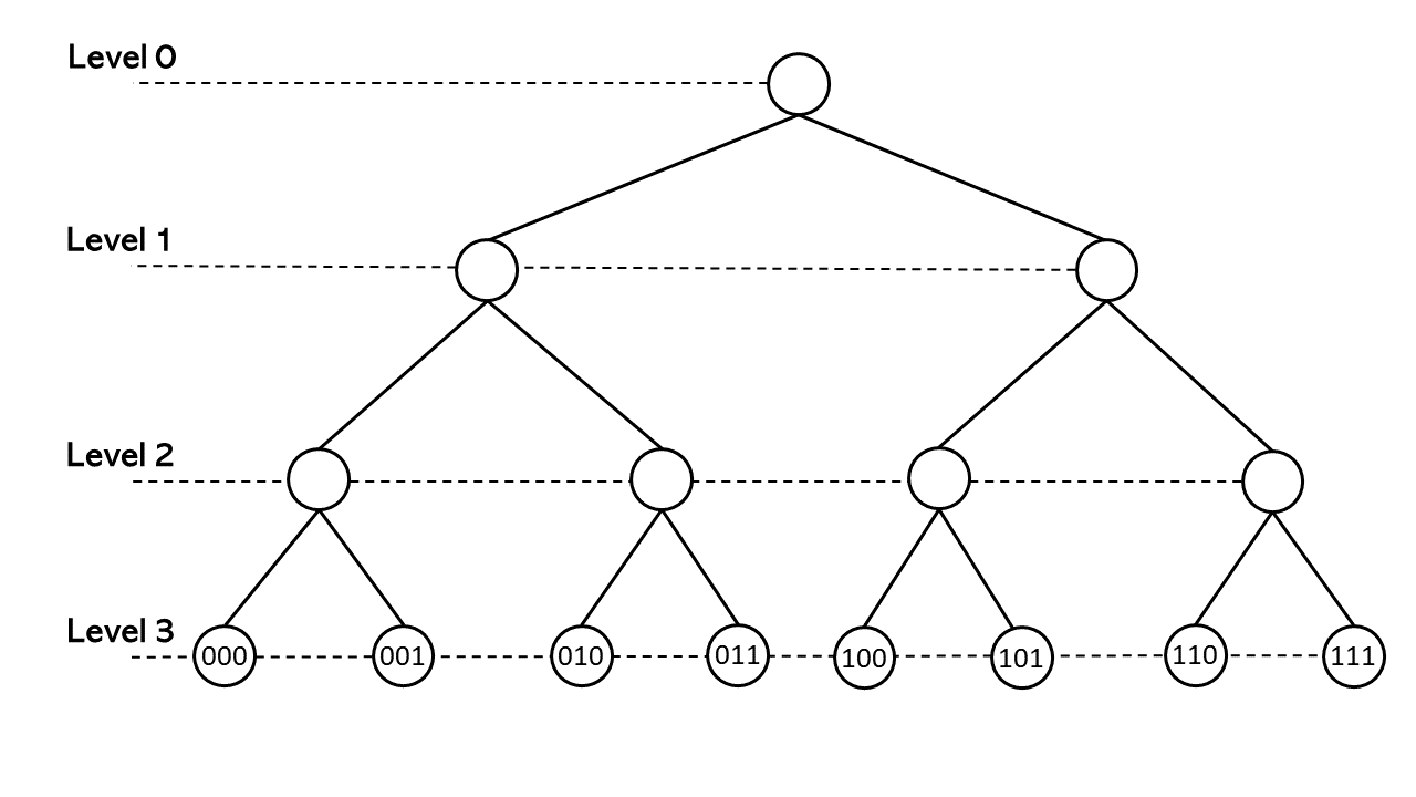
Figure 1: The rooted tree associated with the group $\mathbb{Z}_{2}/2^{3}\mathbb{Z}_{2}$. The elements of $\mathbb{Z}_{2}/2^{3}\mathbb{Z}_{2}$ have the form $i=i_{0}+i_{1}2+i_{2}2^{2}$,$\;i_{0}$, $i_{1}$, $i_{2}\in\{0,1\}$. The distance satisfies $-\log_{2}\left|i-j\right|_{2}=$level of the first common ancestor of $i$, $j$. Taken from [70].

The unit ball $\mathbb{Z}_{p}$ (which is the inverse limit of the $G_{l}$s) is an infinite rooted tree with fractal structure, see Figure 2.

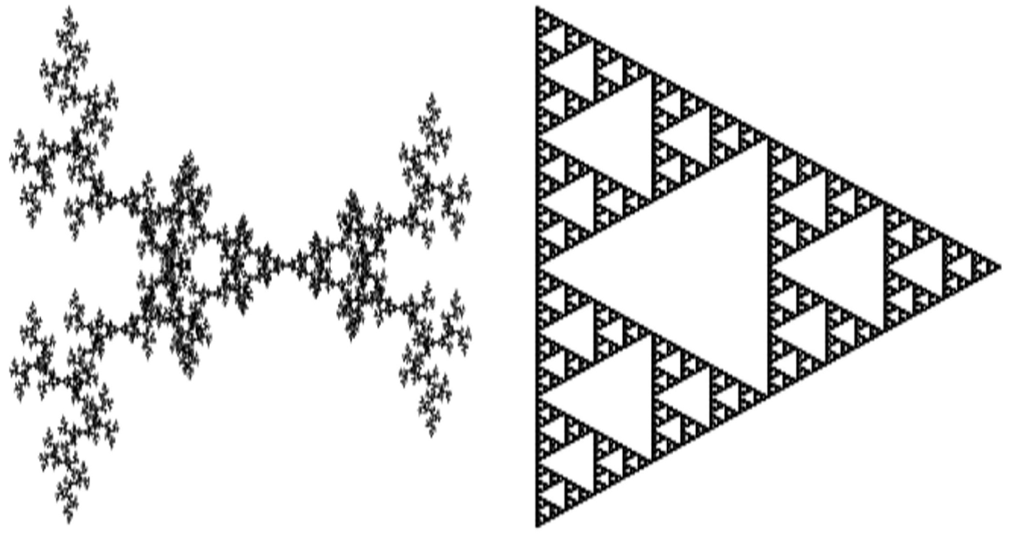
Figure 2: Based upon [73], construct an embedding $\mathfrak{f}:\mathbb{Z}_{\wp}\rightarrow\mathbb{R}^{2}$. The figure shows the images of $\mathfrak{f}(\mathbb{Z}_{2})$ and $\mathfrak{f}(\mathbb{Z}_{3})$. This computation requires a truncation of the $\wp$-adic integers. We use $\mathbb{Z}_{2}/2^{14}\mathbb{Z}_{2}$ and $\mathbb{Z}_{3}/3^{10}\mathbb{Z}_{3}$, respectively. Taken from [70].

We extend the $p-$adic norm to $\mathbb{Q}_{p}^{N}$ by taking

$$||x||_{p}:=\max_{1\leq i\leq N}|x_{i}|_{p},\qquad\text{for }x=(x_{1},\dots,x_{N})\in\mathbb{Q}_{p}^{N}.$$

We define $ord(x)=\min_{1\leq i\leq N}\{ord(x_{i})\}$, then $||x||_{p}=p^{-ord(x)}$. The metric space $\left(\mathbb{Q}_{p}^{N},||\cdot||_{p}\right)$ is a complete ultrametric space.

A function $\varphi:\mathbb{Q}_{p}^{N}\rightarrow\mathbb{C}$ is called locally constant, if for any $a\in\mathbb{Q}_{p}^{N}$, there is an integer $l=l(a)$, such that

$$\varphi\left(a+x\right)=\varphi\left(a\right)\text{ for any }||x||_{p}\leq p^{l}.$$

The set of functions for which $l=l\left(\varphi\right)$ depends only on $\varphi$ form a $\mathbb{C}$-vector space denoted as $\mathcal{U}_{loc}\left(\mathbb{Q}_{p}^{N}\right)$. We call $l\left(\varphi\right)$ the exponent of local constancy. If $\varphi\in\mathcal{U}_{loc}\left(\mathbb{Q}_{p}^{N}\right)$ has compact support, we say that $\varphi$ is a test function. We denote by $\mathcal{D}(\mathbb{Q}_{p}^{N})$ the complex vector space of test functions. There is a natural integration theory so that $\int_{\mathbb{Q}_{p}^{N}}\varphi\left(x\right)dx$ gives a well-defined complex number. The measure $d^{N}x$ is the Haar measure of $\mathbb{Q}_{p}^{N}$. In the Appendix (Section 11), we give a quick review of the basic aspects of the $p$-adic analysis required here.

The QM in the sense of the Dirac-von Neumann can be formulated on the Hilbert space

$$L^{2}(\mathbb{Q}_{p}^{N}):=L^{2}(\mathbb{Q}_{p}^{N},d^{N}x)=\left\{f:\mathbb{Q}_{p}^{N}\rightarrow\mathbb{C};\left\|f\right\|_{2}=\left(\mathop{\displaystyle\int}\limits_{\mathbb{Q}_{p}^{N}}\left|f\left(x\right)\right|d^{N}x\right)^{\frac{1}{2}}<\infty\right\}.$$

This space has a countable orthonormal basis, and thus $L^{2}(\mathbb{Q}_{p}^{N},d^{N}x)$ is isometric to $l_{2}(\mathbb{C})$. On the other hand, $L^{2}(\mathbb{R}^{N},d^{N}x)$, here $d^{N}x$ denotes the Lebesgue measure of $\mathbb{R}^{N}$, is also isometric to $l_{2}(\mathbb{C})$, and thus $L^{2}(\mathbb{R}^{N},d^{N}x)$ is isometric to $L^{2}(\mathbb{Q}_{p}^{N},d^{N}x)$. However, the first choice $L^{2}(\mathbb{R}^{N},d^{N}x)$ implies that the space ($\mathbb{R}^{N}$) is continuous, while in the second choice $L^{2}(\mathbb{Q}_{p}^{N},d^{N}x)$, the space ($\mathbb{Q}_{p}^{N}$) is a completely disconnected.

5 $p$-Adic  numbers in physics

Using $p$-adic numbers in physics raises several new questions. Here, we discuss two which are relevant in this work.

5.1 What is the role of $p$?

For the sake of simplicity, in order to discuss this matter we take $N=1$. The transformations of type

$$\rho_{a,L}:x\rightarrow a+p^{L}x\text{, with }a\in\mathbb{Q}_{p}\text{, }L\in\mathbb{Z},$$

constitute a scale group for the set $\mathbb{Q}_{p}\setminus\left\{0\right\}$. This set is self-similar, i.e.,

$$\mathbb{Q}_{p}\setminus\left\{0\right\}={\displaystyle\bigcup\limits_{a,L}}\rho_{a,L}\left(\mathbb{Q}_{p}\setminus\left\{0\right\}\right).$$

Given two different points $x_{1}$, $x_{2}$ in $\mathbb{Q}_{p}\setminus\left\{0\right\}$, we say that they are equivalent, denoted as $x_{1}\sim$ $x_{2}$, if $\rho_{a,L}\left(x_{1}\right)=x_{2}$, for some $\rho_{a,L}$. Then, any non-zero $p$-adic number

$$x=p^{ord(x)}{\displaystyle\sum\limits_{k=0}^{\infty}}x_{k}p^{k}=p^{ord(x)}ac\left(x\right)\text{, with }x_{0}\neq 0\text{ and }\left|ac\left(x\right)\right|_{p}=1$$

is equivalent to a point the the unit sphere

$$\mathbb{Z}_{p}^{\times}=\left\{x\in\mathbb{Z}_{p};\left|x\right|_{p}=1\right\},$$

and thus

$$\mathbb{Q}_{p}\setminus\left\{0\right\}={\displaystyle\bigsqcup\limits_{k=-\infty}^{\infty}}p^{k}\mathbb{Z}_{p}^{\times},$$

where ${\textstyle\bigsqcup}$ denotes  disjoint union.  Now,

$$\mathbb{Z}_{p}^{\times}={\displaystyle\bigsqcup\limits_{j_{0}=1}^{p-1}}{\displaystyle\bigsqcup\limits_{j_{1}=0}^{p-1}}\left(j_{0}+j_{1}p+p^{2}\mathbb{Z}_{p}\right)\text{,}$$

and by using a suitable transformation $\rho_{a,L}$ any element of the set $j_{0}+j_{1}p+p^{2}\mathbb{Z}_{p}$ is equivalent to $j_{0}+j_{1}p$. These elements form a rooted tree $T_{j_{0}}$, with root $j_{0}$, and one layer. The vertices on this layer correspond with the points of the form $j_{0}+j_{1}p$. In conclusion, $\mathbb{Q}_{p}\setminus\left\{0\right\}$ is a self-similar set with a tree-like structure, having the forest ${\textstyle\bigsqcup\nolimits_{j_{0}=1}^{p-1}}T_{j_{0}}$ as a fundamental domain for the action of the scale group action. Then, up to a scale transformation,  the smallest distance  between two points in $\mathbb{Q}_{p}\setminus\left\{0\right\}$ is

$$p^{-1}=\left|j_{0}-\left(j_{0}+j_{1}p\right)\right|_{p}.$$

We warn the reader about the following facts. If we consider the number $p$ as a real number $p=\left|p\right|$. But, if we consider $p$ as a $p$-adic number, $p\neq\left|p\right|_{p}=p^{-1}$. This phenomenon causes big trouble when using $p$-adic numbers in physics. We introduce the principle of the inaccessibility of $p$-adic numbers. Only the $p$-adic norm of the result of a computation using $p$-adic numbers can be compared against some measurable physical quantity.

5.2 Motion in a $p$-adic space

The product topology of $\mathbb{Q}_{p}^{N}\times\mathbb{R}_{+}$ imposes serious restrictions to the notion of motion. In classical physics the trajectory of a particle in $\mathbb{R}^{N}$ is a continuous curves contained in $\mathbb{R}^{N}$, i.e.,

$$\begin{array}[c]{ccc}\left[0,\infty\right)&\rightarrow&\mathbb{R}^{N}\\ &&\\ t&\rightarrow&X(t).\end{array}$$

In the $p$-adic case, the trajectories have the form

$$\begin{array}[c]{ccc}\left[0,\infty\right)&\rightarrow&\mathbb{Q}_{p}^{N}\\ &&\\ t&\rightarrow&Y(t).\end{array}$$

If the $Y$ is continuous, the image $Y(\left[0,\infty\right))$ should be a connected subset of $\mathbb{Q}_{p}^{N}$, since the only connected subsets of $\mathbb{Q}_{p}^{N}$ are the empty set, and the points, the function $Y$ should be constant. Therefore, the non-trivial trajectories are discontinuous curves. This mathematical result can be reformulated as the motion of a particle in $\mathbb{Q}_{p}^{N}$ is a sequence of jumps.

Suppose that $Y(t)\in\mathbb{Q}_{p}^{N}$ , $t\in\left[0,\infty\right)$, is the trajectory of a particle in $\mathbb{Q}_{p}^{N}$. Consider a function $F:$ $\mathbb{Q}_{p}^{N}\rightarrow\mathbb{C}$, then $F\left(Y(t)\right)\in\mathbb{C}$ is not the trajectory of particle in $\mathbb{Q}_{p}^{N}$. The function $F\left(Y(t)\right)$ is just a picture that may capture relevant features of a motion in $\mathbb{Q}_{p}^{N}$. For instance, linear combinations of functions of type $F\left(Y(t)\right)=\exp\left(2\pi if\left\|Y(t)\right\|\right)$, $f\in\mathbb{R}$, may produced  interference patterns in $\mathbb{C=R}^{2}$, but we cannot interpret theses patterns as produced by the interference of waves in $\mathbb{Q}_{p}^{N}$.

6 $p$-Adic heat equations and Markov processes

In this section, we review quickly the basic aspects of the $p$-adic heat equations. For an in-depth  discussion the reader may consult [8]-[9], and the references therein.

We denote by $\mathcal{C}(\mathbb{Q}_{p}^{N})$ the $\mathbb{C}$-vector space of continuous functions defined on $\mathbb{Q}_{p}^{N}$. The Taibleson-Vladimirov pseudodifferential operator $\boldsymbol{D}^{\alpha}$, $\alpha>0$, is defined as

$$\begin{array}[c]{cccc}\boldsymbol{D}^{\alpha}:&\mathcal{D}(\mathbb{Q}_{p}^{N})&\rightarrow&L^{2}(\mathbb{Q}_{p}^{N})\cap\mathcal{C}(\mathbb{Q}_{p}^{N})\\ &&&\\ &\varphi(x)&\rightarrow&\boldsymbol{D}^{\alpha}\varphi(x)=\mathcal{F}_{\xi\rightarrow x}^{-1}\left(||\xi||_{p}^{\alpha}\mathcal{F}_{x\rightarrow\xi}\left(\varphi\right)\right),\end{array}$$ (6.1)

where $\mathcal{F}$ denotes the Fourier transform, see the Appendix for the definition and further details about the Fourier transform on $\mathbb{Q}_{p}^{N}$. This operator admits an extension of the form

$$\left(\boldsymbol{D}^{\alpha}\varphi\right)\left(x\right)=\frac{1-p^{\alpha}}{1-p^{-\alpha-N}}\int\limits_{\mathbb{Q}_{p}^{N}}||y||_{p}^{-\alpha-N}(\varphi(x-y)-\varphi(x))\,d^{N}y$$

to the space of locally locally constant functions $\varphi(x)$ satisfying

$$\int\limits_{||x||_{p}\geq 1}||x||_{p}^{-\alpha-N}|\varphi(x)|\,d^{N}x<\infty.$$

In particular, the Taibleson-Vladimirov derivative of any order of a constant function is zero.

The equation

$$\frac{\partial u(x,t)}{\partial t}+\boldsymbol{D}^{\alpha}u(x,t)=0,\quad x\in\mathbb{Q}_{p}^{N},\quad t\geq 0$$

is called the $p$-adic heat equation. The heat kernel attached to the symbol $a||\xi||_{p}^{\alpha}$, $a>0$,  is defined as

$$Z(x,t)=\int\limits_{\mathbb{Q}_{p}^{N}}\chi_{p}(-x\cdot\xi)e^{-t||\xi||_{p}^{\alpha}}\,d^{N}\xi\text{, for }t>0\text{ \ and }x\in\mathbb{Q}_{p}^{N}.$$ (6.2)

Since $e^{-at||\cdot||_{p}^{\alpha}}\in L^{1}\left(\mathbb{Q}_{p}^{N}\right)$ for $t>0$, $Z(x,t)$ is a continuous function in $x\in\mathbb{Q}_{p}^{N}$ for $t>0$. The heat kernel has the following properties:

(i) $Z(x,t)\geq 0$, for all $x\in\mathbb{Q}_{p}^{N}$,$\quad t\in(0,\infty)$;

(ii) ${\textstyle\int\nolimits_{\mathbb{Q}_{p}^{N}}}Z\left(x,t\right)$ $d^{N}x=1$, for any $t>0$;

(iii) if $\varphi\in\mathcal{D}\left(\mathbb{Q}_{p}^{N}\right)$, then $\lim_{\left(x,t\right)\rightarrow\left(x_{0},0\right)}{\textstyle\int\nolimits_{\mathbb{Q}_{p}^{N}}}Z\left(x-\eta,t\right)\varphi\left(\eta\right)d^{N}\eta=\varphi\left(x_{0}\right)$;

(iv) $Z\left(x,t+t^{\prime}\right)={\textstyle\int\nolimits_{\mathbb{Q}_{p}^{N}}}Z\left(x-y,t\right)Z\left(y,t^{\prime}\right)d^{N}y$, for $t$, $t^{\prime}>0$,

see [8, Chaper 2,  Theorem 13]. In addition, the heat kernel $Z\left(x,t\right)$ is a transition density of a time homogeneous Markov process with discontinuous paths, [8, Chaper 2,  Theorem 16].

In $\mathbb{R}^{N}$, the fractional Laplacian is defined as $\widehat{\left(-\Delta f\right)^{\beta}}=\left|\xi\right|_{\mathbb{R}}^{\beta}\widehat{f}$, for $\beta\in\left[0,2\right]$, on the  Schwartz space, where $\widehat{\cdot}$ denotes the Fourier transform on $\mathbb{R}^{N}$, see [8, Chaper 4], and the references therein. The fractional heat equation in $\mathbb{R}^{N}$ is

$$\frac{\partial u(x,t)}{\partial t}+a\left(-\Delta f\right)^{\beta}u(x,t)=0,\quad x\in\mathbb{R}^{N},\quad t\geq 0,$$

with $a>0$. There are ‘more’ $p$-adic heat equations than Archimedean ones, see [8, Chapter 4]. For instance, the $p$-adic heat equations  with variable coefficients presented in [8, Chapter 3] do not have Archimedean counterparts. All the $p$-adic Laplacians are non-local operators, in addition, they can be combined with the Archimedean fractional Laplacian into an adelic operator, and the corresponding adelic heat equation is associated with a Markov process whose state space the ring of adeles, see [8, Chapter 4, Theorem 123].

7 $p$-Adic Schrödinger equations

A large class $p$-adic quantum mechanics is obtained from the Dirac-von Neumann formulation by taking $\mathcal{H}=L^{2}(\mathbb{Q}_{p}^{N})$. A specific Schrödinger equation controls the dynamic evolution of the quantum states in each particular QM. Such an equation is obtained from a $p$-adic heat by the Wick rotation. We select the simplest possible heat equation:

$$\frac{\partial\Psi(x,t)}{\partial t}=-\boldsymbol{D}^{\alpha}\Psi(x,t),\quad x\in\mathbb{Q}_{p}^{N},\quad t\geq 0,$$ (7.1)

where $\boldsymbol{D}^{\alpha}$ is the Taibleson-Vladimirov pseudo-differential operator. By performing the Wick rotation $t\rightarrow it$, where $i=\sqrt{-1}$, (7.1) becomes

$$i\frac{\partial\Psi(x,t)}{\partial t}=\boldsymbol{D}^{\alpha}\Psi(x,t)=0,\quad x\in\mathbb{Q}_{p}^{N},\quad t\geq 0.$$ (7.2)

We propose the following Schrödinger equation for a single nonrelativistic particle with mass $m$ moving in $\mathbb{Q}_{p}^{N}$ under a potential $V(x,t)$:

$$i\hbar\frac{\partial\Psi(x,t)}{\partial t}=\left\{\frac{\hbar^{2}}{2m}\boldsymbol{D}^{\alpha}+V(x,t)\right\}\Psi(x,t)\text{, }x\in\mathbb{Q}_{p}^{N},\quad t\geq 0.$$ (7.3)

If $\frac{\hbar^{2}}{2m}=1$ and $V(x,t)=0$, then equation (7.3) becomes (7.2). For the rest of the section, we assume that $\frac{\hbar^{2}}{2m}=1$ and that $V(x)$ is time-independent. The Schrödinger operators $\boldsymbol{D}^{\alpha}+V(x)$ has been extensively studied, see, e.g., [7, Chapter 3], [6, Chapter 2.], [82].

7.1 Time evolution operators

We recall that a function $V:\mathbb{Q}_{p}^{N}\rightarrow\mathbb{R}$ is called locally bounded, if for any $x_{0}\in\mathbb{Q}_{p}^{N}$, there exists a neighborhood $\mathcal{N}$ of $x_{0}$ and a positive constant $M$ such that

$$\left|f\left(x\right)\right|\leq M\text{ for all }x\in\mathcal{N}.$$

Let $V:\mathbb{Q}_{p}^{N}\rightarrow\mathbb{R}$ be a locally bounded, measurable function. Define the operator $\boldsymbol{H}^{\prime}$ on $L^{2}(\mathbb{Q}_{p}^{N})$ with domain $D(\boldsymbol{H}^{\prime})=\mathcal{D}(\mathbb{Q}_{p}^{N})$ setting

$$\boldsymbol{H}^{\prime}\varphi\left(x\right)=\left(\boldsymbol{D}^{\alpha}+V(x)\right)\varphi\left(x\right).$$

Since $\mathcal{D}(\mathbb{Q}_{p}^{N})$ is dense in $L^{2}(\mathbb{Q}_{p}^{N})$ and $\boldsymbol{D}^{\alpha}\varphi\left(x\right)$, $V(x)\varphi\left(x\right)\in L^{2}(\mathbb{Q}_{p}^{N})$, see (6.1), $\boldsymbol{H}^{\prime}$ is a densely defined and symmetric operator. We denote by $\boldsymbol{H}$ its closure. This operator  is self-adjoint [7, Theorem 3.2]. Then, by Stone’s theorem, $e^{-it\boldsymbol{H}}$ is a unitary group on $L^{2}(\mathbb{Q}_{p}^{N})$  and

$$\Psi(x,t)=e^{-it\boldsymbol{H}}\Psi_{0}(x)\text{, for }t\in\mathbb{R}\text{, and }\Psi_{0}(x)\in L^{2}(\mathbb{Q}_{p}^{N})\text{,}$$

is the solution of the Cauchy problems attached to the $p$-adic Schrödinger equation with initial datum $\Psi_{0}$. In [22], [29], [31], Feynman-Kac formulas for the semigroups $e^{-it\boldsymbol{H}}$ for large class of potentials were established.

7.2 A Cauchy problem

We now consider the following Cauchy problem:

$$\left\{\begin{array}[c]{ll}\Psi(\cdot,t)\in\mathcal{C}\left(\left[0,\infty\right),\mathcal{D}(\mathbb{Q}_{p}^{N})\right);&\Psi(\cdot,t)\in\mathcal{C}^{1}\left(\left[0,\infty\right),L^{2}(\mathbb{Q}_{p}^{N})\right)\\ &\\ \frac{\partial\Psi(x,t)}{\partial t}=-i\boldsymbol{D}^{\alpha}\Psi(x,t),&x\in\mathbb{Q}_{p}^{N}\text{, }t\geq 0\\ &\\ \Psi(x,0)=\Psi_{0}(x)\in\mathcal{D}(\mathbb{Q}_{p}^{N}).&\end{array}\right.$$ (7.4)

By taking Fourier transform in the space variables, the solution of the evolution equation in (7.4) is given by

$$\widehat{\Psi}(\xi,t)=\widehat{\Psi}_{0}(\xi)e^{-it||\xi||_{p}^{\alpha}},$$

now, since $\widehat{\Psi}_{0}(\xi)\in\mathcal{D}(\mathbb{Q}_{p}^{N})$ and $e^{-it||\xi||_{p}^{\alpha}}\in\mathcal{C}(\mathbb{Q}_{p}^{N})$, it verifies that

$$\widehat{\Psi}_{0}(\xi)e^{-it||\xi||_{p}^{\alpha}}\in L^{1}(\mathbb{Q}_{p}^{N})\cap L^{2}(\mathbb{Q}_{p}^{N})\text{, for }t\geq 0,$$

and consequently

$$\Psi(x,t)={\displaystyle\int\limits_{\mathbb{Q}_{p}^{N}}}\chi_{p}\left(-\xi\cdot x\right)\widehat{\Psi}_{0}(\xi)e^{-it||\xi||_{p}^{\alpha}}d^{N}\xi\in\mathcal{C}(\mathbb{Q}_{p}^{N})\cap L^{2}(\mathbb{Q}_{p}^{N})\text{, for }t\geq 0.$$ (7.5)

Now considering $\Psi(\cdot,t)$, $t\in\mathbb{R}$, as a distribution from $\mathcal{D}^{\prime}(\mathbb{Q}_{p}^{N})$, sse the Appendix, and since $e^{-it||\xi||_{p}^{\alpha}}\in L_{loc}^{1}(\mathbb{Q}_{p}^{N})$, we have

$$\Psi(x,t)=\mathcal{F}_{\xi\rightarrow x}^{-1}(e^{-it||\xi||_{p}^{\alpha}})\ast\Psi_{0}(x).$$

Furthermore,

$$\mathcal{F}_{\xi\rightarrow x}^{-1}(e^{-it||\xi||_{p}^{\alpha}})=Z(x,it)\text{ in }\mathcal{D}^{\prime}(\mathbb{Q}_{p}^{N})\text{, for }t\geq 0,$$

where $Z(x,t)$ is the heat kernel defined in (6.2). This last equality follows from the fact that the Fourier transform is a homeomorphism on $\mathcal{D}^{\prime}(\mathbb{Q}_{p}^{N})$. In conclusion, for $\Psi_{0}(x)\in\mathcal{D}(\mathbb{Q}_{p}^{N})$,

$$\Psi(x,t)=Z(x,it)\ast\Psi_{0}(x)=e^{-it\boldsymbol{H}}\Psi_{0}(x)\in\mathcal{C}(\mathbb{Q}_{p}^{N})\cap L^{2}(\mathbb{Q}_{p}^{N}),$$

for $t\geq 0$.

7.3 Born interpretation of the wave function

Assume that

$${\displaystyle\int\limits_{\mathbb{Q}_{p}^{N}}}\left|\Psi_{0}(x)\right|^{2}d^{N}x=1,$$ (7.6)

and set $\varrho\left(x,t\right):=\left|\Psi(x,t)\right|^{2}$. The interpretation of solution $\Psi(x,t)$ is that

$${\displaystyle\int\limits_{E}}\varrho\left(x,t\right)d^{N}x$$

is the probability of finding a single particle in the (Borel) subset $E\subset\mathbb{Q}_{p}^{N}$ at the time $t$. Notice that by using the fact that the Fourier transform preserves the inner product in $L^{2}(\mathbb{Q}_{p}^{N})$, we have

$${\displaystyle\int\limits_{\mathbb{Q}_{p}^{N}}}\varrho\left(x,t\right)d^{N}x ={\displaystyle\int\limits_{\mathbb{Q}_{p}^{N}}}\Psi(x,t)\overline{\Psi(x,t)}d^{N}x={\displaystyle\int\limits_{\mathbb{Q}_{p}^{N}}}\widehat{\Psi}(\xi,t)\overline{\widehat{\Psi}(\xi,t)}d^{N}\xi$$

$$={\displaystyle\int\limits_{\mathbb{Q}_{p}^{N}}}\left|\widehat{\Psi_{0}}(\xi)\right|^{2}d^{N}\xi=1.$$

8 de Broglie Wave-particle duality

8.1 The classical case

1923 de Broglie postulates the existence of a correspondence between a beam of free particles with momentum $\mathsf{p}$ and energy $\mathsf{E}$ with a wave of form

$$\psi_{\mathbb{R}}\left(x,t\right)=Ae^{i\left(\kappa\cdot x-\omega t\right)}\text{, \ \ \ }k\in\mathbb{R}^{N}\text{, }\left(x,t\right)\in\mathbb{R}^{N+1}.$$ (8.1)

A such correspondence should be relativistic so $\kappa\cdot x-\omega t$ is a Lorentz invariant scalar product, which implies that the vectors $\left(\mathsf{p},\mathsf{E}\right)$ and $\left(\kappa,\omega\right)$ should be proportional, see, e.g., [5, pp 36-37]. Now, by the Planck-Einsten law $\mathsf{E}=\hbar\omega$, which implies that $\left(\mathsf{p},\mathsf{E}\right)=\hbar\left(\kappa,\omega\right)$. The particle wavelength is

$$\lambda=\frac{2\pi}{\left|\kappa\right|}=\frac{2\pi\hbar}{\left|\mathsf{p}\right|}.$$

Since the plane waves (8.1) are solutions of the free Schrödinger equation; the de Broglie waves are ‘quantum waves.’ We now discuss these matters in the $p$-adic framework.

8.2 The $p$-adic case

Before discussing the de Broglie Wave-particle duality in the $p$-adic framework, we require some preliminary results.

8.2.1 Additive characters

We recall that $p$-adic number $x\neq 0$ has a unique expansion of the form $x=p^{ord(x)}\sum_{j=0}^{\infty}x_{j}p^{j},$ where $x_{j}\in\{0,\dots,p-1\}$ and $x_{0}\neq 0$. By using this expansion, we define the fractional part of $x\in\mathbb{Q}_{p}$, denoted $\{x\}_{p}$, as the rational number

$$\left\{x\right\}_{p}=\left\{\begin{array}[c]{lll}0&\text{if}&x=0\text{ or }ord(x)\geq 0\\ &&\\ p^{ord(x)}\sum_{j=0}^{-ord(x)-1}x_{j}p^{j}&\text{if}&ord(x)<0.\end{array}\right.$$

Set $\chi_{p}(y)=\exp(2\pi i\{y\}_{p})$ for $y\in\mathbb{Q}_{p}$. The map $\chi_{p}(\cdot)$ is an additive character on $\mathbb{Q}_{p}$, i.e., a continuous map from $\left(\mathbb{Q}_{p},+\right)$ into $S$ (the unit circle considered as multiplicative group) satisfying $\chi_{p}(x_{0}+x_{1})=\chi_{p}(x_{0})\chi_{p}(x_{1})$, $x_{0},x_{1}\in\mathbb{Q}_{p}$.  The additive characters of $\mathbb{Q}_{p}$ form an Abelian group which is isomorphic to $\left(\mathbb{Q}_{p},+\right)$. The isomorphism is given by $\xi\rightarrow\chi_{p}(\xi x)$, see, e.g., [75, Section 2.3].

8.2.2 $p$-Adic wavelets

Given $\xi=\left(\xi_{1},\ldots,\xi_{N}\right)$, $x=\left(x_{1},\ldots,x_{N}\right)\in\mathbb{Q}_{p}^{N}$, we set $\xi\cdot x=\sum_{i=1}^{N}\xi_{i}x_{i}$. We denote by $\Omega\left(p^{L}\left\|x-a\right\|_{p}\right)$ the characteristic function of the ball

$$B_{-L}^{N}(a)=\left\{x\in\mathbb{Q}_{p}^{N};\left\|x-a\right\|_{p}\leq p^{-L}\right\}=a+p^{L}\mathbb{Z}_{p}^{N}.$$

We now define

$$\mathbb{Q}_{p}/\mathbb{Z}_{p}=\left\{\sum_{j=-1}^{-m}x_{j}p^{j};\text{for some }m>0\right\}.$$

For $b=\left(b_{1},\ldots,b_{N}\right)\in\left(\mathbb{Q}_{p}/\mathbb{Z}_{p}\right)^{N}$, $r\in\mathbb{Z}$, we denote by $\Omega\left(\left\|p^{r}x-b\right\|_{p}\right)$ the characteristic function of the ball $bp^{-r}+p^{-r}\mathbb{Z}_{p}^{N}$.

Set

$$\Psi_{rbk}\left(x\right)=p^{\frac{-rN}{2}}\chi_{p}(p^{-1}k\cdot\left(p^{r}x-b\right))\Omega\left(\left\|p^{r}x-b\right\|_{p}\right),$$ (8.2)

where $r\in\mathbb{Z}$, $k=\left(k_{1},\ldots,k_{N}\right)\in\{0,\dots,p-1\}^{N}$, $k\neq\left(0,\ldots,0\right)$, and $b=\left(b_{1},\ldots,b_{N}\right)\in\left(\mathbb{Q}_{p}/\mathbb{Z}_{p}\right)^{N}$. With this notation,

$$\boldsymbol{D}^{\alpha}\Psi_{rbk}\left(x\right)=p^{\left(1-r\right)\alpha}\Psi_{rnk}\left(x\right)\text{, for any }r,n,k.$$ (8.3)

Moreover,

$${\displaystyle\int\limits_{\mathbb{Q}_{p}^{N}}}\Psi_{rbk}\left(x\right)d^{N}x=0,$$ (8.4)

and $\left\{\Psi_{rnk}\left(x\right)\right\}_{rbk}$ forms a complete orthonormal basis of $L^{2}(\mathbb{Q}_{p}^{N})$, see, e.g., [75, Theorems 9.4.5 and 8.9.3], [76, Theorem 3.3].

The wavelets $\Psi_{rbk}$ are obtained from the mother wavelet

$$\Psi_{k}\left(x\right)=\chi_{p}(p^{-1}k\cdot x)\Omega\left(\left\|x\right\|_{p}\right)$$

as an orbit of the action of the group $x\rightarrow-n+p^{r}x$, $\Psi_{rbk}\left(x\right)=p^{\frac{-Nr}{2}}\Psi_{k}\left(-n+p^{r}x\right)$, see [Alberio-Kozyrev]. The constant $p^{\frac{-Nr}{2}}$ is a normalization factor so $\left\|\Psi_{rbk}\right\|_{2}=1$.

8.2.3 $p$-Adic plane waves

We now investigate the existence of plane waves for the free Schrödinger equation $i\frac{\partial\Psi(x,t)}{\partial t}=\boldsymbol{D}^{\alpha}\Psi(x,t)$. By separating variables as $\Psi(x,t)=\Psi_{time}(t)\Psi_{space}(x)$ and using (8.3), we have

$$i\frac{\Psi_{time}^{\prime}(t)}{\Psi_{time}(t)}=\frac{\boldsymbol{D}^{\alpha}\Psi_{space}(x)}{\Psi_{space}(x)}=\omega,$$

and thus

$$\Psi(x,t) =e^{-ip^{\left(1-r\right)\alpha}t}\Psi_{rnk}\left(x\right)$$

$$=A\exp\left\{-i\left(p^{\left(1-r\right)\alpha}t-2\pi\left\{p^{r-1}k\cdot x\right\}_{p}\right)\right\}\Omega\left(\left\|p^{r}x-b\right\|_{p}\right)\text{, }\left(x,t\right)\in\mathbb{Q}_{p}^{N}\times\mathbb{R},$$ (8.5)

where $\omega=p^{\left(1-r\right)\alpha}$, and $A=A(k,b)\in\mathbb{C}$. The quantity $p^{\left(1-r\right)\alpha}$ is an angular frequency, since it is discrete, we postulate that the energy of wave (8.5) is

$$\mathsf{E}=\hbar p^{\left(1-r\right)\alpha}.$$

8.3 $p$-Adic de Broglie waves

In standard QM the de Broglie waves are the plane wave solutions of the Schrödinger equation. By analogy, in the $p$-adic case, the de Broglie waves have the form (8.5). There are two central differences between the $p$-adic case and the standard one. First, the scale group of $\mathbb{Q}_{p}^{N}$ acts naturally on the plane waves (8.5) such as we explained at the end of Section 8.2.2. Second,

$$\text{all the }p\text{-adic planes waves (\ref{Plane_Waves_2}) have wavelength }p^{-1}\text{.}$$ (8.6)

This result implies that the de Broglie wave-particle duality does not hold in the $p$-adic framework. It is an expected result since the smallest distance in $\mathbb{Q}_{p}^{N}$ up to a scale transformation is $p^{-1}$. On the other hand, To verify (8.6), we first notice that the wavelength of (8.5) is determined by $\Psi_{rnk}\left(x\right)$, more precisely, by

$$\chi_{p}(p^{-1}k\cdot\left(p^{r}x-b\right))\text{, for }x\in p^{-r}b+p^{-r}\mathbb{Z}_{p}^{N}.$$

By writing, $p^{r}x-b=j+p\mathbb{Z}_{p}^{N}$, where $j=j(x)\in\left\{0,\ldots,p-1\right\}^{N}$, and using that the restriction of $\chi_{p}$ to the unit ball is constanthet function $1$, we have

$$\chi_{p}(p^{-1}k\cdot\left(p^{r}x-b\right)) =\chi_{p}(p^{-1}k\cdot j)\chi_{p}(k\cdot\mathbb{Z}_{p}^{N})=\chi_{p}(p^{-1}k\cdot j)=\chi_{p}(p^{-1}{\textstyle\sum\limits_{i=1}^{N}}k_{i}j_{i})$$

$$=\exp\left(2\pi i\left\{p^{-1}{\textstyle\sum\limits_{i=1}^{N}}k_{i}j_{i}\right\}_{p}\right)=\exp\left(i\frac{2\pi}{p}{\textstyle\sum\limits_{i=1}^{N}}k_{i}j_{i}\right),$$ (8.7)

where in the last equality we use the convention that $k_{i}$, $j_{i}$ are integers $\operatorname{mod}$ $p$, so the sum

$${\textstyle\sum\limits_{i=1}^{N}}k_{i}j_{i}\in\left\{0,\ldots,p-1\right\}.$$

In this calculation $p\in\mathbb{Q}_{p}$, then the wavelength of (8.7) is $\left|p\right|_{p}=p^{-1}$.

By using the conclusions of the discussion about the motion in $\mathbb{Q}_{p}^{N}$ given at the end of Section 5.2, we have

$$\text{the }p\text{-adic de Broglie waves are not physical but just mathematical objects.}$$ (8.8)

9 The $p$-adic Schrödinger equation with Gaussian initial data

Our next goal is to study the two-slit experiment in the framework of the $p$-adic QM. A key ingredient is a $p$-adic notion of Gaussian random variables. Here, we use the notion of $\mathbb{Q}_{p}$-Gaussian $\mathbb{Q}_{p}$-valued random variables introduced by Evans, [77], see also [7, Chapter 6]. A $p$-adic valued random variable $Y$ that is not almost surely zero is $\mathbb{Q}_{p}$-Gaussian if and only if its distribution is a cutoff of the Haar measure:

$$\mathbb{P}(Y\in d^{N}x)=p^{-mN}\Omega\left(p^{-m}\left\|x\right\|_{p}\right)d^{N}x$$ (9.1)

for some $m\in\mathbb{Z}$, or equivalently

$$E(\chi_{p}\left(\xi\cdot Y\right))=\Omega\left(p^{m}\left\|\xi\right\|_{p}\right)\text{, \ }\xi\in\mathbb{Q}_{\mathfrak{p}}^{N},$$

where $\Omega$ is the characteristic function of the interval $\left[0,1\right]$, see [7, Theorem 6.1].

Notice that

$$p^{-mN}\Omega\left(p^{-m}\left\|x\right\|_{p}\right)\text{ \ }\underrightarrow{\mathcal{F}_{x\rightarrow\xi}}\text{ \ }\Omega\left(p^{m}\left\|\xi\right\|_{p}\right)\text{, }m\in\mathbb{Z},$$

in particular, $\mathcal{F}_{x\rightarrow\xi}\left(\Omega\left(\left\|x\right\|_{p}\right)\right)=\Omega\left(\left\|\xi\right\|_{p}\right)$. We interpret the probability measure (9.1) as a Gaussian localized particle.

9.1 One-slit with Gaussian initial data

9.1.1 Some initial remarks

We assume that at time $T$, without loss of generality, we assume $T=0$, there is a Gaussian localized particle confined in the ball $p^{L}\mathbb{Z}_{p}^{N}$, $L\geq 0$. We interpret the ball $p^{L}\mathbb{Z}_{p}^{N}$ as a small slit around the origin. Following the classical formulation, see, e.g., [78]-[80] and the references therein, it is natural to propose the following Gaussian initial datum:

$$\Psi_{0}\left(x\right)=p^{\frac{LN}{2}}\Omega\left(p^{L}\left\|x\right\|_{p}\right)\chi_{p}\left(-k\cdot x\right)\text{, }$$

where $L$ is a non-negative integer and $k\in\mathbb{Q}_{p}^{N}$. Notice that $\Psi_{0}\left(x\right)\in\mathcal{D}(\mathbb{Q}_{p}^{N})$ satisfies normalization condition (7.6). Furthermore, if $k\in p^{-L}\mathbb{Z}_{p}^{N}$, i.e. $\left\|k\right\|_{p}\leq p^{L}$, since $x\in p^{L}\mathbb{Z}_{p}^{N}$, i.e. $\left\|x\right\|_{p}\leq p^{-L}$, $k\cdot x\in\mathbb{Z}_{p}$ and thus $\chi_{p}\left(k\cdot x\right)\equiv 1$. If $\left\|k\right\|_{p}>p^{L}$, then $\Psi_{0}\left(x\right)$ is a character of the additive group $p^{L}\mathbb{Z}_{p}^{N}$, which is an eigenfunction of $\boldsymbol{D}^{\alpha}$:

$$\boldsymbol{D}^{\alpha}\Psi_{0}\left(x\right)=||k||_{p}^{\alpha}\Psi_{0}\left(x\right).$$

This formula follows directly from the fact that

$$\widehat{\Psi}_{0}\left(\xi\right)=p^{\frac{-LN}{2}}\Omega\left(p^{-L}\left\|\xi-k\right\|_{p}\right).$$

The solution of Cauchy problem (7.4) with initial datum $\widehat{\Psi}_{0}\left(\xi\right)$ is

$$\Psi\left(x,t\right) =p^{-\frac{LN}{2}}{\displaystyle\int\limits_{\mathbb{Q}_{p}^{N}}}\chi_{p}\left(-\xi\cdot x\right)e^{-it||\xi||_{p}^{\alpha}}\Omega\left(p^{-L}\left\|\xi-k\right\|_{p}\right)d^{N}\xi$$

$$=p^{\frac{-LN}{2}}{\displaystyle\int\limits_{k+p^{-L}\mathbb{Z}_{p}^{N}}}\chi_{p}\left(-\xi\cdot x\right)e^{-it||\xi||_{p}^{\alpha}}d^{N}\xi,$$

see (7.5). We now change variables as

$$\xi=k+p^{-L}y\text{, \ }d^{N}\xi=p^{LN}d^{N}y,$$

and by the ultrametric property of the norm $||\cdot||_{p}$, $||k+p^{-L}y||_{p}^{\alpha}=||k||_{p}^{\alpha}$ for $\left\|k\right\|_{p}>p^{L}$ and any $\left\|y\right\|_{p}\leq 1$, then

$$\Psi\left(x,t\right) =p^{\frac{LN}{2}}\chi_{p}\left(-x\cdot k\right){\displaystyle\int\limits_{\mathbb{Z}_{p}^{N}}}\chi_{p}\left(-p^{-L}y\cdot x\right)e^{-it||k+p^{-L}y||_{p}^{\alpha}}d^{N}y$$

$$=p^{\frac{LN}{2}}\chi_{p}\left(-x\cdot k\right)e^{-it||k||_{p}^{\alpha}}{\displaystyle\int\limits_{\mathbb{Z}_{p}^{N}}}\chi_{p}\left(-p^{-L}y\cdot x\right)d^{N}y$$

$$=p^{\frac{LN}{2}}\chi_{p}\left(-x\cdot k\right)e^{-it||k||_{p}^{\alpha}}\Omega\left(\left\|p^{-L}x\right\|_{p}\right)=e^{-it||k||_{p}^{\alpha}}\Psi_{0}\left(x\right).$$

Therefore,

$$\left|\Psi\left(x,t\right)\right|^{2}=\left|\Psi_{0}\left(x\right)\right|.$$

In this case the particle remains confined in the ball $p^{L}\mathbb{Z}_{p}^{N}$. Due to this reason, we do not use phase factors of the form $\chi_{p}\left(-k\cdot x\right)$ in the initial datum.

9.1.2 Single-slit diffraction

Taking the considerations of the previous section, we set

$$\Psi_{0}\left(x\right)=p^{\frac{LN}{2}}\Omega\left(p^{L}\left\|x\right\|_{p}\right),$$

where $L$ is a non-negative integer. The solution of Cauchy problem (7.4) with initial datum $\widehat{\Psi}_{0}\left(\xi\right)=p^{\frac{-LN}{2}}\Omega\left(p^{-L}\left\|\xi\right\|_{p}\right)$ is

$$\Psi^{\left(1-slit\right)}\left(x,t\right) =p^{\frac{-LN}{2}}{\displaystyle\int\limits_{\mathbb{Q}_{p}^{N}}}\chi_{p}\left(-\xi\cdot x\right)e^{-it||\xi||_{p}^{\alpha}}\Omega\left(p^{-L}\left\|\xi\right\|_{p}\right)d^{N}\xi$$

$$=p^{\frac{-LN}{2}}{\displaystyle\int\limits_{p^{-L}\mathbb{Z}_{p}^{N}}}\chi_{p}\left(-\xi\cdot x\right)e^{-it||\xi||_{p}^{\alpha}}d^{N}\xi.$$ (9.2)

Diffraction pattern near to the origin

For $\left\|x\right\|_{p}\leq p^{-L}$,

$$\left|\Psi^{\left(1-slit\right)}\left(x,t\right)\right|^{2}\text{ is independent of }x\text{, and thus there is no a spatial diffraction pattern.}$$ (9.3)

To establish this result, we first set

$$\Psi_{0}^{\left(1-slit\right)}\left(x,t\right)=\Psi^{\left(1-slit\right)}\left(x,t\right)\Omega\left(p^{L}\left\|x\right\|_{p}\right).$$

The condition $\left\|x\right\|_{p}\leq p^{-L}$ implies that $x=p^{L}\widetilde{x}$, with $\left\|\widetilde{x}\right\|_{p}=1$. Since $\xi=p^{-L}\widetilde{\xi}$, with $\left\|\widetilde{\xi}\right\|_{p}=1$, we have $\xi\cdot x\in\mathbb{Z}_{p}$ thus $\chi_{p}\left(-\xi\cdot x\right)=1$, and

$$\Psi_{0}^{\left(1-slit\right)}\left(x,t\right)=p^{\frac{-LN}{2}}{\displaystyle\int\limits_{p^{-L}\mathbb{Z}_{p}^{N}}}e^{-it||\xi||_{p}^{\alpha}}d^{N}\xi.$$

By using the partition

$$p^{-L}\mathbb{Z}_{p}^{N}={\displaystyle\bigsqcup\limits_{j=-L}^{\infty}}p^{j}S_{0}^{N},$$ (9.4)

where $S_{0}^{N}=\left\{u\in\mathbb{Z}_{p}^{N};\left\|u\right\|_{p}=1\right\}$, we have

$$\Psi_{0}^{\left(1-slit\right)}\left(x,t\right) =p^{\frac{-LN}{2}}{\displaystyle\sum\limits_{j=-L}^{\infty}}\text{ }e^{-itp^{-j\alpha}}{\displaystyle\int\limits_{||\xi||_{p}=p^{-j}}}d^{N}\xi=p^{\frac{-LN}{2}}\left(1-p^{-N}\right){\displaystyle\sum\limits_{j=-L}^{\infty}}\text{ }e^{-itp^{-j\alpha}}p^{-jN}$$

$$=p^{\frac{-LN}{2}}\left(1-p^{-N}\right)\left\{{\displaystyle\sum\limits_{j=-L}^{\infty}}p^{-jN}\cos\left(p^{-j\alpha}t\right)+i{\displaystyle\sum\limits_{j=-L}^{\infty}}p^{-jN}\sin\left(p^{-j\alpha}t\right)\right\}.$$ (9.5)

Which shows that the diffraction pattern near the origin is independent of $x$.

Remark 9.1

By using that

$$\left|{\displaystyle\sum\limits_{j=1}^{\infty}}p^{-jN}\cos\left(p^{-j\alpha}t\right)+i{\displaystyle\sum\limits_{j=1}^{\infty}}p^{-jN}\sin\left(p^{-j\alpha}t\right)\right|\leq\frac{p^{-N}}{1-p^{-N}},$$

for any $t\geq 0$, one get the following approximation for $\Psi_{0}^{\left(1-slit\right)}\left(x,t\right)$:

$$\Psi_{0}^{\left(1-slit\right)}\left(x,t\right)\approx p^{\frac{-LN}{2}}\left(1-p^{-N}\right)\left\{{\displaystyle\sum\limits_{j=-L}^{0}}p^{-jN}\cos\left(p^{-j\alpha}t\right)+i{\displaystyle\sum\limits_{j=-L}^{0}}p^{-jN}\sin\left(p^{-j\alpha}t\right)\right\},$$

for $p$ sufficiently large. Then

$$\left|\Psi_{0}^{\left(1-slit\right)}\left(x,t\right)\right|^{2} \approx p^{-LN}\left(1-p^{-N}\right)^{2}\times$$

$$\left\{\left({\displaystyle\sum\limits_{j=0}^{L}}p^{jN}\cos\left(p^{j\alpha}t\right)\right)^{2}+\left({\displaystyle\sum\limits_{j=0}^{L}}p^{jN}\sin\left(p^{j\alpha}t\right)\right)^{2}\right\}$$

$$=p^{-LN}\left(1-p^{-N}\right)^{2}\left\{L+1+{\displaystyle\sum\limits_{j=0}^{L}}\text{ }{\displaystyle\sum\limits_{0\leq j<k\leq L}}\text{ }p^{\left(j+k\right)N}\cos\left(t\left(p^{j\alpha}-p^{k\alpha}\right)\right)\right\},$$ (9.6)

for $p$ sufficiently large.

Diffraction pattern at infinity

For $p$ sufficiently large, the diffraction pattern has the form

$$\left|\Psi^{\left(1-slit\right)}\left(x,t\right)\right|^{2}\approx\frac{4p^{-LN}}{\left\|x\right\|_{p}^{2N}}\sin^{2}\left(\frac{t\left(1-p^{\alpha}\right)}{2\left\|x\right\|_{p}^{\alpha}}\right)\text{,}$$ (9.7)

for$\ t>0$, $\left\|x\right\|_{p}>p^{-L}$. Furthermore,

$$\left|\Psi^{\left(1-slit\right)}\left(x,t\right)\right|^{2}\leq\frac{4p^{-LN}}{\left\|x\right\|_{p}^{2N}}\text{ for }t\geq 0\text{ and }\left\|x\right\|_{p}>p^{-L}\text{.}$$ (9.8)

This formula is established as follows. We set

$$\Psi_{\infty}^{\left(1-slit\right)}\left(x,t\right)=\Psi\left(x,t\right)\left(1-\Omega\left(p^{L}\left\|x\right\|_{p}\right)\right).$$

The condition $\left\|x\right\|_{p}>p^{-L}$ implies that $-ord\left(x\right)>-L$. In this case, using (9.2) and (9.4), and [81, Chapter III, Lemma 4.1], we have

$$\Psi_{\infty}^{\left(1-slit\right)}\left(x,t\right) =p^{\frac{-LN}{2}}{\displaystyle\sum\limits_{j=-L}^{\infty}}\text{ }e^{-itp^{-j\alpha}}{\displaystyle\int\limits_{||\xi||_{p}=p^{-j}}}\chi_{p}\left(-\xi\cdot x\right)d^{N}\xi$$

$$=p^{\frac{-LN}{2}}{\displaystyle\sum\limits_{j=-L}^{\infty}}\text{ }e^{-itp^{-j\alpha}}\left\{\begin{array}[c]{lll}p^{-jN}\left(1-p^{-N}\right)&\text{if }&\left\|x\right\|_{p}\leq p^{j}\Leftrightarrow-ord\left(x\right)\leq j\\ &&\\ -p^{-jN-N}&\text{if}&\left\|x\right\|_{p}=p^{j+1}\Leftrightarrow-ord\left(x\right)=j+1\\ &&\\ 0&\text{if}&\left\|x\right\|_{p}\geq p^{j+2}\Leftrightarrow-ord\left(x\right)\geq j+2.\end{array}\right.$$

$$=p^{\frac{-LN}{2}}\left(1-p^{-N}\right){\displaystyle\sum\limits_{j=-ord\left(x\right)}^{\infty}}p^{-jN}\text{ }e^{-itp^{-j\alpha}}-p^{\frac{-LN}{2}}p^{Nord\left(x\right)}e^{-itp^{\left(ord\left(x\right)+1\right)\alpha}}$$

$$=p^{\frac{-LN}{2}}\left(1-p^{-N}\right){\displaystyle\sum\limits_{j=-ord\left(x\right)}^{\infty}}p^{-jN}\text{ }e^{-itp^{-j\alpha}}-p^{\frac{-LN}{2}}\left\|x\right\|_{p}^{-N}e^{-it\left\|x\right\|_{p}^{-\alpha}p^{\alpha}}$$

$$=p^{\frac{-LN}{2}}\left\|x\right\|_{p}^{-N}\left\{\left(1-p^{-N}\right){\displaystyle\sum\limits_{m=0}^{\infty}}p^{-mN}\text{ }e^{-it\left\|x\right\|_{p}^{-\alpha}p^{-\alpha m}}-e^{-it\left\|x\right\|_{p}^{-\alpha}p^{\alpha}}\right\}.$$ (9.9)

Estimate (9.8) follows from (9.9). By using that

$$\left|\left(1-p^{-N}\right){\displaystyle\sum\limits_{m=1}^{\infty}}p^{-mN}e^{-it\left\|x\right\|_{p}^{-\alpha}p^{-\alpha m}}\right|\leq\left(1-p^{-N}\right){\displaystyle\sum\limits_{m=1}^{\infty}}p^{-mN}=p^{-N},$$

for any $t\geq 0$, $\left\|x\right\|_{p}>p^{-L}$, we have the following approximation:

$$\left(1-p^{-N}\right){\displaystyle\sum\limits_{m=0}^{\infty}}p^{-mN}\text{ }e^{-it\left\|x\right\|_{p}^{-\alpha}p^{-\alpha m}}\approx\left(1-p^{-N}\right)e^{-it\left\|x\right\|_{p}^{-\alpha}}\approx e^{-it\left\|x\right\|_{p}^{-\alpha}},$$ (9.10)

for $p$ large. Therefore,

$$\Psi_{\infty}^{\left(1-slit\right)}\left(x,t\right)\approx p^{\frac{-LN}{2}}\left\|x\right\|_{p}^{-N}\left(e^{-it\left\|x\right\|_{p}^{-\alpha}}-e^{-it\left\|x\right\|_{p}^{-\alpha}p^{\alpha}}\right),$$

here, we used that $L\geq 0$ to warranty that $p^{\frac{-LN}{2}}$ is very small for for $p$ large. Now

$$\left|\Psi_{\infty}^{\left(1-slit\right)}\left(x,t\right)\right|^{2}\approx 2p^{-LN}\left\|x\right\|_{p}^{-2N}\times$$

$$\left(1-\left\{\cos\left(t\left\|x\right\|_{p}^{-\alpha}\right)\cos\left(t\left\|x\right\|_{p}^{-\alpha}p^{\alpha}\right)+\sin\left(t\left\|x\right\|_{p}^{-\alpha}\right)\sin\left(t\left\|x\right\|_{p}^{-\alpha}p^{\alpha}\right)\right\}\right)$$

$$=2p^{-LN}\left\|x\right\|_{p}^{-2N}\left\{1-\cos\left(t\left\|x\right\|_{p}^{-\alpha}\left(1-p^{\alpha}\right)\right)\right\}$$

$$=4p^{-LN}\left\|x\right\|_{p}^{-2N}\sin^{2}\left(t\left\|x\right\|_{p}^{-\alpha}\left(\frac{1-p^{\alpha}}{2}\right)\right).$$

9.2 Two-slit with Gaussian initial data

We assume that at time zero, there is a localized particle $p^{\frac{LN}{2}}\Omega\left(p^{L}\left\|x-a\right\|_{p}\right)$ in a small slit around a point $a$, and also there is another localized particle in a small slit around a point $b$. Geometrically the first slit corresponds to the ball $a+p^{L}\mathbb{Z}_{p}^{N}$ and the second one to the ball $b+p^{L}\mathbb{Z}_{p}^{N}$. We assume that the slits do not intersect. Based on these facts, we use the following Gaussian initial datum:

$$\Psi_{0}\left(x\right)=\frac{1}{\sqrt{2}}p^{\frac{LN}{2}}\Omega\left(p^{L}\left\|x-a\right\|_{p}\right)+\frac{1}{\sqrt{2}}p^{\frac{LN}{2}}\Omega\left(p^{L}\left\|x-b\right\|_{p}\right),$$ (9.11)

where $L$ is a non-negative integer, the points $a$, $b$ $\in\mathbb{Q}_{p}^{N}$ satisfy $\left\|a-b\right\|_{p}>p^{-L}$, which means that the balls $a+p^{L}\mathbb{Z}_{p}^{N}$, $b+p^{L}\mathbb{Z}_{p}^{N}$ are disjoint. The solution of Cauchy problem (7.4) with initial datum $\Psi_{0}\left(x\right)$ is

$$\Psi\left(x,t\right)=\Psi_{0,a}^{\left(2-slit\right)}\left(x,t\right)+\Psi_{\infty,a}^{\left(2-slit\right)}\left(x,t\right)+\Psi_{0,b}^{\left(2-slit\right)}\left(x,t\right)+\Psi_{\infty,b}^{\left(2-slit\right)}\left(x,t\right),$$

where

$$\Psi_{0,a}^{\left(2-slit\right)}\left(x,t\right)=\frac{1}{\sqrt{2}}\Psi_{0}^{\left(1-slit\right)}\left(x-a,t\right)\text{, \ }\Psi_{0,b}^{\left(2-slit\right)}\left(x,t\right)=\frac{1}{\sqrt{2}}\Psi_{0}^{\left(1-slit\right)}\left(x-b,t\right),$$

see (9.5), and

$$\Psi_{\infty,a}^{\left(2-slit\right)}\left(x,t\right)=\frac{1}{\sqrt{2}}\Psi_{\infty}^{\left(1-slit\right)}\left(x-a,t\right)\text{, \ }\Psi_{\infty,b}^{\left(2-slit\right)}\left(x,t\right)=\frac{1}{\sqrt{2}}\Psi_{\infty}^{\left(1-slit\right)}\left(x-b,t\right),$$

see (9.9).

Interference pattern at infinity

We now consider points $x\in\mathbb{Q}_{p}^{N}$ satisfying

$$\left\|x\right\|_{p}>\max\left\{\left\|a\right\|_{p},\left\|b\right\|_{p}\right\}\text{ and }\left\|x-a\right\|_{p}>p^{-L}\text{ and }\left\|x-b\right\|_{p}>p^{-L}.$$

These points form an open neighborhood $\mathcal{N}_{\infty}$ of the infinity, we denote by $\Psi_{\infty}^{\left(2-slit\right)}\left(x,t\right)$ the restriction of $\Psi\left(x,t\right)$ to $\mathcal{N}_{\infty}$. Then

$$\left|\Psi_{\infty}^{\left(2-slit\right)}\left(x,t\right)\right|^{2}\approx\frac{8p^{-LN}}{\sqrt{2}\left\|x\right\|_{p}^{2N}}\sin^{2}\left(\frac{t\left(1-p^{\alpha}\right)}{2\left\|x\right\|_{p}^{\alpha}}\right),\text{ for }x\in\mathcal{N}_{\infty},$$

and $p$ sufficiently large.

This formula is established as follows. The restriction $\Psi_{\infty}^{\left(2-slit\right)}\left(x,t\right)$ of $\Psi\left(x,t\right)$ to $\mathcal{N}_{\infty}$ is given by

$$\Psi_{\infty}^{\left(2-slit\right)}\left(x,t\right)=\Psi_{\infty}^{\left(1-slit\right)}\left(x-a,t\right)+\Psi_{\infty}^{\left(1-slit\right)}\left(x-b,t\right)$$

$$=\frac{1}{\sqrt{2}}p^{\frac{-LN}{2}}\left\|x-a\right\|_{p}^{-N}\left\{\left(1-p^{-N}\right){\displaystyle\sum\limits_{m=0}^{\infty}}p^{-mN}\text{ }e^{-it\left\|x-a\right\|_{p}^{-\alpha}p^{-\alpha m}}-e^{-it\left\|x-a\right\|_{p}^{-\alpha}p^{\alpha}}\right\}+$$

$$\frac{1}{\sqrt{2}}p^{\frac{-LN}{2}}\left\|x-b\right\|_{p}^{-N}\left\{\left(1-p^{-N}\right){\displaystyle\sum\limits_{m=0}^{\infty}}p^{-mN}\text{ }e^{-it\left\|x-b\right\|_{p}^{-\alpha}p^{-\alpha m}}-e^{-it\left\|x-b\right\|_{p}^{-\alpha}p^{\alpha}}\right\}.$$ (9.12)

In $\mathcal{N}_{\infty}$, the ultrametric property of $\left\|\cdot\right\|_{p}$ implies that $\left\|x-a\right\|_{p}=\left\|x-b\right\|_{p}=\left\|x\right\|_{p}$, then (9.12) takes the form

$$\Psi_{\infty}^{\left(2-slit\right)}\left(x,t\right)=\frac{2}{\sqrt{2}}p^{\frac{-LN}{2}}\left\|x\right\|_{p}^{-N}\left\{\left(1-p^{-N}\right){\displaystyle\sum\limits_{m=0}^{\infty}}p^{-mN}\text{ }e^{-it\left\|x\right\|_{p}^{-\alpha}p^{-\alpha m}}-e^{-it\left\|x\right\|_{p}^{-\alpha}p^{\alpha}}\right\}.$$

Now by using approximation (9.10), and reasoning as before, we conclude that

$$\left|\Psi_{\infty}^{\left(2-slit\right)}\left(x,t\right)\right|^{2} \approx\left|\frac{2}{\sqrt{2}}p^{\frac{-LN}{2}}\left\|x\right\|_{p}^{-N}\left\{\left(1-p^{-N}\right)\text{ }e^{-it\left\|x\right\|_{p}^{-\alpha}}-e^{-it\left\|x\right\|_{p}^{-\alpha}p^{\alpha}}\right\}\right|^{2}$$

$$=\frac{8}{\sqrt{2}}p^{-LN}\left\|x\right\|_{p}^{-2N}\sin^{2}\left(t\left\|x\right\|_{p}^{-\alpha}\left(\frac{1-p^{\alpha}}{2}\right)\right),$$ (9.13)

for $p$ sufficiently large.

Mid-range Interference pattern

The set of mid-range points consist all the points $x\in\mathbb{Q}_{p}^{N}$ satisfying

$$\left\|x\right\|_{p}\leq\max\left\{\left\|a\right\|_{p},\left\|b\right\|_{p}\right\}\text{ and }\left\|x-a\right\|_{p}>p^{-L}\text{ and }\left\|x-b\right\|_{p}>p^{-L}.$$

We denote this set as $\mathcal{N}_{mid}$, and denote by

$$\Psi_{mid}^{\left(2-slit\right)}\left(x,t\right)=\Psi_{\infty}^{\left(1-slit\right)}\left(x-a,t\right)+\Psi_{\infty}^{\left(1-slit\right)}\left(x-b,t\right)\text{, \ \ }x\in\mathcal{N}_{mid}\text{, }$$

the restriction of $\Psi\left(x,t\right)$ to $\mathcal{N}_{mid}$. The description of $\left|\Psi_{mid}^{\left(2-slit\right)}\left(x,t\right)\right|^{2}$ seems to be a difficult problem.

Interference pattern near $a$

The interference pattern near $a$ depends on the points $x\in\mathbb{Q}_{p}^{N}$ satisfying

$$\left\|x-a\right\|_{p}\leq p^{-L}\text{ and }\left\|x-b\right\|_{p}>p^{-L}.$$

We denote this set as $\mathcal{N}_{a}$, and denote by $\Psi_{a}^{\left(2-slit\right)}\left(x,t\right)$ the restriction of $\Psi\left(x,t\right)$ to $\mathcal{N}_{a}$, which is given by

$$\Psi_{a}^{\left(2-slit\right)}\left(x,t\right)=\frac{1}{\sqrt{2}}\Psi_{0}^{\left(1-slit\right)}\left(x-a,t\right)+\frac{1}{\sqrt{2}}\Psi_{\infty}^{\left(1-slit\right)}\left(x-b,t\right),$$

for $x\in\mathcal{N}_{a}$. An approximation for $\left|\Psi_{a}^{\left(2-slit\right)}\left(x,t\right)\right|^{2}$ is obtained from by combining (9.6) and (9.7). But, this formula seems useful only for numerical calculations. The diffraction pattern near $b$ is described in an analog way.

9.3 The localized particles go only through one slit

For the sake of simplicity we set $a=0$, and $b\in\mathbb{Q}_{p}^{N}$ with $\left\|b\right\|_{p}>p^{-L}$ in (9.11).

The Fourier expansion of the localized particle $\Psi_{0}^{\left(1\right)}\left(x\right)=\frac{1}{\sqrt{2}}p^{\frac{LN}{2}}\Omega\left(p^{L}\left\|x\right\|_{p}\right)$ with respect to the basis $\left\{\Psi_{rbk}\left(x\right)\right\}_{rbk}$ is given by

$$\Psi_{0}^{\left(1\right)}\left(x\right)=\frac{1}{\sqrt{2}}p^{-\frac{LN}{2}}{\displaystyle\sum\limits_{r\geq-L+1}}{\displaystyle\sum\limits_{k}}p^{-\frac{rN}{2}}\Psi_{r0k}\left(x\right),$$

where the support of $\Psi_{r0k}\left(x\right)$ is $p^{-r}\mathbb{Z}_{p}^{N}$.

To establish this expansion, we first notice that the restriction of $\Psi_{rbk}\left(x\right)$ to the ball $p^{L}\mathbb{Z}_{p}^{N}$ is given by

$$\Omega\left(p^{L}\left\|x\right\|_{p}\right)\Psi_{rbk}\left(x\right)=\left\{\begin{array}[c]{lll}\Psi_{rbk}\left(x\right)&\text{if}&bp^{-r}\in p^{L}\mathbb{Z}_{p}^{N}\text{, \ }r\leq-L\\ &&\\ p^{-\frac{rN}{2}}\Omega\left(p^{L}\left\|x\right\|_{p}\right)&\text{if}&bp^{-r}\in p^{-r}\mathbb{Z}_{p}^{N}\text{, \ }r\geq-L+1\\ &&\\ 0&\text{if}&bp^{-r}\notin p^{-r}\mathbb{Z}_{p}^{N}\text{, \ }r\geq-L+1.\end{array}\right.$$ (9.14)

The condition $bp^{-r}\in p^{-r}\mathbb{Z}_{p}^{N}$,  $r\geq-L+1$ in the second in (9.14), is equivalent to $b=0$, $r\geq-L+1$.

Now

$$\Psi_{0}^{\left(1\right)}\left(x\right)={\displaystyle\sum\limits_{rnk}}C_{rnk}\Psi_{rnk}\left(x\right)\text{, with }C_{rnk}={\displaystyle\int\limits_{\mathbb{Q}_{p}^{N}}}\Psi_{0}^{\left(1\right)}\left(x\right)\Psi_{rnk}\left(x\right)d^{N}x.$$

If the support $\Psi_{rnk}\left(x\right)\subseteq p^{L}\mathbb{Z}_{p}^{N}$, this case corresponds  to the first line in (9.14), by (8.4), $C_{rbk}=0$. If the support of $\Psi_{rbk}\left(x\right)\supsetneqq p^{L}\mathbb{Z}_{p}^{N}$,  this case corresponds  to the second line in (9.14), then

$$C_{r0k}=\frac{1}{\sqrt{2}}p^{\frac{LN}{2}}{\displaystyle\int\limits_{\mathbb{Q}_{p}^{N}}}p^{-\frac{rN}{2}}\Omega\left(p^{L}\left\|x\right\|_{p}\right)d^{N}x=\frac{1}{\sqrt{2}}p^{\frac{-LN}{2}-\frac{rN}{2}}\text{, }r\geq-L+1.$$

Therefore,

$$\Psi_{0}^{\left(1\right)}\left(x\right)={\displaystyle\sum\limits_{r\geq-L+1}}{\displaystyle\sum\limits_{k}}\frac{1}{\sqrt{2}}p^{\frac{-LN}{2}-\frac{rN}{2}}\Psi_{r0k}\left(x\right).$$

Now the particle $\Psi_{0}^{\left(1\right)}\left(x\right)$ is a superposition of the ‘$p$-adic waves’ $\Psi_{r0k}\left(x\right)$, $r\geq-L+1$, $k\in\{0,\dots,p-1\}^{N}$, $\kappa\neq\left(0,\ldots,0\right)$. Notice that for or $r$ sufficiently large, the support of $\Psi_{r0k}\left(x\right)$ contains point $b$.

$$\text{If the }\Psi_{r0k}\left(x\right)\text{ can be interpreted as oscillanting waves in }\mathbb{Q}_{p}^{N},$$ (9.15)

most of these waves, i.e., for $r$ sufficiently large, will ‘interfere’ with the components of the particle $\frac{1}{\sqrt{2}}p^{\frac{LN}{2}}\Omega\left(p^{L}\left\|x-b\right\|_{p}\right)$ located around $b$. This implies that the localized particle $\Psi_{0}^{\left(1\right)}\left(x\right)$ goes through both slits. Considering that we already argued (8.8), that the de Broglie waves are just mathematical objects and that  the notion of trajectory $t\rightarrow X(t)\in$ $\mathbb{Q}_{p}^{N}$ rules out the possibility that a particle is at the same in two different points, we argue that each particle $\frac{1}{\sqrt{2}}p^{\frac{LN}{2}}\Omega\left(p^{L}\left\|x-a\right\|_{p}\right)$, $\frac{1}{\sqrt{2}}p^{\frac{LN}{2}}\Omega\left(p^{L}\left\|x-b\right\|_{p}\right)$ goes only through one slit.

10 Discussion

The Bronstein inequality asserts that the uncertainty of any length measurement is greater than the Planck length. By interpreting this inequality as the nonexistence of ‘intervals’ below the Planck scale, we interpret this fact as the physical space at a very short distance is a completely disconnected topological space; intuitively, the space is just a collection of isolated points. Furthermore, given two different points $a$, $b$ in this space, there are no continuous trajectories, $X(t)$, $t\in\mathbb{R}_{+}$, satisfying $X(t_{1})=a$, $X(t_{2})=b$. In turn, this fact implies that motion in a completely disconnected space is just a sequence of jumps between the points of the space. This article assumes that the physical space is discrete and uses $\mathbb{Q}_{p}^{N}$ as a model. In principle, $N=3$, but it is convenient to formulate our results in arbitrary dimensions considering other applications. Using $\mathbb{Q}_{p}^{N}$ as a model of the physical space at short distances, our notion of discreteness is just the Volovich conjecture on the $p$-adic nature of the space below the Planck length. In this framework, $p^{-1}$ is the smallest distance between two different points, up to scale transformations.

$p$-Adic QM is constructed from the Dirac-von Neumann axioms, assuming that the quantum states vectors from $L^{2}(\mathbb{Q}_{p}^{N})$. The evolution operators have the form $e^{-it\boldsymbol{D}^{\alpha}}$, $\alpha>0$, for $t\in\mathbb{R}$; they are obtained from a Feller semigroup $e^{-t\boldsymbol{D}^{\alpha}}$, $t\in\mathbb{R}_{+}$, by a Wick rotation. The Feller feature means that there is a Markov process attached to the semigroup with state space $\mathbb{Q}_{p}^{N}$, with discontinuous paths. Intuitively, this stochastic process describes a particle performing a random motion consisting of jumps between the points of a self-similar set.

The free Schrödinger equation in natural units has the form

$$\left\{\begin{array}[c]{ll}i\frac{\partial\Psi\left(x,t\right)}{\partial t}=\boldsymbol{D}^{\alpha}\Psi\left(x,t\right),&x\in\mathbb{Q}_{p}^{N},t\geq 0\\ &\\ \Psi\left(x,0\right)=\Psi_{0}\left(x\right).&\end{array}\right.$$ (10.1)

The operator $\boldsymbol{D}^{\alpha}$ is nonlocal, i.e., $\left(\boldsymbol{D}^{\alpha}\phi\right)\left(x_{0}\right)$ depends on all points of $\mathbb{Q}_{p}^{N}$. The function $\left|\Psi\left(x,t\right)\right|^{2}$ is a time-dependent probability density. In particular, $\int_{B}\left|\Psi\left(x,t\right)\right|^{2}d^{N}x$ is the probability of finding a particle in the set $B$ at the time $t$. The particle interpretation comes from the fact that the Schrödinger equation comes from a heat equation by a Wick rotation and that this last equation describes a particle jumping randomly in $\mathbb{Q}_{p}^{N}$.

This equation admits plane wave solutions of the form

$$\varkappa_{p}\left(x,t\right)=\exp\left(-i\left(p^{\left(1-r\right)\alpha}t-2\pi\left\{p^{r-1}k\cdot x\right\}_{p}\right)\right)\Omega\left(\left\|p^{r}x-n\right\|_{p}\right)\text{, }\left(x,t\right)\in\mathbb{Q}_{p}^{N}\times\mathbb{R}\text{,}$$ (10.2)

where $r\in\mathbb{Z}$, and $k$, $n$ are suitable vectors from $\mathbb{Q}_{p}^{N}$. By analogy with the standard QM, we call all these waves the de Broglie waves. The scale group of $\mathbb{Q}_{p}^{N}$ acts on the $\varkappa_{p}\left(x,t\right)$, and all these ‘waves’ have the same wavelength $p^{-1}$. Here, we mention that this fact is consistent with a ‘wave’ propagation on a lattice where a point is a distance $p^{-1}$ to its neighbors. Thus, in the $p$-adic context, the wave-particle duality ceases to be valid. We interpret this fact as that the standard wave-particle duality is a manifestation of the discreteness of the space.

We argue that the ‘waves’ $\varkappa_{p}\left(x,t\right)\in\mathbb{C}$ do not have physical meaning; more precisely, the ‘wave’ $\varkappa_{p}\left(x,t\right)$ does not describe an oscillation in $\mathbb{Q}_{p}^{N}$. Since any wavefunction in $L^{2}(\mathbb{Q}_{p}^{N})$ can be represented as a series in the ‘waves’ $\varkappa_{p}\left(x,t\right)$, the wavefunctions themselves do not have physical meaning, only the probability densities that they define have it. In the $p$-adic framework, the probability densities $\left|\Psi\left(x,t\right)\right|^{2}$ exhibit ‘interference patterns’ similar to the standard ones. This means that the $p$-adic Schrödinger equations provide pictures similar to the standard ones.

Our main result is a model of the double-slit experiment in QM. In our description, at time zero, there are two localized particles, which correspond to two localized Gaussian  probability densities at two different points $a$, $b\in\mathbb{Q}_{p}^{N}$, such $\left\|a-b\right\|>p^{-L}$. Geometrically, each slit corresponds to a ball centered at $a$ or $b$ with radius $p^{-L}$, $L\geq 0$, which is the size of each slit. These localized particles evolve in time under a nonlocal evolution operator $e^{-it\boldsymbol{D}^{\alpha}}$, $t\geq 0$; the nonlocality is a consequence of the discreteness of space $\mathbb{Q}_{p}^{N}$. In standard QM, the fact that the de Broglie waves (the quatum waves) are considered physical waves explains the double-slit experiment as an interference phenomenon.

In the $p$-adic framework, de Broglie waves (‘the quantum waves’) are not physical entities; thus, the double-slit experiment explanation as an interference phenomenon is ruled out. But, the probability density $\left|\Psi\left(x,t\right)\right|^{2}$ exhibits the classical interference patterns attributed to ‘quantum waves.’ For this reason, we call $\left|\Psi\left(x,t\right)\right|^{2}$ a diffraction/interference pattern. We argue that the standard notion of trajectory, jointly with the fact that the de Broglie waves are just mathematical objects, concludes that in the double-slit experiment, each particle goes only through one of the slits. It is relevant to mention that the same conclusion was posed in [10]; in this article, the authors proposed nonlocal interactions between the slits as the key to understanding the double-slit experiment. In our framework, the nonlocal interactions result from the discreteness of space $\mathbb{Q}_{p}^{N}$.

We study interference diffraction patterns $\left|\Psi\left(x,t\right)\right|^{2}$ for the cases of two slits and one slit. In the case one slit located in a small ball around the origin, the diffraction pattern $\left|\Psi\left(x,t\right)\right|^{2}$ consists of two regions. Near to the origin $\left|\Psi\left(x,t\right)\right|^{2}$ is a function depending only on $t$, which means that there is no spatial diffraction. If $p$ is sufficiently large, by taking $\left\|x\right\|_{p}=p^{-L+1}$ in (9.13), which is equivalent to observe the interference pattern on a screen at distance $p^{-L+1}$ from the origin, we have

$$\left|\Psi\left(p^{L-1},t\right)\right|^{2}\approx\frac{8p^{-N}}{\sqrt{2}}\mathit{\sin}^{2}\left(\frac{p^{L\alpha}t}{2}\right)\text{, for }t\geq 0\text{.}$$

Notice that $p^{L\alpha}$ is an eigenvalue of $\boldsymbol{D}^{\alpha}$.

The interference pattern of the double-slit experiment consists of four different regions. If $\left\|x\right\|_{p}$ is sufficiently large, the interference pattern looks like one of one-slit. A mid-range interference pattern depends on both slits, and there are two additional patterns around each slit. All these patterns show interference in space and time. The interference patterns rely heavily on the symbol of operator $\boldsymbol{D}^{\alpha}$.

In dimension $N=1$, by using formula (9.9), with  $25$ terms, $p=5$, $L=2$,  we construct a numerical approximation for $\left|\Psi\left(x,t\right)\right|^{2}$ in the mid-range zone, see Figure 3. By fixing specific points, Figure 4 shows the interference patterns $\left|\Psi\left(6,t\right)\right|^{2}$, $\left|\Psi\left(5,t\right)\right|^{2}$. These numerical simulations aim not to predict any specific interference pattern but to show that the obtained interference patterns have the expected characteristics.

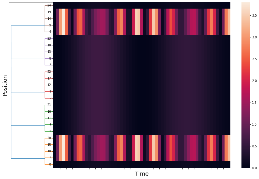
Figure 3: Numerical approximation for the interference pattern $\left|\Psi\left(x,t\right)\right|^{2}$ produced by a two slit experiment in the mid-range zone in dimension $1$. Take $p=5$, $L=2$, $a=0$ ($\left|a\right|_{5}=0$), $b=24$ ($\left|b\right|_{5}=1$). The mid-range zone is then $\left|x\right|_{5}\leq 1$ (the unit  ball $\mathbb{Z}_{5}$). The unit ball is approximated by the finite tree $G_{2}=\mathbb{Z}_{5}/5^{2}\mathbb{Z}_{5}$. The elements of this tree constitute the vertical scale. Horizontal scale corresponds to the time running on the interval $\left[0,3\right]$, with a step of $0.05$.

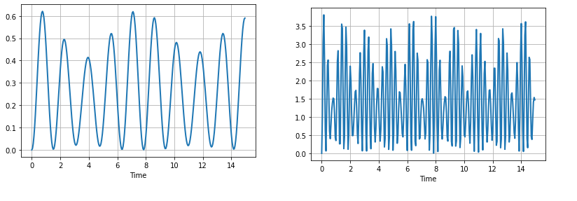
Figure 4: The left figure shows the interference pattern $\left|\Psi\left(6,t\right)\right|^{2}$, for $x=6$ ($\left|6\right|_{5}=1$) and $t$ running in the interval $\left[0,15\right]$. The right figure shows the interference pattern $\left|\Psi\left(5,t\right)\right|^{2}$, for $x=5$ ($\left|5\right|_{5}=5^{-1}$) and $t$ running in the interval $\left[0,15\right]$.

11 Appendix: basic facts on $p$-adic analysis

In this section, we fix the notation and collect some basic results on $p$-adic analysis that we will use throughout the article. For a detailed exposition on $p$-adic analysis the reader may consult [6], [75]-[81].

11.1 The field of $p$-adic numbers

In this article, $p$ denotes a prime number. The field of $p-$adic numbers $\mathbb{Q}_{p}$ is defined as the completion of the field of rational numbers $\mathbb{Q}$ with respect to the $p-$adic norm $|\cdot|_{p}$, which is defined as

$$|x|_{p}=\begin{cases}0&\text{if }x=0\\ p^{-\gamma}&\text{if }x=p^{\gamma}\dfrac{a}{b},\end{cases}$$

where $a$ and $b$ are integers coprime with $p$. The integer $\gamma=ord_{p}(x):=ord(x)$, with $ord(0):=+\infty$, is called the $p-$adic order of $x$. We extend the $p-$adic norm to $\mathbb{Q}_{p}^{N}$ by taking

$$||x||_{p}:=\max_{1\leq i\leq N}|x_{i}|_{p},\qquad\text{for }x=(x_{1},\dots,x_{N})\in\mathbb{Q}_{p}^{N}.$$

By defining $ord(x)=\min_{1\leq i\leq N}\{ord(x_{i})\}$, we have $||x||_{p}=p^{-ord(x)}$. The metric space $\left(\mathbb{Q}_{p}^{N},||\cdot||_{p}\right)$ is a complete ultrametric space. As a topological space $\mathbb{Q}_{p}$ is homeomorphic to a Cantor-like subset of the real line, see, e.g., [6], [75].

Any $p-$adic number $x\neq 0$ has a unique expansion of the form

$$x=p^{ord(x)}\sum_{j=0}^{\infty}x_{j}p^{j},$$

where $x_{j}\in\{0,1,2,\dots,p-1\}$ and $x_{0}\neq 0$.  In addition, any $x\in\mathbb{Q}_{p}^{N}\smallsetminus\left\{0\right\}$ can be represented uniquely as $x=p^{ord(x)}v$, where $\left\|v\right\|_{p}=1$.

11.2 Topology of $\mathbb{Q}_{p}^{N}$

For $r\in\mathbb{Z}$, denote by $B_{r}^{N}(a)=\{x\in\mathbb{Q}_{p}^{N};||x-a||_{p}\leq p^{r}\}$ the ball of radius $p^{r}$ with center at $a=(a_{1},\dots,a_{N})\in\mathbb{Q}_{p}^{N}$, and take $B_{r}^{N}(0):=B_{r}^{N}$. Note that $B_{r}^{N}(a)=B_{r}(a_{1})\times\cdots\times B_{r}(a_{N})$, where $B_{r}(a_{i}):=\{x\in\mathbb{Q}_{p};|x_{i}-a_{i}|_{p}\leq p^{r}\}$ is the one-dimensional ball of radius $p^{r}$ with center at $a_{i}\in\mathbb{Q}_{p}$. The ball $B_{0}^{N}$ equals the product of $N$ copies of $B_{0}=\mathbb{Z}_{p}$, the ring of $p-$adic integers. We also denote by $S_{r}^{N}(a)=\{x\in\mathbb{Q}_{p}^{N};||x-a||_{p}=p^{r}\}$ the sphere of radius $p^{r}$ with center at $a=(a_{1},\dots,a_{N})\in\mathbb{Q}_{p}^{N}$, and take $S_{r}^{N}(0):=S_{r}^{N}$. We notice that $S_{0}^{1}=\mathbb{Z}_{p}^{\times}$ (the group of units of $\mathbb{Z}_{p}$), but $\left(\mathbb{Z}_{p}^{\times}\right)^{N}\subsetneq S_{0}^{N}$. The balls and spheres are both open and closed subsets in $\mathbb{Q}_{p}^{N}$. In addition, two balls in $\mathbb{Q}_{p}^{N}$ are either disjoint or one is contained in the other.

As a topological space $\left(\mathbb{Q}_{p}^{N},||\cdot||_{p}\right)$ is totally disconnected, i.e., the only connected  subsets of $\mathbb{Q}_{p}^{N}$ are the empty set and the points. A subset of $\mathbb{Q}_{p}^{N}$ is compact if and only if it is closed and bounded in $\mathbb{Q}_{p}^{N}$, see, e.g., [6, Section 1.3], or [75, Section 1.8]. The balls and spheres are compact subsets. Thus $\left(\mathbb{Q}_{p}^{N},||\cdot||_{p}\right)$ is a locally compact topological space.

11.3 The Haar measure

Since $(\mathbb{Q}_{p}^{N},+)$ is a locally compact topological group, there exists a Haar measure $d^{N}x$, which is invariant under translations, i.e., $d^{N}(x+a)=d^{N}x$, [83]. If we normalize this measure by the condition $\int_{\mathbb{Z}_{p}^{N}}dx=1$, then $d^{N}x$ is unique.

Notation 1

We will use $\Omega\left(p^{-r}||x-a||_{p}\right)$ to denote the characteristic function of the ball $B_{r}^{N}(a)=a+p^{-r}\mathbb{Z}_{p}^{N}$, where

$$\mathbb{Z}_{p}^{N}=\left\{x\in\mathbb{Q}_{p}^{N};\left\|x\right\|_{p}\leq 1\right\}$$

is the $N$-dimensional unit ball. For more general sets, we will use the notation $1_{A}$ for the characteristic function of set $A$.

11.4 The Bruhat-Schwartz space

A complex-valued function $\varphi$ defined on $\mathbb{Q}_{p}^{N}$ is called locally constant if for any $x\in\mathbb{Q}_{p}^{N}$ there exist an integer $l(x)\in\mathbb{Z}$ such that

$$\varphi(x+x^{\prime})=\varphi(x)\text{ for any }x^{\prime}\in B_{l(x)}^{N}.$$ (11.1)

A function $\varphi:\mathbb{Q}_{p}^{N}\rightarrow\mathbb{C}$ is called a Bruhat-Schwartz function (or a test function) if it is locally constant with compact support. Any test function can be represented as a linear combination, with complex coefficients, of characteristic functions of balls. The $\mathbb{C}$-vector space of Bruhat-Schwartz functions is denoted by $\mathcal{D}(\mathbb{Q}_{p}^{N})$. For $\varphi\in\mathcal{D}(\mathbb{Q}_{p}^{N})$, the largest number $l=l(\varphi)$ satisfying (11.1) is called the exponent of local constancy (or the parameter of constancy) of $\varphi$.

We denote by $\mathcal{D}_{m}^{l}(\mathbb{Q}_{p}^{N})$ the finite-dimensional space of test functions from $\mathcal{D}(\mathbb{Q}_{p}^{N})$ having supports in the ball $B_{m}^{N}$ and with parameters  of constancy $\geq l$. We now define a topology on $\mathcal{D}(\mathbb{Q}_{p}^{N})$ as follows. We say that a sequence $\left\{\varphi_{j}\right\}_{j\in\mathbb{N}}$ of functions in $\mathcal{D}(\mathbb{Q}_{p}^{N})$ converges to zero, if the two following conditions hold true:

(1) there are two fixed integers $k_{0}$ and $m_{0}$ such that  each $\varphi_{j}\in$ $\mathcal{D}_{m_{0}}^{k_{0}}(\mathbb{Q}_{p}^{N})$;

(2) $\varphi_{j}\rightarrow 0$ uniformly.

$\mathcal{D}(\mathbb{Q}_{p}^{N})$ endowed with the above topology becomes a topological vector space.

11.5 $L^{\rho}$ spaces

Given $\rho\in[0,\infty)$, we denote by$L^{\rho}\left(\mathbb{Q}_{p}^{N}\right):=L^{\rho}\left(\mathbb{Q}_{p}^{N},d^{N}x\right),$ the $\mathbb{C}-$vector space of all the complex valued functions $g$ satisfying

$$\left\|g\right\|_{\rho}=\left(\text{ }\mathop{\displaystyle\int}\limits_{\mathbb{Q}_{p}^{N}}\left|g\left(x\right)\right|^{\rho}d^{N}x\right)^{\frac{1}{\rho}}<\infty,$$

where $d^{N}x$ is the normalized Haar measure on $\left(\mathbb{Q}_{p}^{N},+\right)$.

If $U$ is an open subset of $\mathbb{Q}_{p}^{N}$, $\mathcal{D}(U)$ denotes the $\mathbb{C}$-vector space of test functions with supports contained in $U$, then $\mathcal{D}(U)$ is dense in

$$L^{\rho}\left(U\right)=\left\{\varphi:U\rightarrow\mathbb{C};\left\|\varphi\right\|_{\rho}=\left\{\mathop{\displaystyle\int}\limits_{U}\left|\varphi\left(x\right)\right|^{\rho}d^{N}x\right\}^{\frac{1}{\rho}}<\infty\right\},$$

for $1\leq\rho<\infty$, see, e.g., [75, Section 4.3]. We denote by $L_{\mathbb{R}}^{\rho}\left(U\right)$ the real counterpart of $L^{\rho}\left(U\right)$.

11.6 The Fourier transform

Set $\chi_{p}(y)=\exp(2\pi i\{y\}_{p})$ for $y\in\mathbb{Q}_{p}$, and $\xi\cdot x:=\sum_{j=1}^{N}\xi_{j}x_{j}$, for $\xi=(\xi_{1},\dots,\xi_{N})$, $x=(x_{1},\dots,x_{N})\allowbreak\in\mathbb{Q}_{p}^{N}$, as before. The Fourier transform of $\varphi\in\mathcal{D}(\mathbb{Q}_{p}^{N})$ is defined as

$$\mathcal{F}\varphi(\xi)=\mathop{\displaystyle\int}\limits_{\mathbb{Q}_{p}^{N}}\chi_{p}(\xi\cdot x)\varphi(x)d^{N}x\quad\text{for }\xi\in\mathbb{Q}_{p}^{N},$$

where $d^{N}x$ is the normalized Haar measure on $\mathbb{Q}_{p}^{N}$. The Fourier transform is a linear isomorphism from $\mathcal{D}(\mathbb{Q}_{p}^{N})$ onto itself satisfying

$$(\mathcal{F}(\mathcal{F}\varphi))(\xi)=\varphi(-\xi),$$ (11.2)

see, e.g., [75, Section 4.8]. We also use the notation $\mathcal{F}_{x\rightarrow\kappa}\varphi$ and $\widehat{\varphi}$ for the Fourier transform of $\varphi$.

The Fourier transform extends to $L^{2}$. If $f\in L^{2}\left(\mathbb{Q}_{p}^{N}\right)$, its Fourier transform is defined as

$$(\mathcal{F}f)(\xi)=\lim_{k\rightarrow\infty}\mathop{\displaystyle\int}\limits_{||x||_{p}\leq p^{k}}\chi_{p}(\xi\cdot x)f(x)d^{N}x,\quad\text{for }\xi\in\mathbb{Q}_{p}^{N},$$

where the limit is taken in $L^{2}\left(\mathbb{Q}_{p}^{N}\right)$. We recall that the Fourier transform is unitary on $L^{2}\left(\mathbb{Q}_{p}^{N}\right)$, i.e. $||f||_{2}=||\mathcal{F}f||_{2}$ for $f\in L^{2}\left(\mathbb{Q}_{p}^{N}\right)$ and that (11.2) is also valid in $L^{2}\left(\mathbb{Q}_{p}^{N}\right)$, see, e.g., [81, Chapter III, Section 2].

11.7 Distributions

The $\mathbb{C}$-vector space $\mathcal{D}^{\prime}\left(\mathbb{Q}_{p}^{N}\right)$ of all continuous linear functionals on $\mathcal{D}(\mathbb{Q}_{p}^{N})$ is called the Bruhat-Schwartz space of distributions. Every linear functional on $\mathcal{D}(\mathbb{Q}_{p}^{N})$ is continuous, i.e. $\mathcal{D}^{\prime}\left(\mathbb{Q}_{p}^{N}\right)$ agrees with the algebraic dual of $\mathcal{D}(\mathbb{Q}_{p}^{N})$, see, e.g., [6, Chapter 1, VI.3, Lemma].

We endow $\mathcal{D}^{\prime}\left(\mathbb{Q}_{p}^{N}\right)$ with the weak topology, i.e. a sequence $\left\{T_{j}\right\}_{j\in\mathbb{N}}$ in $\mathcal{D}^{\prime}\left(\mathbb{Q}_{p}^{N}\right)$ converges to $T$ if $\lim_{j\rightarrow\infty}T_{j}\left(\varphi\right)=T\left(\varphi\right)$ for any $\varphi\in\mathcal{D}(\mathbb{Q}_{p}^{N})$. The map

$$\begin{array}[]{lll}\mathcal{D}^{\prime}\left(\mathbb{Q}_{p}^{N}\right)\times\mathcal{D}(\mathbb{Q}_{p}^{N})&\rightarrow&\mathbb{C}\\ \left(T,\varphi\right)&\rightarrow&T\left(\varphi\right)\end{array}$$

is a bilinear form which is continuous in $T$ and $\varphi$ separately. We call this map the pairing between $\mathcal{D}^{\prime}\left(\mathbb{Q}_{p}^{N}\right)$ and $\mathcal{D}(\mathbb{Q}_{p}^{N})$. From now on we will use $\left(T,\varphi\right)$ instead of $T\left(\varphi\right)$.

Every $f$ in $L_{loc}^{1}$ defines a distribution $f\in\mathcal{D}^{\prime}\left(\mathbb{Q}_{p}^{N}\right)$ by the formula

$$\left(f,\varphi\right)=\mathop{\displaystyle\int}\limits_{\mathbb{Q}_{p}^{N}}f\left(x\right)\varphi\left(x\right)d^{N}x.$$

11.8 The Fourier transform of a distribution

The Fourier transform $\mathcal{F}\left[T\right]$ of a distribution $T\in\mathcal{D}^{\prime}\left(\mathbb{Q}_{p}^{N}\right)$ is defined by

$$\left(\mathcal{F}\left[T\right],\varphi\right)=\left(T,\mathcal{F}\left[\varphi\right]\right)\text{ for all }\varphi\in\mathcal{D}\left(\mathbb{Q}_{p}^{N}\right)\text{.}$$

The Fourier transform $T\rightarrow\mathcal{F}\left[T\right]$ is a linear and continuous isomorphism from $\mathcal{D}^{\prime}\left(\mathbb{Q}_{p}^{N}\right)$ onto $\mathcal{D}^{\prime}\left(\mathbb{Q}_{p}^{N}\right)$. Furthermore, $T=\mathcal{F}\left[\mathcal{F}\left[T\right]\left(-\xi\right)\right]$.

Let $T\in\mathcal{D}^{\prime}\left(\mathbb{Q}_{p}^{n}\right)$ be a distribution. Then supp$T\subset B_{L}^{N}$ if and only if $\mathcal{F}\left[T\right]$ is a locally constant function, and the exponent of local constancy of $\mathcal{F}\left[T\right]$ is $\geq-L$. In addition

$$\mathcal{F}\left[T\right]\left(\xi\right)=\left(T\left(y\right),\Omega\left(p^{-L}\left\|y\right\|_{p}\right)\chi_{p}\left(\xi\cdot y\right)\right),$$

see, e.g., [75, Section 4.9].

11.9 The direct product of distributions

Given $F\in\mathcal{D}^{\prime}\left(\mathbb{Q}_{p}^{N}\right)$ and $G\in\mathcal{D}^{\prime}\left(\mathbb{Q}_{p}^{M}\right)$, their direct product $F\times G$ is defined by the formula

$$\left(F\left(x\right)\times G\left(y\right),\varphi\left(x,y\right)\right)=\left(F\left(x\right),\left(G\left(y\right),\varphi\left(x,y\right)\right)\right)\text{ for }\varphi\left(x,y\right)\in\mathcal{D}\left(\mathbb{Q}_{p}^{N+M}\right).$$

The direct product is commutative: $F\times G=G\times F$. In addition the direct product is continuous with respect to the joint factors.

11.10 The convolution of distributions

Given $F,G\in\mathcal{D}^{\prime}\left(\mathbb{Q}_{p}^{N}\right)$, their convolution $F\ast G$ is defined by

$$\left(F\ast G,\varphi\right)=\lim_{k\rightarrow\infty}\left(F\left(y\right)\times G\left(x\right),\Omega\left(p^{-k}\left\|y\right\|_{p}\right)\varphi\left(x+y\right)\right)$$

if the limit exists for all $\varphi\in\mathcal{D}\left(\mathbb{Q}_{p}^{N}\right)$. We recall that if $F\ast G$ exists, then $G\ast F$ exists and $F\ast G=G\ast F$, see, e.g., [6, Section 7.1]. If $F,G\in\mathcal{D}^{\prime}\left(\mathbb{Q}_{p}^{N}\right)$ and supp$G\subset B_{L}^{n}$, then the convolution $F\ast G$ exists, and it is given by the formula

$$\left(F\ast G,\varphi\right)=\left(F\left(y\right)\times G\left(x\right),\Omega\left(p^{-L}\left\|y\right\|_{p}\right)\varphi\left(x+y\right)\right)\text{ for }\varphi\in\mathcal{D}\left(\mathbb{Q}_{p}^{N}\right).$$

In the case in which $G=\psi\in\mathcal{D}\left(\mathbb{Q}_{p}^{n}\right)$, $F\ast\psi$ is a locally constant function given by

$$\left(F\ast\psi\right)\left(y\right)=\left(F\left(x\right),\psi\left(y-x\right)\right),$$

see, e.g., [6, Section 7.1].

11.11 The multiplication of distributions

Set $\delta_{k}\left(x\right):=p^{Nk}\Omega\left(p^{k}\left\|x\right\|_{p}\right)$ for $k\in\mathbb{N}$. Given $F,G\in\mathcal{D}^{\prime}\left(\mathbb{Q}_{p}^{N}\right)$, their product $F\cdot G$ is defined by

$$\left(F\cdot G,\varphi\right)=\lim_{k\rightarrow\infty}\left(G,\left(F\ast\delta_{k}\right)\varphi\right)$$

if the limit exists for all $\varphi\in\mathcal{D}\left(\mathbb{Q}_{p}^{N}\right)$. If the product $F\cdot G$ exists then the product $G\cdot F$ exists and they are equal.

We recall that  the existence of the product $F\cdot G$ is equivalent  to the existence of $\mathcal{F}\left[F\right]\ast\mathcal{F}\left[G\right]$. In addition, $\mathcal{F}\left[F\cdot G\right]=\mathcal{F}\left[F\right]\ast\mathcal{F}\left[G\right]$ and $\mathcal{F}\left[F\ast G\right]=\mathcal{F}\left[F\right]\cdot\mathcal{F}\left[G\right]$, see, e.g., [6, Section 7.5].

Acknowledgement 1

The author whishes to thank B. A. Zambrano-Luna for his kind assistance in the elaboration of Figures 3-4.

References

- [1] Dirac P. A. M.,The principles of quantum mechanics. First edition 1930. Fourth Edition, Oxford University Press. 1958.
- [2] von Neumann John, Mathematical foundations of quantum Mechanics. First Edition 1932. Princeton University Press, Princeton, NJ, 2018.
- [3] Berezin F. A., Shubin M. A., The Schrödinger equation. Math. Appl. (Soviet Ser.), 66 Kluwer Academic Publishers Group, Dordrecht, 1991.
- [4] Takhtajan Leon A., Quantum mechanics for mathematicians, Graduate Studies in Mathematics, vol. 95, American Mathematical Society, 2008.
- [5] Komech A., Quantum Mechanics: Genesis and Achievements, Springer, Dordrecht, 2013.
- [6] Vladimirov V. S., Volovich I. V., Zelenov E. I., -Adic analysis and mathematical physics. World Scientific, 1994.
- [7] Kochubei A.N., Pseudo-differential equations and stochastics over non-Archimedean fields. Marcel Dekker, New York, 2001.
- [8] Zúñiga-Galindo W. A., Pseudodifferential equations over non-Archimedean spaces. Lecture Notes in Mathematics, 2174. Springer, Cham, 2016.
- [9] Bendikov A., Grigor’yan A., Pittet C. and Woess W., Isotropic Markov semigroups on ultra-metric spaces. Russian Math. Surveys 69 (2014), 589–680.
- [10] Aharonov Y., Cohen E., Colombo F., Landsberger T., Sabadini I., Struppa D., and Tollaksen J., Finally making sense of the double-slit experiment. Proc. Natl. Acad. Sci. U. S. A. 114, 6480 (2017).
- [11] Bronstein M., Republication of: Quantum theory of weak gravitational fields. Gen Relativ Gravit 44, 267–283 (2012).
- [12] Volovich I. V., Number theory as the ultimate physical theory. -Adic Numbers Ultrametric Anal. Appl. 2 (2010), no. 1, 77–87.
- [13] Rovelli C. and Vidotto F., Covariant Loop Quantum Gravity: An Elementary Introduction to Quantum Gravity and Spinfoam Theory. Cambridge University Press, 2015.
- [14] Beltrametti E. G., Cassinelli G., Quantum mechanics and p-adic numbers. Found. Phys. 2 (1972), 1–7.
- [15] Vladimirov V. S., Volovich I. V., p-adic quantum mechanics, Soviet Phys. Dokl. 33 (1988), no. 9, 669–670.
- [16] Vladimirov V. S., Volovich, I. V., A vacuum state in p-adic quantum mechanics. Phys. Lett. B 217 (1989), no. 4, 411–415.
- [17] Vladimirov V. S., Volovich I. V., -adic quantum mechanics. Comm. Math. Phys. 123 (1989), no. 4, 659–676.
- [18] Meurice, Yannick, Quantum mechanics with p-adic numbers. Internat. J. Modern Phys. A 4 (1989), no. 19, 5133–5147.
- [19] Zelenov, E. I., p-adic quantum mechanics for . Theoret. and Math. Phys. 80 (1989), no. 2, 848–856.
- [20] Ruelle Ph., Thiran E., Verstegen D., Weyers J., Quantum mechanics on -adic fields. J. Math. Phys. 30 (1989), no. 12, 2854–2874.
- [21] Vladimirov V. S., Volovich I. V., Zelenov E. I., Spectral theory in -adic quantum mechanics and representation theory. Soviet Math. Dokl. 41 (1990), no. 1, 40–44.
- [22] Ismagilov R. S., On the spectrum of a selfadjoint operator in L2(K), where K is a local field; an analogue of the Feynman-Kac formula. Theoret. and Math. Phys. 89 (1991), no.1, 1024–1028.
- [23] Meurice Yannick, A discretization of p-adic quantum mechanics. Comm. Math. Phys. 135 (1991), no. 2, 303–312.
- [24] Khrennikov A. Yu, -adic quantum mechanics with -adic valued functions. J. Math. Phys. 32 (1991), no. 4, 932–937.
- [25] Zelenov E. I., -adic quantum mechanics and coherent states. Theoret. and Math. Phys. 86 (1991), no. 2, 143–151.
- [26] Zelenov E. I., -adic quantum mechanics and coherent states. II. Oscillator eigenfunctions. Theoret. and Math. Phys. 86 (1991), no. 3, 258–265.
- [27] Kochubei Anatoly N., A Schrödinger-type equation over the field of -adic numbers. J. Math. Phys. 34 (1993), no. 8, 3420–3428.
- [28] Cianci Roberto, Khrennikov Andrei, -adic numbers and renormalization of eigenfunctions in quantum mechanics. Phys. Lett. B 328 (1994), no. 1-2, 109–112.
- [29] Blair Alan D., Adèlic path space integrals. Rev. Math. Phys. 7 (1995), no. 1, 21–49.
- [30] Kochubei Anatoly N., -Adic commutation relations. J. Phys. A 29 (1996), no. 19, 6375–6378.
- [31] Varadarajan V. S., Path integrals for a class of p-adic Schrödinger equations. Lett. Math. Phys. 39 (1997), no. 2, 97–106.
- [32] Khrennikov A., Non-Kolmogorov probabilistic models with -adic probabilities and foundations of quantum mechanics. Progr. Probab., 42. Birkhäuser Boston, Inc., Boston, MA, 1998, 275–303.
- [33] Albeverio S., Cianci R., De Grande-De Kimpe N., Khrennikov A., -adic probability and an interpretation of negative probabilities in quantum mechanics. Russ. J. Math. Phys. 6 (1999), no. 1, 1–19.
- [34] Dimitrijević D., Djordjević G. S., Dragovich B., On Schrödinger-type equation on p-adic spaces. Bulgar. J. Phys. 27 (2000), no. 3, 50–53.
- [35] Dragovich B., -adic and adelic quantum mechanics. Proc. Steklov Inst. Math. (2004), no. 2, 64–77.
- [36] Vourdas A., Quantum mechanics on -adic numbers. J. Phys. A 41 (2008), no. 45, 455303, 20 pp.
- [37] Dragovich B., Khrennikov A. Yu., Kozyrev S. V., Volovich, I. V., On -adic mathematical physics. -Adic Numbers Ultrametric Anal. Appl. 1 (2009), no. 1, 1–17.
- [38] Zelenov E. I., -adic model of quantum mechanics and quantum channels. Proc. Steklov Inst. Math. 285 (2014), no. 1, 132–144.
- [39] Anashin V., Free Choice in Quantum Theory: A -adic View. Entropy 2023; 25(5):830. https://doi.org/10.3390/e25050830.
- [40] Aniello Paolo, Mancini Stefano, Parisi Vincenzo, Trace class operators and states in -adic quantum mechanics. J. Math. Phys. 64 (2023), no. 5, Paper No. 053506, 45 pp.
- [41] Aref’eva I. Ya., Volovich I. V., Quantum group particles and non-Archimedean geometry. Phys. Lett. B 268 (1991), no. 2, 179–187.
- [42] Baxter Rodney J., Exactly solved models in statistical mechanics. Academic Press, Inc., London, 1982.
- [43] Biedenharn L. C., The quantum group and a -analogue of the boson operators. J. Phys. A 22 (1989), no. 18, L873–L878.
- [44] Ernst Thomas, A comprehensive treatment of -calculus. Birkhäuser/Springer Basel AG, Basel, 2012.
- [45] Ayşe Erzan, Jean-Pierre Eckmann, -Analysis of fractal sets. Phys. Rev. Lett. 78 (1997), no. 17, 3245–3248.
- [46] Finkelstein R. J., Quantum groups and field theory, Modern Phys. Lett. A 15 (2000), no. 28, 1709–1715.
- [47] Finkelstein R. J., Observable properties of -deformed physical systems. Lett. Math. Phys. 49 (1999), no. 2, 105–114.
- [48] Kac Victor, Pokman Cheung, Quantum calculus. Universitext. Springer-Verlag, New York, 2002.
- [49] Klimyk Anatoli, Schmüdgen Konrad, Quantum groups and their representations. Texts and Monographs in Physics. Springer-Verlag, Berlin, 1997.
- [50] Lavagno A., Basic-deformed quantum mechanics. Rep. Math. Phys. 64 (2009), no. 1-2, 79–91.
- [51] Lavagno A., Deformed quantum mechanics and -Hermitian operators. J. Phys. A 41 (2008), no. 24, 244014, 9 pp.
- [52] Lavagno A., A. M. Scarfone, P. Narayana Swamy, Basic-deformed thermostatistics. J. Phys. A 40 (2007), no. 30, 8635–8654.
- [53] Macfarlane A. J. , On -analogues of the quantum harmonic oscillator and the quantum group . J. Phys. A 22 (1989), no. 21, 4581–4588.
- [54] Manin Yuri I., Quantum groups and noncommutative geometry. Second edition. CRM Short Courses. Springer, Cham, 2018.
- [55] Wess Julius, Zumino Bruno, Covariant differential calculus on the quantum hyperplane. Nuclear Phys. B Proc. Suppl. 18B (1990), 302–312 (1991).
- [56] Zhang Jian-zu, Spectrum of -deformed Schrödinger equation. Phys. Lett. B 477 (2000), no. 1-3, 361–366.
- [57] Zhang Jian-zu, A -deformed uncertainty relation. Phys. Lett. A 262 (1999), no. 2-3, 125–130.
- [58] Zhang Jian-zu, A -deformed quantum mechanics. Phys. Lett. B 440 (1998), no. 1-2, 66–68.
- [59] Zúñiga-Galindo W. A., Non-Archimedean quantum mechanics via quantum groups. Nuclear Phys. B985 (2022), Paper No. 116021, 21 pp.
- [60] Schwinger Julian, Unitary operator bases. Proc. Nat. Acad. Sci. U.S.A.46 (1960), 570–579.
- [61] Schwinger Julian, The special canonical group. Proc. Nat. Acad. Sci. U.S.A. 46 (1960), 1401–1415.
- [62] Weyl H., The theory of groups and quantum mechanics. Dutton, NY, 1932
- [63] Digernes Trond, Varadarajan V. S., Varadhan S. R. S., Finite approximations to quantum systems. Rev. Math. Phys.6(1994), no.4, 621–648.
- [64] Varadarajan V.S., Non-Archimedean models for space-time. Mod. Phys. Lett. A. 2001. V. 16. P. 387–395.
- [65] V. S. Varadarajan, Arithmetic Quantum Physics: Why, What, and Whither. Trudy, Mat. Inst. Steklova, 2004, Volume 245, 273–280.
- [66] Vourdas, A., Quantum systems with finite Hilbert space. Rep. Progr. Phys. 67 (2004), no.3, 267–320.
- [67] Bakken E. M., Digernes T., Finite approximations of physical models over local fields. -Adic Numbers Ultrametric Anal. Appl. 7 (2015), no. 4, 245–258.
- [68] Digernes Trond, A review of finite approximations, Archimedean and non-Archimedean. p-Adic Numbers Ultrametric Anal. Appl. 10 (2018), no. 4, 253–266.
- [69] Vourdas Apostolos, Finite and profinite quantum systems. Quantum Sci. Technol. Springer, Cham, 2017.
- [70] Zúñiga-Galindo W. A. and others, -Adic statistical field theory and convolutional deep Boltzmann machines, Progress of Theoretical and Experimental Physics, Volume 2023, Issue 6, June 2023, 063A01, https://doi.org/10.1093/ptep/ptad061.
- [71] Zúñiga-Galindo W.A., -adic statistical field theory and deep belief networks, Physica A: Statistical Mechanics and its Applications, 612 (2023), Paper No. 128492, 23 pp.
- [72] Taira Kazuaki, Boundary value problems and Markov processes. Functional analysis methods for Markov processes. Third edition.Lecture Notes in Math., 1499. Springer, Cham, 2020.
- [73] Chistyakov D. V. Fractal geometry of images of continuous embeddings of p-adic numbers and solenoids into Euclidean spaces,Theoret. and Math. Phys.109 (1996), no.3, 1495–1507.
- [74] Zee A., Quantum field theory in a nutshell. Second edition Princeton University Press, Princeton, NJ, 2010.
- [75] Albeverio S., Khrennikov A. Yu., Shelkovich V. M., Theory of -adic distributions: linear and nonlinear models. London Mathematical Society Lecture Note Series, 370. Cambridge University Press, 2010.
- [76] Khrennikov Andrei, Kozyrev Sergei, Zúñiga-Galindo W. A., Ultrametric Equations and its Applications. Encyclopedia of Mathematics and its Applications (168), Cambridge University Press, 2018.
- [77] Evans Steven N., Local field Gaussian measures. Seminar on Stochastic Processes, 1988, 121–160. Progr. Probab., 17 Birkhäuser Boston, Inc., Boston, MA, 1989.
- [78] McClendon M. and Rabitz H., Numerical simulations in stochastic mechanics. Phys. Rev. A, 37 (1988), 3479-3492.
- [79] Webb G.F., Event Based Interpretation of Schrödinger’s Equation for the Two-slit Experiment. Int J Theor Phys 50, 3571–3601 (2011).
- [80] Webb Glenn, The Schrödinger equation and the two-slit experiment of quantum mechanics. Discrete and Continuous Dynamical Systems - S. doi: 10.3934/dcdss.2023001.
- [81] M. H. Taibleson, Fourier analysis on local fields. Princeton University Press, 1975.
- [82] Bendikov Alexander, Grigor’yan Alexander, Molchanov Stanislav, Hierarchical Schrödinger type operators: the case of locally bounded potentials. Operator theory and harmonic analysis—OTHA 2020. Part II. Probability-analytical models, methods and applications, 43–89. Springer Proc. Math. Stat., 358 Springer, Cham, 2021.
- [83] Halmos P., Measure Theory. D. Van Nostrand Company Inc., New York, 1950.