Quantum Algorithms for the computation of quantum thermal averages at work

Abstract

Recently, a variety of quantum algorithms have been devised to estimate thermal averages on a genuine quantum processor. In this paper, we consider the practical implementation of the so-called Quantum-Quantum Metropolis algorithm. As a testbed for this purpose, we simulate a basic system of three frustrated quantum spins and discuss its systematics, also in comparison with the Quantum Metropolis Sampling algorithm.

I Introduction

The advent of quantum computation is expected to lead to breakthroughs in various fields of computational science [1, 2, 3]. In fact, it may disclose novel pathways to the solution of notable unsolved questions lying at the basis of classically intractable problems, from quantum chemistry, to condensed-matter and high-energy physics [4, 5]. One of such examples deals with the physics of fundamental interactions, in particular when considering the strongly coupled regime, which is not treatable by perturbative analytical tools. Classical computational schemes, based on a discretized path integral formulation, are indeed known to face hard and yet unsolved difficulties. This happens, for instance, when considering real-time processes and non-equilibrium physics, or even in the equilibrium case when the path-integral measure is not positive defined (as it happens at finite baryon density), a fact which prevents the application of classical Monte Carlo algorithms. Such an algorithmic obstruction is, for example, the main reason for our incomplete knowledge of the QCD phase diagram and of the physics of strongly interacting matter at finite density, which is required for the investigation of compact astrophysical objects [6, 7].

In the case of equilibrium physics, one needs to devise quantum algorithms capable to efficiently explore the Gibbs ensemble of the target quantum system. At present, the availability of quantum resources adequate for the numerical investigation of systems of direct physical interest, such as QCD, is still far from being achieved. Nevertheless, a variety of candidate quantum algorithms have been already proposed, either by directly computing observables on the (mixed) thermal state [8, 9, 10, 11, 12], or by preparing an ensemble of pure states, sampled with the proper thermal distribution [13, 14, 15, 16, 17, 18, 19, 20, 21, 22, 23, 24, 25]. At the present stage, it is thus important to investigate how the practical implementation of such algorithms works in simplified models, in order to better understand their systematics and pave the way to future and more realistic applications.

In Ref. [26], some of the present authors have already focused on the so-called Quantum Metropolis Sampling (QMS) algorithm [13], applied to a simple frustrated system made up of three quantum spins, which presents a sign problem when formulated in the path-integral approach. The QMS algorithm is based on a quantum Metropolis step, by which one can implement a quantum Markov chain across the Hamiltonian eigenstates of the system, which is capable of correctly sampling, after a proper thermalization time, the quantum eigenstates with the desired ensemble probability. In this paper, we also consider the alternative Quantum-Quantum Metropolis Algorithm (Q²MA) [14], which is based on a quite different strategy. In a few words, the idea is to search for a pure quantum state, the so-called coherent encoding of the thermal state (CETS), with the property that a measurement of the Hamiltonian on such state returns a given eigenstate with the correct Gibbs distribution. The search follows a Grover-like quantum approach, hence the double “Quantum” in the name of the algorithm, which therefore, at least in principle, promises a more effective quantum advantage.

A fundamental ingredient for both approaches is the Quantum Phase Estimation (QPE) algorithm [27, 28, 29, 30], which allows to estimate the energy eigenvalues once the Hamiltonian has been properly encoded in the quantum computer. However, the overall strategy used in the two methods is quite different: in the QMS algorithm the distribution is sampled via the Metropolis step, while in the Q²MA algorithm it is encoded in the superposition amplitudes of a pure state, which contains the information about the finite-temperature density matrix of the system, once the auxiliary registers are traced out.

We are not aware of practical implementations and benchmarks of the Q²MA algorithm in concrete examples, and the main purpose of the present study is to fill this gap, by considering the same target system of Ref. [26]. As we will discuss in more details later on, there are some aspects of the algorithm which make its practical implementation nontrivial.

A different issue regards the numerical efficiency, measured in terms of the number of quantum gates needed to reach a given uncertainty on the final determination of the quantum thermal averages, for which we present a preliminary comparison between the two algorithms. In carrying out such an analysis, particular attention is taken towards both statistical and systematic contributions to the final error budget.

The paper is organized as follows. In Sec. II, we first review the basic features of the QMS and the Q²MA algorithms, and then comment on the possible sources of systematical errors. In Sec. III, we introduce the specific quantum spin system tested here and all the metrics used to benchmark the systematical errors. In Sec. IV, we present the results of our investigation, first assuming an exact encoding of the energy levels and then relaxing such constraint. Finally, our conclusions are drawn in Sec. V.

II Algorithms

The main focus of the present study is on the Q²MA algorithm, since a practical implementation of the QMS algorithm has been already presented and discussed in Ref. [26]. However, we find it useful to give a brief overview of both algorithms, in order to clarify their computational requirements and to better identify the possible sources of systematical errors in both cases.

II.1 Quantum Metropolis Sampling

The QMS algorithm follows quite closely the scheme of the classical Metropolis algorithm (see Refs. [13, 26] for further details): a Markov chain is built in such a way that, at each step, one gets an eigenstate $|\varphi_{k}\rangle$ of the Hamiltonian of the system under study, with eigenvalue $E_{k}$. This is selected with a probability given (asymptotically after thermalization) by its Boltzmann weight $e^{-\beta E_{k}}/Z(\beta)$, where $\beta=1/(k_{B}T)$ is the inverse temperature and $Z(\beta)$ is the partition function.

Four registers are required: a register encoding the state of the system (denoted by the subscript $1$), two energy registers encoding the energies before (denoted by $2$) and after (denoted by $3$) the Metropolis step, if accepted, and finally a single-qubit acceptance register (denoted by $4$). The layout of the quantum state needed by the QMS algorithm is thus the following:

$$\ket{\text{acc}}_{4}\ket{E_{\text{new}}}_{3}\ket{E_{\text{old}}}_{2}\ket{\mathrm{state}}_{1}\ .$$ (1)

The first step of the Markov chain is the initialization of the system state in register 1 to an arbitrary eigenstate of the Hamiltonian (and of register 2 to the corresponding eigenvalue). If the quantum state of the QMS algorithm has been prepared in the initial state $\ket{0}_{4}\ket{0}_{3}\ket{0}_{2}\ket{0}_{1}$, this can be realized by using a QPE between registers $1$ and $2$, followed by a measure of register $2$:

$$\ket{0}_{2}\ket{0}_{1} \xrightarrow{\mathrm{QPE}_{1,2}}\sum_{k^{\prime}}\alpha_{k^{\prime}}\ket{E_{k^{\prime}}}_{2}\ket{\varphi_{k^{\prime}}}_{1}$$ (2)

$$\xrightarrow{\mathrm{Meas}_{2}}\ket{E_{k}}_{2}\ket{\varphi_{k}}_{1}\ .$$

Registers $3$ and $4$ stay unmodified in this initial step.

A single step of the Markov chain involves an appropriate generalization of the Metropolis accept/reject algorithm [31] to the quantum case. In order to update the state, we apply to register 1 a unitary operator $C$ randomly selected from a set $\mathcal{C}$; this set has to be large enough to ensure mixing between all eigenstates (ergodicity) and that if $A\in\mathcal{C}$ then also $A^{-1}\in\mathcal{C}$ (reversibility). Apart from these general requirements, there is still much freedom in the choice of the operators entering the set $\mathcal{C}$, freedom that can eventually be used to optimize the algorithm. Thus

$$\ket{\varphi_{k}}_{1}\xrightarrow{C\in\mathcal{C}}\sum\limits_{p}x_{k,p}^{(C)}\ket{\varphi_{p}}_{1}\ .$$ (3)

At this point, we perform a second QPE between the register of the system (labeled as $1$) and the new energy register (labeled as $3$):

$$\sum\limits_{p}x_{k,p}^{(C)}\ket{0}_{4}\ket{0}_{3}\ket{E_{k}}_{2}\ket{\varphi_{p}}_{1}$$ (4)

$$\xrightarrow{\mathrm{QPE}_{1,3}}\sum\limits_{p}x_{k,p}^{(C)}\ket{0}_{4}\ket{E_{p}}_{3}\ket{E_{k}}_{2}\ket{\varphi_{p}}_{1}\ .$$

To introduce the information about the Boltzmann weights, one applies an oracle operator $G$ which reads out the difference between the two energy registers and acts on the acceptance qubit as follows:

$$\ket{0}_{4}\ket{E_{p}}_{3}\ket{E_{k}}_{2}\ket{\psi_{p}}_{1}\xrightarrow{G}$$ (5)

$$\left(\sqrt{f_{p,k}}\ket{1}_{4}+\sqrt{1-f_{p,k}}\ket{0}_{4}\right)\otimes\ket{E_{p}}_{3}\ket{E_{k}}_{2}\ket{\psi_{p}}_{1}\,,$$

where

$$f_{p,k}=\min\left(1,e^{-\beta(E_{p}-E_{k})}\right),$$ (6)

is the usual Metropolis acceptance probability. At this stage, one performs a measurement in the acceptance register 4, which can only take two outcomes: the value $1$ with probability $\sum_{p}|x_{k,p}^{(C)}|^{2}f_{p,k}$ and the value $0$ with the complementary probability. The first case corresponds to the “accepted” move, and the resulting state will be a superposition of eigenstates of the form

$$\sum\limits_{p}x_{k,p}^{(C)}\sqrt{f_{p,k}}\ket{1}_{4}\ket{E_{p}}_{3}\ket{E_{k}}_{2}\ket{\varphi_{p}}_{1}\ .$$ (7)

The new configuration of the Markov chain (and thus the corresponding eigenstate in register $1$) is obtained by measuring the new energy register $3$. From this configuration, the update procedure can be iterated by applying a new randomly chosen unitary operator from the set $\mathcal{C}$. If, on the other hand, the outcome of the measure on the acceptance register is $0$, one needs to revert the system to an eigenstate with the same energy as the one that was previously present. This reversal operation can be performed by applying backward the previous sequence of unitary operators (i.e., QPE and $C$), followed by a measurement on the energy register until the energy measured matches $E_{k}$ (see Refs. [13, 26] for further details).

The above description of the QMS follows the original paper [13], where two different energy registers were used. We should however stress that it is possible to use just a single energy register: since $E_{\text{old}}$ is measured only at the beginning of each MC step, its value can be stored in a classical register to be later used by the oracle $G$ in Eq. (5), thus halving the number of qubits needed to represent the energies.

II.2 Quantum-Quantum Metropolis Algorithm

The goal of the Q²MA [14], is to build a CETS containing the whole information on the Gibbs ensemble in the entanglement between the quantum registers. Its explicit form can be written as

$$|\alpha_{0}(\beta)\rangle=\sum_{i}\sqrt{e^{-\beta E_{i}}/Z(\beta)}\ket{\varphi_{i}}\ket{\tilde{\varphi}_{i}}\ket{0}\ ,$$ (8)

where $\ket{\varphi_{i}}$ denotes, as in the previous section, the Hamiltonian eigenstate with eigenvalue $E_{i}$, $\ket{\tilde{\varphi_{i}}}$ is its complex conjugate copy, while $\ket{0}$ is an ancillary register needed for an operation analogous to the one of Eq. (5). The presence of the complex conjugate copy of the system state has a double reason: building the system’s density matrix and computing energy differences through a QPE routine. The reason for the suffix $0$ of $\alpha_{0}$ will become clear in the following. The state $\ket{\alpha_{0}(\beta)}$ is (apart from the irrelevant ancilla $\ket{0}$) the purified form of the system’s density matrix

$$\rho(\beta)=\frac{1}{Z(\beta)}\sum_{i}e^{-\beta E_{i}}\ket{\varphi_{i}}\bra{\varphi_{i}}\ .$$ (9)

The core of the Q²MA algorithm resides in the construction of the so-called generalized Szegedy operator $W$, which is described in Ref. [14]. A fundamental ingredient for this construction is the so called “kick” operator $K$, which is a unitary operator symmetric in the computational basis. The matrix elements of $K$ between eigenstates of the quantum Hamiltonian correspond to an “a priori” selection probability that, together with the Metropolis filter, can be used to sample the energy eigenstates by a Markov chain which has the CETS as invariant distribution (corresponding to the eigenvalue 1 of the Markov chain stochastic matrix). This procedure is very general, however, until an operator $K$ is specified for a given quantum Hamiltonian, it can not be shown that the corresponding Markov chain is ergodic, and thus that the CETS is the unique eigenvector with eigenvalue 1 of the Szegedy operator. Let us assume for the moment that this is the case; we will come back to this point at the end of this section.

At this point, it is important to recall what are the main conceptual differences between the QMS and the Q²MA algorithm, which have been already illustrated in Ref. [14]. The QMS is a quantum algorithm in the sense that its purpose is to exploit a quantum computing device to implement a Markov chain within the Hilbert space of a given quantum system. Apart from this, the main conceptual scheme is that of classical Markov chains, with additional limitations related to the no-cloning theorem. On the other hand, the conceptual scheme of the Q²MA is typical of quantum searching algorithms attaining a quadratic advantage, the searched state being the CETS, hence the “double quantum” in the name. In fact, it is not by chance that the Szegedy operator $W$ is built by means of a Grover-like reflection algorithm, which requires the computation of the eigenvalues and eigenstates of the Hamiltonian, performed by means of a QPE, as in the QMS. Moreover, an operation analogous to the one in Eq. (5) is required, for which a single-qubit dedicated register has to be used.

The layout of the quantum state needed by Q²MA is thus the following:

$$\ket{w}_{5}\ket{\mathrm{acc}}_{4}\ket{\Delta E}_{3}\ket{\mathrm{state}}_{2}\ket{\widetilde{\mathrm{state}}}_{1}\ ,$$ (10)

where registers 2 and 1 are used to store the system state and its complex conjugate respectively, register 3 is used in the QPE of the energy differences, which can be directly computed thanks to the presence of the complex conjugate copy of the system, and register 4 is used by an oracle analogous to that in Eq. (5).

Once the generalized Szegedy operator (obviously depending on $\beta$) is constructed, it can be used as the time evolution of a QPE, storing the phases in register 5, on which a classical measure is finally performed. If the outcome of this measure is $0$ (which corresponds to the eigenvalue 1 of $W$), the input state is projected onto the CETS $|\alpha_{0}(\beta)\rangle$ (up to systematical errors due, e.g., to the finite number of qubits adopted in the QPE) and can thus be used to estimate observables. If, on the contrary, the measure returns a non-vanishing result, the state has to be rejected and one should restart the algorithm.

If the Q²MA procedure is successful, the registers $\ket{w}_{5}$ and $\ket{\mathrm{acc}}_{4}$ in the final state are both equal to $\ket{0}$, and also $\ket{\Delta E}_{3}$ is in $\ket{0}$, since in the construction of the Szegedy operator $W$, both a QPE in energy and its inverse are applied. The entire procedure can be formally thought as the application of the projector

$$\Pi(\beta)= \ket{\alpha_{0}(\beta)}\bra{\alpha_{0}(\beta)}\otimes\ket{0}\bra{0}_{5}+$$ (11)

$$+\Big{[}\sum_{k\neq 0}\ket{\alpha_{k}(\beta)}\bra{\alpha_{k}(\beta)}\Big{]}\otimes\big{[}\mathbb{1}_{5}-\ket{0}\bra{0}_{5}\big{]}$$

to the initial system state, where the $\ket{\alpha_{k}}$ are the eigenstates of the Szegedy operator $W$ (and $\ket{\alpha_{0}}$ is the CETS), and the subscript 5 refers to the ancilla register in which the phase of the $W$-generated QPE is stored.

To increase the probability of measuring the eigenphase $0$ in the QPE using the Szegedy operator $W$ (and to reduce the effects of the systematics that will be discussed in the following), it is possible to exploit two facts: the first one is that CETS states with close temperatures have a good overlap, which differs from one by a quantity of the order of $(\Delta\beta)^{2}$ [14]. The second fact is that, in the infinite temperature limit ($\beta=0$), the CETS is formally equivalent to the maximally entangled state in the computational basis [14], which can be easily prepared with a combination of Hadamard and C-NOT gates. To obtain with high probability the CETS at the desired inverse temperature $\beta$ we can thus resort to Quantum Simulated Annealing (QSA) [32], by creating a sequence of CETS starting from the analytically known one at $\beta=0$, and then lowering the temperature in steps of $\Delta\beta=\beta/n_{a}$, where $n_{a}$ is the length of the annealing sequence:

$$\ket{\alpha_{0}^{0}}\xrightarrow{\Pi_{1}}\ket{\alpha_{0}^{1}}\xrightarrow{\Pi_{2}}\cdots\xrightarrow{\Pi_{n_{a}}}\ket{\alpha_{0}^{n_{a}}}\ .$$ (12)

In this equation $\ket{\alpha_{0}^{j}}$ is the CETS at $\beta_{j}=j\beta/n_{a}$ (with $j\in\{0,\ldots,n_{a}\}$) and $\Pi_{j}\equiv\Pi(\beta_{j})$.

Therefore, the Q²MA can be summarized as follows:

1. start at $j=0$ with the maximally entangled state in the computational basis and initialize all ancilla registers to zero;

2. compute the Szegedy operator $W$ corresponding to $\beta_{j}=j\beta/n_{a}$, and use it to perform a QPE on the ancilla register 5;

3. perform a classical measurement on $\ket{w}_{5}$; if the result is 0, then proceed to the next step (the state has been correctly projected into the CETS at $\beta_{j}$), otherwise reset all quantum registers and restart from step 1;

4. iterate steps 2-3 with $j\to j+1$ until $j+1=n_{a}$.

At the end of the algorithm, we obtain the final state

$$\ket{0}_{5}\ket{0}_{4}\ket{0}_{3}\sum_{i}\ \sqrt{e^{-\beta E_{i}}/Z(\beta)}\ket{\varphi_{i}}_{2}\ket{\tilde{\varphi_{i}}}_{1}\ ,$$ (13)

which is equivalent to Eq. (9) as far as the probability of selecting a state with energy $E_{i}$ is concerned, i.e., once all the ancilla registers 3-5 have been traced out. In practice, to measure observables on the CETS, one performs a QPE using the auxilliary register $\ket{\Delta E}_{3}$, followed by a measure on the same register, in order to extract with the correct probability energy eigenstates on which to perform the measure. Finally, all quantum registers are reset and the algorithm is restarted, preparing the CETS for another measurement.

We now come back to the choice of the kick operator $K$. To the best of our knowledge, this point has never been fully addressed in the literature, and an operator satisfying all the “optimal” requirements has always been assumed to exist and to have been selected in the discussion of the algorithm. However, the selection of $K$ is far from trivial, since such operator has to generate an ergodic selection probability in the basis of the Hamiltonian eigenstates, which is obviously unknown for nontrivial problems.

If $K$ does not generate an ergodic Markov chain, the eigenvalue 1 of the stochastic matrix associated with the Markov chain (and thus of the Szegedy operator $W$) can have larger than one degeneracy. This implies that the projection on the phase zero of the Szegedy-generated QPE does not ensure the selection of the CETS. An operative way to eliminate this problem, or at least to reduce its consequences, is to use different kick operators in the different annealing steps $j=1,\ldots,n_{a}$, thus projecting at step $j$ on the eigenspace corresponding to the eigenvalue 1 of the Szegedy operator $W_{j}$ built using the kick operator $K_{j}$. Since the CETS always corresponds to an eigenstate with eigenvalue 1 of the Szegedy operator for any $K_{j}$, in this way we expect to correct the ergodicity problem of the single-kick naive implementation of the Q²MA.

Let us stress that, in principle, one should require all the kick operators, and the corresponding Szegedy operators, to be considered at the same time for each annealing step, in order to guarantee that CETS is the only possible outcome in the case of acceptance. However, the implementation in which different single kick operators are used in different annealing steps is expected to work well in practice, at least as long as there is a large overlap between CETS corresponding to different annealing steps, i.e., as long as the annealing procedure is slow enough. In particular it is reasonable to guess that the convergence of the annealing process scales as $1/n_{a}$, provided that $n_{a}$ is larger than the minimum number of Szegedy operators required to univocally identify the CETS. Since the aim of the algorithm is to generate a (large) sample of measures from which to extract averages and standard errors, the operators $K_{j}$ could be also generated stochastically, as long as the CETS is identified almost surely (i.e., with probability 1).

II.3 Sources of systematical errors

Several sources of systematical errors exist both in the QMS and in the Q²MA simulation schemes. In the following, we try to understand their impact on the simulation results in a controlled setting, by using a simple toy model to investigate separately the different contributions.

To avoid over-complicating our analysis, and since here the focus is on the quantum algorithms themselves, we are going to consider a basic spin model, for which no digitization error is present, unlike more complex systems, like QCD and systems with continuous gauge symmetries.

It should be clear that a common source of systematical error, in both QMS and Q²MA, is also the digitization error of the energies used in the QPE performed by using the system Hamiltonian. In the QMS this step is required by the oracle of Eq. (5), while in the Q²MA this step is hidden in the construction of the generalized Szegedy operator [14]. Note that problems related to the accuracy of the energy representation adopted are present virtually in any importance sampling Monte Carlo computation (also classical ones), although this issue is usually overlooked in most practical computations [33, 34]. Since our aim is to test the effectiveness of quantum algorithms in computing thermal averages, the sensitivity to the energy digitization is a relevant property to be investigated. For the model we study (as for all two-level systems), it is however possible to find an encoding in which energies have no digitization error. This is obviously impossible for generic systems with incommensurate energy levels, but it allows us to focus on other sources of systematical error which are instead intrinsic of the algorithms we are studying (i.e., not simply inherited by the energy QPE). In the following, when not specified, we will always assume that such an exact encoding of the energy is being used. We will investigate what happens when such a constraint is relaxed in a later section.

The systematical error that is specific to the QMS, and which is avoided by the Q²MA, is the one related to the thermalization time of the algorithm: Hamiltonian eigenstates are sampled with the Boltzmann statistics only asymptotically for large times, i.e., after many iterations. The leading correction to this asymptotic behavior scales as $\exp[-(1-\lambda_{2})t]$, where $t$ is the number of Monte Carlo steps (the so called the Monte Carlo time) and $\lambda_{2}$ is the second largest eigenvalue of the Markov-chain transition matrix, the largest eigenvalue being 1 by construction. In a classical Monte Carlo sampling, nothing but the computational power prevents us from using very long Markov chains, and the algorithm is thus stochastically exact, since typical statistical errors scale as $1/\sqrt{t}$. This is the case also for the QMS only if one is interested in the thermal averages of observables compatible with the Hamiltonian. If instead the aim is to compute $\langle A\rangle$, with an operator $A$ which does not commute with the Hamiltonian, the Markov chain breaks down: by measuring $A$ on the energy eigenstate $\ket{\varphi_{k}}$ extracted by the QMS, the state is projected to an eigenvector of $A$, which is generically a linear combination of different energy eigenstates. Therefore, after such a measure, the QMS needs to be reinitialized. The number of updates performed between subsequent measures of $A$ thus puts an upper bound on the attainable accuracy.

In the Q²MA, QPE is used not only with the time evolution generated by the Hamiltonian, but also with the unitary Szegedy operator. In this case, the typical systematical error is the digitization error on the phase of this evolution, related to the number of qubits used for the register $\ket{w}_{5}$ in Eq. (10). We noted before that, for simple enough systems, it is possible to find an exact encoding of the energies, thus removing the systematic associated to the Hamiltonian related QPE. An analogous procedure is generically not possible for the QPE with the Szegedy operator $W$ as time evolution, since $W$ and its eigenvalues depend on the (inverse) temperature value $\beta$.

Analogously as for the QMS, which becomes exact in the large-time limit, the Q²MA is also exact in the adiabatic limit of infinite annealing steps, provided that the single kick $K$ generates an ergodic chain. Indeed, if we denote by $\epsilon$ the magnitude of the error introduced on the state by the inaccuracy of the Szegedy QPE, the global error at each step of the annealing procedure is of the order of $\epsilon(\Delta\beta)^{2}=\epsilon\beta^{2}/n_{a}^{2}$ and the final error is thus $O(\epsilon\beta^{2}/n_{a})$ [14]. Note that if the Szegedy QPEs were performed exactly (i.e., $\epsilon=0$), the algorithm would be exact for any number of annealing steps $n_{a}$; however, the success probability of step 3 in Sec. II.2 would be extremely small if $n_{a}$ is not large enough.

When different kick operators $K_{i}$ are used to effectively restore ergodicity (see the discussion at the end of Sec. II.2) this is a priori no more true: the eigenspace corresponding to the eigenvalue 1 of each Szegedy operator $W_{i}$ has dimensionality larger than one, so the global error at each step of the annealing procedure can be, at least in principle, of the order of $\epsilon\Delta\beta=\epsilon\beta/n_{a}$. That would make the final error independent of the number of annealing steps, i.e., the quantum annealing would just increase the success probability of the CETS generation, with no effect on the systematical error, so that the only way of removing systematics from the final estimate would be to reduce $\epsilon$, i.e. to reduce the inaccuracy of the Szegedy QPE.

Contrary to such expectations, as we will show in the following, the systematic errors of the Q²MA algorithm appear instead to depend on the number of annealing steps, as if a single and ergodic kick operator were used. A possible interpretation is that, once the system collapses onto the correct CETS during the annealing procedure (actually one surely starts from the correct CETS at $\beta=0$), it is highly probable to keep staying on CETS, due to the good overlap of CETS states at different annealing steps, thus making single step errors of $O(\Delta\beta^{2})$ again.

III Model and metrics

The first part of this section is dedicated to a description of the particular quantum system used as a test bed for our analysis. Then we introduce some quantities that will be used to quantify the systematical errors of the explored quantum algorithms.

III.1 The frustrated triangle

To compare the QMS and Q²MA algorithms described in the previous sections, we consider a system of three quantum spin-1/2 variables with Hamiltonian [26]

$$H=J(\sigma_{x}\otimes\sigma_{x}\otimes\mathbb{1}+\sigma_{x}\otimes\mathbb{1}\otimes\sigma_{x}+\mathbb{1}\otimes\sigma_{x}\otimes\sigma_{x})\,,$$ (14)

where $\sigma_{j}$ stands for the usual Pauli matrices, $\mathbb{1}$ is the $2\times 2$ identity operator and the coupling $J$ is positive (i.e., antiferromagnetic), to make the system frustrated.

It is easy to find a basis of the Hilbert space which makes the problem trivial: when going on the basis in which all $\sigma_{x}$ operators are diagonal, it is immediate to see that two distinct degenerate energy levels exist: the fundamental one with energy $E_{0}=-J$ and degeneracy 6 (corresponding to the case of two spins aligned) and the excited one with energy $E_{1}=3J$ and degeneracy 2 (corresponding to three spins aligned). However, to mimic a realistic situation, we work in the standard computational basis, where all $\sigma_{z}$ operators are diagonal. Using this basis to evaluate the thermodynamical quantities by means of the Trotter–Suzuki decomposition, it is possible to verify that here the standard path-integral importance sampling Monte Carlo fails, due to a sign problem (see Ref. [26]). This problem is obviously absent in the quantum computational approach.

As discussed in Secs. II.1-II.2, both QMS and Q²MA require the application of unitary operators to sample the state space: in the QMS, we need the set of operators denoted by $\mathcal{C}$ in Sec. II.1 to evolve the Markov chain; for the Q²MA, we need the kick operators $K_{i}$ to build the Szegedy operators $W_{j}$ (see Sec. II.2). For both algorithms, the adopted unitary operators are Hadamard gates ($\operatorname{Had}$) acting on a single qubit of the register of the system state, i.e., $\mathcal{C}\equiv\{K_{0},K_{1},K_{2}\}$, where $K_{0}=\mathbb{1}\otimes\mathbb{1}\otimes\operatorname{Had}$, $K_{1}=\mathbb{1}\otimes\operatorname{Had}\otimes\mathbb{1}$, and $K_{2}=\operatorname{Had}\otimes\mathbb{1}\otimes\mathbb{1}$.

III.2 Quantifying systematical errors

Systematical errors induce biases in the thermal averages computed by means of QMS or Q²MA. In the simple test system adopted here these biases can be identified by comparing the numerically estimated values with the analytically-known exact ones. Since systematic errors affect in a different way the various observables, to quantify them we decided to use the following three metrics:

1. the bias in the expectation value of the Hamiltonian (i.e., in the internal energy):

   $$d_{\text{Ene}}\equiv\lvert\bar{E}-{\langle E\rangle}_{\text{exact}}\rvert\ ,$$ (15)

   where $\bar{E}$ is the mean energy estimated by using the quantum algorithm, while $\langle E\rangle_{\text{exact}}$ is the exact expectation value of the energy at (inverse) temperature $\beta$, given by

   $$\langle E\rangle_{\text{exact}}=3J\frac{e^{-3\beta J}-e^{\beta J}}{e^{-3\beta J}+3e^{\beta J}}\ ;$$ (16)

2. the bias in the expectation value of an observable $A$ which does not commute with $H$. For this purpose, we choose $A\equiv\sigma_{x}\otimes\sigma_{x}\otimes{\big{(}\mathbb{1}+\sigma_{y}\big{)}}$ and define

   $$d_{\text{Aop}}\equiv\lvert\bar{A}-{\langle A\rangle}_{\text{exact}}\rvert\ ,$$ (17)

   where $\bar{A}$ is the value estimated by using the quantum algorithm and $\langle A\rangle_{\text{exact}}=\langle E\rangle_{\text{exact}}/3$ is the analytically known result;

3. the distance in the space of the density matrices

   $$d_{\text{TrD}}\equiv\frac{1}{2}\|\bar{\rho}-\rho_{\text{exact}}\|_{1}\ ,$$ (18)

   where for a matrix $M$ the norm $\|M\|_{1}=\mathrm{Tr}\sqrt{M^{{\dagger}}M}$ is used.

The figure of merit in Eq. (18) is particularly significant, since it directly quantifies the bias in the probability distribution and not only in some specific average value, which could be small by chance. Its definition requires however some comments. While the computation of $\bar{E}$ (and analogously of $\bar{A}$) can be carried out (at least from a theoretical point of view) on a quantum simulator by using $\bar{E}=\frac{1}{N}\sum_{i=1}^{N}E_{i}$, where $E_{i}$ is the energy observed in the $i$-th draw, this is not the case for $\bar{\rho}$, since it is not possible to measure at once the density matrix $\rho_{i}$ of the $i$-th draw. However, since we are testing the algorithms using a quantum simulator and not a real quantum machine, for the purpose of investigating the systematical errors we can actually pick up the full state of the algorithm, extract $\rho_{i}$, and compute $\bar{\rho}\equiv\frac{1}{N}\sum_{i}\rho_{i}$.

IV Results

The particular features of the explored model permits to disentangle effects related to the inexact energy representation from the QPE from other systematics. For this reason, in the first part of this section we work within an exact energy representation scheme, switching then to the inexact one in the second part.

The practical implementation of the explored algorithms is based on a quantum emulator running on GPUs (Simulator for Universal Quantum Algorithms, SUQA) developed by one of the authors (GC), which is inspired to the well known Qiskit simulator.

IV.1 Exact energy representation

The frustrated triangle can be described with an exact encoding of its degrees of freedom using three qubits only. Moreover, as mentioned in Sec. III.1, the system has two energy levels, which can be represented exactly with one qubit for the energy registers, thus removing any systematical error related to the QPE with the Hamiltonian. Energy differences (needed for the Q²MA) can thus be exactly represented by using two qubits.

As previously discussed, when this exact energy encoding is used, QMS and Q²MA have different sources of systematical errors, that will be investigated below.

IV.1.1 Quantum Metropolis Sampling

As discussed in Sec. II.3, the QMS is not stochastically exact when used to compute the thermal average of an observable which does not commute with the Hamiltonian (as for the operator $A$ defined in Sec. III.2), since the measurement of $A$ breaks the Markov chain evolution. The only parameter which controls the size of the systematical error introduced by this breaking is the number of updates performed between consecutive measures of $A$.

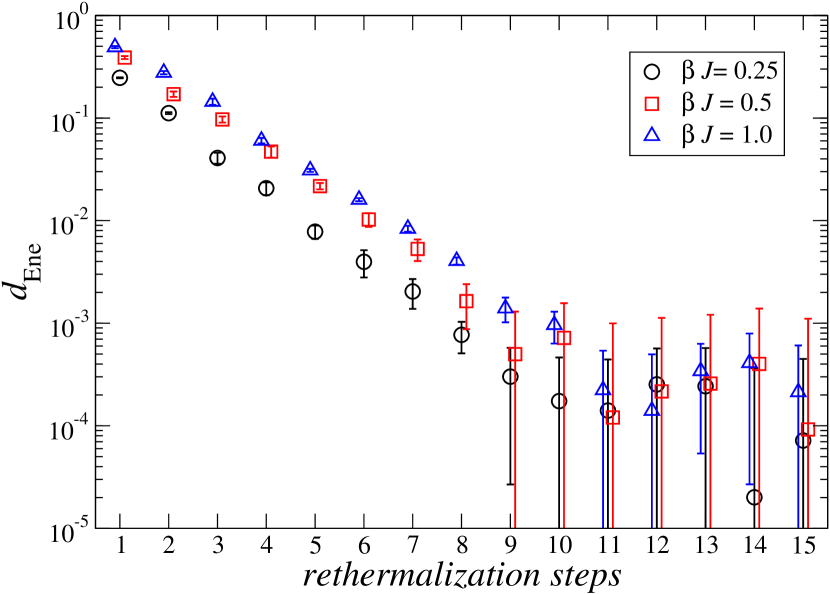
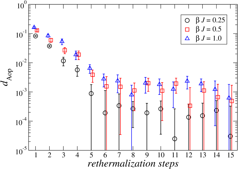
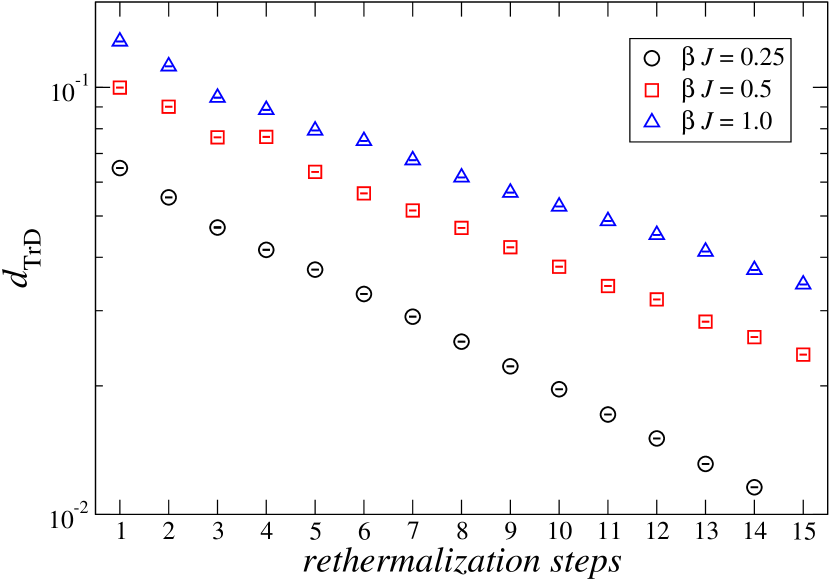
Figure 1: QMS: behavior of $d_{\text{Ene}}$ (top panel), $d_{\text{Aop}}$ (middle panel), and $d_{\text{TrD}}$ (lower panel), as a function of the number of rethermalization steps, for $\beta J=0.25,0.5$, and $1.0$.

Once a measurement of $A$ has been performed, two different strategies are possible: one can either restart the chain from the beginning or make the state (which is now an eigenstate of $A$) collapse back to an energy eigenstate (possibly different from the original one), by performing a QPE on the energy register followed by a measurement [26]. In the first case, the number of updates between different measurements is called thermalization time, while in the second case it is more natural to call it rethermalization time. As in Ref. [26], we follow the second strategy, which seems to be slightly more efficient.

The density matrix after the $i$-th rethermalization step is evaluated, before breaking the state with the $A$-measurement, by reading the state from the system register $\ket{\psi_{k(i)}}$ and building the projector $\rho_{i}\equiv\ket{\psi_{k(i)}}\bra{\psi_{k(i)}}$. Of course, any single instance of $\rho_{i}$ will be far from the exact density matrix $\rho_{\text{exact}}$, irrespective of the number of rethermalization steps. However, in the large sample limit, the (non-vanishing) discrepancy between $\bar{\rho}$ and $\rho_{\text{exact}}$ is only due to the systematic introduced by rethermalization and it is expected to vanish in the limit of an infinite number of rethermalization steps.

Results obtained for the three accuracy metrics $d_{\text{Ene}}$, $d_{\text{Aop}}$, and $d_{\text{TrD}}$ introduced in the previous section are shown in Fig. 1 (respectively top, middle, and bottom panel), for three values of the inverse temperature $\beta J=0.25,0.5$, and $1.0$. The statistics accumulated for the different points is not homogeneous, since runs have been stopped when $d_{\text{TrD}}$ reached a fixed accuracy. For this reason, runs performed at larger values of rethermalization steps, for which the bias is smaller, are significantly longer than the ones performed at smaller values. The stopping criterium adopted, together with the fact that $d_{\text{TrD}}$ is the most observable-independent among the adopted metrics, also explains why data reported in the top and central panel, respectively for $d_{\text{Ene}}$ and $d_{\text{Aop}}$, have significantly larger relative errors compared to those in the bottom panel, for $d_{\text{TrD}}$. It is also clear that, for all the metrics considered, the systematic bias approaches zero exponentially in the number of rethermalization steps, as expected on theoretical grounds.

IV.1.2 Quantum Quantum Metropolis Algorithm

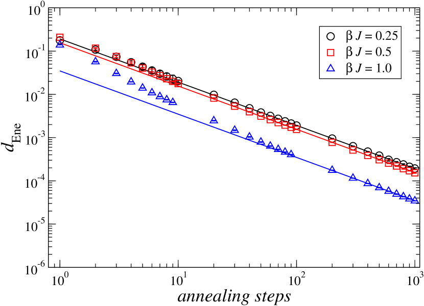
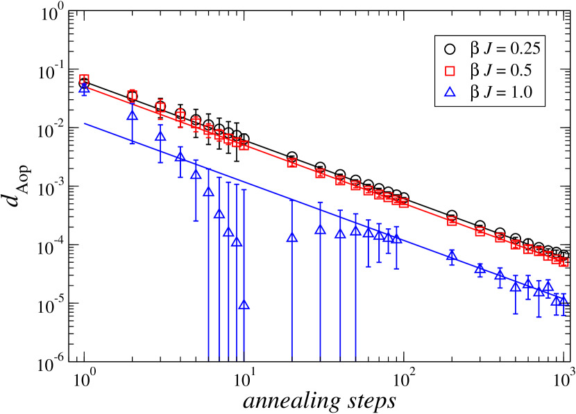
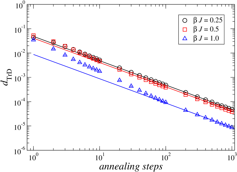
Figure 2: Q²MA: behavior of $d_{\text{Ene}}$ (top panel), $d_{\text{Aop}}$ (middle panel), and $d_{\text{TrD}}$ (bottom panel), as a function of the annealing steps $n_{a}$, for $\beta J=0.25,0.5$ and $1.0$, when using 3 qubits in the register $\ket{w}_{5}$, see Eq. (10). Continuous lines represent fits to the $1/n_{a}$ behavior, which well reproduces data at large enough $n_{a}$.

As explained in Sec. II.3, when using an exact energy representation, the systematic errors of the Q²MA algorithm are only due to the inexactness of the Szegedy QPE and to the finite number of annealing steps. However, we recall that it is generally not possible to make the Szegedy QPE exact, as the $W$ operator depends on $\beta$. Results presented in this section have been obtained by using the range $[0.5,1]$ for the Szegedy QPE (we are only interested to the eigenvalue 1) and fixing the number of qubits in the $\ket{w}_{5}$ register to 3, studying the dependence of systematic errors on the number of annealing steps. Consistent results are obtained when using 4 qubits for the register $\ket{w}_{5}$.

Contrary to what happens in the QMS case, it is not possible to measure $A$ and $E$ during the same run, and a new CETS reconstruction is required after each measurement. Since here we are only interested in systematics related to the incorrect determination of CETS, we evaluated the density matrix after each run of the algorithm, then exploiting the use of an emulator (rather than a real machine) to determine the exact average values of $A$ and $E$ corresponding to the given density matrix. Therefore, statistical errors shown in the following analysis are only due to fluctuations in the CETS determination from run to run, and are in fact small and well below the symbol size in most cases.

In Fig. 2, we present the results for $d_{\text{Ene}}$ (top panel), $d_{\text{Aop}}$ (middle panel), and $d_{\text{TrD}}$ (bottom panel) for the same three values of temperature explored in the previous subsection. In order to achieve a target precision on $d_{\text{TrD}}$, the runs performed with higher numbers of annealing steps required more Q²MA iterations, as the systematic error decreases with increasing steps. It can be observed that error bars are visible and not homogeneous only in the middle panel, where the systematic error also shows a non-monotonic behavior as a function of the number of annealing steps $n_{a}$: this is partially due to a change of sign in the bias of $A$ as a function of $n_{a}$, which occurs accidentally for this particular choice of parameters.

A clear difference of Fig. 2, with respect to Fig. 1, is that the scale is logarithmic on both axes. The reason is that in this case systematics appear to decrease polynomially (instead of exponentially) with the number of annealing steps. In particular, it is interesting to notice that, for large enough $n_{a}$, i.e., when the annealing step is small enough, data are well compatible with a $1/n_{a}$ behaviour. This result agrees with the prediction reported in Ref. [14] for a single and ergodic kick operator. However, in the light of the discussion reported in Sec. II, the result is far from trivial, and can be interpreted heuristically as evidence that, randomly alternating different kick operators in the different annealing steps, effectively reproduces, in the large annealing step limit, the ideal behaviour predicted for a single ergodic kick operator.

IV.2 Inexact energy representation

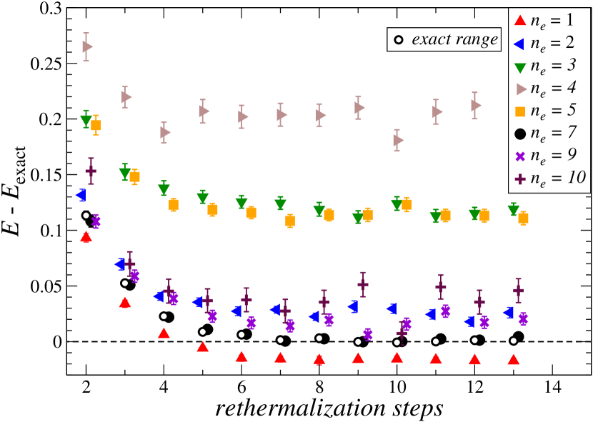
Figure 3: Energy discrepancy for the QMS algorithm with inexact QPE grid with fixed extrema $[-1.1,3.1]$ (in units of $J$) at $\beta J=0.25$.

In the previous analysis, working with an exact energy representation was instrumental to isolate some algorithmic-specific sources of systematical errors. This was possible because the considered quantum system has only two different exactly known energy levels, but it is clearly unrealistic in any case of direct physical interest. In such general cases, one has to use an inexact energy representation with $n_{e}$ qubit in the energy register(s), thus introducing further systemtatics.

Denoting by $E_{0}$ and $E_{1}$ the exact energy eigenstates of the frustrated triangle system (see Sec. III.1), we consider for the QPE an interval larger then $[E_{0},E_{1}]$ by an amount of about $2\delta$. Two natural prescriptions exist to place the $2^{n_{e}}$ grid points of the QPE: the “fixed extrema grid” and the “refined grid” cases.

In the “fixed extrema” case the inteval is fixed to be $[E_{0}-\delta,E_{1}+\delta]$ and the $2^{n_{e}}$ points are uniformly distributed in this interval. As $n_{e}$ is increased, the grid becomes finer, but the position of all the grid-points changes with $n_{e}$. On the other hand, in the “refined grid” case we use the interval

$$[E_{0}-\delta,E_{1}+\delta+(E_{1}-E_{0}+2\delta)(1-2^{1-n_{e}})]\ ,$$ (19)

which is chosen in such a way that, by increasing $n_{e}$, all points of the coarser grid are also present in the finer grid (with exception of the largest value).

Figure 3 shows the behavior of $\braket{E}$ as a function of the number of rethermalization steps for different values of $n_{e}$ in the “fixed extrema” scheme. It is clear that, for a large enough number of retermalization steps, a plateau emerges in $\braket{E}$, signaling the presence of a systematical difference between $\braket{E}$ and $\braket{E}_{\mathrm{exact}}$. This systematic is expected to vanish for $n_{e}\to\infty$, however the approach to the large $n_{e}$ limit is obviously non monotonic, at least in the range of $n_{e}$ values explored. This could make the diagnostic of the convergence non trivial in realistic cases, in which the exact expectation value is not known and the number of values of $n_{e}$ is limited by the hardware capability.

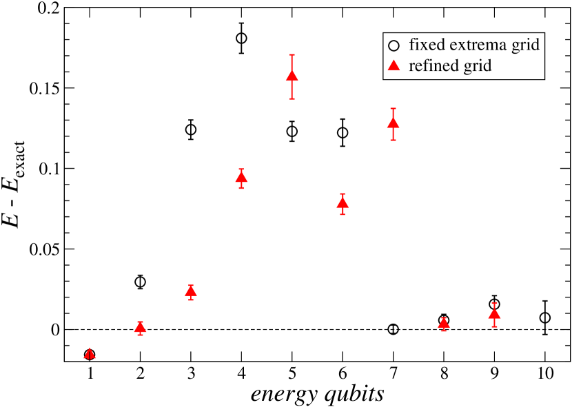
Figure 4: Effects of the two grid prescriptions for the QMS algorithm on energy discrepancies with inexact QPE grids at $\beta J=0.25$ and with 10 rethermalization steps.

For this reason we also investigated the “refined grid” method, which could be expected to have a smoother approach to the large $n_{e}$ limit. This is however not the case, as can be seen from Fig. 4, in which a comparison of two approaches is performed using 10 rethermalization steps (note that this number of retermalization steps is well in the plateau of Fig. 3). Both the approaches show a non monotonic scaling for an intermediate range of $n_{e}$ values, and converge to the correct asymptotic result for $n_{e}>8$. It is however reasonable to guess the non monotonic behaviour to continue also for larger values of $n_{e}$, where it is hidden by the statistical accuracy of our data.

The reason for the non monotonic behaviour is related to the fact that, for a given value of $n_{e}$, an eigenvalue can by chance be well-inside one of the QPE grid-interval or close to the boundary between two consecutive grid-intervals. Which of the two cases happen depends on $n_{e}$ and changes by increasing $n_{e}$, as can be seen in Fig. 5. Obviously the oscillations induced by this effect gets smaller and smaller as $n_{e}$ is increased, and ultimately convergence is reached with an arbitrary accuracy, but the approach to the asymptotic value presents oscillations. This effect is particularly evident in the system studied in this paper since the spectrum is very simple, consisting just of two points. In more complex systems, with a less simple spectrum, it seems reasonable to assume this discretization effect to be less significant, with some form of self-averaging happening.

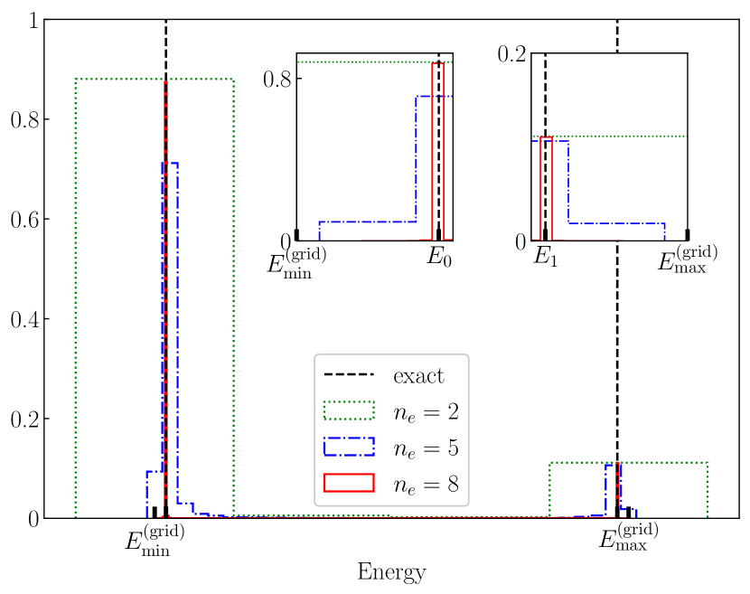
Figure 5: Comparison between the exact energy distribution and the one computed from the QMS using an energy grid in the QPE with fixed extrema and with inexact range $[E_{\min}^{(\mathrm{grid})},E_{\max}^{(\mathrm{grid})}]=[-1.1,3.1]$ (in units of $J$), for 3 values of the number of qubits of the energy register $n_{e}$. Figure refers in all cases to measures separated by 10 rethermalization steps. Insets provide a zoom over the regions close to the exact energy levels $E_{0}$ and $E_{1}$.

We tried to repeat a similar analysis to investigate the effect of an inexact energy representation also in the Q²MA case, however the results turned out to be much less clear, a fact that is probably due to several aspects. First of all the way in which energies enter the construction of the Szegedy operator is much more involved that the way in which they enter the Metropolis filter in the QMS algorithm, so “error propagation” is nontrivial for the limited number of qubits that can be used in the simulator. Another important point is the fact that in the Q²MA also other sources of systematics are present, like the discretization error in the Szegedy-related QPE, and different systematics can interact in a nontrivial way with each other. For this reason we were not able to identify a reasonable trend in our data for the case of the inexact energy representation in the Q²MA.

V Discussion and conclusions

This study is a step along a research line dedicated to the exploration of quantum algorithms for the computation of quantum thermal averages, in view of future applications to complex and interesting physical systems, like the fundamental theory of strong interactions, when technological developments will allow for reliable and scalable quantum machines.

In Ref. [26], some of the present authors already explored the Quantum Metropolis Sampling (QMS) algorithm and applied it to a frustrated three-spin system. In this case, we have considered the same physical system to develop a practical implementation of the Quantum-Quantum Metropolis Algorithm (Q²MA), proposed in Ref. [14]. This algorithm in principle represents a conceptual improvement over the QMS, as it enjoys a further quantum advantage. Such advantage stems from the fact that, while the QMS performs a Markov chain among the quantum states of the system which is classical in spirit and which faces the difficulties of the no-cloning theorem, the Q²MA acts like a quantum searching algorithm, where the searched state is the so-called CETS, which is a pure state in a doubled Hilbert space, whose amplitudes encode the thermal distribution of the target system. Provided that the CETS is found, the algorithm is exact in principle; however, an annealing procedure, in which one finds iteratively different CETS states corresponding to a descending sequence of temperatures, is used to improve the success probability of the searching algorithm.

A first result of our investigation is that the practical implementation of the Q²MA algorithm might be far less trivial. The searching algorithm is based on the construction of a Szegedy operator, which is assumed to have a single eigenstate with eigenvalue $\lambda=1$, corresponding to the CETS, which is actually the eigenstate the algorithm looks for. On the other hand, the construction of the Szegedy operator is based on the definition of a kick operator $K$, which is representative of a Markov chain and should be ergodic to guarantee the non-degeneracy of the $\lambda=1$ eigenstate: if this is not the case, the algorithm is not guaranteed to find the correct CETS, leading to possible systematics.

As we have discussed in Sec. II, finding an ergodic kick operator is a non-trivial assumption. However, a possible conceptual modification of the algorithm is to make use of different kick operators, which are randomly alternated during the annealing procedure: even if the single kick operators are non-ergodic, the fact that CETS corresponding to close enough temperatures have a good overlap is expected to strongly enhance the probability that the correct CETS is found along the annealing sequence, at least if the annealing step is small enough.

As we have shown, this conceptual modification works well in practice, so that one is able to reproduce quantum thermal averages through the annealing with different kick operators; on the contrary, using a single non-ergodic operators does not work. However, a consequence of this modification is that now the annealing step, or in other words the number of annealing steps $n_{a}$, is not only relevant to the success probability (i.e., of finding an eigenstate of the Szegedy operator with eigenvalue 1) but also to the fact that the selected state is actually the CETS. In other words, there is a systematic effect in the algorithm, related to the fact that one might find the wrong state, and this systematic is a function of $n_{a}$. In particular, we have shown that the error scales as $1/n_{a}$, at least for $n_{a}$ large enough.

Going back to the comparison with the QMS, the final situation seems different from initial expectations. In the QMS, the main algorithm-specific systematics is related to the number of rethermalization steps performed along the Markov chain: in this case, the systematic error is exponentially suppressed in such number. The outcome of our study is that the main algorithm-specific systematics of Q²MA scales as the inverse of the number of annealing steps, which is a less favorable polynomial scaling, compared to QMS.

Finally, we have explored the systematic effects related to the inexact representation of the system energy spectrum obtained through the Quantum Phase Estimation (QPE), which is a problem affecting a large class of quantum algorithms and could be avoided for the particular explored system, due to its simplicity. In this case, the systematic error is expected to be suppressed as the number of qubits used to represent the energy register is increased, i.e., as the grid of possible outcomes of the QPE is made finer and finer. We have shown that this is indeed the case when the number of qubits is large enough, with a non-trivial intermediate regime due to the interplay between the energy level spacing, the grid spacing and overall range explorable by QPE. As a final comment, one should consider that this intermediate regime is likely to be less relevant for real and more complex many-body systems, for which the distribution of energy levels is more chaotic.

Future developments along the same research line should consider and compare different approaches, like those based on variational quantum algorithms or on quantum simulators [35], as well as less trivial models, including gauge degrees of freedom.