Quasinormal modes of the Schwarzchild black hole with a deficit solid angle and quintessence-like matter: Scalar and electromagnetic perturbations

Abstract

We study the quasinormal modes (QNM) for scalar, and electromagnetic perturbations in the Schwarzchild black hole with a deficit solid angle and quintessence-like matter. Using the sixth–order WKB approximation and the improved asymptotic iteration method (AIM) we can determine the dependence of the quasinormal modes on the parameters of the black hole and the parameters on the test fields. The values of the real part and imaginary parts of the quasi–normal modes increase with the decrease of the values of the deficit solid angle and density of quintessence-like matter. The quasinormal modes gotten by these two methods are in good agreement. Using the finite difference method, we obtain the time evolution profile of such perturbations in this Black Hole.

Keywords: Quasi–normal modes, Quintessence-like matte, WKB approximation, AIM.

I Introduction

One state resulting from the disturbance (scalar or electromagnetic perturbations) of a black hole (BH) is an oscillation with complex frequencies called quasinormal modes (QNM). The QNM is related to the parameters that describe the BH as mass, charge, angular moment, and others. But also, we can analyze the frequency of oscillation and the damping of the oscillation through the real part and imaginary part of the frequencies of the QNM respectively. Another important contribution of the QNM is the analysis of the stability of the BHs and their gravitational radiation.

The study of QNM has been carried out for different solutions of black holes that represent isolated solutions or in vacuum for example; QNM of Schwarzschild Iyer:1986nq , Reissner–Nordström, Hayward Lin:2013 , and others. Also, different authors have investigated QNM in non-linear electrodynamics (NLED); QNM of Bardeen Fernando:2012yw , Einstein-Born-Infeld Lee:2020iau , and Generic-class Lopez:2022uie to mention some investigations. Considering that the black holes coexistence with other types of matter or energy is significant the studies of QNM of BHs surrounded by the quintessence have been developed for different scenarios as Hayward Pedraza:2021hzw , Bardeen, Schwarzschild Zhang:2006ij , Reissner–Nordström Saleh:2011zz and others black holes, all surrounded by quintessence (using the Kiselev model Kiselev:2002dx ).

There are different models as candidates for dark energy. One of the candidates is the quintessence that differs from the cosmological constant in the magnitude of the state parameter that represents the ratio of pressure to the energy density of dark energy. The QNMs of a Schwarzschild black hole with a deficit angle and quintessence-like matter are investigated in Yu:2022yyv .

In the works above mentioned on the study of QNM, different numerical methods have been applied being the WKB method the most used. When you want to perform the analysis of QNM, this lead to a wave equation with a specific effective potential, depending on the characteristics of the effective potential some numerical methods are more suitable.

The asymptotic iteration method (AIM) proposed in HakanCiftci_2003 to obtain the eigenvalues and eigenfunctions of linear differential equations second-order homogeneous, has shown is a method can be a technique efficient and accurate in calculating the frequencies of QNMs for a wide variety of black holes, for example in Cho:2011sf the QNMS of Schwarzschild, Schwarzschild anti-de Sitter or de Sitter, Reissner–Nordström and Kerr are analyzed with AIM. When you want to perform the analysis of QNM, this lead to a wave equation with a specific effective potential, depending on the characteristics of the effective potential some numerical methods are more suitable.

This paper is devoted to the study of the QNMs and the time evolution of massless scalar and electromagnetic perturbations on Schwarzchild black hole with a deficit solid angle and quintessence-like matter. The wave-like perturbation equation, with an effective potential, can be solved to calculate the QNMs numerically by two methods: the WKB approach and AIM. The paper is organized as follows: Section II we present the Black Hole considered in the present work and we briefly discuss the event horizons. In Sec. III we describe the scalar and electromagnetic perturbations of a Black Hole. We study the behavior of effective potential for different perturbations considering the special cases when the quintessence state parameter takes the values -1/2 and -2/3. In Sec. IV we present the results for quasinormal frequencies (QMFs) and in Sec.V we present the time domain analysis. Finally, our conclusions are in Sec. VI.

II A Schwarzchild black hole with quintessence-like matter and a deficit solid angle

Barriola and Vilenkin Barriola:1989hx proposed static and spherical symmetric solution that describe Schwarzchild Black Hole with a deficit solid angle and quintessence-like matter. This solution is given by

$$ds^{2}=f(r)dt^{2}-\frac{dr^{2}}{f(r)}-r^{2}d\theta^{2}-r^{2}\sin^{2}\theta d\phi^{2}\,,$$ (1)

where

$$f(r)=1-\frac{2M}{r}-\epsilon^{2}+\frac{\rho_{0}}{3\omega_{0}r^{3\omega_{0}+1}}\,.$$ (2)

In which $\epsilon$ is the deficit solid angle parameter, $\rho_{0}$ is the density of quintessence-like matter, $\omega_{0}$ is the quintessence state parameter and satisfies $-1<\omega_{0}<-1/3$ and $M$ is the black hole mass. When $\epsilon=\rho_{0}=0$ the metric function $f(r)$ is reduced to the solution of Schwarzschild. The solution (2) asymptotically behave as the AdS-like space-time one at larges distances $r\to\infty$

$$\lim_{r\to\infty}f(r)\approx-\frac{\rho_{0}\left(1-\epsilon^{2}\right)}{3\left|\omega_{0}\right|}r^{3\left|\omega_{0}\right|-1}+\dots\,.$$ (3)

The horizons of Schwarzchild with quintessence-like matter and a deficit solid angle (Schwdm) are determined by the positive roots of the equation $f(r)=0$, this condition leads to the polynomial

$$3\omega_{0}\left(\epsilon^{2}-1\right)r^{3\omega_{0}+1}+6M\omega_{0}r^{3\omega_{0}}-\rho_{0}=0\,.$$ (4)

The number of horizons depends entirely on the choice of the values of parameters $\epsilon$, $\omega_{0}$, $M$ and $\rho_{0}$. However, in an appropriated parametric region, the solution has two horizons: the event horizon $r_{+}$ and the cosmological horizon $r_{c}$. Using the ideas of Liu:2020evp , here hereafter, we fix the event horizon in $r_{+}=1$. To ensure $f(r_{+})=0$, it is required that the mass parameter can be expressed as

$$M=\frac{3\omega_{0}\left(1-\epsilon^{2}\right)+\rho_{0}}{6\omega_{0}}\,.$$ (5)

The region parametric in which the Schwdm BH has event horizon $r_{+}$ and cosmological horizon $r_{c}$ are allowed ,can be determined by $f^{\prime}(r_{+})>0$. This condition leads to the next expression;

$$\rho_{0}<1-\epsilon^{2}\,.$$ (6)

The region plot of the allowed parameter region is given in Fig. 1(a). For all values of ($\epsilon^{2},\rho_{0}$) in region shaded, there are two real positive roots of Eq. (4), $r_{+}=1$ and $r_{c}$, which satisfy $r_{+}\leq r_{c}$. On the other hand, for values of ($\epsilon^{2},\rho_{0}=1-\epsilon^{2}$) corresponding to the line represents extremal Schwdm BH, where $r_{+}=r_{c}=1$. In the Fig. 1(a) we observe that the parametric region is independent of $\omega_{0}$. From Fig. 1(b), we plot the metric function $f(r)$ for different values of $\omega_{0}$ and we can conclude that the quintessence horizon is very large for $\omega_{0}\to-1/3$.

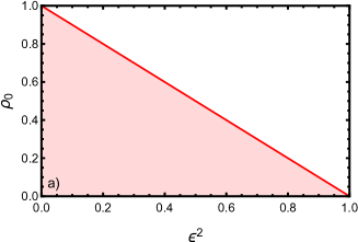
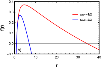
Figure 1: a) The parametric region where the Schwdm BH has two horizons, $r_{+}\leq r_{c}$ according to $\omega_{0}$ values. The region is bounded by the line $(\rho_{0}=1-\epsilon^{2})$, $\rho_{0}=0$ and $\epsilon=0$ (the region shaded). b) The graph shows the metric function (2) as function of $r$ for different values of $\omega_{0}$. Here $\rho_{0}=0.2$ and $\epsilon^{2}=0.2$.

inserting $M$ (5) into (2), we can write the metric function as

$$f(r)=1-\epsilon^{2}-\frac{1-\epsilon^{2}+\frac{\rho_{0}}{3\omega_{0}}}{r}+\frac{\rho_{0}}{3\omega_{0}r^{3\omega_{0}+1}}\,.$$ (7)

For the particular case $\omega_{0}=-2/3$, the cosmological and event horizons are given by

$$r_{+}=1,\quad r_{c}=\frac{2\left(1-\epsilon^{2}\right)-\rho_{0}}{\rho_{0}}\,.$$ (8)

And for $\omega_{0}=-1/2$, we get

$$r_{+}=1,\quad r_{c}=\frac{\left(3\left[1-\epsilon^{2}\right]-2\rho_{0}\right)}{2\rho_{0}}\left(1+\frac{3\left[1-\epsilon^{2}\right]-2\rho_{0}+\sqrt{3\left(3\left[1-\epsilon^{2}\right]-2\rho_{0}\right)\left(1-\epsilon^{2}+2\rho_{0}\right)}}{4\rho_{0}}\right)\,.$$ (9)

When the event and cosmological horizons coincide with each other, the Schwdm BH is an extremal one ($\rho_{0}=1-\epsilon^{2}$),thus $r_{+}=r_{c}=1$.

To conclude this section, it is worth mentioning that if $r_{+}\neq 1$ then expression (6) takes the following form

$$\rho_{0}<\left(1-\epsilon^{2}\right)\left[\frac{\left(1-\epsilon^{2}\right)\left(3|\omega_{0}|-1\right)}{6M|\omega_{0}|}\right]^{3|\omega_{0}|-1}\,,$$ (10)

for further discussion, see the Ref. Yu:2022yyv . Which depends explicitly on $\omega_{0}$, so comparing the different parametric regions, it is possible to mention that the parametric region for $\omega_{0}=-2/3$ is much smaller than the parametric region for $\omega_{0}=-1/2$.

III Scalar and Electromagnetic perturbations

In this section, we briefly show the behavior of scalar and electromagnetic perturbations in a Black Hole with a deficit solid angle and quintessence-like matter, following the Refs. Xi:2010pv ; Wang:2012vvx . The propagation of a scalar field in a curved background is described by the Klein-Gordon equation

$$\frac{1}{\sqrt{-g}}\partial_{\mu}\left(\sqrt{-g}\,g^{\mu\nu}\partial_{\nu}\Psi\right)=0\,.$$ (11)

We separate variables by setting

$$\Psi(t,r,\theta,\phi)=\frac{1}{r}\phi_{s}(r)Y_{lm}(\theta,\phi)e^{i\omega t}\,,$$ (12)

where $Y_{lm}(\theta,\phi)$ are the spherical harmonics. Substituting Eq. (12) into (11), we get the next radial equation

$$\left[\frac{d^{2}}{dr_{*}^{2}}+\omega^{2}-V_{s}(r)\right]\phi_{s}(r)\,,$$ (13)

where $r_{*}$ is the tortoise coordinate

$$dr_{*}=\frac{dr}{f(r)}\,,$$ (14)

and $V_{s}(r)$ is the effective potential

$$V_{s}=f(r)\left[\frac{l(l+1)}{r^{2}}+\frac{2\left[\frac{3\omega_{0}\left(1-\epsilon^{2}\right)+\rho_{0}}{6\omega_{0}}\right]}{r^{3}}-\frac{\rho_{0}\left(3\omega_{0}+1\right)}{3\omega_{0}r^{3\omega_{0}+3}}\right]\,,$$ (15)

whereas, the electromagnetic field in curved space follows the next equation

$$\frac{1}{\sqrt{-g}}\partial_{\mu}\left(\sqrt{-g}\,F_{\beta\gamma}g^{\beta\nu}g^{\gamma\mu}\right)=0\,,$$ (16)

where $F_{\beta\gamma}=\partial_{\beta}A_{\gamma}-\partial_{\gamma}A_{\beta}$ and the vector potential $A_{\mu}$ can be expressed as

$$A_{0}=A_{1}=A_{2}=0,\quad A_{3}=\phi_{e}(r)\sin(\omega t)\sin\theta\frac{dP_{l}(\cos\theta)}{d\theta}\,.$$ (17)

After separation of variables, the radial parts of the electromagnetic field perturbation equation takes the form similar to (13), but the effective potential is given by

$$V_{e}=f(r)\frac{l(l+1)}{r^{2}}\,.$$ (18)

From Eqs. (15) and (18), the scalar and electromagnetic perturbations can be described by a Schrödinger-like equation with potential

$$V(r)=f(r)\left[\frac{l(l+1)}{r^{2}}+(1-s^{2})\frac{2m(r)}{r^{3}}+(1-s)\left(\frac{f^{\prime}(r)}{r}-\frac{2m(r)}{r^{3}}\right)\right]\,,$$ (19)

where

$$m(r)=\frac{3\omega_{0}\left(1-\epsilon^{2}\right)+\rho_{0}}{6\omega_{0}}-\frac{\rho_{0}}{6\omega_{0}r^{3\omega_{0}}}\,,$$ (20)

and $l$ is the multipole number ($\l\geq s$), $s$ is the spin of the perturbative field: $s=0$ corresponding to scalar perturbation and $s=1$ to electromagnetic perturbation. The effective potential (19) has asymptotic value $V(r)\approx\rho_{0}^{2}\left(s-1\right)\left(1+s+3\omega_{0}\right)/\left(9\omega_{0}^{2}r^{6\omega_{0}+4}\right)$ when $r\to\infty$. From this behavior asymptotic for the effective potential, we can see that if $\omega_{0}<-2/3$, $V\to\infty$ when $r\to\infty$. Thus we only study the case where the state parameter which has the range $-2/3\leq\omega_{0}<-1/3$. For the specific case $\omega_{0}=-2/3$, the scalar perturbation, $V(r)\approx\rho_{0}^{2}/4$.

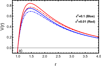
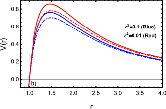
Figure 2: a) The behavior of the effective potential for $\omega_{q}=-2/3$ is shown for various values of $\epsilon^{2}$, with $\rho_{0}=0.1$ and $l=2$. b) The behavior of the effective potential for $\omega_{q}=-1/2$ is shown for various values of $\epsilon^{2}$, with $\rho_{0}=0.1$ and $l=2$. In both figures, the effective potential of scalar (solid) and electromagnetic (dot dashed)

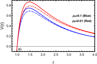
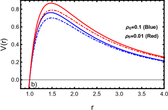
Figure 3: a) The behavior of the effective potential for $\omega_{q}=-2/3$ is shown for various values of $\rho_{0}$, with $\epsilon^{2}=0.1$ and $l=2$. b) The behavior of the effective potential for $\omega_{q}=-1/2$ is shown for various values of $\rho_{0}$, with $\epsilon^{2}=0.1$ and $l=2$. In both figures, the effective potential of scalar (solid) and electromagnetic (dot dashed)

The behavior of $V(r)$ for different values of $\epsilon^{2}$ is described in Fig. 2 a) and b) for $\omega_{q}=-2/3$ and $\omega_{q}=-1/2$ respectively, while the behavior of effective potential for different values of $\rho_{0}$ is described in Fig. 3 for different values of state parameter. It is worth mentioning that effective potential is positive definite for $r_{*}\in\left[-\infty,\infty\right]$ and have a potential barrier near the event horizon for very small values of the state parameter and deficit solid angle parameter.

From Figs. 2 and 3 we can mention that in both case $V_{\text{elec}}(r)<V_{\text{sc}}(r)$.

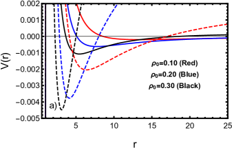
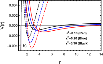
Figure 4: The effective potential of scalar field with $l=0$ mode. The a) and b) plots correspond to $\epsilon^{2}=0.1$ and $\rho=0.35$ respectively. In both figures, the effective potential for $\omega_{0}=-1/2$ is represented by the solid line and by the dotted line for $\omega_{0}=-2/3$.

If we study the effective potential for scalar field with $l=0$ mode, we can see that $V(r)$ can take negative values between r₊ and $r_{c}$ (see Figs. 4(a) and 4(b)). This potential well is the key point for the occurrence of instability. However, the negative effective potential does not guarantee that the part imaginary of the quasinormal frequencies takes positive values e.i. the existence of a negative potential well can be viewed as the necessary but not sufficient condition for instability PhysRevD.86.024028 .

In Fig. 4(a) shows the mode $l=0$ for the scalar field for different values of $\rho_{0}$, we can see that for increasing values of $\rho_{0}$, the depth of the potential well increases, while in Fig. 4(b) shows that for increasing values of $\epsilon^{2}$, the depth of the potential well decreases.

The Eq. (13) exhibits the following behavior near the horizons

$$\phi_{s}\approx\begin{cases}e^{-i\omega r_{*}},&r_{*}\to-\infty\,(r\to r_{+})\\ e^{i\omega r_{*}},&r_{*}\to\infty\,(r\to r_{c})\end{cases}\,,$$ (21)

the asymptotic solutions (21) imply that the wave at the event horizon is purely incoming, whereas at the cosmological horizon is purely outgoing. For the boundary condition mentioned above, the wave equation (13) can be solved in order to obtain the spectrum of the quasi normal frequencies.

IV Quasinormal modes using the improved AIM

The AIM method has been used for to calculate the QNMs of black holes in the asymptotic dS spacetimes Cho:2011sf ; Cho:2009cj To apply AIM, we need to introducing the transformation of coordinates $\xi=1/r$. In the new coordinate $\xi$, the equations (13), which leads to the following expression

$$\left[\frac{d^{2}}{d\xi^{2}}+\frac{p^{\prime}}{p}\frac{d}{d\xi}+\frac{\omega^{2}}{p^{2}}-\frac{l\left(l+1\right)+\left(1-s^{2}\right)\left(1-\epsilon^{2}-\frac{p}{\xi^{2}}\right)-\left(1-s\right)\rho_{0}\xi^{3\omega_{0}+1}}{p}\right]\phi=0\,,$$ (22)

where the prime denotes derivative with respect $\xi$, and $p(\xi)$ is defined as

$$p(\xi)=\left(1-\epsilon^{2}\right)\xi^{2}-\frac{3\omega_{0}\left(1-\epsilon^{2}\right)+\rho_{0}}{3\omega_{0}}\xi^{3}+\frac{\rho_{0}}{3\omega_{0}}\xi^{3(\omega_{0}+1)}\,,$$ (23)

To accommodate the outgoing wave boundary condition $\phi\to e^{i\omega r_{*}}$ in terms of $\xi$, we define

$$e^{i\omega r_{*}}=e^{-i\omega\int\frac{d\xi}{p(\xi)}}\,.$$ (24)

The expression (24) scale out the divergence behavior at the cosmological horizon. So, by implement the boundary conditions in the AIM method, we redefine the function $\phi$ in terms of the a new function $\chi$. So we can write

$$\phi\left(\xi\right)=e^{-i\omega\int\frac{d\xi}{p(\xi)}}\left(\xi-\xi_{+}\right)^{-i\omega/\kappa_{+}}\chi\left(\xi\right)\,.$$ (25)

Considering (25), we can scale out the divergent behavior at the event horizon. Here $\kappa_{+}$ is the surface gravity at the horizon defined as;

$$\kappa_{+}=\left.\frac{1}{2}\frac{d}{dr}f(r)\right|_{r\to r_{+}}=-\left.\frac{\xi^{2}}{2}\frac{d}{d\xi}f(\xi)\right|_{\xi\to\xi_{+}}\,.$$ (26)

By combining equations (22) and (25), we obtain the following differential equation for $\chi(\xi)$

$$\frac{d^{2}\chi\left(\xi\right)}{d\xi^{2}}=\lambda_{0}\left(\xi\right)\frac{d\chi\left(\xi\right)}{d\xi}+s_{0}\left(\xi\right)\chi\left(\xi\right)\,,$$ (27)

where

$$\lambda_{0}\left(\xi\right) = \frac{2i\omega}{\kappa_{+}\left(\xi-\xi_{+}\right)}-\frac{p^{\prime}-2i\omega}{p}\,,$$ (28)

$$s_{0}\left(\xi\right) = \frac{l\left(l+1\right)+\left(1-s^{2}\right)\left(1-\epsilon^{2}-\frac{p}{\xi^{2}}\right)-\left(1-s\right)\rho_{0}\xi^{3\omega_{0}+1}}{p}-\frac{i\omega\left(\kappa_{+}+i\omega\right)}{\kappa^{2}_{+}\left(\xi-\xi_{+}\right)^{2}}+\frac{i\omega\left(p^{\prime}-2i\omega\right)}{p\kappa_{+}\left(\xi-\xi_{+}\right)}\,.$$ (29)

Using the expression (28) and (29) in the recurrence relations (42) and (43) (see Appendix) to calculate the quantities that appear in the quantization condition (46). The stable roots of condition (46) are the QNMs of the scalar and electromagnetic test fields. We use Mathematica Software to perform all the calculations.

We present in Tables 1, 2, 3 and 4 results for scalar and electromagnetical perturbation respectively. We compared our results obtained using AIM (after of fifteen iterations) with WKB to sixth-order.

Scalar perturbations
		$\omega_{q}=-2/3$			$\omega_{q}=-1/2$
		WKB		AIM		WKB		AIM
$\epsilon^{2}$	$l=0$
0.01		0.187043-0.191982$i$		0.186947-0.195326$i$		0.190396-0.184349$i$		0.190432-0.189805$i$
0.10		0.166671-0.174322$i$		0.167064-0.176485$i$		0.170528-0.166209$i$		0.170589-0.170975$i$
$\epsilon^{2}$	$l=1$
0.01		0.536367-0.175563$i$		0.536404-0.175406$i$		0.542744-0.174016$i$		0.542784-0.173865$i$
0.10		0.504477-0.15763$i$		0.504505-0.157515$i$		0.510936-0.156189$i$		0.510967-0.156078$i$
	$l=3$
0.01		1.252810-0.172128$i$		1.252810-0.172127$i$		1.263260-0.171518$i$		1.263260-0.171517$i$
0.10		1.184560-0.154697$i$		1.184560-0.154696$i$		1.195430-0.154106$i$		1.195430-0.154105$i$
	$l=5$
0.01		1.969140-0.171672$i$		1.969140-0.171672$i$		1.984550-0.171193$i$		1.984550-0.171193$i$
0.10		1.863150-0.154311$i$		1.863150-0.154311$i$		1.879280-0.153837$i$		1.879280-0.153837$i$
	$l=7$
0.01		2.685400-0.171528$i$		2.685400-0.171528$i$		2.705960-0.171091$i$		2.705960-0.171091$i$
0.10		2.541410-0.154190$i$		2.541410-0.154190$i$		2.562970-0.153753$i$		2.562970-0.153753$i$

Table 1: Quasinormal frequencies for the Scalar perturbations for several values of the parameter $\epsilon^{2}$, with $n=0$ and $\rho_{0}=0.1$.

Scalar perturbations
		$\omega_{q}=-2/3$			$\omega_{q}=-1/2$
		WKB		AIM		WKB		AIM
$\rho_{0}$	$l=0$
0.01		0.195563-0.180831$i$		0.195457-0.187169$i$		0.195975-0.179954$i$		0.195743-0.186603$i$
0.10		0.166671-0.174322$i$		0.167064-0.176485$i$		0.170528-0.166209$i$		0.170589-0.170975$i$
$\rho_{0}$	$l=1$
0.01		0.547237-0.173928$i$		0.547278-0.173778$i$		0.547896-0.173768$i$		0.547937-0.173619$i$
0.10		0.504477-0.157630$i$		0.504505-0.157515$i$		0.510936-0.156189$i$		0.510967-0.156078$i$
	$l=3$
0.01		1.270480-0.171755$i$		1.270480-0.171753$i$		1.271550-0.171696$i$		1.271550-0.171695$i$
0.10		1.184560-0.154697$i$		1.184560-0.154696$i$		1.195430-0.154106$i$		1.195430-0.154105$i$
	$l=5$
0.01		1.995190-0.171473$i$		1.995190-0.171473$i$		1.996760-0.171429$i$		1.996760-0.171429$i$
0.10		1.863150-0.154311$i$		1.863150-0.154311$i$		1.879280-0.153837$i$		1.879280-0.153837$i$
	$l=7$
0.01		2.720170-0.171385$i$		2.720170-0.171385$i$		2.722270-0.171345$i$		2.722270-0.171345$i$
0.10		2.541410-0.154190$i$		2.541410-0.154190$i$		2.562970-0.153753$i$		2.562970-0.153753$i$

Table 2: Quasinormal frequencies for the Scalar perturbations for several values of the parameter $\rho_{0}$, with $n=0$ and $\epsilon^{2}=0.1$.

Electromagnetic perturbations
		$\omega_{q}=-2/3$			$\omega_{q}=-1/2$
		WKB		AIM		WKB		AIM
$\epsilon^{2}$	$l=1$
0.01		0.465629-0.165506 $i$		0.465727-0.165296$i$		0.469719-0.165173$i$		0.469814-0.164968$i$
0.10		0.444590-0.149292 $i$		0.444653-0.149151$i$		0.448856-0.148948$i$		0.448918-0.148810$i$
	$l=3$
0.01		1.223820-0.170371$i$		1.223820-0.170370$i$		1.233200-0.169992$i$		1.233200-0.169991$i$
0.10		1.160040-0.153247$i$		1.160040-0.153246$i$		1.169890-0.152861$i$		1.169890-0.152860$i$
	$l=5$
0.01		1.950800-0.170964$i$		1.950800-0.170964$i$		1.965510-0.170580$i$		1.965510-0.170580$i$
0.10		1.847640-0.153727$i$		1.847640-0.153727$i$		1.863110-0.153337$i$		1.879280-0.153837$i$
	$l=7$
0.01		2.671970-0.171148$i$		2.671970-0.171148$i$		2.692020-0.170762$i$		2.692020-0.170762$i$
0.10		2.530050-0.153876$i$		2.530050-0.153876$i$		2.551140-0.153484$i$		2.551140-0.153484$i$

Table 3: Quasinormal frequencies for the Electromagnetic perturbations for several values of the parameter $\epsilon$, with $n=0$ and $\rho_{0}=0.1$.

Electromagnetic perturbations
		$\omega_{q}=-2/3$			$\omega_{q}=-1/2$
		WKB		AIM		WKB		AIM
$\rho_{0}$	$l=1$
0.01		0.472513-0.165563$i$		0.472604-0.165367$i$		0.472932-0.165534 $i$		0.473022-0.165339$i$
0.10		0.444590-0.149292$i$		0.444653-0.149151$i$		0.448856-0.148948$i$		0.448918-0.148810$i$
	$l=3$
0.01		1.239670-0.170316$i$		1.239670-0.170314$i$		1.240630-0.170282$i$		1.240630-0.170281$i$
0.10		1.160040-0.153247$i$		1.160040-0.153246$i$		1.169890-0.152861$i$		1.169890-0.152860$i$
	$l=5$
0.01		1.975680-0.170895$i$		1.975680-0.170895$i$		1.977180-0.170861 $i$		1.977180-0.170861$i$
0.10		1.847640-0.153727$i$		1.847640-0.153727$i$		1.863110-0.153337$i$		1.863110-0.153337$i$
	$l=7$
0.01		2.705880-0.171074$i$		2.705880-0.171074$i$		2.707920-0.171041$i$		2.707920-0.171041$i$
0.10		2.530050-0.153876$i$		2.530050-0.153876$i$		2.551140-0.153484$i$		2.551140-0.153484$i$

Table 4: Quasinormal frequencies for the Electromagnetic perturbations for several values of the parameter $\rho_{0}$, with $n=0$ and $\epsilon^{2}=0.1$.

In Table 1 and Table 3, we can observe the frequencies of the QNMs for the scalar and electromagnetic perturbations, the real part increases when $l$ increases when we fix the parameter $\rho_{0}$. The same behavior occurs when the parameter $\epsilon$ is fixed (see Tables 2 and 4 ). In the cases of the imaginary part when the parameters $\rho_{0}$ or $\epsilon$ are fixed, their values increases as $l$ increases, for both perturbations, then we can mention that the relaxation time of the Schwdm BH diminishes and the BH is stable.

It can be seen that the range of real and imaginary frequencies is approximately the same and it does not change drastically when the WKB or the AIM methods are considered, so the AIM method is very reliable.

V Time evolution of Scalar and Electromagnetic perturbations

In this section we compute the time evolution of the Scalar and Electromagnetic perturbations to further reveal the instability of the Schwarzchild black hole with quintessence-like matter and a deficit solid angle. For the time evolution, the radial part of the perturbation equations are reduced to the form

$$\frac{\partial^{2}\Psi}{\partial t^{2}}-\frac{\partial^{2}\Psi}{\partial r_{*}^{2}}+V(r)\Psi=0\,.$$ (30)

After recasting the wave equation (30) in the null coordinates $u=t-r_{*}$ and $v=t+r_{*}$ we obtain

$$-4\frac{\partial^{2}}{\partial u\partial v}\Psi(u,v)=V(u,v)\Psi(u,v)$$ (31)

In order to compute the time evolution of $\Psi$ we implemented the discretization scheme developed in Gundlach:1993tp i.e. we can numerically integrate by using the finite difference method. Using the Taylor expansion, one find

$$\Psi(u+\Delta u,v+\Delta v) = \Psi(u,v+\Delta v)+\Psi(u+\Delta u,v)-\Psi(u,v)$$ (32)

$$-\frac{\Delta u\Delta v}{8}V\left(\frac{2v-2u+\Delta v-\Delta u}{4}\right)\left[\Psi(u+\Delta u,v)+\Psi(u,v+\Delta v)\right]+O\left(h^{4}\right)\,,$$

where $h$ is an overall grid scalar factor ($\Delta u=\Delta v=h$). To perform the numerical integration on an uniformly spaced grid. we impose the following initial profile

$$\Psi\left(u,v=0\right)=0,\qquad\psi\left(u=0,v\right)=Ae^{-\frac{\left(v-v_{0}\right)^{2}}{2\sigma^{2}}}\,,$$ (33)

since the late-time behavior of the wave function is found to be insensitive to the initial data, we set the initial Gaussian distribution with width, $\sigma=3$ centered at $v_{0}=10$, amplitude $A=1$ and with an overall grid scale factor $h=0.2$. To proceed the integration in the aforementioned scheme one has to find the value of the potential at $r(r_{*})$ at each step.

For the special case $\omega_{0}=-2/3$, we get

$$r_{*}=\frac{1}{2\kappa_{+}}\ln\left|\frac{r}{r_{+}}-1\right|+\frac{1}{2\kappa_{c}}\ln\left|1-\frac{r}{r_{c}}\right|\,,$$ (34)

and for $\omega_{0}=-1/2$, we obtain

$$r_{*}=-\frac{3\sqrt{r}}{\rho_{0}}-\frac{1}{2\kappa_{+}}\ln\left|\frac{\sqrt{r}}{r_{+}}-1\right|-\frac{3r_{1}^{3}}{\rho_{0}\left(r_{1}-1\right)\left(r_{1}-r_{2}\right)}\ln\left|1-\frac{\sqrt{r}}{r_{1}}\right|+\frac{3r_{2}^{3}}{\rho_{0}\left(r_{2}-1\right)\left(r_{1}-r_{2}\right)}\ln\left|1-\frac{\sqrt{r}}{r_{2}}\right|\,,$$ (35)

where

$$r_{1,2}=\frac{1}{4\rho_{0}}\left[3\left(1-\epsilon^{2}\right)-2\rho_{0}\pm\sqrt{3\left[3\left(1-\epsilon^{2}\right)-2\rho_{0}\right]\left[1-\epsilon^{2}+2\rho_{0}\right]}\right]\,,$$ (36)

So we get $r(r_{*})$ numerically, using the built-in Mathematica commands.

In Fig. 5 we show the evolution profile of the scalar field for $l=0$ mode. We observe that the $\mathrm{Log}\left|\Psi\right|$ linearly depends on $t$ at later times. From Fig. 5(a) we see that the perturbations start to become unstable for higher values of $\rho_{0}$, whereas if the values of $\epsilon^{2}$ increase, the system becomes stable. In both graphs when the value of the quintessence parameter $\omega_{0}$ increases, the system becomes more stable, which is in correspondence with the peculiar shape of potential for $\omega_{0}=-2/3$ and $\omega_{0}=-1/2$ (Fig. 4).

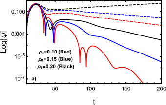
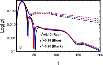
Figure 5: Logarithmic plot of the evolution of a scalar field in Schwdm BH for the case of $l=0$ mode. a) the plot correspond to $\epsilon=0.1$ and b) the plot correspond to $\rho_{0}=0.1$. In both graphs, the solid line is for $\omega_{0}=-1/2$, while the dotted line is for $\omega_{0}=-2/3$.

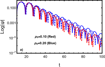
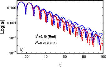
Figure 6: Logarithmic plot of the evolution of a scalar field in Schwdm BH for the case of $l=1$ mode. a) the plot correspond to $\epsilon=0.1$ and b) the plot correspond to $\rho_{0}=0.1$. In both graphs, the solid line is for $\omega_{0}=-1/2$, while the dotted line is for $\omega_{0}=-2/3$.

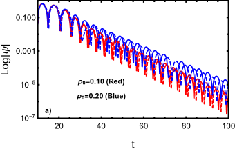
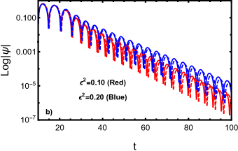
Figure 7: Logarithmic plot of the evolution of a electromagnetic field in Schwdm BH for the case of $l=2$ mode. a) the plot correspond to $\epsilon=0.1$ and b) the plot correspond to $\rho_{0}=0.1$. In both graphs, the solid line is for $\omega_{0}=-1/2$, while the dotted line is for $\omega_{0}=-2/3$.

Fig. 6 demonstrates the evolution of scalar field around of the Schwdm BH with different $\rho_{0}$, $\epsilon^{2}$ and $\omega_{0}$, and in the Fig. 6 the evolution of electromagnetic field is showed.

One can see from Fig. 6 and Fig. 7 that difference of the temporal evolution of the perturbations in the Schwdm BH, is that increases the frequencies of oscillation in the case of the electromagnetic perturbation. Also, it is possible to notice that to $\omega_{0}=-1/2$ and $\omega_{0}=-2/3$ of the Schwdm BH, the evolution of the perturbations are almost the same. Moreover, time domain profiles of the scalar y electromagnetic perturbations of the black hole show that it is stable against perturbations.

VI Conclusions

In this contribution, we have focused on scalar and electromagnetic perturbations of spherically symmetric Schwarzchild black hole with quintessence-like matter and a deficit solid angle. First, we numerically calculated the real and imaginary frequencies of the QNMs. Secondly, we studied the time evaluation of scalar and electromagnetic perturbations.

We calculated the QNMs of Schwdm BH, we apply mainly the Asymptotic Improved Method and WKB approximation sixth order in order, to make a comparison between both methods. The magnitudes of the real part and of the imaginary part of the QNMs for scalar and electromagnetic perturbations decrease with the decreases of values of the density of quintessence-like matter and deficit solid angle. The frequencies are approximately the same and it does not change drastically when the WKB or the AIM methods are considered, so the AIM method is very reliable.

From Tables 1-4, we can see that the change with respect to $\omega_{0}$ of the real part and the magnitude of the imaginary part of the frequencies is very small, while the real part increase with increasing $l$ and the increase of the magnitude of imaginary part of the frequencies is very small.

The evolution of scalar and electromagnetic perturbations obtained in this work confirms that in the QNM stage, all the fields decay slowly due to the presence of quintessence-like matter. At late times, the frequencies are suppressed by the tail form of field decay.

We also saw the behavior of perturbations with changing parameter $\rho_{0}$, $\epsilon^{2}$ and $\omega_{0}$. We note that perturbations with the higher value of $\rho_{0}$ becomes unstable. The behavior of the perturbation for different values of the $\epsilon^{2}$ and $\omega_{0}$ is also studied and reported.

*

Appendix A Improved AIM

In this appendix we briefly explain the improved AIM method. We shall start with the second-order differential equation for the function $\chi(\xi)$

$$\chi^{\prime\prime}=\lambda_{0}(\xi)\chi^{\prime}+s_{0}(\xi)\chi\,.$$ (37)

We can express higher derivatives of $\chi(\xi)$ in terms of $\chi^{\prime}(\xi)$ and $\chi(\xi)$, as following

$$\chi^{(n+2)}=\lambda_{n}(\xi)\chi^{\prime}+s_{n}(\xi)\chi\,,$$ (38)

where

$$\lambda_{n}(\xi) = \lambda^{\prime}_{n-1}(\xi)+s_{n-1}(\xi)+\lambda_{0}(\xi)\lambda_{n-1}(\xi)\,,$$ (39)

$$s_{n}(\xi) = s^{\prime}_{n-1}(\xi)+s_{0}(\xi)\lambda_{n-1}(\xi)\,.$$ (40)

For sufficiently large $n$, the coefficients $\lambda_{n}(\xi)$ and $s_{n}(\xi)$ satisfy the quantization relation

$$s_{n}\lambda_{n-1}-s_{n-1}\lambda_{n}=0\,.$$ (41)

Now, expand the $\lambda_{n}(\xi)$ and $s_{n}(\xi)$ in a Taylor series around the point $\xi_{0}$, we have

$$\lambda_{n}(\xi) = \sum_{i=0}^{\infty}c_{n}^{i}\left(\xi-\xi_{0}\right)^{i}\,,$$ (42)

$$s_{n}(\xi) = \sum_{i=0}^{\infty}d_{n}^{i}\left(\xi-\xi_{0}\right)^{i}\,,$$ (43)

where $c_{n}^{i}$ and $d_{n}^{i}$ are the $i$th Taylor coefficients. Substituting (42) and (43) in (39) and (40), we have the following recursion relations for the coefficients

$$c_{n}^{i} = (i+1)c_{n-1}^{i+1}+d_{n-1}^{i}+\sum_{j=0}^{i}c_{0}^{j}c_{n-1}^{i-j}\,,$$ (44)

$$d_{n}^{i} = (i+1)d_{n-1}^{i+1}+\sum_{j=0}^{i}d_{0}^{j}c_{n-1}^{i-j}\,,$$ (45)

then, the quantization condition (41) can be rewritten as

$$d_{n}^{0}c_{n-1}^{0}-d_{n-1}^{0}c_{n}^{0}=0\,.$$ (46)

Using the quantization condition (46) we can obtain QNMs, for $n$ large enough.

References

- [1] Sai Iyer. BLACK HOLE NORMAL MODES: A WKB APPROACH. 2. SCHWARZSCHILD BLACK HOLES. Phys. Rev. D, 35:3632, 1987.
- [2] Kai Lin, Jin Li, and Shuzheng Yang. Quasinormal Modes of Hayward Regular Black Hole. Int. J. Theor. Phys., 52:3771–3778, 2013.
- [3] Sharmanthie Fernando and Juan Correa. Quasinormal Modes of Bardeen Black Hole: Scalar Perturbations. Phys. Rev. D, 86:064039, 2012.
- [4] Chong Oh Lee, Jin Young Kim, and Mu-In Park. Quasi-normal modes and stability of Einstein–Born–Infeld black holes in de Sitter space. Eur. Phys. J. C, 80(8):763, 2020.
- [5] L. A. López and Valeria Ramírez. Quasi-normal modes of a Generic-class of magnetically charged regular black hole: scalar and electromagnetic perturbations. Eur. Phys. J. Plus, 138(2):120, 2023.
- [6] Omar Pedraza, L. A. López, R. Arceo, and I. Cabrera-Munguia. Quasinormal modes of the Hayward black hole surrounded by quintessence: Scalar, electromagnetic and gravitational perturbations. Mod. Phys. Lett. A, 37(09):2250057, 2022.
- [7] Y. Zhang and Y. X. Gui. Quasinormal modes of a Schwarzschild black hole surrounded by quintessence. Class. Quant. Grav., 23:6141–6147, 2006.
- [8] Mahamat Saleh, Bouetou Thomas Bouetou, and Timoleon Crepin Kofane. Quasinormal modes and Hawking radiation of a Reissner-Nordstroem black hole surrounded by quintessence. Astrophys. Space Sci., 333:449–455, 2011.
- [9] V. V. Kiselev. Quintessence and black holes. Class. Quant. Grav., 20:1187–1198, 2003.
- [10] Chengye Yu, Deyou Chen, and Chuanhong Gao. Quasinormal modes and the correspondence with shadow in black holes with a deficit solid angle and quintessence-like matter. Nucl. Phys. B, 983:115925, 2022.
- [11] Hakan Ciftci, Richard L Hall, and Nasser Saad. Asymptotic iteration method for eigenvalue problems. Journal of Physics A: Mathematical and General, 36(47):11807, nov 2003.
- [12] H. T. Cho, A. S. Cornell, Jason Doukas, T. R. Huang, and Wade Naylor. A New Approach to Black Hole Quasinormal Modes: A Review of the Asymptotic Iteration Method. Adv. Math. Phys., 2012:281705, 2012.
- [13] Manuel Barriola and Alexander Vilenkin. Gravitational Field of a Global Monopole. Phys. Rev. Lett., 63:341, 1989.
- [14] Peng Liu, Chao Niu, and Cheng-Yong Zhang. Instability of regularized 4D charged Einstein-Gauss-Bonnet de-Sitter black holes. Chin. Phys. C, 45(2):025104, 2021.
- [15] Ping Xi, Xi-chen Ao, and Xin-zhou Li. A Simple derivation of level spacing of quasinormal frequencies for a black hole with a deficit solid angle and quintessence-like matter. Astrophys. Space Sci., 330:273–278, 2010.
- [16] Chun-Yan Wang, Ya-Feng Zhao, and Ya-Jun Gao. Quasinormal Modes of a Black Hole with Quintessence-Like Matter and a Deficit Solid Angle for Electromagnetic Perturbation. Commun. Theor. Phys., 57(6):1101–1104, 2012.
- [17] K. A. Bronnikov, R. A. Konoplya, and A. Zhidenko. Instabilities of wormholes and regular black holes supported by a phantom scalar field. Phys. Rev. D, 86:024028, Jul 2012.
- [18] H. T. Cho, A. S. Cornell, Jason Doukas, and Wade Naylor. Black hole quasinormal modes using the asymptotic iteration method. Class. Quant. Grav., 27:155004, 2010.
- [19] Carsten Gundlach, Richard H. Price, and Jorge Pullin. Late time behavior of stellar collapse and explosions: 1. Linearized perturbations. Phys. Rev. D, 49:883–889, 1994.