Calibration in Deep Learning: A Survey of the State-of-the-Art

Abstract

Calibrating deep neural models plays an important role in building reliable, robust AI systems in safety-critical applications. Recent work has shown that modern neural networks that possess high predictive capability are poorly calibrated and produce unreliable model predictions. Though deep learning models achieve remarkable performance on various benchmarks, the study of model calibration and reliability is relatively underexplored. Ideal deep models should have not only high predictive performance but also be well calibrated. There have been some recent advances in calibrating deep models. In this survey, we review the state-of-the-art calibration methods and their principles for performing model calibration. First, we start with the definition of model calibration and explain the root causes of model miscalibration. Then we introduce the key metrics that can measure this aspect. It is followed by a summary of calibration methods that we roughly classify into four categories: post-hoc calibration, regularization methods, uncertainty estimation, and composition methods. We also cover recent advancements in calibrating large models, particularly large language models (LLMs). Finally, we discuss some open issues, challenges, and potential directions.

1 Introduction

Deep Neural Networks (DNNs) have been showing promising predictive power in many domains such as computer vision (?), speech recognition (?) and natural language processing (?). Nowadays, deep neural network models are frequently being deployed into real-world systems. However, recent work (?) pointed out that those highly accurate, negative-log-likelihood (NLL) trained deep neural networks are poorly calibrated (?), i.e., the model predicted class probabilities do not faithfully estimate the true correctness likelihood and lead to overconfident and underconfident predictions. Deploying uncalibrated models into real-world systems is at high risk, particularly for safety-critical applications such as medical diagnosis (?), autonomous driving (?) and finance decision-making.

(a)

(b)

(c)

(d)

Figure 1: An illustration of model calibration. Uncalibrated model (left) that trained with standard cross-entropy loss and calibrated model (right) that trained with focal loss ($\gamma=5$), have similar predictive performance on a binary classification task (accuracy is 83.8% and 83.4% respectively), but the right one is better calibrated. Top: The reliability diagram plots with 10 bins. The diagonal dash line presents perfect calibration (on a specific bin, confidence is equal to accuracy.), Expected Calibration Error (ECE) and Maximum Calibration Error (MCE) are used to measure model calibration performance. Bottom: the posterior distribution of the two models on 1000 samples, the one from calibrated model is better distributed.

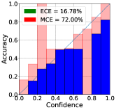
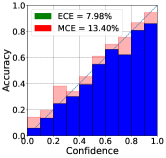
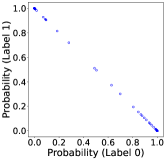
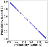
Calibrating deep models is a procedure for preventing the model’s posterior distribution from being over- or under-confident. Figure 1 gives an illustration of calibrating a binary classification model. It is noted that (1) a highly predictive model can be poorly calibrated, this is exhibited by high calibration errors; (2) The deep models tend to be primarily overconfident, this is shown by a spiking posterior distribution.  (?, ?, ?). Model overconfidence is usually caused by over-parameterized networks, a lack of appropriate regularization, limited data, imbalanced label distributions, etc. In the past years, different streams of work have been proposed to calibrate models. In this survey, we review, classify, and discuss recent calibration methods and their advantages and limitations.

1.0.1 Scope and Focus

This survey particularly focuses on calibration methods for classification problems. There have been some related surveys on this topic (?) or on the highly relevant topic–uncertainty estimation. For example model calibration has been briefly discussed in the uncerainty estimation surveys (?, ?). Our survey distinguishes itself from those surveys in several aspects:

• This survey reviews the state-of-the-art calibration methods and focuses mostly on the ones proposed in the last five years. This includes such as kernel-based methods, differentiable calibration proxy, and meta-learning-based approaches. Those are rarely discussed in previous surveys.

• This survey tries to explain calibration principles of each method via the discussion of the conceptual relationships among over-parameterization, over-fitting, and over-confidence. We systematically categorize those methods into post-hoc, regularization (explicit, implicit and differentiable calibration proxy), uncertainty estimation, and composition methods.

• This survey also discusses the methods of calibrating large pre-trained models, particularly large language models (LLMs), where calibrating LLMs in zero-shot inference has been attracting increasing interest from AI communities.

The rest of this survey is structured as follows. In section 2 we introduce the definition of model calibration and discuss the reasons cause miscalibration; Section 2.3 lists the mainstream calibration metrics that are used for measuring model calibration. Section 3 review, classify and discuss recently proposed calibration methods. Section 4 discusses future directions and concludes this survey.

2 Preliminaries and Backgrounds

This section describes the definition of model calibration and the aspects cause miscalibration.

2.1 Definitions

In classification tasks, for a given input variable $X$ and a categorical variable $Y\in\{1,2,...,k\}$, assume we have a neural network model $f$ which maps input variable $\mathbf{x}$ to a categorical distribution $p=\{p_{1},...,p_{k}\}$ over $k$ classes $\{y_{1},...,y_{k}\}$: $f:D\rightarrow\Delta$, where $\Delta$ is the $k-1$ dimensional standard probability simplex and $\Delta=\{p\in[0,1]^{k}|\sum_{i=1}^{k}p_{i}=1\}$. Calibration measures the degree of the match between predicted probability $p$ and the true correctness likelihood. A model $f$ is perfectly calibrated on if and only if:

$$\mathbb{P}(Y=y_{i}|f(X)=p)=p_{i}$$ (1)

where $p$ is true correctness likelihood. Intuitively, for all input pairs $\{x,y\}\in D$, if model predicts $p_{i}=0.8$, we expect that 80% have $y_{i}$ as label.

Instead of probability distribution, the argmax calibration (?, ?, ?) takes only the maximum probability into consideration:

$$\mathbb{P}(Y\in\arg\max(p)|\max(f(X))=p^{*})=p^{*}$$ (2)

In reality, it is difficult to obtain perfect calibration, any deviation from it represents miscalibration.

2.2 Aspects Impact Model Calibration

It has been obversed that some recent changes in modern neural networks are responsible for model miscalibration (?, ?, ?). The underlying general cause is that modern neural networks’ high capacity makes them vulnerable to miscalibration, which is tightly correlated to the concepts of over-parameter, overfitting and over-confidence.

2.2.1 Model Size

While increasing the depth and width of neural networks helps to obtain highly predictive power, it also negatively increases calibration errors. Empirical evidence has shown that this poor calibration is linked to overfitting on the negative log-likelihood (NLL) (?, ?). The over-parameteriaztion is one of the main causes of overfitting. Concretely, along with the standard NLL-based model training, when classification error is minimized, keeping training will further push the model to minimize NLL on the training data, i.e., push the predicted softmax probability distribution as close as possible to the ground-truth distribution (which is usually one-hot). Model overfitting starts by exhibiting increased test NLL, and then the model becomes overconfident (?). For more recent large models, this trend is negligible for in-distribution data and reverses under distribution shift (?).

2.2.2 Regularization

Regularization can effectively prevent overfitting when model capacity increases. Recent trends suggest that explicit L2 regularization may not be necessary to achieve a highly accurate model when applying batch normalization (?) or dropout (?), but Guo et al. (?) emprically demonstrated model tends to be less calibrated without using L2 regularization. There have been more recent regularization techniques  (?, ?, ?, ?) been proposed to improve model calibration.

2.2.3 Data Issues

Another important aspect that impacts calibration is data quantity (e.g., scale, volume, diversity, etc.) and quality (relevance, consistency, completeness, etc.). Training high-capacity (over-parameterized) networks with scarce data can easily cause overfitting and an overconfident model. Data augmentation is an effective way to alleviate this phenomenon and brings implicit calibration effects (?, ?). The recent pretrain-finetune paradigm offers the possibility of reducing overfitting caused by limited and noisy data (?). Another challenge is data imbalance, where models overfit to the majority classes, thus making overconfident predictions for the majority classes. Focal loss (?, ?)  has recently demonstrated promising performance in calibrating deep models.

2.3 Calibration Measurements

Exact calibration measurement with finite data samples is impossible given that the confidence $p$ is a continuous variable (?). There are some popular metrics that approximate model calibration error by grouping $N$ predictions into $M$ interval bins $\{b_{1},b_{2},...,b_{M}\}$.

2.3.1 Expected Calibration Error (ECE)

ECE (?) is a scalar summary statistic of calibration. It is a weighted average of the difference between model accuracy and confidence across $M$ bins,

$$\textsc{ECE}=\frac{1}{N}\sum_{m=1}^{M}\left|b_{m}\right||\textrm{acc}(b_{m})-\textrm{conf}(b_{m})|$$ (3)

where $N$ is the total number of samples. $\left|b_{m}\right|$ is the number of samples in bin $b_{m}$, and

$$\textrm{acc}(b_{m})=\frac{1}{\left|b_{m}\right|}\sum_{i\in B_{m}}\mathbf{1}(\hat{y}_{i}=y_{i}),~{}\textrm{conf}(b_{m})=\frac{1}{\left|b_{m}\right|}\sum_{i\in B_{m}}p_{i}.$$ (4)

2.3.2 Maximum Calibration Error (MCE)

MCE (?) measures the worst-case deviation between accuracy and confidence,

$$\textsc{MCE}=\max_{m\in\{1,\dots,M\}}|\textrm{acc}(b_{m})-\textrm{conf}(b_{m})|.$$ (5)

and is particularly important in high-risk applications where reliable confidence measures are absolutely necessary.

2.3.3 Classwise ECE (CECE)

Classwise ECE (?) can be seen as the macro-averaged ECE. It extends the bin-based ECE to measure calibration across all the possible $K$ classes. In practice, predictions are binned separately for each class, and the calibration error is computed at the level of individual class-bins and then averaged. The metric can be formulated as

$$\textsc{CECE}=\sum_{m=1}^{M}\sum_{c=1}^{K}\frac{|b_{m,c}|}{NK}|\textrm{acc}_{c}(b_{m,c})-\textrm{conf}_{c}(b_{m,c})|$$ (6)

where $b_{m,c}$ represents a single bin for class $c$. In this formulation, $\textrm{acc}_{c}(b_{m,c})$ represents average binary accuracy for class $c$ over bin $b_{m,c}$ and $\textrm{conf}_{c}(b_{m,c})$ represents average confidence for class $c$ over bin $b_{m,c}$.

2.3.4 Adaptive ECE (AECE)

The binning mechanism in the aforementioned metrics can introduce bias; the pre-defined bin size determines the number of samples in each bin. Adaptive ECE (?) introduces a new binning strategy to use an adaptive scheme that spaces the bin intervals to ensure each bin hosts an equal number of samples.

$$\textsc{AECE}=\sum_{r=1}^{R}\sum_{c=1}^{K}\frac{1}{RK}|\textrm{acc}_{c}(b_{n,c})-\textrm{conf}_{c}(b_{n,c})|$$ (7)

Where $r\in[1,R]$ is defined by the $[N/R]$-th index of the sorted and threshold predictions.

For a perfectly calibrated classifier, those calibration erros should equal $0$.

2.3.5 Reliability Diagram

Besides the metrics that provide a scalar summary on calibration, reliability diagrams (as shown in 1) visualize whether a model is over- or under-confident on bins by grouping predictions into bins according to their prediction probability. The diagonal line in Figure 1 presents perfect calibration: $\textrm{acc}(b_{m})=\textrm{conf}(b_{m}),\forall m$, the red bar presents the gap to perfect calibration.

Methods	Categorization	Measurement
Dirichlet Calibration (?)	Post-hoc	CECE, NLL
ATS (?)	Post-hoc	ECE, NLL
BTS (?)	Post-hoc	ECE
LTS (?)	Post-hoc	ECE,MCE,AECE, SCE
Focal Loss  (?)	Reg.(Implicit)	ECE, NLL
FLSD (?)	Reg.(Implicit)	ECE,MCE,AECE, CECE, NLL
MMCE (?)	Reg.(Proxy)	ECE, Brier, NLL
Meta-Calibration (?)	Reg.(Proxy)	ECE
Label Smoothing (?)	Reg.(Aug.)	ECE
Mix-Up (?)	Reg.(Aug.)	ECE
Mix-n-Match (?)	Composition	ECE
TS+MC dropout (?)	Composition	ECE, UCE

Table 1: The state-of-the-art calibration methods and their categorization. The regularization methods are further divided into explicit, implicit regularization and trainable calibration proxies. Uncertainty estimation and quantification methods are excluded, please refer to surveys (?, ?).

3 Calibration Methods

In this section, we categorize the state-of-the-art calibration methods into post-hoc methods, regularization methods, implicit calibration methods, and uncertainty estimation methods. Besides, we discuss compositional methods that combine different calibration methods. Table 1 summarizes those methods.

3.1 Post-hoc Methods

Post-hoc calibration methods aim to calibrate a model after training. Those include non-parametric calibration histogram binning(?), isotonic regression (?) and parametric methods such as Bayesian binning into quantiles (BBQ) and Platt scaling (?). Out of them, Platt scaling (?) based approaches are more popular due to their low complexity and efficiency. This includes Temperature Scaling (TS), attended TS (?).

3.1.1 Temperature Scaling

Temperature scaling (TS) is a single-parameter extension of Platt scaling (?) and the most recent addition to the offering of post-hoc methods. It uses a temperature parameter $\tau$ to calibrate the softmax probability:

$$p_{i}=\frac{\exp(g_{i}/\tau)}{\sum_{j=1}^{k}\exp(g_{j}/\tau)},~{}~{}i\in[1\dots k].$$ (8)

where $\tau>0$ for all classes is used as a scaling factor to soften model predicted probability, it controls the model’s confidence by adjusting the sharpness of distribution so that the model prediction is not too certain (overconfident) or too uncertain (underconfident). The optimal temperature value is obtained by minimizing negative log likelihood loss (NLL) on the validation dataset.:

$$\tau^{\ast}=\arg\min_{\tau}\left(-\sum_{i=1}^{N}\log(\textsc{softmax}(g_{i},\tau)) \right)$$ (9)

TS simplifies matrix (vector) scaling (?) where class-wise $\tau$ is considered as a single parameter, and offers good calibration while maintaining minimum computational complexity (?, ?).

3.1.2 Temperature Scaling Extensions

The goal of post-hoc calibration on a validation dataset is to learn a calibration map (also known as the canonical calibration function of probablity (?)) which transforms uncalibrated probabilities into calibrated ones. Many TS extensions aim to find a proper calibration map.   Kull et al. (?) proposed Dirichlet calibration which assumes probability distributions are parameterized Dirichlet distributions:

$$p(x)|y=j\sim Dirichlet(\alpha^{j})$$ (10)

where $\alpha^{j}=\{\alpha^{j}_{1},\alpha^{j}_{2},...,\alpha^{j}_{k}\}$ are Dirichlet parameters for $j$-th class. The proposed Dirichlet calibration map family coincides with the Beta calibration family (?). Besides, it provides uniqueness and interpretability as compared to generic canonical parametrization.    (?) suggested that TS has difficulties in finding optimal $\tau$ when the validation set has a limited number of samples. They proposed attended temperature scaling (ATS) to alleviate this issue by increasing the number of samples in validation set. The key idea is to gather samples from each class distribution. Let’s assume $p(y|x)$ is the predicted probability. ATS first divides the validation set into $K$ subsets with $p(y=k|x),k\in[1,K]$, which allows to add more $y\neq k$ samples using the Bayeisan Theorem (?) as the selection criterion:

$$p(x,y=k)=\frac{p(y=k|x)}{p(y\neq k|x)}p(x,y\neq k)$$ (11)

It indicates that ATS selects the samples with $y\neq k$ which are more probable to belong to $p(x,y=k)$.   Bin-wise TS (BTS) (?) was proposed to extend TS to multiple equal size bins by using the confidence interval-based binning method. Together with data augmentation, BTS showed superior performance as compared to TS. Local TS (LTS) (?) extends TS to multi-label semantic segmentation and makes it adaptive to local image changes. A local scaling factor is learned for each pixel or voxel.

$$\mathbb{Q}(x,\tau_{i}(x))=max_{l\in L}\textsc{Softmax}(\frac{g_{i}(x)}{\tau_{i}(x)})^{(l)}$$ (12)

where $l$ is the class index, $g_{i}(x)$ is the logit of input at location $x$, and The $\tau_{i}(x)$ is the location-dependent temperature.

Remarks: Although using a single global hyper-parameter, TS remains a popular approach due to its effectiveness and accuracy-preserving (?). Post-hoc calibration usually works well without a huge amount of validation data and is thus data efficient. The calibration procedure is decoupled from training and does not introduce training complexity. On the other hand, post-hoc calibration is less expressive and suffers difficulty in approximating the canonical calibration function when data is not enough (?).

3.2 Regularization Method

Regularization is important to prevent neural network models from overfitting. In this section, we discuss some representative work in this direction that either explicitly or implicitly regularizes modern neural networks to have better calibration.

3.2.1 Explicit Regularization

The typical (explicit) way to add regularization term (or penalty) $L_{reg}$ to standard loss objective (e.g., negative log likelihood):

$$\mathcal{L}(\theta)=-\sum\log p(y|x)+\alpha L_{reg}.$$ (13)

where $\alpha$ controls the importance of penalty in regularizing weight $\theta$. L2 regularization has been widely used in training modern neural networks and showed its effectiveness in model calibration ](?). Entropy regularization (?):

$$\mathcal{L}(\theta)=-\sum\log p(y|x)-\alpha H(p(y|x)).$$ (14)

directly penalizes predictive distributions that have low entropy, prevents these peaked distributions, and ensures better model generalization.

3.2.2 Implicit Regularization: Focal Loss and Its Extensions

Focal loss (?) was originally proposed to alleviate the class imbalance issue in object detection:$\mathcal{L}_{f}=-\sum_{i=1}^{N}(1-p_{i})^{\gamma}\log p_{i}$ where $\gamma$ is a hyperparameter. It has been recently shown that focal loss can be interpreted as a trade-off between minimizing Kullback–Leibler (KL) divergence and maximizing the entropy, depending on $\gamma$ (?):

$$\mathcal{L}_{f}\geq\textsc{KL}(q\parallel p)+\mathbb{H}(q)-\gamma\mathbb{H}(p)$$ (15)

The first term pushes the model to learn a probability $p$ to have a high value (confident, as close as possible to ground-truth label distribution, which is usually one-hot representation). The second term is constant. The last term regularizes probability to not be too high (overconfident).   Mukhoti et al. (?) empirically observed that $\gamma$ plays an important role in implicitly regularizing entropy and weights. However, finding an appropriate $\gamma$ is challenging for all samples in the datasets. Thus, they proposed sample-dependent scheduled $\gamma$ (FLSD) based on the Lambert-W function (?). They have shown that scheduling $\gamma$ values according to different confidence ranges helps to improve model calibration on both in-domain and out-of-domain (OOD) data. More recent extensions focus on computer vision have been proposed, including in margin-based label smoothing (MbLS) (?) and multi-class difference of confidence and accuracy (MDCA) (?).

Differentiable Calibration Proxy: Recall that the aforementioned methods use a penalty term (either explicitly or implicitly) to improve model calibration on dataset $D$. There is a rising direction that directly optimizes objective function by using calibration errors (CE) as differentiable proxy  (?, ?) to standard loss:

$$\arg\min_{\theta}L_{standard}(D,\theta)+L_{calibration}(D,\theta)$$ (16)

The focus of this line of work is to find differentiable approximations to calibration errors.   Kumar et al.  (?) proposed a kernel-based approach to explicitly calibrate models in training phrase called Maximum Mean Calibration Error (MMCE), which is differentiable and can be optimized using batch stochastic gradient algorithms. They cast the calibration error to be differentiable by defining an integral probability measure over functions from a reproducing kernel Hilbert space (RKHS) $\mathcal{H}$ induced by a universal kernel $k(\cdot,\cdot)$ and cannonical feature map $\phi:[0,1]\rightarrow\mathcal{H}$:

$$\textsc{MMCE}(P(r,c))=\left\|E_{(r,c)\sim P}[(c-r)\phi(r)]\right\|_{\mathcal{H}}$$ (17)

where $r,c$ represent confidence and correctness scores, respectively, and $P(r,c)$ denotes the distribution over $r,c$ of the predicted probability $P(y|x)$.   An approach that combines meta-learning and a differentiable calibration proxy was proposed by (?). The authors developed a differentiable ECE(DECE) and used it as learning objective for a meta network. The meta network takes representations from original backbone network and outputs a unit-wise L2 weight decay coefficient $\omega$ for backbone network. The DECE is optimized against calibration metrics with validation set but attached to standard cross-entropy (CE) loss.

$$\omega^{*} =\arg\min_{\omega}\mathcal{L}_{DECE}^{val}(f_{c}^{*}\circ f_{\theta}^{*}(\omega))$$ (18)

$$f_{c}^{*},f_{\theta}^{*}(\omega) =\arg\min_{f_{c},f_{\theta}(\omega)}(\mathcal{L}_{CE}^{train}(f_{c}\circ f_{\theta}(\omega)+\omega\left\|f_{c}\right\|^{2})$$ (19)

where $f_{c}$ is classification layer and $f_{\theta}$ is the feature extractor.

Remarks: Regularization methods, as compared to post-hoc methods, can directly output a well-calibrated model without additional steps. The increased complexity is different for different methods; for instance, focal loss can be seen as an implicit regularization and does not introduce observable additional computational complexity. Kernel-based and meta-network regularization add additional computations depending on the designed kernel methods and meta-networks.

3.3 Data Augmentation

This line of work is highly relevant to regularization methods, instead of directly adding penalty terms to optimization objectives. Those studies try to augment data or add noise to training samples to mitigate model miscalibration. Label smoothing (?) and mixup (?) are popular approaches in this line.   Label smoothing (?) soften hard labels with an introduced smoothing parameter $\alpha$ in the standard loss function (e.g., cross-entropy):

$$\mathcal{L}_{c}=-\sum_{k=1}^{K}y_{k}^{s}\log p_{i},~{}~{}y_{k}^{s}=y_{k}(1-\alpha)+\alpha/K$$ (20)

where $y_{k}$ is the soft label for $k$-th category. It is shown that LS encourages the differences between the logits of the correct class and the logits of the incorrect class to be a constant depending on $\alpha$. The confidence penalty can be recovered by assuming the prior label distribution is a uniform distribution $u$ and reversing the direction of the KL divergence.

$$\mathcal{L}(\theta)=-\sum\log p(y|x)-\textsc{KL}(u\parallel p(y|x)).$$ (21)

Mixup training (?) is another work in this line of exploration. It studies the effectiveness of mixup (?) with respect to model calibration (?). Mixup generates synthetic samples during training by convexly combining random pairs of inputs and labels as well. To mix up two random samples $(x_{i},y_{i})$ and $(x_{j},y_{j})$, the following rules are used:

$$\bar{x} =\alpha x_{i}+(1-\alpha)x_{j}$$ (22)

$$\bar{y} =\alpha y_{i}+(1-\alpha)y_{j}$$ (23)

where $(\bar{x}_{i},\bar{y}_{i})$ is the virtual feature-target of original pairs. The authors observed that mixup-trained models are better calibrated and less prone to overconfidence in prediction on out-of-distribution and noise data. It is pointed out that mixing features alone does not bring calibration benefits; label smoothing can significantly improve calibration when used together with mixing features.

Remarks: This line of work combats overfitting by data augmentation in hidden space. This improves not only model generalization but also calibration. Those methods don’t significantly increase network complexity but usually require more training time due to more generated or synthesized training samples.

3.4 Uncertainty Estimation

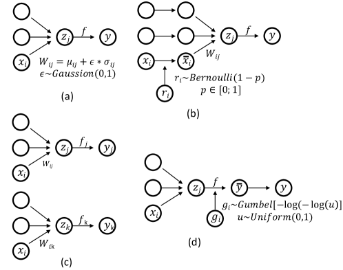
This line of work aims to alleviate model miscalibration by injecting randomness.The popular methods are (1) Bayesian neural networks (?, ?), (2) ensembles (?), (3) Monte Carlo(MC) dropout (?) and (4) Gumbel-softmax (?) based approaches (?, ?). The former three sub-categorgies have been discussed in recent surveys (?, ?)

Figure 2: The methods of uncertainty estimation (?). (a) Bayesian neural network; (b) MC dropout; (c) Ensembles; (d) Gumbel-Softmax trick.

(a)

(b)

(c)

Figure 3: The reliability diagrams for a model trained on CIFAR100 with different bin numbers (left to right: 20, 50, 100). The diagonal dash presents perfect calibration, the red bar presents the gap to perfect calibration on each bin.The calibration error is sensitive to increasing bin numbers.

3.4.1 Bayesian Neural Network

Given a learning objective is to minimize negative log likelihood, $\mathcal{L}=-\frac{1}{N}\sum_{i}^{N}\log p(y_{i}|x_{i},w)$. The probability distribution is obtained by Softmax function as:

$$p(y_{i}=m|x_{i},w)=\frac{\exp(f_{m}(x_{i},w))}{\sum_{k\in M}\exp(f_{k}(x_{i},w)}.$$ (24)

In the inference phase, given a test sample $x^{*}$, the predictive probability $y^{*}$ is computed by:

$$p(y^{*}|x^{*},D)=\int p(y^{*}|x^{*},w)p(w|D)dw$$ (25)

As posterior $p(w|D)$ is intractable, we perform approximation by minimizing the Kullback-Leilber (KL) distance. This can also be treated as the maximization of ELBO:

$$\mathcal{L_{\theta}}=\int q_{\theta}(w)p(Y|X,w)dw-\textsc{KL}[q_{\theta}(w)\parallel p(w)]$$ (26)

where $\theta$ are the variational parameters. With the re-parametrization trick (?), a differentiable mini-batched Monte Carlo (MC) estimator can be obtained.

The uncertainty estimation can be done by performing $T$ inference runs and averaging predictions: $p(y*|x*)=\frac{1}{T}\sum_{t=1}^{T}p_{w_{t}}(y^{*}|x^{*},w_{t}).$

3.4.2 MC Dropout, Ensembles and Gumbel-Softmax

By following the above-mentioned strategy, MC-dropout (?), ensembles (?) and Gumbel-softmax sampling (?, ?) introduce randomness in different ways, as illustrated in Figure 2. Then the $T$ in equation (29) corresponds to the number of sets of mask vectors from Bernoulli distribution $\{r^{t}\}_{t=1}^{T}$ in MC-dropout, or the number of randomly trained models in Ensembles, which potentially leads to different sets of learned parameters $\omega=\{\omega_{1},...,\omega_{t}\}$, or the number of sets of sampled attention distribution from Gumbel distribution $\{g^{t}\}_{t=1}^{T}$.

Remarks: This line of work requires multiple inference runs to perform approximations. This increases computational overhead significantly as compared to previous methods. On the other hand, besides model calibration, those methods are primarily proposed for uncertainty quantification and estimation. Therefore, network uncertainty can be captured and measured as well.

3.5 Composition Calibration

Beside applying each method independently, we can always have calibration compositions by combining two or more methods. One straightforward way to combine non-post-hoc methods with post-hoc methods. For instance, performing Temperature Scaling (TS) after employing the regularization method and implicit calibration (?, ?). Thulasidasan et al. (?) observed that the combination of label smoothing and mixup training significantly improved calibration. While there are several possibilities for combining different approaches, we highlight some interesting compositions.

3.5.1 Ensemble Temperature Scaling (ETS)

Zhang et al. (?) gave three important definitions related to calibration properties: accuracy-preserving, data-efficient, and expressive. They pointed out that TS is an accuracy-preserving and data-efficient approach but is less expressive. Ensemble Temperature Scaling (ETS) was proposed to improve TS expressivity while maintaining the other two properties:

$$T(z;w,\tau)=w_{1}T(z;\tau)+w_{2}z+w_{3}K^{-1}$$ (27)

There are three ensemble components: the original TS $T(z;\tau)=(z_{1}^{\tau^{-1}},...,z_{k}^{\tau^{-1}})/\sum_{k=1}^{K}z_{k}^{\tau^{-1}}$, uncalibrated prediction with $\tau=1$ and uniform prediction for each class $z_{k}=K^{-1}$.

3.5.2 Temperature Scaling with MC Dropout

Laves et al. (?) extended TS to dropout variational inference to calibrate model uncertainty. The key idea is to insert $\tau$ before final softmax activation and insert TS with $\tau>0$ before softmax activation in MC integration:$\hat{p}=\frac{1}{N}\sum_{i=1}^{N}\textsc{softmax}(\frac{f_{w_{i}}(x)}{\tau})$ where $N$ forward passes are performed to optimize $\tau$ with respect to NLL on the validation set. Then the entropy of the softmax likelihood is used to represent the uncertainty of all $C$ classes.

$$H(p)=-\frac{1}{\log C}\sum p^{c}\log p^{c},H\in[0,1]$$ (28)

Remarks: Appropriately combining different calibration types to some degree can further improve calibration, but, it may also combine their disadvantages, for instance, Ensemble Temperature Scaling (ETS) (?) has increased complexity.

3.6 Calibrating Pre-trained Large Models

Pre-trained large models, including vision, language, or vision-language models, have been increasingly used in many safety-critical and customer-facing applications. The calibration of those large models has been recently studied and revisited (?, ?).

3.6.1 Large Vision Model Calibration

Minderer et al. (?) studied recent state-of-the-art vision models that include vision transformer (?) and MLP-mixer (?). They found out that the model size and amount of pre-training in the recent model generation could not fully explain the observed decay of calibration with distribution shift or model size in the prior model generation. They also discussed the correlation between in-distribution and out-of-distribution (OOD) calibration. They pointed out that the models with better in-distribution calibration also gave better calibration on OOD benchmarks. LeVine et al. (?) studied the calibration of CLIP (?) as a zero-shot inference model and found that CLIP is miscalibrated in zero-shot settings.They showed effectiveness of learning a temperature on an auxiliary task and applying it to inference regardless of prompt or datasets.

3.6.2 Large Language Models (LLMs)

The LLMs and prompting engineering have become an efficient learning paradigm and can perform numerous natural language tasks without or with only few examples. However, the outcome of this learning paradigm can be unstable and introduces bias with various prompt templates and training examples (?). The introduced biases include majority label bias, recency bias and token bias. To mitigate this bias, Zhao et al. (?) proposed contextual calibration procedure to improve the predictive power of GPT-3 on few-shot learning tasks with a context-free input such as ”N/A”. The contextual calibration is performed by using vector scaling (?).

Similarly, Zheng et al. (?) investaged the selection bais of LLMs in multi-choice question (MCQ) task and pinpointed that LLMs’ token bias is an intrinsic cause of the selection bias. They proposed

Park et al. (?) extended mixup (?) training to improve model calibration by synthesizing samples based on the Area Under the Margin (AUM) for pre-trained language models.   Prototypical calibration (PROCA)  (?) is one of the latest studies in calibrating LLMs. It showed the importance of decision boundary in few-shot classification settings and suggested learning a better boundary with a prototypical cluster. Concretely, it estimates $K$ category-wise clusters with the Gaussian mixture model (GMM):

$$P_{GMM}(x)=\sum_{k=1}^{K}\alpha_{k}p_{G}(x|u_{k},\Sigma_{k})$$ (29)

where $u_{k}$ and $\Sigma_{k}$ are the mean vector and covariance matrix of the distribution. The parameters $\{\alpha,u,\Sigma\}_{k=1}^{K}$ are estimated by using the Expectation-Maximization (EM) algorithm (?) with a small unlabelled dataset.

4 Conclusion and Future Work

We have reviewed the state-of-the-art calibration methods, described with the motivations, causes, measurement metrics, and categorizations. Then we discussed the details and principles of recent methods as well as their individual advantages and disadvantages. Despite recent advances in calibrating deep models, there are still some challenges and underexplored aspects and needs further exploration.

4.1 Mitigating Calibration Bias

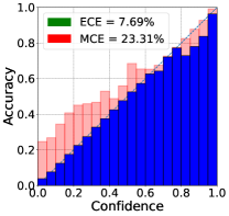
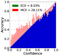
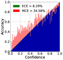
Accurately and reliably measuring calibration is still challenging due to the introduced biases from the binning mechanism and the finite sample numbers (?). For the former challenge, it mainly suffers from sensitivity and data inefficiency issues. The sensitivity to the binning scheme is presented in 3. We can see that for a given model, increasing bin numbers gives higher ECE and MCE scores. A KDE-based ECE Estimator (?) was proposed to replace histograms with non-parametric density estimators, which are continuous and more data-efficient. Measuring the bias is then important for having a correct calibration evaluation. Roelofs et al. (?) proposed Bias-by-Construction (BBC) to model the bias in bin-based ECE as a function of the number of samples and bins. It confirms the existence of non-negligible statistical biases. To follow this line of work, future efforts will include developing an unbiased calibration estimator, exploring the trade-off between calibration bias and variance as mentioned in  (?).

4.2 Calibrating Generative Models

Most recent calibration efforts have focused on classification and regression tasks; model calibration for sequence generation is rarely discussed in the literature. Kumar et al. (?) pointed out the token-level probability in neural machine translation tasks is poorly calibrated, which explains the counter-intuitive BLEU drop with increased beam-size (?). The token-level probability miscalibration is further confirmed in LLM for few-shot learning (?). The main cause is the softmax bottleneck (?) on large vocabulary. In the task of sequence generation, early token probability miscalibration can magnify the entire sequence. How to effectively calibrate token-level probability in various settings would be an interesting direction, particularly in the era of LLMs.

References

- Blundell et al. Blundell, C., Cornebise, J., Kavukcuoglu, K., & Wierstra, D. (2015). Weight uncertainty in neural network. In International conference on machine learning, pp. 1613–1622. PMLR.
- Bohdal et al. Bohdal, O., Yang, Y., & Hospedales, T. (2021). Meta-calibration: Meta-learning of model calibration using differentiable expected calibration error. arXiv preprint arXiv:2106.09613.
- Bojarski et al. Bojarski, M., Del Testa, D., Dworakowski, D., Firner, B., Flepp, B., Goyal, P., Jackel, L. D., Monfort, M., Muller, U., Zhang, J., et al. (2016). End to end learning for self-driving cars. arXiv preprint arXiv:1604.07316.
- Caruana et al. Caruana, R., Lou, Y., Gehrke, J., Koch, P., Sturm, M., & Elhadad, N. (2015). Intelligible models for healthcare: Predicting pneumonia risk and hospital 30-day readmission. In Proceedings of the 21th ACM SIGKDD international conference on knowledge discovery and data mining, pp. 1721–1730.
- Corless et al. Corless, R. M., Gonnet, G. H., Hare, D. E., Jeffrey, D. J., & Knuth, D. E. (1996). On the lambertw function. Advances in Computational mathematics, 5(1), 329–359.
- Desai & Durrett Desai, S., & Durrett, G. (2020). Calibration of pre-trained transformers. In EMNLP, pp. 295–302.
- Ding et al. Ding, Z., Han, X., Liu, P., & Niethammer, M. (2021). Local temperature scaling for probability calibration. In Proceedings of the IEEE/CVF International Conference on Computer Vision, pp. 6889–6899.
- Dosovitskiy et al. Dosovitskiy, A., Beyer, L., Kolesnikov, A., Weissenborn, D., Zhai, X., Unterthiner, T., Dehghani, M., Minderer, M., Heigold, G., Gelly, S., et al. An image is worth 16x16 words: Transformers for image recognition at scale. In International Conference on Learning Representations.
- Fortunato et al. Fortunato, M., Blundell, C., & Vinyals, O. (2017). Bayesian recurrent neural networks. arXiv preprint arXiv:1704.02798.
- Gal & Ghahramani Gal, Y., & Ghahramani, Z. (2016). Dropout as a bayesian approximation: Representing model uncertainty in deep learning. In ICML’16, pp. 1050–1059. PMLR.
- Gawlikowski et al. Gawlikowski, J., Tassi, C. R. N., Ali, M., Lee, J., Humt, M., Feng, J., Kruspe, A., Triebel, R., Jung, P., Roscher, R., et al. (2021). A survey of uncertainty in deep neural networks. arXiv preprint arXiv:2107.03342.
- Graves et al. Graves, A., Mohamed, A.-r., & Hinton, G. (2013). Speech recognition with deep recurrent neural networks. In 2013 IEEE international conference on acoustics, speech and signal processing, pp. 6645–6649. Ieee.
- Guo et al. Guo, C., Pleiss, G., Sun, Y., & Weinberger, K. Q. (2017). On calibration of modern neural networks. In ICML, pp. 1321–1330. PMLR.
- Han et al. Han, Z., Hao, Y., Dong, L., Sun, Y., & Wei, F. (2023). Prototypical calibration for few-shot learning of language models. In The Eleventh International Conference on Learning Representations.
- Hebbalaguppe et al. Hebbalaguppe, R., Prakash, J., Madan, N., & Arora, C. (2022). A stitch in time saves nine: A train-time regularizing loss for improved neural network calibration. In Proceedings of the IEEE/CVF Conference on Computer Vision and Pattern Recognition, pp. 16081–16090.
- Ioffe & Szegedy Ioffe, S., & Szegedy, C. (2015). Batch normalization: Accelerating deep network training by reducing internal covariate shift. In International conference on machine learning, pp. 448–456. pmlr.
- Jang et al. Jang, E., Gu, S., & Poole, B. (2017). Categorical reparameterization with gumbel-softmax. In ICLR’17.
- Ji et al. Ji, B., Jung, H., Yoon, J., Kim, K., et al. (2019). Bin-wise temperature scaling (bts): Improvement in confidence calibration performance through simple scaling techniques. In 2019 IEEE/CVF International Conference on Computer Vision Workshop (ICCVW), pp. 4190–4196. IEEE.
- Jin et al. Jin, L., Lazarow, J., & Tu, Z. (2017). Introspective classification with convolutional nets. NeurIPS, 30.
- Kingma et al. Kingma, D. P., Salimans, T., & Welling, M. (2015). Variational dropout and the local reparameterization trick. In NeurIPS’15, Vol. 28, pp. 2575–2583.
- Koehn & Knowles Koehn, P., & Knowles, R. (2017). Six challenges for neural machine translation. In First Workshop on Neural Machine Translation, pp. 28–39. Association for Computational Linguistics.
- Krizhevsky et al. Krizhevsky, A., Sutskever, I., & Hinton, G. E. (2012). Imagenet classification with deep convolutional neural networks. NeurIPS, 25.
- Kull et al. Kull, M., Filho, T. S., & Flach, P. (2017). Beta calibration: a well-founded and easily implemented improvement on logistic calibration for binary classifiers. In Proceedings of the 20th International Conference on Artificial Intelligence and Statistics, Vol. 54, pp. 623–631. PMLR.
- Kull et al. Kull, M., Perello Nieto, M., Kängsepp, M., Silva Filho, T., Song, H., & Flach, P. (2019). Beyond temperature scaling: Obtaining well-calibrated multi-class probabilities with dirichlet calibration. NeurIPS, 32.
- Kumar & Sarawagi Kumar, A., & Sarawagi, S. (2019). Calibration of encoder decoder models for neural machine translation. arXiv preprint arXiv:1903.00802.
- Kumar et al. Kumar, A., Sarawagi, S., & Jain, U. (2018). Trainable calibration measures for neural networks from kernel mean embeddings. In ICML, pp. 2805–2814. PMLR.
- Lakshminarayanan et al. Lakshminarayanan, B., Pritzel, A., & Blundell, C. (2017). Simple and scalable predictive uncertainty estimation using deep ensembles. In NeurIPS’17.
- Laves et al. Laves, M.-H., Ihler, S., Kortmann, K.-P., & Ortmaier, T. (2019). Well-calibrated model uncertainty with temperature scaling for dropout variational inference. arXiv preprint arXiv:1909.13550.
- LeVine et al. LeVine, W., Pikus, B., Raj, P., & Gil, F. A. (2023). Enabling calibration in the zero-shot inference of large vision-language models. arXiv preprint arXiv:2303.12748.
- Lin et al. Lin, T.-Y., Goyal, P., Girshick, R., He, K., & Dollár, P. (2017). Focal loss for dense object detection. In Proceedings of the IEEE international conference on computer vision, pp. 2980–2988.
- Liu et al. Liu, B., Ben Ayed, I., Galdran, A., & Dolz, J. (2022). The devil is in the margin: Margin-based label smoothing for network calibration. In Proceedings of the IEEE/CVF Conference on Computer Vision and Pattern Recognition, pp. 80–88.
- Mena et al. Mena, J., Pujol, O., & Vitria, J. (2021). A survey on uncertainty estimation in deep learning classification systems from a bayesian perspective. ACM Computing Surveys (CSUR), 54(9), 1–35.
- Minderer et al. Minderer, M., Djolonga, J., Romijnders, R., Hubis, F., Zhai, X., Houlsby, N., Tran, D., & Lucic, M. (2021a). Revisiting the calibration of modern neural networks. NeurIPS, 34.
- Minderer et al. Minderer, M., Djolonga, J., Romijnders, R., Hubis, F., Zhai, X., Houlsby, N., Tran, D., & Lucic, M. (2021b). Revisiting the calibration of modern neural networks..
- Moon Moon, T. K. (1996). The expectation-maximization algorithm. IEEE Signal processing magazine, 13(6), 47–60.
- Mozafari et al. Mozafari, A. S., Gomes, H. S., Leão, W., Janny, S., & Gagné, C. (2018). Attended temperature scaling: a practical approach for calibrating deep neural networks. arXiv preprint arXiv:1810.11586.
- Mukhoti et al. Mukhoti, J., Kulharia, V., Sanyal, A., Golodetz, S., Torr, P., & Dokania, P. (2020). Calibrating deep neural networks using focal loss. NeurIPS, 33, 15288–15299.
- Müller et al. Müller, R., Kornblith, S., & Hinton, G. E. (2019). When does label smoothing help?. NeurIPS, 32.
- Naeini et al. Naeini, M. P., Cooper, G. F., & Hauskrecht, M. (2015). Obtaining well calibrated probabilities using bayesian binning. In Proceedings of the Twenty-Ninth AAAI Conference on Artificial Intelligence (AAAI).
- Niculescu-Mizil & Caruana Niculescu-Mizil, A., & Caruana, R. (2005). Predicting good probabilities with supervised learning. In ICML, pp. 625–632.
- Nixon et al. Nixon, J., Dusenberry, M. W., Zhang, L., Jerfel, G., & Tran, D. (2019). Measuring calibration in deep learning.. In CVPR Workshops, Vol. 2.
- Park & Caragea Park, S. Y., & Caragea, C. (2022). On the calibration of pre-trained language models using mixup guided by area under the margin and saliency. In Proceedings of the 60th Annual Meeting of the Association for Computational Linguistics (Volume 1: Long Papers), pp. 5364–5374.
- Pei et al. Pei, J., Wang, C., & Szarvas, G. (2022). Transformer uncertainty estimation with hierarchical stochastic attention. In AAAI, Vol. 36, pp. 11147–11155.
- Pereyra et al. Pereyra, G., Tucker, G., Chorowski, J., Kaiser, Ł., & Hinton, G. (2017). Regularizing neural networks by penalizing confident output distributions. arXiv preprint arXiv:1701.06548.
- Platt et al. Platt, J., et al. (1999). Probabilistic outputs for support vector machines and comparisons to regularized likelihood methods. Advances in large margin classifiers, 10(3), 61–74.
- Radford et al. Radford, A., Kim, J. W., Hallacy, C., Ramesh, A., Goh, G., Agarwal, S., Sastry, G., Askell, A., Mishkin, P., Clark, J., et al. (2021). Learning transferable visual models from natural language supervision. In International conference on machine learning, pp. 8748–8763. PMLR.
- Roelofs et al. Roelofs, R., Cain, N., Shlens, J., & Mozer, M. C. (2022). Mitigating bias in calibration error estimation. In International Conference on Artificial Intelligence and Statistics, pp. 4036–4054. PMLR.
- Silva Filho et al. Silva Filho, T., Song, H., Perello-Nieto, M., Santos-Rodriguez, R., Kull, M., & Flach, P. (2023). Classifier calibration: a survey on how to assess and improve predicted class probabilities. Machine Learning, 1–50.
- Srivastava et al. Srivastava, N., Hinton, G., Krizhevsky, A., Sutskever, I., & Salakhutdinov, R. (2014). Dropout: a simple way to prevent neural networks from overfitting. The journal of machine learning research, 15(1), 1929–1958.
- Thulasidasan et al. Thulasidasan, S., Chennupati, G., Bilmes, J. A., Bhattacharya, T., & Michalak, S. (2019). On mixup training: Improved calibration and predictive uncertainty for deep neural networks. NeurIPS, 32.
- Tolstikhin et al. Tolstikhin, I. O., Houlsby, N., Kolesnikov, A., Beyer, L., Zhai, X., Unterthiner, T., Yung, J., Steiner, A., Keysers, D., Uszkoreit, J., et al. (2021). Mlp-mixer: An all-mlp architecture for vision. NeurIPS, 34, 24261–24272.
- Vaicenavicius et al. Vaicenavicius, J., Widmann, D., Andersson, C., Lindsten, F., Roll, J., & Schön, T. (2019). Evaluating model calibration in classification. In The 22nd International Conference on Artificial Intelligence and Statistics, pp. 3459–3467. PMLR.
- Vaswani et al. Vaswani, A., Shazeer, N., Parmar, N., Uszkoreit, J., Jones, L., Gomez, A. N., Kaiser, Ł., & Polosukhin, I. (2017). Attention is all you need. NeurIPS, 30.
- Wang et al. Wang, C., Lawrence, C., & Niepert, M. (2021a). Uncertainty estimation and calibration with finite-state probabilistic rnns. In ICLR’21.
- Wang et al. Wang, D.-B., Feng, L., & Zhang, M.-L. (2021b). Rethinking calibration of deep neural networks: Do not be afraid of overconfidence. NeurIPS, 34, 11809–11820.
- Yang et al. Yang, Z., Dai, Z., Salakhutdinov, R., & Cohen, W. W. (2018). Breaking the softmax bottleneck: A high-rank rnn language model. In International Conference on Learning Representations.
- Zadrozny & Elkan Zadrozny, B., & Elkan, C. (2001). Obtaining calibrated probability estimates from decision trees and naive bayesian classifiers. In Icml, Vol. 1, pp. 609–616. Citeseer.
- Zadrozny & Elkan Zadrozny, B., & Elkan, C. (2002). Transforming classifier scores into accurate multiclass probability estimates. In Proceedings of the eighth ACM SIGKDD international conference on Knowledge discovery and data mining, pp. 694–699.
- Zhang et al. Zhang, H., Cisse, M., Dauphin, Y. N., & Lopez-Paz, D. (2018). mixup: Beyond empirical risk minimization. In International Conference on Learning Representations.
- Zhang et al. Zhang, J., Kailkhura, B., & Han, T. Y.-J. (2020). Mix-n-match: Ensemble and compositional methods for uncertainty calibration in deep learning. In ICML, pp. 11117–11128. PMLR.
- Zhang et al. Zhang, L., Deng, Z., Kawaguchi, K., & Zou, J. (2022). When and how mixup improves calibration. In International Conference on Machine Learning, pp. 26135–26160. PMLR.
- Zhao et al. Zhao, Z., Wallace, E., Feng, S., Klein, D., & Singh, S. (2021). Calibrate before use: Improving few-shot performance of language models. In ICML, pp. 12697–12706. PMLR.
- Zheng et al. Zheng, C., Zhou, H., Meng, F., Zhou, J., & Huang, M. (2023). On large language models’ selection bias in multi-choice questions. arXiv preprint arXiv:2309.03882.