Model Selection for Exposure-Mediator Interaction
For the Alzheimer’s Disease Neuroimaging Initiative

Abstract

In mediation analysis, the exposure often influences the mediating effect, i.e., there is an interaction between exposure and mediator on the dependent variable. When the mediator is high-dimensional, it is necessary to identify non-zero mediators (M) and exposure-by-mediator (X-by-M) interactions. Although several high-dimensional mediation methods can naturally handle X-by-M interactions, research is scarce in preserving the underlying hierarchical structure between the main effects and the interactions. To fill the knowledge gap, we develop the XMInt procedure to select M and X-by-M interactions in the high-dimensional mediators setting while preserving the hierarchical structure. Our proposed method employs a sequential regularization-based forward-selection approach to identify the mediators and their hierarchically preserved interaction with exposure. Our numerical experiments showed promising selection results. Further, we applied our method to ADNI morphological data and examined the role of cortical thickness and subcortical volumes on the effect of amyloid-beta accumulation on cognitive performance, which could be helpful in understanding the brain compensation mechanism.

Keywords Brain compensation  $\cdot$ Exposure by mediator interaction  $\cdot$ Hierarchical structure  $\cdot$ High-dimensional mediators  $\cdot$ Model selection  $\cdot$ Mediation analysis  $\cdot$ Neuroimaging

1 Introduction

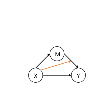
Figure 1: A graphical representation of the mediation effect of the intervening variable M on the relationship between the independent variable X and the dependent variable Y (black arrows, upper triangular part) and the interaction effect between X and M (orange arrow)

A mediation model examines how an independent variable or an exposure (X) affects a dependent variable (Y) through one or more intervening variables or mediators (M) (Baron and Kenny, 1986; Robins and Greenland, 1992; Holland, 1988; MacKinnon, 2008; Sobel, 2008; Preacher and Hayes, 2008; Imai et al., 2010; Vanderweele, 2011; Imai and Yamamoto, 2013; Pearl, 2013; VanderWeele and Vansteelandt, 2014; VanderWeele, 2015; Daniel et al., 2015). In the mediation mechanism, we often observe that X influences the mediating effect of M on Y, i.e., there is an interaction between X and M on the dependent variable (Y), as represented in Figure 1.

In the single mediator case, VanderWeele (2014) proposed the 4-way decomposition method to handle the X-by-M interaction, which was used in Wang et al. (2019) to find the mediated interaction effect. This decomposition idea was later extended to the few mediators case, such as in VanderWeele and Vansteelandt (2014) and Bellavia and Valeri (2018).

New mediation methods have also been developed to address the issue of high dimensions in the mediators. Some used regularization-based methods (Zhao and Luo, 2016; Serang et al., 2017; Li et al., 2021). Others used hybrid methods such as the combined filter method with coordinate descent algorithm (van Kesteren and Oberski, 2019), screening and regularization (Zhang et al., 2016, 2021; Luo et al., 2020; Schaid and Sinnwell, 2020), and dimension reduction and regularization (Zhao et al., 2020).

For models involving interactions with high-dimensional data, it is important to preserve the underlying hierarchical structure between the main effects and the interactions (Hao and Zhang, 2017; Nelder, 1977). In regression settings, regularization methods with different penalty functions (Efron et al., 2004; Yuan et al., 2009; Zhao et al., 2009; Choi et al., 2010; Bien et al., 2013) have been developed to aid the interaction selection, but they become infeasible as the number of independent variables increases (Hao et al., 2018). To address such limitation, Hao et al. (2018) proposed an efficient interaction selection method for high-dimensional data, the regularization algorithm under marginality principle (RAMP), in which possible interaction terms are sequentially added based on the current main effects.

Compared to the regression settings, it is more challenging to preserve the hierarchical structure between the main effects and interactions in the mediation analysis because model selection now involves two models: M on X and Y on M. Although the high-dimensional mediation methods mentioned earlier may naturally handle X-by-M interactions, research is scarce in preserving such hierarchy. Therefore, in this paper, we aim to identify the mediators and the exposure by mediator interactions in the high-dimensional mediators setting while addressing the underlying hierarchical structure between the main effects and interactions.

This identification of mediators and their hierarchically preserved interaction with exposure can be useful in explaining how the brain reacts during the process of brain-related changes and in understanding the brain compensation mechanism, defined as the phenomenon that the effect of the brain on the outcome is altered. For example, under the context of cognitive aging and brain pathology, where we have cognitive or clinical performance as the outcome, aging or pathology as the exposure, and certain brain measures such as cortical thickness as the potential mediators, we often observe that thinner cortical thickness (M) is associated with the worse cognitive performance (Y), and further, in the presence of some pathology (X), we observe the opposite association or no association anymore. In other words, the brain acts differently on the outcome because of the exposure (i.e., there is X-by-M interaction), which illustrates the brain compensation mechanism based on our definition. Or alternatively, we may think that the brain tries to compensate for the loss in cognition due to the pathology, which is also indicative of the idea of compensation.

Our proposed method employs a sequential regularization-based forward-selection approach to identify the mediators and their interactions with exposure while preserving the hierarchical structure between them. We will sequentially update the selected mediator and interaction set (initially empty) based on the selection in the previous step. For example, if a mediator is identified but its corresponding interaction term is not, we will include the identified mediator into the selected mediator set in the next step while keeping the selected interaction set as it is; if both the mediator and its corresponding interaction are identified, we will include them into the selected mediator set and the selected interaction set, respectively; if an interaction is identified, but its involving M is not, we will not only include the interaction into the selected interaction set but also include the involving M into the mediator set to preserve the hierarchical structure. Recently, Wang et al. (2020) proposed a method designed specifically for high-dimensional compositional microbiome mediators, in which the selection of the interaction between treatment and mediators was considered. In contrast to their method, our method focuses on the continuous mediators, which do not have any sum constraint on the mediators as in the microbiome data. In addition, instead of adding overall penalties to the objective function to preserve the hierarchical structure as in Wang et al. (2020), we adopt an adaptive way to update the penalties and include the potential mediator if either its interaction with the exposure is selected or its main effect is selected in the previous step.

In this paper, we first introduced our proposed algorithm in Section 2. Then, we presented the simulation results in Section 3. Finally, we applied our method to the real-world human brain imaging data and examined the role of cortical thickness and subcortical volumes on the relationship between amyloid beta accumulation and cognitive performance in Section 4.

2 Methods

We aim to identify the mediators (M) and their interactions with exposure (X) while preserving the hierarchical structure between the main effects and interaction effects. The multivariate mediation model that we consider takes the following form. For each subject $i=1,...,n$,

$$\mathbf{M}_{i}=\bm{a_{0}}+\bm{a}X_{i}+{\bm{e_{1}}}_{i},$$

$$Y_{i}=c_{0}+cX_{i}+\mathbf{M}_{i}^{\top}\bm{b_{1}}+(X_{i}\times\mathbf{M}_{i}^{\top})\ \bm{b_{2}}+e_{2_{i}},$$

where $\mathbf{M}_{i}=(M_{i,1}\ \cdots\ M_{i,V})^{\top}$, $\bm{a_{0}}=(a_{0_{1}}\ \cdots\ a_{0_{V}})^{\top}$, $\bm{a}=(a_{1}\ \cdots\ a_{V})^{\top}$, $\mathbf{e_{1}}_{i}=(e_{1_{i,1}}\ \cdots\ e_{1_{i,V}})^{\top}$ $\sim{MVN}(\mathbf{0},\Sigma)$, $\bm{b_{1}}=(b_{1_{1}}\ \cdots\ b_{1_{V}})^{\top}$, $\bm{b_{2}}=(b_{2_{1}}\ \cdots\ b_{2_{V}})^{\top}$, and $e_{2_{i}}\sim N(0,\sigma^{2})$.

$X$ is the independent variable or the exposure of interest, $Y$ is the dependent variable or the outcome of interest, and $M_{v}$’s, where $v=1,...,V$, are the variables that might have the potential to mediate the effect of $X$ on $Y$. $X\times M_{v}$ interaction terms are included to investigate whether $X$ changes the way how $M_{v}$ affects $Y$. Any $M_{v}$ with non-zero $a_{v}$ and $b_{1_{v}}$ coefficients is considered to be a mediator. Any $X\times M_{v}$ with non-zero $b_{2_{v}}$ coefficient is considered to have an interaction effect.

The joint distribution of the outcome and the mediator can be written as $f_{Y,M\mid\cdot}(y,m\mid\cdot)=f_{Y\mid M,\cdot}(y\mid m,\cdot)\ f_{M\mid\cdot}(m\mid\cdot).$ Under the Gaussian assumption of the error terms, the log-likelihood is given as

$$\ell({\bm{\theta}}) = \sum_{i=1}^{n}\ell_{Y,\mathbf{M}\mid\bm{\theta}}(\bm{\theta}\mid Y_{i},\mathbf{M}_{i})=\sum_{i=1}^{n}\ell_{Y\mid\mathbf{M},\bm{\theta}}(\bm{\theta}\mid Y_{i},\mathbf{M}_{i})+\sum_{i=1}^{n}\ell_{\mathbf{M}\mid\bm{\theta}}(\bm{\theta}\mid\mathbf{M}_{i})$$

$$= -n\log(2\pi)-\frac{n}{2}\log\sigma^{2}+\frac{n}{2}\log\mid\Omega\mid$$

$$-\frac{1}{2\sigma^{2}}\sum_{i=1}^{n}\Big{(}Y_{i}-c_{0}-cX_{i}-\mathbf{M}_{i}^{\top}\bm{b_{1}}-(X_{i}\times\mathbf{M}_{i}^{\top})\ \bm{b_{2}}\Big{)}^{2}$$

$$-\frac{1}{2}\sum_{i=1}^{n}(\mathbf{M}_{i}-\bm{a_{0}}-\bm{a}X_{i})^{\top}\Omega(\mathbf{M}_{i}-\bm{a_{0}}-\bm{a}X_{i}),$$

where $\Omega=\Sigma^{-1}$.

We denote $\mathcal{M}=\{1,2,...,V\}$ be the index set for all of the $V$ potential mediators $\mathbf{M}$, $\mathcal{M}_{k}$ be the index set for the mediators identified in step $k$, $\mathcal{M}_{k}^{c}=\mathcal{M}-\mathcal{M}_{k}$ be the index set for the remaining M variables (out of $V$ variables), $\mathcal{I}_{k}$ be the index set for the involving M variables in the interaction terms identified in step $k$, and $\mathcal{I}_{k}^{c}=\mathcal{M}-\mathcal{I}_{k}$ be the index set for the involving M variables in remaining interaction terms (out of $V$ variables).

Our algorithm is described as follows. Table 1 provides a summary of the algorithm.

1. Initialization

First, we standardize the data and compute $\lambda_{max}=n^{-1}\max\mid\mathbf{[X\ M\ X\times M]}^{\top}\mathbf{Y}\mid$ and $\lambda_{min}=\zeta\lambda_{max}$ for some small $\zeta>0$ (e.g., 0.05). Based on the determined $\lambda_{max}$ and $\lambda_{min}$, we generate an exponentially decaying sequence with length $K$ (e.g. 20), $\lambda_{max}=\lambda_{1}>\lambda_{2}>\cdots>\lambda_{K}=\lambda_{min}$. Also, we start with $\mathcal{M}_{0}=\emptyset$ and $\mathcal{I}_{0}=\emptyset$.

2. Find regularization path

For each $k=1,...,K$, we minimize the following objective function (2), in the form of negative log-likelihood plus penalties, with respect to $\bm{a,b_{1},b_{2}}$.

$$n\log\sigma^{2} -n\log\mid\Omega\mid+\sum_{i=1}^{n}(\mathbf{M}_{i}-\bm{a_{0}}-\bm{a}X_{i})^{\top}\Omega(\mathbf{M}_{i}-\bm{a_{0}}-\bm{a}X_{i})$$

$$+\frac{1}{\sigma^{2}}\sum_{i=1}^{n}\Big{(}Y_{i}-c_{0}-cX_{i}-\mathbf{M}_{i}^{\top}\bm{b_{1}}-(X_{i}\times\mathbf{M}^{\top}_{i})\bm{b_{2}}\Big{)}^{2}$$

$$+\lambda_{k}\mid\mid\bm{b}_{1_{v\in\mathcal{M}_{k-1}^{c}\cup\mathcal{I}_{k-1}^{c}}}\mid\mid_{1}+\lambda_{k}\mid\mid\bm{b}_{2_{v\in\mathcal{I}_{k-1}^{c}}}\mid\mid_{1}+\lambda_{k}\mid\mid\bm{a}_{v\in\mathcal{M}_{k-1}^{c}\cup\mathcal{I}_{k-1}^{c}}\mid\mid_{1}$$ (1)

The penalization at current step $k$ is imposed based on the selected mediator set and the selected interaction set from the previous step (or, $\mathcal{M}_{k-1}$ and $\mathcal{I}_{k-1}$). If a $M_{v}$ variable is selected as a mediator in the previous step (i.e., the index $v$ is in $\mathcal{M}_{k-1}$), then we will not penalize the corresponding $a_{v}$ and $b_{1_{v}}$ at the current step. If a $X\times M_{v}$ variable is selected as an interaction in the previous step (i.e., the index $v$ is in $\mathcal{I}_{k-1}$), then we will not only not penalize the corresponding $b_{2_{v}}$ but also not penalize the corresponding $a_{v}$ and $b_{1_{v}}$ to force the main effect to be included into the model so that the hierarchical structure is preserved. These altogether form the penalty terms in the objection function (2).

We utilize an iterative estimation approach to estimate the nuisance parameters $\sigma^{2}$ and $\Omega$ using QUIC R package and $\bm{a,b_{1},b_{2}}$ using glmnet R package. We then update the selected mediator set and the selected interaction set correspondingly based on the estimated coefficients. The mediators identified (i.e. the $M_{v}$ variables with non-zero $a_{v}$ and $b_{1_{v}}$ coefficients) at current step $k$ form the current selected mediator set (i.e., their indices $v$’s form $\mathcal{M}_{k}$). The interactions identified (i.e. the $X\times M_{v}$ variables with non-zero $b_{2_{v}}$ coefficient) at current step $k$ form the current selected interaction set (i.e., their indices $v$’s form $\mathcal{I}_{k}$).

3. Model selection

Then, we compute Haughton’s Bayesian information criterion (HBIC; Haughton (1988)) between the current model and the null model. HBIC for two model comparison can be computed as $HBIC=2[\ell({\bm{\hat{\theta_{2}}}})-\ell({\bm{\hat{\theta_{1}}}})]-(d_{2}-d_{1})\log\Big{(}\frac{N}{2\pi}\Big{)},$ where $\ell({\bm{\hat{\theta_{j}}}})$ is the log-likelihood function of the model $j$, $d_{j}$ is the number of parameters of the model $j$, and $N$ is the sample size (Bollen et al., 2014). HBIC is chosen to evaluate the model performance instead of cross-validation because cross-validation may not perform well with a limited sample size. Previous studies have shown that HBIC stands out in the selection of measurement models (Haughton et al., 1997; Lin et al., 2017); among the information criterion (IC) measures, the scaled unit information prior BIC (SPBIC) and the HBIC have the best overall performance in choosing the true full structural models (Bollen et al., 2014; Lin et al., 2017); SPBIC and HBIC performed the best in selecting path models and were recommended for model comparison in structural equation modeling (SEM) (Lin et al., 2017); HBIC might be preferable to SPBIC for its simplicity in computation (Lin et al., 2017). We select the model with the smallest HBIC as the final model.

Note that in the initialization step, $\lambda_{max}$ should be set to ensure that we start with the null model. In occasional cases, the computed $\lambda_{max}$ can be too small to give a null model as the starting point. To account for that, our algorithm gradually enlarges $\lambda_{max}$ by a factor (1.5 by default, which is a 50% increase from the previous one) until we start with a null model.

3 Simulation

For each subject $i=1,\cdots,N$, the exposure $X_{i}$ was independently generated from the standard normal distribution, each potential mediator was independently generated as $M_{i,v}=a_{v}X_{i}+\varepsilon_{1_{i,v}}$, where $\varepsilon_{1_{i,v}}\stackrel{{\scriptstyle i.i.d.}}{{\sim}}\ N(0,1)$, and the outcome $Y_{i}$ was generated as $Y_{i}=1\cdot X_{i}+\Sigma_{v}b_{1_{v}}M_{i,v}+\Sigma_{v}b_{2_{v}}X_{i}\times M_{i,v}+\varepsilon_{2_{i}}$, where $\varepsilon_{2_{i}}\stackrel{{\scriptstyle i.i.d.}}{{\sim}}\ N(0,1)$. We set the first three $M$ variables ($M_{1},M_{2},M_{3}$) to be the true mediators (i.e., having non-zero $a$ and $b_{1}$ coefficients) and set $X\times M_{1}$ to be the true exposure-by-mediator interaction term (i.e., having non-zero $b_{2}$ coefficient).

In this simulation, the sample size was set to be $N=100,200,400$, and the number of potential mediators was set to be $V=50,100,200,400$. The effect size (ES) represents the value of $a,b_{1},b_{2}$ of the truth, which are $a_{1},a_{2},a_{3},b_{1_{1}},b_{1_{2}},b_{1_{3}},b_{2_{1}}$ in our case. We set $ES=0.25,0.5,0.75,1$ and set all other coefficient values to 0. Also, we used the default $K=20$ and $\zeta=0.05$ to generate the $\lambda$ sequence. The final model is given by the $\lambda$ that minimizes HBIC.

Under each simulation scenario, we calculated the average true positive rate (TPR) and the average false discovery rate (FDR) across the 100 simulation runs for the mediator and the interaction, respectively. For each simulation run, the TPR was computed as the proportion of the truth that was selected by the algorithm. For example, the TPR for the mediator is

$${\mbox{TPR}_{\mbox{med}}}=\frac{\mbox{the number of selected true mediators}}{\mbox{the number of true mediators}},$$

and the TPR for the interaction is

$${\mbox{TPR}_{\mbox{int}}}=\frac{\mbox{the number of selected true interactions}}{\mbox{the number of true interactions}}.$$

The FDR was computed as the proportion of the falsely selected non-truth variables from the selection. That is, the FDR for the mediator is

$${\mbox{FDR}_{\mbox{med}}}=\frac{\mbox{the number of falsely selected mediators}}{\mbox{the number of selected mediators}},$$

and the FDR for the interaction is

$${\mbox{FDR}_{\mbox{int}}}=\frac{\mbox{the number of falsely selected interactions}}{\mbox{the number of selected interactions}}.$$

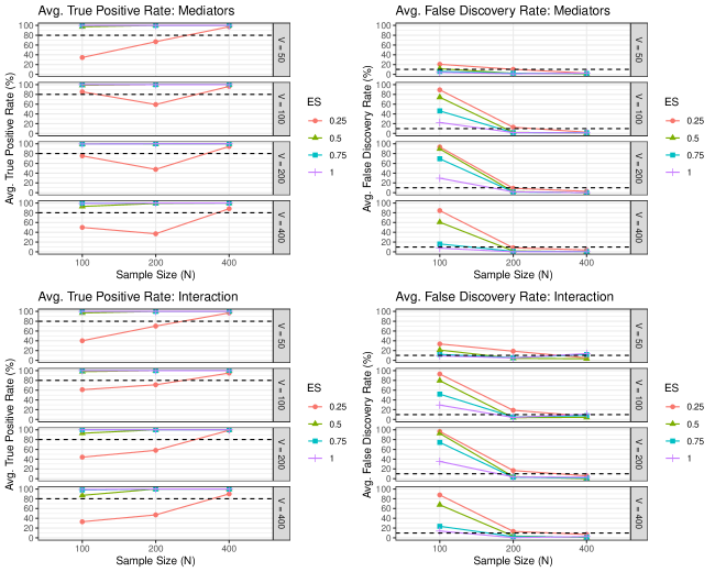
Figure 2: The average True Positive Rate (TPR) and the average False Discovery Rate (FDR) across the 100 simulation runs by the sample size (N), the number of potential mediators (V) and the effect size (ES), for (a) the mediator (upper panel) and for (b) the interaction (lower panel), respectively

Figure 2 shows the average TPR and the average FDR across the 100 simulation runs by the sample size, the number of potential mediators and the effect size, for (a) the mediator and for (b) the interaction, respectively. By the forward-selection feature of our algorithm, the hierarchical structure between interactions and mediators is preserved. Our results show that the average TPR generally increases with effect size, for both the mediator and the interaction. When the effect size and the sample size were moderate to large (N at least 200, ES at least 0.5), our algorithm can almost 100% of the time identify all of the three true mediators and the true interaction term (TPR close to 100%) and it is not likely to falsely select the non-truth (FDRs controlled under approximately 10%). Also, we observed that by increasing the sample size, we may be able to make up for a small effect size to some degree and maintain a reasonably high TPR.

4 Data Application

We applied our algorithm to the human brain imaging data from the Alzheimer’s Disease Neuroimaging Initiative (ADNI), a longitudinal multicenter study designed for the early detection and tracking of Alzheimer’s disease. Specifically, we assessed the role of cortical thickness and subcortical volumes on the relationship between amyloid beta accumulation and cognitive abilities. We used the data from the participants without dementia – diagnosed as mild cognitive impairment (MCI; N = 458) or cognitively normal (CN; N = 276). Participants’ characteristics are displayed in Table 2.

The data were downloaded from the ADNI database (http://adni.loni.usc.edu). The initial phase (ADNI-1) recruited 800 participants, including approximately 200 healthy controls, 400 patients with late MCI, and 200 patients clinically diagnosed with AD over 50 sites across the United States and Canada and followed up at 6- to 12-month intervals for 2–3 years. ADNI has been followed by ADNI-GO and ADNI-2 for existing participants and enrolled additional individuals, including early MCI. To be classified as MCI in ADNI, a subject needed an inclusive Mini-Mental State Examination score of between 24 and 30, subjective memory complaint, objective evidence of impaired memory calculated by scores of the Wechsler Memory Scale Logical Memory II adjusted for education, a score of 0.5 on the Global Clinical Dementia Rating, absence of significant confounding conditions such as current major depression, normal or near-normal daily activities, and absence of clinical dementia.

All studies were approved by their respective institutional review boards and all subjects or their surrogates provided informed consent compliant with HIPAA regulations.

The exposure of interest is amyloid beta accumulation. CSF amyloid beta (A$\beta$-42) concentrations were measured in picograms per milliliter (pg/mL) by ADNI researchers using the highly automated Roche Elecsys immunoassays on the Cobas e601 automated system following extensive validation studies (Bittner et al., 2016; Shaw et al., 2016). The CSF data used in this study were obtained from the ADNI files UPENNBIOMK9_04_19_17.csv. Detailed descriptions of CSF acquisition including lumbar puncture procedures, measurement, and quality control procedures were presented in http://adni.loni.usc.edu/methods/.

The outcome variable of interest is the memory composite score. We used ADNI’s pre-generated cognitive composite scores that were constructed based on bi-factor confirmatory factor analyses models (Crane et al., 2012). Composite memory scores were derived using the Rey Auditory Verbal Learning Test, AD Assessment Schedule-Cognition, Mini-Mental State Examination, and Logical Memory.

MPRAGE T1-weighted MR images were used in this analysis. Cross-sectional image processing was performed using FreeSurfer Version 7.0.1. Region of interest (ROI)-specific cortical thickness and volume measures were extracted from the automated FreeSurfer anatomical parcellation using the Desikan-Killiany Atlas (Desikan et al., 2006) for cortical regions and ASEG (Fischl et al., 2002) for subcortical regions. We considered 89 potential mediators that were derived from 68 cortical thickness measures from both left and right hemispheres, 5 corpus callosum subregion volume measures, and 16 subcortical volume measures from both left and right hemispheres (Thalamus, Caudate, Putamen, Pallidum, Hippocampus, Amygdala, Accumbens, VentralDC). Since the volume measures are typically confounded by brain size, we divided them by the estimated total intracranial volume to adjust for the potential confounding effect. Further, as all these 89 measures are often correlated with sex and age, we regressed them on sex and age and used the residuals as our potential mediators.

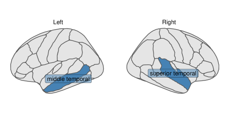
Figure 3: Two cortical thickness measures (one in the middle temporal region in the left hemisphere and the other in the superior temporal region in the right hemisphere) that were identified to have the mediated interaction effects on the relationship between amyloid beta accumulation and memory using XMInt on ADNI dataset

Our algorithm identified mediated interaction effects of cortical thickness from two temporal regions: the middle temporal region in the left hemisphere and the superior temporal region in the right hemisphere, as shown in Figure 3. In other words, the cortical thickness of the two identified regions mediates the relationship between amyloid beta accumulation and cognitive abilities, and further, their effect on cognition is influenced by amyloid beta accumulation. The direction of the interaction can also be explored using the 4-way decomposition idea proposed in VanderWeele (2014) and VanderWeele and Vansteelandt (2014). Under the counterfactual independence assumptions, it showed that when there is no amyloid beta accumulation, the thinner cortex in the middle temporal region of the left hemisphere and the superior temporal region of the right hemisphere is associated with worse cognitive performance (PIE = 0.036, p < 0.01); however, when there is more amyloid beta accumulation involved, such mediation effect disappears – the thinner cortex is no longer associated with worse cognition (TIE = 0.010, p = 0.1). These altogether illustrate the brain compensation mechanism during this process of brain-related changes.

5 Discussion

In this paper, we proposed the XMInt algorithm to identify the mediators and the exposure by mediator interactions in the high-dimensional mediators setting while preserving the underlying hierarchical structure between the main effects and the interaction effects, and we investigated the conditions when our algorithm demonstrates ideal model selection performance. Based on our simulation results, when the effect size and the sample size are moderate to large, our algorithm was able to correctly identify the true mediators and interaction almost all the time, without falsely selecting many non-truth variables. To illustrate our algorithm, we also applied our method to real-world human brain imaging data. Two cortical thickness measures (one in the middle temporal region in the left hemisphere and the other in the superior temporal region in the right hemisphere) were identified to have mediated interaction effects on the relationship between amyloid beta accumulation and memory abilities. This identification of temporal thickness as a mediator is consistent with the existing literature (e.g., Villeneuve et al. (2014)). Further, we found that when there is no amyloid beta accumulation, a thinner cortex in these two identified regions is associated with worse cognitive performance, but when there is more amyloid beta accumulation involved, the mediation effect in these two regions disappears, which helps illustrate the brain compensation mechanism. One limitation is that when the number of potential mediators or the sample size becomes larger, it may take a longer time to run the algorithm, as the estimation of $\Sigma^{-1}$ for the HBIC computation becomes slower. In summary, our algorithm works well and can be used as an effective tool to identify the mediated interaction with preserved hierarchical structure in the mediation analysis.

Software

The XMInt R package is available at https://github.com/ruiyangli1/XMInt, and the package usage with examples is available at https://ruiyangli1.github.io/XMInt/.

Disclosure statement

The authors report there are no competing interests to declare.

Funding

This work was supported by NIH R01AG062578 (PI: Lee). Data collection and sharing for this project was funded by the Alzheimer’s Disease Neuroimaging Initiative (ADNI) (National Institutes of Health Grant U01 AG024904) and DOD ADNI (Department of Defense award number W81XWH-12-2-0012). ADNI is funded by the National Institute on Aging, the National Institute of Biomedical Imaging and Bioengineering, and through generous contributions from the following: AbbVie, Alzheimer’s Association; Alzheimer’s Drug Discovery Foundation; Araclon Biotech; BioClinica, Inc.; Biogen; Bristol-Myers Squibb Company; CereSpir, Inc.; Cogstate; Eisai Inc.; Elan Pharmaceuticals, Inc.; Eli Lilly and Company; EuroImmun; F. Hoffmann-La Roche Ltd and its affiliated company Genentech, Inc.; Fujirebio; GE Healthcare; IXICO Ltd.; Janssen Alzheimer Immunotherapy Research & Development, LLC.; Johnson & Johnson Pharmaceutical Research & Development LLC.; Lumosity; Lundbeck; Merck & Co., Inc.; Meso Scale Diagnostics, LLC.; NeuroRx Research; Neurotrack Technologies; Novartis Pharmaceuticals Corporation; Pfizer Inc.; Piramal Imaging; Servier; Takeda Pharmaceutical Company; and Transition Therapeutics. The Canadian Institutes of Health Research is providing funds to support ADNI clinical sites in Canada. Private sector contributions are facilitated by the Foundation for the National Institutes of Health (www.fnih.org). The grantee organization is the Northern California Institute for Research and Education, and the study is coordinated by the Alzheimer’s Therapeutic Research Institute at the University of Southern California. ADNI data are disseminated by the Laboratory for NeuroImaging at the University of Southern California.

Data availability statement

Data used in preparation of this article were obtained from the Alzheimer’s Disease Neuroimaging Initiative (ADNI) database (adni.loni.usc.edu), under the data use agreement by ADNI. The simulation experiment data example is available at https://ruiyangli1.github.io/XMInt/articles/Simulation.html.

Tables and Figures

Table 1: XMInt Algorithm Summary

Input:	$\mathbf{X}$, $\mathbf{Y}$, potential $\mathbf{M}$
Output:	Selected mediator(s) and exposure by mediator interaction(s)
1. Initialization:	$\bullet$ standardize $\mathbf{X}$, $\mathbf{Y}$, $\mathbf{M}$
	$\bullet$ using standardized data, generate an exponentially decaying sequence
	$\lambda_{max}=\lambda_{1}>\lambda_{2}>\cdots>\lambda_{K}=\lambda_{min}$
	$\circ$ compute $\lambda_{max}=n^{-1}\max\mid\mathbf{[X\ M\ X\times M]}^{\top}\mathbf{Y}\mid$
	$\circ$ set $\lambda_{min}=\zeta\lambda_{max}$ with some small $\zeta>0$
	$\bullet$ $\mathcal{M}_{0}=\emptyset$, $\mathcal{I}_{0}=\emptyset$
2. Find regularization path:	For each $k=1,\cdots,K$,
	$\bullet$ minimize (2) w.r.t $\bm{a,b_{1},b_{2}}$ and get estimation
	- regarding the penalization in (2)
	$\cdot$ If $v\in\mathcal{M}_{k-1}$, then do not penalize $a_{v}$ and $b_{1_{v}}$
	$\cdot$ If $v\in\mathcal{I}_{k-1}$, then do not penalize $a_{v}$, $b_{1_{v}}$ and $b_{2_{v}}$
	$\bullet$ update $\mathcal{M}_{k}$ and $\mathcal{I}_{k}$
	$\circ$ $v$’s with nonzero $a_{v}$ and $b_{1_{v}}$ form $\mathcal{M}_{k}$
	$\circ$ $v$’s with nonzero $b_{2_{v}}$ form $\mathcal{I}_{k}$
	$\bullet$ compute HBIC
3. Model selection:	select the final model with the smallest HBIC

Table 2: Participants’ Characteristics (ADNI Dataset)

Characteristic	Overall, N = 7341	CN, N = 2761	MCI, N = 4581
Abeta accumulation (pg/mL)	1,088.5 (447.3)	1,229.3 (440.6)	1,003.6 (430.1)
Memory composite scores	0.6 (0.7)	1.1 (0.6)	0.3 (0.7)
Age (years)	71.9 (7.0)	72.8 (5.9)	71.4 (7.6)
Sex
Male	381 (51.9%)	121 (43.8%)	260 (56.8%)
Female	353 (48.1%)	155 (56.2%)	198 (43.2%)
Education (years)	16.3 (2.6)	16.5 (2.5)	16.2 (2.7)
Ethnicity
Hispanic	24 (3.3%)	11 (4.0%)	13 (2.8%)
Not Hispanic	706 (96.2%)	262 (94.9%)	444 (96.9%)
Unknown	4 (0.5%)	3 (1.1%)	1 (0.2%)
Race
White	681 (92.8%)	252 (91.3%)	429 (93.7%)
Non-White	51 (6.9%)	24 (8.7%)	27 (5.9%)
Unknown	2 (0.3%)	0 (0.0%)	2 (0.4%)
1n (%); Mean (Standard Deviation)
CN: cognitively normal; MCI: mild cognitive impairment

References

- Baron and Kenny [1986] Reuben M. Baron and David A. Kenny. The moderator–mediator variable distinction in social psychological research: Conceptual, strategic, and statistical considerations. Journal of Personality and Social Psychology, 51(6):1173–1182, 1986. ISSN 1939-1315. doi:10.1037/0022-3514.51.6.1173.
- Robins and Greenland [1992] James M. Robins and Sander Greenland. Identifiability and Exchangeability for Direct and Indirect Effects. Epidemiology, 3(2):143–155, 1992. ISSN 1044-3983. URL http://www.jstor.org/stable/3702894.
- Holland [1988] Paul W. Holland. Causal Inference, Path Analysis, and Recursive Structural Equations Models. Sociological Methodology, 18:449–484, 1988. ISSN 0081-1750. doi:10.2307/271055. URL http://www.jstor.org/stable/271055.
- MacKinnon [2008] David P. MacKinnon. Introduction to Statistical Mediation Analysis. Routledge, New York, January 2008. ISBN 978-0-203-80955-6. doi:10.4324/9780203809556.
- Sobel [2008] Michael E. Sobel. Identification of Causal Parameters in Randomized Studies with Mediating Variables. Journal of Educational and Behavioral Statistics, 33(2):230–251, 2008. ISSN 1076-9986. URL http://www.jstor.org/stable/20172114.
- Preacher and Hayes [2008] Kristopher J. Preacher and Andrew F. Hayes. Asymptotic and resampling strategies for assessing and comparing indirect effects in multiple mediator models. Behavior Research Methods, 40(3):879–891, August 2008. ISSN 1554-3528. doi:10.3758/BRM.40.3.879. URL https://doi.org/10.3758/BRM.40.3.879.
- Imai et al. [2010] Kosuke Imai, Luke Keele, and Teppei Yamamoto. Identification, Inference and Sensitivity Analysis for Causal Mediation Effects. Statistical Science, 25(1):51–71, 2010. ISSN 0883-4237. URL https://www.jstor.org/stable/41058997.
- Vanderweele [2011] Tyler J. Vanderweele. Controlled Direct and Mediated Effects: Definition, Identification and Bounds. Scandinavian Journal of Statistics, 38(3):551–563, 2011. ISSN 1467-9469. doi:10.1111/j.1467-9469.2010.00722.x. URL https://onlinelibrary.wiley.com/doi/abs/10.1111/j.1467-9469.2010.00722.x.
- Imai and Yamamoto [2013] Kosuke Imai and Teppei Yamamoto. Identification and Sensitivity Analysis for Multiple Causal Mechanisms: Revisiting Evidence from Framing Experiments. Political Analysis, 21(2):141–171, 2013. ISSN 1047-1987. URL http://www.jstor.org/stable/24572652.
- Pearl [2013] Judea Pearl. Direct and Indirect Effects. arXiv:1301.2300 [cs, stat], January 2013. URL http://arxiv.org/abs/1301.2300.
- VanderWeele and Vansteelandt [2014] Tyler VanderWeele and Stijn Vansteelandt. Mediation Analysis with Multiple Mediators. Epidemiologic Methods, 2(1):95–115, January 2014. ISSN 2161-962X. doi:10.1515/em-2012-0010. URL https://www.degruyter.com/document/doi/10.1515/em-2012-0010/html.
- VanderWeele [2015] Tyler VanderWeele. Explanation in Causal Inference: Methods for Mediation and Interaction. Oxford University Press, February 2015. ISBN 978-0-19-932588-7.
- Daniel et al. [2015] R. M. Daniel, B. L. De Stavola, S. N. Cousens, and S. Vansteelandt. Causal Mediation Analysis with Multiple Mediators. Biometrics, 71(1):1–14, 2015. ISSN 0006-341X. URL http://www.jstor.org/stable/24538398.
- VanderWeele [2014] Tyler J. VanderWeele. A unification of mediation and interaction: a four-way decomposition. Epidemiology (Cambridge, Mass.), 25(5):749–761, September 2014. ISSN 1044-3983. doi:10.1097/EDE.0000000000000121. URL https://www.ncbi.nlm.nih.gov/pmc/articles/PMC4220271/.
- Wang et al. [2019] Yun Wang, Joel Bernanke, Bradley S. Peterson, Patrick McGrath, Jonathan Stewart, Ying Chen, Seonjoo Lee, Melanie Wall, Vanessa Bastidas, Susie Hong, Bret R. Rutherford, David J. Hellerstein, and Jonathan Posner. The association between antidepressant treatment and brain connectivity in two double-blind, placebo-controlled clinical trials: a treatment mechanism study. The Lancet Psychiatry, 6(8):667–674, August 2019. ISSN 2215-0366, 2215-0374. doi:10.1016/S2215-0366(19)30179-8. URL https://www.thelancet.com/journals/lanpsy/article/PIIS2215-0366(19)30179-8/fulltext.
- Bellavia and Valeri [2018] Andrea Bellavia and Linda Valeri. Decomposition of the Total Effect in the Presence of Multiple Mediators and Interactions. American Journal of Epidemiology, 187(6):1311–1318, June 2018. ISSN 0002-9262. doi:10.1093/aje/kwx355. URL https://doi.org/10.1093/aje/kwx355.
- Zhao and Luo [2016] Yi Zhao and Xi Luo. Pathway Lasso: Estimate and Select Sparse Mediation Pathways with High Dimensional Mediators. arXiv:1603.07749 [stat], March 2016. URL http://arxiv.org/abs/1603.07749.
- Serang et al. [2017] Sarfaraz Serang, Ross Jacobucci, Kim C. Brimhall, and Kevin J. Grimm. Exploratory Mediation Analysis via Regularization. Structural Equation Modeling: A Multidisciplinary Journal, 24(5):733–744, September 2017. ISSN 1070-5511. doi:10.1080/10705511.2017.1311775. URL https://doi.org/10.1080/10705511.2017.1311775.
- Li et al. [2021] Bin Li, Qingzhao Yu, Lu Zhang, and Meichin Hsieh. Regularized multiple mediation analysis. Statistics and Its Interface, 14(4):449–458, 2021. ISSN 1938-7997. doi:10.4310/21-SII664. URL https://www.intlpress.com/site/pub/pages/journals/items/sii/content/vols/0014/0004/a007/abstract.php.
- van Kesteren and Oberski [2019] Erik-Jan van Kesteren and Daniel L. Oberski. Exploratory Mediation Analysis with Many Potential Mediators. Structural Equation Modeling: A Multidisciplinary Journal, 26(5):710–723, September 2019. ISSN 1070-5511. doi:10.1080/10705511.2019.1588124. URL https://doi.org/10.1080/10705511.2019.1588124.
- Zhang et al. [2016] Haixiang Zhang, Yinan Zheng, Zhou Zhang, Tao Gao, Brian Joyce, Grace Yoon, Wei Zhang, Joel Schwartz, Allan Just, Elena Colicino, Pantel Vokonas, Lihui Zhao, Jinchi Lv, Andrea Baccarelli, Lifang Hou, and Lei Liu. Estimating and testing high-dimensional mediation effects in epigenetic studies. Bioinformatics, 32(20):3150–3154, October 2016. ISSN 1367-4803. doi:10.1093/bioinformatics/btw351. URL https://doi.org/10.1093/bioinformatics/btw351.
- Zhang et al. [2021] Haixiang Zhang, Yinan Zheng, Lifang Hou, Cheng Zheng, and Lei Liu. Mediation analysis for survival data with high-dimensional mediators. Bioinformatics, 37(21):3815–3821, November 2021. ISSN 1367-4803. doi:10.1093/bioinformatics/btab564. URL https://doi.org/10.1093/bioinformatics/btab564.
- Luo et al. [2020] Chengwen Luo, Botao Fa, Yuting Yan, Yang Wang, Yiwang Zhou, Yue Zhang, and Zhangsheng Yu. High-dimensional mediation analysis in survival models. PLOS Computational Biology, 16(4):e1007768, April 2020. ISSN 1553-7358. doi:10.1371/journal.pcbi.1007768. URL https://journals.plos.org/ploscompbiol/article?id=10.1371/journal.pcbi.1007768.
- Schaid and Sinnwell [2020] Daniel J. Schaid and Jason P. Sinnwell. Penalized models for analysis of multiple mediators. Genetic Epidemiology, 44(5):408–424, 2020. ISSN 1098-2272. doi:10.1002/gepi.22296. URL http://onlinelibrary.wiley.com/doi/abs/10.1002/gepi.22296.
- Zhao et al. [2020] Yi Zhao, Martin A. Lindquist, and Brian S. Caffo. Sparse principal component based high-dimensional mediation analysis. Computational Statistics & Data Analysis, 142:106835, February 2020. ISSN 0167-9473. doi:10.1016/j.csda.2019.106835. URL https://www.sciencedirect.com/science/article/pii/S0167947319301902.
- Hao and Zhang [2017] Ning Hao and Hao Helen Zhang. A Note on High-Dimensional Linear Regression With Interactions. The American Statistician, 71(4):291–297, October 2017. ISSN 0003-1305. doi:10.1080/00031305.2016.1264311. URL https://doi.org/10.1080/00031305.2016.1264311.
- Nelder [1977] J. A. Nelder. A Reformulation of Linear Models. Journal of the Royal Statistical Society. Series A (General), 140(1):48–77, 1977. ISSN 0035-9238. doi:10.2307/2344517. URL https://www.jstor.org/stable/2344517. Publisher: [Royal Statistical Society, Wiley].
- Efron et al. [2004] Bradley Efron, Trevor Hastie, Iain Johnstone, and Robert Tibshirani. Least Angle Regression. The Annals of Statistics, 32(2), April 2004. ISSN 0090-5364. doi:10.1214/009053604000000067. URL http://arxiv.org/abs/math/0406456.
- Yuan et al. [2009] Ming Yuan, V. Roshan Joseph, and Hui Zou. STRUCTURED VARIABLE SELECTION AND ESTIMATION. The Annals of Applied Statistics, 3(4):1738–1757, 2009. ISSN 1932-6157. URL http://www.jstor.org/stable/27801569.
- Zhao et al. [2009] Peng Zhao, Guilherme Rocha, and Bin Yu. The composite absolute penalties family for grouped and hierarchical variable selection. The Annals of Statistics, 37(6A), December 2009. ISSN 0090-5364. doi:10.1214/07-AOS584. URL http://arxiv.org/abs/0909.0411.
- Choi et al. [2010] Nam Hee Choi, William Li, and Ji Zhu. Variable Selection With the Strong Heredity Constraint and Its Oracle Property. Journal of the American Statistical Association, 105(489):354–364, March 2010. ISSN 0162-1459. doi:10.1198/jasa.2010.tm08281. URL https://doi.org/10.1198/jasa.2010.tm08281.
- Bien et al. [2013] Jacob Bien, Jonathan Taylor, and Robert Tibshirani. A lasso for hierarchical interactions. The Annals of Statistics, 41(3):1111–1141, June 2013. ISSN 0090-5364, 2168-8966. doi:10.1214/13-AOS1096. URL https://projecteuclid.org/journals/annals-of-statistics/volume-41/issue-3/A-lasso-for-hierarchical-interactions/10.1214/13-AOS1096.full.
- Hao et al. [2018] Ning Hao, Yang Feng, and Hao Helen Zhang. Model Selection for High-Dimensional Quadratic Regression via Regularization. Journal of the American Statistical Association, 113(522):615–625, April 2018. ISSN 0162-1459. doi:10.1080/01621459.2016.1264956. URL https://amstat.tandfonline.com/doi/citedby/10.1080/01621459.2016.1264956.
- Wang et al. [2020] Chan Wang, Jiyuan Hu, Martin J Blaser, and Huilin Li. Estimating and testing the microbial causal mediation effect with high-dimensional and compositional microbiome data. Bioinformatics, 36(2):347–355, January 2020. ISSN 1367-4803. doi:10.1093/bioinformatics/btz565. URL https://doi.org/10.1093/bioinformatics/btz565.
- Haughton [1988] Dominique M. A. Haughton. On the Choice of a Model to Fit Data from an Exponential Family. The Annals of Statistics, 16(1):342–355, March 1988. ISSN 0090-5364, 2168-8966. doi:10.1214/aos/1176350709. URL https://projecteuclid.org/journals/annals-of-statistics/volume-16/issue-1/On-the-Choice-of-a-Model-to-Fit-Data-from/10.1214/aos/1176350709.full. Publisher: Institute of Mathematical Statistics.
- Bollen et al. [2014] Kenneth A. Bollen, Jeffrey J. Harden, Surajit Ray, and Jane Zavisca. BIC and Alternative Bayesian Information Criteria in the Selection of Structural Equation Models. Structural Equation Modeling: A Multidisciplinary Journal, 21(1):1–19, January 2014. ISSN 1070-5511. doi:10.1080/10705511.2014.856691. URL https://doi.org/10.1080/10705511.2014.856691. Publisher: Routledge _eprint: https://doi.org/10.1080/10705511.2014.856691.
- Haughton et al. [1997] Dominique M.A. Haughton, Johan H.L. Oud, and Robert A.R.G. Jansen. Information and other criteria in structural equation model selection. Communications in Statistics - Simulation and Computation, 26(4):1477–1516, January 1997. ISSN 0361-0918. doi:10.1080/03610919708813451. URL https://doi.org/10.1080/03610919708813451. Publisher: Taylor & Francis _eprint: https://doi.org/10.1080/03610919708813451.
- Lin et al. [2017] Li-Chung Lin, Po-Hsien Huang, and Li-Jen Weng. Selecting Path Models in SEM: A Comparison of Model Selection Criteria. Structural Equation Modeling: A Multidisciplinary Journal, 24(6):855–869, November 2017. ISSN 1070-5511. doi:10.1080/10705511.2017.1363652. URL https://doi.org/10.1080/10705511.2017.1363652.
- Bittner et al. [2016] Tobias Bittner, Henrik Zetterberg, Charlotte E Teunissen, Richard E Ostlund Jr, Michael Militello, Ulf Andreasson, Isabelle Hubeek, David Gibson, David C Chu, Udo Eichenlaub, et al. Technical performance of a novel, fully automated electrochemiluminescence immunoassay for the quantitation of -amyloid (1–42) in human cerebrospinal fluid. Alzheimer’s & dementia, 12(5):517–526, 2016.
- Shaw et al. [2016] Leslie M Shaw, Leona Fields, Magdalena Korecka, Teresa Waligórska, John Q Trojanowski, Deirdre Allegranza, Tobias Bittner, Ying He, Kelly Morgan, and Christina Rabe. Method comparison of ab (1-42) measured in human cerebrospinal fluid samples by liquid chromatography-tandem mass spectrometry, the inno-bia alzbio3 assay, and the elecsys® b-amyloid (1-42) assay. Alzheimer’s & Dementia, 7(12):P668, 2016.
- Crane et al. [2012] Paul K Crane, Adam Carle, Laura E Gibbons, Philip Insel, R Scott Mackin, Alden Gross, Richard N Jones, Shubhabrata Mukherjee, S McKay Curtis, Danielle Harvey, et al. Development and assessment of a composite score for memory in the alzheimer’s disease neuroimaging initiative (adni). Brain imaging and behavior, 6(4):502–516, 2012.
- Desikan et al. [2006] Rahul S Desikan, Florent Ségonne, Bruce Fischl, Brian T Quinn, Bradford C Dickerson, Deborah Blacker, Randy L Buckner, Anders M Dale, R Paul Maguire, Bradley T Hyman, et al. An automated labeling system for subdividing the human cerebral cortex on mri scans into gyral based regions of interest. Neuroimage, 31(3):968–980, 2006.
- Fischl et al. [2002] Bruce Fischl, David H Salat, Evelina Busa, Marilyn Albert, Megan Dieterich, Christian Haselgrove, Andre Van Der Kouwe, Ron Killiany, David Kennedy, Shuna Klaveness, and others. Whole brain segmentation: Automated labeling of neuroanatomical structures in the human brain. Neuron, 33(3):341–355, 2002.
- Villeneuve et al. [2014] Sylvia Villeneuve, Bruce R. Reed, Miranka Wirth, Claudia M. Haase, Cindee M. Madison, Nagehan Ayakta, Wendy Mack, Dan Mungas, Helena C. Chui, Charles DeCarli, Michael W. Weiner, and William J. Jagust. Cortical thickness mediates the effect of -amyloid on episodic memory. Neurology, 82(9):761–767, March 2014. ISSN 0028-3878. doi:10.1212/WNL.0000000000000170. URL https://www.ncbi.nlm.nih.gov/pmc/articles/PMC3945649/.