Spatial Intelligence of a Self-driving Car and Rule-Based Decision Making

Abstract

In this paper we show how rule-based decision making can be combined with traditional motion planning techniques to achieve human-like behavior of a self-driving (SD) vehicle in complex traffic situations. We give and discuss examples of decision rules in autonomous driving. We draw on these examples to illustrate that developing techniques for spatial awareness of robots is an exciting activity which deserves more attention from spatial reasoning community that it had received so far.

1 Introduction

In this paper we report on our experience at Sber Automotive Technologies in developing a motion planner that would be equally fit for urban street, closed areas and intercity highways. Founded in 2020, the company possesses a fleet of about 300 autonomous vehicles (AVs) ranging from golf-cars to semitrailer trucks. Out of many aspects of motion-planning here we focus on interacting with other agents in a safe, predictable, ethical and confident manner. We argue that rule-based decision making can play an important role in supplying robots with this natural to humans and animals ‘spatial intelligence’ ability.

In Section 2 we give a brief description of our SD-system and give a more detailed account of its motion planning unit. In Section 3 we highlight a few challenges in designing interaction with other agents and discuss their rule-based solutions. In Section 4 we explain how we test our motion planner and rule sets to ensure their quality and avoid regression. The paper ends with a brief survey of sources we relied on while creating the planner and a rule-praising conclusion.

2 System overview

2.1 High-level view of self-driving software

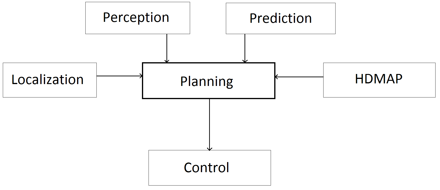
The high-level dataflow of our SD-software is presented on the left of Figure 1. Perception integrates information from multiple sensors (such as cameras, lidars and radars), recognises positions and velocities of other agents as well as static obstacles and traffic light signals and creates a ‘digital representation’ of the traffic situation. This representation is then passed to Prediction which supplies each agent with a bunch of possible trajectories and tries to predict their intentions. All this information is fed to Planning. This block also has access to the current position and velocity of the AV coming from Localization and the information about road surface marking and local traffic rules coming from high-definition maps of the area. Planning guides the AV towards the goal point by repeatedly calculating a trajectory endowed with a velocity profile taking into account the road code and the dynamic environment. The Control module receives an updated trajectory a few times per second and drives the AV along it by interacting with steering and velocity actuators through the CAN bus relying on feedback from Localization.

Figure 1: High-level design of our SD-software and the main parts of its planning unit.

2.2 Main parts of the motion planner

Our motion planner has a three-level architecture with decision making at the end. It consists of the following parts (see Figure 1, on the right). First, a strategic planner provides a bunch of strategic plans for reaching the goal point. A strategic plan is a sequence of actions such as ‘move forward along lane A’ or ‘change from lane B into lane C’. Strategic plans are generated using a combination of path-search techniques in the lane graph of the road network and its sliced version. Then maneuver constructor turns each of these plans into a local planning task (LPT). Examples of LPTs are given in Figure 2.

Figure 2: Examples of LPTs. In (a) the AV has to pass between two parked cars. Maneuver (b) is obtained from a ‘change-left, then change-right’ combination in a strategic plan. This combination serves to drive around obtacles that block the current lane. The $\sqcap$-shaped cut in (b) results from a solid line on the road surface between the lanes that the AV should not cross. In (c) there is a bridge support to the right of the AV, which results in the right road border turning right at right angle. This makes this turn hard to pass.

Each task consists of the initial position of the AV (green rectangle with a bullet inside), a target zone (shown in orange), road borders that the AV should not cross (blue), obstacle areas that must be avoided (red) and penalty zones that increase the path cost. The shape planner solves LPTs and produces an optimal curve on the road surface leading from the initial position of the AV to the target zone avoiding obstacle areas. The velocity planner takes into account dynamic objects and marks the points of the trajectory with timestamps when they should be passed (or equivalently, supplies it with a velocity profile). Sometimes the velocity planner can make a decision to stop at a certain point of the trajectory (e.g. to give way to a pedestrian). Finally, the decision maker or path selector selects one of the calculated trajectories relying on their comfort and safety metrics.

The reason we put the decision module at the end is that in some cases such as lane changing in dynamic environment the right decision can be made only after the trajectories for two possible courses of action (change lane versus push forward) have been fully calculated.

2.3 Interaction with other agents

Based on the shape of a candidate path, others’ intentions and other aspects of the traffic situation we single out four ways of interacting with other agents:

(Ignore) Ignore the agent

(Drive Around) React by changing the shape of trajectory

(Give Way) Stop in front of the agent’s route

(Follow) Move into the agent’s place while keeping distance

For example, we ignore another car if we have right-of-way and the other car moves sufficiently slowly to react and stop. We give way to a pedestrian if they cross the road, but if a pedestrian walks along the edge of a road, we try to overtake it. And if a pedestrian walks away from us in the middle of the road, and we cannot overtake them, then we follow them. Similarly we follow the vehicles which are in front of us and move away from us, but we give way to vehicles that move at angle close to 90 degrees to our trajectory.

Now a few words about how these reactions are implemented. In case of (Ignore) we drive as if the agent did not exist. For (Drive Around) we generate an obstacle area around the agent’s personal space and put it into the corresponding LPT. In (Give Way) and (Follow) we react to an agent by changing not the shape of trajectory but the velocity profile. Thus in these cases no obstacle areas are added to LPTs and so no steering reaction is produced. Instead we reduce the velocity. In (Give Way) we stop the AV in front of other agent’s personal space. In (Follow) we calculate the distance to the agent we must keep for safety and plan our velocity accordingly.

The reason we distinguish between (Give Way) and (Follow) is that in (Give Way) unlike (Follow) one cannot talk about desirable safety distance as a function of velocities of the AV and the other agent.

3 Instances of rule-based decision making

3.1 When to drive around another car?

A naive rule “drive around everything that does not move” may pay off in closed areas with low traffic. In multilane urban roads with dense traffic it leads to unneeded attempts of lane change in situations when the car in front of us becomes stationary, but vehicles in adjacent lanes continue to move. An alternative approach is to put on the map all parking slots and drive around only those stationary cars that overlap with these areas. It may work in locations when parking rules are strictly enforced together with a teleoperation service, which allows a teleoperator to mark particular stationary vehicles as requiring driving around. We also develop a machine learning solution to this decision problem.

3.2 Interacting with cars that overtake ego

By the time we started testing our SD-software on high-speed highways we had tested it for a year in urban environment with traffic often changing from dense to stationary with emphasis on safety. As a consequence, that version of the software produced undesirable braking when other vehicles overtook ego on public highways, because it tried to stabilize the distance faster than human drivers.

It took a few months to change this behavior and thouroughly test a new speed controller for safety. During this period our fleet was supplied with a rule “ignore cars in front of ego if they have non-negative acceleration and move sufficiently faster then ego”, which allowed us to test other components on highway in parallel with the work on the velocity planner.

3.3 Pulling away from oncoming cars

In private roads without median marking it is important to react to oncoming cars by pulling away from them to the roadway edge. It took awhile to figure out the right shape of the corresponding obstacle area. A naive idea to use the same ‘personal space area’ of other vehicles as in other cases of interaction, which is based on the bunch of their possible trajectories, failed for many reasons. First, oncoming cars usually, but not always, pull away from us to their edge of the road, and it is hard to predict this behavior exactly. Second, there is a fundamental difference between interacting with an oncoming car and a static obstacle. If it is not possible to drive around a static obstacle, the AV should produce no steering reaction, but this is not so for and oncoming car, where shifting to the edge of the roadway is always needed. Thirdly, the border of the obstacle area should be parallel to the road edge, as othwerwise the AV does not move close to edge sufficiently long.

These difficulties were overcome by implementing a rule that in presence of an oncoming car generates an obstacle area shaped as a narrow strip along the left border of the driving area. The width of the strip is selected based on the road geometry and the position of the other car in a way to ensure that the resulting LPT has a solution (see Figure 3).

Figure 3: Incorrect (a) and correct (b) obstacle areas for oncoming cars.

3.4 Ignoring pedestrians that do not intend to get in front of AV

It is important to distinguish between pedestrians who intend to cross the road in front of the AV and which require braking reaction and those who do not have such intention (such as C in Figure 4).

Figure 4: Which pedestrians should be ignored ? (B and C, but not A)

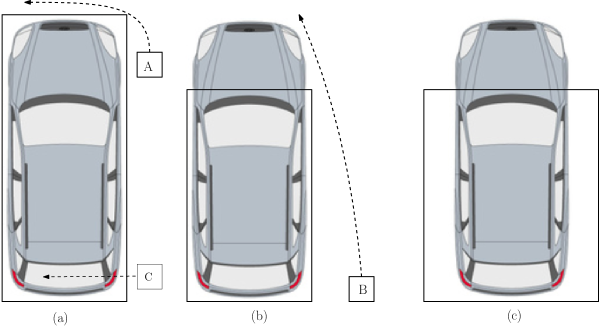
To achieve this we introduced a rule “ignore all pedestrians who collide with the area under the AV”. First this area was taken as in Figure 4, (a), then, after studying a case when pedestrian A was mistakenly ignored, reduced to (b), and then extended on the sides to (c) due to the case with pedestrian B who led to unneeded braking with area (b).

3.5 Rules versus Finite State Machines and Behavior Trees

Consider the rule “extend by additional 25 cm all obstacles that are further than 12 metres from the AV.” This rule may seem counterintutive, but at some point we adopted it as a compromise between giving a hard extension to all objects (which is safer, but may lead to the AV getting stuck in places where a human driver can pass) and driving without extra extension of obstacles. This rule causes the AV to reduce the velocity (up to a stop, if needed) before an obstacle that may require the AV to drive around it, and win time to recognise its position, status, and shape more accurately and calculate the trajectory around it. This two-stage behavior can be coded using such techniques as finite state machines or behaviour trees. However, we prefer the rule-based approach due to its succinctness and the fact that you do not need to specially take care of state change in case there are many cars parked next to each other.

3.6 Yet another controversial rule

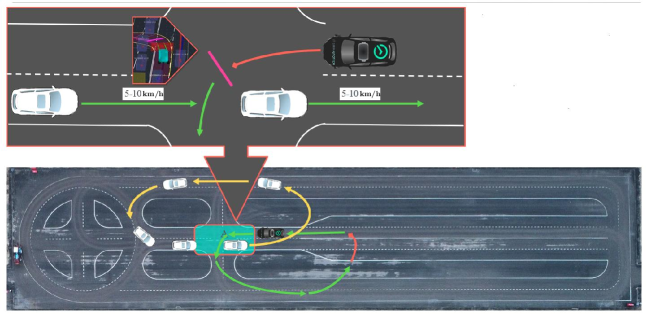
AVs sometimes create dangerous situations by being insufficiently confident during the ‘who goes first’ negotiations. The rule “ignore other vehicle, if we arrive at the collision point by at least 2 seconds earlier” can make their driving style more assertive and closer to that of an average human driver. Given that indiscriminate use of this rule may result in dangerous driving, we believe that at certain situations this or a similar rule can be adopted. Our experiments in the testing ground described in the next section show that it improves performance of the AV by 30 cases out of 260 in a scenario, where it has to turn left through a dense traffic in the opposite lane.

3.7 Give Way or Follow ?

An elegant geometric solution for distinguishing between “give way” and “follow” reactions to other cars was discovered when we faced a junction depicted on the left of Figure 5.

            

Figure 5: Car A is the AV. Car B overtakes us, and so requires (Follow) reaction. On the other hand car C needs a (Give Way) due to local traffic rules.

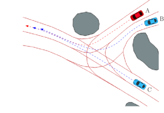
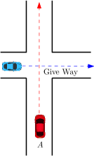
If the other car is on our path, we compare the angle between our and agent’s trajectories with 55 degrees. Otherwise we do the same and, in addition, compare the angle between our and agent’s orientations with 45 degrees. It is readily checked that under this rule we always ‘follow’ car B, but ‘give way’ to car C until it is on our path. This rule also works fine for basic cased on the right of Figure 5.

4 Testing and evaluating the motion planner

Every change in the code of the motion planner undergoes regression testing in a continuous integration platform, which in addition to unit tests runs simulation of the $Prediction+Planning+Control$ part of the SD-pipeline and checks that no collision occur in 10 basic scenarios of interaction with other agents. In addition, the changes in the shape planner are evaluated on a constantly expanding taskset of around 1000 LPTs, where the attention is paid to the distribution of the time required for task solving, special quality features of trajectories (such as distance to obstacles and road border, smoothness, accelerations and jerks), and the rate of tasks that are successfully solved. Finally the change goes into the quality assurance (QA) team, which gives it an hour-long drive in diverse urban environments and logs any noticed defect or change in behavior of the AV. There is also a collection of a few thousands ‘night test’ simulation scenarios which help to track down and correnct rarely occuring regressions.

For A/B testing of different solutions we repeatedly reproduce a traffic situation in the testing ground and count the numbers of cases with acceptable and inacceptable behavior of the AV for each of solutions. An example of such a simulation is shown in Figure 6.

Figure 6: Recreation of the ‘turn left through oncoming traffic’ scenario in the testing ground. The black car is the AV, the white cars simulate dense oncoming traffic. Every fifth white car stops and magnanimously gives way to the AV.

5 Sources of the motion planner

The strategic planner works on network of lanelets introduced in [1]. The maneuver constructor, based on Boost Geometry, seems to be original. The shape planner uses an optimised version of heuristic search from [2] followed by quadratic and Newtonian spline optimization procedures. The velocity planner runs OSQP solver [6] on the s-t-graph of the traffic situation [3] based on predicted trajectories of other vehicles. Path-velocity decomposition dates back to [4]. Our reaction system is inspired by the Mobileye paper on responsibility-sensitive safety [5]. However, most of the rules were created by analysing cases of incorrect interaction with other agents in urban envoronment reported by our QA team.

6 Conclusion

The main purpose of this paper is to attract attention of RR community to practical problems of autonomous driving and demonstrate that designing logical rules that provide robots with spatial intelligence and analysing them integrationally and game-theoretically is an exciting activity. We show that rule-based decision making can play an important role in SD-software by providing use-cases when logical rules helped to improve performance of the motion planner. Also rules provide a nice language for talking about behavior logic of software and analysing bugs: given a case of undesirable behavior, one may say that this or that rule did or did not work as expected, and explain why. Finally, some of the rules can be slots and baselines for plugging machine learning solutions.

References

- [1] Bender, P., Ziegler, J., Stiller, C.: Lanelets: Efficient map representation for autonomous driving. In: 2014 IEEE Intelligent Vehicles Symposium Proc. pp. 420–425
- [2] Botros, A., Smith, S.L.: Multi-start n-dimensional lattice planning with optimal motion primitives. arXiv preprint arXiv:2107.11467 (2021)
- [3] Fan, H., Zhu, F., Liu, C., Zhang, L., Zhuang, L., Li, D., Zhu, W., Hu, J., Li, H., Kong, Q.: Baidu Apollo EM motion planner. arXiv preprint arXiv:1807.08048 (2018)
- [4] Kant, K., Zucker, S.W.: Toward efficient trajectory planning: The path-velocity decomposition. The international journal of robotics research 5(3), 72–89 (1986)
- [5] Shalev-Shwartz, S., Shammah, S., Shashua, A.: On a formal model of safe and scalable self-driving cars. arXiv preprint arXiv:1708.06374 (2017)
- [6] Stellato, B., Banjac, G., Goulart, P., Bemporad, A., Boyd, S.: OSQP: An operator splitting solver for quadratic programs. Mathematical Programming Computation 12(4), 637–672 (2020)