Ranking species in complex ecosystems through nestedness maximization

Abstract

Identifying the rank of species in a social or ecological network is a difficult task, since the rank of each species is invariably determined by complex interactions stipulated with other species. Simply put, the rank of a species is a function of the ranks of all other species through the adjacency matrix of the network. A common system of ranking is to order species in such a way that their neighbours form maximally nested sets, a problem called nested maximization problem (NMP). Here we show that the NMP can be formulated as an instance of the Quadratic Assignment Problem, one of the most important combinatorial optimization problem widely studied in computer science, economics, and operations research. We tackle the problem by Statistical Physics techniques: we derive a set of self-consistent nonlinear equations whose fixed point represents the optimal rankings of species in an arbitrary bipartite mutualistic network, which generalize the Fitness-Complexity equations widely used in the field of economic complexity. Furthermore, we present an efficient algorithm to solve the NMP that outperforms state-of-the-art network-based metrics and genetic algorithms. Eventually, our theoretical framework may be easily generalized to study the relationship between ranking and network structure beyond pairwise interactions, e.g. in higher-order networks.

I Introduction

Experience reveals that species forming complex ecosystems are organized in hierarchies. The ranks of such species, namely their position in the hierarchy, are functions of the interactions encoded in the adjacency matrix of the ecological network. Under this assumption, the task of ranking species can be cast in the problem of finding a suitable permutation of the rows and columns of the adjacency matrix, and this problem is, fundamentally, a combinatorial one. Ranking rows and columns of the adjacency matrix has revealed the existence of nested structures: neighbors of low rank nodes are subsets of the neighbors of high rank nodes Atmar and Patterson [1993], Bascompte et al. [2003], Mariani et al. [2019]. For example, nested patterns are found in the world trade, in which products exported by low-fitness countries constitute subset of those exported by high-fitness countries Tacchella et al. [2012]. In fragmented habitats, species found in the least hospitable islands are a subset of species in the most hospitable islands Atmar and Patterson [1993]. Nestedness in real world interaction networks has captured cross-disciplinary interest for three main reasons. First, nested patterns are ubiquitous among complex systems, ranging from ecological networks Atmar and Patterson [1993], Bascompte et al. [2003] and the human gut microbiome Cobo-López et al. [2022] to socioeconomic systems Tacchella et al. [2012], König et al. [2014] and online social media and collaboration networks Palazzi et al. [2019, 2021]. Second, the ubiquity of nested patterns have triggered intensive debates about the reasons behind the emergence of nestedness in mutualistic systems Suweis et al. [2013], Valverde et al. [2018], Maynard et al. [2018], Cai et al. [2020] and socioeconomic networks König et al. [2014], Palazzi et al. [2021]. Third, nestedness may have profound implications for the stability and dynamics of ecological and economic communities: highly-nested rankings of the nodes have revealed vulnerable species in mutualistic networks Domínguez-García and Munoz [2015] and competitive actors in the world trade Tacchella et al. [2018], Sciarra et al. [2020].

The ubiquity of nestedness and its implications in shaping the structure of biotas have motivated the formulation of the nestedness maximization problem. This problem can be stated in the following way: find the permutation (i.e. ranking) of the rows and columns of the adjacency matrix of the network resulting in a maximally nested layout of the matrix elements. Originally introduced by Atmar and Patterson Atmar and Patterson [1993], the problem has been widely studied in ecology, leading to several algorithms for measuring the nestedness of a matrix, e.g. the popular nestedness temperature calculator and its variants Atmar and Patterson [1993], Rodríguez-Gironés and Santamaría [2006], Almeida-Neto et al. [2007], Payrató-Borràs et al. [2020]. Yet many of these methods do not attempt to optimize the actual cost of a nested solution, but exploit some simple heuristic that is deemed to be correlated with nestedness. Other methods, e.g. BINMATNEST Rodríguez-Gironés and Santamaría [2006], do optimize a nestedness cost following a genetic algorithm, but lack the theoretical insight contained in an analytic solution to the problem. More generally, we lack a formal theory to derive the degree of nestedness of a network from the structure of the adjacency matrix and the ranking of the nodes.

Here, we map the nestedness maximization problem onto the Quadratic Assignement Problem Koopmans and Beckmann [1957], thereby tackling directly the problem of finding the optimal permutation of rows and columns that maximizes the nestedness of the adjacency matrix. In our formulation, the degree of nestedness is measured by a cost function over the space of all possible rows and columns permutations, whose global minimum corresponds to a matrix layout having maximum nestedness. Roughly speaking, the cost function is designed to reward permutations that move the maximum number of non-zero elements of the matrix in the upper left corner and to penalize those that move non-zero elements in the bottom right corner. Next, we set up a theoretical framework which allows us to obtain the mean field solution to the NMP as a leading order approximation and, in principle, calculate also next-to-leading order corrections.

II Problem formulation

We consider bipartite networks where nodes of one kind, representing for example plants indexed by a variable $i=1,...,N$, can only be connected with nodes of another kind, e.g. pollinators indexed by another variable $a=1,...,M$, as seen in Fig. 1a. We denote by $A_{ia}$ the element of the network’s $N\times M$ adjacency matrix: $A_{ia}\neq 0$ if $i$ and $a$ are connected, and $A_{ia}=0$ otherwise. Besides connectivity, the adjacency matrix encodes the interaction strength between nodes such that whenever $i$ and $a$ are connected, the strength of their interaction is $A_{ia}=w_{ia}>0$. A ranking of the rows is represented by a permutation of the integers $\{1,2,...,N\}$, denoted $r\equiv\{r_{1},r_{2},...,r_{N}\}$; a ranking of the columns is represented by a (different) permutation of the integers $\{1,2,...,M\}$, denoted $c\equiv\{c_{1},c_{2},...,c_{M}\}$. More precisely, the $r$ sequence arranges rows in ascending order of their ordinal rankings $r_{i}$ such that row $i$ is ranked higher than row $j$ if $r_{i}<r_{j}$. Similarly, the $c$ sequence arranges columns such that column $a$ ranks higher than column $b$ if $c_{a}<c_{b}$.

To model the problem, one more concept is needed: network nestedness. Nestedness is the property whereby if $j$ ranks lower than $i$, than the neighbors of $j$ form a subset of the neighbors of $i$, as illustrated in Fig. 1b. Different rankings, i.e. different sequences $r$ and $c$, produce different nested patterns, that is, nestedness is a function of the rankings. Therefore, any cost (energy) function that seeks to quantify matrix nestedness must be a function of the rankings $r$ and $c$. The simplest energy function that does the job, aside from trivial cases (see Supplementary Information Sec. VI), is

$$E(r,c)=\sum_{i=1}^{N}\sum_{a=1}^{M}A_{ia}r_{i}c_{a}\ .$$ (1)

The product $A_{ia}r_{i}c_{a}$ penalizes strong interactions between low-rank nodes, since they contribute a large amount to the cost function; thus, low rank nodes typically interact weakly. Strong interactions are only allowed between high rank nodes, because when $A_{ia}$ is large the product $A_{ia}r_{i}c_{a}$ can be made small by choosing $r_{i}$ and $c_{a}$ to be small. Furthermore, high rank nodes can have moderate interactions with low rank nodes, because the product $r_{i}A_{ia}c_{a}$ can be still relatively small when $r_{i}$ is large and $c_{a}$ is small (or viceversa) provided $A_{ia}$ is not too large (hence the name ‘moderate’ interaction).

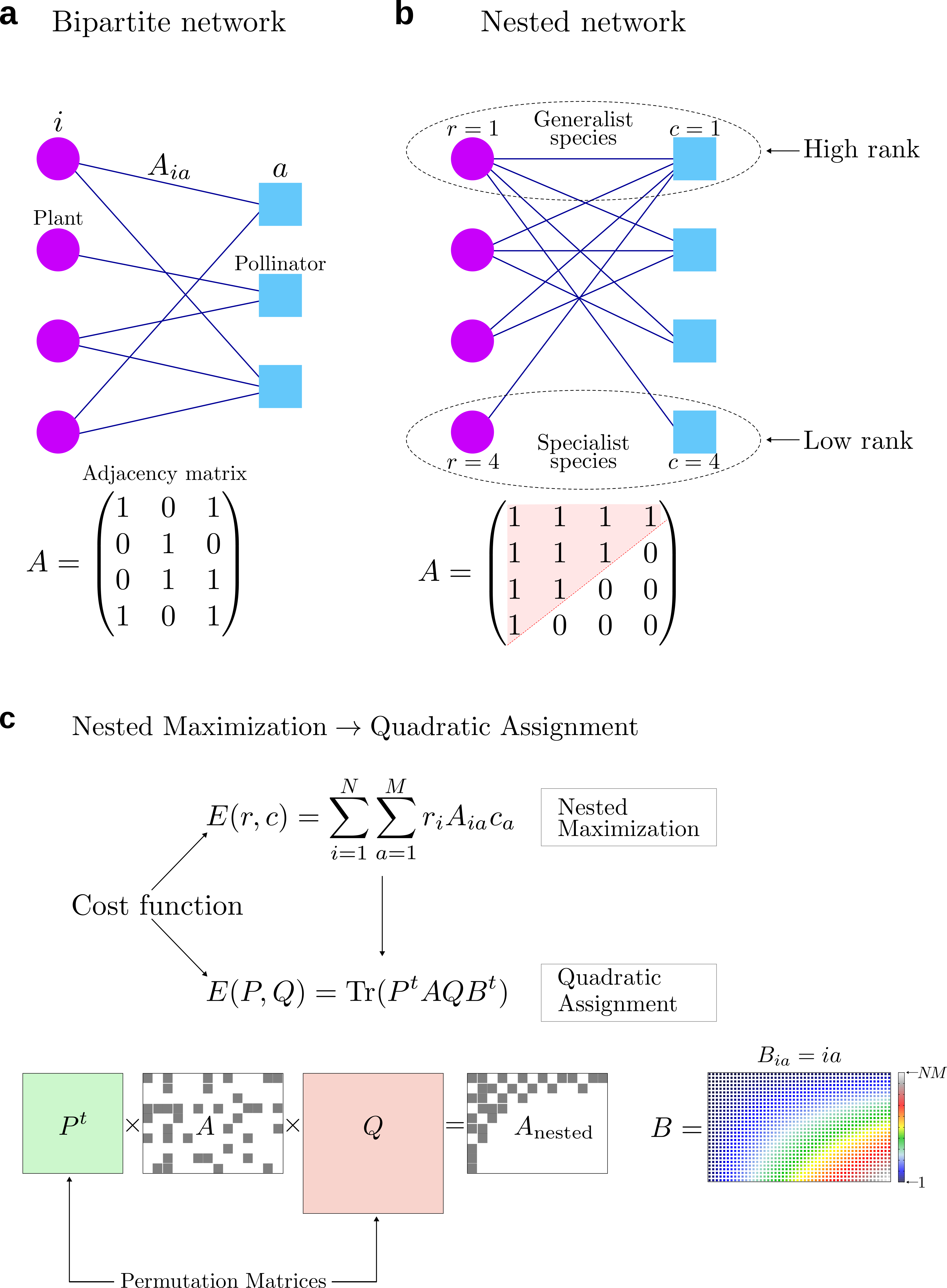
Fig. 1: Modeling of the Nested Maximization Problem. a, A bipartite network models the interactions between, e.g., plants $i$, represented by purple circles, and pollinators $a$, represented by cyan squares, through the adjacency matrix $A$. The interaction is mutualistic, i.e. $A_{ia}=1>0$ if $i$ interacts with $a$ and $A_{ia}=0$ otherwise. b, A nested network has a hierarchical structure wherein the neighbors of low rank nodes (the specialist species at the bottom) are a subset of the neighbors of high rank nodes (the generalists at the top). The rank of a node is encoded in the variables $r_{i}$ (for plants) and $c_{a}$ (for pollinators). Top rank nodes have $r=c-1$, while bottom ones have $r=c=4$. The adjacency matrix of a nested network shows a peculiar pattern with all non-zero entries clustered in the upper left corner. c, Maximizing network nestedness amounts to minimize the cost function $E(r,c)$ over the ranking vectros $r$ and $c$, which, in turn, is equivalent to optimizing the cost $E(P,Q)$ with respect to the permutations matrices $P$ and $Q$. The optimal permutation matrices bring the adjacency matrix to its maximally nested form $P^{t}AQ=A_{\rm nested}$, which is complementary to the layout of matrix $B$.

The assumptions of our model are relevant to diverse scenarios where nestedness has been observed. In bipartite networks of countries connected to their exported products, we could interpret $r_{i}$ as the fitness of country $i$ and $c_{a}$ as the inverse of the complexity of product $a$. In this scenario, high-energy links $r_{i}A_{ia}c_{a}$ represent the higher barriers faced by underdeveloped countries to produce and export sophisticated products Tacchella et al. [2012], whereas low-energy links represent competitive countries exporting ubiquitous products. In mutualistic ecological networks, high-energy links represent the higher extinction risk for specialist pollinators to be connected with specialist plants, whereas low-energy links represent connections within the core of generalist nodes Bascompte et al. [2003] as depicted in Fig. 1b.

With this equipment, it should be clear that to maximize nestedness, we have to minimize the energy function in Eq. (1). More precisely, nestedness maximization is the mathematical optimization problem in which we seek to find the optimal sequences $r^{*}$ and $c^{*}$ that minimize the energy function, i.e. $\min_{r,c}E(r,c)=E(r^{*},c^{*})$. Since the sequence $r$ is a permutation of the ordered sequence $\{1,2,...,N\}$, we can always write $r_{i}=\sum_{n=1}^{N}P_{in}n$, where $P$ is a $N\times N$ permutation matrix. Similarly, we can write $c_{a}=\sum_{m=1}^{M}Q_{am}m$ where $Q$ is a $M\times M$ permutation matrix. Therefore, the energy function, considered as a function of the permutation matrices $P$ and $Q$, can be rewritten in the form

$$E(r,c)=E(P,Q)={\rm Tr}\big{(}P^{t}AQB^{t}\big{)}\ ,$$ (2)

where $B$ is a $N\times M$ matrix with entries $B_{ia}=ia$, as shown in Fig. 1c. In this language, the NMP is simply the problem of finding the permutations $P^{*}$ and $Q^{*}$ that minimize the energy function given by Eq. (2), which mathematically reads

$$(P^{*},Q^{*})=\operatorname*{arg\,min}_{P,\ Q}{E(P,Q)}\ .$$ (3)

The geometric meaning of the optimal permutations $P^{*}$ and $Q^{*}$ is clear if we apply them to the adjacency matrix as $P^{t}AQ=A_{\rm nest}$ in that the nested structure in $A_{\rm nest}$ is visually manifest, as schematized in Fig. 1c. The optimization problem defined by Eqs. (2) and (3) can be recognized as an instance of the Quadratic Assignment Problem (QAP) in the Koopmans-Beckmann form Koopmans and Beckmann [1957], one of the most important problem in combinatorial optimization, that is known to be NP-hard. The formal mathematical mapping of the NMP onto an instance of the QAP represents our first most important result. Having formulated the NMP in the language of permutation matrices, we move next to solve it using a Statistical Physics approach.

III Solving the NMP with Statistical Physics

Our basic tool to study the NMP is the partition function $Z(\beta)$ defined by

$$Z(\beta)=\sum_{P,\ Q}e^{-\beta E(P,Q)}\ ,$$ (4)

where $\beta$ is an external control parameter, akin to the ‘inverse temperature’ in the statistical physics language. The partition function $Z(\beta)$ provides a tool to determine the global minimum of the energy function via the limit

$$E(P^{*},Q^{*})=-\lim_{\beta\to\infty}\frac{1}{\beta}\ln{Z(\beta)}$$ (5)

Calculating the partition function may seem hopeless, since it requires to evaluate and sum up $N!M!$ terms. Nonetheless, the calculation is greatly simplified in the limit of large $\beta$, since we can evaluate $Z(\beta)$ via the steepest descent method. The strategy consists of two main steps. The first step is to work out an integral representation of $Z(\beta)$ of the form

$$Z(\beta)=\int DXDY\ e^{-\beta F(X,Y)}\ ,$$ (6)

where the integral is over the space of $N\times N$ doubly-stochastic (DS) matrices $X$ and $M\times M$ DS matrices $Y$, that converge onto permutation matrices $P$ and $Q$ when $\beta\to\infty$; and $F(X,Y)$ is an “effective cost function” that coincides with $E(P,Q)$ for $\beta\to\infty$. The second step is to find the stationary points of $F(X,Y)$ by zeroing the derivatives $\partial F/\partial X=\partial F/\partial Y=0$, resulting in a set of self-consistent equations for $X$ and $Y$, called saddle point equations. All steps of the calculation are explained in great detail in Supplementary Information VII. The resulting saddle point equations are given by

$$X_{ij} =u_{i}\exp\Big{[}-\beta\big{(}AYB^{t})_{ij}\Big{]}v_{j},$$ (7)

$$Y_{ab} =\mu_{a}\exp\Big{[}-\beta\big{(}A^{t}XB)_{ab}\Big{]}\nu_{b}\ ,$$

where $u,v$ are $N$-dimensional vectors and $\mu,\nu$ are $M$-dimensional vectors determined by imposing that all row and column sums of $X$ and $Y$ are equal to 1. At this point we can exploit the specific form of matrix $B$, i.e. $B_{ia}=ia$, to further simplify Eqs. (7). Specifically, we define the “stochastic” rankings $\rho_{i}$ and $\sigma_{a}$ as

$$\rho_{i}=\sum_{k=1}^{N}X_{ik}\ k\ ,\ \ \ \sigma_{a}=\sum_{b=1}^{M}Y_{ab}\ b\ ,$$ (8)

whereby we can cast Eqs. (7) in the following vectorial form (details in Supplementary Information VII)

$$\rho_{i} =\frac{\sum_{k}k\ v_{k}\ e^{-\beta k\sum_{a}A_{ia}\sigma_{a}}}{\sum_{k}v_{k}\ e^{-\beta k\sum_{a}A_{ia}\sigma_{a}}}\ ,$$ (9)

$$\sigma_{a} =\frac{\sum_{c}c\ \nu_{c}\ e^{-\beta c\sum_{i}A_{ia}\rho_{i}}}{\sum_{c}\nu_{c}\ e^{-\beta c\sum_{i}A_{ia}\rho_{i}}}\ ,$$

where the normalizing vectors $v$ and $\nu$ satisfy

$$\frac{1}{v_{j}}=\sum_{i}\Big{[}\sum_{k}\ v_{k}\ e^{-\beta(k-j)\sum_{a}A_{ia}\sigma_{a}}\Big{]}^{-1}\ ,$$ (10)

$$\frac{1}{\nu_{b}}=\sum_{a}\Big{[}\sum_{c}\ \nu_{c}\ e^{-\beta(c-b)\sum_{i}A_{ia}\rho_{i}}\Big{]}^{-1}\ .$$

Equations (9) and (10) represent our second most important result and, when interpreted as iterative equations, provide a simple algorithm to solve the NMP, whose implementation is discussed in detail in Supplementary Information VIII. Note that $\rho$ and $\sigma$ converge to the the actual ranking $r$ and $s$ for $\beta\to\infty$. However, in practice, we solve Eqs. (9) and (10) iteratively at finite $\beta$. Once we reach convergence, we estimate $r$ and $s$ by simply sorting the entries of $\rho$ and $\sigma$. We observe that larger values of $\beta$ give better results, i.e., lower values of the cost $E(r,s)$, as seen in Fig. 2a. A full discussion of convergence and bounds of our algorithm will be published elsewhere. Here, we test its performance by applying it to many real mutualistic networks and show that we obtain better results than state-of-the-art network metrics and genetic algorithms, as discussed next.

IV Numerical results

We apply our algorithm on 47 real mutualistic networks freely downloadable at https://www.web-of-life.es/, whose filenames can be found in the first column of Table 1. To standardize the comparison with existing methods, we binarize the adjacency matrices of the networks setting $A_{ij}=1$ if nodes $i$ and $j$ are connected and zero otherwise, thus ignoring the weights. Despite this simplification, we like to emphasize that our algorithm can be applied, as is, to any mutualistic weighted network of the most general form. Then we run four different algorithms comprising: naive degree Araujo et al. [2010], fitness-complexity (FC) Tacchella et al. [2012], minimal extremal metric (MEM) Wu et al. [2016], and BINMATNEST Rodríguez-Gironés and Santamaría [2006]. While BINMATNEST is the state-of-the-art algorithm in ecology for nestedness maximization Dormann [2020], the effectiveness of the FC Lin et al. [2018], Mazzilli et al. [2022] and MEM Wu et al. [2016] has been proved in recent works in economic complexity, which also connected the FC to the Sinkhorn algorithm from optimal transport Sinkhorn and Knopp [1967], Marshall and Olkin [1968], Mazzilli et al. [2022]. We compare the value of the cost function $E(r,c)$ returned by each of the analyzed algorithms to the value returned by our algorithm (see Supplementary Information Sec. VI for implementation details). As shown in Fig. 2b, our algorithm finds a better (i.e. lower) cost than degree, FC, and MEM on $100\%$ of the networks. When compared to BINMATNEST, we find a better (or equal) minimum cost in $80\%$ of the instances, as seen in Fig. 2b and Table 1.

We conclude this section by showing an application of the similarity transformation that brings the adjacency matrix to its maximally nested form. We call $P$ and $Q$ the optimal permutations that solve the QAP in Eq. (3) (details in Supplementary Information Sec. VIII) and we perform the similarity trasformation

$$A\to P^{t}AQ\ ,$$ (11)

which reveals the nested structure of the adjacency matrix shown in Fig. 2c.

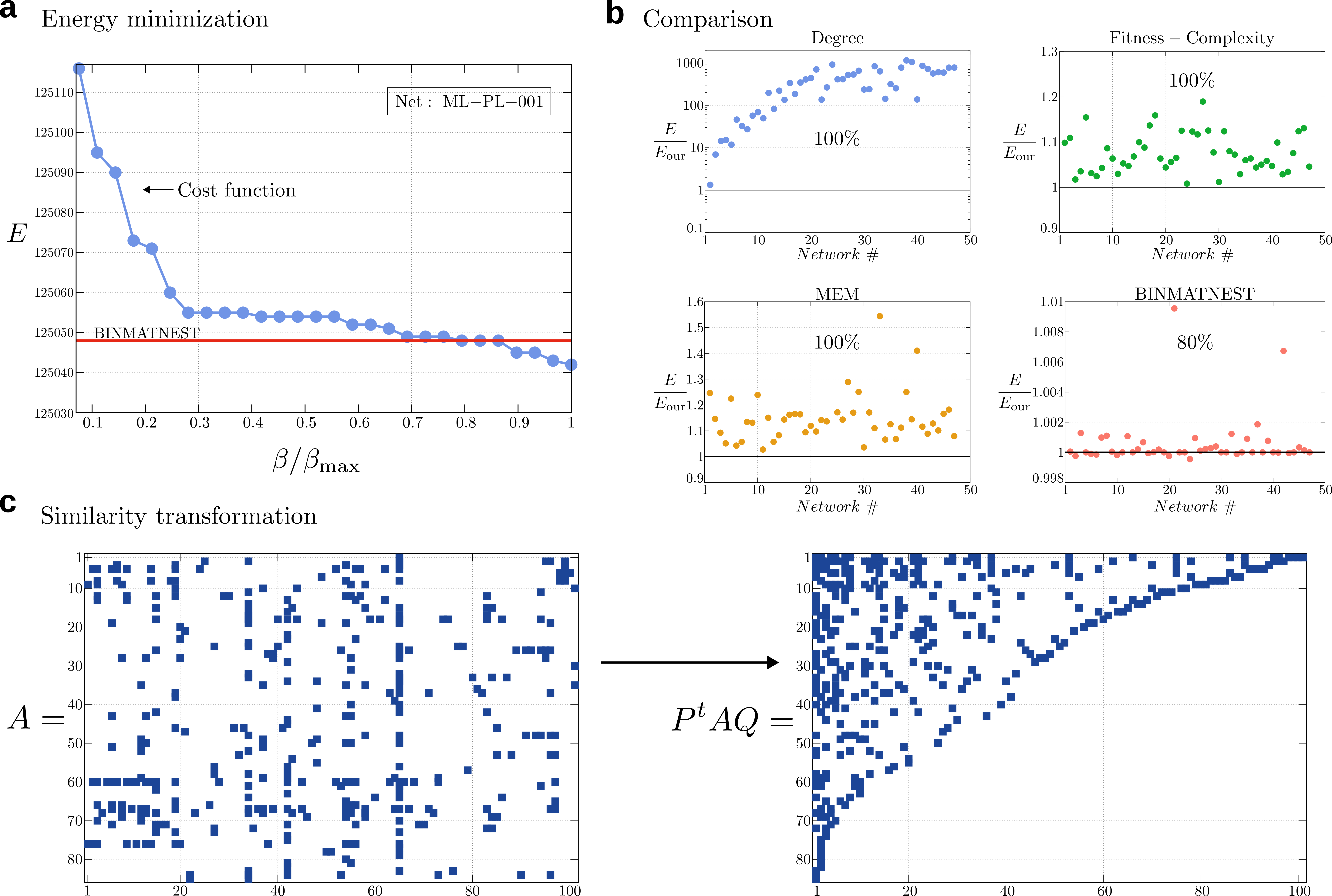
Fig. 2: Numerical solution and comparison with other methods. a, Optimal cost $E(r,c)$ returned by our algorithm on the mutualistic network named ML-PL-OO1 in the Web-of-Life database, for several choices of the parameter $\beta$. Larger values of $\beta$ give lower costs. In particular, for sufficiently large $\beta$ our algorithm returns a lower cost than the best off-the-shelf algorithm for nestedness maximization (BINMATNEST, red line). b, Comparison of our algorithm with state-of-the-art methods in the literature: Degree (upper-left), Fitness-Complexity (upper-right), Minimal-Extremal-Metric (bottom-left) , and BINMATNEST (bottom-right). In each panel we plot the cost returned by each algorithm divided by the cost returned by our algorithm, denoted $E/E_{\rm our}$, for each network considered in this work. A value $E/E_{\rm our}>1$ means that our algorithm returns a better, i.e. lower, cost. We find that our algorithm returns a better cost in $100\%$ of the networks when compared to degree, FC, and MEM, and in $80\%$ of the networks when compared to BINMATNEST (see also Table 1). c, Similarity transformation applied to the adjacency matrix $A$ of network ML-PL-OO1 that brings $A$ into its maximally nested form $P^{t}AQ$, where $P$ and $Q$ are the optimal permutation matrices constructed from the optimal ranking vectors $r^{*}$ and $s^{*}$.

V Conclusions

In this work we introduced a cost function for the NMP in bipartite mutualistic networks. This formulation allowed us to recast the problem as an instance of the QAP, that we tackled by Statistical Physics techniques. In particular, we obtained a mean field solution by using the steepest-descent approximation of the partition function. The corresponding saddle-point equations depend on a single hyper-parameter (the inverse temperature $\beta$) and can be solved by iteration to find the optimal rankings of the rows and columns of the adjacency matrix that result in a maximally nested layout. We benchmarked our algorithm against other methods on several real ecological networks and showed that our algorithm outperforms the best existing algorithm in $80\%$ of the instances.

We note that by changing the definition of the matrix $B$, i.e. using measures other than a sequence of ordinal numbers, one can repurpose our algorithm to rank rows and columns of a matrix according to other geometric patterns Morone [2022], De Bacco et al. [2018]. Therefore, the proposed framework holds promise for the effective detection of a wide range of network structural patterns beyond the nestedness considered here. Finally, the present framework can be easily extended and applied to solve the ranking problem in networks with higher order interactions. For example, given the adjacency tensor $A_{ia\gamma}$ for a system with $3$-body interactions, we can define the energy function $E(P,Q,R)$ to be optimized over $3$ permutation matrices $P$, $Q$, and $R$ following exactly the same steps outlined in this paper for the case of pairwise interactions. This may be especially relevant in the world trade for ranking countries according to both exported and imported goods.

Net	N	M	$||A||/NM$	FC	DEG	MEM	BIT	OUR
M-PL-001	84	101	0.042551	137348	165930	155841	125048	125042
M-PL-002	43	64	0.071221	37556	232827	38823	33850	33858
M-PL-003	36	25	0.090000	3927	55335	4220	3866	3862
M-PL-004	12	102	0.136438	12082	176999	12274	11672	11672
M-PL-005	96	275	0.034962	885890	9040760	939937	767320	767393
M-PL-006	17	61	0.140791	6579	293503	6653	6379	6379
M-PL-007	16	36	0.147569	3109	98372	3210	3038	3036
M-PL-008	11	38	0.253589	5654	148325	6153	5428	5422
M-PL-009	24	118	0.085452	48398	2535535	50418	44559	44556
M-PL-010	31	76	0.193548	103649	6714987	120773	97454	97472
M-PL-011	14	13	0.285714	970	46815	968	943	943
M-PL-012	29	55	0.090909	9948	1861449	10871	9460	9449
M-PL-013	9	56	0.204365	4863	383760	4910	4644	4644
M-PL-014	29	81	0.076203	20106	4179783	20387	18830	18827
M-PL-016	26	179	0.088526	122835	15019420	127784	111800	111725
M-PL-017	25	79	0.151392	35393	10925775	37814	32533	32534
M-PL-018	39	105	0.093529	121642	19872497	124677	107023	107022
M-PL-019	40	85	0.077647	56643	16872116	56890	48888	48879
M-PL-020	20	91	0.104396	17037	6545141	17540	16022	16022
M-PL-022	21	45	0.087831	4339	1833172	4655	4156	4158
M-PL-023	23	72	0.075483	9513	6341662	9890	9098	9011
M-PL-024	11	18	0.191919	803	103022	862	755	755
M-PL-025	13	44	0.250000	8148	1921580	8233	7243	7243
M-PL-026	105	54	0.035979	17998	16395570	56197	17847	17855
M-PL-027	18	60	0.111111	14188	5208823	14803	12644	12633
M-PL-028	41	139	0.065626	126748	46897882	129783	113503	113490
M-PL-029	49	118	0.059841	105634	46529364	114448	88825	88805
M-PL-030	28	53	0.073450	15658	7451270	16284	13918	13915

Net	N	M	$||A||/NM$	FC	DEG	MEM	BIT	OUR
M-PL-031	48	49	0.066327	24134	14712154	28025	22418	22409
M-PL-032	7	33	0.281385	1379	322338	1413	1363	1363
M-PL-033	13	34	0.319005	9718	2086383	10128	8648	8648
M-PL-034	26	128	0.093750	48523	37671897	49907	44993	44938
M-PL-035	61	36	0.081056	19907	11775325	28663	18565	18567
M-PL-036	10	12	0.250000	465	64621	483	452	452
M-PL-037	10	40	0.180000	3543	1061073	3763	3346	3342
M-PL-038	8	42	0.235119	3616	860044	3631	3399	3399
M-PL-039	17	51	0.148789	8400	6259559	8956	8065	8050
M-PL-040	29	43	0.091419	8126	8906049	9676	7739	7739
M-PL-041	31	43	0.108777	12445	12353208	13463	11771	11761
M-PL-042	12	6	0.347222	221	29225	298	212	212
M-PL-043	28	82	0.108885	46324	36103187	47058	42156	42156
M-PL-045	17	26	0.142534	1833	1291777	1941	1795	1783
M-PL-046	16	44	0.394886	23365	12810171	25494	22591	22592
M-PL-047	19	186	0.120260	82943	46841210	84968	77126	77126
M-PL-048	30	236	0.094774	273971	144577341	284223	243852	243771
M-PL-049	37	225	0.070871	255534	175524328	267224	226068	226039
M-PL-050	14	35	0.175510	3467	2586805	3581	3317	3317

Table 1: Numerical results on real mutualistic networks from the Web of Life database. First tab is the filename of the network as it appears in the database. Second and third tabs are the number of rows and columns, respectively. Fourth tab is the norm of the (binarized) adjacency matrix (sum of non zero entries) divided by $NM$. Last five tabs represent the minimum cost returned by, in order, Fitness-Complexity, Degree, Minimal Extremal Metric, BINMATNEST and our method. We highlight in blue the best result among these five methods.

Data availability Data that support the findings of this study are publicly available at the Web of Life database at https://www.web-of-life.es/

Acknowledgments This work was partially supported by AFOSR: Grant FA9550-21-1-0236. MSM acknowledges financial support from the URPP Social Networks at the University of Zurich, and the Swiss National Science Foundation, Grant 100013-207888.

Author contributions All authors contributed equally to this work.

Additional information Supplementary Information accompanies this paper.

Competing interests

The authors declare no competing interests.

Correspondence should be addressed to F. M. at: fm2452@nyu.edu

Supplementary Information for:

Ranking species in complex ecosystems through nestedness maximization

Manuel Sebastian Mariani, Dario Mazzilli, Aurelio Patelli & Flaviano Morone

VI Related Works

In this section we briefly review existing methods, models, and algorithms tackling the ranking and nestedness maximization problems.

VI.1 Ranking by degree

The degree of a node is simply defined as its number of connections. It can be connected to a nestedness maximization problem as follows. In Ref. Araujo et al. [2010] the authors consider the following energy function

$$E(\vec{r},\vec{s})=\sum_{i,a}A_{ia}(r_{i}+s_{a})\ .$$ (12)

The meaning of this energy function can be easily understood when $A_{ia}\in\{0,1\}$. In this case the sum can be rewritten as: $\sum_{ia}A_{ia}(r_{i}+s_{a})=\sum_{i}k_{i}r_{i}+\sum_{a}k_{a}s_{a}$, where $k_{i}$ and $k_{a}$ are the degrees (number of connections) of nodes $i$ and $a$, respectively. In the language of statistical physics the term $k_{i}r_{i}$ represents an interaction between the degrees of freedom $r_{i}$ and a local magnetic field $k_{i}$, whose intensity equals the node’s degree. The stronger the magnetic field $k_{i}$ is, the lower the value of $r_{i}$ ought to be in order to minimize the product $r_{i}k_{i}$. This reasoning can be generalized to the case $A_{ia}\in\{0,w_{ia}\}$ upon changing the definition of the magnetic field from the node degree to the weighted node degree, the weights being the interaction strengths $w_{ia}$. In both cases, the effect of this term is to assign high rank to nodes with high values of $k_{i}$ (or $k_{a}$ of course).

The non-interacting energy function defined in (12) is minimized by ranking the nodes according to their degree, and can be seen as an instance of the Linear Assignment Problem, whose solution can be found in polynomial time (in this case by simply sorting the degrees, so in $O(N\log N)$ operations). Authors of Ref. Araujo et al. [2010] only considered the rankings of nodes by degree, and they were interested in comparing the energy observed in empirical networks against that of idealized nested structures. In our framework, we model the nestedness maximization problem by an energy function that couples the rows and columns’ ranking positions, which can be seen as an instance of the Quadratic Assignment Problem Koopmans and Beckmann [1957], which is known to be NP-hard, and thus there is no known algorithm that can find the optimal solution in polynomial time.

VI.2 SpringRank

Reference De Bacco et al. [2018] considered an energy-based approach to rank nodes in directed weighted unipartite networks. They defined $A_{ij}$ as the number of interactions suggesting that $i$ is ranked above $j$, and they defined the SpringRank centrality as the vector $\vec{\eta}^{*}$ of real-valued scores that minimize the energy function

$$E(\vec{\eta})=\sum_{i,j}A_{ij}(\eta_{i}-\eta_{j}+1)^{2}\ .$$ (13)

The model reflects the assumption that if many directed interactions suggesting that $i$ is ranked above $j$ are observed, then the centrality of $i$ should be much larger than that of $j$. Subsequently, the authors develop statistical inference techniques to infer the node-level SpringRank scores in empirical networks. Broadly speaking, their approach is conceptually related to ours as it defines the rankings of the nodes in terms of the minimum of an energy function that depends on the nodes scores and the network’s adjacency matrix. However, their ranking method focuses on directed weighted unipartite networks and it does not aim at maximizing the network nestedness, and therefore it won’t be compared to the method presented in this work.

VI.3 BINMATNEST

BINMATNEST Rodríguez-Gironés and Santamaría [2006] can be considered as the state-of-the-art algorithm to maximize nestedness in ecology Dormann [2020]. In fact, the algorithm minimizes the nestedness temperature Atmar and Patterson [1993], a variable that is conceptually related to the nestedness energy defined in the main text. The nestedness temperature $T$ quantifies the average distance of the adjacency matrix’s elements from the so-called isocline of perfect nestedness, which represents the separatrix between the empty and filled regions of a perfectly-nested matrix with the same density as the original matrix. We refer to Rodríguez-Gironés and Santamaría [2006] for details of the isocline determination and temperature calculation. Of course $T$ depends on the adjacency matrix $A$ as well as the permutation of its rows and columns. The dependence of $T$ on the ranking vectors is more complex than the nestedness energy function introduced here, and therefore, its optimization less amenable to analytic treatment. The genetic algorithm BINMATNEST bypasses the problem by relying on an iterative algorithm.

In BINMATNEST Rodríguez-Gironés and Santamaría [2006], a candidate solution is represented by the rankings’ vectors $r=\{r_{1},r_{2},…,r_{N}\}$ and $c=\{c_{1},c_{2},…,c_{M}\}$. One starts from a population of initial solutions, composed of the original matrix, solutions found with a similar algorithm as the original one by Atmar and Patterson Atmar and Patterson [1993], and their mutations. From a well-performing candidate solution, an offspring of solution is created by selecting a second “parent” from the remaining solutions in the population, suitably combining the information from the two solutions, and eventually performing random mutations in the resulting child solution. Specifically, denote as $w$ the row ranking vector of a well-performing solution and $p$ the row ranking vector of its selected partner (the procedure is analogous for the column ranking vectors). The row ranking vector of the offspring solution, $o$, is set to $w$ with probability $0.5$, otherwise it is determined by a combination of $w$ and $p$ determined by the following algorithm Rodríguez-Gironés and Santamaría [2006]:

• An integer $k\in\{1,\dots,N\}$ is selected uniformly at random.

• We set $o_{i}=w_{i}$ for all $i\in\{1,\dots,k\}$.

• For $i\in\{k+1,\dots,N\}$, if $p_{i}\notin\{w_{i},\dots,w_{k}\}$, then we set $o_{i}=p_{i}$.

• For $i\in\{k+1,\dots,N\}$, if $p_{i}\in\{w_{i},\dots,w_{k}\}$, then the value of $o_{i}$ is chosen at random from all the unused positions.

As final step, a random mutation of ranking vector $o$ is performed by selecting at random $k_{1},k_{2}\in\{1,\dots,N\}$ and performing a cyclical permutation of the elements $r_{k_{1}},\dots,r_{k_{2}}$. For both rows and columns, the procedure is repeated for a prefixed number of iterations, and the lowest-temperature candidate solution $(r^{*},c^{*})$ is then chosen as the final solution. In our study, we run the BINMATNEST algorithm through the nestedrank function of the bipartite R package .

VI.4 Fitness-complexity

The fitness-complexity algorithm has been introduced to simultanoeusly measure the economic competitivenss of countries ($f_{i}\in[0,\infty)$) and the sophistication of products ($q_{\alpha}\in[0,\infty$) from the bipartite network connecting the countries with the products they export in world trade Tacchella et al. [2012]. The original fitness-complexity equations read Tacchella et al. [2012]

$$\begin{split}f_{i}^{-1}&=x_{i}=\frac{1}{\sum_{a}A_{ia}\,q_{a}}\\ q_{a}&=y_{a}=\frac{1}{\sum_{i}A_{ia}\,x_{i}},\end{split}$$ (14)

which implies that high-fitness countries export many products – both high- and low-complexity ones – and high-complexity products are rarely exported by low-fitness countries. We observe that the fitness-complexity equations are formally equivalent to the Sinkhorn-Knopp equations used in optimal transport Sinkhorn and Knopp [1967], Mazzilli et al. [2022]. As such, they can be derived by solving a quadratic optimization problem with logarithmic barriers, defined by the energy function Marshall and Olkin [1968]

$$E=\sum_{i,a}A_{ia}\,x_{i}\,y_{a}-\sum_{i}\log x_{i}-\sum_{\alpha}\log y_{a}.$$ (15)

By taking the partial derivatives of $E(\mathbf{x},\mathbf{y})$ with respect to $x_{i}$ and $y_{\alpha}$, respectively, we obtain indeed the fitness-complexity equations in Eq. (14). This remark provides an optimization-based interpretation of the fitness-complexity equations, while it does not provide a principled interpretation for the logarithmic barriers and the relation between the fitness-complexity scores and the degree of nestedness of a network. The algorithm has been shown to effectively pack bipartite adjacency matrices into nested configurations through both qualitative and quantitative arguments Tacchella et al. [2012], Lin et al. [2018], which motivates its inclusion in our paper.

VI.5 Minimal extremal metric

The minimal extremal metric (MEM) is a variant of the fitness-complexity algorithm that penalizes more heavily products exported by low-fitness countries. The MEM equations read Wu et al. [2016]

$$\begin{split}f_{i}^{-1}&=x_{i}=\frac{1}{\sum_{a}A_{ia}\,q_{a}}\\ q_{a}&=y_{a}=\min_{i:A_{ia}=1}\{F_{i}\},\end{split}$$ (16)

which implies high-complexity products are never exported by low-fitness countries. The metric has been shown to visually pack bipartite adjacency matrices better than the original FC algorithm Wu et al. [2016], which motivates its inclusion in our paper.

VII Derivation of the saddle point equations

In this section we discuss in detail how to derive the saddle point Eqs. (7) given in the main text. We consider the minimization problem defined by

$$(r^{*},s^{*})=\operatorname*{arg\,min}_{r\in\mathcal{R}_{N},s\in\mathcal{R}_{M})}{E(r,s)}\ ,$$ (17)

where the cost (energy) function is given by

$$E=\sum_{i=1}^{N}\sum_{a=1}^{M}A_{ia}\,r_{i}\,s_{a}\ ,$$ (18)

and $\mathcal{R}_{N}$ and $\mathcal{R}_{M}$ are the sets of all vectors $r$ and $s$ obtained by permuting the entries of the representative vectors $r^{0}$ and $s^{0}$ defined as

$$r^{0} \equiv(1,2,3,...,N)\ ,$$ (19)

$$s^{0} \equiv(1,2,3,...,M)\ .$$

Therefore, we can write any two vectors $r$ and $s$ as

$$r_{i} =\sum_{j=1}^{N}P_{ij}r^{0}_{j},$$ (20)

$$s_{a} =\sum_{a=1}^{M}Q_{ab}s^{0}_{b}\ ,$$

where $P$ and $Q$ are arbitrary permutation matrices of size $N\times N$ and $M\times M$, respectively. Furthermore, we introduce the $N\times M$ matrix $B$ defined as the tensor product of $r^{0}$ and $s^{0}$, whose components are explicitly given by

$$B_{ia}=(r^{0}\otimes s^{0})_{ia}=ia\ .$$ (21)

With these definitions we can rewrite the energy function as the trace of a product of matrices in the following way:

$$E\equiv E(P,Q)={\rm Tr}(P^{t}AQB^{t})\ .$$ (22)

The minimization problem in Eq. (17) can be reformulated as a minimization problem in the space of permutation matrices as follows

$$(P^{*},Q^{*})=\operatorname*{arg\,min}_{(P\in\mathcal{S}_{N},\ Q\in\mathcal{S}_{M})}{E(P,Q)}\ ,$$ (23)

where $\mathcal{S}_{N}$ and $\mathcal{S}_{M}$ denote the symmetric groups on $N$ and $M$ elements, respectively.

Next we discuss a relaxation of the problem in Eq. (23) that amounts to extend the spaces $\mathcal{S}_{N}$ and $\mathcal{S}_{M}$ of permutation matrices onto the spaces of doubly-stochastic (DS) matrices $\mathcal{D}_{N}$ and $\mathcal{D}_{M}$. The space $\mathcal{D}_{N}$ ($\mathcal{D}_{M}$) is a superset of the original space $\mathcal{S}_{N}$ ($\mathcal{S}_{M}$). Solving the problem on the $\mathcal{D}$-space means to find two doubly-stochastic matrices $X^{*}$ and $Y^{*}$ that minimize an ‘effective’ cost function $F$, i.e.

$$F(X^{*},Y^{*})=\min_{(X\in\mathcal{D}_{N},\ Y\in\mathcal{D}_{M})}{F(X,Y)}\ ,$$ (24)

and are only ‘slightly different’ from the permutation matrices $P^{*}$ and $Q^{*}$ (we will specify later what ‘slightly different’ means in mathematical terms and what $F$ actually is). The quantity which plays the fundamental role in the relaxation procedure of the original problem is the partition function, $Z(\beta)$, defined by

$$Z(\beta)=\sum_{P\in\mathcal{S}_{N}}\sum_{Q\in\mathcal{S}_{M}}e^{-\beta E(P,Q)}\ .$$ (25)

The connection between $Z(\beta)$ and the original problem in Eq. (23) is established by the following limit:

$$\lim_{\beta\to\infty}-\frac{1}{\beta}\log Z(\beta)=\min_{(P\in\mathcal{S}_{N},\ Q\in\mathcal{S}_{M})}{E(P,Q)}\ .$$ (26)

The optimization problem in Eq. (23) is thus equivalent to the problem of calculating the partition function in Eq. (25). Ideally, we would like to compute exactly $Z(\beta)$ for arbitrary $\beta$ and then take the limit $\beta\to\infty$. Although an exact calculation of the partition function is, in general, out of reach, in practice we may well expect that the better we estimate $Z(\beta)$, the closer the limit in Eq. (26) will be to the true optimal solution. In fact, the procedure of relaxation is basically a procedure to assess the partition function for large but finite $\beta$. Mathematically, this procedure is called method of steepest descent debye . By estimating the partition function via the steepest descent method we will obtain a system of non-linear equations, called saddle-point equations, whose solution is a pair of doubly-stochastic matrices $X^{*},Y^{*}$ that solve the relaxed problem given by Eq. (24). Eventually, the solution to the original problem in Eq. (23) can be obtained formally by projecting $X^{*},Y^{*}$ onto the subspaces $\mathcal{S}_{N},\mathcal{S}_{M}\subset\mathcal{D}_{N},\mathcal{D}_{M}$ via the limit

$$\lim_{\beta\to\infty}X^{*}(\beta) =P^{*}\ ,$$ (27)

$$\lim_{\beta\to\infty}Y^{*}(\beta) =Q^{*}\ .$$

Having explained the rationale for the introduction of the partition function, we move next to discuss the details of the calculation leading to the saddle point equations.

In order to cast the partition function in a form suitable for the steepest-descent evaluation, we need the following preliminary result.

Definition: Semi-permutation matrix: a $N\times N$ square matrix $\not{P}$ is called a semi-permutation matrix if $\not{P}_{ij}\in\{0,1\}$ and each row sums to one, i.e. $\sum_{j=1}^{N}\not{P}_{ij}=1$ for $i=1,...,N$, but no further constraint on the column sums is imposed.

We denote $\mathcal{\not{S}}_{N}$ the space of semi-permutation matrices:

$$\mathcal{\not{S}}_{N}=\Bigg{\{}\not{P}\ |\ \not{P}_{ij}\in\{0,1\}\ {\rm AND\ }\sum_{j=1}^{N}\not{P}_{ij}=1\ \forall i\Bigg{\}}$$ (28)

Lemma

Consider an arbitary $N\times N$ square matrix $G$ and the function $W(G)$ defined by

$$e^{W(G)}=\sum_{\not{P}\in\mathcal{\not{S}}_{N}}e^{{\rm Tr}(\not{P}G^{t})}\ .$$ (29)

Then, $W(G)$ is explicitly given by the following formula

$$\boxed{\ W(G)=\sum_{i=1}^{N}\log\sum_{j=1}^{N}e^{G_{ij}}\ }\ .$$ (30)

Proof

Let us write the right hand side of Eq. (29) as

$$\sum_{\not{P}\in\mathcal{\not{S}}_{N}}e^{\sum_{ij}\not{P}_{ij}G_{ij}}=\sum_{\not{P}_{1}}e^{\sum_{j}(\not{P}_{1})_{j}G_{1j}}\sum_{\not{P}_{2}}e^{\sum_{j}(\not{P}_{2})_{j}G_{2j}}\ \ldots\ ,$$ (31)

where $\not{P}_{i}$ is the ${\rm i}^{\rm th}$ row of $\not{P}$ (and thus is a vector) having one component equal to $1$ and the remaining $N-1$ components equal to $0$. The sum $\sum_{\not{P}_{i}}$ denotes a summation over all possible choices of the vector $\not{P}_{i}$: there are $N$ possible such choices, namely $\not{P}_{i}=(1,0,...,0)$, $\not{P}_{i}=(0,1,...,0),...,\not{P}_{i}=(0,0,...,1)$. Hence, each sum in the right hand side of Eq. (31) evaluates

$$\sum_{\not{P}_{i}}e^{\sum_{j}(\not{P}_{i})_{j}G_{ij}}=e^{G_{i1}}+e^{G_{i2}}+...=\sum_{j=1}^{N}e^{G_{ij}}\ .$$ (32)

Thus, the left hand side of Eq. (31) is equal to

$$\sum_{\not{P}\in\mathcal{\not{S}}_{N}}e^{\sum_{ij}\not{P}_{ij}G_{ij}}=\prod_{i=1}^{N}\sum_{j=1}^{N}e^{G_{ij}}\ .$$ (33)

Eventually, by taking the logarithm of both sides of Eq. (33), we prove Eq. (30).

With these tools at hand we move to derive the integral representation of $Z(\beta)$.

Integral representation of $Z(\beta)$

We use the definition of the Dirac $\delta$-function to write the partition function in Eq. (25) as follows

$$Z(\beta)=\sum_{P\in\mathcal{S}_{N}}\sum_{Q\in\mathcal{S}_{M}}\int DX\int DYe^{-\beta E(X,Y)}\prod_{i,j=1}^{N}\delta(X_{ij}-P_{ij})\prod_{a,b=1}^{N}\delta(Y_{ab}-Q_{ab})\ ,$$ (34)

where the integration measures are defined by $DX\equiv\prod_{i,j}dX_{ij}$ and $DY\equiv\prod_{a,b}dY_{ab}$. The next step is to transform the sum over permutation matrices $P,Q$ into a sum over semi-permutations matrices $\not{P},\not{Q}$ and then performing explicitly this sum using the Lemma in Eq. (30). In order to achieve this goal, we insert into Eq. (34) $N$ delta functions $\prod_{j=1}^{N}\delta\Big{(}\sum_{i}X_{ij}-1\Big{)}$ and $M$ delta functions $\prod_{b=1}^{M}\delta\Big{(}\sum_{a}Y_{ab}-1\Big{)}$ to enforce the conditions that the columns of $X$ and $Y$ do sum up to one. By inserting these delta functions, we can then replace the sum over $P,Q$ by a sum over $\not{P},\not{Q}$, thus obtaining

$$Z(\beta)=\sum_{\not{P}}\sum_{\not{Q}}\int DXDYe^{-\beta E(X,Y)}\prod_{i,j=1}^{N}\delta(X_{ij}-\not{P}_{ij})\prod_{a,b=1}^{N}\delta(Y_{ab}-\not{Q}_{ab})\prod_{j=1}^{N}\delta\Big{(}\sum_{i}X_{ij}-1\Big{)}\prod_{b=1}^{M}\delta\Big{(}\sum_{a}Y_{ab}-1\Big{)}\ .$$ (35)

To proceed further in the calculation, we use the following integral representations of the delta-functions:

$$\delta(X_{ij}-\not{P}_{ij}) =\frac{1}{2\pi i}\int_{-i\infty}^{i\infty}d\hat{X}_{ij}\ e^{-\hat{X}_{ij}(X_{ij}-\not{P}_{ij})}\ ,$$ (36)

$$\delta(Y_{ab}-\not{Q}_{ab}) =\frac{1}{2\pi i}\int_{-i\infty}^{i\infty}d\hat{Y}_{ab}\ e^{-\hat{Y}_{ab}(Y_{ab}-\not{Q}_{ab})}\ ,$$

$$\delta\Big{(}\sum_{i}X_{ij}-1\Big{)} =\frac{1}{2\pi i}\int_{-i\infty}^{i\infty}dz_{j}\ e^{-z_{j}\big{(}\sum_{i}X_{ij}-1\big{)}}\ ,$$

$$\delta\Big{(}\sum_{a}Y_{ab}-1\Big{)} =\frac{1}{2\pi i}\int_{-i\infty}^{i\infty}dw_{b}\ e^{-w_{b}\big{(}\sum_{a}Y_{ab}-1\big{)}}\ ,$$

into Eq. (35) and we get

$$Z(\beta)=\sum_{\not{P}}\sum_{\not{Q}}\int DXDYD\hat{X}D\hat{Y}DzDw e^{-\beta E(X,Y)}e^{-{\rm Tr}(\hat{X}X^{t})+{\rm Tr}(\hat{X}\not{P}^{t})-{\rm Tr}(\hat{Y}Y^{t})+{\rm Tr}(\hat{Y}\not{Q}^{t})}\times$$ (37)

$$\times e^{-\sum_{j}z_{j}\big{(}\sum_{i}X_{ij}-1\big{)}}e^{-\sum_{b}w_{b}\big{(}\sum_{a}Y_{ab}-1\big{)}}\ ,$$

where we defined the integration measures $D\hat{X}\equiv\prod_{i,j}d\hat{X}_{ij}/2\pi i$, $D\hat{Y}\equiv\prod_{a,b}d\hat{Y}_{ab}/2\pi i$, $Dz\equiv\prod_{j}dz_{j}/2\pi i$, and $Dw\equiv\prod_{b}dw_{b}/2\pi i$. Performing the sums over $\not{P}$ and $\not{Q}$ using Eq. (30) we obtain

$$Z(\beta)=\int DXDYD\hat{X}D\hat{Y}DzDw e^{-\beta E(X,Y)}e^{-{\rm Tr}(\hat{X}X^{t})+W(\hat{X})-{\rm Tr}(\hat{Y}Y^{t})+W(\hat{Y})}\times$$ (38)

$$\times e^{-\sum_{j}z_{j}\big{(}\sum_{i}X_{ij}-1\big{)}}e^{-\sum_{b}w_{b}\big{(}\sum_{a}Y_{ab}-1\big{)}}\ .$$

Next we introduce the effective cost function $F(X,\hat{X},Y,\hat{Y},z,w)$ defined as

$$F(X,\hat{X},Y,\hat{Y},z,w) =E(X,Y)+\frac{1}{\beta}{\rm Tr}(\hat{X}X^{t})+\frac{1}{\beta}{\rm Tr}(\hat{Y}Y^{t})-\frac{1}{\beta}W(\hat{X})-\frac{1}{\beta}W(\hat{Y})+$$ (39)

$$+\frac{1}{\beta}\sum_{j}z_{j}\big{(}\sum_{i}X_{ij}-1\big{)}+\frac{1}{\beta}\sum_{b}w_{b}\big{(}\sum_{a}Y_{ab}-1\big{)}\equiv$$

$$\equiv E(X,Y)-\frac{1}{\beta}S(X,\hat{X},Y,\hat{Y},z,w)$$

whereby we can write the partition function as

$$Z(\beta)=\int DXDYD\hat{X}D\hat{Y}DzDw\ e^{-\beta F(X,\hat{X},Y,\hat{Y},z,w)}\ ,$$ (40)

which can be evaluated by the steepest descent method when $\beta\to\infty$, as we explain next.

Steepest descent evaluation of the partition function

In the limit of large $\beta$ the integral in Eq. (40) is dominated by the saddle point where $E(X,Y)$ is minimized and $S(X,\hat{X},Y,\hat{Y},z,w)$ is stationary (in order for the oscillating contributions to not cancel out). In order to find the saddle point, we have to set the derivatives of $F(X,\hat{X},Y,\hat{Y},z,w)$ to zero, thus obtaining the following saddle point equations

$$\frac{\partial F}{\partial X_{ij}} =\frac{\partial E}{\partial X_{ij}}+\frac{1}{\beta}\big{(}\hat{X}_{ij}+z_{j}\big{)}=0\ ,$$ (41)

$$\frac{\partial F}{\partial\hat{X}_{ij}} =\frac{1}{\beta}X_{ij}-\frac{1}{\beta}\frac{\partial W}{\partial\hat{X}_{ij}}\ ,$$

$$\frac{\partial F}{\partial z_{j}} =\sum_{i}X_{ij}-1=0\ ,$$

and similar equations for the triplet $(Y,\hat{Y},w)$. The derivative of $E$ with respect to $X_{ij}$ gives

$$\frac{\partial E}{\partial X_{ij}}=(AYB^{t})_{ij}\ ,$$ (42)

and the derivative of $W$ with respect to $\hat{X}_{ij}$ gives

$$\frac{\partial W}{\partial\hat{X}_{ij}}=\frac{e^{\hat{X}_{ij}}}{\sum_{k}e^{\hat{X}_{ik}}}\ .$$ (43)

Solving Eq. (41) with respect to $X_{ij}$ we get

$$X_{ij}=\frac{e^{-\beta(AYB^{t})_{ij}-z_{j}}}{\sum_{k}e^{-\beta(AYB^{t})_{ik}-z_{k}}}\ .$$ (44)

Analogously, solving with respect to $Y_{ab}$ we get

$$Y_{ab}=\frac{e^{-\beta(A^{t}XB)_{ab}-w_{b}}}{\sum_{c}e^{-\beta(A^{t}XB)_{ac}-w_{c}}}\ .$$ (45)

It is worth noticing that Eqs. (44) and (45) are invariant under the tranformations

$$z_{j} \to\ z_{j}+\zeta\ ,$$ (46)

$$w_{b} \to\ w_{b}+\xi\ ,$$

for arbitrary values of $\zeta$ and $\xi$. This translational symmetry is due to the fact that the $2N$ constraints on the row and column sums of $P$ are not linearly independent, since the sum of all entries of $P$ must be equal to $N$, i.e. $\sum_{ij}P_{ij}=N$. The same reasoning applies to the $2M$ constraints on the row and column sums of $Q$, of which only $2M-1$ are linearly independent, since $\sum_{ab}Q_{ab}=M$. Furthermore, we notice that the solutions matrices $X$ and $Y$ in Eqs. (44), (45) automatically satisfy the condition of having row sums equal to one. Next, we derive the equations to determine the Lagrange multipliers $z_{j}$ and $w_{b}$. To this end we first introduce the vectors $v$ and $\nu$ with components

$$v_{j} =e^{-z_{j}}\ ,$$ (47)

$$\nu_{b} =e^{-w_{b}}\ .$$

Then, we define the vectors $u$ and $\mu$ as

$$u_{i} =\Big{(}\sum_{k}e^{-\beta(AYB^{t})_{ik}}\ v_{k}\Big{)}^{-1}\ ,$$ (48)

$$\mu_{a} =\Big{(}\sum_{c}e^{-\beta(A^{t}XB)_{ac}}\ \nu_{c}\Big{)}^{-1}\ ,$$

so that we can write the solutions matrices $X$ and $Y$ in Eqs. (44), (45) as

$$X_{ij} =u_{i}\ e^{-\beta(AYB^{t})_{ij}}\ v_{j},$$ (49)

$$Y_{ab} =\mu_{a}\ e^{-\beta(A^{t}XB)_{ab}}\ \nu_{b}\ .$$

Finally, imposing the conditions on $X$ and $Y$ to have column sums equal to one, we find the equations to be satisfied by $v$ and $\nu$

$$v_{j} =\Big{(}\sum_{i}u_{i}\ e^{-\beta(AYB^{t})_{ij}}\Big{)}^{-1}\ ,$$ (50)

$$\nu_{b} =\Big{(}\sum_{a}\mu_{a}e^{-\beta(A^{t}XB)_{ab}}\Big{)}^{-1}\ ,$$

Equations (48), (49), and (50) are the constitutive equations for the relaxed nestedness-maximization problem corresponding to Eqs. (7) given in the main text.

We conclude this section by deriving the self-consistent equations for the “stochastic rankings” corresponding to Eqs. (9) and (10) given in the main text. We define the stochastic rankings as the two vectors

$$\rho_{i} =\sum_{k=1}^{N}X_{ik}\ k\ ,$$ (51)

$$\sigma_{a} =\sum_{a=1}^{M}Y_{ab}\ b\ ,$$

where the term “stochastic” emphasizes their implied dependence on the doubly stochastic matrices $X$ and $Y$. Clearly we have

$$\lim_{\beta\to\infty}\rho_{i} =r_{i}\ ,$$ (52)

$$\lim_{\beta\to\infty}\sigma_{a} =s_{a}\ .$$

Next, let’s consider the argument of the exponentials in Eq. (49), that we can rewrite as

$$(AYB^{t})_{ij} =\sum_{a}A_{ia}\Big{(}\sum_{b}Y_{ab}\ b\Big{)}j=j\sum_{a}A_{ia}\sigma_{a},$$ (53)

$$(A^{t}XB)_{ab} =\sum_{i}A_{ia}\Big{(}\sum_{j}X_{ij}\ j\Big{)}b=b\sum_{i}A_{ia}\rho_{i}\ .$$

At this point is sufficient to multiply both sides of Eq. (49) by $j$ and $b$, and sum over $j$ and $b$, respectively, to obtain

$$\sum_{j}X_{ij}\ j =\rho_{i}=u_{i}\sum_{j}e^{-\beta(AYB^{t})_{ij}}\ v_{j}\ j=u_{i}\sum_{j}e^{-\beta j\sum_{a}A_{ia}\sigma_{a}}\ v_{j}\ j\ ,$$ (54)

$$\sum_{b}Y_{ab}\ b =\sigma_{a}=\mu_{a}\sum_{b}e^{-\beta(A^{t}XB)_{ab}}\ \nu_{b}\ b=\mu_{a}\sum_{b}e^{-\beta b\sum_{i}A_{ia}\rho_{i}}\ \nu_{b}\ b\ .$$

Using the definition of $u_{i}$ and $\mu_{a}$ in Eqs. (48) we obtain

$$\rho_{i} =\frac{\sum_{j}e^{-\beta j\sum_{a}A_{ia}\sigma_{a}}\ v_{j}\ j}{\sum_{j}e^{-\beta j\sum_{a}A_{ia}\sigma_{a}}\ v_{j}}\ ,$$ (55)

$$\sigma_{a} =\frac{\sum_{b}e^{-\beta b\sum_{i}A_{ia}\rho_{i}}\ \nu_{b}\ b}{\sum_{b}e^{-\beta b\sum_{i}A_{ia}\rho_{i}}\ \nu_{b}}\ ,$$

which are the self-consistent Eqs. (9) for $\rho$ and $\sigma$ given in the main text. There are still two unknown vectors in the previous equations: vectors $v$ and $\nu$. In order to determine them we consider Eqs. (50) and eliminate $u_{i}$ and $\mu_{a}$ using Eqs. (48), thus obtaining

$$v_{j}=\Bigg{(}\sum_{i}\Big{[}\sum_{k}\ v_{k}\ e^{-\beta(k-j)\sum_{a}A_{ia}\sigma_{a}}\Big{]}^{-1}\Bigg{)}^{-1},$$ (56)

$$\nu_{b}=\Bigg{(}\sum_{a}\Big{[}\sum_{c}\ \nu_{c}\ e^{-\beta(c-b)\sum_{i}A_{ia}\rho_{i}}\Big{]}^{-1}\Bigg{)}^{-1}\ ,$$

which are the self-consistent Eqs. (10) for $v$ and $\nu$ given in the main text.

In the next section we describe a simple iterative algorithm to solve Eqs. (55) and (56).

VIII Algorithm

The algorithm to solve Eqs. (55) and (56) consists of 4 basic steps, explained below.

1. Initialize $\rho_{i}$ uniformly at random in $[1,N]$; similarly, initialize $\sigma_{a}$ uniformly at random in $[1,M]$. Also, initialize $v_{j}$ and $\nu_{b}$ uniformly at random in $(0,1]$.

2. Choose an initial value for $\beta$. To start, initialize $\beta$ using the following formula:

   $$\beta=\beta_{\rm init}=\frac{1}{\max\Big{[}N\max_{i}\{k_{i}\},M\max_{a}\{k_{a}\}\Big{]}}\ ,$$ (57)

   where $k_{i}=\sum_{a}A_{ia}$, and $k_{a}=\sum_{i}A_{ia}$.

3. Set $\tau=1$, and a tolerance ${\rm TOL}=10^{-3}$. Then run the following subroutine.

   1. Iterate Eqs. (56) according to the following updating rules

      $$v_{j}(t+1)=\Bigg{(}\sum_{i}\Big{[}\sum_{k}\ v_{k}(t)\ e^{-\beta(k-j)\sum_{a}A_{ia}\sigma_{a}}\Big{]}^{-1}\Bigg{)}^{-1},$$ (58)

      $$\nu_{b}(t+1)=\Bigg{(}\sum_{a}\Big{[}\sum_{c}\ \nu_{c}(t)\ e^{-\beta(c-b)\sum_{i}A_{ia}\rho_{i}}\Big{]}^{-1}\Bigg{)}^{-1}\ ,$$

      until convergence.

   2. Iterate Eqs. (55) according to the following updating rules

      $$\rho_{i}(t+1) =\frac{\sum_{j}e^{-\beta j\sum_{a}A_{ia}\sigma_{a}(t)}\ v_{j}\ j}{\sum_{j}e^{-\beta j\sum_{a}A_{ia}\sigma_{a}(t)}\ v_{j}}\ ,$$ (59)

      $$\sigma_{a}(t+1) =\frac{\sum_{b}e^{-\beta b\sum_{i}A_{ia}\rho_{i}(t)}\ \nu_{b}\ b}{\sum_{b}e^{-\beta b\sum_{i}A_{ia}\rho_{i}(t)}\ \nu_{b}}\ ,$$

      until convergence. Call $\rho_{i}^{(\tau)}$ and $\sigma_{a}^{(\tau)}$ the converged vectors and compute

      $${\rm MAXDIFF}\equiv\max\Bigg{\{}\max_{i}\Big{[}\rho_{i}^{(\tau)}-\rho_{i}^{(\tau-1)}\Big{]},\max_{a}\Big{[}\sigma_{a}^{(\tau)}-\sigma_{a}^{(\tau-1)}\Big{]}\Bigg{\}}.$$ (60)

   3. If ${\rm MAXDIFF}<{\rm TOL}$, then RETURN $\rho_{i}^{(\tau)}$ and $\sigma_{a}^{(\tau)}$; otherwise increase $\tau$ by 1 and repeat from (a).

4. Increase $\beta\to\beta+d\beta$ and repeat from (3) or terminate if the returned vectors did not change from the iteration at $\beta-d\beta$.

Having found the solution vectors $\rho$ and $\sigma$, we convert them into integer rankings as follows. The smallest value of $\rho_{i}$ is assigned rank 1. The second smallest is assigned rank 2, and so on and so forth. This procedure generates a mapping from $1,2,...,N$ to $i_{1},i_{2},...,i_{N}$ that can be represented by a $N\times N$ permutation matrix $P_{ij}$. The same procedure, applied to $\sigma_{a}$, generates a $M\times M$ permutation matrix $Q_{ij}$. Matrices $P$ and $Q$ represent the optimal permutations that solve the nestedness maximization problem. Eventually, application of the similarity transformation

$$A\to P^{t}AQ\ ,$$ (61)

brings the adjacency matrix into its maximally nested form having all nonzero entries clustered in the upper left corner, as seen in Fig. 2c.

References

- Atmar and Patterson [1993] Wirt Atmar and Bruce D Patterson. The measure of order and disorder in the distribution of species in fragmented habitat. Oecologia, 96(3):373–382, 1993.
- Bascompte et al. [2003] Jordi Bascompte, Pedro Jordano, Carlos J Melián, and Jens M Olesen. The nested assembly of plant–animal mutualistic networks. Proceedings of the National Academy of Sciences, 100(16):9383–9387, 2003.
- Mariani et al. [2019] Manuel Sebastian Mariani, Zhuo-Ming Ren, Jordi Bascompte, and Claudio Juan Tessone. Nestedness in complex networks: observation, emergence, and implications. Physics Reports, 813:1–90, 2019.
- Tacchella et al. [2012] Andrea Tacchella, Matthieu Cristelli, Guido Caldarelli, Andrea Gabrielli, and Luciano Pietronero. A new metrics for countries’ fitness and products’ complexity. Scientific Reports, 2(1):1–7, 2012.
- Cobo-López et al. [2022] Sergio Cobo-López, Vinod K Gupta, Jaeyun Sung, Roger Guimerá, and Marta Sales-Pardo. Stochastic block models reveal a robust nested pattern in healthy human gut microbiomes. PNAS Nexus, 2022.
- König et al. [2014] Michael D König, Claudio J Tessone, and Yves Zenou. Nestedness in networks: A theoretical model and some applications. Theoretical Economics, 9(3):695–752, 2014.
- Palazzi et al. [2019] María J Palazzi, Jordi Cabot, Javier Luis Canovas Izquierdo, Albert Solé-Ribalta, and Javier Borge-Holthoefer. Online division of labour: emergent structures in open source software. Scientific Reports, 9(1):1–11, 2019.
- Palazzi et al. [2021] María J Palazzi, Albert Solé-Ribalta, Violeta Calleja-Solanas, Sandro Meloni, Carlos A Plata, Samir Suweis, and Javier Borge-Holthoefer. An ecological approach to structural flexibility in online communication systems. Nature Communications, 12(1):1–11, 2021.
- Suweis et al. [2013] Samir Suweis, Filippo Simini, Jayanth R Banavar, and Amos Maritan. Emergence of structural and dynamical properties of ecological mutualistic networks. Nature, 500(7463):449–452, 2013.
- Valverde et al. [2018] Sergi Valverde, Jordi Piñero, Bernat Corominas-Murtra, Jose Montoya, Lucas Joppa, and Ricard Solé. The architecture of mutualistic networks as an evolutionary spandrel. Nature Ecology & Evolution, 2(1):94–99, 2018.
- Maynard et al. [2018] Daniel S Maynard, Carlos A Serván, and Stefano Allesina. Network spandrels reflect ecological assembly. Ecology Letters, 21(3):324–334, 2018.
- Cai et al. [2020] Weiran Cai, Jordan Snyder, Alan Hastings, and Raissa M D’Souza. Mutualistic networks emerging from adaptive niche-based interactions. Nature Communications, 11(1):1–10, 2020.
- Domínguez-García and Munoz [2015] Virginia Domínguez-García and Miguel A Munoz. Ranking species in mutualistic networks. Scientific Reports, 5(1):1–7, 2015.
- Tacchella et al. [2018] Andrea Tacchella, Dario Mazzilli, and Luciano Pietronero. A dynamical systems approach to gross domestic product forecasting. Nature Physics, 14(8):861–865, 2018.
- Sciarra et al. [2020] Carla Sciarra, Guido Chiarotti, Luca Ridolfi, and Francesco Laio. Reconciling contrasting views on economic complexity. Nature Communications, 11(1):1–10, 2020.
- Rodríguez-Gironés and Santamaría [2006] Miguel A Rodríguez-Gironés and Luis Santamaría. A new algorithm to calculate the nestedness temperature of presence–absence matrices. Journal of biogeography, 33(5):924–935, 2006.
- Almeida-Neto et al. [2007] Mário Almeida-Neto, Paulo R. Guimarães Jr, and Thomas M. Lewinsohn. On nestedness analyses: Rethinking matrix temperature and anti-nestedness. Oikos, 116(4):716–722, 2007.
- Payrató-Borràs et al. [2020] Clàudia Payrató-Borràs, Laura Hernández, and Yamir Moreno. Measuring nestedness: A comparative study of the performance of different metrics. Ecology and Evolution, 10(21):11906–11921, 2020.
- Koopmans and Beckmann [1957] Tjalling C Koopmans and Martin Beckmann. Assignment problems and the location of economic activities. Econometrica: journal of the Econometric Society, pages 53–76, 1957.
- Araujo et al. [2010] Aderaldo IL Araujo, Gilberto Corso, Adriana M Almeida, and Thomas M Lewinsohn. An analytic approach to the measurement of nestedness in bipartite networks. Physica A: Statistical Mechanics and Its Applications, 389(7):1405–1411, 2010.
- Wu et al. [2016] Rui-Jie Wu, Gui-Yuan Shi, Yi-Cheng Zhang, and Manuel Sebastian Mariani. The mathematics of non-linear metrics for nested networks. Physica A: Statistical Mechanics and its Applications, 460:254–269, 2016.
- Dormann [2020] Carsten F Dormann. Using bipartite to describe and plot two-mode networks in r. R Package Version, 4:1–28, 2020.
- Lin et al. [2018] Jian-Hong Lin, Claudio Juan Tessone, and Manuel Sebastian Mariani. Nestedness maximization in complex networks through the fitness-complexity algorithm. Entropy, 20(10):768, 2018.
- Mazzilli et al. [2022] Dario Mazzilli, Manuel Sebastian Mariani, Flaviano Morone, and Aurelio Patelli. Fitness in the light of sinkhorn. arXiv preprint arXiv:2212.12356, 2022.
- Sinkhorn and Knopp [1967] Richard Sinkhorn and Paul Knopp. Concerning nonnegative matrices and doubly stochastic matrices. Pacific Journal of Mathematics, 21(2):343–348, 1967.
- Marshall and Olkin [1968] Albert W Marshall and Ingram Olkin. Scaling of matrices to achieve specified row and column sums. Numerische Mathematik, 12(1):83–90, 1968.
- Morone [2022] Flaviano Morone. Clustering matrices through optimal permutations. Journal of Physics: Complexity, 3(3):035007, 2022.
- De Bacco et al. [2018] Caterina De Bacco, Daniel B Larremore, and Cristopher Moore. A physical model for efficient ranking in networks. Science Advances, 4(7):eaar8260, 2018.

References

- [1] Debye, P. Naherungsformeln fur die zylinderfunctionen fur grohe werte des arguments und unbeschrankt veranderliche werte des index. Mathematische Annalen 67, 535-558 (1909).