Clausius formula and the Second law in the process of thermalization

Abstract

An adiabatic thermalization between $n$ bodies is an irreversible process, leading to a rise in the total entropy of the bodies and yields a final common temperature $T_{F}$. We express the Clausius formula that computes the entropy change between the initial non-equilibrium state and the final equilibrium state, using another equilibrium state of the $n$ bodies for the given initial entropy, that corresponds to a temperature $T_{f}$. The second law inequality follows from the fact $T_{f}<T_{F}$, under the assumption of positive heat capacities of the bodies. We derive this inequality for the discrete case of $n$ bodies as well as the continuum case of an unequally heated rod. As an example, we illustrate our results for the case of temperature-independent heat capacity.

I Introduction

Consider the problem of change in the entropy of a body which is brought from an initial to a final equilibrium state, via an arbitrary irreversible process. Since entropy is a state function, it suffices to calculate the difference in the entropy of the initial and the final states. The standard approach to this calculation is the use of Clausius formula—over a suitable reversible path connecting the given terminal states [1]. On the other hand, if the body is initially in a non-equilibrium state that is brought to a final equilibrium state, then there is no single reversible path to connect the initial and final states of the body. In order to apply the Clausius formula to this more general setting, one may consider ”small” parts of the body (denoted below as elements)—each of which is initially in a local equilibrium state that can be connected to the final equilibrium state via a suitable reversible path.

As a typical example of the non-equilibrium state, we consider a body whose different elements are at different temperatures. The body, as a whole, is thermally insulated from the surroundings. Further, we assume that different elements do not exchange work with each other, implying their volumes remain fixed. So, the energy exchange between the elements is in the form of heat only. As heat flows from warmer to cooler elements, their temperature differences diminish and the body attains a final equilibrium state with a uniform temperature ($T_{F}$). This process of thermalisation is intrinsically irreversible, whereby the final entropy of the body is greater than its entropy at the start of the process.

It is interesting to investigate whether, starting from a nonequilibrium state, we can use the Clausius formula in its original setting. That may be possible if we are able to bring the body to an (intermediate) equilibrium state at some uniform temperature and then connect it with the final equilibrium state via a single reversible path. In this paper, we explore such an alternate process which obtains the same final state as the one after adiabatic thermalization. We first address the problem when the body may be divided into discrete elements, or alternately, we may have a collection of $n$ bodies, each in internal equilibrium. The composite body may then be regarded to be in a nonequilibrium state. Later, we consider a continuum case in which the elements are suitable divisions of a nonuniformly heated one-dimensional rod, such that each element is in local equilibrium, with the rod having a continuous temperature profile. Finally, the general calculations are illustrated for a rod with constant heat capacity.

II Discrete Case

Let each element be labelled by its initial temperature $T_{i}$, while the final temperature $T_{F}$ is evaluated from the constraint of energy conservation:

$$\sum_{i}\int_{T_{i}}^{T_{F}}{C_{i}dT}=0,$$ (1)

where the sum extends to all the $n$ bodies or elements. Clearly, to satisfy the above constraint, all integrals cannot be of the same sign. This implies that $T_{F}$ is bounded by the minimum and the maximum values of the given initial temperatures $\{T_{i}|i=1,...,n\}$: $T_{\rm min}\leq T_{F}\leq T_{\rm max}$.

Now, the Clausius formula as applied to an individual element yields the change in entropy as: $\Delta S_{i}=\int_{T_{i}}^{T_{F}}C_{i}dT/T$, where $C_{i}(T)>0$ is the heat capacity of the element $i$, with some temperature dependence. The total entropy change in the body is given by:

$$\Delta S=\sum_{i}\Delta S_{i}=\sum_{i}\int_{T_{i}}^{T_{F}}\frac{C_{i}dT}{T}.$$ (2)

In order to satisfy the Second law, we expect $\Delta S\geq 0$. However, $\Delta S_{i}$ is positive for some values of $i$, while being negative for others. Thus, the Second law inequality is not apparent from Eq. (2). Usually, the Second law is verified by assuming specific bodies with a certain functional form for $C_{i}(T)$ and then making a possible use of algebraic inequalities. However, a general argument is usually lacking [2, 3, 4]. Following the arguments of Ref. [5], we show that the total change can be expressed in the form

$$\Delta{S}=\sum_{i}\int_{T_{f}}^{T_{F}}\frac{C_{i}dT}{T},$$ (3)

where $T_{f}$ defines a new temperature of the body, satisfying $T_{\rm min}<T_{f}<T_{F}<T_{\rm max}$. In this form, each integral in the above sum is positive-valued, making the Second law inequality self-evident.

To demonstrate Eq. (3), consider an alternate two-step process [5], and rewrite Eq. (2) as follows.

$$\Delta{S}=\sum_{i}\int_{T_{i}}^{T_{f}}\frac{C_{i}dT}{T}+\sum_{i}\int_{T_{f}}^{T_{F}}\frac{C_{i}dT}{T}.$$ (4)

In the above, each sum signifies a distinct step of the alternate process. The first sum denotes a reversible process in which the total entropy of the body does not change while different elements are brought to a common temperature $T_{f}$. This may be done by running infinitesimal reversible cycles between elements, thus gradually reducing the temperature difference between them. So, the first sum above vanishes by definition.

$$\sum_{i}\int_{T_{i}}^{T_{f}}\frac{C_{i}dT}{T}=0.$$ (5)

Also, as will become clear later, the final temperature after the reversible step satisfies $T_{f}<T_{F}$. Therefore, the entropy change must be solely due to the second sum in Eq. (4), thus yielding Eq. (3). Note that Eq. (5) is needed to determine $T_{f}$. The work extracted in the first step is given by

$$W=\sum_{i}\int_{T_{i}}^{T_{f}}{C_{i}}dT<0.$$ (6)

The second step is the reversible heating of the body in which its temperature changes from $T_{f}$ to $T_{F}$. The amount of heat input in this step is equal to the work output in the first step (Eq. (6)). This may be seen by rewriting Eq. (1) as:

$$\sum_{i}\int_{T_{i}}^{T_{f}}{C_{i}dT}+\sum_{i}\int_{T_{f}}^{T_{F}}{C_{i}dT}=0,$$ (7)

which yields the heat $Q=\sum_{i}\int_{T_{f}}^{T_{F}}{C_{i}dT}=-\sum_{i}\int_{T_{i}}^{T_{f}}{C_{i}dT}=-W>0$.

The above process is depicted and compared with the original adiabatic process in Fig. 1. The initial non-equilibrium state $A$ has total energy $U_{0}$ and entropy $S_{0}$. In the adiabatic process ($A\to C$), the total energy is conserved while the entropy increases to $S_{F}$. The point $C$ represents the equilibrium state with the given energy $U_{0}$ and temperature $T_{F}$. The alternate two-step process takes place in the manner: $A\to B\to C$. In the first step ($A\to B$), the entropy of the body remains fixed, but the energy is lowered to $U_{f}$ due to extraction of work ($W=U_{f}-U_{0}<0$). The body thus arrives at an equilibrium state ($B$) with temperature $T_{f}$. Then, we heat the body reversibly ($B\to C$) raising its temperature from $T_{f}$ to $T_{F}$. Note that during this process, the whole body remains in internal equilibrium and thus follows the $U(S)$ curve.

As a simple example [4, 5], consider bodies with constant, temperature independent heat capacities, $C_{i}$, so that $U_{i}=C_{i}T_{i}$ and $S_{i}(T)=C_{i}\ln T+S_{0}$, where $S_{0}$ is a reference value. Then, we can calculate $T_{F}=\sum_{i}{a_{i}T_{i}}$, where $a_{i}=C_{i}/\sum_{i}C_{i}$. From the entropy conserving condition, we obtain: $T_{f}=\exp\left(\sum_{i}a_{i}\ln T_{i}\right)$. The change in entropy is given by: $\Delta S=S(T_{F})-S(T_{f})=\sum_{i}\left[S_{i}(T_{F})-S_{i}(T_{f})\right]$, which can be put in the form: $\Delta S=(\sum_{i}C_{i})\ln({T_{F}}/{T_{f}})$. Since, the logarithm is a concave function, we may apply the Jensen inequality to verify $T_{F}>T_{f}$, and hence $\Delta S>0$.

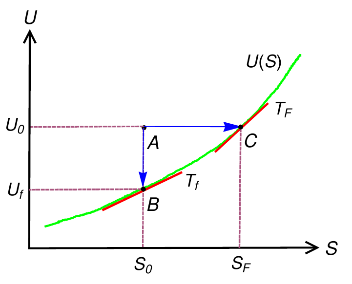
Figure 1: The (green) curve $U(S)$ represents the fundamental relation of the body at equilibrium, at a given volume $V$ and the number of moles $N$. Point $A$ which lies away from this curve, represents the initial, non-equilibrium state. We can go from state $A$ to the equilibrium state $C$ by preserving the initial energy and increasing the entropy of the system, in accordance with the second law. Alternately, we can go from state $A$ to another equilibrium state $B$ by keeping the entropy fixed, but lowering the energy by extracting work. The (red) tangents at points $B$ and $C$ denote the final equilibrium temperatures $T_{f}$ and $T_{F}$, respectively. The convex nature of the $U(S)$ curve (implying $(\partial^{2}U/\partial S^{2})_{V,N}\geq 0$) ensures that $T_{f}<T_{F}$.

III Continuous case: Thermalisation in a rod

We now consider a homogeneous rod of length $L$ whose one end ($x=0$) is in thermal contact with a heat reservoir at temperature $T_{1}$. The other end ($x=L$) is similarly maintained at temperature $T_{2}\;(>T_{1})$. Heat flows from the hot to the cold end. A steady state is achieved in which the temperature profile along the length of the rod is given by a monotonic increasing function $T_{\rm in}(x)$, satisfying $T_{1}\leq T_{\rm in}(x)\leq T_{2}$, where $0\leq x\leq L$. The rod may be regarded as a continuum of elements, each of length $dx$. Accordingly, the sum over index $i$ of the elements, performed in the previous section, may be replaced by an integration over the position variable $x$. The rod, with the initial profile $T_{\rm in}(x)$, is now thermally insulated from the surroundings. There is heat flow between the elements due to their unequal temperatures. After a sufficiently long time, a uniform temperature ($T_{F}$) is obtained along the length of the rod and the flow of heat stops.

Let $C(x,T)>0$ be the heat capacity per unit length at position $x$ of the rod with local temperature $T(x)$. We define a real-valued function of the common temperature $T$ of the rod, given by:

$$\mathscr{Q}(T)=\int_{0}^{L}\!dx\int_{T_{\rm in}(x)}^{T}C(x,z)\,dz.$$ (8)

Physically, it denotes the net heat exchanged by the rod in a process with the final temperature $T$. Since ${d\mathscr{Q}}/{dT}=\int_{0}^{L}C(x,T)dx\;>0$, it implies $\mathscr{Q}$ is an increasing function of $T$. Thus, the function admits only one zero, i.e. $\mathscr{Q}(T_{F})=0$, where $T_{F}$ is a generalized mean temperature, satisfying $T_{1}\leq T_{F}\leq T_{2}$. The condition

$$\mathscr{Q}(T_{F})=\int_{0}^{L}\!dx\int_{T_{\rm in}(x)}^{T_{F}}C(x,z)\,dz=0,$$ (9)

also implies conservation of energy of the rod in an adiabatic process when the work involved is also zero.

Let $\Delta\mathscr{S}(T)$ be another real-valued function, defined as:

$$\Delta\mathscr{S}(T)=\int_{0}^{L}\!dx\int_{T_{\rm in}(x)}^{T}\frac{C(x,z)}{z}\,dz.$$ (10)

Since the temperature is defined to be positive, $\Delta\mathscr{S}(T)$ is also an increasing function of $T$. The function $\Delta\mathscr{S}(T)$ evaluates the entropy change of the total system (rod) from the initial non-equilibrium state to the final equilibrium state at a common temperature $T$. Thus, $\Delta\mathscr{S}(T_{F})$ defines the change in entropy of the rod undergoing adiabatic thermalisation.

Now, since $T_{\rm in}(x)$ is a continuous, monotonic function of $x$, we can define a position $x=r$ with $T_{\rm in}(r)=T_{F}$ such that the elements in the $x$-range $[0,r]$ have their initial temperatures lower than $T_{F}$, while the elements in the range $(r,L]$ are initially at temperatures higher than $T_{F}$. Note that the value $r$ itself depends on the heat capacity function and initial temperature profile. Then, we can write

$$\Delta\mathscr{S}(T_{F})=\int_{0}^{r}\!dx\int_{T_{\rm in}(x)}^{T_{F}}\frac{C(x,z)}{z}\,dz+\int_{r}^{L}\!dx\int_{T_{\rm in}(x)}^{T_{F}}\frac{C(x,z)}{z}\,dz$$ (11)

Thus, the first term above is positive while the second one is negative. Similarly, it is convenient to write Eq. (9) in the following form:

$$\mathscr{Q}(T_{F})=\int_{0}^{r}\!dx\int_{T_{\rm in}(x)}^{T_{F}}C(x,z)\,dz+\int_{r}^{L}\!dx\int_{T_{\rm in}(x)}^{T_{F}}C(x,z)\,dz=0.$$ (12)

Now, invoking the decreasing nature of the function $1/z$, we obtain

$$\int_{0}^{r}\!dx\int_{T_{\rm in}(x)}^{T_{F}}\frac{C(x,z)}{z}dz >\frac{1}{T_{F}}\int_{0}^{r}\!dx\int_{T_{\rm in}(x)}^{T_{F}}C(x,z)dz$$

$$=-\frac{1}{T_{F}}\int_{r}^{L}\!dx\int_{T_{\rm in}(x)}^{T_{F}}C(x,z)dz$$

$$=\frac{1}{T_{F}}\int_{r}^{L}\!dx\int_{T_{F}}^{T_{\rm in}(x)}C(x,z)dz>\int_{r}^{L}\!dx\int_{T_{F}}^{T_{\rm in}(x)}\frac{C(x,z)}{z}dz,$$ (13)

where we used Eq. (12) in the second step above. Thus, we can write Eq. (11) as

$$\Delta\mathscr{S}(T_{F})=\int_{0}^{r}\!dx\int_{T_{\rm in}(x)}^{T_{F}}\frac{C(x,z)}{z}dz-\int_{r}^{L}\!dx\int_{T_{F}}^{T_{\rm in}(x)}\frac{C(x,z)}{z}dz>0,$$ (14)

or

$$\Delta\mathscr{S}(T_{F})=\int_{0}^{L}\!dx\int_{T_{\rm in}(x)}^{T_{F}}\frac{C(x,z)}{z}dz>0.$$ (15)

The above analysis proves that the function $\Delta\mathscr{S}$ evaluated at $T_{F}$ is strictly positive. Since $\Delta\mathscr{S}(T)$ in Eq. (10) is an increasing function, there must exist a unique lower value of the temperature $T_{f}(<T_{F})$ at which the function $\Delta\mathscr{S}(T)$ admits a zero [6]:

$$\Delta\mathscr{S}(T_{f})=\int_{0}^{L}\!dx\int_{T_{\rm in}(x)}^{T_{f}}\frac{C(x,z)}{z}dz=0.$$ (16)

Upon writing $\Delta\mathscr{S}(T_{F})$ in the following form

$$\Delta\mathscr{S}(T_{F})=\int_{0}^{L}\!dx\int_{T_{\rm in}(x)}^{T_{f}}\frac{C(x,z)}{z}dz+\int_{0}^{L}\!dx\int_{T_{f}}^{T_{F}}\frac{C(x,z)}{z}dz>0,$$ (17)

we obtain from Eqs. (16) and (17):

$$\Delta\mathscr{S}(T_{F})=\int_{0}^{L}\!dx\int_{T_{f}}^{T_{F}}\frac{C(x,z)}{z}dz>0.$$ (18)

We recall that $T_{F}$ is evaluated from the energy-conserving condition (9), while $T_{f}$ follows from the entropy-conserving condition (16). The change in internal energy in the first step of the alternate process is extracted in the form of work:

$$\mathscr{W}=\int_{0}^{L}\!dx\int_{T_{\rm in}(x)}^{T_{f}}{C(x,z)}\,dz<0.$$ (19)

The amount of heat added in the second step is given by:

$$\mathscr{Q}^{\prime}=\int_{0}^{L}\!dx\int_{T_{f}}^{T_{F}}C(x,z)\,dz>0.$$ (20)

which by virtue of the condition (9) implies $\mathscr{Q}^{\prime}=-\mathscr{W}$.

III.1 Special case

After demonstarting the Second law inequality in a rod with a general heat capacity function $C(x,T)$ and a monotonic initial profile $T_{\rm in}(x)$, we illustrate our results for a special case. Consider the rod with a constant heat capacity per unit length i.e. $C(x,T)=C$ [9]. First, treating thermalisation as an adiabatic process, the constraint of energy conservation (Eq. (9)) yields:

$$T_{F}=\frac{1}{L}\int_{0}^{L}{T_{\rm in}(x)}dx\equiv\langle T_{\rm in}(x)\rangle,$$ (21)

where $\langle\cdot\cdot\rangle$ denotes the mean value over $x$. The change in the entropy of the rod is evaluated as:

$$\Delta\mathscr{S} =CL\ln T_{F}-C\int_{0}^{L}\ln T_{\rm in}(x)\;dx.$$ (22)

Next, we consider the alternate two-step process. First, a reversible process is done on the rod such that the rod attains the common temperature $T_{f}$. For the rod with a constant heat capacity per unit length ($C$), the entropy conserving condition (Eq. (16)) yields:

$$T_{f}=\exp\langle\ln T_{\rm in}(x)\rangle.$$ (23)

Using the above expression in Eq. (22), we can write:

$$\Delta\mathscr{S}=CL\ln\frac{T_{F}}{T_{f}}>0,$$ (24)

since $T_{F}>T_{f}$, due to the application of Jensen’s inequality: $\ln\langle T_{\rm in}(x)\rangle>\langle\ln T_{\rm in}(x)\rangle$. The amount of work is given by $\mathscr{W}=CL(T_{f}-T_{F})<0$ which is equal in magnitude of the heat added in the second step.

Note that we have not yet assumed any specific form for the initial temperature profile. Following the assumption of a linear temperature profile: $T_{\rm in}(x)=T_{1}+(T_{2}-T_{1})x/L$, we find

$$T_{F}=\frac{T_{2}+T_{1}}{2},\quad T_{f}=\frac{1}{e}\left(\frac{T_{1}^{T_{1}}}{T_{2}^{T_{2}}}\right)^{\frac{1}{T_{1}-T_{2}}}.$$ (25)

The first formula gives the arithmetic mean while the second is known as the Identric mean [7, 8] of two numbers $T_{1}\neq T_{2}>0$. The former is greater than the latter ($T_{F}>T_{f}$), with equality only if $T_{1}=T_{2}$.

Finally, from Eq. (24), the entropy change may be explicitly written in the form:

$$\Delta\mathscr{S}=CL\left(1+\ln T_{F}-\frac{T_{2}\ln T_{2}-T_{1}\ln T_{1}}{T_{2}-T_{1}}\right)>0,$$ (26)

which is also derived in Ref. [1] using the Clausius formula in a thermal adiabatic process.

IV Conclusions

We have considered adiabatic thermalisation of an initially nonequilibrium state of a body to a final equilibrium state at a uniform temperature. The nonequilibrium state may be imagined as consisting of $n$ bodies or parts which are themselves in internal equilibrium, though not in mutual equilibrium with each other. So, we are able to assign equilibrium thermodynamic quantities to different parts in the initial state. For instance, the total entropy of the composite body is the sum of the entropies of individual parts: $S_{\rm in}=\sum_{i=1}^{n}S_{i}$. Similar considerations apply to the continuum case.

Now, the adiabatic process can be alternately visulized as a two-step process. The first step consists of a reversible work extraction by which the body attains a temperature $T_{f}$, followed by the the second step involving addition of heat to the body — equal in magnitude to the extracted work, thus restoring the body to its initial energy. The body attains the same final temperature $T_{F}$ as in the adiabatic process, satisfying $T_{F}>T_{f}$. The entropy change in the adiabatic process is $\Delta S=S(T_{F})-S_{\rm in}$. It is not straightforward to infer that in general entropy should increase in this process. The usual simplification is to assume particular thermodynamic systems and make use of algebraic inequalities to infer $\Delta S>0$, hence validating the second law for those special cases.

Due to the alternate process, we have $S_{\rm in}=S(T_{f})$. Further, owing to the assumption of positive heat capacities for all the different parts of the body, $S(T)$ is a monotonic increasing function. Thereby, $T_{F}>T_{f}$ inequality directly leads to the result $\Delta S=S(T_{F})-S(T_{f})>0$. Thus, we observe here the relevance of positive heat capacities in a more general context (see also Ref. [10]).

In the second step, the added heat is equal in magnitude to the extracted work. This suggests that there are two ways in which this may be accomplished. Either we may add the extracted work in an irreversible manner, thus converting it into an equivalent amount of heat, or we can add heat reversibly, by bringing the body in thermal contact with a series of reservoirs with temperatures ranging from $T_{f}$ to $T_{F}$. Although, the final state obtained for the body is the same in two cases, there is a subtle difference of physics involved which can be instructive for the students. If we add work dissipatively to the body, the entropy of the body rises due to entropy production. On the other hand, if we add heat reversibly, then entropy of the body increases since heat is being directly added. Admittedly, entropy production is an advanced concept. A student of thermodynamics first encounters the concept of entropy change via heat exchange only ($dS=dQ/T$).

In short, during the original adiabatic process, the entropy increase happens due to entropy production whose justifiable explanation can be given via a statistical treatment, using the idea of microstates. For the alternate process considered in this paper, the entropy increase happens, because heat is added to the body which, in our opinion, makes it more intuitive to understand the manifestation of the second law within the framework of equilibrium thermodynamics.

The alternate process we have considered in Fig. 1 is a reversible process. It does not increase the entropy of the universe, although there is rise in the entropy of the body. Thus, even though we achieve the same state for the body itself, the process is reversible, in contrast to the original adiabatic process. This is the second point that a student of thermodynamics must appreciate. Any irreversible process can be made reversible if sufficient resources (in the form of reversible heat engines, series of heat reservoirs and so on) are made available.

AUTHOR DECLARATIONS

Conflict of Interest

The authors have no conflicts to disclose.

References

- Zemansky [1968] M. W. Zemansky, Heat and thermodynamics; an intermediate textbook (McGraw-Hill New York, 1968).
- Pyun [1974] C. W. Pyun, Generalized means: Properties and applications, American Journal of Physics 42, 896 (1974), https://doi.org/10.1119/1.1987886 .
- Leff [1977] H. S. Leff, Multisystem temperature equilibration and the second law, American Journal of Physics 45, 252 (1977), https://doi.org/10.1119/1.11002 .
- [4] J. Anacleto and J. M. Ferreira, Reversible versus irreversible thermalization of two finite blocks, Eur. J. Phys. 37 022001 (2016).
- Johal [2023] R. S. Johal, The law of entropy increase for bodies in mutual thermal contact, American Journal of Physics 91, 79 (2023), https://doi.org/10.1119/5.0124068. Erratum: American Journal of Physics 91, 328 (2023) https://doi.org/10.1119/5.0142510 .
- Cashwell and Everett [1967] E. D. Cashwell and C. J. Everett, The means of order and the laws of thermodynamics, Am. Math. Monthly 74, 271 (1967).
- Stolarsky [1975] K. B. Stolarsky, Generalizations of the logarithmic mean, Math. Mag. 48, 87 (1975).
- [8] J. Sándor, On the identric and logarithmic means. Aeq. Math. 40, 261–270 (1990). https://doi.org/10.1007/BF0211229
- [9] In general, we may consider a heterogenous rod with a temperature independent heat capacity. In that case, . This is analogous to the discrete case with different for each body.
- [10] J. P. Abriata, Comment on a thermodynamic proof of the inequality between arithmetic and geometric mean, Phys. Lett. 71 A (4), 309-310 (1979).