Sampling from the Gibbs measure of the continuous random energy model and the hardness threshold

Abstract

The continuous random energy model (CREM) is a toy model of disordered systems introduced by Bovier and Kurkova in 2004 based on previous work by Derrida and Spohn in the 80s. In a recent paper by Addario-Berry and Maillard, they raised the following question: what is the threshold $\beta_{G}$, at which sampling approximately the Gibbs measure at any inverse temperature $\beta>\beta_{G}$ becomes algorithmically hard? Here, sampling approximately means that the Kullback–Leibler divergence from the output law of the algorithm to the Gibbs measure is of order $o(N)$ with probability approaching $1$, as $N\rightarrow\infty$, and algorithmically hard means that the running time, the numbers of vertices queries by the algorithms, is beyond of polynomial order.

The present work shows that when the covariance function $A$ of the CREM is concave, for all $\beta>0$, a recursive sampling algorithm on a renormalized tree approximates the Gibbs measure with running time of order $O(N^{1+\varepsilon})$. For $A$ non-concave, the present work exhibits a threshold $\beta_{G}<\infty$ such that the following hardness transition occurs: a) For every $\beta\leq\beta_{G}$, the recursive sampling algorithm approximates the Gibbs measure with running time of order $O(N^{1+\varepsilon})$. b) For every $\beta>\beta_{G}$, a hardness result is established for a large class of algorithms. Namely, for any algorithm from this class that samples the Gibbs measure approximately, there exists $z>0$ such that the running time of this algorithm is at least $e^{zN}$ with probability approaching $1$. In other words, it is impossible to sample approximately in polynomial-time the Gibbs measure in this regime.

Additionally, we provide a lower bound of the free energy of the CREM that could hold its own value.

Keywords:

algorithmic hardness; continuous random energy model; Gaussian process; Gibbs measure; Kullback–Leibler divergence; spin glass.

MSC2020 subject classifications:

68Q17, 82D30, 60K35, 60J80.

1 Introduction

The continuous random energy model (CREM) is a toy model of a disordered system in statistical physics, i.e. a model where the Hamiltonian – the function that assigns energies to the states of the system – is itself random. The CREM was introduced by Bovier and Kurkova [9] based on previous work by Derrida and Spohn [13]. Mathematically, the model is defined as follows. For a given integer $N\in\mathbb{N}$, the CREM is a centered Gaussian process $\mathbf{X}=(X_{u})_{u\in\mathbb{T}_{N}}$ indexed by the binary tree $\mathbb{T}_{N}$ of depth $N$ with covariance function

$$\mathbb{E}\left[X_{v}X_{w}\right]=N\cdot A\left(\frac{\absolutevalue{v\wedge w}}{N}\right),\quad\forall v,w\in\mathbb{T}_{N}.$$

Here, $\absolutevalue{v\wedge w}$ is the depth of the most recent common ancestor of $v$ and $w$, and the function $A$ is assumed to be a non-decreasing function defined on an interval $[0,1]$ such that $A(0)=0$ and $A(1)=1$. An essential quantity of this model is the Gibbs measure, which is a probability measure defined on the set of leaves $\partial\mathbb{T}_{N}$ where the weight of $v\in\partial\mathbb{T}_{N}$ is proportional to $e^{\beta X_{v}}$.

The present work consider the sampling problem of the Gibbs measure. We say that a (randomized) algorithm approximates the Gibbs measure if the Kullback–Leibler divergence from the output law of this algorithm to the Gibbs measure is of order $o(N)$ with probability approaching $1$. The present work considers a recursive sampling algorithm that is similar to the one appearing in [1] and [17]. We shows that when the covariance function $A$ of the CREM is concave, for all $\beta>0$, the recursive sampling algorithm approximates the Gibbs measure with running time of order $O(N^{1+\varepsilon})$. Moreover, when $A$ is non-concave, we identify a threshold $\beta_{G}<\infty$ such that the following hardness transition occurs: a) For every $\beta\leq\beta_{G}$, the recursive sampling algorithm approximates the Gibbs measure with running time of order $O(N^{1+\varepsilon})$. b) For every $\beta>\beta_{G}$, we prove a hardness result for a generic class of algorithms. Namely, there exists $\gamma>0$ such that for any algorithm in this class that approximates the Gibbs measure, the running time of this algorithm is at least $e^{\gamma N}$ with probability approaching $1$.

1.1 Definitions and notation

Throughout this paper, we denote by $\mathbb{N}=\{1,2,\cdots\}$ the set of positive integer. For each pair of integers $n$ and $m$ such that $n\leq m$, we denote by $\llbracket n,m\rrbracket$ the set of integers between $n$ and $m$.

Binary tree.

Fixing $N\in\mathbb{N}$, we denote by $\mathbb{T}_{N}=\{\varnothing\}\cup\bigcup_{n=1}^{N}\{0,1\}^{n}$ the binary tree rooted at $\varnothing$. The depth of a vertex $v\in\mathbb{T}_{N}$ is denoted by $\absolutevalue{v}$. For any $v,w\in\mathbb{T}_{N}$, we write $v\leq w$ if $v$ is a prefix of $w$ and write $v<w$ if $v$ is a prefix of $w$ strictly shorter than $w$. In the following, for any $v\in\mathbb{T}_{N}$, we refer to any vertex $w$ with $w\leq v$ as an ancestor of $v$. For any $v\in\mathbb{T}_{N}$ and $n\in\llbracket 0,\absolutevalue{v}\rrbracket$, define $v[n]$ to be the ancestor of $v$ of depth $n$. For all $v,w\in\mathbb{T}_{N}$, we denote by $v\wedge w$ the most recent common ancestor of $v$ and $w$. We denote by $\partial\mathbb{T}_{N}$ the set of leaves of $\mathbb{T}_{N}$, and for any $v\in\mathbb{T}_{N}$, let $\mathbb{T}^{v}_{n}$ be the subtree of $\mathbb{T}_{N}$ rooted at $v$ with depth $n$.

Continuous random energy model.

Let $A$ be a non-decreasing function defined on an interval $[0,1]$ such that $A(0)=0$ and $A(1)=1$. For the sake of this paper, we assume that there exists a bounded Riemann integrable function $a$ such that $A$ for all $t\in[0,1]$,

$$A(t)=\int_{0}^{t}a(s)\differential{s}.$$

We denote by $\hat{A}$ the concave hull of $A$ (see Figure 1) and by $\hat{a}$ the right derivative of $\hat{A}$. Note that the $\hat{A}$ is also equals to the Riemann integral of $\hat{a}$, i.e., for all $t\in[0,1]$,

$$\hat{A}(t)=\int_{0}^{t}\hat{a}(s)\differential{s}.$$

We now introduce the continuous random energy model (CREM). See Figure 1 for an illustration.

Definition 1.1.

Given $N\in\mathbb{N}$, the continuous random energy model (CREM) is a centered Gaussian process $\mathbf{X}=(X_{u})_{u\in\mathbb{T}_{N}}$ indexed by the binary tree $\mathbb{T}_{N}$ of depth $N$ with covariance function

$$\mathbb{E}\left[X_{v}X_{w}\right]=N\cdot A\left(\frac{\absolutevalue{v\wedge w}}{N}\right),\quad\forall v,w\in\mathbb{T}_{N},$$ (1.1)

where $\absolutevalue{v\wedge w}$ is the depth of the most recent common ancestor of $v$ and $w$.

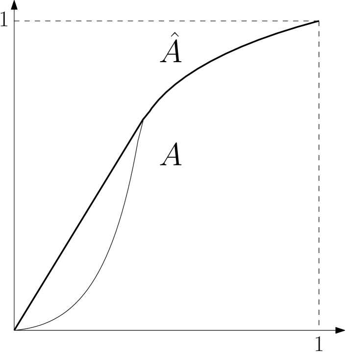
Figure 1: The covariance function of a CREM is determined by the underlying binary tree (left) and a function $A$ (right). The concave hull $\hat{A}$ of the function $A$ is also shown on the right, which determines the CREM free energy and the asymptotics of the maximum of the CREM.

Throughout this paper, we consider a sequence of CREM $(\mathbf{X}_{N})_{N\in\mathbb{N}}$ defined on the same underlying probability space. For simplicity, we drop $N$ as long as it causes no ambiguity.

Branching property.

The CREM can be viewed as an inhomogeneous binary branching random walk with Gaussian increments. In particular, it has the following branching property: let $(\mathscr{F}_{k})_{k=0}^{N}$ be the natural filtration of the CREM. For any $u\in\mathbb{T}_{N}$ with $\absolutevalue{u}=n\in\llbracket 0,N\rrbracket$, call the process

$$\mathbf{X}^{u}=(X^{u}_{w})_{uw\in\mathbb{T}^{u}_{N-n}}$$

the CREM indexed by the subtree $\mathbb{T}^{u}_{N-n}$, where $X^{u}_{w}=X_{uw}-X_{u}$. For any $n\in\llbracket 0,N\rrbracket$, let $\mathbf{X}^{(n)}=(X^{(n)}_{u})_{u\in\mathbb{T}_{N-n}}$ be a centered Gaussian process with covariance function

$$\mathbb{E}\left[X^{(n)}_{w_{1}}X^{(n)}_{w_{2}}\right]=N\cdot A\left(\frac{n+\absolutevalue{w_{1}\wedge w_{2}}}{N}\right),\quad\forall w_{1},w_{2}\in\mathbb{T}_{N-n}.$$

Then, the branching property states that collection of processes $\{\mathbf{X}^{u}:\absolutevalue{u}=n\}$ are independent and have the identical distribution of $\mathbf{X}^{(n)}$, and they are independent of $\mathscr{F}_{n}$.

Partition function and Gibbs measure.

Given a subtree $\mathbb{T}_{M}^{v}$ rooted at $v$ and of depth $M\in\llbracket 0,N-\absolutevalue{v}\rrbracket$, the Gibbs measure with inverse temperature $\beta>0$ is defined by

$$\mu_{\beta,M}^{v}(u)=\frac{1}{Z_{\beta,M}^{v}}e^{\beta X_{u}^{v}},\quad\forall vu\in\mathbb{T}_{M}^{v},$$ (1.2)

where

$$Z_{\beta,M}^{v} =\sum_{vu\in\mathbb{T}_{M}^{v}}e^{\beta X_{u}^{v}},$$ (1.3)

is the partition function on the subtree $\mathbb{T}_{M}^{v}$. In particular, we adopt the conventions

$$\mu_{\beta,M}=\mu_{\beta,M}^{\varnothing}\quad\text{and}\quad Z_{\beta,M}=Z_{\beta,M}^{\varnothing}$$

for any $M\in\llbracket 0,N\rrbracket$. For completeness, we also define $Z^{(n)}_{\beta,M}=\sum_{\absolutevalue{u}=M}e^{\beta X^{(n)}_{u}}$.

Free energy and its lower bound.

For $v\in\mathbb{T}_{N}$, we refer to the logarithm of the partition function $\log Z_{\beta,M}^{v}$ as the free energy on the subtree $\mathbb{T}_{M}^{v}$. The free energy $F_{\beta}$ of the CREM is defined as follows, and $F_{\beta}$ admits an explicit expression.

$$F_{\beta}\coloneqq\lim_{N\rightarrow\infty}\frac{1}{N}\mathbb{E}\left[\log Z_{\beta,N}\right]=\int_{0}^{1}f(\beta\sqrt{\hat{a}(s)})\differential{s},$$ (1.4)

where the function $f$ is defined as

$$f(\beta)=\begin{cases}\displaystyle\log 2+\frac{\beta^{2}}{2},&\beta<\sqrt{2\log 2}\\ \\ \sqrt{2\log 2}\beta,&\beta\geq\sqrt{2\log 2}.\end{cases}$$ (1.5)

For completeness, we include the proof of (1.4) in Fact A.2. When clear, we also simply refer to $F_{\beta}$ as the free energy. We introduce a related quantity $\tilde{F}_{\beta}$ defined as

$$\tilde{F}_{\beta}\coloneqq\int_{0}^{1}f(\beta\sqrt{a(s)})\differential{s}.$$ (1.6)

In Proposition A.1, we show that $F_{\beta}\geq\tilde{F}_{\beta}$ and characterize the condition where the equality holds.

Algorithms.

We follow the same definition of randomized algorithms as in [1, 17], which also appeared in similar forms in [23].

Definition 1.2 (Algorithm).

Let $N\in\mathbb{N}$. Let $\tilde{\mathscr{F}}_{k}$ be a filtration defined by

$$\tilde{\mathscr{F}}_{k}=\sigma\left(v(1),\ldots,v(k);\,X(v(1)),\ldots,X(v(k));\,U_{1},\ldots,U_{k+1}\right)$$

where $(U_{k})_{k\geq 1}$ is a sequence of i.i.d. uniform random variables on $[0,1]$, independent of the continuous random energy model $\mathbf{X}$. A random sequence $\mathrm{v}=(v(k))_{k\geq 0}$ taking values in $\mathbb{T}_{N}$ is called a (randomized) algorithm if $v(0)=\varnothing$ and $v(k+1)$ is $\tilde{\mathscr{F}}_{k}$-measurable for every $k\geq 0$. We further suppose that there exists a stopping time $\tau$ with respect to the filtration $\tilde{\mathscr{F}}$ and such that $v(\tau)\in\partial\mathbb{T}_{N}$. We call $\tau$ the running time and $v(\tau)$ the output of the algorithm. The law of the output is the (random) distribution of $v(\tau)$, conditioned on $\mathbf{X}$.

Remark 1.3.

Roughly speaking, the filtration $\tilde{\mathscr{F}}=(\tilde{\mathscr{F}}_{k})_{k\geq 0}$ contains all the information about everything the algorithm has queried so far, as well as the additional randomness needed to choose the next vertex.

Throughout the paper, the notion of time complexity is given by the following definition.

Definition 1.4 (Time complexity).

Let $(\tau_{N})$ be a sequence of running time corresponds to a sequence of algorithms indexed by $N$. Let $h:\mathbb{N}\rightarrow\mathbb{N}$ be a function. We say that the sequence of running times is of order $O(h(N))$ if almost surely, there exists $N_{0}\in\mathbb{N}$ such that $\tau_{N}\leq h(N)$. We say the running time is of polynomial order if there exists a polynomial $P(N)$ such that almost surely, there exists $N_{0}\in\mathbb{N}$.

Remark 1.5.

In the rest of the paper, when we say that the running time of an algorithm is of order $O(h(N))$, we implicitly assume that there is an underlying sequence of algorithms indexed by $N$, which we also refer to as an algorithm by abuse of notation.

Kullback–Leibler divergence.

Given two probability measures $P$ and $Q$ defined on a discrete space $\Omega$, the Kullback–Leibler divergence (also known as the relative entropy) from $Q$ to $P$ is defined by

$$\mathbf{d}(P\;||\;Q) =\sum_{\omega\in\Omega}P(\omega)\cdot\log\left(\frac{P(\omega)}{Q(\omega)}\right).$$ (1.7)

From now on, we abbreviate the Kullback–Leibler divergence as the KL divergence.

The notion of approximation in the present work is the following.

Definition 1.6.

Let $(P_{N})_{N\in\mathbb{N}}$ and $(Q_{N})_{N\in\mathbb{N}}$ are two sequences of random probability measures defined on a discrete space $\Omega$. We say that the sequence $(P_{N})_{N\in\mathbb{N}}$ approximates the sequence $(Q_{N})_{N\in\mathbb{N}}$ with probability approaching $1$ if

$$\lim_{N\rightarrow\infty}\mathbb{P}\left(\frac{1}{N}\mathbf{d}(P_{N}\;||\;Q_{N})<\varepsilon_{N}\right)=0.$$

Remark 1.7.

Note that Definition 1.6 is equivalent to saying that

$$\frac{1}{N}\mathbf{d}(P_{N}\;||\;Q_{N})\stackrel{{\scriptstyle\mathbb{P}}}{{\rightarrow}}0,\quad\text{as $N\rightarrow\infty$.}$$

1.2 Main results

Recall that $a$ is the derivative of $A$. By the Lebesgue criterion of Riemann integrability, the function $a$ is continuous almost everywhere on $[0,1]$. If $A$ is non-concave, define the threshold

$$\beta_{G}=\frac{\sqrt{2\log 2}}{\operatorname*{ess\,sup}_{t\in\{A\neq\hat{A}\}}\sqrt{a(t)}},$$ (1.8)

For completeness, we define $\beta_{G}=\infty$ when $A$ is concave. We now state the main results.

1.2.1 Subcritical and critical regime $\beta\leq\beta_{G}$: optimality of recursive sampling

Fix $\beta>0$, $N\in\mathbb{N}$, and $M=M_{N}\in\llbracket 1,N\rrbracket$. Given a configuration of the continuous random energy model with depth $N$, consider the following algorithm:

set $v=\varnothing$ while $\absolutevalue{v}<N$ do

       sample $w$ with $\absolutevalue{w}=M\wedge(N-\absolutevalue{v})$ according to the Gibbs measure $\mu^{v}_{\beta,M\wedge(N-\absolutevalue{v})}$ replace $v$ with $vw$ 

output $v$

Algorithm 1 Recursive sampling on renormalized tree

Remark 1.8.

This is the same algorithm as the one in [17] except that now the law of the Gibbs measure $\mu^{v}_{\beta,M\wedge(N-\absolutevalue{v})}$ depends on the depth of $v$. Again, its running time is deterministic and bounded by $\lceil N/M\rceil 2^{M}$. The output law of Algorithm 1 is a random probability measure $\mu_{\beta,M,N}$ on $\partial\mathbb{T}_{N}$ that is recursively defined as follows:

$$\begin{split}\mu_{\beta,M,0}(\varnothing)&=1\\ \mu_{\beta,M,N\wedge(k+1)M}(vw)&=\mu_{\beta,M,kM}(v)\cdot\mu^{v}_{\beta,M\wedge(N-kM)}(w)\end{split}$$ (1.9)

for all $\absolutevalue{v}=kM$, $\absolutevalue{w}=M\wedge(N-kM)$ and $k\in\llbracket 0,\left\lfloor\frac{N}{M}\right\rfloor\rrbracket$. It is not hard to see that

$$\mu_{\beta,M,N}(u)=\frac{e^{\beta X_{u}}}{Z_{\beta,M,N}(u)},$$ (1.10)

where

$$Z_{\beta,M,N}(u)=\prod_{k=1}^{\lfloor N/M\rfloor}Z_{\beta,M\wedge(N-kM)}^{u[kM]}.$$

The first theorem states that the KL divergence from the output law of Algorithm 1 to the Gibbs measure concentrates in the following sense.

Theorem 1.9 (Concentration bounds).

Let $\beta>0$, $N\in\mathbb{N}$ and $M\in\llbracket 1,N\rrbracket$. Then for all $p\geq 1$, there exists a constant $C_{p}>0$ depending only on $p$ such that

$$\frac{1}{N}\norm{\mathbf{d}(\mu_{\beta,M,N}\;||\;\mu_{\beta,N})-\mathbb{E}\left[\mathbf{d}(\mu_{\beta,M,N}\;||\;\mu_{\beta,N})\right]}_{p}\leq\frac{\beta C_{p}}{\sqrt{M}}.$$

Next, we show that with a suitable choice of $M_{N}$, the expectation of the KL divergence renormalized by $N$ converges to the difference between $F_{\beta}$ and $\tilde{F}_{\beta}$.

Theorem 1.10 (Convergence of the KL divergence).

Let $\beta>0$, $N\in\mathbb{N}$, and $M_{N}$ be a sequence such that $M_{N}\in\llbracket 1,N\rrbracket$ and $M_{N}\rightarrow\infty$. Let $\tilde{\mu}_{\beta,N}=\mu_{\beta,M_{N},N}$ be the output law of Algorithm 1. Then,

$$\lim_{N\rightarrow\infty}\frac{1}{N}\mathbb{E}\left[\mathbf{d}(\tilde{\mu}_{\beta,N}\;||\;\mu_{\beta,N})\right]=F_{\beta}-\tilde{F}_{\beta}\geq 0,$$

with equality holding if and only if $\beta\leq\beta_{G}$.

As a corollary of Theorem 1.10, in the subcritical regime, with a good choice of $M_{N}$, the mean of the KL divergence divided by $N$ converges to $0$ when $N\rightarrow\infty$. Moreover, for $\varepsilon>0$, with a good choice of $M_{N}$, the running time is of $O(N^{1+\varepsilon})$.

Corollary 1.11 (Efficient sampling).

Fix $\beta\in[0,\beta_{G}]$. Given $\varepsilon>0$, let $M_{N}=\lfloor\varepsilon\log_{2}N\rfloor\wedge N$ and $\tilde{\mu}_{\beta,N}=\mu_{\beta,M_{N},N}$ be the output law of Algorithm 1. Then,

$$\lim_{N\rightarrow\infty}\frac{1}{N}\mathbb{E}\left[\mathbf{d}(\tilde{\mu}_{\beta,N}\;||\;\mu_{\beta,N})\right]=0.$$ (1.11)

Moreover, the running time is deterministic and of order $O(N^{1+\varepsilon})$.

Remark 1.12.

Note that for $A$ concave, Corollary 1.11 yields that Algorithm 1 approximates the Gibbs measure for all $\beta\in(0,\infty)$ as $\beta_{G}=\infty$ for $A$ concave.

Corollary 1.11 implies in particular that the algorithm approximates the Gibbs measure with probability approaching $1$. Indeed, if we choose, e.g., $\varepsilon_{N}=(\frac{1}{N}\mathbb{E}\left[\mathbf{d}(\tilde{\mu}_{\beta,N}\;||\;\mu_{\beta,N})\right])^{1/2}$, Corollary 1.11 and Markov’s inequality then yield

$$\mathbb{P}\left(\frac{1}{N}\mathbf{d}(\tilde{\mu}_{\beta,N}\;||\;\mu_{\beta,N})\leq\varepsilon_{N}\right)\geq 1-\varepsilon_{N}^{1/2}\rightarrow 1,\quad\text{as}\quad N\rightarrow\infty.$$ (1.12)

We provide the proof of Corollary 1.11 below as it is short.

Proof of Corollary 1.11.

Note that the choice of $M_{N}$ satisfies the assumption of Theorem 1.10, so the first statement follows directly from Theorem 1.10. Next, as mentioned in Remark 1.8, the running time of Algorithm 1 is deterministic and is bounded by $\lceil N/M_{N}\rceil 2^{M_{N}}$. With our choice of $M_{N}$, we conclude that

$$\lceil N/M_{N}\rceil 2^{M_{N}}\leq N\cdot 2^{\varepsilon\log_{2}N}\leq N^{1+\varepsilon},$$

and the proof is completed. ∎

1.2.2 Supercritical regime $\beta>\beta_{G}$: hardness for generic algorithms

Now we assume that $A$ is non-concave, so $\beta_{G}<\infty$. For $\beta>\beta_{G}$, we provide the following hardness result for the class of algorithms satisfying Definition 1.2.

Theorem 1.13 (Hardness).

Suppose that $A$ is non-concave. Let $\beta>\beta_{G}$. For any algorithm satisfying Definition 1.2 that approximates the Gibbs measure with probability approaching $1$, there exists $\gamma>0$ such that

$$\lim_{N\rightarrow\infty}\mathbb{P}\left(\tau\geq e^{\gamma N}\right)=1,$$

where $\tau$ is the running time of the algorithm.

1.3 Discussion and related work

A natural way to sample from the Gibbs measure is via the Markov chain Monte Carlo (MCMC) method. In [21], Nascimento and Fontes studied a Metropolis dynamics on the GREM, where the state space of this dynamics is the set of leaves. They showed that for all $\beta>0$, the spectral gap of the Metropolis dynamics decays exponentially to $0$ as $N\rightarrow\infty$ almost surely, which hinted that the MCMC method might not be the best way to approximate the Gibbs measure efficiently.

The current work is largely inspired by the previous work of Addario-Berry and Maillard [1] on finding the near maximum (ground state) of the CREM. Bovier and Kurkova showed in [9] that the maximum of the CREM satisfies

$$x_{GSE}\coloneqq\lim_{N\rightarrow\infty}\frac{1}{N}\mathbb{E}\left[\max_{\absolutevalue{u}=N}X_{u}\right]=\sqrt{2\log 2}\int_{0}^{1}\sqrt{\hat{a}(s)}\differential{s}.$$ (1.13)

With this result in mind, the problem that Addario-Berry and Maillard addressed can be phrased as the following optimization problem.

Problem 1.14.

For what kind of $A$ such that for all $\varepsilon>0$, there exists a polynomial-time algorithm that can find a vertex $\absolutevalue{u}=N$ such that $X_{u}\geq(x_{GSE}-\varepsilon)N$ with high probability?

To respond to Problem 1.14, they showed the following phase transition: there exists a threshold

$$x_{*}=\sqrt{2\log 2}\int_{0}^{1}\sqrt{a(s)}\differential{s}$$

such that for any $x<x_{*}$, there exists a linear time algorithm that finds $X_{v}\geq xN$ with high probability; for any $x>x_{*}$, there exists $z>0$ such that with high probability, it takes at least $e^{zN}$ queries to find $X_{u}\geq xN$. Since $x_{GSE}\geq x_{*}$ with equality holding if and only if $A$ is concave, the near maximum can be found if and only if $A$ is concave. Another remark is that their result correspond to the special case of our result where $\beta\rightarrow\infty$, and linear algorithm they proposed is similar to Algorithm 1.

Problem 1.14 also appeared in the context of mean-field spin glass. It is known that a generalized Thouless–Anderson–Palmer approach proposed by Subag in [27] gives a tree structure from the origin to the spin space when $\beta=\infty$. This picture allows Subag to show in [26] that for the full-RSB spherical spin glasses, a greedy type algorithm that exploits this tree structure gives an efficient way to find a near maximum of these models. On the other hand, it was conjectured by the physicists that when $\beta\rightarrow\infty$, the SK model also exhibits the full-RSB property (see [19]). By assuming this conjecture, Montanari solved Problem 1.14 for the SK model in [20] via the so-called approximate message passing (AMP) type algorithm, where one example of the AMP algorithms was Bolthausen’s iteration scheme [7] which solves the so-called TAP equation. Later, Alaoui, Montanari and Sellke [2] extended Montanari’s previous result to other mean-field spin glasses that do not exhibit the overlap gap property.

The problem of sampling from the Gibbs measure was also considered the context of mean-field spin glasses. This problem was usually attacked by introducing the Glauber dynamics, which also belongs to the MCMC method. For the Sherrington–Kirkpatrick model, physicists (see [25, 19]) expected fast convergence to the Gibbs measure in the whole high temperature regime $\beta<1$. Recently, it was shown by Bauerschmidt and Bodineau in [5] and by Eldan, Koehler and Zeitouni in [14] that fast mixing occurs when $\beta<1/4$. Moreover, Eldan et al. showed in [14] that the Gibbs measure satisfies a Poincaré inequality for the Dirichlet form of Glauber dynamics, so the Glauber dynamics mixes in $O(N^{2})$ spin flips in total variation distance. Subsequently, this estimate was improved to $O(N\log N)$ by Anari et al. in [4].

For spherical spin glasses, Gheissari and Jagannath in [16] that Langevin dynamics (continuum version of Glauber dynamics) have a polynomial spectral gap for $\beta$ small. On the other hand, Ben Arous and Jagannath proved in [6] that for $\beta$ sufficiently large, the mixing times of Glauber and Langevin dynamics are exponentially large in Ising and spherical spin glasses, respectively.

In [3], Alaoui, Montanari and Sellke proposed a non MCMC type algorithm based on the stochastic localization for the SK model. They showed that for $\beta<1/2$, there exists an algorithm with complexity $O(N^{2})$ with output law being close to the Gibbs measure in normalized Wasserstein distance. Moreover, for $\beta>1$, they established a hardness result for the stable algorithms, which means that the output law of these algorithms are stable under small random perturbation of the defining matrix of the SK model. The hardness result for $\beta>1$ was proven by utilizing the disorder chaos, which means for them that Wasserstein distance between the Gibbs measure and the perturbed Gibbs measure is bounded from below by a positive constant for arbitrary small random perturbation.

Overlap gap property and algorithmic hardness.

The overlap gap property, emerging from studying of mean-field spin glasses, seems to be an obstruction of many optimization algorithms for random structures. See Gamarnik [15] for a survey. In the context of the CREM, for a given $\beta>0$, the overlap distribution is the limiting law (as $N\to\infty$) of the overlap $\frac{\absolutevalue{u\wedge w}}{N}$ of two vertices $u$ and $w$ sampled independently according to the Gibbs measure with inverse temperature $\beta$. The CDF of the limiting overlap distribution $\alpha_{\beta}:[0,1]\rightarrow[0,1]$ is defined as

$$\alpha_{\beta}(t)\coloneqq\lim_{N\rightarrow\infty}\mathbb{E}\left[\sum_{\absolutevalue{u}=N}\sum_{\absolutevalue{w}=N}\mu_{\beta,N}(u)\mu_{\beta,N}(w)\boldsymbol{1}_{\absolutevalue{u\wedge w}/N\leq t}\right],$$

The overlap gap property in the context of the CREM means that $\alpha_{\beta}(t)$ is equal to a constant strictly less than $1$ in an interval $[t_{1},t_{2}]\subseteq[0,1]$. On the other hand, it is known in [9] that $\alpha_{\beta}(t)$ satisfies the following

$$\alpha_{\beta}(t)=\begin{cases}\displaystyle\frac{\sqrt{2\log 2}}{\beta\sqrt{\hat{a}(t)}},&t\leq t_{0}(\beta),\\ \\ 1,&t>t_{0}(\beta).\end{cases}$$

When $A$ is concave, the CREM does not exhibits the overlap gap property for any $\beta>0$, which does not contradict the picture mentioned in the previous paragraph. On the other hand, when $A$ is non-concave, the CREM has the overlap gap property if and only if $\beta>\beta_{G}^{\prime}=\sqrt{2\log 2}/\sqrt{\hat{a}(t_{G})}$. Comparing with the hardness threshold $\beta_{G}$ defined in (1.8), we see $\beta_{G}<\beta_{G}^{\prime}$, which means that some extra ingredients are needed to explain the algorithmic hardness we observe in the present work.

Further direction.

Corollary 1.11 implies that if $A$ is concave, for any $\beta\in[0,\infty)$, then the sequence of algorithm constructed from Algorithm 1 can approximate the Gibbs measure in the sense of Definition 1.6. One might ask whether a higher precision is achievable. Namely, let $\alpha\in[0,1)$. Given $\beta>0$, does there exist a sequence of algorithms with corresponding output laws $\tilde{\mu}_{\beta,N}$ such that

$$\lim_{N\rightarrow\infty}\frac{1}{N^{\alpha}}\mathbf{d}(\tilde{\mu}_{\beta,N}\;||\;\mu_{\beta,N})=0,$$

with probability approaching $1$? Note that for a general class of branching random walks, with $\alpha=0$ and $\beta>\beta_{c}$, it is shown in [17] that with positive probability, this task has a running time of stretched exponential. The result in [17] is derived from the fluctuation of the sampled path of supercritical Gibbs measure done by [12].

Outline.

The paper is organized as follows. In Section 2, we prove that the KL divergence $\mathbf{d}(\mu_{\beta,M,N}\;||\;\mu_{\beta,N})$ can be decomposed into weight sums of free energies on subtrees, and we also compute its expectation. This information readily allows us to prove Theorem 1.9 which is provided in Section 2.1. Building on the decomposition of the KL divergence provided in Section 2.1, we study in Section 3 the renormalized limit of $\mathbb{E}\left[\mathbf{d}(\mu_{\beta,M,N}\;||\;\mu_{\beta,N})\right]$. This leads to the proof of Theorem 1.10 which is provided at the end of the introduction of Section 3. In Section 4, we show that for $A$ non-concave and $\beta>\beta_{G}$, the Gibbs measure tends to sample a rare event. Based on this observation, Theorem 1.13 is proven in Section 5, where the details are provided at the end of the introduction of Section 5. In Appendix A, we provide a lower bound of the free energy $F_{\beta}$ that may be of independent interest. Finally, in Appendix B, we provide the details of the proof of Lemma 3.2.

2 Decomposition of the KL divergence $\mathbf{d}(\mu_{\beta,M,N}\;||\;\mu_{\beta,N})$

In this section, we provide in the following proposition a simple decomposition of the KL divergence $\mathbf{d}(\mu_{\beta,M,N}\;||\;\mu_{\beta,N})$ in terms of a sum of free energies on subtrees.

Proposition 2.1.

For all $\beta>0$ and for any two integers $M,N\in\mathbb{N}$ such that $M\leq N$, we have

$$\mathbf{d}(\mu_{\beta,M,N}\;||\;\mu_{\beta,N})=\log Z_{\beta,N}-\sum_{k=0}^{\lfloor N/M\rfloor}\sum_{\absolutevalue{u}=kM}\mu_{\beta,M,kM}(u)\cdot\log Z^{u}_{\beta,M\wedge(N-kM)}.$$

Proof.

By (1.7) the definition of the KL divergence,

$$\mathbf{d}(\mu_{\beta,M,N}\;||\;\mu_{\beta,N})$$

$$=\sum_{\absolutevalue{u}=N}\mu_{\beta,M,N}(u)\cdot(\log Z_{\beta,N}-\log Z_{\beta,M,N}(u))$$ (By (1.2) and (1.10))

$$=\sum_{\absolutevalue{u}=N}\mu_{\beta,M,N}(u)\cdot\Big{(}\log Z_{\beta,N}-\sum_{k=0}^{\lfloor N/M\rfloor}\log Z^{u[kM]}_{\beta,M\wedge(N-kM)}\Big{)}$$

$$=\log Z_{\beta,N}-\sum_{\absolutevalue{u}=N}\sum_{k=0}^{\lfloor N/M\rfloor}\mu_{\beta,M,N}(u)\cdot\log Z^{u[kM]}_{\beta,M\wedge(N-kM)}$$

$$=\log Z_{\beta,N}-\sum_{k=0}^{\lfloor N/M\rfloor}\sum_{\absolutevalue{u}=N}\mu_{\beta,M,N}(u)\cdot\log Z^{u[kM]}_{\beta,M\wedge(N-kM)}$$

$$=\log Z_{\beta,N}-\sum_{k=0}^{\lfloor N/M\rfloor}\sum_{\absolutevalue{w}=kM}\sum_{\absolutevalue{w^{\prime}}=N-kM}\mu_{\beta,M,N}(ww^{\prime})\cdot\log Z^{w}_{\beta,M\wedge(N-kM)}$$

$$=\log Z_{\beta,N}-\sum_{k=0}^{\lfloor N/M\rfloor}\sum_{\absolutevalue{w}=kM}\mu_{\beta,M,kM}(w)\cdot\log Z^{w}_{\beta,M\wedge(N-kM)},$$ (By (1.9))

the proof is completed. ∎

The next proposition asserts that the expectation of the KL divergence $\mathbf{d}(\mu_{\beta,M,N}\;||\;\mu_{\beta,N})$ can be written as the difference between the free energy of the CREM and the sum of free energies on the subtrees.

Proposition 2.2.

For all $\beta>0$ and for any two integers $M,N\in\mathbb{N}$ such that $M\leq N$, the expectation of the KL divergence from $\mu_{\beta,M,N}$ to $\mu_{\beta,N}$ admits the following decomposition.

$$\mathbb{E}\left[\mathbf{d}(\mu_{\beta,M,N}\;||\;\mu_{\beta,N})\right]=\mathbb{E}\left[\log Z_{\beta,N}\right]-\sum_{k=1}^{\lfloor N/M\rfloor}\mathbb{E}\left[\log Z^{(kM)}_{\beta,M\wedge(N-kM)}\right].$$

Proof.

Combining Proposition 2.1, the branching property and the law of iterated expectation, we have

$$\mathbb{E}\left[\mathbf{d}(\mu_{\beta,M,N}\;||\;\mu_{\beta,N})\right]$$

$$=\mathbb{E}\left[\log Z_{\beta,N}\right]-\mathbb{E}\left[\sum_{k=0}^{\lfloor N/M\rfloor}\sum_{\absolutevalue{u}=kM}\mu_{\beta,M,kM}(u)\cdot\log Z^{u}_{\beta,M\wedge(N-kM)}\right]$$

$$=\mathbb{E}\left[\log Z_{\beta,N}\right]-\mathbb{E}\left[\sum_{k=0}^{\lfloor N/M\rfloor}\sum_{\absolutevalue{u}=kM}\mu_{\beta,M,kM}(u)\cdot\mathbb{E}\left[\log Z^{u}_{\beta,M\wedge(N-kM)}\,\middle|\,\mathscr{F}_{kM}\right]\right]$$

$$=\mathbb{E}\left[\log Z_{\beta,N}\right]-\sum_{k=0}^{\lfloor N/M\rfloor}\mathbb{E}\left[\sum_{\absolutevalue{u}=kM}\mu_{\beta,M,kM}(u)\right]\mathbb{E}\left[\log Z^{(kM)}_{\beta,M\wedge(N-kM)}\right]$$

$$=\mathbb{E}\left[\log Z_{\beta,N}\right]-\sum_{k=0}^{\lfloor N/M\rfloor}\mathbb{E}\left[\log Z^{(kM)}_{\beta,M\wedge(N-kM)}\right],$$ (2.1)

where (2.1) follows from the fact that $\mu_{\beta,M,kM}$ is a probability measure. ∎

2.1 Proof of Theorem 1.9

The following argument is similar to the proof of (1.9) in [17], where the difference is that we use the concentration inequalities of free energies to control certain terms.

Let $p\geq 1$. By Proposition 2.1 and Minkowski’s inequality, we have

$$\frac{1}{N}\norm{\mathbf{d}(\mu_{\beta,M,N}\;||\;\mu_{\beta,N})-\mathbb{E}\left[\mathbf{d}(\mu_{\beta,M,N}\;||\;\mu_{\beta,N})\right]}_{p}$$

$$\leq\frac{1}{N}\sum_{k=0}^{\lfloor N/M\rfloor}\norm{\sum_{\absolutevalue{u}=kM}\mu_{\beta,M,kM}(u)\cdot\left(\log Z^{u}_{\beta,M\wedge(N-kM)}-\mathbb{E}\left[\log Z^{u}_{\beta,M\wedge(N-kM)}\right]\right)}_{p}.$$ (2.2)

Applying Jensen’s inequality to $\mu_{\beta,M,kM}$ and the fact that $x\mapsto\absolutevalue{x}^{p}$ is convex for all $p\geq 1$, we obtain

$$\mathbb{E}\left[\absolutevalue{\sum_{\absolutevalue{u}=kM}\mu_{\beta,M,kM}(u)\cdot\left(\log Z^{u}_{\beta,M\wedge(N-kM)}-\mathbb{E}\left[\log Z^{u}_{\beta,M\wedge(N-kM)}\right]\right)}^{p}\right]$$

$$\leq\mathbb{E}\left[\sum_{\absolutevalue{u}=kM}\mu_{\beta,M,kM}(u)\cdot\absolutevalue{\log Z^{u}_{\beta,M\wedge(N-kM)}-\mathbb{E}\left[\log Z^{u}_{\beta,M\wedge(N-kM)}\right]}^{p}\right].$$ (2.3)

Then by the law of iterated expectation and the branching property, the expectation (2.3) above equals

$$\mathbb{E}\left[\sum_{\absolutevalue{u}=kM}\mu_{\beta,M,kM}(u)\cdot\mathbb{E}\left[\absolutevalue{\log Z^{u}_{\beta,M\wedge(N-kM)}-\mathbb{E}\left[\log Z^{u}_{\beta,M\wedge(N-kM)}\right]}^{p}\,\middle|\,\mathscr{F}_{kM}\right]\right]$$

$$=\mathbb{E}\left[\absolutevalue{\log Z^{(kM)}_{\beta,M\wedge(N-kM)}-\mathbb{E}\left[\log Z^{(kM)}_{\beta,M\wedge(N-kM)}\right]}^{p}\right].$$ (2.4)

Now, the concentration inequality of free energies (see, Theorem 1.2 in [22]) implies that for all $p\geq 1$,

$$\mathbb{E}\left[\absolutevalue{\log Z^{(kM)}_{\beta,M\wedge(N-kM)}-\mathbb{E}\left[\log Z^{(kM)}_{\beta,M\wedge(N-kM)}\right]}^{p}\right]$$

$$\leq\int_{0}^{\infty}2\exp(-\frac{x^{2/p}}{4\beta^{2}N\Big{(}A\left(\frac{kM+M\wedge(N-kM)}{N}\right)-A\left(\frac{kM}{N}\right)\Big{)}})\differential{x}$$

$$=\beta^{p}N^{p/2}\left(A\left(\frac{kM+M\wedge(N-kM)}{N}\right)-A\left(\frac{kM}{N}\right)\right)^{p/2}\cdot\underbrace{2^{p/2+1}p\int_{0}^{\infty}\exp(-\frac{y^{2}}{2})y^{p-1}\differential{y}}_{\eqqcolon C_{1}(p)}$$

$$=\beta^{p}N^{p/2}\left(A\left(\frac{kM+M\wedge(N-kM)}{N}\right)-A\left(\frac{kM}{N}\right)\right)^{p/2}\cdot C_{1}(p).$$ (2.5)

Combining (2.2), (2.4) and (2.5) and letting $C_{2}(p)=C_{1}(p)^{1/p}$, we derive that

$$\frac{1}{N}\norm{\mathbf{d}(\mu_{\beta,M,N}\;||\;\mu_{\beta,N})-\mathbb{E}\left[\mathbf{d}(\mu_{\beta,M,N}\;||\;\mu_{\beta,N})\right]}_{p}$$

$$\leq\frac{\beta C_{2}(p)}{\sqrt{N}}\sum_{k=0}^{\lfloor N/M\rfloor}\sqrt{\Big{(}A\left(\frac{kM+M\wedge(N-kM)}{N}\right)-A\left(\frac{kM}{N}\right)\Big{)}}$$

$$\leq\frac{\beta C_{2}(p)}{\sqrt{N}}\sqrt{\underbrace{\sum_{k=0}^{\lfloor N/M\rfloor}\left(A\left(\frac{kM+M\wedge(N-kM)}{N}\right)-A\left(\frac{kM}{N}\right)\right)}_{=1}}\sqrt{\sum_{k=0}^{\lfloor N/M\rfloor}1}$$ (2.6)

$$=\frac{\beta C_{2}(p)}{\sqrt{N}}\sqrt{\left\lceil\frac{N}{M}\right\rceil}$$

$$\leq\frac{\beta C_{2}(p)\sqrt{2}}{\sqrt{M}},$$ (2.7)

where (2.6) is derived from the Cauchy–Schwarz inequality, and (2.7) follows from bounding $\sqrt{\lfloor N/M\rfloor/N}$ by $\sqrt{2/M}$. By choosing $C_{p}=C_{2}(p)\sqrt{2}$, the proof of Theorem 1.9 is completed.

3 Asymptotics of the KL divergence $\mathbf{d}(\mu_{\beta,M,N}\;||\;\mu_{\beta,N})$

The goal of this section is to prove Theorem 1.10. In view of (1.4) and Proposition 2.2, it remains to show the following proposition.

Proposition 3.1.

Let $M_{N}$ be a sequence such that $M_{N}\in\llbracket 1,N\rrbracket$ and $M_{N}\rightarrow\infty$. Then,

$$\lim_{N\rightarrow\infty}\frac{1}{N}\sum_{k=1}^{\lfloor N/M_{N}\rfloor}\mathbb{E}\left[\log Z^{(kM_{N})}_{\beta,M_{N}\wedge(N-kM_{N})}\right]=\tilde{F}_{\beta}.$$

The proof of Proposition 3.1 is postponed to Section 3.1. Conditioned on Proposition 3.1, we are now ready to prove Theorem 1.10.

Proof of Proposition 1.10.

Fix $\beta<\beta_{G}$. Let $M_{N}$ be a sequence such that $M_{N}\in\llbracket 1,N\rrbracket$, and $M_{N}\rightarrow\infty$. By Fact A.2 and Proposition 3.1,

$$\lim_{N\rightarrow\infty}\frac{1}{N}\mathbb{E}\left[\mathbf{d}(\mu_{\beta,M_{N},N}\;||\;\mu_{\beta,N})\right] =\lim_{N\rightarrow\infty}\frac{1}{N}\mathbb{E}\left[\log Z_{\beta,N}\right]-\lim_{N\rightarrow\infty}\frac{1}{N}\sum_{k=1}^{\lfloor N/M_{N}\rfloor}\mathbb{E}\left[\log Z^{(kM_{N})}_{\beta,M_{N}\wedge(N-kM_{N})}\right]$$

$$=F_{\beta}-\tilde{F}_{\beta}.$$

Now, by Proposition A.1, $F_{\beta}-\tilde{F}_{\beta}=0$ for all $\beta\leq\beta_{G}$ and $F_{\beta}-\tilde{F}_{\beta}>0$ for all $\beta>\beta_{G}$. This completes the proof. ∎

3.1 Proof of Proposition 3.1

The proof of Proposition 3.1 is based on the following lemma.

Lemma 3.2.

Let $M_{N}$ be a sequence such that $M_{N}\in\llbracket 1,N\rrbracket$ and $M_{N}\rightarrow\infty$. For all $k\in\llbracket 0,\lfloor N/M_{N}\rfloor\rrbracket$, define

$$a_{k}^{-}\coloneqq\operatorname*{ess\,inf}_{t\in[\frac{kM_{N}}{N},\frac{(k+1)M_{N}}{N}]}a(t)\quad\text{and}\quad a_{k}^{+}\coloneqq\operatorname*{ess\,sup}_{t\in[\frac{kM_{N}}{N},\frac{(k+1)M_{N}}{N}]}a(t).$$ (3.1)

Then for all $\varepsilon>0$, there exists $N_{0}\in\mathbb{N}$ such that for all $N\geq N_{0}$,

$$f(\beta\sqrt{a}^{-}_{k})-\varepsilon\beta\sqrt{a}^{-}_{k}\leq\frac{1}{M_{N}}\mathbb{E}\left[\log Z^{(kM)}_{\beta,M}\right]\leq f(\beta\sqrt{a}^{+}_{k})+\varepsilon\beta\sqrt{a}^{+}_{k},$$

for all $k\in\llbracket 0,\lfloor N/M_{N}\rfloor\rrbracket$.

The proof of Lemma 3.2 is based on comparing the free energy of the CREM with the free energy of the so-called branching random walk, which is a CREM with $A$ equal to the identity function. While the proof of Lemma 3.2 is rather standard, the proof requires some standard properties of the free energy of the branching random walk, so we postpone the proof of Lemma 3.2 to Appendix B.

We now proceed to the proof of Proposition 3.1.

Proof of Proposition 3.1.

Fix $\varepsilon>0$. Fix $M_{N}$ being a sequence such that $M_{N}\in\llbracket 1,N\rrbracket$ and $M_{N}\rightarrow\infty$. We denote $K_{N}=\lfloor N/M_{N}\rfloor$ for simplicity. First of all, note that

$$\frac{1}{N}\sum_{k=1}^{K_{N}}\mathbb{E}\left[\log Z_{\beta,M_{N}}^{(kM_{N})}\right]=\frac{1}{N}\sum_{k=1}^{K_{N}-1}\mathbb{E}\left[\log Z_{\beta,M_{N}}^{(kM_{N})}\right]+\frac{1}{N}\mathbb{E}\left[\log Z_{\beta,N-K_{N}M_{N}}^{(K_{N}M_{N})}\right].$$ (3.2)

We claim that the second term of (3.2) converges to $0$. For any $\absolutevalue{u}=N-\lfloor N/M_{N}\rfloor M_{N}$,

$$\mathbb{E}\left[\log Z_{\beta,N-\lfloor N/M_{N}\rfloor M_{N}}^{(\lfloor N/M_{N}\rfloor M_{N})}\right]\geq\mathbb{E}\left[\beta X_{u}^{(\lfloor N/M_{N}\rfloor M_{N})}\right]=0.$$

Now, we turn to the upper bound. By Jensen’s inequality,

$$\frac{1}{N}\mathbb{E}\left[\log Z_{\beta,N-\lfloor N/M_{N}\rfloor M_{N}}^{\lfloor N/M_{N}\rfloor M_{N}}\right] \leq\frac{1}{N}\log\mathbb{E}\left[Z_{\beta,N-\lfloor N/M_{N}\rfloor M_{N}}^{(\lfloor N/M_{N}\rfloor M_{N})}\right]$$

$$=\log 2\left(1-\left\lfloor\frac{N}{M_{N}}\right\rfloor\frac{M_{N}}{N}\right)+\left(A(1)-A\left(\left\lfloor\frac{N}{M_{N}}\right\rfloor\frac{M_{N}}{N}\right)\right)\rightarrow 0,$$

as $N\rightarrow\infty$, which proves that the second term of (3.2) converges to $0$.

It remains to show that the first term of (3.2) converges to $\tilde{F}_{\beta}$. By Lemma 3.2,

$$\frac{M_{N}}{N}\sum_{k=1}^{K_{N}-1}f(\beta\sqrt{a}^{-}_{k})-\varepsilon\beta\sqrt{a}^{-}_{k}\leq\frac{1}{N}\sum_{k=1}^{K_{N}-1}\mathbb{E}\left[\log Z^{(kM)}_{\beta,M}\right]\leq\frac{M_{N}}{N}\sum_{k=1}^{K_{N}-1}f(\beta\sqrt{a}^{+}_{k})+\varepsilon\beta\sqrt{a}^{+}_{k}.$$ (3.3)

Because the function $a(\cdot)$ is Riemann integrable and $f(\beta\sqrt{\cdot})$ is continuous, their composition $f(\beta\sqrt{a(\cdot)})$ is also Riemann integrable. Similarly, $\sqrt{a(\cdot)}$ is also Riemann integrable. Thus, by taking $N\rightarrow\infty$, (3.3) yields

$$\lim_{N\rightarrow\infty}\absolutevalue{\frac{1}{N}\sum_{k=1}^{K_{N}-1}\mathbb{E}\left[\log Z^{(kM)}_{\beta,M}\right]-\int_{0}^{1}f(\beta\sqrt{a(s)})\differential{s}}\leq\varepsilon\beta\int_{0}^{1}\sqrt{a(s)}\differential{s}.$$ (3.4)

Since $\varepsilon>0$ is arbitrary chosen, (3.4) implies that

$$\lim_{N\rightarrow\infty}\frac{1}{N}\sum_{k=1}^{K_{N}-1}\mathbb{E}\left[\log Z^{(kM)}_{\beta,M}\right]=\int_{0}^{1}f(\beta\sqrt{a(s)})\differential{s}=\tilde{F}_{\beta},$$

as desired. ∎

4 A property of the Gibbs measure in the supercritical regime

From now on, we assume that $A$ is non-concave, so $\beta_{G}<\infty$. Also, we suppose that $\beta>\beta_{G}$. The goal of this section is to show that the Gibbs measure tends to sample a vertex that has an ancestor that jumps exceptionally high. The meaning of having an ancestor that jumps exceptionally high is quantified in the following definition.

Definition 4.1.

Given $z>0$, $K\in\mathbb{N}$ and a CREM $\mathbf{X}$, a vertex $v\in\mathbb{T}_{N}$ with $\absolutevalue{v}=n\in\llbracket 1,N\rrbracket$ is said to have a $(z,K,\mathbf{X})$-steep ancestor if there exists $k\in\llbracket 1,\lfloor nK/N\rfloor\rrbracket$ such that

$$X_{v[\lfloor Nk/K\rfloor]}-X_{v[\lfloor N(k-1)/K\rfloor]}>N\sqrt{2\log 2(1+z)a_{k}},$$

where $a_{k}=(A(k/K)-A((k-1)/K))/K$.

The goal of this section can now be phrased as the following proposition.

Proposition 4.2.

Let $\beta>\beta_{G}$. There exist $z>0$, $K\in\mathbb{N}$ such that, for all $\delta>0$ sufficiently small,

$$\lim_{N\rightarrow\infty}\mathbb{P}\left(\sum_{\absolutevalue{u}=N}\mu_{\beta,N}(u)\boldsymbol{1}\{\text{$u$ has a $(z,K,\mathbf{X})$-steep ancestor\}}>1-e^{-\delta N}\right)=1.$$

The proof of Proposition 4.2 is based on the following lemma which states the free energy converges to $F_{\beta}$ in probability.

Lemma 4.3.

For all $\beta>0$, for all $\varepsilon>0$, we have

$$\lim_{N\rightarrow\infty}\mathbb{P}\left(\absolutevalue{\frac{1}{N}\log Z_{\beta,N}-F_{\beta}}>\varepsilon\right)=0.$$

Proof.

For all $\beta>0$, for all $\varepsilon>0$, the concentration inequality of free energies (see, Theorem 1.2 in [22]) states that

$$\mathbb{P}\left(\absolutevalue{\frac{1}{N}\log Z_{\beta,N}-\frac{1}{N}\mathbb{E}\left[\log Z_{\beta,N}\right]}>\varepsilon\right)\leq 2\exp(-\frac{\varepsilon^{2}}{4\beta^{2}}N).$$

Then, the proof is completed by incorporating Fact A.2. ∎

We now prove Proposition 4.2.

Proof of Proposition 4.2.

For all $u\in\partial\mathbb{T}_{N}$, let $A_{u}$ be the set where $u$ does not have a $(z,K,\mathbf{X})$-steep ancestor defined as

$$A_{u}\coloneqq\left\{\forall k\in\llbracket 1,K\rrbracket:X_{u[\lfloor Nk/K\rfloor]}-X_{u[\lfloor N(k-1)/K\rfloor]}\leq N\sqrt{2\log 2(1+z)a_{k}}\right\}.$$ (4.1)

To prove Proposition 4.2, it suffices to show that there exist $K\in\mathbb{N}$ and $z>0$ such that for all $\delta>0$ sufficiently small,

$$\limsup_{N\rightarrow\infty}\mathbb{P}\left(\sum_{\absolutevalue{u}=N}\frac{e^{\beta X_{u}}}{Z_{\beta,N}}\boldsymbol{1}_{A_{u}}\geq e^{-\delta N}\right)=0,$$

Because the function $a(\cdot)$ is Riemann integrable and $f(\beta\sqrt{\cdot})$ is continuous, their composition $f(\beta\sqrt{a(\cdot)})$ is also Riemann integrable. On the other hand, since $\beta>\beta_{G}$, Proposition A.1 implies thats $F_{\beta}-\tilde{F}_{\beta}>0$. Therefore, we can choose $z>0$ sufficiently small and $K\in\mathbb{N}$ sufficiently large such that

$$F_{\beta}-(1+z)\frac{1}{K}\sum_{k=1}^{K}\max_{s\in[(k-1)/K,k/K]}f(\beta\sqrt{a(s)})\geq C>0,$$ (4.2)

for some $C>0$. In the rest of the proof, we fix our choice of $z$ and $K$. We also fix $\delta>0$ and $c>0$ sufficiently small such that $C-\delta-c>0$.

Now,

$$\mathbb{P}\left(\sum_{\absolutevalue{u}=N}\frac{e^{\beta X_{u}}}{Z_{\beta,N}}\boldsymbol{1}_{A_{u}}\geq e^{-\delta N}\right)$$

$$\leq\mathbb{P}\left(Z_{\beta,N}<\exp(F_{\beta}(1-c)N)\right)$$

$$+\mathbb{P}\left(\Bigg{\{}\sum_{\absolutevalue{u}=N}\frac{e^{\beta X_{u}}}{Z_{\beta,N}}\boldsymbol{1}_{A_{u}}\geq e^{-\delta N}\Bigg{\}}\cap\Bigg{\{}Z_{\beta,N}\geq\exp(F_{\beta}(1-c)N)\Bigg{\}}\right)$$

$$\leq\mathbb{P}\left(Z_{\beta,N}<\exp(F_{\beta}(1-c)N)\right)+\mathbb{P}\left(\sum_{\absolutevalue{u}=N}e^{\beta X_{u}}\boldsymbol{1}_{A_{u}}\geq e^{-\delta N}e^{F_{\beta}(1-c)N}\right).$$ (4.3)

By Lemma 4.3, the first term in (4.3) tends to $0$ as $N\rightarrow\infty$. Thus, it remains to prove the second probability in (4.3) converges to $0$ as $N\rightarrow\infty$. Let $Y_{k}\sim N(0,NKa_{k,N})$ and $a_{k,N}\coloneqq(A(\lfloor kN/K\rfloor/N)-A(\lfloor(k-1)N/K\rfloor/N))/K$ for all $k\in\llbracket 1,K\rrbracket$. By completing the square, we have

$$\mathbb{E}\left[\sum_{\absolutevalue{u}=N}e^{\beta X_{u}}\boldsymbol{1}_{A_{u}}\right]$$

$$\leq 2^{N}\prod_{k=1}^{K}e^{\beta^{2}NKa_{k,N}/2}\mathbb{P}\left(Y_{k}\leq N(\sqrt{2\log 2(1+z)a_{k}}-\beta Ka_{k,N})\right)$$

$$=\prod_{k=1}^{K}2^{N/K}e^{\beta^{2}NKa_{k,N}/2}\mathbb{P}\left(Y_{k}\leq N(\sqrt{2\log 2(1+z)a_{k}}-\beta Ka_{k,N})\right).$$ (4.4)

Case 1.

If $\sqrt{2\log 2(1+z)a_{k}}<\beta Ka_{k,N}$, the Chernoff bound yields

$$2^{N/K}e^{\beta^{2}NKa_{k,N}/2}\mathbb{P}\left(Y_{k}\leq N(\sqrt{2\log 2(1+z)a_{k}}-\beta Ka_{k,N}\right)$$

$$\leq 2^{N/K}e^{\beta^{2}NKa_{k,N}/2}\exp(-\frac{N^{2}(\sqrt{2\log 2(1+z)a_{k}}-\beta Ka_{k,N})^{2}}{2NKa_{k,N}})$$

$$=2^{N/K}e^{\beta^{2}NKa_{k,N}/2}\exp(-N\log 2(1+z)a_{k}/Ka_{k,N})$$

$$\quad\quad\quad\quad\quad\quad\quad\quad\quad\quad\quad\quad\quad\cdot\exp(\beta N\sqrt{2\log 2(1+z)a_{k}})\exp(-N\beta^{2}Ka_{k,N}/2)$$

$$=\underbrace{\exp(-N(\log 2)za_{k}/Ka_{k,N})}_{\leq 1}\exp(N\log 2(1-a_{k}/a_{k,N})/K)\exp(N\beta\sqrt{2\log 2(1+z)a_{k}})$$

$$\leq\exp(N\log 2(1-a_{k}/a_{k,N})/K)\exp(N\beta\sqrt{2\log 2(1+z)a_{k}}).$$

Case 2.

If $\sqrt{2\log 2(1+z)a_{k}}\geq\beta Ka_{k,N}$, we simply bound the probability in (4.4) by 1 and obtain

$$2^{N/K}e^{\beta^{2}NKa_{k,N}/2}\mathbb{P}\left(Y_{k}\leq N(\sqrt{2\log 2(1+z)a_{k}}-\beta Ka_{k})\right)$$

$$\leq 2^{N/K}e^{\beta^{2}NKa_{k,N}/2}$$

Then, by (4.4) and the two cases above, we have

$$\limsup_{N\rightarrow\infty}\frac{1}{N}\log\mathbb{E}\left[\sum_{\absolutevalue{u}=N}e^{\beta X_{u}}\boldsymbol{1}_{A_{u}}\right]$$

$$\leq\sum_{\sqrt{2\log 2(1+z)a_{k}}<\beta Ka_{k}}\beta\sqrt{2\log 2(1+z)a_{k}}+\sum_{\sqrt{2\log 2(1+z)a_{k}}\geq\beta Ka_{k}}\frac{\log 2}{K}+\frac{\beta^{2}Ka_{k}}{2}$$

$$\leq(1+z)\frac{1}{K}\sum_{k=1}^{K}f(\beta/(1+z)\sqrt{a_{k}}K)$$

$$\leq(1+z)\frac{1}{K}\sum_{k=1}^{K}\max_{s\in[(k-1)/K,k/K]}f(\beta\sqrt{a(s)}),$$ (4.5)

where (4.5) follows from monotonicity of the function $f$. By the Markov inequality, (4.2), the second term in (4.3) satisfies the following

$$\limsup_{N\rightarrow\infty}\frac{1}{N}\log\mathbb{P}\left(\sum_{\absolutevalue{u}=N}e^{\beta X_{u}}\boldsymbol{1}_{A_{u}}\geq e^{-\delta N}e^{F_{\beta}(1-c)N}\right)\leq-C+c+\delta<0.$$ (4.6)

where $C$, $c$ and $\delta$ are chosen as in the first paragraph of the proof. Combining (4.6) and Proposition A.1, we conclude that

$$\limsup_{N\rightarrow\infty}\mathbb{P}\left(\sum_{\absolutevalue{u}=N}e^{\beta X_{u}}\boldsymbol{1}_{A_{u}}\geq e^{-\delta N}e^{F_{\beta}(1-c)N}\right)=0,$$

and the proof is completed. ∎

5 Hardness in the supercritical regime

Assume that $A$ is non-concave and $\beta>\beta_{G}$. The goal of this section is to prove Theorem 1.13. Before we dive in the section, we introduce a few definitions. The first is a chain of subtrees defined as follows.

Definition 5.1.

For $v\in\mathbb{T}$, let $\mathcal{C}_{v}$ be a chain of subtrees containing $v$ and all its ancestors defined by

$$\mathcal{C}_{v}=\bigcup_{k=0}^{\lfloor N\absolutevalue{v}/K\rfloor}\mathbb{T}_{\lfloor N(k+1)/K\rfloor-\lfloor Nk/K\rfloor}^{v[\lfloor Nk/K\rfloor]}.$$

Remark 5.2.

See Figure 2 for an illustration of Definition 5.1. Also, note that in particular, $v\in\mathcal{C}_{v}$ for every $v\in\mathbb{T}_{N}$.

Figure 2: A schematic illustration of the set $\mathcal{C}_{v}$ appearing in Definition 5.1. The largest isosceles triangle represents the binary tree $\mathbb{T}_{N}$. The chain of isosceles triangles colored in gray represent the set $\mathcal{C}_{v}$, where the $k$-th subtree has depth $\lfloor N(k+1)/K\rfloor-\lfloor Nk/K\rfloor$. The red dots represent $v[\lfloor Nk/K\rfloor]$, the ancestors of $v$ at depth $\lfloor Nk/K\rfloor$.

Next, we introduce the following stopping time.

Definition 5.3.

Let $(v(n))_{n\in\mathbb{N}}$ be an algorithm. Define the stopping time $\tau^{\prime}$ as the first time $n$ when the algorithm finds a vertex in $\mathcal{C}_{v(n)}$ with a $(z,K,\mathbf{X})$-steep ancestor, given by:

$$\tau^{\prime}=\inf\left\{n\in\mathbb{N}:\text{$\exists w\in\mathcal{C}_{v(n)}$ such that $w$ has a $(z,K,\mathbf{X})$-steep ancestor}\right\}.$$

Now, we come back to the proof of Theorem 1.13. The proof is based on the following two propositions. The first proposition asserts that the running time of an algorithm that approximates the Gibbs measure dominates the stopping time $\tau^{\prime}$ with probability approaching $1$.

Proposition 5.4.

Suppose $A$ to be non-concave. Let $\beta>\beta_{G}$. If $\tau$ is the running time of an algorithm that approximates the Gibbs measure, then

$$\lim_{N\rightarrow\infty}\mathbb{P}\left(\tau\geq\tau^{\prime}\right)=1.$$

The proof of Proposition 5.4 is provided in Section 5.1. Note that Addario-Berry and Maillard proved in [1] a hardness result of finding a vertex $v\in\partial\mathbb{T}_{N}$ such that $X_{v}$ lies in a level set above a critical level, denoted by $x_{*}N$. In their case, $\tau\geq\tau^{\prime}$ holds deterministically because they showed in Lemma 3.1 in their paper that any for any vertex $v\in\partial\mathbb{T}_{N}$ such that $X_{v}$ lies in a level set above $xN$, where $x>x_{*}$, $v$ must have a $(z,K,\mathbf{X})$-ancestor. Nevertheless, Proposition 5.4 is sufficient for our purpose.

The second proposition to prove Theorem 1.13 is the following. The proposition asserts that the $\tau^{\prime}$ is exponentially large with probability approaching $1$.

Proposition 5.5.

There exists $\gamma>0$ such that

$$\lim_{N\rightarrow\infty}\mathbb{P}\left(\tau^{\prime}>e^{\gamma N}\right)=1.$$

Proposition 5.5 is proven following the same argument as in [1], and the proof is included in Section 5.3 for completeness.

Conditioned on Proposition 5.4 and Proposition 5.5, the proof of Theorem 1.13 is fairly short, so we provide it here.

Proof of Theorem 1.13.

Fix $\beta>\beta_{G}$. Let $(v(n))_{n\in\mathbb{N}}$ be an algorithm that approximates the Gibbs measure with probability approaching $1$. Suppose that $\tau$ is its running time and $\tilde{\mu}_{N}$ is its output law, which is the law of $v(\tau)$ conditioned on the CREM.

Now, combining Proposition 5.4 with Proposition 5.5, we conclude that there exists $\gamma>0$ such that

$$\lim_{N\rightarrow\infty}\mathbb{P}\left(\tau\geq e^{\gamma N}\right)\geq\lim_{N\rightarrow\infty}\mathbb{P}\left(\{\tau\geq\tau^{\prime}\}\cap\{\tau^{\prime}\geq e^{\gamma N}\}\right)=1,$$

and the proof is completed. ∎

5.1 Proof of Proposition 5.4

The proof of Proposition 5.4 follows from the following lemma which states if an algorithm approximates the Gibbs measure, with probability approaching $1$, its output law also tends to sample a vertex with a $(z,K,\mathbf{X})$-steep ancestor.

Lemma 5.6.

Let $\beta>\beta_{G}$. Suppose that $\tilde{\mu}_{N}$ is the output law of an algorithm that approximates the Gibbs measure. Then, there exist $z>0$, $K\in\mathbb{N}$ such that there exists $\varepsilon_{N}\rightarrow 0$ such that, with probability approaching $1$,

$$\lim_{N\rightarrow\infty}\mathbb{P}\left(\sum_{\absolutevalue{u}=N}\tilde{\mu}_{N}(u)\boldsymbol{1}\{\text{$u$ has a $(z,K,\mathbf{X})$-steep ancestor\}}>1-\varepsilon_{N}\right)=1,$$

We now proceed to the proof of Proposition 5.4.

Proof of Proposition 5.4.

Fix $\beta>\beta_{G}$. Let $(v(n))_{n\in\mathbb{N}}$ be an algorithm that approximates the Gibbs measure with probability approaching $1$. Suppose that $\tau$ is its running time and $\tilde{\mu}_{N}$ is its output law, which is the law of $v(\tau)$ conditioned on the CREM. Recall that $\tau^{\prime}$ defined in Definition 5.3 is the first time where the algorithm finds a vertex with a $(z,K,\mathbf{X})$-steep ancestor. Therefore, the output $v(\tau)$ has a $(z,K,\mathbf{X})$-steep ancestor implies that $\tau\geq\tau^{\prime}$. Defining $\mathcal{G}_{N}$ the event

$$\mathcal{G}_{N}\coloneqq\left\{\sum_{\absolutevalue{u}=N}\tilde{\mu}_{N}(u)\boldsymbol{1}\{\text{$u$ has a $(z,K,\mathbf{X})$-steep ancestor}\}>1-\varepsilon_{N}\right\},$$

we have

$$\mathbb{P}\left(\tau\geq\tau^{\prime}\right) \geq\mathbb{P}\left(\text{$v(\tau)$ has a $(z,K,\mathbf{X})$-steep ancestor}\right)$$

$$=\mathbb{E}\left[\sum_{\absolutevalue{u}=N}\tilde{\mu}_{N}(u)\boldsymbol{1}\{\text{$u$ has a $(z,K,\mathbf{X})$-steep ancestor}\}\right] \tilde{\mu}_{N}$$ (Definition of )

$$\geq\mathbb{E}\left[\boldsymbol{1}_{\mathcal{G}_{N}}\sum_{\absolutevalue{u}=N}\tilde{\mu}_{N}(u)\boldsymbol{1}\{\text{$u$ has a $(z,K,\mathbf{X})$-steep ancestor}\}\right]$$

$$\geq\mathbb{P}\left(\mathcal{G}_{N}\right)(1-\varepsilon_{N})\rightarrow 1,\quad N\rightarrow\infty,$$ (By Lemma 5.6)

and the proof is completed. ∎

5.2 Proof of Lemma 5.6

This section is devoted to the proof of Proposition 5.6. The proof relies on Proposition 4.2 and the following lemma which states that if the KL divergence between two sequences of random probability measures are close to each other with probability approaching $1$, and if the measures of certain events in the second sequence decay exponentially to $0$ with probability approaching $1$, then the measures of the corresponding events in the first sequence also converge to $0$ with probability approaching $1$.

Lemma 5.7.

Suppose $(P_{N})_{N\in\mathbb{N}}$ and $(Q_{N})_{N\in\mathbb{N}}$ be two sequences of random probability measures defined on a discrete space $S$ such that the sequence $(P_{N})_{N\in\mathbb{N}}$ approximates the sequence $(Q_{N})_{N\in\mathbb{N}}$ with probability approaching $1$. If $(A_{N})_{N\in\mathbb{N}}$ is a sequence of events on $S$ such that with probability approaching $1$, $Q_{N}(A_{N})$ converges to $0$ exponentially fast as $N\rightarrow\infty$, i.e., there exists $c>0$ such that

$$\lim_{N\rightarrow\infty}\mathbb{P}\left(Q_{N}(A_{N})\leq e^{-cN}\right)=1,$$

then $P_{N}(A_{N})$ converges to $0$ with probability approaching $1$ as $N\rightarrow\infty$, i.e., there exists $\varepsilon_{N}\rightarrow 0$ such that

$$\lim_{N\rightarrow\infty}\mathbb{P}\left(P_{N}(A_{N})\leq\varepsilon_{N}\right)=1.$$

Lemma 5.7 follows from the so-called Birgé’s inequality which, roughly speaking, says that if for two probability measures $P$ and $Q$ defined on the same probability space such that $P$ is dominated by $Q$, for any event $A$, the difference of between $P(A)$ and $Q(A)$ is gauged by the KL divergence from $P$ to $Q$.

Fact 5.8 (Birgé’s inequality, Theorem 4.20 in [8]).

Let $P$ and $Q$ be two probability measures defined on probability space $(S,\mathcal{S})$ such that $P$ is dominated by $Q$, i.e., for all event $A\in\mathcal{S}$, $Q(A)=0$ implies $P(A)=0$. Then,

$$\sup_{A\in\mathcal{A}}h(P(A),Q(A))\leq\mathbf{d}(P\;||\;Q),$$

where $h(p,q)=p\log(p/q)+(1-p)\log((1-p)/(1-q))$ is the relative entropy between two Bernoulli distribution with parameters $p$ and $q$, respectively.

Remark 5.9.

Note that the positions of $P$ and $Q$ are swapped comparing with the statement of Theorem 4.20 in [8].

Next, we state a simple but handy fact of the function $x\mapsto x\log x$ where the proof is omitted.

Fact 5.10.

The range of the function $g$ defined by $g(0)=0$ and $g(x)=x\log x$ on $(0,1]$ equals $[-e^{-1},0]$.

We are now ready to prove Lemma 5.7.

Proof of Lemma 5.7.

Let $(P_{N})_{N\in\mathbb{N}}$ and $(Q_{N})_{N\in\mathbb{N}}$ be two sequences of random probability measures defined on a discrete space $S$. Suppose that the sequence $(P_{N})_{N\in\mathbb{N}}$ approximates the sequence $(Q_{N})_{N\in\mathbb{N}}$ with probability approaching $1$, and there exists a sequence of event $(A_{N})_{N\in\mathbb{N}}$ such that there exists $c>0$ such that for all $N\in\mathbb{N}$,

$$\mathbb{P}\left(Q_{N}(A_{N})\leq e^{-cN}\right)=1-o_{N}(1).$$ (5.1)

For all $N\in\mathbb{N}$, on the event $\{Q_{N}(A_{N})\leq e^{-cN}\}$, Fact 5.10 yields

$$h(P_{N}(A_{N}),Q_{N}(A_{N})) =P_{N}(A_{N})(\log P_{N}(A_{N})-\log Q_{N}(A_{N}))$$

$$+(1-P_{N}(A_{N}))(\log(1-P_{N}(A_{N}))-\underbrace{\log(1-Q_{N}(A_{N}))}_{\leq 0})$$

$$\geq P_{N}(A_{N})cN-2e^{-1}.$$ (5.2)

Therefore, combining (5.2) and Birgé’s inequality, we have

$$P_{N}(A_{N})\leq\frac{1}{cN}h(P_{N}(A_{N}),Q_{N}(A_{N}))+\frac{1}{cN}2e^{-1}\leq\frac{1}{cN}\mathbf{d}(P_{N}\;||\;Q_{N})+\frac{1}{cN}2e^{-1}.$$ (5.3)

On the other hand, since $P_{N}$ approximates $Q_{N}$ with probability approaching $1$, there exists $\varepsilon_{N}\rightarrow 0$ such that

$$\mathbb{P}\left(\frac{1}{N}\mathbf{d}(P_{N}\;||\;Q_{N})\leq\varepsilon_{N}\right)=1-o_{N}(1).$$

Thus, by (5.3), with probability approaching $1$,

$$P_{N}(A_{N})\leq\frac{\varepsilon_{N}}{c}+\frac{1}{cN}2e^{-1}\rightarrow 0,\quad N\rightarrow\infty$$

as desired. ∎

We now prove Proposition 5.6.

Proof of Proposition 5.6.

Fix $\beta>\beta_{G}$. Let $\tilde{\mu}_{N}$ be the output law of an algorithm that approximates the Gibbs measure. We apply Lemma 5.7 with $P_{N}\coloneqq\mu_{\beta,N}$, $Q_{N}\coloneqq\tilde{\mu}_{N}$ and $A_{N}$ defined in (4.1) where its complement equals

$$A_{N}^{c}\coloneqq\left\{u\in\partial\mathbb{T}_{N}:\text{$u$ has a $(z,K,\mathbf{X})$-steep ancestor}\right\}.$$

Since Proposition 4.2 implies that there exists $\delta>0$ such that

$$\lim_{N\rightarrow\infty}\mathbb{P}\left(P_{N}(A_{N}^{c})\geq 1-e^{-\delta N}\right)=1,$$

we then conclude from Lemma 5.7 that there exists $\varepsilon_{N}\rightarrow 0$ such that

$$\lim_{N\rightarrow\infty}\mathbb{P}\left(\sum_{\absolutevalue{u}=N}\tilde{\mu}_{N}(u)\boldsymbol{1}\{\text{$u$ has a $(z,K,\mathbf{X})$-steep ancestor\}}>1-\varepsilon_{N}\right)$$

$$=\lim_{N\rightarrow\infty}\mathbb{P}\left(Q_{N}(A_{N}^{c})\geq 1-\varepsilon_{N}\right)=1,$$

and proof is completed. ∎

5.3 Proof of Proposition 5.5

This section is devoted to the proof of Proposition 5.5. As the proof is modified from the proof for the second part of Theorem 1.1 in [1], we start by recalling some relevant notation and lemmas from that article.

Notation.

For $v\in\mathbb{T}_{N}$, recall the definition of $\mathcal{C}_{v}$ in Definition 5.1. We then define the filtration

$$\mathscr{G}_{k}=\sigma\left(v(1),\ldots,v(k);\,(X_{w})_{w\in\mathcal{C}_{v(1)}},\ldots,(X_{w})_{w\in\mathcal{C}_{v(k)}};\,U_{1},\ldots,U_{k+1}\right).$$

Note that $\tilde{\mathscr{F}}_{k}\subset\mathscr{G}_{k}$ for all $k\geq 0$ — heuristically, $\mathscr{G}_{k}$ adds to $\tilde{\mathscr{F}}_{k}$ the information about the values in the branching random walk of all vertices contained in $\mathcal{C}_{v(i)}$, $i=1,\ldots,k$. Note that trivially, the stochastic process $v(n)_{n\geq 0}$ is still measurable with respect to this larger filtration $\mathscr{G}$. For $n\geq 1$, let $\mathcal{R}_{n}=\bigcup_{i=1}^{n}\mathcal{C}_{v(i)}$ be the union of $\mathcal{C}_{v(i)}$, $i=1,\ldots,k$. Also, let $\hat{v}(n)$ be the most recent ancestor of $v(n)$ in $\mathcal{R}_{n-1}$ if $n>1$, and let $\hat{v}(n)$ be the root of $\mathbb{T}_{n}$ if $n=1$. Finally, $\mathbf{X}^{\prime}\coloneqq(X^{\prime}_{v})_{v\in\mathbb{T}_{n}}$ is a i.i.d. copy of $\mathbf{X}=(X_{v})_{v\in\mathbb{T}_{n}}$ and is independent of $\mathscr{G}_{n-1}$.

Now, we recall the statements of two lemmas in [1] which will be useful in the proof of Proposition 5.5. The first lemma is a direct implication of the branching property.

Lemma 5.11 (Lemma 3.2 in [1]).

Fix any randomized search algorithm $\mathrm{v}=(v(n))_{n\geq 1}$. Then conditioned on $\mathscr{G}_{n-1}$, the family of random variables $(X_{v}-X_{\hat{v}(n)})_{v\in\mathcal{R}_{n}\setminus\mathcal{R}_{n-1}}$ has the same law as $(X^{\prime}_{v}-X^{\prime}_{\hat{v}(n)})_{v\in\mathcal{R}_{n}\setminus\mathcal{R}_{n-1}}$.

The next lemma states, roughly speaking, that $(z,K,\mathbf{X})$-steep vertices are rare.

Lemma 5.12 (Lemma 3.3 in [1]).

For all $K\in\mathbb{N}$ and $z>0$, for any $\gamma\in(0,(z\log 2)/K)$, for all $N$ sufficiently large, for any $w\in\mathbb{T}_{N}$,

$$\mathbb{P}\left(\exists~{}v\in\mathcal{C}_{w}~{}:~{}v\mbox{ is }\mbox{$(z,K,\mathbf{X})$-steep}\right)\leq e^{-\gamma N}$$

We now proceed to the proof of Proposition 5.5.

Proof of Proposition 5.5.

The goal is to show that $\tau^{\prime}$ stochastically dominates a geometric random variable with an exponentially small parameter, which follows from an argument slightly adapted from the proof for the second part of Theorem 1.1 in [1]. The argument goes as follows.

By Lemma 5.11,

$$\mathbb{P}\left(\exists v\in\mathcal{R}_{n}\setminus\mathcal{R}_{n-1}:\text{$v$ is $(z,K,\mathbf{X})$-steep}\,\middle|\,\mathscr{G}_{n-1}\right)$$

$$=\ \mathbb{P}\left(\exists v\in\mathcal{R}_{n}\setminus\mathcal{R}_{n-1}:\text{$v$ is $(z,K,\mathbf{X}^{\prime})$-steep}\,\middle|\,\mathscr{G}_{n-1}\right)$$

$$\leq\ \mathbb{P}\left(\exists v\in\mathcal{C}_{v(n)}:\text{$v$ is $(z,K,\mathbf{X}^{\prime})$-steep}\,\middle|\,\mathscr{G}_{n-1}\right)$$

$$\leq\ \sup_{w\in\mathbb{T}_{N}}\mathbb{P}\left(\exists v\in\mathcal{C}_{w}:\text{$v$ is $(z,K,\mathbf{X}^{\prime})$-steep}\right).$$ (5.4)

The first inequality uses the fact that $\mathcal{R}_{n}\setminus\mathcal{R}_{n-1}\subset\mathcal{C}_{v(n)}$ and the second inequality uses the independence of $\mathbf{X}^{\prime}$ and $\mathscr{G}_{n-1}$. Since $\mathbf{X}^{\prime}$ and $\mathbf{X}$ have the same law, by Lemma 5.12, with $\gamma=\gamma(K,z)$ as in that lemma, (5.4) yields that

$$\mathbb{P}\left(\exists v\in\mathcal{R}_{n}\setminus\mathcal{R}_{n-1}:\text{$v$ is $(z,K,\mathbf{X})$-steep}\,\middle|\,\mathscr{G}_{n-1}\right)\leq e^{-\gamma N}.$$

We thus obtain

$$\mathbb{P}\left(\tau^{\prime}=n\right) =\mathbb{E}\left[\boldsymbol{1}_{\tau>n-1}\cdot\mathbb{P}\left(\tau=n\,\middle|\,\mathscr{G}_{n-1}\right)\right]$$

$$=\mathbb{E}\left[\boldsymbol{1}_{\tau>n-1}\cdot\mathbb{P}\left(\exists v\in\mathcal{R}_{n}\setminus\mathcal{R}_{n-1}:\text{$v$ is $(z,K,\mathbf{X})$-steep}\,\middle|\,\mathscr{G}_{n-1}\right)\right]$$

$$\leq\mathbb{P}\left(\tau>n-1\right)\cdot e^{-\gamma N}\,,$$

from which we conclude that $\tau^{\prime}$ stochastically dominates a geometric random variable with success probability $e^{-\gamma N}$. In particular, this implies that for any positive constant $\gamma^{\prime}\in(0,\gamma)$,

$$\mathbb{P}\left(\tau^{\prime}\geq e^{\gamma^{\prime}N}\right)\geq\sum_{n=\lceil e^{\gamma^{\prime}N}\rceil}^{\infty}e^{-\gamma N}(1-e^{-\gamma N})^{n}\sim\exp(-e^{-(\gamma-\gamma^{\prime})N})\rightarrow 1,$$

as $N\rightarrow\infty$. ∎

Appendix A A lower bound of the free energy $F_{\beta}$

Recall that the free energy of the CREM is defined in (1.4) as

$$F_{\beta} \coloneqq\lim_{N\rightarrow\infty}\frac{1}{N}\mathbb{E}\left[\log Z_{\beta,N}\right].$$

Recall also that we defined in (1.6) the quantity

$$\tilde{F}_{\beta}=\int_{0}^{1}f(\beta\sqrt{a(s)})\differential{s},$$

where

$$f(\beta)=\begin{cases}\displaystyle\log 2+\frac{\beta^{2}}{2},&\beta<\sqrt{2\log 2}\\ \\ \sqrt{2\log 2}\beta,&\beta\geq\sqrt{2\log 2}.\end{cases}$$

The main goal of this section is to prove the following proposition, which asserts that $F_{\beta}\geq\tilde{F}_{\beta}$, and that equality holds if and only if $\beta\leq\beta_{G}$.

Proposition A.1.

Suppose that $A$ is non-concave. For all $\beta\in[0,\infty)$, define

$$G_{\beta}\coloneqq F_{\beta}-\tilde{F}_{\beta}.$$

Then,

1. For all $\beta\in[0,\beta_{G}]$, $G_{\beta}=0$.

2. For all $\beta>\beta_{G}$, $G_{\beta}^{\prime}>0$. In particular, this implies that $G_{\beta}>0$ for all $\beta>\beta_{G}$.

Before starting the proof, we recall that the free energy of the CREM has the following formula which can be found in Bovier and Kurkova [9] based on previous results by Capocaccia et al. [10].

Fact A.2.

Given $\beta>0$, let $t_{0}(\beta)=\sup\{t\in[0,1]:\hat{a}(t)>2\log 2/\beta^{2}\}$. Then, the free energy of the CREM is given as follows

$$F_{\beta} =\beta\sqrt{2\log 2}\int_{0}^{t_{0}(\beta)}\sqrt{\hat{a}(t)}\differential{t}+\frac{\beta^{2}}{2}(1-\hat{A}(t_{0}(\beta)))+\log 2(1-t_{0}(\beta))$$ (A.1)

$$=\int_{0}^{1}f(\beta\sqrt{\hat{a}(s)})\differential{s},$$ (A.2)

where $f(\beta)$ is defined as (1.5).

Proof.

The proof of (A.1) can be found in Theorem 3.3 of Bovier and Kurkova [9]. While the authors of that paper assumed that the function $A$ has to be continuously differentiable, their result can be extended to the case where $A$ is merely Riemann integrable. This extension is possible because their argument is based on the following two ingredients. The first ingredient is the free energy formula for the GREM, given by Capocaccia et al. [10]. As a remark, the definition of the GREM is identical to the definition of the CREM except that the function $A$ is a step function. The second ingredient is a Gaussian comparison argument that only requires the Riemann integrability of $a$.

Now, by (A.1) and the fact that $\hat{a}$ is non-increasing,

$$\beta\sqrt{2\log 2}\int_{0}^{t_{0}(\beta)}\sqrt{\hat{a}(t)}\differential{t}+\frac{\beta^{2}}{2}(1-\hat{A}(t_{0}(\beta)))+\log 2(1-t_{0}(\beta))$$

$$=\beta\sqrt{2\log 2}\int_{0}^{t_{0}(\beta)}\sqrt{\hat{a}(t)}\differential{t}+\int_{t_{0}(\beta)}^{1}\left(\frac{\beta^{2}}{2}\hat{a}(t)+\log 2\right)\differential{t}$$

$$=\int_{0}^{t_{0}(\beta)}f(\beta\sqrt{\hat{a}(t)})\differential{t}+\int_{t_{0}(\beta)}^{1}f(\beta\sqrt{\hat{a}(t)})\differential{t}=\int_{0}^{1}f(\beta\sqrt{\hat{a}(t)})\differential{t},$$

which proves (A.2). ∎

To prove Proposition A.1, we require the following three lemmas. The first lemma provides some useful properties of the function $A$ and its concave hull $\hat{A}$.

Lemma A.3.

The following are true.

1. On the set $\{A=\hat{A}\}$, $a=\hat{a}$ almost everywhere.

2. Suppose that $A$ is non-concave. Let $\mathcal{I}$ be a connected component of $\{t\in[0,1]:A(t)<\hat{A}(t)\}$. Then, $\hat{a}$ is equal to a positive constant on the interior of $\mathcal{I}$, denoted by $\hat{a}_{\mathcal{I}}$. Moreover,

   $$\int_{\mathcal{I}}a(s)\differential{s}=\int_{\mathcal{I}}\hat{a}(s)\differential{s}=\hat{a}_{\mathcal{I}}\absolutevalue{\mathcal{I}},$$

   where $\absolutevalue{\mathcal{I}}$ denotes the Lebesgue measure of $\mathcal{I}$.

3. With the same assumptions as in (ii), we have

   $$\int_{\mathcal{I}}\sqrt{a(s)}\differential{s}<\int_{\mathcal{I}}\sqrt{\hat{a}(s)}\differential{s}=\sqrt{\hat{a}_{\mathcal{I}}}\absolutevalue{\mathcal{I}}.$$

Proof.

We prove this lemma by addressing each point separately.

Proof of (i). The set $\{A=\hat{A}\}$ is Lebesgue measurable because $\{A=\hat{A}\}=(\hat{A}-A)^{-1}(\{0\})$ and the function $\hat{A}-A$ is continuous. If $\{A=\hat{A}\}$ is of measure zero, the statement trivially holds

Suppose now that $\{A=\hat{A}\}$ has positive measure. Note that $\{A=\hat{A}\}$ contains all the global maximum points of $\hat{A}-A$ as $\hat{A}\geq A$. Thus, by Fermat’s theorem of stationary points, for all $t\in\{A=\hat{A}\}\cap\{\text{$\hat{A}-A$ is differentiable}\}$, we have $\hat{a}(t)=a(t)$. It remains to show that $t\in\{A=\hat{A}\}\cap\{\text{$\hat{A}-A$ is not differentiable}\}$ is of measure zero. By the fundamental theorem of calculus and the fact that $\hat{a}-a$ is continuous almost everywhere on $[0,1]$, the function $\hat{A}-A$ is differentiable almost everywhere on $[0,1]$. Therefore, $\{A=\hat{A}\}\cap\{\text{$\hat{A}-A$ is not differentiable}\}$ is of measure zero.

Proof of (ii). Let $\mathcal{I}$ be a connected component of $\{A\neq\hat{A}\}$ with endpoints $t_{1}$ and $t_{2}$. By the continuity of $A$ and $\hat{A}$, $A(t_{1})=\hat{A}(t_{1})$ and $A(t_{2})=\hat{A}(t_{2})$. By the minimality of $\hat{A}$, for all $t\in\text{int}(\mathcal{I})$, $\hat{A}(t)$ is equals to the linear interpolation between $A(t_{1})$ and $A(t_{2})$. In particular, this implies that the $\hat{a}$ is constant on $\text{int}(\mathcal{I})$. Moreover, $\hat{a}$ has to be positive. Otherwise, by the fundamental theorem of calculus, $A(t)=\hat{A}(t)$ for any $t\in\text{int}(\mathcal{I})$ which contradicts the assumption that $\mathcal{I}$ is a connected component of $\{A\neq\hat{A}\}$.

To prove the second statement of (ii), note that

$$\int_{\mathcal{I}}a(s)\differential{s}=A(t_{2})-A(t_{1})=\hat{A}(t_{2})-\hat{A}(t_{2})=\int_{\mathcal{I}}\hat{a}(s)\differential{s}=\hat{a}_{\mathcal{I}}\absolutevalue{\mathcal{I}}.$$

Proof of (iii). By (ii), $\hat{a}_{\mathcal{I}}$ is positive. Then, by the Cauchy–Schwarz inequality,

$$\int_{\mathcal{I}}\sqrt{a(s)}\differential{s}=\int_{\mathcal{I}}\frac{\sqrt{a(s)}}{\sqrt{\hat{a}_{\mathcal{I}}}}\sqrt{\hat{a}_{\mathcal{I}}}\differential{s}<\sqrt{\int_{\mathcal{I}}\frac{a(s)}{\hat{a}_{\mathcal{I}}}\differential{s}}\sqrt{\int_{\mathcal{I}}\hat{a}_{\mathcal{I}\differential{s}}}=\sqrt{\int_{\mathcal{I}}\frac{a(s)}{\hat{a}_{\mathcal{I}}}\differential{s}}\sqrt{\hat{a}_{\mathcal{I}}\absolutevalue{\mathcal{I}}}.$$ (A.3)

Note that the inequality above is strict as the equality holds if and only if there exists $c\in\mathbb{R}$ such that $a=c\hat{a}_{\mathcal{I}}$. If that was the case, then by (ii), $c=1$, and therefore $A=\hat{A}$ on $\mathcal{I}$ which is a contradiction.

Now, by (ii) and (A.3),

$$\int_{\mathcal{I}}\sqrt{a(s)}\differential{s}<\underbrace{\sqrt{\frac{\int_{\mathcal{I}}a(s)\differential{s}}{\hat{a}_{\mathcal{I}}\absolutevalue{\mathcal{I}}}}}_{=1}\sqrt{\hat{a}_{\mathcal{I}}}\absolutevalue{\mathcal{I}}=\int_{\mathcal{I}}\sqrt{\hat{a}(s)}\differential{s},$$

and the proof is completed. ∎

The second lemma collects two useful implications from the definition of $\beta_{G}$. The first one characterizes the $\beta$ such that $\beta\sqrt{a(t)}\leq\sqrt{2\log 2}$ for almost every $t\in\{A\neq\hat{A}\}$, and the second one shows that when $\beta\leq\beta_{G}$, $\beta\sqrt{\hat{a}(t)}\leq\sqrt{2\log 2}$ for all $t\in\{A\neq\hat{A}\}$.

Lemma A.4.

Suppose that $A$ is non-concave. Then the following statements hold.

1. $\beta\leq\beta_{G}$ if and only if the set

   $$\{A\neq\hat{A}\}\cap\{s\in[0,1]:\beta\sqrt{a(s)}>\sqrt{2\log 2}\}$$

   is of measure zero.

2. If $\beta\leq\beta_{G}$, then for every connected component $\mathcal{I}$ of $\{A\neq\hat{A}\}$, we have $\beta\sqrt{\hat{a}_{\mathcal{I}}}\leq\sqrt{2\log 2}$.

Proof.

We start with the proof of (i). By the definition of $\beta_{G}$, $\beta\leq\beta_{G}$ is true if and only if almost every $s\in\{A\neq\hat{A}\}$,

$$\beta\sqrt{a(s)}\leq\sqrt{2\log 2}.$$

This immediately implies that the set $\beta\leq\beta_{G}$ if and only if $\{A\neq\hat{A}\}\cap\{s\in[0,1]:\beta\sqrt{a(s)}>\sqrt{2\log 2}\}$ is of measure zero.

We proceed to the proof of (ii), and our strategy is to prove it by contradiction. Suppose that there exists a connected component $\mathcal{I}$ of $\{A\neq\hat{A}\}$ such that

$$\beta\sqrt{\hat{a}_{\mathcal{I}}}>\sqrt{2\log 2}.$$ (A.4)

Then,

$$\int_{\mathcal{I}}\hat{a}_{\mathcal{I}}\differential{s} >\int_{\mathcal{I}}\frac{2\log 2}{\beta^{2}}\differential{s} \absolutevalue{\mathcal{I}}>0$$ (By (A.4) and the fact that )

$$\geq\int_{\mathcal{I}}a(s)\differential{s} \beta\leq\beta_{G}$$ (By (i) and the assumption that )

$$=\int_{\mathcal{I}}\hat{a}_{\mathcal{I}}\differential{s},$$ (By (ii) of Lemma A.3)

which yields a contradiction. ∎

The third lemma compares the difference between two integrals, one using $a$ and the other using $\hat{a}$.

Lemma A.5.

Recall that the derivative of $f$ equals

$$f^{\prime}(x)=\begin{cases}\displaystyle x,&x<\sqrt{2\log 2}\\ \\ \sqrt{2\log 2},&x\geq\sqrt{2\log 2}.\end{cases}$$ (A.5)

1. Suppose that $\mathcal{I}$ is a connected component of $\{A\neq\hat{A}\}$. Then for all $\beta\geq 0$,

   $$\int_{\mathcal{I}}\left(f^{\prime}(\beta\sqrt{\hat{a}(s)})\sqrt{\hat{a}(s)}-f^{\prime}(\beta\sqrt{a(s)})\sqrt{a(s)}\right)\differential{s}\geq 0.$$

2. Moreover, if $\beta>\beta_{G}$, there exists a connected component $\mathcal{I}$ of $\{A\neq\hat{A}\}$ such that

   $$\int_{\mathcal{I}}\left(f^{\prime}(\beta\sqrt{\hat{a}(s)})\sqrt{\hat{a}(s)}-f^{\prime}(\beta\sqrt{a(s)})\sqrt{a(s)}\right)\differential{s}>0.$$

Proof.

We prove this lemma by addressing each point separately.

Proof of (i). Let $\mathcal{I}$ be a connected component of $\{A\neq\hat{A}\}$. By (ii) of Lemma A.3, $\hat{a}$ is equal to a positive constant $\hat{a}_{\mathcal{I}}$ on $\text{int}(\mathcal{I})$. We now distinguish the two cases of $\hat{a}_{\mathcal{I}}$.

Case 1: $\beta\sqrt{\hat{a}_{\mathcal{I}}}<\sqrt{2\log 2}$. We have

$$\int_{\mathcal{I}}\left(f^{\prime}(\beta\sqrt{\hat{a}(s)})\sqrt{\hat{a}(s)}-f^{\prime}(\beta\sqrt{a(s)})\sqrt{a(s)}\right)\differential{s}$$

$$=\int_{\mathcal{I}}\left(\beta\hat{a}_{\mathcal{I}}-f^{\prime}(\beta\sqrt{a(s)})\sqrt{a(s)}\right)\differential{s}$$ (By (A.5))

$$=\int_{\mathcal{I}}\left(\beta a(s)-f^{\prime}(\beta\sqrt{a(s)})\sqrt{a(s)}\right)\differential{s}$$ (By (ii) of Lemma A.3)

$$\geq\int_{\mathcal{I}}\underbrace{(\beta a(s)-\beta a(s))}_{=0}\differential{s} f^{\prime}(x)\leq x x\geq 0$$ (Because for all )

$$=0.$$

Case 2: $\beta\sqrt{\hat{a}_{\mathcal{I}}}\geq\sqrt{2\log 2}$. We have

$$\int_{\mathcal{I}}\left(\sqrt{2\log 2}\sqrt{\hat{a}(s)}-f^{\prime}(\beta\sqrt{a(s)})\sqrt{a(s)}\right)\differential{s}$$

$$>\int_{\mathcal{I}}\left(\sqrt{2\log 2}\sqrt{a(s)}-f^{\prime}(\beta\sqrt{a(s)})\sqrt{a(s)}\right)\differential{s}$$ (By (iii) of Lemma A.3)

$$\geq\int_{\mathcal{I}}\underbrace{\left(\sqrt{2\log 2}\sqrt{a(s)}-\sqrt{2\log 2}\sqrt{a(s)}\right)}_{=0}\differential{s} f^{\prime}(x)\leq\sqrt{2\log 2} x\geq 0$$ (Because for all )

$$=0.$$

Proof of (ii). Suppose that $\beta>\beta_{G}$. We distinguish again the two cases of $\hat{a}_{\mathcal{I}}$.

Case 1: $\beta\sqrt{\hat{a}_{\mathcal{I}}}<\sqrt{2\log 2}$. By Lemma A.4, there exists a connected component $\mathcal{I}$ of $\{A\neq\hat{A}\}$ such that

$$\absolutevalue{\mathcal{I}\cap\{\beta\sqrt{a(s)}>\sqrt{2\log 2}\}}>0.$$ (A.6)

Then we have

$$\int_{\mathcal{I}}\left(f^{\prime}(\beta\sqrt{\hat{a}(s)})\sqrt{\hat{a}(s)}-f^{\prime}(\beta\sqrt{a(s)})\sqrt{a(s)}\right)\differential{s}$$

$$=\int_{\mathcal{I}}\left(\beta\hat{a}_{\mathcal{I}}-f^{\prime}(\beta\sqrt{a(s)})\sqrt{a(s)}\right)\differential{s}$$ (By (A.5))

$$=\int_{\mathcal{I}}\left(\beta a(s)-f^{\prime}(\beta\sqrt{a(s)})\sqrt{a(s)}\right)\differential{s}$$ (By (ii) of Lemma A.3)

$$=\int_{\mathcal{I}\cap\{\beta\sqrt{a(s)}\leq\sqrt{2\log 2}\}}\underbrace{(\beta a(s)-\beta a(s))}_{=0}\differential{s}$$

$$+\int_{\mathcal{I}\cap\{\beta\sqrt{a(s)}>\sqrt{2\log 2}\}}\underbrace{(\beta a(s)-\sqrt{2\log 2}\sqrt{a(s)})}_{>0}\differential{s}>0.$$ (By (A.6))

Case 2: $\beta\sqrt{\hat{a}_{\mathcal{I}}}\geq\sqrt{2\log 2}$. In this case, as shown in Case 2 in the proof of (i), for any connected component $\mathcal{I}$ of $\{A\neq\hat{A}\}$,

$$\int_{\mathcal{I}}\left(f^{\prime}(\beta\sqrt{\hat{a}(s)})\sqrt{\hat{a}(s)}-f^{\prime}(\beta\sqrt{a(s)})\sqrt{a(s)}\right)\differential{s}>0.$$

This completes the proof. ∎

We are now ready to prove Proposition A.1.

Proof of Proposition A.1.

In the following, let $\{\mathcal{I}_{i}\}_{i=1}^{\infty}$ be the collection of the connected components of $\{A\neq\hat{A}\}$.

We start with the proof of (i). Assume that $\beta\leq\beta_{G}$. We have

$$G_{\beta} =\int_{0}^{1}\left(f(\beta\sqrt{\hat{a}(s)})-f(\beta\sqrt{a(s)})\right)\differential{s}$$

$$=\sum_{i=1}^{\infty}\int_{\mathcal{I}_{i}}\left(f(\beta\sqrt{\hat{a}_{\mathcal{I}_{i}}})-f(\beta\sqrt{a(s)})\right)\differential{s}$$ (By Lemma A.3)

$$=\sum_{i=1}^{\infty}\int_{\mathcal{I}_{i}}\left(\frac{\beta^{2}}{2}\hat{a}_{\mathcal{I}_{i}}-\frac{\beta^{2}}{2}a(s)\right)\differential{s}$$ (By (i) and (ii) of Lemma A.4)

$$=0,$$ (By (ii) of Lemma A.3)

and the proof of (i) is completed.

We now proceed to the proof of (ii). Assume that $\beta>\beta_{G}$. Differentiating $G_{\beta}$ yields

$$G_{\beta}^{\prime}=\int_{0}^{1}\left(f^{\prime}(\beta\sqrt{\hat{a}(s)})\sqrt{\hat{a}(s)}-f^{\prime}(\beta\sqrt{a(s)})\sqrt{a(s)}\right)\differential{s}.$$ (A.7)

Again by Lemma A.3, $G^{\prime}_{\beta}$ satisfies the following

$$\int_{0}^{1}\left(f^{\prime}(\beta\sqrt{\hat{a}(s)})\sqrt{\hat{a}(s)}-f^{\prime}(\beta\sqrt{a(s)})\sqrt{a(s)}\right)\differential{s}$$

$$=\sum_{i=1}^{\infty}\int_{\mathcal{I}_{i}}\left(f^{\prime}(\beta\sqrt{\hat{a}_{\mathcal{I}_{i}}})\sqrt{\hat{a}_{\mathcal{I}_{i}}}-f^{\prime}(\beta\sqrt{a(s)})\sqrt{a(s)}\right)\differential{s}>0,$$ (A.8)

where (A.8) is true because of Lemma A.5 and the assumption that $\beta>\beta_{G}$. This proves (ii). ∎

Appendix B Proof of Lemma 3.2

This section is devoted to the proof of Lemma 3.2, and the strategy is to compare the free energy of the CREM with the free energy of the branching random walk, which is defined as follows.

The branching random walk.

Let $(\tilde{X}_{u})_{u\in\mathbb{T}_{M}}$ be a centered Gaussian process indexed by $\mathbb{T}_{M}$ with the covariance function

$$\mathbb{E}\left[\tilde{X}_{u}\tilde{X}_{w}\right]=\absolutevalue{u\wedge w}$$

for all $u,w\in\mathbb{T}_{M}$. This Gaussian process is called the branching random walk with standard Gaussian increments, which will be abbreviated as the branching random walk. Define

$$f_{M}(\beta)=\frac{1}{M}\mathbb{E}\left[\log\tilde{Z}_{\beta,M}\right],\quad\text{where}\quad\tilde{Z}_{\beta,M}=\sum_{\absolutevalue{u}=M}e^{\beta\tilde{X}_{u}}.$$

It is known that (see, [11]) the function $\eqref{eq:BRW Fe}$ is the pointwise limit of $f_{M}(\beta)$, i.e., for all $\beta\in[0,\infty)$,

$$f=\lim_{M\rightarrow\infty}f_{M}(\beta).$$

The proof of Lemma 3.2 relies on a quantitative estimate of the convergence above, which is stated in detail in Lemma B.3. Before we proceed to Lemma B.3, we state the following lemma that is handy to prove Lemma B.3.

Lemma B.1.

Define $g_{M}:[0,\infty)\rightarrow\mathbb{R}$ as $g_{M}(0)\coloneqq 0$ and $g_{M}(\beta)\coloneqq f_{M}(\beta)/\beta-2\log 2/\beta$. Define $g(\beta)\coloneqq f(\beta)/\beta-2\log 2/\beta$ which equals

$$g(\beta)\coloneqq\begin{cases}\displaystyle\frac{\beta}{2},&\beta\in[0,\sqrt{2\log 2}]\\ \displaystyle\sqrt{2\log 2}-\frac{\log 2}{\beta},&\beta>\sqrt{2\log 2}\end{cases}$$

Then, the following statements are true.

1. For all $\beta\in[0,\infty)$, $\lim_{M\rightarrow\infty}g_{M}(\beta)=g(\beta)$.

2. For all $\beta\in[0,\infty)$ and $M\in\mathbb{N}$, $g_{M}(\beta)\leq g(\beta)$.

3. For all $M\in\mathbb{N}$, the function $g_{M}$ is non-decreasing. Moreover, $g_{M}(\infty)\coloneqq\lim_{\beta\rightarrow\infty}g_{M}(\beta)$ exists and $\lim_{M\rightarrow\infty}g_{M}(\infty)=\sqrt{2\log 2}=g(\infty)$, where $g(\infty)\coloneqq\lim_{\beta\rightarrow\infty}g(\beta)$.

4. The sequence of functions $g_{M}$ converges uniformly to $g$.

Remark B.2.

As we will see below, the proof of (ii) in Lemma B.1 is a standard argument in the context of statistical physics. The argument to prove (iv) is a slight modification of the proof of Dini’s second theorem which states that if a sequence of monotone (continuous or discontinuous) functions converges on a closed interval to a continuous function, the sequence converges uniformly. The second statement of (iii) allows us to generalize Dini’s second theorem to our setting.

Proof of Lemma B.1.

We prove this lemma by addressing each point separately.

Proof of (i). This follows directly from the definition of $g_{M}$ and $g$, and the pointwise convergence of $f_{M}$ to $f$.

Proof of (ii). It suffices to show that for all $\beta\in[0,\infty)$ and $M\in\mathbb{N}$, $f_{M}(\beta)\leq f(\beta)$. To this purpose, we claim that for all $\beta\in[0,\infty)$ the sequence $Mf_{M}$ is super-additive. If this is true, then Fekete’s lemma implies that $f_{M}(\beta)\leq f(\beta)$.

Now, fixing $M_{1},M_{2}\in\mathbb{N}$, we have

$$\mathbb{E}\left[\log\tilde{Z}_{\beta,M_{1}+M_{2}}\right] =\mathbb{E}\left[\log\sum_{\absolutevalue{u}=M_{1}+M_{2}}e^{\beta\tilde{X}_{u}}\right]$$

$$=\mathbb{E}\left[\log\sum_{\absolutevalue{u_{1}}=M_{1}}\sum_{\absolutevalue{u_{2}}=M_{2}}e^{\beta(\tilde{X}_{u_{1}}+\tilde{X}_{u_{2}}^{u_{1}})}\right]$$

$$=\mathbb{E}\left[\log\sum_{\absolutevalue{u_{1}}=M_{1}}e^{\beta\tilde{X}_{u_{1}}}\tilde{Z}_{\beta,M_{2}}^{u_{1}}\right]$$

$$=\mathbb{E}\left[\log\tilde{Z}_{\beta,M_{1}}\right]+\mathbb{E}\left[\log\sum_{\absolutevalue{u_{1}}=M_{1}}\frac{e^{\beta X_{u_{1}}}}{\tilde{Z}_{\beta,M_{1}}}\tilde{Z}_{\beta,M_{2}}^{u_{1}}\right].$$

By Jensen’s inequality and the branching property, we have

$$\mathbb{E}\left[\log\sum_{\absolutevalue{u_{1}}=M_{1}}\frac{e^{\beta X_{u_{1}}}}{\tilde{Z}_{\beta,M_{1}}}\tilde{Z}_{\beta,M_{2}}^{u_{1}}\right]\geq\mathbb{E}\left[\sum_{\absolutevalue{u_{1}}=M_{1}}\frac{e^{\beta X_{u_{1}}}}{\tilde{Z}_{\beta,M_{1}}}\log\tilde{Z}_{\beta,M_{2}}^{u_{1}}\right]=\mathbb{E}\left[\log\tilde{Z}_{\beta,M_{2}}\right].$$

Therefore, we conclude that

$$(M_{1}+M_{2})g_{M_{1}+M_{2}} =\mathbb{E}\left[\log\tilde{Z}_{\beta,M_{1}+M_{2}}\right]$$

$$\geq\mathbb{E}\left[\log\tilde{Z}_{\beta,M_{1}}\right]+\mathbb{E}\left[\log\tilde{Z}_{\beta,M_{2}}\right]=M_{1}g_{M_{1}}+M_{2}g_{M_{2}}.$$

Proof of (iii). Fix $M\in\mathbb{N}$. For all $\beta>0$, by Jensen’s inequality and the fact that $x\mapsto\log x$ is concave,

$$\log\sum_{\absolutevalue{u}=M}\frac{1}{2^{M}}e^{\beta\tilde{X}_{u}}\geq\sum_{\absolutevalue{u}=M}\frac{1}{2^{M}}\log e^{\beta\tilde{X}_{u}}=\sum_{\absolutevalue{u}=M}\frac{1}{2^{M}}\beta\tilde{X}_{u}.$$

Thus, by the fact that $(\tilde{X}_{u})_{\absolutevalue{u}=M}$ is centered,

$$g_{M}(\beta)\geq\frac{1}{\beta M}\mathbb{E}\left[\log\sum_{\absolutevalue{u}=M}\frac{1}{2^{M}}e^{\beta\tilde{X}_{u}}\right]\geq\mathbb{E}\left[\sum_{\absolutevalue{u}=M}\frac{1}{2^{M}}\beta\tilde{X}_{u}\right]=0=g(0).$$

For all $0<\beta<\beta^{\prime}$, the function $x\mapsto x^{\beta^{\prime}/\beta}$ is convex. Therefore, by Jensen’s inequality,

$$\left(\sum_{\absolutevalue{u}=M}\frac{1}{2^{M}}e^{\beta\tilde{X}_{u}}\right)^{\beta^{\prime}/\beta}\leq\sum_{\absolutevalue{u}=M}\frac{1}{2^{M}}e^{\beta^{\prime}\tilde{X}_{u}}.$$

It then yields immediately that

$$g_{M}(\beta)=\frac{1}{\beta M}\mathbb{E}\left[\log\left(\sum_{\absolutevalue{u}=M}\frac{1}{2^{M}}e^{\beta\tilde{X}_{u}}\right)\right]\leq\frac{1}{\beta^{\prime}M}\mathbb{E}\left[\log\left(\sum_{\absolutevalue{u}=M}\frac{1}{2^{M}}e^{\beta^{\prime}\tilde{X}_{u}}\right)\right]=g_{M}(\beta^{\prime}),$$

which proves that $g_{M}$ is non-decreasing. Now, by (ii) and the fact that $g\leq\sqrt{2\log 2}$, monotone convergence theorem implies that $\lim_{\beta\rightarrow\infty}g_{M}(\beta)$ exists and is bounded from above by $\sqrt{2\log 2}$. Finally, note that

$$\frac{1}{M}\mathbb{E}\left[\max_{\absolutevalue{u}=M}X_{u}\right]-\frac{\log 2}{\beta}\leq g_{M}(\beta)\leq\frac{1}{M}\mathbb{E}\left[\max_{\absolutevalue{u}=M}X_{u}\right].$$

Taking $\beta\rightarrow\infty$, we obtain the equality

$$g_{M}(\infty)=\frac{1}{M}\mathbb{E}\left[\max_{\absolutevalue{u}=M}X_{u}\right].$$

It is well-known that

$$\lim_{M\rightarrow\infty}\frac{1}{M}\mathbb{E}\left[\max_{\absolutevalue{u}=M}X_{u}\right]=\sqrt{2\log 2},$$

which is an implication of Theorem 3.1 in [9] by letting the covariance function to be the identity function. Therefore, taking $M\rightarrow\infty$, we conclude that

$$\lim_{M\rightarrow\infty}g_{M}(\infty)=\sqrt{2\log 2}=\lim_{\beta\rightarrow\infty}g(\beta)=g(\infty).$$

Proof of (iv). Fix $\varepsilon>0$. By its definition, the function $g$ is continuous and non-decreasing on $[0,\infty)$. Moreover, by (iii), $g(\infty)\coloneqq\lim_{\beta\rightarrow\infty}g(\beta)$ and $g_{M}(\infty)\coloneqq\lim_{\beta\rightarrow\infty}g_{M}(\beta)$ exist and $\lim_{M\rightarrow\infty}g_{M}(\infty)=g(\infty)$. By the intermediate value theorem, there exists a subdivision $0=\beta_{0}<\beta_{1}<\cdots<\beta_{k-1}<\beta_{k}=\infty$ such that $g(\beta_{i+1})-g(\beta_{i})<\varepsilon$, for all $i=0,\ldots,k-1$. Thus, for all $\beta\in[0,\infty)$ and $i=0,\ldots,k-1$, we have

$$g_{M}(\beta)-g(\beta) \leq g_{M}(\beta_{i+1})-g(\beta_{i}) g_{M} g$$ (Because and are non-decreasing)

$$\leq g_{M}(\beta_{i+1})-g(\beta_{i+1})+\varepsilon$$ (By the choice of subdivision) (B.1)

and

$$g_{M}(\beta)-g(\beta) \geq g_{M}(\beta_{i})-g(\beta_{i+1}) g_{M} g$$ (Because and are non-decreasing)

$$\geq g_{M}(\beta_{i})-g(\beta_{i})-\varepsilon.$$ (By the choice of subdivision) (B.2)

By (i) and (iii), there exists $M_{\varepsilon}\in\mathbb{N}$ such that for all $M\geq M_{\varepsilon}$ and $i=0,\ldots,k-1$,

$$\absolutevalue{g_{M}(\beta_{i})-g(\beta_{i})}<\varepsilon.$$ (B.3)

Combining (B.1), (B.2) and (B.3), we conclude that for all $M\geq M_{\varepsilon}$,

$$\absolutevalue{g_{M}(\beta)-g(\beta)}<2\varepsilon,$$

which proves that $g_{M}$ converges to $g$ uniformly as, desired. ∎

Lemma B.1 implies the following quantitative convergence of $f_{M}$.

Lemma B.3.

For all $\varepsilon>0$, there exists $M\in\mathbb{N}$ independent of $\beta\in[0,\infty)$ such that

$$\absolutevalue{f_{M}(\beta)-f(\beta)}\leq\beta\varepsilon.$$ (B.4)

Proof.

By (iv) of Lemma B.1, $g_{M}$ converges uniformly to $g$ on $[0,\infty)$. Combining this with the fact

$$\absolutevalue{f_{M}(\beta)-f(\beta)}=\beta\absolutevalue{g_{M}(\beta)-g(\beta)}.$$

the proof is completed. ∎

We now proceed to the proof of Lemma 3.2.

Proof of Lemma 3.2.

Fix $M_{N}$ a sequence such that $M_{N}\in\llbracket 1,N\rrbracket$ and $M_{N}\rightarrow\infty$.

For all $N\in\mathbb{N}$, by Kahane’s inequality (see, Theorem 3.11 in [18]), for all $k\in\llbracket 0,\lfloor N/M_{N}\rfloor\rrbracket$,

$$\mathbb{E}\left[\log\tilde{Z}_{\beta\sqrt{a}^{-}_{k},M_{N}}\right]\leq\mathbb{E}\left[\log Z^{(kM_{N})}_{\beta,M_{N}}\right]\leq\mathbb{E}\left[\log\tilde{Z}_{\beta\sqrt{a}^{+}_{k},M_{N}}\right],$$ (B.5)

where

$$a_{k}^{-}\coloneqq\operatorname*{ess\,inf}_{t\in[\frac{kM_{N}}{N},\frac{(k+1)M_{N}}{N}]}a(t)\quad\text{and}\quad a_{k}^{+}\coloneqq\operatorname*{ess\,sup}_{t\in[\frac{kM_{N}}{N},\frac{(k+1)M_{N}}{N}]}a(t).$$

Now, fix $\varepsilon>0$. By Lemma B.3, there exists $N_{0}\in\mathbb{N}$ such that for all $N\geq N_{0}$,

$$\frac{1}{M_{N}}\mathbb{E}\left[\log\tilde{Z}_{\beta\sqrt{a}^{-}_{k},M}\right]\geq f(\beta\sqrt{a}^{-}_{k})-\varepsilon\beta\sqrt{a}^{-}_{k}\quad\text{and}\quad\frac{1}{M_{N}}\mathbb{E}\left[\log\tilde{Z}_{\beta\sqrt{a}^{+}_{k},M}\right]\leq f(\beta\sqrt{a}^{+}_{k})+\varepsilon\beta\sqrt{a}^{+}_{k}.$$ (B.6)

Combining (B.5) and (B.6), for all $N\geq N_{0}$, we conclude that

$$\mathbb{E}\left[\log Z^{(kM_{N})}_{\beta,M_{N}}\right]\geq\mathbb{E}\left[\log\tilde{Z}_{\beta\sqrt{a}^{-}_{k},M_{N}}\right]\geq f(\beta\sqrt{a}^{-}_{k})-\varepsilon\beta\sqrt{a}^{-}_{k}$$

and

$$\mathbb{E}\left[\log Z^{(kM_{N})}_{\beta,M_{N}}\right]\leq\mathbb{E}\left[\log\tilde{Z}_{\beta\sqrt{a}^{+}_{k},M_{N}}\right]\leq f(\beta\sqrt{a}^{+}_{k})+\varepsilon\beta\sqrt{a}^{+}_{k}.$$

These complete the proof. ∎

Acknowledgments.

I want to thank Pascal Maillard for his guidance throughout the whole project. I am also grateful to Alexandre Legrand and Michel Pain for stimulating discussions.

References

- [1] Louigi Addario-Berry and Pascal Maillard “The Algorithmic Hardness Threshold for Continuous Random Energy Models” In Mathematical Statistics and Learning 2, 2020, pp. 77–101 DOI: 10.4171/MSL/12
- [2] Ahmed El Alaoui, Andrea Montanari and Mark Sellke “Optimization of Mean-Field Spin Glasses” In The Annals of Probability 49 Institute of Mathematical Statistics, 2021, pp. 2922–2960 DOI: 10.1214/21-AOP1519
- [3] Ahmed El Alaoui, Andrea Montanari and Mark Sellke “Sampling from the Sherrington-Kirkpatrick Gibbs Measure via Algorithmic Stochastic Localization” In arXiv:2203.05093 [cond-mat], 2022 arXiv:2203.05093 [cond-mat]
- [4] Nima Anari et al. “Entropic Independence I: Modified Log-Sobolev Inequalities for Fractionally Log-Concave Distributions and High-Temperature Ising Models” arXiv, 2021 DOI: 10.48550/arXiv.2106.04105
- [5] Roland Bauerschmidt and Thierry Bodineau “A Very Simple Proof of the LSI for High Temperature Spin Systems” In Journal of Functional Analysis 276, 2019, pp. 2582–2588 DOI: 10.1016/j.jfa.2019.01.007
- [6] Gérard Ben Arous and Aukosh Jagannath “Spectral Gap Estimates in Mean Field Spin Glasses” In Communications in Mathematical Physics 361, 2018, pp. 1–52 DOI: 10.1007/s00220-018-3152-6
- [7] Erwin Bolthausen “An Iterative Construction of Solutions of the TAP Equations for the Sherrington–Kirkpatrick Model” In Communications in Mathematical Physics 325, 2014, pp. 333–366 DOI: 10.1007/s00220-013-1862-3
- [8] Stéphane Boucheron, Gábor Lugosi and Pascal Massart “Concentration Inequalities: A Nonasymptotic Theory of Independence” Oxford University Press, 2013 DOI: 10.1093/acprof:oso/9780199535255.001.0001
- [9] Anton Bovier and Irina Kurkova “Derrida’s Generalized Random Energy Models 2: Models with Continuous Hierarchies” In Annales de l’Institut Henri Poincare (B) Probability and Statistics 40, 2004, pp. 481–495 DOI: 10.1016/j.anihpb.2003.09.003
- [10] D. Capocaccia, M. Cassandro and P. Picco “On the Existence of Thermodynamics for the Generalized Random Energy Model” In Journal of Statistical Physics 46, 1987, pp. 493–505 DOI: 10.1007/BF01013370
- [11] B. Chauvin and A. Rouault “Boltzmann-Gibbs Weights in the Branching Random Walk” In Classical and Modern Branching Processes. Proceedings of the IMA Workshop, Minneapolis, MN, USA, June 13–17, 1994 New York, NY: Springer, 1997, pp. 41–50
- [12] Xinxin Chen, Thomas Madaule and Bastien Mallein “On the Trajectory of an Individual Chosen According to Supercritical Gibbs Measure in the Branching Random Walk” In Stochastic Processes and their Applications 129, 2019, pp. 3821–3858 DOI: 10.1016/j.spa.2018.11.006
- [13] Bernard Derrida and Herbert Spohn “Polymers on Disordered Trees, Spin Glasses, and Traveling Waves” In Journal of Statistical Physics 51, 1988, pp. 817–840 DOI: 10.1007/BF01014886
- [14] Ronen Eldan, Frederic Koehler and Ofer Zeitouni “A Spectral Condition for Spectral Gap: Fast Mixing in High-Temperature Ising Models” In arXiv:2007.08200 [math-ph], 2021 arXiv:2007.08200 [math-ph]
- [15] David Gamarnik “The Overlap Gap Property: A Topological Barrier to Optimizing over Random Structures” In Proceedings of the National Academy of Sciences 118 Proceedings of the National Academy of Sciences, 2021, pp. e2108492118 DOI: 10.1073/pnas.2108492118
- [16] Reza Gheissari and Aukosh Jagannath “On the Spectral Gap of Spherical Spin Glass Dynamics” In Annales de l’Institut Henri Poincaré, Probabilités et Statistiques 55 Institut Henri Poincaré, 2019, pp. 756–776 DOI: 10.1214/18-AIHP897
- [17] Fu-Hsuan Ho and Pascal Maillard “Efficient Approximation of Branching Random Walk Gibbs Measures” In Electronic Journal of Probability 27 Institute of Mathematical Statistics and Bernoulli Society, 2022, pp. 1–18 DOI: 10.1214/22-EJP800
- [18] Michel Ledoux and Michel Talagrand “Probability in Banach Spaces” Berlin, Heidelberg: Springer Berlin Heidelberg, 1991 DOI: 10.1007/978-3-642-20212-4
- [19] Marc Mezard, Giorgio Parisi and Miguel Angel Virasoro “Spin Glass Theory And Beyond: An Introduction To The Replica Method And Its Applications” World Scientific Publishing Company, 1987
- [20] Andrea Montanari “Optimization of the Sherrington-Kirkpatrick Hamiltonian” In 2019 IEEE 60th Annual Symposium on Foundations of Computer Science (FOCS), 2019, pp. 1417–1433 DOI: 10.1109/FOCS.2019.00087
- [21] A… Nascimento and L.. Fontes “Convergence Time to Equilibrium of the Metropolis Dynamics for the GREM” In Journal of Statistical Physics 178, 2020, pp. 297–317 DOI: 10.1007/s10955-019-02433-x
- [22] Dmitry Panchenko “The Sherrington-Kirkpatrick Model”, Springer Monographs in Mathematics New York, NY: Springer New York, 2013 DOI: 10.1007/978-1-4614-6289-7
- [23] Robin Pemantle “Search Cost for a Nearly Optimal Path in a Binary Tree” In Annals of Applied Probability 19 Institute of Mathematical Statistics, 2009, pp. 1273–1291 DOI: 10.1214/08-AAP585
- [24] George Pólya and Gabor Szegö “Problems and Theorems in Analysis I” Berlin, Heidelberg: Springer, 1972 DOI: 10.1007/978-3-642-61983-0
- [25] H. Sompolinsky and Annette Zippelius “Dynamic Theory of the Spin-Glass Phase” In Physical Review Letters 47 American Physical Society, 1981, pp. 359–362 DOI: 10.1103/PhysRevLett.47.359
- [26] Eliran Subag “Following the Ground States of Full-RSB Spherical Spin Glasses” In Communications on Pure and Applied Mathematics 74, 2021, pp. 1021–1044 DOI: 10.1002/cpa.21922
- [27] Eliran Subag “Free Energy Landscapes in Spherical Spin Glasses” arXiv, 2018 DOI: 10.48550/arXiv.1804.10576