Design of egocentric network-based studies to estimate causal effects under interference

Abstract

Many public health interventions are conducted in settings where individuals are connected to one another and the intervention assigned to randomly selected individuals may spill over to other individuals they are connected to. In these spillover settings, the effects of such interventions can be quantified in several ways. The average individual effect measures the intervention effect among those directly treated, while the spillover effect measures the effect among those connected to those directly treated. In addition, the overall effect measures the average intervention effect across the study population, over those directly treated along with those to whom the intervention spills over but who are not directly treated. Here, we develop methods for study design with the aim of estimating individual, spillover, and overall effects. In particular, we consider an egocentric network-based randomized design in which a set of index participants is recruited from the population and randomly assigned to treatment, while data are also collected from their untreated network members. We use the potential outcomes framework to define two clustered regression modeling approaches and clarify the underlying assumptions required to identify and estimate causal effects. We then develop sample size formulas for detecting individual, spillover, and overall effects. We investigate the roles of the intra-class correlation coefficient and the probability of treatment allocation on the required number of egocentric networks with a fixed number of network members for each egocentric network and vice-versa.

Keywords: Casual Inference; Design of the Experiments; Interference; Sample Size Calculations; Social Networks.

1 Introduction

In the causal inference literature, the estimation of the treatment effect is well studied under the no-interference assumption, which states that the treatment of one unit cannot affect the outcome of other units (Cox, 1958; Rosenbaum, 2007; Rubin, 1974). This assumption may be violated when individuals are connected to others through social or physical interactions. For instance, in infectious diseases (Ross, 1916, P. 211), the risk of infection for one person depends not only on their own vaccination status, but also on the vaccination coverage in the population and in particular among more immediate contacts. In education, students enrolled in tutoring programs may affect the school achievement of other students in the same class due to information sharing and peer influence on academic motivation and engagement (Rosenbaum, 2007).

Under interference, comparing treated and untreated individuals could be a biased estimation of the treatment effect. By accounting for interference, we can unbiasedly estimate the average effect of receiving the treatment as well as the spillover effect of being exposed to the treated of other units. Disentangling spillover effects from individual treatment effects will provide a more comprehensive understanding of the intervention.

Research on causal inference methods under interference has been growing in the past two decades, and several methods have been developed to assess causal effects in both randomized experiments and observational studies affected by interference. A large body of literature in this field has relied on the partial interference assumption, which allows interference between individuals within the same group but not across groups (e.g., households, villages, schools) (Hudgens and Halloran, 2008; Tchetgen Tchetgen and VanderWeele, 2012; Sinclair et al., 2012; Perez‐Heydrich et al., 2014; Liu and Hudgens, 2014; Halloran and Hudgens, 2016; Liu et al., 2016). In recent years, this assumption has been relaxed to more explicitly take into account a more complex form of interference that takes place on a network (Sofrygin and van der Laan, 2016; Ogburn et al., 2017; Aronow and Samii, 2017; Loh et al., 2018; Forastiere et al., 2020; Tchetgen Tchetgen et al., 2020; Leung, 2020; Sävje et al., 2021; Lee et al., 2022). Under network interference, the potential outcomes of one unit are affected by their own treatment as well as by the treatment received by other individuals directly or, potentially, indirectly connected to them. For example, in behavioral interventions implemented to prompt healthy behaviors, those changing their behaviors as an effect of the received intervention are likely to influence their social ties to do the same (Buchanan et al., 2018).

In this work, we examine an egocentric network-based randomized (ENR) design, where two types of study participants are recruited: index participants and their social network members (e.g., sex partners, drug partners, those providing social support). The set of network members for each index participant is called their egocentric network. The index participants are randomly assigned to the intervention, while their network members are not directly treated but may be exposed to the intervention received by their index participant. For instance, HIV peer education interventions are designed to leverage a mechanism of peer influence by training index participants on HIV risk reduction and communication skills and encouraging them to disseminate risk reduction information to their sexual/injection network members (Latkin et al., 2009; Tobin et al., 2010; Davey-Rothwell et al., 2011; Buchanan et al., 2018). An ENR design is often used to evaluate such interventions. The assessment not only of the effect of the intervention on index participants but also of the effect of such training and encouragement received by the index participants on the behavioral and infectious disease outcomes of their network members is crucial to fully investigate the impact of such network-based interventions. However, a formal definition of the causal effects of interest and the identifying assumptions required is needed to be able to estimate such effects.

In addition, researchers in this field are in need of sample size and power calculations to be able to appropriately design such studies. The sample size requirements for testing treatment effects in randomized control trials (RCTs) and cluster randomized trials (CRTs) have been well studied (Raudenbush, 1997; Murray, 1998; Donner and Klar, 2000; Wittes, 2002; Hayes and Moulton, 2009; Hemming et al., 2017; Walters et al., 2019). Meanwhile, Baird et al. (2018) was the first to develop sample size formulas for causal effects under interference. In particular, they developed an optimal design for two-stage (or saturation) designs under a superpopulation framework (Hudgens and Halloran, 2008). Later, Jiang et al. (2022) developed a power analysis for the same design under a randomization-based framework. In this work, we focus instead on the ENR design, for which no method for sample size calculation is available.

Here, we make simplifying assumptions of non-overlapping egonetworks and neighborhood interference, i.e., spillover effects are limited to network neighbors. Under these assumptions, we can assess three types of causal effects: 1) the treatment effect of directly receiving the treatment 2) the spillover effect of being connected to a treated individual; 3) the overall effect of being in an egonetwork where the index participant is treated. We start by developing simple regression-based methods to estimate the individual, spillover, and overall effects in an egocentric network-based randomized design. We then derive sample size formulas to power studies to detect causal individual, spillover, and overall effects. In particular, we provide a procedure for calculating the required number of egonetworks with a fixed average number of network members as well as the minimum number of network members for a fixed number of egonetworks. We consider a study design aimed at testing hypotheses about a single effect and multiple effects using the joint test and the conjunctive test, including individual, spillover, and overall effects, accounting for within-network correlations (Brookes et al., 2004; Shieh, 2009).

In a closely related article, Buchanan et al. (2018) developed a generalized estimating equations (GEE) method for ENR experiments, relying on a partial interference assumption commonly used in two-stage designs, instead of our neighborhood interference assumption. In addition, under the partial interference assumption, Buchanan et al. (2018) defined different causal estimands, allowing an effect of being selected as an index participant in addition to that of the treatment. While their goal was to show how the partial interference assumption can be extended to ENR designs, with a different interpretation of the common causal effects defined in two-stage designs, and to develop GEE estimators, our aim is to derive sample size and power formulas for simple and interpretable causal effects of interest in ENR settings.

The remainder of this article is organized as follows. In Section 2, we introduce the notation for the egonetwork-based randomized design. The casual estimands and their identification based on the observed data are derived in Section 3. In Section 4, we propose the regression-based estimators of the individual, spillover, and overall effects. In Section 5, as an illustrative example, we use the the HIV Prevention Trials Network 037 (HPTN 037) study (Latkin et al., 2009), as a pilot study to design a new ENR trial powered to estimate the causal effects of interest. Finally, we discuss our findings and potential future work in Section 6.

2 Notation and Egocentric Network-based Randomized Design

2.1 Notation

In an egocentric network-based randomized study, a set of index participants is sampled from the population, denoted by $\mathcal{M}$, and randomly assigned to an intervention. In addition, these index participants are asked to provide a list of individuals that they consider to be members of their social network (e.g., friends, sexual partners, drug use partners). Network members are not directly given the intervention. Information about baseline characteristics and the outcome of interest is collected for both index participants and network members as part of the baseline and follow-up surveys. For consistency with the network literature (Perry et al., 2018), we call ‘egocentric network’ the set of network members of each index participant, and ‘(ego)network’ the set of network members of an index participant together with the index participant itself. In addition, we call intervention (ego)networks the egonetworks with treated egos, and control (ego)networks the egonetworks where the ego is not treated.

We denote by $k=1,...,K$ the egonetwork indicator and by $ik$ the individual $i$ in egonetwork $k$, with $i=1,\ldots,n_{k}+1$. For the sake of simplicity,, we let $1k$ represent the $k$th index participant and $ik$, with $i=2,...,n_{k}+1$, represents a network member of the egonetwork $k$ (in the Appendix 7.1, we clarify the connection between the population notation and this egonetwork notation). Under this egonetwork notation, we denote by $\mathcal{N}^{*}=\{ik\}_{k=1,\dots,K;\,i=1,\ldots,n_{k}}$ our sample of units, and by $\mathcal{N}^{*}_{k}=\{ik\in\mathcal{N}\}_{i=1,\dots,n_{k}}$ the subsample within each egonetwork $k$. Finally, let $R_{ik}$ be and indicator for whether unit $ik$ is an index participant ($R_{ik}=1$) or a network member ($R_{ik}=0)$. Given our egocentric notation, it follows that $R_{1k}=1$ and $R_{ik}=0$ for all $i>1$. In Figure 1, we provide a graphical representation of the ENR design.

Let us now define the variables of interest. Let $Y_{ik}$ denote the outcome variable for individual $i$ in egonetwork $k$. Regardless of the treatment assignment mechanism, we denote by $Z_{ik}$ the treatment variable so that $Z_{ik}=1$ when individual $ik$ is treated and $Z_{ik}=0$ otherwise. In an egocentric network-based randomization design, only index participants can be treated while network members cannot, i.e., $Z_{1k}\in\{0,1\}$ and $Z_{ik}=0$ for $i>1$. We assume that index participants are randomly assigned to the intervention with probability $p$, with $0<p<1$, following a Bernoulli randomization, i.e., $Pr(Z_{ik}=1|R_{ik}=1)=p$. On the contrary, network members cannot receive the intervention, i.e., $Pr(Z_{ik}=1|R_{ik}=0)=0$.

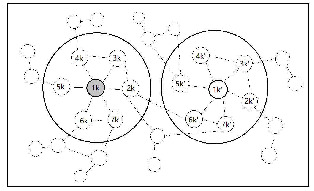
Figure 1: Egocentric network-based design. The figure represents two egocentric networks denoted by $k$ and $k^{\prime}$. Index participants are denoted as $1k$ and $1k^{\prime}$, and their network members are denoted as $ik$ and $ik^{\prime}$, with $i>1$. The treated index participant is represented by a grey solid circle. Solid circles represent in-sample units, while dashed circles represent out-of-sample units. Solid lines are the observed network connections between index participants and their network members, while dashed lines represent network connections that are not observed.

2.2 Non-overlapping egonetworks

We denote by $\mathcal{N}_{ik}$ the network neighborhood of unit $i$ in egonetwork $k$. In an ENR design, in the sample $\mathcal{N}$ we only observe information on connections of index participants, i.e., $\mathcal{N}_{1k}$, whereas connections of network members $ik$, with $i=2,\ldots,n_{k}$ are in general not observed. In an undirected network, the only connection that we observe for network members is the one with their index participants. However, in addition to possible unobserved connections with out-of-sample individuals, in principle network members $ik$ can be linked to other index participants $1k^{\prime}$, with $k^{\prime}\neq k$. Furthermore, connections among network members in the same egonetwork are not observed. Although by network transitivity it is likely that the peers of an index participant are also connected to each other, a fully connected egonetwork is not guaranteed and some pairs of network members of the same egonetwork may not be linked.

We make here a simplifying assumption that will be needed for the identification of causal effects. We assume that network members are only connected to one index participant in the sample and that index participants are not connected among themselves. Formally, we denote by $\mathcal{N}^{*}_{ik}\subset\mathcal{N}^{*}$ the network neighborhood of unit $i$ in egonetwork $k$ only including in-sample units. Then, we make the following assumption.

Assumption 1 (Non-overlapping Egonetworks).

$\mathcal{N}^{*}_{ik}\subset\mathcal{N}^{*}_{k}\quad\forall ik\in\mathcal{N}^{*}$

The plausibility of this assumption in HPTN 037 has already been discussed in Buchanan et al. (2018). The non-overlapping egonetworks assumption can be guaranteed by design by selecting index participants whose egocentric networks are unlikely to overlap.

We let $G_{ik}$ be the number of treated network neighbors for unit $i$ in egonetwork $k$. As already mentioned, network members may be connected with other individuals not in the sample. However, because we assume that individuals that are not in the sample cannot receive the treatment, $G_{ik}$ is given by the number of treated network neighbors in the sample, i.e., $G_{ik}=\sum_{\ell k\in\mathcal{N}^{*}_{ik}}Z_{\ell k}$. Furthermore, thanks to the non-overlapping network assumption (Assumption 1 and that in the egocentric network-based design network members cannot be treated), we have that the number of treated network neighbors is equal to the number of treated individuals in the same egonetwork, excluding the individual itself, i.e., $G_{ik}=\sum_{\ell k\in\mathcal{N}^{*}_{k},\ell\neq i}Z_{\ell k}=(1-R_{ik})Z_{1k}$. As a consequence, under the ENR design and under Assumption 1, index participants $1k$ have $Z_{1k}=\{0,1\}$ and $G_{1k}=0$, because they can be treated but cannot have any treated network neighbor, while network members $ik$, with $i>1$, have $Z_{ik}=0$ and $G_{ik}=Z_{1k}=\{0,1\}$, with the value of $G_{ik}$ depending on whether they are in an intervention or control network.

3 Interference and Causal Estimands

3.1 Neighborhood Interference

Under the potential outcome framework, we denote by $Y_{ik}(\mathbf{Z})$ the potential outcome of individual $i$ in network $k$ under the sample treatment vector $\mathbf{Z}$. Here, we relax the no-interference assumption, allowing for the outcome of an individual $i$ in egonetwork $k$ to be affected by their own treatment $Z_{ik}$ and also by the number of treated network neighbors $G_{ik}$. In the causal inference literature, this assumption is known as ‘neighborhood interference’, which restricts interference to the network neighborhood. In addition, we are assuming a unit’s potential outcome depends on a specific function of the neighbors’ treatment (Aronow and Samii, 2017; Ogburn et al., 2017; Forastiere et al., 2020). Formally:

Assumption 2 (Neighborhood Interference).

Given $\mathbf{Z}$ and $\mathbf{Z}^{\prime}$ such that $Z_{ik}=Z^{\prime}_{ik}$ and $G_{ik}=G^{\prime}_{ik}$, then $Y_{ik}(\mathbf{Z})=Y_{ik}(\mathbf{Z}^{\prime})$.

Under this assumption, we can index potential outcomes only by $Z_{ik}$ and $G_{ik}$: $Y_{ik}(z,g)$ denotes the potential outcome of participant $i$ in network $k$ under individual treatment $Z_{ik}=z$ and number of treated neighbors $G_{ik}=g$. Assumption 2 rules out the possibility that individuals’ behaviors are indirectly affected by the intervention received by other individuals with whom they are not directly connected (e.g., friends of friends). This assumption is satisfied if behavioral influence takes time to travel through the network and the time when the behavioral outcome is measured in the study only allows for influence to occur between network neighbors. In egonetwork studies, Assumption 2 is also plausible if egonetworks are sufficiently distant in the network, such that even if interference could occur beyond the network neighbors, the effect of the treatment received by one index participant would not reach individuals in other egonetworks. In HPTN 037 the plausibility of the neighborhood assumption is supported by both egonetwork distances and the outcome measure.

3.2 Causal Estimands

We define the average (individual) treatment effect (AIE) as the average effect of receiving the treatment when network neighbors are all untreated, that is:

$$\tau=\mathbb{E}\left[Y_{ik}(1,0)-Y_{ik}(0,0)\right].$$ (1)

Note that the expectation is taken over the distribution of potential outcomes in the population $\mathcal{M}$, under the common superpopulation perspective to causal inference (Hernán and Robins 2020). Similarly, we define the average spillover effect (ASpE) as the average effect of having one treated network neighbor versus none while the individual is untreated:

$$\delta=\mathbb{E}\left[Y_{ik}(0,1)-Y_{ik}(0,0)\right].$$ (2)

We are also interested in the overall effect, defined as the effect of being in an egonetwork where one unit is treated (intervention egonetwork) versus being in an egonetwork where no one is treated (control egonetwork). We can write the causal estimand as the average difference between the potential outcomes of the treated untreated units in an intervention network and the potential outcomes of the untreated units in the control networks:

$$\begin{array}[]{ll}O=\mathbb{E}\left[\sum_{z=0}^{1}\sum_{g=0}^{1}Y_{ik}(z,g)Pr(Z_{ik}=z,G_{ik}=g|Z_{1k}=1)\right]\\ \quad\quad-\mathbb{E}\left[\sum_{z=0}^{1}\sum_{g=0}^{1}(Y_{ik}(z,g)Pr(Z_{ik}=z,G_{ik}=g|Z_{1k}=0)\right]\\ \quad=\tau Pr(R_{ik}=1)+\delta Pr(R_{ik}=0),\end{array}$$ (3)

The proof of Equation (3) is given in the Appendix 7.3.3. When the egonetwork size is constant, i.e., $n_{k}=n\quad\forall k$, the overall effect is equal to $O=\frac{1}{n+1}(\tau+n\,\delta)$.

3.3 Identifying Assumption and Identification of Causal Effects

Given the characteristics of an egocentric network-based design, under Assumptions 1 and 2, and under additional assumptions detailed in the Appendix 7.2, including unconfoundedness, consistency, and random sampling, we can identify the causal effects of interest. In particular, we can identify AIE and ASpE from the observed data as $\tau=\mathbb{E}[Y_{ik}|Z_{ik}=1]-\mathbb{E}[Y_{ik}|Z_{ik}=0,G_{ik}=0]$ and $\delta=\mathbb{E}[Y_{ik}|G_{ik}=1]-\mathbb{E}[Y_{ik}|Z_{ik}=0,G_{ik}=0]$. Similarly, the overall effect can be identified from the observed data as $O=\mathbb{E}[Y_{ik}|Z_{ik}=1]Pr(R_{ik}=1)+\mathbb{E}[Y_{ik}|G_{ik}=1]Pr(R_{ik}=0)-\mathbb{E}[Y_{ik}|Z_{ik}=0,G_{ik}=0].$ The proofs of the identification are given in the Appendix 7.3.

4 Regression-based Estimators and Sample Size Calculation

In this section, we propose regression-based estimators for AIE, ASpE, and $O$. We also derive formulas for the required number of index participants for detecting each causal effect or causal effects with pre-specified power and Type I error rate. To do so, we assume that all index participants have the same number of network members, i.e., $n_{k}=n$ for $k=1,...,K$. This assumption can be achieved by design by limiting the number of network members that each index participant can nominate. If $n$ is sufficiently small, it is plausible that index participant would nominate at least $n$ network members. If the list of network members is censored, we can assume that censoring is non-informative given that the treatment is randomized to index participants.

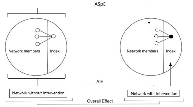
Figure 2: Egonetwork-based design and subsets of data used for the identification of each effect.

4.1 Statistical Models for the Average Treatment, Spillover, and Overall Effects

We introduce the regression model for estimating the average individual and spillover effects, $\tau$ and $\delta$, based on the identification results in Section 3.3. Under the stated assumptions, the AIE can be identified by comparing the outcomes of index participants in the intervention egonetworks (with $Z_{ik}=1$) to the outcomes of all individuals in the control egonetworks (with $Z_{ik}=0$ and $G_{ik}=0$), while the ASpE can be estimated by comparing the outcomes of networks members in the intervention egonetworks (with $G_{ik}=1$) to the outcomes of all individuals in the control egonetworks (with $Z_{ik}=0$ and $G_{ik}=0$) (Figure 6). Furthermore, we can identify the overall effect by comparing the outcomes of both the index participants and their network members in the intervention egonetworks to the outcomes of both the index participants and their network members in the control egonetworks. Alternatively, once $\tau$ and $\delta$ have been estimated, the overall effect can be estimated by $\widehat{O}=\frac{1}{(n+1)}(\widehat{\tau}+n\widehat{\delta})$.

For $k=1,...,K$ and $i=1,...,n+1$, we let

$$Y_{ik}=\gamma+\tau Z_{ik}+\delta G_{ik}+u_{k}+\epsilon_{ik},$$ (4)

where we assume that the residual error $\epsilon_{ik}\sim N(0,\sigma^{2}_{e})$ and the random egonetwork effect $u_{k}\sim N(0,\sigma^{2}_{u})$. In Model 4, the coefficient $\gamma$ is the mean outcome of individuals in networks without intervention, i.e., $\gamma=\mathbb{E}(Y_{ik}|Z_{ik}=0,G_{ik}=0)$. The coefficient $\tau$ is equal to $\mathbb{E}[Y_{ik}|Z_{ik}=1,G_{ik}=0]-\mathbb{E}[Y_{ik}|Z_{ik}=0,G_{ik}=0]$, which, under the previously stated assumptions, identifies the causal effect $\tau$ in Equation (1), i.e., the AIE. Finally, the coefficient $\delta$ is equal to $\mathbb{E}[Y_{ik}|Z_{ik}=0,G_{ik}=1]-\mathbb{E}[Y_{ik}|Z_{ik}=0,G_{ik}=0]$, which, in turn, under the previously stated assumptions, identifies the ASpE denoted as $\delta$ and defined in Equation (2).

To proceed, we let $\boldsymbol{\theta}=(\gamma,\tau,\delta)^{\prime}$ and further define $\mathbf{Y}_{k}=(Y_{1k},...,Y_{ik},...,Y_{(n+1)k})^{\prime}$ and $\mathbf{D}_{k}=(1,\mathbf{Z}_{k},\mathbf{G}_{k})$, where $\mathbf{Z}_{k}=(Z_{1k},...,Z_{(n+1)k})^{\prime}$ and $\mathbf{G}_{k}=(G_{1k},...,G_{(n+1)k})^{\prime}$. By design, $\mathbf{D}_{k}$ takes the specific forms: when $Z_{1k}=1$, $G_{1k}=0$ and $G_{ik}=1$ for $i>1$; when $Z_{1k}=0$, $Z_{ik}$ and $G_{ik}$ are always 0. By the sampling mechanism, as well as in Model 4, which in fact, models the distribution of the observed outcomes given the sampling mechanism and randomization, the observed outcomes of two individuals in different egonetworks are independent. The covariance between the observed outcomes of two members in the same egonetwork is $\text{Cov}(Y_{ik},Y_{i^{\prime}k}|\mathbf{Z}_{k},\mathbf{G}_{k})=\sigma^{2}_{u}$ for $i\neq i^{\prime}$ given $\mathbf{Z}_{k}$ and $\mathbf{G}_{k}$. Finally, the total variance of $Y_{ik}$, denoted by $\sigma^{2}_{Y}$, is equal to $\sigma^{2}_{u}+\sigma^{2}_{e}$. Then, the intra-class correlation (ICC) between $Y_{ik}$ and $Y_{i^{\prime}k}$, for $i\neq i^{\prime}$, conditional on $\mathbf{Z}_{k}$ and $\mathbf{G}_{k}$ is $\rho_{Y}=\frac{\sigma^{2}_{u}}{\sigma^{2}_{u}+\sigma^{2}_{e}}.$ As a result, the variance of the outcome vector $\mathbf{Y}_{k}$ for the $k$th egonetwork is $\text{Var}(\mathbf{Y}_{k}|\mathbf{Z}_{k},\mathbf{G}_{k})=\sigma^{2}_{Y}\cdot V_{k}$ with $V_{k}=(1-\rho_{Y})I_{(n+1)}+\rho_{Y}J_{(n+1)}$, where $I_{(n+1)}$ is a $(n+1)\times(n+1)$ identity matrix, $J_{(n+1)}$ is a $(n+1)\times(n+1)$ matrix where all elements are 1. Under this variance-covariance structure, we can estimate the parameter vector $\boldsymbol{\theta}$ of Model (4) using generalized least squares (GLS) as $\hat{\boldsymbol{\theta}}=\left(\sum\limits^{K}_{k=1}\mathbf{D}^{{}^{\prime}}_{k}V^{-1}_{k}\mathbf{D}_{k}\right)^{-1}\left(\sum\limits^{K}_{k=1}\mathbf{D}^{{}^{\prime}}_{k}\mathbf{Y}_{k}\right)$ with $\text{Var}(\hat{\boldsymbol{\theta}})=\sigma^{2}_{Y}\mathbf{U}^{-1}_{Ik},$ where $\mathbf{U}_{Ik}=\sum\limits^{K}_{k=1}\mathbf{D}^{{}^{\prime}}_{k}V^{-1}_{k}\mathbf{D}_{k}$. Under regularity conditions, as $K\to\infty$ and $n$ is fixed, $\sqrt{K}(\hat{\boldsymbol{\theta}}-\boldsymbol{\theta})$ is asymptotically normally distributed as $N(0,\Sigma_{I})$, where $\Sigma_{I}=\lim_{K\to\infty}\sigma^{2}_{Y}(\mathbf{U}_{Ik}/K)^{-1}=\sigma^{2}_{Y}\mathbf{U}_{I}^{-1}$ with $\mathbf{U}_{I}=\lim_{K\to\infty}\frac{1}{K}\mathbf{U}_{Ik}$.

We now use $\Sigma_{I}$ to construct the formulas for finding the required number of index participants for detecting different causal effects. In Appendix 7.4, we show that

$$\mathbf{U}_{I}=\left[\begin{array}[]{c|cc}\{c+(n+1)d\}(n+1)&\{c+(n+1)d\}p&\{c+(n+1)d\}np\\ \hline\cr\{c+(n+1)d\}p&(c+d)p&npd\\ \{c+(n+1)d\}np&npd&(c+nd)np\\ \end{array}\right]$$

with $c=\frac{1}{1-\rho_{Y}}$ and $d=-\frac{\rho_{Y}}{(1-\rho_{Y})(1+n\rho_{Y})}$. Then, the resulting lower-right block of $\Sigma_{I}$ is the covariance corresponding to $\tau$ and $\delta$, denoted as $\Sigma_{\tau\delta}$

$$\Sigma_{\tau\delta}=\sigma^{2}_{Y}\begin{bmatrix}\frac{cm_{2}+nd\sigma^{2}_{Z}}{cp\sigma^{2}_{Z}\{c+d(1+n)\}}&\frac{c(p-m_{1})-d\sigma^{2}_{Z}}{cp\sigma^{2}_{Z}\{c+d(1+n)\}}\\ \frac{c(p-m_{1})-d\sigma^{2}_{Z}}{cp\sigma^{2}_{Z}\{c+d(1+n)\}}&\frac{cm_{1}+d\sigma^{2}_{Z}}{ncp\sigma^{2}_{Z}\{c+d(1+n)\}}\\ \end{bmatrix},$$

where $\sigma^{2}_{Z}=p(1-p)$, $m_{1}=p(1-\frac{p}{n+1})$ and $m_{2}=p(1-\frac{np}{n+1})$. The derivation of $\Sigma_{\tau\delta}$ can be found in the Appendix 7.5.

4.2 Calculation of the Minimum Number of Networks

Based on Model (4) and the GLS estimator, we consider procedures for testing several hypotheses of potential interest related to the AIE, ASpE, and $O$. We then derive the required number of index participants to ensure adequate power to test the hypotheses of interest, given prespecified Type I error rate, significance level, and effect sizes. In the Appendix 7.8, we further provide formulas for the required number of network members given a specified number of index participants, a hypothesized effect size, a desired power and Type I error, as well as the minimum detectable effect size (MDE) given a specified number of index participants and network members, a desired power and Type I error.

The AIE hypothesis test (HIE). Here we test the hypothesis of no AIE; that is, $H_{0}:\tau=0$, against the alternative hypothesis $H_{1}:\tau\neq 0$. To test this hypothesis, we use the two-sided Z-test statistic: $T_{\tau}=\sqrt{K}(\hat{\tau}/\hat{\sigma}_{\tau})$, where $\sigma^{2}_{\tau}$ is the asymptotic variance of $\hat{\tau}$ from $\Sigma_{\tau\delta}$ (the top-left element in $\Sigma_{\tau\delta}$), $\sigma^{2}_{\tau}=\frac{\sigma^{2}_{Y}\{n(1-p)(1-\rho_{Y})+(1+n\rho_{Y})\}}{(n+1)\sigma^{2}_{Z}}$.

Given the GLS estimator for $\boldsymbol{\theta}$ in Model (4), $T_{\tau}$ asymptotically follows a standard normal distribution under the null hypothesis. Assume that the effect size of $\tau$ is $\Delta_{\tau}$. Given a Type I error rate $\alpha$, the probability of rejecting $H_{0}$ when it is true is $P(|T_{\tau}|>z_{1-\alpha/2}|\tau=0)$ with critical value $z_{1-\alpha/2}$. Then, the power of the test, $\pi_{\tau}=P\{|\sqrt{K}(\hat{\tau}-\Delta_{\tau})/\hat{\sigma}_{\tau})|\geq z_{1-\alpha/2}-\sqrt{K}\Delta_{\tau}/\sigma_{\tau}|\tau=\Delta_{\tau}\}=1-\Phi(z_{1-\alpha/2}-\sqrt{K}\Delta_{\tau}/\sigma_{\tau})+\Phi(z_{\alpha/2}-\sqrt{K}\Delta_{\tau}/\sigma_{\tau})$, where $\Phi(\cdot)$ is the cumulative distribution function of the standard normal distribution and $z_{\pi}=\Phi^{-1}(\pi)$ for any power $\pi\in[0,1]$. When the sample size of the two-sided test is calculated, the minuscule region associated with one of the tails based on whether the effect is positive or negative is often ignored. Thus, given the required power and Type I error rate $\alpha$, we solve $\pi_{\tau}$ ignoring the minuscule region for $K$ to obtain the required number of index participants for a specified effect size $\Delta_{\tau}$ for the HIE, that is,

$$\begin{array}[]{cl}K_{{\tau}}&=\frac{\sigma^{2}_{\tau}(z_{1-\alpha/2}+z_{\pi})^{2}}{\Delta_{\tau}^{2}}=\frac{\sigma^{2}_{Y}[n\{p(\rho_{Y}-1)+1\}+1](z_{1-\alpha/2}+z_{\pi})^{2}}{(n+1)\sigma^{2}_{Z}\Delta_{\tau}^{2}}.\end{array}$$ (5)

The ASpE hypothesis test (HSpE). Here, we focus on the hypothesis of no ASpE, $H_{0}:\delta=0$, against the alternative hypothesis $H_{A}:\delta\neq 0$. To test this hypothesis, we use the two-sized Z-test statistic: $T_{\delta}=\sqrt{K}(\hat{\delta}/\hat{\sigma}_{\delta})$, where $\sigma^{2}_{\delta}=\frac{\sigma^{2}_{Y}\{(1-p)(1-\rho_{Y})+n(1+n\rho_{Y})\}}{n(n+1)\sigma^{2}_{Z}},$ is the bottom-right element of $\Sigma_{\tau\delta}$ corresponding to $\hat{\delta}$.

Similar to above, $T_{\delta}$ follows a standard normal distribution under $H_{0}$. For a specified effect size $\Delta_{\delta}$ for the ASpE, a given Type I error rate $\alpha$, the power of the test is $\pi_{\delta}=1-\Phi(z_{1-\alpha/2}-\sqrt{K}\Delta_{\delta}/\sigma_{\delta})+\Phi(z_{\alpha/2}-\sqrt{K}\Delta_{\delta}/\sigma_{\delta})$. We can solve this equation for $K$ to obtain the required number of networks to achieve adequate power for the given Type I error rate, $\alpha$, and ignoring the minuscule region, by,

$$K_{{\delta}}=\frac{\sigma^{2}_{\delta}(z_{1-\alpha/2}+z_{\pi})^{2}}{\Delta_{\delta}^{2}}=\frac{\sigma^{2}_{Y}\{(1-p)(1-\rho_{Y})+n(1+n\rho_{Y})\}(z_{1-\alpha/2}+z_{\pi})^{2}}{n(1+n)\sigma^{2}_{Z}\Delta_{\delta}^{2}}.$$ (6)

The AIE and ASpE joint hypothesis test (HISpJ). When we are interested in testing both individual and spillover effects simultaneously, as would usually be the case in an egocentric network-based randomized design, we can construct a two degree of freedom Wald test for the joint hypothesis $H_{0}:\boldsymbol{\theta}_{J}=0$, where $\boldsymbol{\theta}_{J}=(\tau,\delta)^{\prime}$. The Wald test statistic of HISpJ is $Q_{J}=K\hat{\boldsymbol{\theta}}^{\prime}_{J}\hat{\Sigma}_{\delta\tau}^{-1}\hat{\boldsymbol{\theta}}_{J}$. From what has previously been shown about the asymptotic distribution of $\hat{\boldsymbol{\theta}}$, it follows that $\hat{\boldsymbol{\theta}}_{J}$ has a multivariate normal distribution asymptotically, with mean $\boldsymbol{\theta}_{J}$ and covariance $\Sigma_{\tau\delta}$. Then, $Q_{J}$ is asymptotical approximately $\chi^{2}$ distributed. Given a Type I error $\alpha$ and effect size $\Delta_{J}$, the power of this test is $\pi_{J}=P\{Q_{J}\geq\chi^{2}_{1-\alpha}(2)|\boldsymbol{\theta}_{J}=\Delta_{J}\}$. Then, the required number of index participants for HISpJ to have power $\pi_{J}$ at Type I error rate $\alpha$ can be obtained by solving $\pi_{J}\geq\pi$ for $K$. In the Appendix 7.6, we show that the required number of index participants is $K\geq\frac{\upsilon(\chi^{2}_{1-\alpha}(2),\pi,2)}{\Delta_{J}^{\prime}\Sigma_{\delta\tau}^{-1}\Delta_{J}},$ where $\upsilon(q,\pi,p_{T})$ is the non-centrality parameter of the non-central $\chi^{2}$ distribution with two degree of freedom whose $1-\pi$ quantile is equal to $q$. Then, the resulting required number of index participants for HISpJ is

$$K_{J}=\frac{\upsilon(\chi^{2}_{1-\alpha}(2),\pi,2)\sigma^{2}_{Y}(1+n\rho_{Y})}{\sigma^{2}_{Z}(\Delta_{\tau}^{2}+n\Delta_{\delta}^{2})}.$$ (7)

The AIE and ASpE conjunctive hypothesis test (HISpC). The HISpJ rejects the null hypothesis when at least one of AIE and ASpE has an effect on the outcome. However, sometimes we are interested in the case that the intervention is effective in terms of both the AIE and ASpE; that is, both causal effects are non-zero. A conjunctive hypothesis test can be used for this purpose with $H_{0}:\tau=0$ or $\delta=0$ against the alternative hypothesis $H_{A}:\tau\neq 0$ and $\delta\neq 0$ (Tian et al., 2022). To test this hypothesis, we use a bivariate test statistic $Q_{C}=(T_{\tau},T_{\delta})^{T}$, where $T_{\tau}$ and $T_{\delta}$ correspond to the HIE and HSpE, respectively. Then $Q_{C}$ follows a bivariate normal distribution $Q_{C}\overset{d}{\to}N\left(\begin{bmatrix}\sqrt{K}\Delta_{\tau}/\sigma_{\tau}\\ \sqrt{K}\Delta_{\delta}/\sigma_{\delta}\end{bmatrix},\Omega=\begin{bmatrix}1&\frac{\sigma_{\tau\delta}}{\sigma_{\tau}\sigma_{\delta}}\\ \frac{\sigma_{\tau\delta}}{\sigma_{\tau}\sigma_{\delta}}&1\end{bmatrix}\right),$ where $\sigma_{\tau\delta}=KCov(\hat{\tau},\hat{\delta})$ with $Cov(\hat{\tau},\hat{\delta})=\frac{\sigma^{2}_{Y}\{p(1+n\rho_{Y})+(1-p)(n+1)\rho_{Y}\}}{(n+1)\sigma^{2}_{Z}}.$ Then the power formula for the two-sided conjunctive test is

$$\begin{aligned} \pi_{C}&=\Pr[\{|T_{\tau}|>Z_{1-\alpha/2}\}\cap\{|T_{\delta}|>Z_{1-\alpha/2}\}]\\ &=\int^{\infty}_{Z_{1-\alpha/2}}\int^{\infty}_{Z_{1-\alpha/2}}u(T_{\tau},T_{\delta})dT_{\tau}dT_{\delta}+\int^{\infty}_{Z_{1-\alpha/2}}\int^{Z_{\alpha/2}}_{-\infty}u(T_{\tau},T_{\delta})dT_{\tau}dT_{\delta}\\ &+\int^{Z_{\alpha/2}}_{-\infty}\int^{\infty}_{Z_{1-\alpha/2}}u(T_{\tau},T_{\delta})dT_{\tau}dT_{\delta}+\int^{Z_{\alpha/2}}_{-\infty}\int^{Z_{\alpha/2}}_{-\infty}u(T_{\tau},T_{\delta})dT_{\tau}dT_{\delta}\end{aligned},$$ (8)

where $u(T_{\tau},T_{\delta})$ is the PDF of the bivariate normal distribution of $Q_{C}$ as discussed above. To find the required member of networks ($K_{C}$), we solve (8). This power formula can be used to numerically calculate the required number of networks because there is no closed form of this formula. A series of increasing integers $K$ can be plugged into the equation to compute the power after specifying the values of $\rho_{Y}$, $n$, $p$, $\Delta_{\tau}$, and $\Delta_{\delta}$.

The overall effect hypothesis test (HOE). When we are interested in testing the overall effect, we can construct a two-sided Z-test: $H_{0}:(\tau+n\delta)/(n+1)=0$. To test this hypothesis, we use the Z-test statistic: $T_{o}=\sqrt{K}\{(\hat{\tau}+n\hat{\delta})/(n+1)\}/\hat{\sigma}_{o}$, where $\sigma^{2}_{o}=\frac{\sigma^{2}_{Y}(1+n\rho_{Y})}{(n+1)\sigma^{2}_{Z}}$. $T_{o}$ is a linear transformation of $\hat{\tau}$ and $\hat{\delta}$, and follows a standard normal distribution when the effect size of the overall effect, $\Delta_{o}=(\Delta_{\tau}+n\Delta_{\delta})/(n+1)$ is zero. Similar to HIE and HSpE, given a Type I error $\alpha$, the power of the test is $\pi_{o}=1-\Phi(z_{1-\alpha/2}-\sqrt{K}\Delta_{o}/\sigma_{o})$. To find the required member of networks ($K_{o}$) at power $\pi_{o}$, we obtain

$$K_{o}=\frac{\sigma^{2}_{o}(z_{1-\alpha/2}+z_{\pi})^{2}}{\Delta_{o}^{2}}=\frac{\sigma^{2}_{Y}(1+n\rho_{Y})(z_{1-\alpha/2}+z_{\pi})^{2}}{(n+1)\sigma^{2}_{Z}\Delta_{o}^{2}}.$$ (9)

4.3 Investigation of the Sample Size for Each Hypothesis Test as a Function of Features of the Egocentric Network-based Design

To learn more about how $K$ changes with the other parameters, we investigate these relationships through some simulations. From (5) and (6), we observe that $K_{{\tau}}$ and $K_{{\delta}}$ are functions of $p$, the network size $n$, the intra-class correlation $\rho_{Y}$, and the effect sizes $\Delta_{\tau}$ and $\Delta_{\delta}$. In particular, we can see that the required number of networks, $K_{\tau}$ and $K_{\delta}$, increase with $\rho_{Y}$ and decrease with $n$. Smaller effect sizes $\Delta_{\tau}$ and $\Delta_{\delta}$ also inflate the required sample sizes of index participants for testing the AIE and the ASpE with sufficient power, respectively. From (7) and (9) we observe that $K_{J}$ and $K_{o}$ depend on $n$, $\rho_{Y}$, $p$ and the effect sizes of both $\tau$ and $\delta$. Smaller $\Delta_{\tau}$ and $\Delta_{\delta}$ inflate both $K_{J}$ and $K_{o}$. However, values $\Delta_{\tau}$ and $\Delta_{\delta}$ in different directions could result in a decrease or increase of $K_{J}$ and $K_{o}$. In practice with public health interventions, spillover effects are usually in the same direction as individual treatment effects. Moreover, as $K_{\tau}$ and $K_{\delta}$, the required number of networks $K_{J}$ and $K_{o}$ grow with $\rho_{Y}$ and decrease with network size $n$. The proofs of these claims are provided in the Appendix 7.7. We can also calculate the optimal $p$ to minimize the number of the networks, which satisfies the required power, depending on $n$ and $\rho_{Y}$ for testing AIE and ASpE, the formulas for calculating the optimal $p$ are given in Appendices 7.7.1 and 7.7.2.In Appendices 7.7.3 and 7.7.4, we demonstrate that $p=0.5$ is the optimal value for testing the overall effect, and also testing the AIE and the ASpE effect simultaneously for any $\rho_{Y}$ and $n$. We will evaluate the association between $K_{C}$ and the design parameters using numerical simulations because there is no closed form for $K_{C}$.

We further investigate the role of $\rho_{Y}$, the number of network members $n$ and the effect sizes $\Delta_{\tau}$ and $\Delta_{\delta}$ in testing the AIE, the ASpE, the overall effect, and multiple effects for the joint test and the conjunctive test using Model (4) with numerical simulations. For fixed $\sigma^{2}_{Y}$, $\Delta_{\tau}$ and $\Delta_{\delta}$ set to 1, we let the outcome ICC, $\rho_{Y}$, vary from (0 to 1), $n\in\{1,2,5,10\}$, and $p=c(0.3,0.5,0.7,0.9)$. Figure 3 shows the required number of networks for the four hypothesis tests, HIE, HSpE, HISpJ, HISpC, and HOE with $\alpha=5\%$ and $\pi=80\%$. To note, there is no solution for HISpC in some parameter combinations (e.g., $p=0.3,n=1$ case), thus the lines in Figure 3 are incomplete. For each $p$, the patterns of $K_{\tau}$, $K_{\delta}$, $K_{J}$, $K_{C}$, and $K_{o}$ with $\rho_{Y}$ and $n$ are displayed. Figure 4 highlights how the required number of index participants for the different tests varies with $p$ and $\rho_{Y}$ given $n=5$.

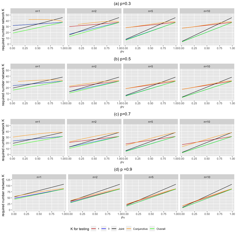
Figure 3: Comparison of the required number of networks for HIE, HSpE, HISpJ, HISpC, and HOE given different values of $p$, $n$, and $\Delta_{\tau}=\Delta_{\delta}$=1, $\sigma^{2}_{Y}=1$. Note that with $n=1$ the blue and red lines overlap meaning that $K_{\tau}=K_{\delta}$.

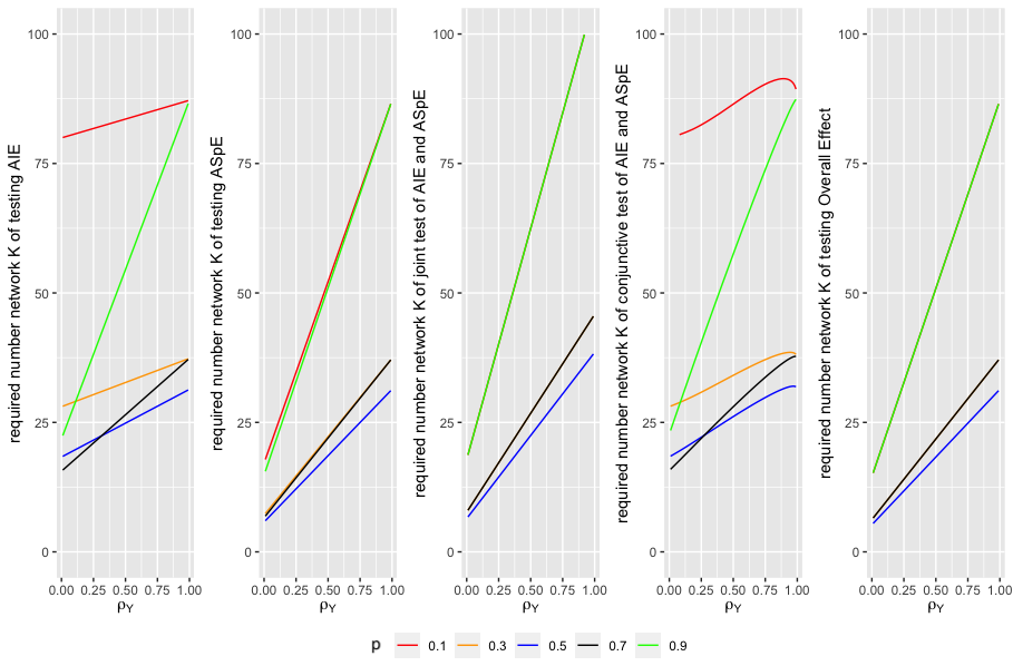
Figure 4: Required number of index participants for HIE, HSpE, HISpJ, HISpC, and HOE given different values of $p$: $\Delta_{\tau}=\Delta_{\delta}$=1, $\sigma^{2}_{Y}=1$, $n=5$. The lines with two colors mean the two lines overlap with each other.

4.4 Comparison of power and sample size for the hypotheses tests

To further compare the required sample sizes to detect different effects, we fixed $p=0.5$, as it is a common choice, and compute the ratios between the required number of index participants for the different hypotheses. The ratio between $K_{\delta}$ and $K_{\tau}$ is

$$K_{\delta/\tau}=\frac{K_{{\delta}}}{K_{{\tau}}}=\frac{(1-p)(1-\rho_{Y})+n(1+n\rho_{Y})}{n^{2}(1-p)(1-\rho_{Y})+n(1+n\rho_{Y})}\times r_{\tau/\delta}^{2},$$ (10)

where $r_{\tau/\delta}=\Delta_{\tau}/\Delta_{\delta}$ is the ratio between the AIE and the ASpE. As the individual effect becomes larger relative to the spillover effect, the number of index participants needed to assess the spillover effect becomes larger than the number needed to assess the individual effect. When $r_{\tau/\delta}=1$, it is straightforward to see that $K_{\delta/\tau}\leq 1$, which means that detecting the spillover effect equal in magnitude to the individual effect requires fewer egonetworks than needed to detect the AIE. Intuitively, this is because the estimation of spillover effects relies on the comparison between $nKp$ network members versus $(n+1)K(1-p)$ untreated network members and index participants, whereas the estimation of the AIE relies on the comparison between $Kp$ treated index participants versus $(n+1)K(1-p)$ untreated individuals. That is, the ASpE has $n$ more participants available for estimation than the AIE. Thus, when $r_{\tau/\delta}=1$ and $n=1$, then $K_{\tau}=K_{\delta}$. Let $\rho_{Y}=0$, we have $K_{\delta/\tau}=\frac{(1-p)+n}{n^{2}(1-p)+n}$, This means that the ratio decreases as $n$ increases, as can be seen in (10). When $n$ is large, we need many more index participants to obtain an adequately powered study for HIE than for HSpE. To investigate the relationship between $K_{\delta/\tau}$ and $\rho_{Y}$, we rewrite (10) as $K_{\delta/\tau}=\frac{\{n^{2}-(1-p)\}\rho_{Y}+n+1-p}{n^{2}p\rho_{Y}+n^{2}(1-p)+n}\times r_{\tau/\delta}$. For any fixed $n>1$ and $r_{\tau/\delta}$, $K_{\delta/\tau}$ decreases as $\rho_{Y}$ increases, which means $K_{\delta}$ and $K_{\tau}$ will get closer. In practice, $\rho_{Y}$ is usually not that large, for example, $\rho_{Y}\approx 0.115$ in HPTN 037.

To compare $K_{J}$ with $K_{\tau}$ and $K_{\delta}$, we investigate the ratios:

$$K_{J/\tau}=\frac{K_{J}}{K_{\tau}}=\frac{\upsilon(\chi^{2}_{1-\alpha}(2),\pi,2)}{(z_{1-\alpha/2}+z_{\pi})^{2}}\times\frac{(1+n\rho_{Y})(n+1)}{n(1-p)(1-\rho_{Y})+(1+n\rho_{Y})}\times r_{\tau/J}$$ (11)

and

$$K_{J/\delta}=\frac{K_{J}}{K_{\delta}}=\frac{\upsilon(\chi^{2}_{1-\alpha}(2),\pi,2)}{(z_{1-\alpha/2}+z_{\pi})^{2}}\times\frac{(1+n\rho_{Y})(n+1)n}{(1-p)(1-\rho_{Y})+n(1+n\rho_{Y})}\times r_{\delta/J},$$ (12)

where $r_{\tau/J}=\frac{\Delta^{2}_{\tau}}{\Delta^{2}_{\tau}+n\Delta^{2}_{\delta}}$ and $r_{\delta/J}=\frac{\Delta^{2}_{\delta}}{\Delta^{2}_{\tau}+n\Delta^{2}_{\delta}}$. It is clear that increasing $r_{\tau/J}$ inflates $K_{J/\tau}$. Since a larger $r_{\tau/J}$ indicates a larger $r_{\tau/\delta}$, we have that $K_{J/\tau}$ increases as the effect size ratio between $\tau$ and $\delta$ increases. We also observe that $r_{\delta/J}$ inflates $K_{J/\tau}$. Since $r_{\delta/J}$ increases as $r_{\tau/\delta}$ decreases, this confirms that $K_{J/\delta}$ increases as the effect size ratio between $\tau$ and $\delta$ decreases, that is, as the effect of spillover becomes larger relative to the individual treatment effect. When $\Delta_{\tau}=\Delta_{\delta}$, then (11) simplifies to $K_{J/\tau}=\frac{\upsilon(\chi^{2}_{1-\alpha}(2),\pi,2)}{(z_{1-\alpha/2}+z_{\pi})^{2}}\times\frac{(1+n\rho_{Y})}{n(1-p)(1-\rho_{Y})+(1+n\rho_{Y})}$ with $\upsilon(\chi^{2}_{1-\alpha}(2),\pi,2)/(z_{1-\alpha/2}+z_{\pi})^{2}\approx 1.227$ for $\alpha=0.05$. When $\rho_{Y}=0$, we then have $K_{J/\tau}=1.227/\{n(1-p)+1\}.$ We observe that for any $n$, $K_{J}<K_{\tau}$, which means that detecting the AIE requires more index participants than detecting the AIE and the ASpE simultaneously, and the ratio decreases as $n$ increases. This indicates that HIE is more sensitive to $n$ than HISpJ. With fixed $n$, as $\rho_{Y}$ increases, $r_{J/\tau}$ increases. This indicates that $K_{J}$ is more sensitive to $\rho_{Y}$ then $K_{\tau}$.

Similar to $K_{J/\tau}$, when $\Delta_{\tau}=\Delta_{\delta}$, we write (12) as $K_{J/\delta}=1.227\times\frac{n(1+n\rho_{Y})}{(1-p)(1-\rho_{Y})+n(1+n\rho_{Y})}.$ When $n>2$, $K_{J/\delta}$ is larger than 1. This means that we need more egonetworks to detect the AIE and the ASpE simultaneously than to detect the ASpE only when the index participant has more than two network members. When $n=1$ or 2, as $\rho_{Y}$ becomes larger, $K_{J}$ is first smaller than $K_{\delta}$, and then larger than $K_{\delta}$. Furthermore, given $n$, it is clear that an increase in $\rho_{Y}$ inflates $K_{J/\delta}$, as it dose with $K_{\tau}$, $K_{\delta}$ and $K_{J}$. This indicates that the increasing rate of $K_{J}$ as a function of $\rho_{Y}$ is greater than that of $K_{\delta}$. When $\rho_{Y}=0$, $K_{J/\delta}=1.227\times\frac{n}{n-p+1},$ which means $K_{J/\delta}$ increases as $n$ increases. It means that HISpJ depends more on $n$ than HSpE.

Last but not least, we compare $K_{\tau}$, $K_{\delta}$, and $K_{J}$ with $K_{o}$. We investigate the following ratios:

$$K_{\tau/o}=\frac{K_{\tau}}{K_{o}}=\frac{n(1-p)(1-\rho_{Y})+(1+n\rho_{Y})}{(n+1)^{2}(1+n\rho_{Y})}\times\left(1+\frac{2n}{r_{\tau/\delta}}+\frac{n^{2}}{r^{2}_{\tau/\delta}}\right),$$ (13)

$$K_{\delta/o}=\frac{K_{\delta}}{K_{o}}=\frac{(1-p)(1-\rho_{Y})+n(1+n\rho_{Y})}{n(n+1)(1+n\rho_{Y})}\times\left(r^{2}_{\tau/\delta}+2nr_{\tau/\delta}+n^{2}\right)$$ (14)

and

$$K_{J/o}=\frac{K_{J}}{K_{o}}=\frac{\upsilon(\chi^{2}_{1-\alpha}(2),\pi,2)}{(n+1)(z_{1-\alpha/2}+z_{\pi})^{2}}\times\frac{r^{2}_{\tau/\delta}+2nr_{\tau/\delta}+n^{2}}{r^{2}_{\tau/\delta}+n}.$$ (15)

From (13)-(15), we see that $K_{\tau/o}$ could either be larger or smaller than 1 depending on the magnitude of other parameters. We also observe that $K_{\tau/o}$ decreases as $p$, $\rho_{Y}$, or $r_{\tau/\delta}$ increasing. But $K_{\delta/o}$ is always larger than 1, which means that we need more egonetworks to test ASpE than OE given other parameters fixed. Similar to $K_{\tau/o}$, $K_{\delta/o}$ decreases as $p$ and $\rho_{Y}$ increases, but increasing $r_{\tau/\delta}$ inflates $K_{\delta/o}$. For $K_{J/o}$, when $n>r_{\tau/\delta}$, $K_{J/o}$ increases as $n$ increases; when $n<r$, $K_{J/o}$ decreases as $n$ increases. When $r_{\tau/\delta}<1$, $K_{J/o}$ increases as $r_{\tau/\delta}$ increases; when $r_{\tau/\delta}>1$, $K_{J/o}$ decreases as $r_{\tau/\delta}$ increases.

5 Illustrative Example: HPTN 037 Study

We use the HPTN 037 study to inform the design parameters and show how to estimate the required number of index participants given pre-specified power and level of significance for different hypothesis tests. The HPTN 037 study is an ENR experiment to assess the efficacy of a network-oriented peer education intervention to promote HIV risk reduction among injection drug users and their drug network members in Chiang Mai, Thailand, and Philadelphia, US. Here, we only include participants in the Philadelphia site (Latkin et al., 2009). At the baseline visit, eligible index participants were those who injected drugs at least 12 times in the prior three months, and eligible network members were those who injected drugs with the relevant index participant within the prior three months. Index participants received network-oriented peer educator training sessions during a four-week period and two booster sessions at six and 12 months of study participation.

The primary outcome considered here is the average number of drug injection risk behaviors in the month prior to each visit, averaged across the number of visits each individual attended up to the 30-month visit. Here, we consider “using rinse water that others had used” as the risk injection behavior to illustrate our approach. To make the estimation result more robust, we removed the index participants and the network members whose average number of risk injection behaviors lie more than 1.5 times the interquartile range. The remaining 186 networks have a number of network members ranging between 1 and 6, with an average of 2 (sd=1.15). The intervention assignment probability, $p$, was 0.47, with 88 intervention egonetworks and 98 control egonetworks. The outcome variance and the outcome ICC were $\sigma_{Y}^{2}=1.02$ and $\rho_{Y}\approx 0.115$, with an outcome mean of 0.53. The ASpE and the the AIE were estimated to be $-0.34$ (95% CI:$[-0.61,-0.08]$) and $-0.32$ (95% CI:$[-0.63,-0.01]$), respectively. This means that the average number of drug injection risk behaviors of the treated index participants is 0.32 less than that of the untreated index participants, and the average number of drug injection risk behaviors of the network members whose index participants were treated is 0.34 less than that of the network members whose index participants were not treated. We approximately follow these features of HPTN 037 to set the design parameters. Table 1 shows the required number of egonetworks needed for HIE, HSpE, HISpJ, HISpC, and HOE, to ensure 80% power to detect the effects, with number of network members equal to 2, with different effect sizes, $p$, and $\rho_{Y}$. We varied these design parameters approximately around the values estimated in HPTN 037 to assess the sensitivity of $K$ to these changes. In particular, we set the the effect size of both the AIE and the ASpE to 0.5 times, 1 times, and 1.5 times the value of -0.35, approximately the value estimated in HPTN 037. We also varied $p$ and $\rho_{Y}$ using the values $[0.5,0.3,0.7]$ and $[0.1,0.2,0.05]$, respectively. Using equations (5)-(9) to calculate $K_{\tau}$, $K_{\delta}$, $K_{J}$, $K_{C}$ and $K_{o}$, we found that when $\rho_{Y}=0.10$ and $p=0.50$, $K_{\delta}=122$ and $K_{\tau}=251$ egonetworks are required to ensure $80\%$ power to detect the ASpE and AIE with sizes similar to that observed in HPTN 037, i.e., $\Delta_{\delta}=-0.35$ and $\Delta_{\tau}=-0.35$. To detect either the AIE or the ASpE, the AIE and the ASpE simultaneously and the overall effect with $80\%$ power, we need $K_{J}=126$, $K_{C}=195$ and $K_{o}=103$, respectively. When we shifted the design parameters, we observed similar patterns as shown in Figure 3. In summary, given the parameters estimated from HPTN 037, the HOE requires the smallest number of networks, and the HISpJ requires the largest number of networks. Increasing assignment probability $p$ or decreasing outcome ICC requires less index participants for all the hypothesis tests. Amplifying the effect sizes reduces the required number of index participants to detect the causal effects.

Table 1: Required number of networks for Hypothesis Test 1-4 with $n=2$, and $\sigma^{2}_{Y}=1.02$
in HPTN 037

Parameter		$\Delta_{\delta}=-0.350$						$\Delta_{\delta}=-0.175$						$\Delta_{\delta}=-0.525$
		$K_{\delta}$	$K_{\tau}$	$K_{J}$	$K_{C}$	$K_{o}$		$K_{\delta}$	$K_{\tau}$	$K_{J}$	$K_{C}$	$K_{o}$		$K_{\delta}$	$K_{\tau}$	$K_{J}$	$K_{C}$	$K_{o}$
$\rho_{Y}$	$p$	Case 1: $\Delta_{\tau}=-0.350$						Case 1: $\Delta_{\tau}=-0.350$						Case 1: $\Delta_{\tau}=-0.350$
0.1	0.5	122	180	126	195	103		487	180	252	489	231		55	180	69	180	58
	0.3	155	251	153	268	123		617	251	300	622	275		69	251	82	251	69
	0.7	136	177	150	195	123		544	177	300	544	275		61	177	82	178	69
0.2	0.5	137	188	147	206	120		547	188	294	548	270		61	188	81	189	68
	0.3	171	257	175	278	143		684	257	350	686	321		76	257	96	257	81
	0.7	155	192	175	211	143		619	192	350	619	321		69	192	96	192	81
0.05	0.5	115	176	116	189	94		458	176	231	460	212		51	176	63	176	53
	0.3	146	248	138	263	112		583	248	275	591	252		65	248	75	248	63
	0.7	127	170	138	186	112		506	170	275	506	252		57	170	75	170	63
		Case 2: $\Delta_{\tau}=-0.525$						Case 2: $\Delta_{\tau}=-0.525$						Case 2: $\Delta_{\tau}=-0.525$
0.1	0.5	122	80	89	131	76		487	80	138	487	148		55	80	56	87	46
	0.3	155	112	106	173	90		617	112	164	617	176		69	112	67	120	55
	0.7	136	79	106	140	90		544	79	164	543	176		61	79	67	87	55
0.2	0.5	137	84	104	144	88		547	84	161	547	173		61	84	66	92	54
	0.3	171	114	124	185	105		684	114	191	684	206		76	114	78	124	64
	0.7	155	85	124	158	105		619	85	191	618	206		69	85	78	94	64
0.05	0.5	115	78	82	125	70		458	78	126	458	136		51	78	52	84	42
	0.3	146	110	97	167	83		583	110	150	583	162		65	110	62	117	50
	0.7	127	76	97	132	83		506	76	150	506	162		57	76	62	83	50
		Case 3: $\Delta_{\tau}=-0.70$						Case 3: $\Delta_{\tau}=-0.70$						Case 3: $\Delta_{\tau}=-0.70$
0.1	0.5	122	45	63	123	58		487	45	84	487	103		55	45	45	63	37
	0.3	155	63	75	156	69		617	63	100	617	123		69	63	53	85	44
	0.7	136	45	75	136	69		544	45	100	543	123		61	45	53	66	44
0.2	0.5	137	47	74	137	68		547	47	98	547	120		61	47	52	68	44
	0.3	171	65	88	172	81		684	65	117	683	143		76	65	62	89	52
	0.7	155	48	88	155	81		619	48	117	618	143		69	48	62	73	52
0.05	0.5	115	44	58	115	53		458	44	77	457	94		51	44	41	61	34
	0.3	146	62	69	148	63		583	63	92	583	112		65	62	49	82	41
	0.7	127	43	69	127	63		506	43	92	505	112		57	43	49	62	41

6 Conclusion and Discussion

The no-interference assumption is naturally violated by participants with social or physical interactions in a network. Few studies have been able to estimate the ASpE with sufficient power. The lack of methods for designing studies to detect the ASpE motivates us to propose an egonetwork-based design in which only a single index participant in treated networks receives the intervention. In this ENR design, we can estimate the AIE, the ASpE, and the overall effect simultaneously with a regression model. We developed closed-form sample size formulas for calculating the required number of index participants to power the hypothesis tests of detecting several causal estimands of interest. We investigated the patterns of how the required number of index participants changes with design parameters. In addition, we considered an alternative model to estimate and test the AIE and the ASpE using two separate linear mixed effect models in the Appendix 7.9. Comparing to the model proposed in Section 4, the alternative model allows the outcomes of index participants and their network members to have different total variances, but it requires greater index participants for testing the AIE and ASpE.

This work is affected by a few limitations. The study design assumes the same number of members in each network. Our methods could be further extended to handle variable network sizes, as in Manatunga et al. (2001). In HPTN 037, for example, the mean network size was 2, but it varies from 1 to 6, thus including the variation of the network size would possibly change the required number of networks. Furthermore, we used asymptotic statistical results to construct the sample size formulas, and their accuracy in finite samples could be further studied. We could also consider index and/or individual covariates that may lead to heterogeneity of the spillover effect. Design of studies to assess heterogeneity in the ASpE, AIE, and AOE will be considered in future work. To facilitate the use of our proposed design, we will also develop software for sample size calculation and power analysis.

7 Appendix

7.1 Population Notation and Egocentric Notation

7.1.1 Population Notation

Let us denote by $\mathcal{M}$ a population of interest and by $\mathcal{G}$ an undirected network being the graphical representation of this population, which consists of the pair $(\mathcal{M},E)$, where $\mathcal{M}$ is the set of units (or nodes) and $E$ is the set of edges representing the links between two units in $\mathcal{M}$. In Section 2.1, we have denoted individuals by $ik$, where $k$ is the egonetwork indicator. However, in a ENT design, individuals are sampled from a population $\mathcal{M}$ using an egocentric strategy, where we first sample index participants and then information is collected on their network members. Therefore, egonetworks are entities that are generated after sampling. In fact, in the population $\mathcal{M}$ each individual have their own egocentric networks (or network neighborhood), regardless of whether they are going to be sampled as an index participant, a network member, or not sampled at all. In addition, egocentric networks of individuals overlap, given that multiple individuals can share the same network neighbor (e.g., friend or sex partner). For this reason, the egonetwork notation $ik$ cannot be used in the population, for which we must use a single index notation $m$, such that $\mathcal{M}=\{m\}_{1}^{M}$. In a ENT design, we can also denote by $\mathcal{R}\subset\mathcal{M}$ the set of index participants.

Using the population notation, the set of edges $E$ in the graph $\mathcal{G}$ can be represented by $E=\{e_{mq}\}_{m,q\in\mathcal{M}}$, where each edge $e_{mq}$ represents a link between two units $m$ and $q$. We now denote by $\mathcal{N}_{m}=\{q\in\mathcal{M}:e_{mq}\in E\}$ the set of units sharing a link with unit $m$, i.e., the ‘network neighbors’ of unit $m\in\mathcal{R}$. Then, the study sample $\mathcal{N}\subset\mathcal{M}$ consists of all the index participants and their social network members, i.e., $\mathcal{N}=(\mathcal{R},\bigcup_{m\in\mathcal{R}}\mathcal{N}_{m})$.

In Section 2.1, we define the variables of interest, including the treatment, using the egonetwork notation. Using the population notation we can denote by $Z_{m}$ the treatment of unit $m\in\mathcal{M}$. The assumption that all units that are not in the sample are considered as not treated because they cannot receive the intervention implies that $Z_{m}=0,\forall m\notin\mathcal{N}$. We can also denote by $G_{m}$ the number of treated network neighbors of unit $m$, i.e., $G_{m}=\sum_{q\in\mathcal{N}_{m}}Z_{m}$. However, because we assume that individuals that are not in the sample cannot receive the treatment, $G_{m}=\sum_{q\in\mathcal{N}_{m}\cap\,\mathcal{N}}Z_{m}$.

7.1.2 Relation between the Population Notation and Egocentric Notation

In Section 2.1, for the sake of simplicity, we relabel the units in the sample $\mathcal{N}$ with the notation commonly used with clustered data. We let $k=1,...,K$ be the egonetwork indicator in $\mathcal{N}$. We then let $ik$ be the unit $i$ in egonetwork $k$, with $i=1,\ldots,n_{k}+1$. In particular, we let $1k$ represent the $k$th index participant and $ik$, with $i=2,...,n_{k}+1$, represents a network member of the egonetwork $k$. We refer to this notation as the egonetwork notation.

The relation between the population notation and the egonetwork notation can be explained by mapping functions. The egonetwork indicator $k$ is such that $m=r(k)\in\mathcal{R}$, with $r(\cdot)$ being some function mapping the $k$-th index participant to a unit in the population $\mathcal{R}$. Hence, $\mathcal{N}_{r(k)}$ represents the set of network members of the $k$-th index participant of size $n_{k}=|\mathcal{N}_{r(k)}|$. Similarly, $q=n(ik)\in\mathcal{N}_{r(k)}$ is the population indicator for $i$-th network member in the egonetwork $k$, with $n(\cdot)$ being some function mapping the $i$-th network member of the $k$-th index participant to a unit in the population $\mathcal{M}$. In general, we have that $m=h(ik)\in\mathcal{N}$ is the population indicator corresponding to the sample unit $ik$, where $h(1k)=r(k)$ and $h(ik)=n(ik)$ for $i=1,\dots,n_{k}$.

7.1.3 Non-overlapping Egonetworks Assumptions

In Section 2.2, we have introduced the non-overlapping egonetworks assumption (Assumption 1) under this egonetwork notation. Using the population indexing, we can formalize the non-overlapping egonetworks assumption in an alternative way. We denote by $\mathcal{C}_{k}=r(k)\cup\mathcal{N}_{r(k)}$ the set of units in the egonetwork $k$, including both the index participant and the network members. The non-overlapping assumption can be formalized by assuming that $\bigcap_{k=1}^{K}\mathcal{C}_{k}=\emptyset$. This assumption implies that $\mathcal{N}_{h(ik)}\bigcap\mathcal{C}_{k^{\prime}}=\emptyset$, that is, the network neighborhood of a unit $h(ik)\in\mathcal{N}$ may include units that are not in the sample but cannot include those that are in other egonetworks. The non-overlapping egonetworks assumption can be guaranteed by design by selecting index participants whose egocentric networks are unlikely to overlap. For example, we could use a block (or stratified) design. In particular, we would divide the sample into clusters (e.g., disparate geographical areas) such that units of different clusters are not connected, and sample only one index participant per cluster.

7.1.4 Neighborhood Interference and Stratified Interference

It is worth mentioning the relationship between the neighborhood interference assumption (Assumption 2) and the common stratified interference assumption Hudgens and Halloran (2008). The latter rules interference between groups allowing interference only between groups (partial interference) and assumes that interference depends only on the number of treated individuals in the same group and not on who they are (Hudgens and Halloran, 2008; Buchanan et al., 2018). Under the specific egocentric network-based design, where only index participants can be treated, and under the non-overlapping egonetworks assumption, the neighborhood interference assumption (Assumption 2) is equivalent to the stratified interference assumption with groups being the egonetworks. In fact, as already shown, $G_{ik}$, which is by definition equal to the number of network neighbors, i.e., $G_{ik}=\sum_{\ell k\in\mathcal{N}^{*}_{ik}}Z_{\ell k}$, in this setting will also be equal to the number of the other individuals in the same egonetwork who are treated, i.e., $G_{ik}=\sum_{\ell k\in\mathcal{N}^{*}_{k},\ell\neq i}Z_{\ell k}$. In the egocentric network-based study, $Z_{ik}$ and $G_{ik}$ can only take value 0 or 1 since at most one participant can be treated in an egonetwork.

7.2 Identifying Assumptions

Under the randomization scheme of the ENR design, the following unconfoundedness assumption holds:

Assumption 3 (Unconfoundedness of the treatment in the egocentric network-based design).

$Y_{ik}(z,g)\perp Z_{ik}|R_{ik}=1\text{ and }Y_{ik}(z,g)\perp G_{ik}|R_{ik}=0$

Assumption 3 states that for index participants the treatment is randomized (it doesn’t depend on the potential outcomes), and for network members the treatment of their indexes is randomized. Due to the randomization of the treatment to the index participants and under Assumption 1, given the participants’ index status, Assumption 3 is satisfied. Here, Assumption 1 ensures that $G_{ik}=0$ given $R_{ik}=1$, and $Z_{ik}=0$ given $R_{ik}=0$, thus, Assumption 3 can also be written as $Y_{ik}(z,g)\perp Z_{ik}|(R_{ik}=1,G_{ik})$ and $Y_{ik}(z,g)\perp G_{ik}|(R_{ik}=0,Z_{ik})$. Furthermore, we make here the assumption of random sampling.

Assumption 4 (Random Sampling).

$Y_{ik}(z,g)\perp R_{ik}$

This assumption states that potential outcomes do not depend on whether the unit is an index participant or a network member, that is, index participants are randomly sampled from the population and network members can also be seen as such. Assumption 4 could be problematic if index participants self-select themselves to serve in this role. In this case, index participants and network members may differ in terms of their characteristics. If this self-selection is a concern, one can estimate the individual effect only among index participants and the spillover effect only among network members. In this case, the comparison group for the estimation of the individual effect would only include untreated index participants, while the comparison group for the estimation of the spillover effect would only include network members of untreated index participants.

It can be shown that the unconfoundedness assumption (Assumption 3), specific to the egocentric network-based design, and the random sampling assumption (Assumption 4) guarantee the following unconfoundedness of the joint treatment. The proof of Assumption 5 is given in Appendix 7.2.1.

Assumption 5 (Unconfoundedness of the joint treatment).

$Y_{ik}(z,g)\perp Z_{ik},G_{ik}$

This assumption implies that both the individual treatment $Z_{ik}$ and the number of treated neighbors $G_{ik}$ are as good randomized. Under Assumptions 1, 3 and 4, then Assumption 5 is satisfied for $(z,g)=\{(0,0),(0,1),(1,0)\}$.

Finally, to relate observed outcomes to potential outcomes, we make the following assumption, known as ‘consistency’.

Assumption 6 (Consistency).

Denote by $Y_{ik},Z_{ik},G_{ik}$ the observed values of the outcome, the treatment, and the number of treated neighbors of unit $i$ in egonetwork $k$. Then, the following holds: $Y_{ik}=Y_{ik}(Z_{ik},G_{ik})$

7.2.1 Proof of Assumption 5

In this section, we show Assumption 5 is satisfied for $(Z_{ik},G_{ik})=\{(0,0),(0,1),(1,0)\}$. We fist give the general form of $P\{Z_{ik}=z,G_{ik}=g|Y_{ik}(z^{\prime},g^{\prime})\}$:

$$P\{Z_{ik}=z,G_{ik}=g|Y_{ik}(z^{\prime},g^{\prime})\} =\sum\limits^{1}_{r=0}P\{Z_{ik}=z,G_{ik}=g|Y_{ik}(z^{\prime},g^{\prime}),R_{ik}=r\}P(R_{ik}=r|Y_{ik}(z^{\prime},g^{\prime})\}$$

$$=\sum\limits^{1}_{r=0}P\{Z_{ik}=z,G_{ik}=g|Y_{ik}(z^{\prime},g^{\prime}),R_{ik}=r\}P(R_{ik}=r)$$

$$=P\{Z_{ik}=z|Y_{ik}(z^{\prime},g^{\prime}),G_{ik}=g,R_{ik}=1\}P(G_{ik}=g|R_{ik}=1)P(R_{ik}=1)$$

$$\quad+P\{G_{ik}=g|Y_{ik}(z^{\prime},g^{\prime}),Z_{ik}=z,R_{ik}=0\}P(Z_{ik}=z|R_{ik}=0)P(R_{ik}=0),$$

where the second step is due to Assumption 4. Then we show Assumption 5 case by case.

1. Case for $(Z_{ik},G_{ik})=(0,0)$:

$$P\{Z_{ik}=0,G_{ik}=0|Y_{ik}(z^{\prime},g^{\prime})\} =P\{Z_{ik}=z|Y_{ik}(z^{\prime},g^{\prime}),G_{ik}=0,R_{ik}=1\}P(R_{ik}=1)$$

$$+P\{G_{ik}=g|Y_{ik}(z^{\prime},g^{\prime}),Z_{ik}=0,R_{ik}=0\}P(R_{ik}=0)$$

$$=P(Z_{ik}=0|G_{ik}=0,R_{ik}=1)P(R_{ik}=1)$$

$$+P\{G_{ik}=0|Z_{ik}=0,R_{ik}=0\}P(R_{ik}=0)$$

$$=P(Z_{ik}=0,G_{ik}=0|R_{ik}=1)P(R_{ik}=1)$$

$$+P\{Z_{ik}=0,G_{ik}=0|R_{ik}=0\}P(R_{ik}=0)$$

$$=P(Z_{ik}=0,G_{ik}=0),$$

where the second step is due to Assumption 1 and Assumption 3.

2. Case for $(Z_{ik},G_{ik})=(1,0)$:

$$P\{Z_{ik}=1,G_{ik}=0|Y_{ik}(z^{\prime},g^{\prime})\} =P\{Z_{ik}=1|Y_{ik}(z^{\prime},g^{\prime}),G_{ik}=0,R_{ik}=1\}P(R_{ik}=1)$$

$$=P(Z_{ik}=1|G_{ik}=0,R_{ik}=1)P(R_{ik}=1)$$

$$=P(Z_{ik}=1,G_{ik}=0|R_{ik}=1)P(R_{ik}=1)$$

$$=P(Z_{ik}=1,G_{ik}=0|R_{ik}=1)P(R_{ik}=1)$$

$$+P(Z_{ik}=1,G_{ik}=0|R_{ik}=0)P(R_{ik}=0)$$

$$=P(Z_{ik}=1,G_{ik}=0),$$

where the first step is due to Assumption 1, Assumption 3 and $P(Z_{ik}=1|R_{ik}=0)=0$, the last step is due to $P(Z_{ik}=1,G_{ik}=0|R_{ik}=0)=0$.

3. Case for $(Z_{ik},G_{ik})=(0,1)$:

$$P\{Z_{ik}=0,G_{ik}=1|Y_{ik}(z^{\prime},g^{\prime})\} =P\{G_{ik}=1|Y_{ik}(z^{\prime},g^{\prime}),Z_{ik}=0,R_{ik}=0\}P(R_{ik}=0)$$

$$=P(G_{ik}=1|Z_{ik}=0,R_{ik}=0)P(R_{ik}=0)$$

$$=P(Z_{ik}=0,G_{ik}=1|R_{ik}=0)P(R_{ik}=0)$$

$$=P(Z_{ik}=0,G_{ik}=1),$$

where the first step is due to Assumption 1, Assumption 3, and $P(G_{ik}=1|R_{ik}=1)=0$, the last step isdue to $P(Z_{ik}=0,G_{ik}=G|R_{ik}=1)=0$.

Assumption 5 is satisfied by combing the results of Cases 1-3 above.

7.3 Non-parametric Identification

Given the characteristics of an egocentric network-based design, and under Assumptions 1, 2, 5, and 6, we can identify the causal estimands from the observed data. In the following subsections, we report the identification results for each estimand and their proof.

7.3.1 Non-parametric Identification of $\tau$

For the individual effect $\tau$, we have

$$\tau=\mathbb{E}\big{[}Y_{ik}(1,0)-Y_{ik}(0,0)\big{]}=\mathbb{E}\{Y_{ik}|Z_{ik}=1\}-\mathbb{E}\{Y_{ik}|Z_{ik}=0,G_{ik}=0\}.$$

Proof: We have

$$\mathbb{E}\big{[}Y_{ik}(1,0)\big{]} =\mathbb{E}\{Y_{ik}(1,0)|Z_{ik}=1,G_{ik}=0\}$$

$$=\mathbb{E}\{Y_{ik}|Z_{ik}=1,G_{ik}=0\}$$

$$=\mathbb{E}\{Y_{ik}|Z_{ik}=1\},$$

where the first step is due to the unconfoudedness assumption (Assumption 5), the second step is using the consistency property (Assumption 6), and the third step is due to the egocentric randomization. We also have

We also have

$$\mathbb{E}\big{[}Y_{ik}(0,0)\big{]} =\mathbb{E}\{Y_{ik}(0,0)|Z_{ik}=0,G_{ik}=0\}$$

$$=\mathbb{E}\{Y_{ik}|Z_{ik}=0,G_{ik}=0\},$$

where the first step is due to the unconfoudedness assumption (Assumption 5), and the second step is using the consistency property (Assumption 6). As a result,

$$\mathbb{E}\big{[}Y_{ik}(1,0)-Y_{ik}(0,0)\big{]}=\mathbb{E}\big{[}Y_{ik}(1,0)\big{]}-\mathbb{E}\big{[}Y_{ik}(0,0)\big{]}=\mathbb{E}\{Y_{ik}|Z_{ik}=1\}-\mathbb{E}\{Y_{ik}|Z_{ik}=0,G_{ik}=0\}.$$

7.3.2 Non-parametric Identification of $\delta$

For the spillover effect $\delta$, we have

$$\delta=\mathbb{E}\big{[}Y_{ik}(0,1)-Y_{ik}(0,0)\big{]}=\mathbb{E}[Y_{ik}|G_{ik}=1]-\mathbb{E}[Y_{ik}|Z_{ik}=0,G_{ik}=0].$$

Proof: Similar to the proof of identification for $\tau$, for $\delta$ we have

$$\mathbb{E}\big{[}Y_{ik}(0,1)\big{]} =\mathbb{E}\{Y_{ik}(0,1)|Z_{ik}=0,G_{ik}=1\}$$

$$=\mathbb{E}\{Y_{ik}|Z_{ik}=0,G_{ik}=1\}$$

$$=\mathbb{E}\{Y_{ik}|G_{ik}=1\},$$

and

$$\mathbb{E}\big{[}Y_{ik}(0,0)\big{]} =\mathbb{E}\{Y_{ik}(0,0)|Z_{ik}=0,G_{ik}=0\}$$

$$=\mathbb{E}\{Y_{ik}|Z_{ik}=0,G_{ik}=0\}.$$

As a result, $\delta=\mathbb{E}[Y_{ik}|G_{ik}=1]-\mathbb{E}[Y_{ik}|Z_{ik}=0,G_{ik}=0]$.

7.3.3 Non-parametric Identification of Overall effect $O$

For the overall effect $O$, we have

$$O =\mathbb{E}\left[\sum_{z=0}^{1}\sum_{g=0}^{1}Y_{ik}(z,g)Pr(Z_{ik}=z,G_{ik}=g|Z_{1k}=1)\right]$$

$$\quad-\mathbb{E}\left[\sum_{z=0}^{1}\sum_{g=0}^{1}(Y_{ik}(z,g)Pr(Z_{ik}=z,G_{ik}=g|Z_{1k}=0)\right]$$

$$=\mathbb{E}\left[\sum_{r=0}^{1}\sum_{z=0}^{1}\sum_{g=0}^{1}Y_{ik}(z,g)Pr(Z_{ik}=z,G_{ik}=g|Z_{1k}=1,R_{ik}=r)Pr(R_{ik}=r)\right]$$

$$\quad-\mathbb{E}\left[\sum_{r=0}^{1}\sum_{z=0}^{1}\sum_{g=0}^{1}(Y_{ik}(z,g)Pr(Z_{ik}=z,G_{ik}=g|Z_{1k}=1,R_{ik}=r)Pr(R_{ik}=r)\right]$$

$$=\mathbb{E}\left[Y_{ik}(1,0)Pr(R_{ik}=1)+Y_{ik}(0,1)Pr(R_{ik}=0)\right]-\mathbb{E}\left[\sum_{r=0}^{1}(Y_{ik}(0,0)Pr(R_{ik}=r)\right]$$

$$=\tau Pr(R_{ik}=1)+\delta Pr(R_{ik}=0),$$

where we have used that $Pr(Z_{ik}=1,G_{ik}=0|Z_{1k}=1,R_{ik}=1)=1$, $Pr(Z_{ik}=0,G_{ik}=1|Z_{1k}=1,R_{ik}=0)=1$, and $Pr(Z_{ik}=0,G_{ik}=0|Z_{1k}=0,R_{ik}=r)=1$. Then the identification of $O$ can be shown by plugging in the identification results of $\tau$ and $\delta$.

7.4 Variance for Regression Coefficients

We have $\Sigma_{I}=\lim_{K\to\infty}\sigma^{2}_{Y}(\mathbf{U}_{Ik}/K)^{-1}$ and $\mathbf{U}_{I}=\lim_{K\to\infty}\mathbf{U}_{Ik}/K$. Then $\mathbf{U}_{I}$ can be written as (Yang et al. 2020):

$$\mathbf{U}_{Ik}=cS_{Ik}+dT_{Ik}$$

with

$$S_{Ik}=\sum\limits^{K}_{k=1}\begin{bmatrix}n+1&Z_{1k}&nG_{2k}\\ Z_{1k}&Z^{2}_{1k}&0\\ nG_{2k}&0&nG^{2}_{2k}\end{bmatrix}$$

and

$$T_{Ik}=\sum\limits^{K}_{k=1}\begin{bmatrix}(n+1)^{2}&(n+1)Z_{1k}&n(n+1)G_{2k}\\ (n+1)Z_{1k}&Z^{2}_{1k}&nZ_{1k}G_{2k}\\ n(n+1)G_{2k}&nZ_{1k}G_{2k}&n^{2}G^{2}_{2k},\end{bmatrix}$$

where $c=\frac{1}{1-\rho_{Y}}$ and $d=-\frac{\rho_{Y}}{(1-\rho_{Y})(1+n\rho_{Y})}$. Then

$$S_{I}=\lim_{K\to\infty}\frac{1}{K}S_{Ik}=\begin{bmatrix}n+1&p&np\\ p&p&0\\ np&0&np\end{bmatrix}$$

and

$$T_{I}=\lim_{K\to\infty}\frac{1}{K}T_{Ik}=\begin{bmatrix}(n+1)^{2}&(n+1)p&n(n+1)p\\ (n+1)p&p&np\\ n(n+1)p&np&n^{2}p\end{bmatrix}.$$

As a result,

$$\mathbf{U}_{I}=cS_{I}+dT_{I}=\left[\begin{array}[]{c|cc}\{c+(n+1)d\}(n+1)&\{c+(n+1)d\}p&\{c+(n+1)d\}np\\ \hline\cr\{c+(n+1)d\}p&(c+d)p&npd\\ \{c+(n+1)d\}np&npd&(c+nd)np\\ \end{array}\right]$$

7.5 Derivation of $\Sigma_{\tau\delta}$

From Section 7.4, we have

$$\mathbf{U}_{I}=\left[\begin{array}[]{c|cc}\{c+(n+1)d\}(n+1)&\{c+(n+1)d\}p&\{c+(n+1)d\}np\\ \hline\cr\{c+(n+1)d\}p&(c+d)p&npd\\ \{c+(n+1)d\}np&npd&(c+nd)np\\ \end{array}\right]=\left[\begin{array}[]{c|c}A&B\\ \hline\cr C&D\\ \end{array}\right]$$

with $c=\frac{1}{1-\rho_{Y}}$ and $d=-\frac{\rho_{Y}}{(1-\rho_{Y})(1+n\rho_{Y})}$. We split $U_{I}$ into a $2\times 2$ blockwise matrix for further matrix inversion. $\Sigma_{\tau\delta}$, the lower-right element of $\Sigma_{I}$, which is $\lim_{K\to\infty}\sigma^{2}_{Y}(\mathbf{U}_{Ik}/K)^{-1}$, is the corresponding covariance for $\tau$ and $\delta$, is calculated by $\sigma^{2}_{Y}\times(D-CA^{-1}B)^{-1}$. Thus, $\Sigma_{\tau\delta}$ can be written as

$$\Sigma_{\tau\delta}=\frac{\sigma^{2}_{Y}}{E_{4}}\begin{bmatrix}A_{4}&B_{4}\\ C_{4}&D_{4}\\ \end{bmatrix},$$

$$A_{4}=(c+nd)np-\frac{n^{2}p^{2}}{n+1}\{c+(n+1)d\}=ncp\left\{1-\frac{np}{(n+1)}\right\}+n^{2}dp(1-p),$$

$$B_{4}=C_{4}=\frac{np^{2}}{n+1}\{c+(n+1)d\}-ndp=\frac{ncp^{2}}{n+1}-ndp(1-p),$$

$$D_{4}=(c+d)p-\frac{p^{2}}{n+1}\{c+(n+1)d\}=cp\left\{1-\frac{p}{(n+1)}\right\}+dp(1-p),$$

and

$$E_{4}=A_{4}\times D_{4}-B_{4}\times C_{4}$$

We let $\sigma^{2}_{Z}=p(1-p)$, $m_{1}=p(1-\frac{p}{n+1})$ and $m_{2}=p(1-\frac{np}{n+1})$. Then

$$A_{4}=ncm_{2}+n^{2}d\sigma_{Z}^{2},\quad B_{4}=C_{4}=nc(p-m_{1})-nd\sigma^{2}_{Z},\quad D_{4}=cm_{1}+d\sigma^{2}_{Z}$$

and

$$E_{4} =nc\{cp(m_{1}+m_{2}-p)+d\sigma^{2}_{Z}p(1+n)\}$$

$$=ncp\{cp(1-p)+d\sigma^{2}_{Z}(1+n)\}$$

$$=ncp\{c\sigma^{2}_{Z}+d\sigma^{2}_{Z}(1+n)\}$$

$$=ncp\sigma^{2}_{Z}\{c+d(1+n)\}.$$

Using the fact that $(p-m_{2})=n(p-m_{1})$, the formula of $\Sigma_{\tau\delta}$ can be simplified as

$$\Sigma_{\tau\delta}=\sigma^{2}_{Y}\begin{bmatrix}\frac{cm_{2}+nd\sigma^{2}_{Z}}{cp\sigma^{2}_{Z}\{c+d(1+n)\}}&\frac{c(p-m_{1})-d\sigma^{2}_{Z}}{cp\sigma^{2}_{Z}\{c+d(1+n)\}}\\ \frac{c(p-m_{1})-d\sigma^{2}_{Z}}{cp\sigma^{2}_{Z}\{c+d(1+n)\}}&\frac{cm_{1}+d\sigma^{2}_{Z}}{ncp\sigma^{2}_{Z}\{c+d(1+n)\}}\\ \end{bmatrix}.$$

7.6 The Minimum Number of Network Required for HISpJ

In this section, we provide the derivation of the minimum number of index participants required for HISpJ. Our derivation is based on a general jointly hypothesis test $H_{0}:L\boldsymbol{\theta}_{J}=0$, where $\boldsymbol{\theta}_{J}=(\tau,\delta)^{\prime}$ and $L$ is the matrix to construct the jointly hypothesis test. Then the Wald test statistic is given by

$$Q_{J}=K(L\hat{\boldsymbol{\theta}}_{J})^{\prime}(L\hat{\Sigma}^{-1}_{\tau\delta}L^{\prime})(L\hat{\boldsymbol{\theta}}_{J}).$$

We have known that from Generalized least squares, $\sqrt{K}(\hat{\boldsymbol{\theta}}_{J}-\boldsymbol{\theta}_{J})\xrightarrow{d}N(0,\Sigma_{\tau\delta})$ as $K\to\infty$. Then $\sqrt{K}(L\hat{\boldsymbol{\theta}}_{J}-L\boldsymbol{\theta}_{J})\xrightarrow{d}N(0,L\Sigma_{\tau\delta}L^{\prime})$ as $K\to\infty$. As a result, $L\hat{\boldsymbol{\theta}}_{J}$ can be presented as

$$L\hat{\boldsymbol{\theta}}_{J}=\frac{1}{\sqrt{K}}(L\Sigma_{\tau\delta}L^{\prime})^{\frac{1}{2}}W_{q}+L\boldsymbol{\theta}_{J},$$

where $W_{q}$ is a $q$-length vector following a standard multivariate normal distribution. Then we can write the test statistic, $Q_{J}$ as

$$Q_{J}=K\left\{\frac{1}{\sqrt{K}}(L\Sigma_{\tau\delta}L^{\prime})^{\frac{1}{2}}W_{q}+L\boldsymbol{\theta}_{J}\right\}^{\prime}(L\hat{\Sigma}^{-1}_{\tau\delta}L^{\prime})\left\{\frac{1}{\sqrt{K}}(L\Sigma_{\tau\delta}L^{\prime})^{\frac{1}{2}}W_{q}+L\boldsymbol{\theta}_{J}\right\}.$$

It has the same asymptotic distribution as

$$Q^{*}_{J} =\{(L\Sigma_{\tau\delta}L^{\prime})^{\frac{1}{2}}W_{q}+\sqrt{K}L\boldsymbol{\theta}_{J}\}^{\prime}(L\Sigma^{-1}_{I4}L^{\prime})\{(L\Sigma_{\tau\delta}L^{\prime})^{\frac{1}{2}}W_{q}+\sqrt{K}L\boldsymbol{\theta}_{J}\}$$

$$=\{W_{q}+\sqrt{K}(L\Sigma_{\tau\delta}L^{\prime})^{-\frac{1}{2}}L\boldsymbol{\theta}_{J}\}^{\prime}\{W_{q}+\sqrt{K}(L\Sigma_{\tau\delta}L^{\prime})^{-\frac{1}{2}}L\boldsymbol{\theta}_{J}\}$$

$$=\sum\limits^{q}_{l=1}(W_{q,l}+\sqrt{K}L_{\boldsymbol{\theta},l})^{2},$$

where $W_{q,l}$ is the $l$th element in $W_{q}$ and $L_{\boldsymbol{\theta},l}$ is the $l$th element of $L_{\boldsymbol{\theta}}=(L\Sigma_{\tau\delta}L^{\prime})^{-\frac{1}{2}}L\boldsymbol{\theta}_{J}$.

Then the minimum number of networks required for HISpJ to have power $\pi$ should satisfy

$$\Pr\{Q^{*}_{J}\geq\chi^{2}_{1-\alpha}(q)|L\boldsymbol{\theta}_{J}=L\Delta_{J}\}\geq\pi.$$ (16)

So it suffices to let

$$K\sum\limits^{q}_{l=1}L^{2}_{\boldsymbol{\theta},l}\geq\upsilon(\chi^{2}_{1-\alpha}(q),\pi,q)$$

to satisfy (16). Thus, we have that

$$K \geq\frac{\upsilon(\chi^{2}_{1-\alpha}(q),\pi,q)}{\sum\limits^{q}_{l=1}L^{2}_{\boldsymbol{\theta},l}}$$

$$=\frac{\upsilon(\chi^{2}_{1-\alpha}(q),\pi,q)}{(L\boldsymbol{\theta}_{J})(L\Sigma_{I4}L^{\prime})^{-1}(L\boldsymbol{\theta}_{J})^{\prime}}.$$

To be specific, for the hypothesis test of testing individual and spillover effects simultaneously, we use $\upsilon(\chi^{2}_{1-\alpha}(2),\pi,2)$ and $L$ is the $2\times 2$ diagonal matrix to find $K_{J}$.

7.7 The first derivative of $K$ with respect to $\rho_{Y}$, $p$, $n$, and effect size

In this section, We provide the first derivative of $K$ with respect to $\rho_{Y}$, $p$, $n$, and effect size, respectively, to investigate how the number of index participants changes with these design parameters.

7.7.1 The first derivative of $K_{\tau}$

We first provide the first derivative of $K_{\tau}$ in equation (5) with respect to $\rho_{Y}$:

$$\frac{\partial K_{\tau}}{\partial\rho_{Y}} =\frac{\sigma^{2}_{Y}n(z_{1-\alpha/2}+z_{\pi})^{2}}{\Delta_{\tau}^{2}\cdot(n+1)(1-p)}.$$ (17)

We can learn that (17) is always positive, so $K_{\tau}$ will monotonically increase as $\rho_{Y}$ increases.

The first derivative of $K_{\tau}$ with respect to $n$:

$$\frac{\partial K_{\tau}}{\partial n}=-\frac{\sigma^{2}_{Y}(z_{1-\alpha/2}+z_{\pi})^{2}\cdot\left(\rho_{Y}-1\right)}{\Delta_{\tau}^{2}\cdot\left(p-1\right)\left(n+1\right)^{2}}$$ (18)

We can observe that $K_{\tau}$ will monotonically decrease as $n$ increases since (18) is always negative.

The first derivative of $K_{\tau}$ with respect to $p$:

$$\frac{\partial K_{\tau}}{\partial p} =\frac{\sigma^{2}_{Y}(z_{1-\alpha/2}+z_{\pi})^{2}\cdot\left\{\left(\rho_{Y}-1\right)np^{2}+\left(2n+2\right)p-n-1\right\}}{\Delta_{\tau}^{2}\cdot\left(n+1\right)\left(p-1\right)^{2}p^{2}}$$ (19)

From (19), we cannot observe a monotone change of $K_{\tau}$ with $p$. However, given other parameters fixed, by letting $\frac{\partial K_{\tau}}{\partial p}=0$ and solve it for $p$, we could obtain the unique solution of $p\in[0,1]$:

$$\begin{aligned} p=\frac{(n+1)+\sqrt{(n+1)(1+n\rho_{Y})}}{(1-\rho_{Y})n}\end{aligned},$$

which minimize $K_{\tau}$.

The first derivative of $K_{\tau}$ with respect to $\Delta_{\tau}$ is

$$\frac{\partial K_{\tau}}{\partial\Delta_{\tau}} =\frac{2\sigma^{2}_{Y}(z_{1-\alpha/2}+z_{\pi})^{2}\cdot\left\{\left(\rho_{Y}-1\right)np+n+1\right\}}{\left(n+1\right)\left(p-1\right)p\Delta_{\tau}^{3}}$$ (20)

where we can observe that $K_{\tau}$ will monotonically decreases as $\Delta_{\tau}$ increases.

7.7.2 The first derivative of $K_{\delta}$

We first provide the first derivative of $K_{\delta}$ in (6) with respect to $\rho_{Y}$:

$$\frac{\partial K_{\delta}}{\partial\rho_{Y}} =\dfrac{\sigma^{2}_{Y}(z_{1-\alpha/2}+z_{\pi})^{2}\cdot\left(p+n^{2}-1\right)}{\Delta_{\delta}^{2}n\cdot\left(n+1\right)\left(1-p\right)p}$$ (21)

We can learn that (21) is always positive, so $K_{\delta}$ will monotonically increase as $\rho_{Y}$ increases.

The first derivative of $K_{\delta}$ with respect to $n$:

$$\frac{\partial K_{\delta}}{\partial n} =\frac{\sigma^{2}_{Y}(z_{1-\alpha/2}+z_{\pi})^{2}\cdot\left(\rho_{Y}-1\right)\cdot\left(n^{2}+\left(2-2p\right)n-p+1\right)}{\Delta_{\delta}^{2}\cdot\left(1-p\right)pn^{2}\cdot\left(n+1\right)^{2}}$$ (22)

We can learn that (22) is always negative, so $K_{\delta}$ will monotonically decrease as $n$ increases.

The first derivative of $K_{\delta}$ with respect to $p$:

$$\frac{\partial K_{\delta}}{\partial p} =\frac{\sigma^{2}_{Y}(z_{1-\alpha/2}+z_{\pi})^{2}\cdot\left\{\left(\rho_{Y}-1\right)p^{2}+\left(2\rho_{Y}n^{2}+2n-2\rho_{Y}+2\right)p-\rho_{Y}n^{2}-n+\rho_{Y}-1\right\}}{\Delta_{\delta}^{2}n\cdot\left(n+1\right)\left(p-1\right)^{2}p^{2}}$$ (23)

$$=\frac{\sigma^{2}_{Y}(z_{1-\alpha/2}+z_{\pi})^{2}\cdot\left[(\rho_{Y}-1)p^{2}+(2p-1)\{\rho_{Y}(n-1)+1\}(n+1)\right]}{\Delta_{\delta}^{2}n\cdot\left(n+1\right)\left(p-1\right)^{2}p^{2}}$$

From (23), we cannot observe a monotone change of $K_{\delta}$ with $p$. Given $p\in[0,1]$, there exist only one solution for $\frac{\partial K_{\delta}}{\partial p}=0$, which is

$$\begin{aligned} p=\frac{(n^{2}\rho_{Y}+n-\rho_{Y}+1)\left(1-\sqrt{\frac{n^{2}\rho_{Y}+n-\rho_{Y}+1}{n^{2}\rho_{Y}+n-2\rho_{Y}+2}}\right)}{1-\rho_{Y}}\end{aligned}.$$

The first derivative of $K_{\delta}$ with respect to $\Delta_{\delta}$ is

$$\frac{\partial K_{\delta}}{\partial\Delta_{\delta}} =\frac{2\sigma^{2}_{Y}(z_{1-\alpha/2}+z_{\pi})^{2}\cdot\left\{\left(\rho_{Y}-1\right)p+\rho_{Y}n^{2}+n-\rho_{Y}+1\right\}}{n\cdot\left(n+1\right)\left(p-1\right)p\Delta_{\delta}^{3}}$$ (24)

where we can observe that $K_{\delta}$ will monotonically decrease as $\Delta_{\delta}$ increases.

7.7.3 The first derivative of $K_{o}$

We first provide the first derivative of $K_{o}$ in equation (9) with respect to $\rho_{Y}$:

$$\frac{\partial K_{o}}{\partial\rho_{Y}} =\frac{\sigma^{2}_{Y}(z_{1-\alpha/2}+z_{\pi})^{2}n}{\Delta_{o}^{2}\left(n+1\right)\left(1-p\right)p}$$ (25)

We can learn that (25) is always positive, so $K_{o}$ will monotonically increase as $\rho_{Y}$ increases.

The first derivative of $K_{o}$ with respect to $n$:

$$\frac{\partial K_{o}}{\partial n} =\dfrac{\sigma^{2}_{Y}(z_{1-\alpha/2}+z_{\pi})^{2}\cdot\left[\left\{\left(\rho_{Y}+1\right)\Delta_{\delta}-2\rho_{Y}\Delta_{\tau}\right\}n+2\Delta_{\delta}+\left(-\rho_{Y}-1\right)\Delta_{\tau}\right]}{\left(p-1\right)p\cdot\left(\Delta_{\delta}+\Delta_{\tau}\right)^{3}}$$ (26)

We observe that the change of $K_{O}$ is related to the magnitude of the effect size of $\tau$ and $\delta$.

The first derivative of $K_{o}$ with respect to $p$:

$$\frac{\partial K_{o}}{\partial p} =\frac{\sigma^{2}_{Y}(z_{1-\alpha/2}+z_{\pi})^{2}\cdot\left(\rho_{Y}n+1\right)\cdot\left(2p-1\right)}{\Delta_{\delta}^{2}\cdot\left(n+1\right)\left(p-1\right)^{2}p^{2}}$$ (27)

From (27), we can observe that when $p=0.5$, $K_{O}$ will take the optimal value. Meanwhile, $K_{O}$ decreases first and then increases as $p$ increases from 0 to 1.

7.7.4 The first derivative of $K_{J}$

We first provide the first derivative of $K_{J}$ in equation (7) with respect to $\rho_{Y}$:

$$\frac{\partial K_{J}}{\partial\rho_{Y}} =\frac{\sigma^{2}_{Y}\upsilon(\chi^{2}_{1-\alpha}(2),\pi,2)n}{\left(\Delta_{\delta}^{2}n+\Delta_{\tau}^{2}\right)\left(1-p\right)p}$$ (28)

We can learn that (28) is always positive, so $K_{J}$ will monotonically increase as $\rho_{Y}$ increases.

We first provide the first derivative of $K_{J}$ with respect to $n$:

$$\frac{\partial K_{J}}{\partial n} =\frac{\sigma^{2}_{Y}\upsilon(\chi^{2}_{1-\alpha}(2),\pi,2)\cdot\left(\Delta_{\delta}^{2}-\rho_{Y}\Delta_{\tau}^{2}\right)}{\left(p-1\right)p\cdot\left(\Delta_{\delta}^{2}n+\Delta_{\tau}^{2}\right)^{2}}$$ (29)

We observe that the change of $K_{J}$ is related to the magnitude of the effect size of $\tau$ and $\delta$.

The first derivative of $K_{J}$ with respect to $p$:

$$\frac{\partial K_{J}}{\partial p} =\dfrac{\sigma^{2}_{Y}\upsilon(\chi^{2}_{1-\alpha}(2),\pi,2)\cdot\left(\rho_{Y}n+1\right)\cdot\left(2p-1\right)}{\left(\Delta_{\delta}^{2}n+\Delta_{\tau}^{2}\right)\left(p-1\right)^{2}p^{2}}$$ (30)

From (30), we can observe that when $p=0.5$, $K_{J}$ will take the optimal value. Meanwhile, $K_{J}$ decreases first and then increases as $p$ increases from 0 to 1.

7.8 Calculation of Network Size $n$ and the Minimum Detectable Effect Size (MDE)

In the study design, we are also interested in calculating the required number of network members given a specified number of index participants, a hypothesized effect size, a desired power and Type I error, as well as the minimum detectable effect size (MDE) given a specified number of index participants and network members, a desired power and Type I error.

Using (5), (6) and (9), the MDE of $\tau$, $\delta$ and $O$ are

$$\Delta_{\tau} =\sqrt{\frac{\sigma^{2}_{Y}[n\{p(\rho_{Y}-1)+1\}+1](z_{1-\alpha/2}+z_{\pi})^{2}}{(n+1)\sigma^{2}_{Z}K}},$$

$$\Delta_{\delta}=\sqrt{\frac{\sigma^{2}_{Y}\{(1-p)(1-\rho_{Y})+n(1+n\rho_{Y})\}(z_{1-\alpha/2}+z_{\pi})^{2}}{n(n+1)\sigma^{2}_{Z}K_{\delta}}},$$

and

$$\Delta_{o}=\sqrt{\frac{\sigma^{2}_{Y}(1+n\rho_{Y})(z_{1-\alpha/2}+z_{\pi})^{2}}{(n+1)\sigma^{2}_{Z}K_{o}}}.$$

The MDE of HISpJ incorporates $\Delta_{\tau}$ and $\Delta_{\delta}$ at the same time. Given the given $K$, $n$, $\rho_{Y}$, $\sigma^{2}_{Y}$, $p$ and fixed power and type I error rate, $\alpha$, we have the solution to the implicit equations

$$\Delta_{\tau}=\sqrt{\frac{\upsilon(\chi^{2}_{1-\alpha}(2),\pi,2)\sigma^{2}_{Y}(1+n\rho_{Y})}{K_{J}\sigma^{2}_{Z}}-n\Delta_{\delta}^{2}}.$$

and

$$\Delta_{\delta}=\sqrt{\frac{\upsilon(\chi^{2}_{1-\alpha}(2),\pi,2)\sigma^{2}_{Y}(1+n\rho_{Y})}{nK_{J}\sigma^{2}_{Z}}-\frac{\Delta_{\tau}}{n}}.$$

To obtain the minimum number of network members for each index participant, we solve the sample size equation (5), (6), (7) and (9) with respect to $n$, given pre-specified $K$ and other sample size parameters for each hypothesis test. Then, the problem now involves finding the root of non-linear equations, which some packages in the statistical software could solve. In this paper, we use multiroot in R to obtain the solutions. To be specific, here we use AIE as an example to show the calculation details of $n$. From Section 4.2, we know the sample size equation of testing AIE is (5). Then the equation needs to be solved is $K_{\tau}-K=0$, where $K$ is the pre-specified sample size given required power and Type I error, $\alpha$. In most of the cases, we could obtain one or multiple solutions, where the smallest one is selected as the optimal result. However, under some situations, there is no solution for $n$ for each index participant given the sample size equation, and other design parameters. This phenomenon has been seen in other clustered studies. To overcome this obstacle, one could consider modifying the pre-specified parameters. Usually, we could increase the number of index participants, $K_{\tau}$, by each unit, and then solve the equation again until the solution is founded. For HISpC, without the closed form of the sample size $K_{C}$, we used the power function (8) instead of the sample size equation to find $n$. We solve $\pi_{C}-\pi=0$, given a pre-specified power and other design parameters. Figure 5 shows an example that how $n$ changes with $\rho_{Y}$ for HIE, HSpE, HOE, HISpJ, and HISpC by solving (5), (6), (7) and (9) equal to 30 or (8) equals to 80%, given $p=0.5$, $\Delta_{\tau}=\Delta_{\delta}$, $\sigma^{2}_{Y}=1$. We could observe that for all five tests, $n$ increases as $\rho_{Y}$ increased. To note, for HISpJ, we cannot obtain a reasonable $n$ when $\rho_{Y}>0.77$. Under this situation, we could increase $K$ to overcome this problem, such as $n=0.85$ when $K=35$ and $\rho_{Y}=0.8$.

Solving the sample size equation or power function is not the only way to find $n$. One could treat this problem as an optimization problem by setting the power function as the objective function. Then, we could find the minimum $n$ maximizing the power with different parameter constraints, such as the test should at least achieve the required power, or the study has the maximum number of networks.

We aslo use HPTN 037 (Latkin et al. 2009) to demonstrate how to estimate MDE and $n$ given $K$, pre-specified power and Type I error for the hypothesis tests considered in this paper We inverted equations (5), (6) and (9) to obtain the absolute minimum detectable effect sizes for the AIE, ASpE, and overall effect to be $|0.34|$, $|0.28|$, an $|0.26|$, respectively, for different value of $\rho_{Y}$ and $p$ (Table 2), with pre-specified power $80\%$ and Type I error rate $5\%$. In Table 3, we also provide the minimum required network sizes $n$ for the HIE, HSpE, HISpJ, HISpC, and HOE. Given $\tau=-0.35$, we cannot obtain $n_{\tau}$ and $n_{C}$ to achieve the required 80% power and $\alpha=0.05$ for HIE when $p=0.30$. As we discussed in this section, we could increase $K$ to obtain an applicable $n$. For example, when we increase $K=250$, $n_{\tau}=2.02$, and $n_{C}=2.89$ for the case of $\rho_{Y}=0.10$ and $p=0.30$.

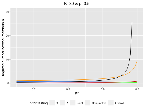
Figure 5: Required number of network members for HIE, HSpE, HISpJ, HISpC, and HOE given different values of $\rho_{Y}\in[0.1,0.8]$ to achieve 80% power: $\Delta_{\tau}=\Delta_{\delta}$=1, $\sigma^{2}_{Y}=1$, $p=0.5$, $K=30$.

Table 2: Minimum absolute values of detectable effect sizes given 186 networks, $n=2$, $\sigma^{2}_{Y}=1$, $\alpha=0.05$ and 80% power

Design Parameters		HIE	HSPE	HOE
$\rho_{Y}$	p	$|\Delta_{\tau}|$	$|\Delta_{\delta}|$	$|\Delta_{o}|$
0.10	0.50	0.34	0.28	0.26
	0.30	0.41	0.32	0.28
	0.70	0.34	0.30	0.28
0.20	0.50	0.35	0.30	0.28
	0.30	0.41	0.34	0.31
	0.70	0.36	0.32	0.31
0.05	0.50	0.40	0.28	0.25
	0.30	0.34	0.31	0.27
	0.70	0.34	0.29	0.27

Table 3: Minimum required network members given 186 index participants with $\tau=-0.35$,
$\delta=-0.35$, $\sigma^{2}_{Y}=1$, $\alpha=0.05$ and 80% power

Design Parameters		HIE	HSPE	HISpJ	HISpC	HOE
$\rho_{Y}$	p	$n_{\tau}$	$n_{\delta}$	$n_{J}$	$n_{C}$	$n_{o}$
0.10	0.50	1.62	1.1	0.84	2.40	0.45
	0.30	ND	1.57	1.28	ND	0.78
	0.70	1.67	1.22	1.28	2.30	0.78
0.20	0.50	2.28	1.18	1.06	3.29	0.53
	0.30	ND	1.75	1.72	ND	0.97
	0.70	2.37	1.39	1.72	3.23	0.97
0.05	0.50	1.41	1.07	0.77	2.14	0.41
	0.30	ND	1.50	1.14	ND	0.71
	0.70	1.45	1.15	1.14	2.03	0.71
In this example, ND represents for not discovered.

7.9 Alternative Regession-based Estimators

7.9.1 Statistical Model

We consider two separate regression models for estimating the AIE and the ASpE based on the identification results in Section 3.2. Implicitly, the AIE is estimated by comparing the outcomes of index participants in the networks with intervention with those in the networks without intervention, while the ASpE is estimated by comparing the outcomes between networks members in networks with/out intervention (Figure 6). For $i=1$, we have

$$Y_{1k}=\gamma_{\tau}+\tau Z_{1k}+\epsilon_{1k}$$ (31)

and for $i=2,...,(n+1)$,

$$Y_{ik}=\gamma_{\delta}+\delta G_{ik}+u_{k}+\epsilon_{ik},$$ (32)

where we assume $\epsilon_{1k}\sim N(0,\sigma^{2}_{e1})$, $\epsilon_{ik}\sim N(0,\sigma^{2}_{e})$, $u_{k}\sim N(0,\sigma^{2}_{u})$ and $\epsilon_{ik}\perp u_{k}$. We also assume $\sigma^{2}_{e}$ and $\sigma^{2}_{u}$ are known. We let $\theta_{I}=(\gamma_{\tau},\tau)^{\prime}$ and $\theta_{II}=(\gamma_{\delta},\delta)^{\prime}$.

In model (31), $\gamma_{\tau}$ is the mean of index participants in networks without intervention, which is estimated by $\mathbb{E}[Y_{1k}|Z_{1k}=0]$. The estimate of $\tau$ in model (31) is $\mathbb{E}[Y_{1k}|Z_{1k}=1]-\mathbb{E}[Y_{1k}|Z_{1k}=0]$, which is same as the identification of the AIE using the observed data in Section 3.2. In model (32), $\gamma_{\delta}$ is the mean of network members in the networks without intervention, where can be estimated by $\mathbb{E}[Y_{ik}|G_{ik}=0]$. Meanwhile, $\delta$ can estimated through $\mathbb{E}[Y_{ik}|G_{ik}=1]-\mathbb{E}[Y_{ik}|G_{ik}=0]$, which is same as the identification of the ASpE in Section 3.2.

To proceed, we first show the estimator of $\theta_{I}$ using model (31). We let $\mathbf{Y}_{1}=(Y_{11},Y_{12},...,Y_{1K})^{\prime}$, $\mathbf{Z}_{1}=((1,Z_{11})^{\prime},...,(1,Z_{12})^{\prime},...,(1,Z_{1K})^{\prime})^{\prime}$. The total variance of $Y_{1k}$, denoted as $\sigma^{2}_{Y_{1}}$, is given by $\sigma^{2}_{Y_{1}}=\sigma_{e1}^{2}$. For any $k\neq k^{\prime}$, $Y_{1k}$ and $Y_{1k^{\prime}}$ are independent with each other. Then we know that the best linear unbiased estimator (BLUE) of $\beta_{I}$ is given by least square estimator:

$$\hat{\theta}_{I}=(\mathbf{Z}_{1}^{\prime}\mathbf{Z}_{1})^{-1}\cdot\mathbf{Z}_{1}^{\prime}\mathbf{Y}_{1}$$

with

$$\text{Var}(\hat{\theta}_{I})=\sigma^{2}_{\mathbf{Y}_{1}}U^{-1}_{Dk},$$

where $U_{Dk}=\mathbf{Z}_{1}^{\prime}\mathbf{Z}_{1}$. When $K\to\infty$, $\sqrt{K}(\hat{\beta}_{I}-\beta_{I})$ is asymptotic normal distributed as $N(0,\Sigma_{D})$, where

$$\Sigma_{D}=\lim_{K\to\infty}\sigma^{2}_{Y_{1}}(U_{Dk}/K)^{-1}=\frac{\sigma^{2}_{Y_{1}}}{p(1-p)}\begin{bmatrix}p&-p\\ -p&1\end{bmatrix}.$$

In model (32), we let $\mathbf{Y}_{Sk}=(Y_{2k},...,Y_{(n+1)k})^{\prime}$ and $\mathbf{G}_{Sk}=((1,G_{2k})^{\prime},...,(1,G_{(n+1)k})^{\prime})^{\prime}$. For $i>1$, the total variance of $Y_{ik}$, denoted by $\sigma^{2}_{Y}$, is given by $\sigma^{2}_{e}+\sigma^{2}_{u}$, and for any $i\neq i^{\prime}$, the covariance between to network members in same network is $\text{Cov}(Y_{ik},Y_{i^{\prime}k}|\mathbf{G}_{Sk})=\sigma^{2}_{u}$. Then the ICC between $Y_{ik}$ and $Y_{i^{\prime}k}$ conditional on $\mathbf{G}_{Sk}$ is

$$\rho_{Y}=\frac{\sigma^{2}_{u}}{\sigma^{2}_{u}+\sigma^{2}_{e}}.$$

As a result, the variance of $\mathbf{Y}_{Sk}$ for $k$th network given $\mathbf{G}_{Sk}$ is $\text{Cov}(\mathbf{Y}_{Sk}|\mathbf{G}_{Sk})=\sigma^{2}_{Y}\cdot V_{Sk}$, where $V_{Sk}=(1-\rho_{Y})I_{n}+\rho_{Y}J_{n}$, $I_{n}$ is a $n\times n$ identity matrix, $J_{n}$ is a $n\times n$ matrix with all elements be 1.

Based on model (32), the BLUE estimator of $\theta_{II}$ is given by generalized least squares

$$\hat{\theta}_{II}=\left(\sum\limits^{K}_{k=1}\mathbf{G}^{\prime}_{Sk}V^{-1}_{Sk}\mathbf{G}_{Sk}\right)^{-1}\left(\sum\limits^{K}_{k=1}\mathbf{G}^{\prime}_{Sk}\mathbf{Y}_{Sk}\right)$$

with

$$\text{Var}(\hat{\theta}_{II})=\sigma^{2}_{Y}U^{-1}_{Sk},$$

where $U_{Sk}=\sum\limits^{K}_{k=1}\mathbf{G}^{\prime}_{Sk}V^{-1}_{Sk}\mathbf{G}_{Sk}$. When $K\to\infty$, $\sqrt{K}(\hat{\beta}-\beta)$ is asymptotic normal distributed as $N(0,\Sigma_{S})$, where

$$\Sigma_{S}=\lim_{K\to\infty}\sigma^{2}_{Y}(U_{Sk}/K)^{-1}=\sigma^{2}_{Y}\times\frac{1+(n-1)\rho_{Y}}{p(1-p)n}\times\begin{bmatrix}p&-p\\ -p&1\\ \end{bmatrix}$$

and the derivation of $\Sigma_{S}$ is placed in Section 7.9.4.

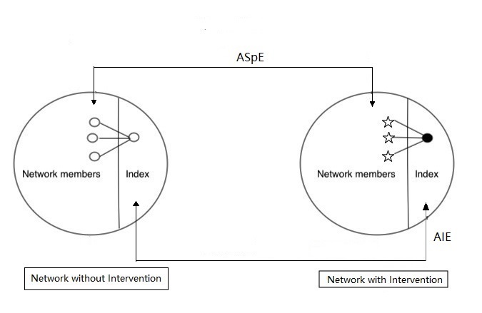
Figure 6: Egonetwork-based design and subsets of data used for the identification of each effect using models (31) and (32) in Section 7.9.1

Remark: Compare to the regression model proposed in main text (we call it single regression model here), the alternative regression model proposed here has more freedom to modelling the observed data since we can make different assumptions to $\epsilon_{1k}$ and $\epsilon_{ik}$. However, for estimating the AIE, the single regression model text exploits the entire individuals in networks without intervention. Thus, for estimating the AIE, the single regression model is more efficient than using (31) only.

7.9.2 Sample Size and Power Calculation

Based on models (31) and (32), and the derived BLUE estimators, we report the hypothesis testing procedures for two hypotheses on the AIE and the ASpE. We then derive the required number of index participants to have adequate power to test the causal effects at a given significant level.

The AIE hypothesis test based on (31) ($HIE_{2}$). Here we want to test the hypothesis of no average individual effect, that is, $H_{0}:\tau=0.$ To test this hypothesis, we rely on the use of the two sided $Z-$test statistc: $Z_{\tau}=\sqrt{K}(\hat{\tau}/\sigma_{\tau})$, where $\sigma^{2}_{\tau}=\sigma^{2}_{Y_{1}}/\{p(1-p)\}$. Using the BLUE estimator of $\theta_{I}$, $Z_{\tau}$ follows a standard normal distribution given the null hypothesis. To against the null hypothesis, the alternative hypothesis, $H_{1}:\tau\neq 0$, represents that $Z_{\tau}$ dose not follow $N(0,1)$ under the alternative hypothesis. Assume that the effect size of $\tau$ is $\Delta_{\tau}$. Given a significant level of the test, $\alpha$, the probability to reject $H_{0}$ when it is true is $P(|Z_{\tau}|>z_{1-\alpha/2}|\tau=0)$ with critical value $z_{1-\alpha/2}$. Then the power of the test is $\text{power}(\Delta_{\tau})=P\{|\sqrt{K}(\hat{\tau}-\Delta_{\tau})/\hat{\sigma}_{\tau})|\geq z_{1-\alpha/2}-\sqrt{K}\Delta_{\tau}/\sigma_{\tau}|Z_{\tau}\sim N(\Delta_{\tau},1)\}=1-\Phi(z_{1-\alpha/2}-\sqrt{K}\Delta_{\tau}/\sigma_{\tau})$, where $\Phi(\cdot)$ is the cumulative distribution function of the standard normal distribution and $z_{\lambda}=\Phi^{-1}(\lambda)$ for any $\lambda\in[0,1]$. Given the required power $1-\lambda$, at significant level $\alpha$, we solve $\text{power}(\Delta_{\tau})$ for $K$ to obtain the required number of index participant of $HIE_{2}$, $K_{\tau}$:

$$K_{\tau}=\frac{\sigma^{2}_{\tau}(z_{1-\alpha/2}+z_{1-\lambda})^{2}}{\Delta_{\tau}^{2}}=\frac{\sigma^{2}_{Y_{1}}(z_{1-\alpha/2}+z_{1-\lambda})^{2}}{p(1-p)\Delta_{\tau}^{2}}$$ (33)

The ASpE hypothesis test based on (32) ($HSpE_{2}$). Here we focus on the hypothesis of no ASpE, $H_{0}:\delta=0$. To test this hypothesis, we use the two-sized Z-test statistic: $Z_{\delta}=\sqrt{K}(\hat{\delta}/\hat{\sigma}_{\delta})$, where

$$\sigma^{2}_{\delta}=\frac{\sigma^{2}_{Y}\{1+(n-1)\rho_{Y}\}}{np(1-p)}.$$

Similar to $HIE_{2}$, $Z_{\delta}$ follows a standard normal distribution given $H_{0}$. Assuming the effect size of $\delta$ is $\Delta$, then given a significant level $\alpha$, the power of the test is $\text{power}(\Delta_{\delta})=1-\Phi(z_{1-\alpha/2}-\sqrt{K}\Delta_{\delta}/\sigma_{\delta})$. We solve $\text{power}(\Delta_{\delta})$ for $K$ to obtain the required number of index participants to achieve a adequate power of the test, $1-\lambda$, given significance level, $\alpha$. To be specific,

$$K_{\delta}=\frac{\sigma^{2}_{\delta}(z_{1-\alpha/2}+z_{1-\lambda})^{2}}{\Delta_{\delta}^{2}}=\frac{\sigma^{2}_{Y}\{1+(n-1)\rho_{Y}\}(z_{1-\alpha/2}+z_{1-\lambda})^{2}}{np(1-p)\Delta_{\delta}^{2}}.$$ (34)

The required number of index participants for testing the AIE and the ASpE simultaneously with power $1-\lambda$ is defined to be $\max(K_{\tau},K_{\delta})$ at significant level $\alpha$, which is the maximum value of $K_{\tau}$ and $K_{\delta}$.

7.9.3 Numerical Simulations

From (33) and (34), we observe that $K_{{\tau}}$ is related to the probability of index treatment $p$ and the effect size $\Delta_{\tau}$, while $K_{{\delta}}$ is related to $p$, the network size $n$, the intra-class correlation $\rho_{Y}$, and the effect size $\Delta_{\delta}$. In particular, we can see that smaller effect size $\Delta_{\tau}$ inflates the required number of index participants, and $K_{\delta}$ increase with $\rho_{Y}$ and decrease with $n$. smaller effect size $\Delta_{\delta}$ also inflates the required samples size of index participants for testing the ASpE.

We fix $\sigma^{2}_{Y_{1}}$, $\sigma^{2}_{Y}$, $\Delta_{\tau}$ and $\Delta_{\delta}$ at 1, while we let $\rho_{Y}$ vary from 0 to 1, $n\in\{1,2,5,8,10\}$, and $p=c(0.3,0.5,0.7,0.9)$. Figure 7 shows the required number of networks for $HIE_{2}$ and $HSpE_{2}$ with $\alpha=5\%$ and $1-\lambda=80\%$. As we can see, for each $p$, the patterns of $K_{\tau}$ and $K_{\delta}$ with $\rho_{Y}$ and $n$ are displayed as we expected. $K_{\tau}$ only changes with $p$, and the optimal value of $p$ is 0.5. Given $p$ and $n$, $K_{\delta}$ increases with $\rho_{Y}$. Smaller $n$ inflates $K_{\delta}$.

Figure 7: Required number of index participants for testing the AIE and ASpE given different value of $p$: $\Delta_{\tau}=\Delta_{\delta}=1$, $\sigma^{2}_{Y_{1}}=\sigma^{2}_{Y}=1$. The line with two colors represents that the two lines of $K_{\tau}$ and $K_{\delta}$ overlap with each other.

7.9.4 Derivations of Variance for Alternative Regression-based Estimators

In Section 7.9.1, we know that $\text{Var}(\hat{\beta}_{I})=\sigma^{2}_{Y_{1}}U^{-1}_{Dk}$, where

$$U_{Dk}=\mathbf{Z}^{\prime}_{1}\mathbf{Z}_{1}=\begin{bmatrix}K&\sum\limits^{K}_{k=1}Z_{1k}\\ \sum\limits^{K}_{k=1}Z_{1k}&\sum\limits^{K}_{k=1}Z^{2}_{1k}\end{bmatrix}.$$

We define $U_{D}=\lim_{K\to\infty}U_{Dk}/K$, then

$$U_{D}=\lim_{K\to\infty}\frac{1}{K}\begin{bmatrix}K&\sum\limits^{K}_{k=1}Z_{1k}\\ \sum\limits^{K}_{k=1}Z_{1k}&\sum\limits^{K}_{k=1}Z^{2}_{1k}\end{bmatrix}=\begin{bmatrix}1&p\\ p&p\end{bmatrix},$$

where we applied the properties: $\lim_{K\to\infty}\sum\limits^{K}_{k=1}Z_{1k}/K=p$ and $\lim_{K\to\infty}\sum\limits^{K}_{k=1}Z^{2}_{1k}/K=p$. As a result,

$$\Sigma_{D}=\lim_{K\to\infty}\sigma^{2}_{Y_{1}}(U_{Dk}/K)^{-1}=\sigma^{2}_{Y_{1}}U^{-1}_{D}=\frac{\sigma^{2}_{Y_{1}}}{p(1-p)}\begin{bmatrix}1&p\\ p&p\end{bmatrix}.$$

Similarly, we have $\text{Var}(\hat{\beta}_{II})=\sigma^{2}_{Y}U^{-1}_{Sk}$ with

$$U_{Sk} =\sum\limits^{K}_{k=1}\mathbf{G}^{\prime}_{Sk}V^{-1}_{Sk}\mathbf{G}_{Sk}=cS_{k}+dT_{k},$$

where $S_{k}=\sum\limits^{K}_{k=1}\mathbf{G}^{\prime}_{Sk}\mathbf{G}_{Sk}$ and $T_{k}=\sum\limits^{K}_{k=1}\mathbf{G}^{\prime}_{Sk}J_{n}\mathbf{G}_{Sk}$. Then with the properties: $\lim_{K\to\infty}\sum\limits^{K}_{k=1}G_{ik}/K=p$ and $\lim_{K\to\infty}\sum\limits^{K}_{k=1}G^{2}_{ik}/K=p$

$$S =\lim_{k\to\infty}\frac{1}{K}S_{k}=\lim_{k\to\infty}\frac{1}{K}\sum\limits^{K}_{k=1}\mathbf{G}^{\prime}_{Sk}\mathbf{G}_{Sk}$$

$$=\lim_{k\to\infty}\frac{1}{K}\sum\limits^{K}_{k=1}\begin{bmatrix}n&\sum\limits^{n+1}_{i=2}G_{ik}\\ =\sum\limits^{n+1}_{i=2}G_{ik}&\sum\limits^{n+1}_{i=2}G^{2}_{ik}\end{bmatrix}$$

$$=\begin{bmatrix}n&np\\ np&np\end{bmatrix}$$

and

$$T =\lim_{k\to\infty}\frac{1}{K}T_{k}=\lim_{k\to\infty}\frac{1}{K}\sum\limits^{K}_{k=1}\mathbf{G}^{\prime}_{Sk}J_{n}\mathbf{G}_{Sk}$$

$$=\lim_{k\to\infty}\frac{1}{K}\sum\limits^{K}_{k=1}\begin{bmatrix}n^{2}&n\sum\limits^{n+1}_{i=2}G_{ik}\\ n\sum\limits^{n+1}_{i=2}G_{ik}&(\sum\limits^{n+1}_{i=2}G_{ik})(\sum\limits^{n+1}_{i=2}G_{ik})\end{bmatrix}$$

$$=\begin{bmatrix}n^{2}&n^{2}p\\ n^{2}p&n^{2}p\end{bmatrix}.$$

We define $U_{S}=\lim_{K\to\infty}U_{Sk}/K$ and recall that $c=1/(1-\rho_{Y})$ and $d=-\rho_{Y}/[1-\rho_{Y}\{1+(n-1)\rho_{Y}\}]$. Then

$$U_{S} =\lim_{K\to\infty}cS_{k}+dT_{k}=cS+dT$$

$$=\left(\frac{n}{1-\rho_{Y}}-\frac{\rho_{Y}n^{2}}{(1-\rho_{Y})\{1+(n-1)\rho_{Y}\}}\right)\begin{bmatrix}1&p\\ p&p\end{bmatrix}$$

and

$$U^{-1}_{S} =\left(\frac{n}{1-\rho_{Y}}-\frac{\rho_{Y}n^{2}}{(1-\rho_{Y})\{1+(n-1)\rho_{Y}\}}\right)^{-1}\frac{1}{p(1-p)}\begin{bmatrix}p&-p\\ -p&1\end{bmatrix}$$

$$=\frac{1+(n-1)\rho_{Y}}{n}\frac{1}{p(1-p)}\begin{bmatrix}p&-p\\ -p&1\end{bmatrix}.$$

As a result, we have

$$\Sigma_{S} =\lim_{K\to\infty}\sigma^{2}_{Y}(U_{Sk}/K)^{-1}$$

$$=\sigma^{2}_{Y}U^{-1}_{S}$$

$$=\sigma^{2}_{Y}\frac{1+(n-1)\rho_{Y}}{np(1-p)}\begin{bmatrix}p&-p\\ -p&1\end{bmatrix}.$$

References

- Aronow and Samii (2017) Aronow, P. M. and C. Samii (2017). Estimating average causal effects under general interference, with application to a social network experiment. The Annals of Applied Statistics 11, 1912–1947.
- Baird et al. (2018) Baird, S., J. A. Bohren, C. McIntosh, and B. Özler (2018). Optimal design of experiments in the presence of interference. Review of Economics and Statistics 100, 844–860.
- Brookes et al. (2004) Brookes, S., E. Whitely, M. Egger, G. Smith, P. Mulheran, and T. Peters (2004). Subgroup analyses in randomized trials: risks of subgroup-specific analyses: power and sample size for the interaction test. J Clin Epidemiol 57, 229–236.
- Buchanan et al. (2018) Buchanan, A. L., S. H. Vermund, S. R. Friedman, and D. Spiegelman (2018). Assessing individual and disseminated effects in network-randomized studies. American journal of epidemiology 187, 2449–2459.
- Cox (1958) Cox, D. R. (1958). Planning of Experiments. New York:Wiley.
- Davey-Rothwell et al. (2011) Davey-Rothwell, M., K. Tobin, C. Yang, C. Sun, and C. Latkin (2011, 04). Results of a randomized controlled trial of a peer mentor hiv/sti prevention intervention for women over an 18 month follow-up. AIDS and behavior 15, 1654–63.
- Donner and Klar (2000) Donner, A. and N. Klar (2000). Design and analysis of cluster randomization trials in health research. London: Arnold.
- Forastiere et al. (2020) Forastiere, L., E. M. Airoldi, and F. Mealli (2020). Identification and estimation of treatment and interference effects in observational studies on networks. Journal of the American Statistical Association, 1–18.
- Halloran and Hudgens (2016) Halloran, M. E. and M. G. Hudgens (2016). Dependent happenings: A recent methodological review. Current Epidemiology Reports 3, 297–305.
- Hayes and Moulton (2009) Hayes, R. J. and L. H. Moulton (2009). Cluster randomised trials. New York: Chapman and Hall/CRC.
- Hemming et al. (2017) Hemming, K., S. Eldridge, G. Forbes, C. Weijer, and M. Taljaard (2017). How to design efficient cluster randomised trials. BMJ 358.
- Hernán and Robins (2020) Hernán, M. and J. Robins (2020). Causal Inference: What If. Boca Raton: Chapman and Hall/CRC.
- Hudgens and Halloran (2008) Hudgens, M. G. and M. E. Halloran (2008). Towards causal inference with interference. Journal of the American Statistical Association 103, 832–842.
- Jiang et al. (2022) Jiang, Z., K. Imai, and A. Malani (2022). Statistical inference and power analysis for direct and spillover effects in two-stage randomized experiments. Biometrics n/a(n/a), 1–12.
- Latkin et al. (2009) Latkin, C., D. Donnell, D. M. S. Sherman, A. Aramrattna, A. Davis-Vogel, V. M. Quan, S. Gandham, T. Vongchak, T. Perdue, and D. Celentano (2009). The efficacy of a network intervention to reduce hiv risk behaviors among drug users and risk partners in chiang mai, thailand and philadelphia, usa. Social science and medicine 68, 740–748.
- Lee et al. (2022) Lee, T., A. L. Buchanan, K. N. V., L. Forastiere, M. E. Halloran, S. R. Friedman, and G. Nikolopoulos (2022). Estimating causal effects of non-randomized hiv prevention interventions with interference in network-based studies among people who inject drugs. Annals of Applied Statistics. In Press 1.
- Leung (2020) Leung, M. P. (2020). Treatment and spillover effects under network interference. Review of Economics and Statistics 102, 368–380.
- Liu and Hudgens (2014) Liu, L. and M. G. Hudgens (2014). Large sample randomization inference of causal effects in the presence of interference. Journal of the American Statistical Association 109, 288–301.
- Liu et al. (2016) Liu, L., M. G. Hudgens, and S. Becker-Dreps (2016). On inverse probability-weighted estimators in the presence of interference. Biometrika 103, 829–842.
- Loh et al. (2018) Loh, W., M. Hudgens, J. Clemens, M. Ali, and M. Emch (2018). Randomization inference with general interference and censoring. Biometrics 76, 235–245.
- Manatunga et al. (2001) Manatunga, A. K., M. G. Hudgens, and S. Chen (2001). Sample size estimation in cluster randomized studies with varying cluster size. Biometrical Journal: Journal of Mathematical Methods in Bioscience 43, 75–86.
- Murray (1998) Murray, D. (1998). Design and Analysis of Group-Randomized Trials. New York, NY: Oxford University Press.
- Ogburn et al. (2017) Ogburn, E., O. Sofrygin, I. Diaz, and M. Laan (2017). Causal inference for social network data. arXiv preprint arXiv:1705.08527.
- Perez‐Heydrich et al. (2014) Perez‐Heydrich, C., M. G. Hudgens, M. E. Halloran, J. D. Clemens, M. Ali, and M. E. Emch (2014). Assessing effects of cholera vaccination in the presence of interference. Biometrics 70, 731–741.
- Perry et al. (2018) Perry, B. L., B. A. Pescosolido, and S. P. Borgatti (2018). Egocentric network analysis: Foundations, methods, and models. Cambridge university press.
- Raudenbush (1997) Raudenbush, S. W. (1997). Statistical analysis and optimal design for cluster randomized trials. Psychological methods 2, 173–185.
- Rosenbaum (2007) Rosenbaum, P. R. (2007). Interference between units in randomized experiments. Journal of the American Statistical Association 102, 191–200.
- Ross (1916) Ross, R. (1916). An application of the theory of probabilities to the study of a priori pathometry.—part i. Proceedings of the Royal Society of London. Series A, Containing papers of a mathematical and physical character 92, 204–230.
- Rubin (1974) Rubin, B. D. (1974). Estimating causal effects of treatments in randomized and non randomized studies. Journal of Educational Psychology 66, 688–701.
- Shieh (2009) Shieh, G. (2009). Detecting interaction effects in moderated multiple regression with continuous variables power and sample size considerations. Organizational Research Methods 12, 510–528.
- Sinclair et al. (2012) Sinclair, B., M. McConnell, and D. P. Green (2012). Detecting spillover effects: Design and analysis of multilevel experiments. American Journal of Political Science 56, 1055–1069.
- Sofrygin and van der Laan (2016) Sofrygin, O. and M. van der Laan (2016). Semi-parametric estimation and inference for the mean outcome of the single time-point intervention in a causally connected population. Journal of Causal Inference 5.
- Sävje et al. (2021) Sävje, F., P. M. Aronow, and M. G. Hudgens (2021). Average treatment effects in the presence of unknown interference. The Annals of Statistics 49, 673–701.
- Tchetgen Tchetgen et al. (2020) Tchetgen Tchetgen, E. J., I. R. Fulcher, and I. Shpitser (2020). Auto-g-computation of causal effects on a network. Journal of the American Statistical Association 116, 833–844.
- Tchetgen Tchetgen and VanderWeele (2012) Tchetgen Tchetgen, E. J. and T. J. VanderWeele (2012). On causal inference in the presence of interference. Statistical Methods in Medical Research 21, 55–75.
- Tian et al. (2022) Tian, Z., D. Esserman, G. Tong, O. Blaha, J. Dziura, P. Peduzzi, and F. Li (2022). Sample size calculation in hierarchical 2× 2 factorial trials with unequal cluster sizes. Statistics in Medicine 41, 645–664.
- Tobin et al. (2010) Tobin, K., S. Kuramoto, M. Davey-Rothwell, and C. Latkin (2010, 11). The step into action study: A peer-based, personal risk network-focused hiv prevention intervention with injection drug users in baltimore, maryland. Addiction (Abingdon, England) 106, 366–75.
- Walters et al. (2019) Walters, S. J., R. M. Jacques, I. B. dos Anjos Henriques-Cadby, J. C. N. Totton, and M. T. S. Xian (2019). Sample size estimation for randomised controlled trials with repeated assessment of patient-reported outcomes: what correlation between baseline and follow-up outcomes should we assume? Trials 20, 1–16.
- Wittes (2002) Wittes, J. (2002). Sample size calculations for randomized controlled trials. Epidemiologic reviews 24, 39–53.
- Yang et al. (2020) Yang, S., F. Li, M. A. Starks, A. F. Hernandez, R. J. Mentz, and K. R. Choudhury (2020). Sample size requirements for detecting treatment effect heterogeneity in cluster randomized trials. Statistics in Medicine 39, 4218–4237.