To Study the Effect of Boundary Conditions and Disorder in Spin Chain Systems Using Quantum Computers

Condensed matter physics plays a crucial role in modern scientific research and technological advancements, providing insights into the the behavior of materials and their fundamental properties. Understanding complex phenomena and systems in condensed matter physics pose significant challenges due to their inherent intricacies. Over the years, computational approaches have been pivotal in unraveling the mysteries of condensed matter physics, but they face limitations when dealing with large-scale systems and simulating quantum effects accurately. Quantum simulation and quantum computation techniques have emerged as promising tools for addressing these limitations, offering the potential to revolutionize our understanding of condensed matter physics. In this paper, we focus on the simulation of Anderson localization in the Heisenberg spin chain systems and explore the effects of disorder on closed and open chain systems using quantum computers.

I Introduction

Condensed matter physics investigates the properties and behaviors of materials in various phases, ranging from solids and liquids to complex electronic systems[1]. The understanding of condensed matter physics has played a pivotal role in enabling significant advancements in nanotechnology, superconductivity[2], and quantum information processing[3]. Despite the remarkable progress made in the field, understanding complex phenomena in condensed matter physics remains a challenging task. These systems often exhibit emergent behavior, where collective interactions between a large number of particles give rise to novel properties. The interplay between different energy scales, the presence of quantum fluctuations, and the effect of disorder complicate the theoretical description of these systems[4] . Conventional computational techniques face limitations in efficiently simulating such complex systems, hindering our ability to comprehend their intricate behavior.

Various computational techniques[5, 6] have been employed to study complex problems in condensed matter physics. Classical numerical methods, such as Monte Carlo simulations[7] and density functional theory[24], have been widely used. While these techniques have provided valuable insights, they are often limited in their ability to handle large-scale systems or accurately capture quantum effects. This necessitates exploring innovative computational approaches, such as quantum simulation and quantum computation [28].

Quantum simulation[29] involves emulating the behavior of quantum systems using other controllable quantum systems, enabling the study of complex quantum phenomena that are challenging to analyze classically. Quantum computation, on the other hand, leverages quantum mechanical principles to perform computations more efficiently than classical computers in certain cases. By harnessing the principles of superposition, entanglement, quantum interference, quantum systems can potentially simulate and compute complex quantum phenomena with unprecedented accuracy and efficiency[30].Quantum systems possess unique properties that make them suitable for simulating complex phenomena in condensed matter physics. These systems can exhibit long-range entanglement, allowing for the exploration of quantum correlations that play a vital role in understanding materials’ properties. Moreover, quantum simulators can be engineered to mimic specific Hamiltonian and explore quantum phase transitions, quantum magnetism, and quantum transport phenomena[31]. The realm of quantum computers opens up exciting possibilities, as their capacity to execute quantum algorithms grant them the potential to efficiently tackle complex problems.

Several companies[12, 13, 14] are actively involved in the development of quantum computing technologies. IBM Quantum is one of the industry leaders, offering researchers and developers access to quantum processors and software tools through the IBM Quantum Experience platform.IBM Quantum has made significant progress in recent years, advancing the capabilities and accessibility of quantum computing. The platform provides cloud-based access to a range of quantum processors, allowing researchers to design and execute quantum simulations. IBM Quantum has continually improved the coherence and connectivity of their quantum processors, enabling more complex simulations and computations. Moreover, the platform offers a suite of programming tools and software development kits (SDKs) to facilitate the implementation of quantum algorithms.

This research paper aims to investigate the phenomenon of Anderson localization in Heisenberg spin chain systems using quantum simulation and computation techniques. Anderson localization[15, 16] refers to the absence of electronic transport in disordered systems, which has significant implications for condensed matter physics. The the study focuses on the effect of defects on both closed and open chain systems, shedding light on the behavior of quantum particles in disordered environments. Quantum simulation methods provide a powerful tool for studying such complex phenomena, and this paper presents a comprehensive analysis of the results obtained through simulations on IBM’s quantum processors.

II Results

Consider N spins 1/2 system, initially prepared in either $|\downarrow\downarrow\downarrow\uparrow\uparrow\uparrow>$ or Néel state$|\uparrow\downarrow\uparrow\downarrow\uparrow>$. The evolution of time will be dictated by a Hamiltonian characterized by the following form:

$$H_{1/2}=-g_{xy}\sum_{k=1}^{m-1}\left(\sigma_{k}^{x}\sigma_{k+1}^{x}+\sigma_{k}^{y}\sigma_{k+1}^{y}\right)+\sum_{k=1}^{m}\left(h_{k}\sigma_{k}^{z}\right)$$ (1)

with $g_{xy}>0$ represents nearest neighbor interaction between $x(\sigma^{x})$ and $y(\sigma^{y})$ spins whereas $h_{k}$ represents an external field that couples to Z-spins at site $k$ and $\sigma_{k}^{\alpha}$ are the Pauli matrices with eigenvalues ±1.

On basis of parameter $h_{k}\neq 0$, we get following spin chain system. Disordered $XX$ chain for $g_{xy}>0$ and $h_{k}$ where $h_{k}=[-h,h]$. The observable of interest is staggered magnetization, which is defined as

$$M_{s}(t)=\frac{1}{m}\sum_{k}(-1)^{k}<\sigma_{k}^{z}>$$ (2)

Here $m$ is the number of qubits. The choice of this observable is necessitated by the realization that for a system with long range antiferromagnetic order, the staggered magnetization is non-zero and can be treated as the order parameter. Fortunately, $M_{s}(t)$ is in $z-basis$, so we only need post-process calculations on measured qubits to compute the staggered magnetization. The expectation value of spin operator Pauli-Z has value 1 for state $|0>$ and value 0 for state $|1>$. After measuring the qubit at the quantum back end, we map the qubit with state $|0>$ to a value 1 and qubit with state $|1>$ to a value of 1 to find the required observable which is staggered magnetization in our case.

To simulate many body systems, IBM makes available different types of simulators. Some of them are noise-free while others have noise errors. In this regard, Aer is an ideal simulator with zero noise while qasm simulator has some noise errors. We will compare the results obtained on the quantum computer with those from qasm simulator.

First of all Consider the disorder $XX$ chain, $H_{1/2}=-g_{xy}\sum_{k=1}^{m-1}\left(\sigma_{k}^{x}\sigma_{k+1}^{x}+\sigma_{k}^{y}\sigma_{k+1}^{y}\right)+\sum_{k=1}^{m}\left(h_{k}\sigma_{k}^{z}\right)$ with $g_{xy}>0$ and $h_{k}=0$ and a Neel state $\psi(t=0)=|\downarrow\uparrow\downarrow\uparrow>$ as an initial state to compute the staggered magnetization to predict the behavior of the system.

As the expectation value of spin operator Pauli-Z has value 1 for state $|\uparrow>$

$$\sigma_{z}|\uparrow>=1|\uparrow>$$

and value -1 for state $|\downarrow>$

$$\sigma_{z}|\downarrow>=-1|\downarrow>.$$

From Eqn.(2) and for Neel state $\psi(t=0)=|\downarrow\uparrow\downarrow\uparrow>$, the staggered magnetization $M_{s}(t=0)$

$$M_{s}(t=0)=\frac{1}{m}\sum_{k}(-1)^{k}<\sigma_{k}^{z}>$$ (3)

$$M_{s}(t=0)=\frac{1}{4}[(-1)^{1}<\downarrow\uparrow\downarrow\uparrow|\sigma_{z}^{1}|\downarrow\uparrow\downarrow\uparrow>+(-1)^{2}<\downarrow\uparrow\downarrow\uparrow|\sigma_{z}^{2}|\downarrow\uparrow\downarrow\uparrow>$$

$$+(-1)^{3}<\downarrow\uparrow\downarrow\uparrow|\sigma_{z}^{3}|\downarrow\uparrow\downarrow\uparrow>+(-1)^{4}<\downarrow\uparrow\downarrow\uparrow|\sigma_{z}^{4}|\downarrow\uparrow\downarrow\uparrow>]$$

$$M_{s}(t=0)=\frac{1}{4}\left[(-1)^{1}(-1)+(-1)^{2}(1)+(-1)^{3}(-1)+(-1)^{4}(1)\right]$$

$$M_{s}(t=0)=\frac{1}{4}\left[1+1+1+1\right]$$

$$M_{s}(t=0)=1$$

Hence we expect $M_{s}(t=0)$=1 , where the initial state is Neel state.

For the disorder $XX$ chain the Hamiltonian is given as

$$H_{1/2}=-g_{xy}\sum_{k=1}^{m-1}\left(\sigma_{k}^{x}\sigma_{k+1}^{x}+\sigma_{k}^{y}\sigma_{k+1}^{y}\right)+\sum_{k=1}^{m}\left(h_{k}\sigma_{k}^{z}\right)$$

At later times ($t>0$), the initial state will evolve under the $XX$ Hamiltonian given above. The staggered magnetization will no longer have its initial value of 1 because the orientation of spins will no longer be purely along the $z-axis$ but will begin to orient in the $x-y$ plane. Hence staggered magnetization will approach zero at later times.

II-A Effect of Disorder $h_{k}$ and Boundary Condition

II-A1 Open Chain

The Hamiltonian in given as

$$H_{1/2}=-g_{xy}\sum_{k=1}^{m-1}\left(\sigma_{k}^{x}\sigma_{k+1}^{x}+\sigma_{k}^{y}\sigma_{k+1}^{y}\right)+\sum_{k=1}^{m}\left(h_{k}\sigma_{k}^{z}\right)$$

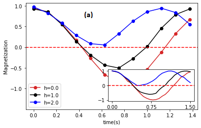
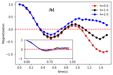
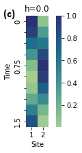
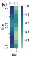
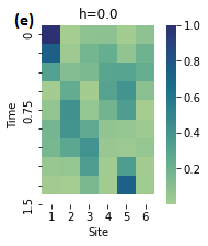
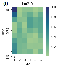
Figure 1: Disordered $XX$ Open chain system when $g_{xy}=1$ and $h_{k}$. Fig.(a) Magnetization for 2 sites. Fig.(b) Magnetization for 4-sites. Fig.(c-e) Time and Disorder-Dependent Probability for$m=2$ and $m=4$Sites

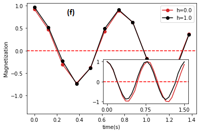
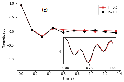
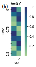
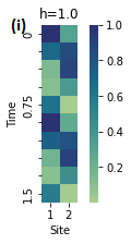
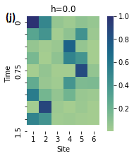
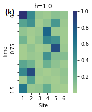
Figure 2: Disordered $XX$ closed chain system when $g_{xy}=1$ and $h_{k}$. Fig.(f) Magnetization for 2 sites. Fig.(g) Magnetization for 4 sites. Fig.(h-k) Time and Disorder-Dependent Probability in a Closed Chain System for $m=2$ and $m=4$Sites

In Fig.(1a and b) we plotted staggered magnetization for different values of $h_{k}$: the black line represent the staggered magnetization for $h_{k}=0.0$, the red line for $h_{k}=0.5$and blue line for $h_{k}=1$. In Fig.(1) the results in a small window were simulated on IBM quantum devices while the solid line with filled circles represents qasm simulator results for $XX$ chain. In the Fig. (1(a)) the $XX$ chain model is simulated for 2-sites and in Fig.(1(b)) for 4-sites. In Fig.(1) we can see that the results of the IBM quantum computer deviate from the qasm simulator as $\delta t>1$ because the available quantum devices have a high error rate and particularly decoherence of qubits is high for longer times. The deviation of the results becomes more noticeable for the 2-site system, as the number of qubits rises, leading to increased decoherence. In all three cases, the magnetization’s time evolution exhibits oscillatory behavior for both the 2-spin and 4-spin systems. The explanation of oscillations in $M_{s}(t)$ has been given above which holds in the presence of disorder. It is well established that disorder leads to Anderson localization in 1D systems such as spin chains under consideration and halts the dynamics. It is expected that relaxation of staggered magnetization $M_{s}(t)$ will be slowed, as seen in our plots and has been observed in recent past research[17]. Upon measuring a quantum system, its state undergoes a collapse, resulting in a single basis vector. The probabilities of obtaining a basis state upon measuring $|\psi(t)>$ are determined by the absolute squares of the coefficients. By analyzing the probability plots, we can validate our predictions regarding the impact of the disorder on the system’s evolution. In Fig.(1(c-f)), we can see that for small values of disorder $h$ and open chain system nearly all states are involved in the dynamics. Additionally, the intermediate states also contribute to the overall behavior of the system. As the value of $h$ increases, the system requires more time to evolve from the initial state |$\downarrow\uparrow$⟩ to the final state $|\uparrow\downarrow\rangle$ and similarly, for four spin system, the system requires more time to evolve from the initial state $|\downarrow\uparrow\downarrow\uparrow>$ to the final state $|\uparrow\downarrow\uparrow\downarrow>$. While for the high value of disorder $h$, the probability of the intermediate states will decrease and approaches zero. This implies that these intermediate states are merely virtual states and not physically realized in this particular case. They play a theoretical role in the dynamics but do not manifest as observable outcomes.

II-A2 Closed Chain

If we have a closed chain rather than an open chain, then the system takes less time to evolve from the first state to the last state no matter how large disorder $h_{k}$ is. This is so because now there are two choices to get from the first state to last in case of closed chain. It is well established that disorder leads to Anderson’s localization in 1D systems but for closed chain the system is not localized as shown in the Fig.(2).

III Quantum Circuit

III-A Quantum Bit

The qubit state is given as

$|0>=\left(\begin{array}[]{c}1\\ 0\end{array}\right)$                           $|1>=\left(\begin{array}[]{c}0\\ 1\end{array}\right)$

We can visualization qubit states $|0>$and $|1>$ with the help of Bloch sphere:

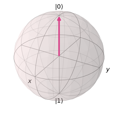
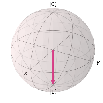
Figure 3: Qubit States$|0>$ and $|1>$ on Bloch Sphere

III-B Superposition

Quantum bits are different from classical bits in terms of allowed states.Classical bits can have only two states $|0>$ and $|1>$ but quantum mechanics allows the qubit to take any value which is a coherent superposition of $|0>$ and $|1>$ states.Hence, a qubit can be expressed as a superposition[10], a combination of both |0| and |1| states, as elucidated in reference. For instance,

$$|a>=\frac{1}{\sqrt{2}}(|0>+|1>)$$ (4)

In the above state the probability of state $|0>$ and $|1>$ are equal which is $\frac{1}{2}$. On a Bloch sphere the state $|a>$ is represented as

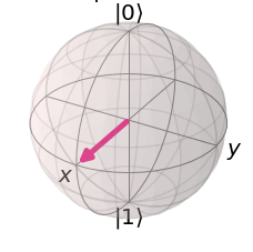
Figure 4: Superposition of state $|0>$ and $|1>$ with equal probability on Bloch Sphere

By using the superposition of $|0>$ and $|1>$ state we can also define a number of different states which will be useful when we discuss complex circuits:

$$|b>=\frac{1}{\sqrt{2}}(|0>-|1>)\qquad|c>=\frac{1}{\sqrt{2}}(|0>+\iota|1>$$

$$|d>=\frac{3}{\sqrt{4}}(|0>+\sqrt{\frac{1}{4}}|1>)\qquad|e>=\frac{\sqrt{3}}{2}(|0>+\frac{\iota-1}{\sqrt{8}}|1>)$$

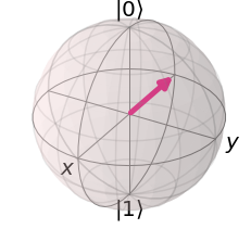
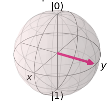
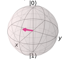
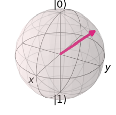
Figure 5: Superposition states $|b>$,$|c>$, $|d>$ and $|e>$ on Bloch sphere

The details of how we can measure single and multiple qubit states are given in Appendix I.

III-C Gates

First, we discuss Pauli gates

$\sigma^{x}=\left(\begin{array}[]{cc}0&1\\ 1&0\end{array}\right)$$\hskip 5.69046pt\sigma^{y}=\left(\begin{array}[]{cc}0&-\iota\\ \iota&0\end{array}\right)\hskip 5.69046pt$$\sigma^{z}=\left(\begin{array}[]{cc}1&0\\ 0&-1\end{array}\right)$

Pauli x gate rotate the state by$180^{o}$, y gate is a combination of bit-flip and phase flip and z-gate only flips the phase.

Figure 6: Pauli X, Y and Z gates

Using rotation gates, we have the ability to rotate a state by an angle $\phi$ around the$x,y,$or$z-axis,$ thereby obtaining the rotated state. The following rotation gates implement rotations about the $x,y,$ and $z-axis$:

$R^{x}(\phi)=e^{-i\frac{\phi\sigma^{x}}{2}}$  $R^{y}(\phi)=e^{-i\frac{\phi\sigma^{y}}{2}}$ $R^{z}(\phi)=e^{-i\frac{\phi\sigma^{z}}{2}}$

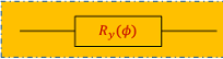
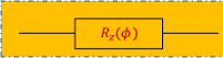
Figure 7: Rotation $R^{x}(\phi),R^{y}(\phi)$ and $R^{z}(\phi)$ gates

The Hadamard gate is a single-qubit gate, defined as follows as:

$$H=\frac{1}{\sqrt{2}}\left(\begin{array}[]{cc}1&1\\ 1&-1\end{array}\right)$$

Hadamard gate acting on either $|0>$ or $|1>$ state creates a state which is an equal superposition of $|0>$ and $|1>$. This will turn out to be very useful in quantum computation.

$H|0>=\frac{1}{\sqrt{2}}(|0>+|1>)\hskip 14.22636pt$$H|1>=\frac{1}{\sqrt{2}}(|0>-|1>)$

Another improtant single qubit gate is phase gate. It will only change the phase of the state either apply on $|0>$ or $|1>$

$$S=\left(\begin{array}[]{cc}1&0\\ 0&e^{i\lambda}\end{array}\right)$$

Figure 8: Circuit for Hadamard and Phase gate

The first multi qubit gate is $CNOT$ gate but we can reverse the $CNOT$ gate by applying circuit as shown in fig(9)

$CNOT=\left(\begin{array}[]{cccc}1&0&0&0\\ 0&1&0&0\\ 0&0&0&1\\ 0&0&1&0\end{array}\right)$

$RCNOT=\left(\begin{array}[]{cccc}1&0&0&0\\ 0&0&0&1\\ 0&0&1&0\\ 0&1&0&0\end{array}\right)$

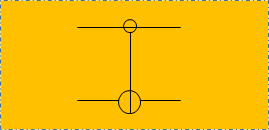
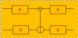
Figure 9: Circuit for $Cnot$ and $RCnot$ gates

IV Mathematical model for Simulating Spin chain Hamiltonian

The Hamiltonian for spin chains[21] system is given as

$$H_{1/2}=-g_{xy}\sum_{k=1}^{m-1}\left(\sigma_{k}^{x}\sigma_{k+1}^{x}+\sigma_{k}^{y}\sigma_{k+1}^{y}\right)+\sum_{k=1}^{m}\left(h_{k}\sigma_{k}^{z}\right)$$

As our focus lies in dynamics, specifically the time evolution of states, we construct the time evolution operator

$$e^{-iH_{1/2}t}=\left(e^{-i\left[\sum_{k=1}^{m-1}\left\{-g_{xy}\left(\sigma_{k}^{x}\sigma_{k+1}^{x}+\sigma_{k}^{y}\sigma_{k+1}^{y}\right)+h_{k}\left(h_{k}\sigma_{k}^{z}\right)\right\}\right]t}\right)$$ (5)

we can implement the required operation[22] needed in time evolution operator for the Hamiltonian for spin chain system given in Eqn.(5) as shown in Fig.(10).

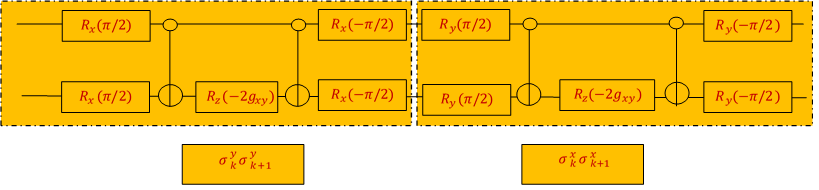
Figure 10: Quantum circuit for the digital quantum simulation of 2-qubit spin chain system

It is well-established that any n-qubit quantum computation can be accomplished using a sequence of one-qubit and two-qubit quantum logic gates. Nevertheless, finding the optimal circuit for a specific family of gates, even for two-qubit gates, is a challenging task. This poses an issue as quantum computation experimentalists can currently only execute a limited number of gate operations within the coherence time of their physical systems. Without an established procedure for optimal quantum circuit design, experimentalists might encounter difficulties in demonstrating certain quantum operations. In Fig.(10) we can see that $6-CNot$ gates are required to solve two-qubit spin chain system while in Fig. (11) which is given below, we can see that $2-CNot$ gates are used to solve 2-qubit spin chain system. Indeed, in this context, we review a procedure for constructing an optimal quantum circuit[23] that enables the realization of a general two-qubit quantum computation. The detail of the procedure is given in Appendix II.

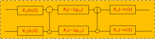
Figure 11: Quantum circuit to implement $e^{i(\sigma_{k}^{x}\sigma_{k+1}^{x}+\sigma_{k}^{y}\sigma_{k+1}^{y})g_{xy}}$

V Trotter Decomposition

To implement time evolution of states governed by $H_{1/2}$numerically, we employ Trotter decomposition.

Using Trotter decomposition[19]

$$e^{-iH_{1/2}t}\approx\left(\prod_{k=1}^{n}e^{-iH_{1/2}\delta t/m}\right)^{m}$$ (6)

where $n$ is a number of terms. As we increase the number of Trotter steps, the results of the Trotter approximation get closer to the desired outcome. However, this improvement comes at the expense of increasing the number of gates, leading to a longer circuit length[20].

Let’s consider a Hamiltonian of the form $H_{1/2}=\hat{O}+\hat{Q}$, where $[\hat{O},\hat{Q}]\neq 0$. Since these operators do not generally commute, we can approximate the time evolution as follows:

$$e^{-iH_{1/2}t}\approx e^{-i\hat{O}t}e^{-i\hat{Q}t}+O(t)$$

This approximation can be naturally extended to Hamiltonian that consists of more than two terms. To utilize this fact for tottered evolution, we can follow the two steps outlined in the main text. Let’s now delve into the details of these steps more thoroughly. For the Hamiltonian

$$H_{1/2}=-g_{xy}\sum_{k=1}^{m-1}\left(\sigma_{k}^{x}\sigma_{k+1}^{x}+\sigma_{k}^{y}\sigma_{k+1}^{y}\right)+\sum_{k=1}^{m}\left(h_{k}\sigma_{k}^{z}\right)$$

and

$$e^{-iH_{1/2}t}=\left(e^{-i\left[\sum_{k=1}^{m-1}\left\{-g_{xy}\left(\sigma_{k}^{x}\sigma_{k+1}^{x}+\sigma_{k}^{y}\sigma_{k+1}^{y}\right)+h_{k}\left(h_{k}\sigma_{k}^{z}\right)\right\}\right]t}\right)$$

We first define the operators

$\hat{O_{k}}=e^{-ih_{k}\sigma_{k}^{z}\delta t}$, $\hat{Q_{k}}=e^{-i(-g_{xy}(\sigma_{k}^{x}\sigma_{k+1}^{x}+\sigma_{k}^{y}\sigma_{k+1}^{y}))\delta t}$

Using $\hat{O_{k}}$ and$\hat{Q_{k}}$

$$e^{-i\hat{Ht}}\approx\left(\prod_{k}\hat{O_{k}}\right)\left(\prod_{k=even}\hat{Q_{k}}\right)\left(\prod_{k=odd}\hat{Q_{k}}\right)+O(\delta t)$$ (7)

which shown in the Fig.(12).

For $4$ sites

$$\prod_{k}O_{k}=\left(e^{-ih_{1}\sigma_{1}^{z}\delta t}\right)\left(e^{-ih_{2}\sigma_{2}^{z}\delta t}\right)\left(e^{-ih_{3}\sigma_{3}^{z}\delta t}\right)\left(e^{-ih_{4}\sigma_{4}^{z}\delta t}\right)$$

For $k$ is even

$$\prod_{k=even}\hat{Q}=e^{ig_{xy}(\sigma_{2}^{x}\sigma_{3}^{x}+\sigma_{3}^{y}\sigma_{4}^{y}))\delta t}$$

For $k$ is odd

$$\prod_{k=odd}\hat{Q}=\left(e^{ig_{xy}(\sigma_{1}^{x}\sigma_{2}^{x}+\sigma_{1}^{y}\sigma_{2}^{y})\delta t}\right)\left(e^{ig_{xy}(\sigma_{3}^{x}\sigma_{4}^{x}+\sigma_{3}^{y}\sigma_{4}^{y})\delta t}\right)$$

Quantum circuit to implement Eqn.(7) operation is shown in Fig.(12)

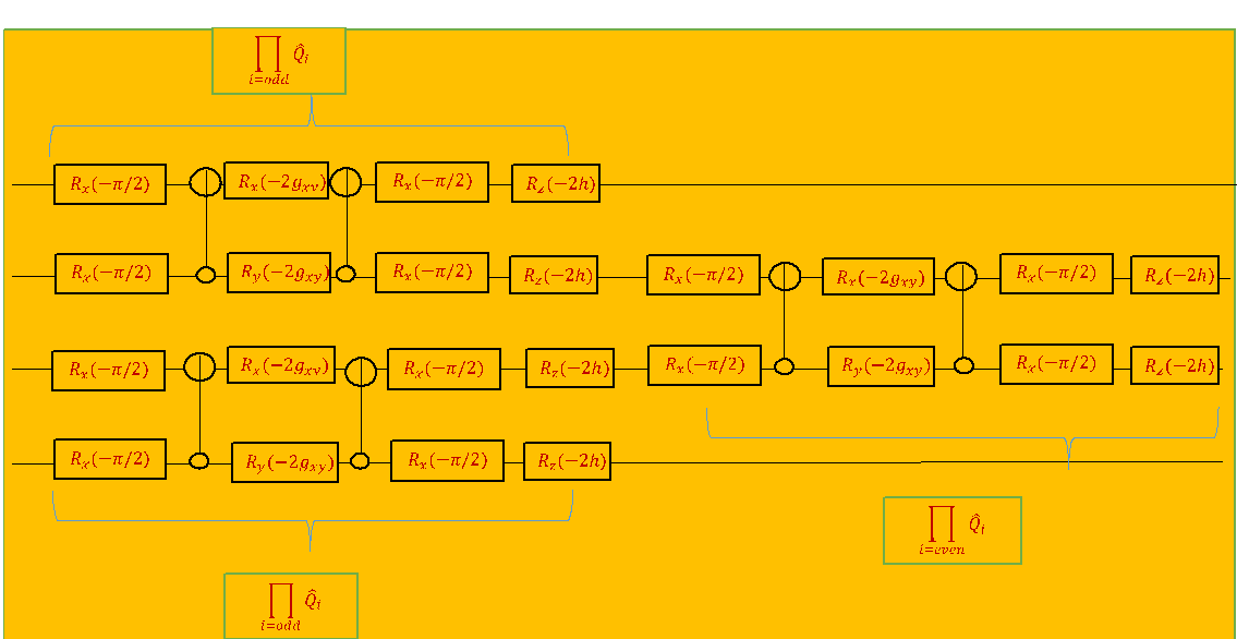
Figure 12: Disordered $XX$ chain for $g_{xy}=1$ and $h_{k}$ where $h_{k}=[-h,h]$.

The detail of the algorithm to implement the circuit on IBM quantum experience is given in

VI Error Analysis

In this paper, we have determined the time evolution of many-body states of spin chains by employing quantum algorithms run on IBM quantum computers. Currently, IBM quantum devices have noise errors due to multi-qubit gates and decoherence of qubits so on an hourly basis these machines are calibrated; that is why the results and data obtained at certain times may have high error rates as compared to other times/days. So the real-time data of different quantum processors can be checked anytime[18].

For the time evolution of an initial state governed by the Hamiltonian and to obtain an observable quantity we calculate the observable which is staggered magnetization. We have discussed two circuits: one is shown in fig(10) which has $4-CNot$ gates and other circuit is shown in fig(11) which has $2-CNot$ gates for the disorder $XX$ chain. The results corresponding to both quantum circuits are shown in Fig.(13)

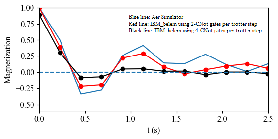
Figure 13: Scheme of quantum circuit using: $4-CNot$ gates(black line) per trotter step and $2-CNot$ gates (orange line) per trotter step

This analysis holds significant importance since one effective method to reduce the error rate is by minimizing the number of gates. Above Fig.(13) the black line represents quantum circuit scheme which is using $4-CNot$ gates in one trotter step and the the orange line represents $2-CNot$ gates in one trotter step while the the blue line shows the results of an ideal simulator named Aer. To have a better comparison we take $12-trotter$ steps for time evolution of states otherwise due to the decoherence of qubits and an error rate of $CNot$ gates the results deviated quickly from ideal results.

Black line: $4-CNot$ gates per trotter step and there are total of 12 steps for time evolution which implies that the total number of $CNot$ gates will be $48$.

Orange line: $2-CNot$ gates per trotter step and there are a total of 12 steps which implies that the total number of $CNot$ gates will be $24$.

We have employed the quantum circuit scheme which has a minimum error due to fewer number of $CNot$ gates. This can be seen from the above graphs since the orange line is closer to the ideal simulation as compared to the black line. Now, we will study the magnetization for three different cases of spin chains by using the quantum circuit which has $(2-CNot)$ gates per trotter step.

Experimental Realization: Studying quantum spin chain systems in a laboratory setting is a challenging exercise because different parameters are present which are difficult to control. Ultra cold atoms in optical lattices have proven to be an invaluable experimental system for investigating spin chain systems. Their unique characteristics allow for precise control and manipulation, offering a high degree of contrast essential for initializing spin systems and studying their dynamics. In this regard, the initialization of the many body spin state, tunability of exchange interaction and time-resolved magnetization have been demonstrated in ultra cold atoms systems(see [25, 26] and reference therein).

Future Outlook: Work presented in this thesis can be extended in several directions. One clear extension, even though more challenging, is the extension of this work to 2D systems, both ferromagnetic and anti-ferromagnetic[28]. Another direction is driven systems such as Floquet systems[29, 30]. As new and improved quantum computers are developed more challenging problems can be attacked. The work carried out in this thesis provides the perfect platform for it.

Appendix I

Measurement

Single Qubit states:

In section 3.2, we have seen the following superposition state of a qubit

$$|b>=\frac{1}{\sqrt{2}}(|0>-|1>).$$ (8)

Figure 14: Qubit state $|b>=\frac{1}{\sqrt{2}}(|0>-|1>)$ lies half way between north and south pole on Bloch sphere.

Quantum mechanics allows states to be superpositions but when we measure a quantum state we get a defined state $|0>$ or $|1>$ with some probability. It means the superposition of qubits collapses to a defined state when we measure it at the end of the computation. For example, in the above qubit $|b>$ , if we measure it we get $|0>$state with probability $1/2$ and $|1>$with probability $1/2$. Geometrically the qubit lies halfway between the north and south pole of the Bloch sphere.

As another example we calculate the probabilities of another qubit:

$$|e>=\frac{\sqrt{3}}{2}(|0>+\frac{\iota-1}{\sqrt{8}}|1>$$

Probability of state $|0>$ is given as

$$|\frac{\sqrt{3}}{2}|^{2}=\frac{3}{4}$$

Probability of state $|1>$ is given as

$$|\frac{\iota-1}{\sqrt{8}}|^{2}=\frac{2}{8}$$

So on measurement $|0>$ is obtained with probability $\frac{3}{4}$ and the probability of $|1>$is $\frac{2}{8}$, which is shown in Fig.(2.4)

Multiple Qubit States:

In section 3.3 we have discussed single qubit states, the superposition of states of single qubits, and how to measure these states. Now we will move towards superposition and measurement of multiple qubits states. In multiple qubits, we write the states of both qubits as a tensor product, for example

$$|0>\otimes|0>)=|00>.$$

For two qubit we get $2^{2}$ states

$$\{|00>,|01>,|10>,|11>\}$$

The matrix representations of these states is

$$|00>=|0>\otimes|0>)=\left(\begin{array}[]{c}1\\ 0\end{array}\right)\otimes\left(\begin{array}[]{c}1\\ 0\end{array}\right)=\left(\begin{array}[]{c}1\\ 0\\ 0\\ 0\end{array}\right)$$

$$|01>=|0>\otimes|1>)=\left(\begin{array}[]{c}1\\ 0\end{array}\right)\otimes\left(\begin{array}[]{c}0\\ 1\end{array}\right)=\left(\begin{array}[]{c}0\\ 0\\ 0\\ 1\end{array}\right)$$

$$|10>=|1>\otimes|0>)=\left(\begin{array}[]{c}0\\ 1\end{array}\right)\otimes\left(\begin{array}[]{c}1\\ 0\end{array}\right)=\left(\begin{array}[]{c}0\\ 0\\ 1\\ 0\end{array}\right)$$

$$|11>=|1>\otimes|1>)=\left(\begin{array}[]{c}0\\ 1\end{array}\right)\otimes\left(\begin{array}[]{c}0\\ 1\end{array}\right)=\left(\begin{array}[]{c}0\\ 0\\ 0\\ 1\end{array}\right).$$

The superposition of these states is given as

$$|\phi_{2_{qubit-states}}>=\alpha_{0}|00>+\alpha_{1}|01>+\alpha_{2}|10>+\alpha_{3}|11>$$ (9)

The probabilities of obtaining qubit states are as follows:

1. Probability of $|00|\text{is }|\alpha_{0}|^{2}$

2. Probability of $|01|\text{is }|\alpha_{1}|^{2}$

3. Probability of |$10|\text{is }|\alpha_{2}|^{2}$

4. Probability of $|11|\text{is}|\alpha_{3}|^{2}$

If we measure only the left qubit $|0>$ the probability is given as $|\alpha_{0}|^{2}+|a_{1}|^{2}$. Allow us to consider an example utilizing the following two-qubit state:

$$|\gamma>=\frac{1}{\sqrt{7}}|00>+\frac{2}{\sqrt{7}}|01>+\frac{3}{\sqrt{7}}|10>+\frac{1}{\sqrt{7}}|11>$$ (10)

The probability of measuring $|0>$ is given as

$$|\frac{1}{\sqrt{7}}|^{2}+|\frac{2}{\sqrt{7}}|^{2}=\frac{3}{7}$$

For three qubit we have $2^{3}$states

$$\{|000>,|010>,|001>,|100>,|110>,|101>,|011>,|111>\}$$

The superposition of these states is given as

$$|\phi_{3_{qubit-states}}>=\beta_{0}|000>+\beta_{1}|010>+\beta_{2}|001>+\beta_{3}|100>$$

$$+\beta_{4}|110>+\beta_{5}|101>+\beta_{6}|011>+\beta_{7}|111>$$

if we measure the qubit state $|000>$ its probability is $|\beta_{0}|^{2}$, the probability of $|010>$ is $|\beta_{1}|^{2}$, the probability of $|001>$ is $|\beta_{2}|^{2}$and so on.

For a system with $m$ qubits, there exist $2^{m}$ states. The superposition state can be expressed as follows:

$$|\phi_{m_{qubit-states}}>=\beta_{0}|000..m>+\beta_{1}|010....m>$$

$$+\beta_{m}|001...m>+..............=\left(\begin{array}[]{c}\beta_{0}\\ \beta_{1}\\ ....\\ ....\\ ....\\ \beta_{m}\end{array}\right)$$

Appendix II

Consider

$$N(\lambda,\gamma,\phi)=e^{i(\lambda\sigma_{k}^{x}\sigma_{k+1}^{x}+\gamma\sigma_{k}^{y}\sigma_{k+1}^{y}+\phi\sigma_{k}^{z}\sigma_{k+1}^{z})}$$

For x and z terms only, $\gamma=0$

$$N(\lambda,0,\phi)=e^{i(\lambda\sigma_{k}^{x}\sigma_{k+1}^{x}+\phi\sigma_{k}^{z}\sigma_{k+1}^{z})}$$

As we have Magic matrix[14]

$$M=\frac{1}{\sqrt{2}}\left(\begin{array}[]{cccc}1&i&0&0\\ 0&0&i&1\\ 0&0&i&-1\\ 1&-i&0&0\end{array}\right)$$

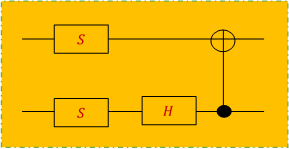
Figure 15: Quantum circuit to implement magic basis

Using this matrix we can find that

$$M^{\dagger}N(\lambda,0,\phi)M=e^{i\phi\sigma^{z}}\otimes e^{i\lambda\sigma^{z}}.$$ (11)

$\implies$

$$N(\lambda,0,\phi)=Me^{i\phi\sigma^{z}}\otimes e^{i\lambda\sigma^{z}}M^{\dagger}$$ (12)

Quantum circuit to implement $Me^{i\phi\sigma^{z}}\otimes e^{i\lambda\sigma^{z}}M^{\dagger}$is shown in Fig.(16)

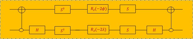
Figure 16: Quantum circuit to implement $N(\lambda,0,\phi)=Me^{i\phi\sigma^{z}}\otimes e^{i\lambda\sigma^{z}}M^{\dagger}$

As $[S,R_{z}(\theta)]=0$ and $HR_{z}(\theta)H=R_{x}(\theta)$. Then circuit reduced to

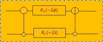
Figure 17: Quantum circuit to implement $N(\lambda,0,\phi)=Me^{i\phi\sigma^{z}}\otimes e^{i\lambda\sigma^{z}}M^{\dagger}$

References

- [1] E. Morosan, D. Natelson, A. H. Nevidomskyy, Qimiao Si, “ Strongly Correlated Materials”, Adv. Mat. 24, 4896-4923 (2012).
- [2] S. Murmann, A. Bergschneider, V. M. Klinkhamer, G. ZÃŒrn, T. Lompe, and S. Jochim, “Two Fermions in a Double Well: Exploring a Fundamental Building Block of the Hubbard Model”, Phys. Rev. 114, 080402 (2015).
- [3] S. Sachdev, “Quantum Phase Transitions”, Cambridge University Press, Cambridge, UK 2011.
- [4] P. A. Lee, N. Nagaosa, and X. G. Wen, “ Doping a Mott insulator: Physics of high-temperature superconductivity”, Rev. Mod. Phys. 78 (2006).
- [5] J. M. Haile, “Molecular Dynamics Simulation: Elementary Methods”, Wiley-Interscience, New York, USA 1992.
- [6] S. Montangero, “Introduction to Tensor Network Methods”, Springer Nature Switzerland AG, Cham, CH 2018.
- [7] J. Gubernatis, N. Kawashima, P. “Werner, Quantum Monte Carlo Methods”, Cambridge University Press, Cambridge, UK 2016.
- [8] M. Georgescu, S. Ashhab, and Franco Nori, “Quantum simulation”, Rev. Mod. Phys. 86, 153 (2014 ).
- [9] Feynman R. Found. Phys. 16, 507(1986).
- [10] M. A. Nielsen, I. L. Chuang, “Quantum computation and quantum information”, Cambridge University Press, Cambridge, UK 2000.
- [11] I. Bloch, J. Dalibard and S. Nascimbene, “Quantum simulations with ultracold quantum gases”, Nat. Phy. 8, 267–276 (2012).
- [12] IBM Quantum Experience. https://www.ibm.com/quantum-computing/technology/experience.
- [13] Google Quantum AI. https://quantumai.google.
- [14] D-wave. https://www.dwavesys.com/learn/quantum-computing.
- [15] Krzysztof Byczuk, Walter Hofstetter and Dieter Vollhardt, “Competition between Anderson Localization and Antiferromagnetism in Correlated Lattice Fermion Systems with Disorder”, Phys. Rev. Lett. 102, 146403 (2009).
- [16] Kramer, B. & MacKinnon, “A. Localization: theory and experiment”, Reports Prog. Phys. 56, 1469–1564 (1993).
- [17] A. Smith, M. S. Kim, F. Pollmann, J. Knolle, “Simulating quantum many-body dynamics on a current digital quantum computer”, Npj Quant. Inf. 5, 106 (2019).
- [18] IBM Quantum Experience. https://quantum-computing.ibm.com/services/resources.
- [19] Andrew M. Childs, Yuan Su, Minh C. Tran, Nathan Wiebe and Shuchen Zhu, “A Theory of Trotter Error”, Phys. Rev. X 11, (2021).
- [20] Andrew Tranter, Peter J. Love, Florian Mintert, Nathan Wiebe, and Peter V. Coveney, “Ordering of Trotterization: Impact on Errors in Quantum Simulation of Electronic Structure”, Entropy. 12, 21(2019).
- [21] Peter Barmettler,Matthias Punk, Vladimir Gritsev, Eugene Demler and Ehud Altman,“Quantum quenches in the anisotropic spin-1 2 Heisenberg chain: different approaches to many-body dynamics far from equilibrium”, New J. Phys. 12, (2010).
- [22] Francesco Tacchino, Alessandro Chiesa, Stefano Carretta and Dario Gerace, “Quantum Computers as Universal Quantum Simulators: State-of-the-Art and Perspectives”, Advanced Quantum Technologies 3, (2020)
- [23] Vatan, F. & Williams, C. “Optimal quantum circuits for general two-qubit gates”, Phys. Rev. A 69, 032315 (2004).
- [24] S. Trotzky, P. Cheinet, S. Fölling, M. Feld, U. Schnorrberger, A. M. Rey, A. Polkovnikov, E. A. Demler, M. D. Lukin, and I. Bloch, “Time-Resolved Observation and Control of Superexchange Interactions with Ultracold Atoms in Optical Lattices”, Science. 319, 295-299 (2008).
- [25] M. Bukov, L. D’Alessio, and A. Polkovnikov, “Universal high-frequency behavior of periodically driven systems: from dynamical stabilization to Floquet engineering”, Adv. Phys. 64, 139 (2015).
- [26] Simon Murmann, Andrea Bergschneider, Vincent M. Klinkhamer, Gerhard ZÃŒrn, Thomas Lompe, and Selim Jochim, “Two Fermions in a Double Well: Exploring a Fundamental Building Block of the Hubbard Model”, Phys. Rev. 114, 080402 (2015).
- [27] E. Tiesinga, B. J. Verhaar, and H. T. C. Stoof, “Threshold and resonance phenomena in ultracold ground-state collisions”, Phys. Rev. A 47, 4114 (1993).
- [28] M. Santos and W. Figueiredo, “Short-time dynamics of a metamagnetic model”, Phys. Rev. E 62, 1799 (2000).
- [29] M. Holthaus, “Collapse of minibands in far-infrared irradiated superlattices”, Phys. Rev. 69, 351 (1992).
- [30] M. Bukov, L. D’Alessio, and A. Polkovnikov, “Universal high-frequency behavior of periodically driven systems: from dynamical stabilization to Floquet engineering”, Adv. Phys. 64, 139 (2015).
- [31] Github:https://github.com/Computing2162/Anderson-Localization