Tunnelling-induced cosmic bounce in the presence of anisotropies

Abstract

If we imagine rewinding the universe to early times, the scale factor shrinks and the existence of a finite spatial volume may play a role in quantum tunnelling effects in a closed universe. It has recently been shown that such finite volume effects dynamically generate an effective equation of state that could support a cosmological bounce. In this work we extend the analysis to the case in which a (homogeneous) anisotropy is present, and identify a criteria for a successful bounce in terms of the size of the closed universe and the properties of the quantum field.

I Introduction

Our universe is expanding, and on the largest scales it appears homogeneous and isotropic with a small spatial curvature [1]. In the standard paradigm, in which our universe emerged from a cosmological singularity, inflation provides a dynamical mechanism to achieve the current state for a generic initial condition [2, 3, 4]. However, the success of inflation is not entirely independent of the initial conditions - some models require a certain level of homogeneity in order to proceed (see [5] for a review), and all inflationary potentials will fail to create an exponential expansion for an initially collapsing state in the absence of a violation of the Null Energy Condition (NEC) [6, 7, 8, 9]. An alternative paradigm, that of ekpyrosis [10, 11, 12], commonly uses a mechanism of slow contraction to provide the smoothing of inhomogeneities in the case of a non singular cosmic bounce, (see [13] for a review). Such models also necessitate a violation of the NEC in order to transition to expansion. Therefore mechanisms that violate the NEC in the early universe are of interest for such scenarios.

Most mechanisms for NEC violation require additional exotic components or a modification of general relativity (GR) [8]. Recently, a mechanism has been proposed in which the NEC is violated by finite volume effects, which necessarily occur for a scalar field with a Higgs-like potential in standard Quantum Field Theory (QFT) on an FLRW background with a closed topology [14]. The effect arises from tunnelling between two degenerate vacua, which is allowed if the field is confined in a finite spatial volume . One nice aspect of this mechanism is that it “turns off” in a period of expansion, meaning that after a cosmological bounce it would quickly become suppressed - it therefore naturally favours expansion over contraction. We note here that alternative quantum effects, involving fermion dynamics, have been proposed to induce NEC-violation and potentially lead to a cosmological bounce [17, 18, 19, 20].

A key question is whether the mechanism described in [14] could also provide some kind of smoothing of inhomogeneities or anisotropies, and to what extent it must dominate over these in order for the bounce to be successful. In this work we will discuss the (homogeneous) anisotropic case, and explain why the energy of the quantum fluid must already dominate over the anisotropy before the bounce in order for it to proceed (effectively, this is just the requirement that the equation of state parameter $w<1$ to avoid chaotic mixmaster behaviour from dominating [21]). As in other bounce scenarios, a scalar field that is dominated by its kinetic energy or other stiff fluid with equation of state $w\geq 1$ could play the role of a smoother in a preceding slow contraction phase [13]. This then requires some transition between such a component and the effects that cause the bounce dominating - in our model, for example, it may be possible that the field itself could be responsible for smoothing at an earlier kinetic dominated field (for example, as it rolls down into one of the minima of the potential, at which point the tunnelling effects dominate) . However, the description we use here is only valid in the vicinity of the bounce, and so more work is required to quantify out-of-equilibrium effects and the impact of inhomogeneities at an earlier stage. These aspects are more difficult to treat and need to be explored further in future work, as well as considering the possible origins of the fluctuations that are observed on larger scales, and their consistency with observations from the CMB and other cosmological probes. In this work we simply assume that by the time the universe is nearing the bounce, the anisotropies are suppressed, and consider what this implies for the properties of the quantum field that must drive the process.

We will show that criteria for the success of the bounce can be stated in terms of the size of the closed universe at the point at which the net energy density is zero, and the properties of the quantum field (mainly its mass and vacuum energy). We focus on the case of anisotropy as a second component since it is the component that dominates the energy budget the quickest during a collapse, but we could equally have considered other secondary components with other equations of state. Roughly speaking, at the point of zero net energy density, the size of the (closed) universe must be comparable to the Compton wavelength of the field for its pressure to be sufficient to turn around the collapse. We will make this statement more precise in what follows, and give the phenomenological consequences for the field in assuming that this closed universe size is equal to or greater than that of the observable universe.

We note that our model arises from the quantisation of a scalar field with different classical configurations, on a classical background metric, unlike studies involving the mini-superspace approach, which provide a toy model for Quantum Gravity. In the latter, the path integral can also be dominated by different classical configurations [23, 24, 25], but for the metric rather than an additional scalar. Anisotropies have also been discussed in the mini-superspace context [26]. Furthermore, bouncing cosmological models have been extensively reviewed in [27] in the context of Loop Quantum Cosmology and Polymer Quantum Mechanics (see also [28] for a comparison of different models in Bianchi I spacetime).

The article is organised as follows: In Sec. II, we summarise the background of tunnelling in a finite volume, in Sec. III we set out the standard description of a homogeneous anisotropic cosmology, in Sec. IV we extend the QFT description to the anisotropic case and in Sec. V we describe the conditions for success in terms of the model parameters and discuss phenomenology. We briefly provide some numerical illustrations in Sec. VI and conclude with a brief discussion in Sec. VII.

II Background I: Tunnelling in an FLRW background with finite volume

Spontaneous Symmetry Breaking, where the scalar field is trapped above one vacuum, is only strictly valid in an infinite volume, where tunnelling to another degenerate vacuum is completely suppressed. In a finite volume, tunnelling between two degenerate bare vacua $\phi=\pm v$ is possible, leading to an effective potential with a lower overall minimum (see Fig. 1).

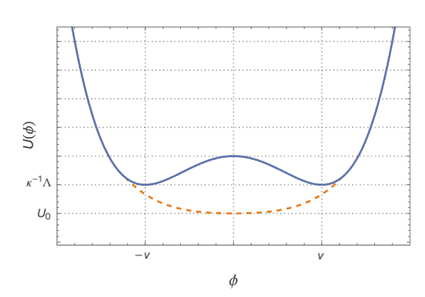
Figure 1: Schematic representation of the bare potential $U(\phi)$ (blue line) and the effective potential $U_{eff}(\phi)$ obtained from tunnelling between the vacua (orange dashed line). $U_{0}$ is given by eq.(3), from which we can see that the effective potential curve reaches a lower value for a smaller volume. In this way the finite volume effects act as a negative contribution to the energy density, and can violate the NEC during a period of contraction.

Using a semi-classical approximation for the partition function, which is dominated by a dilute gas of instantons and anti-instantons, it was shown in [29, 16] that the resulting effective theory is such that:

1. the true vacuum is symmetric and occurs at $\phi=0$, consistently with convexity of the effective potential when several saddle points are taken into account [30, 31, 32, 33, 34, 35, 36, 37, 38, 39, 40];

2. the corresponding effective action is not extensive (it is not proportional to the volume), but has a non-trivial volume dependence;

3. the resulting ground state fluid violates the NEC.

The above features arise from non-perturbative properties of the partition function, since a convex effective potential cannot be obtained from a bare double-well potential with perturbative quantum corrections only.

The (anti-)instantons considered in [29, 16] depend only on the Euclidean time, and the tunnelling process is similar to the one described in Quantum Mechanics, where tunnelling of a particle in a double-well potential leads to a true ground state energy which is lower than the ground state energy in both individual degenerate wells [41] .

Following the same approximation for the partition function, but in a flat and isotropic Friedmann-Lemaitre-Robertson-Walker universe (FLRW), it was shown in [14] that the above mechanism dynamically generates a cosmic bounce, which is followed by an asymptotic de Sitter phase where tunnelling is suppressed exponentially. In this context, “finite volume” is provided by a unit cell in the form of a 3-torus of volume $V_{cell}$. Some recent works in cosmology have considered the evidence for a closed universe, see for example [44, 45]. However, since we do not see any periodicity in our observable universe, any closed volume must be larger than its current size, so any finite volume effects will now be negligible. The physical size of the closed universe can of course be much smaller far in the past, when our comoving volume was smaller, and thus finite volume effects could have played a role in the early universe.

In the isotropic case of [14], tunnelling between the minima of the double-well potential

$$U(\phi)=\kappa^{-1}\Lambda_{b}+\frac{\lambda_{b}}{24}(\phi^{2}-v_{b}^{2})^{2}~{},$$ (1)

leads to the convex effective potential

$$U_{eff}(\phi)=U_{0}+\frac{1}{2}M^{2}\phi^{2}+{\cal O}(\phi^{4})$$ (2)

where

$$U_{0} = \kappa^{-1}\Lambda\left(1-r\frac{e^{-\alpha_{iso}^{3}}}{\alpha_{iso}^{3/2}}\right)$$ (3)

$$M^{2} = \frac{\lambda v^{2}}{3}\left(1-\frac{27\lambda}{32\pi^{2}}\right)>0~{}.$$

In the above expressions, $\lambda_{b}$, $\Lambda_{b}$ and $v_{b}$ have to be understood as the bare parameters, while $\Lambda$, $\lambda$ and $v$ are the renormalised parameters . Also, $\kappa=8\pi G$ and we have defined

$$r=\frac{\lambda\kappa v^{4}}{3\sqrt{3\pi}~{}\Lambda}~{}~{}~{}~{},~{}~{}~{}~{}\alpha_{iso}^{3}\equiv a^{3}\Sigma~{},$$ (4)

where $\Sigma$ is the action of one instanton relating the bare vacua and $a$ is the FLRW scale factor (we consider $\hbar=c=1)$. The potential is illustrated in Fig. 1.

Both $r$ and $\Sigma$ depend on the field parameters, but $\Sigma$ is also proportional to the volume $V_{cell}$ of the fundamental spatial cell, which therefore needs to be finite for the tunnelling probability $\propto\exp(-\alpha_{iso}^{3})$ to be finite - that is, one requires a closed universe.

The present study extends the work of [14] to the anisotropic case, and considers the impact of other components being present. In this work, an adiabatic approximation is assumed, where the tunnelling rate is large compared to the expansion rate, which allows the use of equilibrium QFT. This approximation is very good in the vicinity of the bounce, which is the regime on which we focus.

Finally, we comment here on the stability of our solution against small fluctuations of the spatial curvature ${}^{(3)}R\ll v^{2}$. For $\xi=0$, the bare potential is not modified and no change would occur in our results. For $\xi\neq 0$ the presence of a small non-vanishing curvature would slightly shift the position of the true vacuum, which would imply a redefinition of the cosmological constant, without changing the overall picture. It is only for large spatial curvature fluctuations $v^{2}\lesssim~{}^{(3)}R$ that our model would break down: the vacua of the bare potential would not be degenerate anymore, such that we would have to take into account the formation of bubbles of true vacuum inside the false vacuum.

III Background II: Homogeneous anisotropic universe description

We review here features of the homogeneous but anisotropic universe relevant to our study, and in particular discuss how the anisotropy can be treated as an additional matter component in the Friedmann equations, assuming an appropriate equation of state. Starting with the anisotropic Bianchi-I metric

$$\text{d}s^{2}=-\text{d}t^{2}+a^{2}_{1}\,\text{d}x^{2}+a^{2}_{2}\,\text{d}y^{2}+a^{2}_{3}\,\text{d}z^{2}~{},$$ (5)

the Friedmann equations read ($i,j=1,2,3$)

$$H_{1}H_{2}+H_{1}H_{3}+H_{2}H_{3} = +\kappa\rho~{},$$ (6)

$$(\mbox{for}~{}i\neq j)~{}~{}~{}~{}H_{i}H_{j}+\frac{\ddot{a}_{i}}{a_{i}}+\frac{\ddot{a}_{j}}{a_{j}} = -\kappa p~{},$$ (7)

where $H_{i}=\dot{a}_{i}/a_{i}$ and as above $\kappa=8\pi G$. Following [46, 47] we note that eq.(6) can be written

$$H^{2}=\frac{\kappa}{3}\rho+\sigma^{2}~{},$$ (8)

where the averaged Hubble rate $H$ and the anisotropy $\sigma^{2}$ are defined as

$$H := \frac{1}{3}(H_{1}+H_{2}+H_{3})~{},$$ (9)

$$\sigma^{2} := \frac{1}{18}\Big{[}(H_{1}-H_{2})^{2}+(H_{2}-H_{3})^{2}+(H_{1}-H_{3})^{2}\Big{]}~{}.$$

Equation (8) shows that $3\kappa^{-1}\sigma^{2}$ can be interpreted as an energy density arising from anisotropy. Similarly, the trace of Friedmann equations can be written

$$\dot{H}+H^{2}=-\frac{\kappa}{6}(\rho+3p)-2\sigma^{2}~{},$$ (10)

such that $3\kappa^{-1}\sigma^{2}$ can also be interpreted as a pressure arising from anisotropy. Anisotropy therefore plays a role similar to a homogeneous perfect fluid with equation of state $w=p/\rho=1$, and we expect that the corresponding energy density scales as $a^{-3(1+w)}=a^{-6}$, where $a=(a_{1}a_{2}a_{3})^{1/3}$ is the average scale factor. This is consistent with Eqs. (7) from which one can show that

$$\dot{H}_{i}-\dot{H}_{j}=-3H(H_{i}-H_{j})~{},$$ (11)

which implies $(H_{i}-H_{j})\propto a^{-3}$ and thus $\sigma^{2}\propto a^{-6}$.

Finally we note that, if a bounce occurs, then at this bounce $H=0$ and $\dot{H}>0$, such that the matter contribution should satisfy at the bounce

$$\rho = -\frac{3}{\kappa}\sigma^{2}\leq 0$$ (12)

$$\rho+3p = -\frac{6}{\kappa}\left(\dot{H}+2\sigma^{2}\right)\leq 0~{},$$

as in the isotropic case.

IV Anisotropic quantum fluid description

As discussed above, in the isotropic case ($a_{1}=a_{2}=a_{3}\equiv a$) and from the effective potential (2), the action for the true ground state $\phi=0$ is

$$S_{eff}^{isotropic}=\int\text{d}^{4}x\sqrt{-g}~{}\kappa^{-1}\Lambda\left(1-r~{}\frac{e^{-\alpha_{iso}^{3}}}{\alpha_{iso}^{3/2}}\right)~{}.$$ (13)

In the anisotropic case (5), the only change to the instanton action $\Sigma$ is via the volume $a^{3}V_{cell}\to a_{1}a_{2}a_{3}V_{cell}$, such that the action (13) must be modified as

$$S_{eff}=\int\text{d}^{4}x\sqrt{-g}~{}\kappa^{-1}\Lambda\left(1-r~{}\frac{e^{-\alpha_{1}\alpha_{2}\alpha_{3}}}{\sqrt{\alpha_{1}\alpha_{2}\alpha_{3}}}\right)~{},$$ (14)

where $\alpha_{i}\equiv a_{i}\Sigma^{1/3}$. The stress-energy tensor can be decomposed as

$$T_{\mu\nu}\equiv\frac{2}{\sqrt{-g}}\frac{\delta S_{eff}}{\delta g^{\mu\nu}}=\textrm{diag}(\rho,a_{1}^{2}\,p,a_{2}^{2}\,p,a_{3}^{2}\,p)~{},$$ (15)

and leads to the dimensionless energy density and pressure

$$\tilde{\rho} \equiv \frac{\kappa\rho}{\Lambda}=1-r~{}\frac{e^{-\alpha^{3}}}{\alpha^{3/2}}~{},$$ (16)

$$\tilde{p} \equiv \frac{\kappa p}{\Lambda}=-1+r~{}\left(\frac{1}{2\alpha^{3/2}}-\alpha^{3/2}\right)e^{-\alpha^{3}}~{},$$

where the average scale factor $\alpha$ is defined by

$$\alpha^{3}\equiv a_{1}a_{2}a_{3}\Sigma~{}.$$ (17)

In the previous expressions and from its definition in Eq.(4), $r$ describes the quantum field – it is completely determined once we specify its mass, vacuum energy and self interaction strength (via the parameters $v$, $\Lambda$ and $\lambda$). The pressure and energy density are therefore determined by the combination of field parameters $r$ and the average size of the universe $a\,V_{cell}^{1/3}$.

The Friedmann equations read, in terms of the rescaled quantities, with the rescaled time $\tau\equiv t~{}\sqrt{\Lambda/3}$,

$$\frac{\mathcal{H}_{1}\mathcal{H}_{2}}{3}+\frac{\mathcal{H}_{1}\mathcal{H}_{3}}{3}+\frac{\mathcal{H}_{2}\mathcal{H}_{3}}{3} = +\tilde{\rho}~{},$$ (18)

$$(\mbox{for}~{}i\neq j)~{}~{}~{}~{}\frac{\mathcal{H}_{i}\mathcal{H}_{j}}{3}+\frac{\alpha_{i}^{\prime\prime}}{3\alpha_{i}}+\frac{\alpha_{j}^{\prime\prime}}{3\alpha_{j}} = -\tilde{p}~{},$$ (19)

where a prime refers to the derivative with respect to $\tau$. We can then define the rescaled average Hubble rate $\mathcal{H}$ and anisotropy $\tilde{\sigma}^{2}$

$$\mathcal{H} := \frac{1}{3}(\mathcal{H}_{1}+\mathcal{H}_{2}+\mathcal{H}_{3})~{},$$ (20)

$$\tilde{\sigma}^{2} := \frac{1}{18}\Big{[}(\mathcal{H}_{1}-\mathcal{H}_{2})^{2}+(\mathcal{H}_{2}-\mathcal{H}_{3})^{2}+(\mathcal{H}_{1}-\mathcal{H}_{3})^{2}\Big{]}~{},$$

so that eq.(18) can be simply written as

$$\mathcal{H}^{2}=\tilde{\rho}+\tilde{\sigma}^{2}~{}.$$ (21)

We can see from eq. (12) that $\tilde{\rho}<0$ and $\tilde{\rho}+3\tilde{p}<0$, in order to balance out the anisotropy contribution in the vicinity of the average bounce, defined by $\mathcal{H}=0$ and $\mathcal{H}^{\prime}>0$. In what follows, we will study under which conditions the cosmological bounce can be induced.

V Critical solutions

As discussed in the previous section, in a universe with significant anisotropy, an additional contribution to the energy density and the pressure of the spacetime exists. Starting from some initial condition, several scenarios are possible given the different scalings in $\alpha$. The NEC violation from tunnelling does not necessarily win over the anisotropy during the collapse (even where it is initially larger) a bounce requires not only that both contributions cancel each other such that $\mathcal{H}=0$, but also that at this point of equality, the pressure satisfies the necessary condition for the universe to bounce (i.e., $\mathcal{H}^{\prime}>0$). For this latter condition to be true, the size of the universe at this point must be sufficiently small (relative to the field parameters) for finite volume effects to be significant, but not too small to avoid a collapse. In this section we derive the specific requirements, and comment on the resulting phenomenology.

V.1 Critical point

The critical solution of the Friedmann equations for which a bounce occurs $(\rho_{c},p_{c},\alpha_{c},\tilde{\sigma}_{c}^{2})$ can be found by imposing the condition $\mathcal{H}=\mathcal{H}^{\prime}=0$. This critical point is unstable: a value of $\alpha$ that is slightly larger than $\alpha_{c}$ leads to a bounce (the NEC violation $\propto\alpha^{-3/2}$ dominates) and a value which is slightly smaller leads to a collapse (the anisotropy $\propto\alpha^{-6}$ dominates).

From these conditions, the energy density and the pressure at the critical point satisfy

$$\tilde{p}_{c}=\tilde{\rho}_{c}=-\tilde{\sigma}^{2}_{c}~{}.$$ (22)

Also, from Eqs. (16), we find that the averaged scale factor $\alpha_{c}$ is given by the implicit algebraic equation

$$4\alpha_{c}^{3/2}+re^{-\alpha_{c}^{3}}(-3+2\alpha^{3}_{c})=0~{},$$ (23)

and the anisotropy can be expressed as

$$\tilde{\sigma}^{2}_{c}=\frac{1+2\alpha^{3}_{c}}{3-2\alpha^{3}_{c}}~{}.$$ (24)

We can see from Eq. (23) that necessarily $\alpha_{c}^{3}<3/2$, and one can identify the two regimes

$$\alpha_{c} \to (3/2)^{1/3}~{}~{}~{}~{}\mbox{for}~{}~{}r\gg 1$$ (25)

$$\alpha_{c} \sim \left(\frac{3r}{4}\right)^{2/3}~{}~{}~{}~{}\mbox{for}~{}~{}r\ll 1~{}.$$

One can understand the role of $\alpha_{c}$ from the point of view of the pressure. Assume that there is a time $\tau_{1}$ where $\mathcal{H}(\tau_{1})=0$:

• A bounce requires the condition $\mathcal{H}^{\prime}(\tau_{1})>0$, and thus $|\tilde{p}(\tau_{1})|>|\tilde{\rho}(\tau_{1})|$, such that

  $$4\alpha^{3/2}(\tau_{1})+re^{-\alpha^{3}(\tau_{1})}[-3+2\alpha^{3}(\tau_{1})]>0~{},$$ (26)

  which leads to $\alpha(\tau_{1})>\alpha_{c}$;
  

• A collapse follows in the situation where $\mathcal{H}^{\prime}(\tau_{1})<0$, and thus $|\tilde{p}(\tau_{1})|<|\tilde{\rho}(\tau_{1})|$, such that

  $$4\alpha^{3/2}(\tau_{1})+re^{-\alpha^{3}(\tau_{1})}[-3+2\alpha^{3}(\tau_{1})]<0~{},$$ (27)

  which leads to $\alpha(\tau_{1})<\alpha_{c}$.

V.2 Comparison with the isotropic case

One can also infer a maximum value for the rescaled scale factor $\alpha_{iso}$ at the bounce, which happens when the anisotropy (and any other components if there are) are negligible and the quantum field completely dominates. We then have from Eq. (16)

$$\alpha_{iso}^{3/2}=r~{}e^{-\alpha_{iso}^{3}}~{},$$ (28)

which leads to the two regimes

$$\alpha_{iso} \sim (\ln r)^{1/3}~{}~{}~{}~{}\mbox{for}~{}~{}~{}~{}r\gg 1$$ (29)

$$\alpha_{iso} \sim r^{2/3}~{}~{}~{}~{}\mbox{for}~{}~{}~{}~{}r\ll 1~{},$$ (30)

and we note that $\alpha_{iso}$ is not bounded when $r\to\infty$. We sketch $\alpha_{c}$ and $\alpha_{iso}$ on Fig.2, where the region between the two curves represents the possible range of values of the rescaled scale factor at which a bounce can occur for a particular quantum field (as parametrised by $r$).

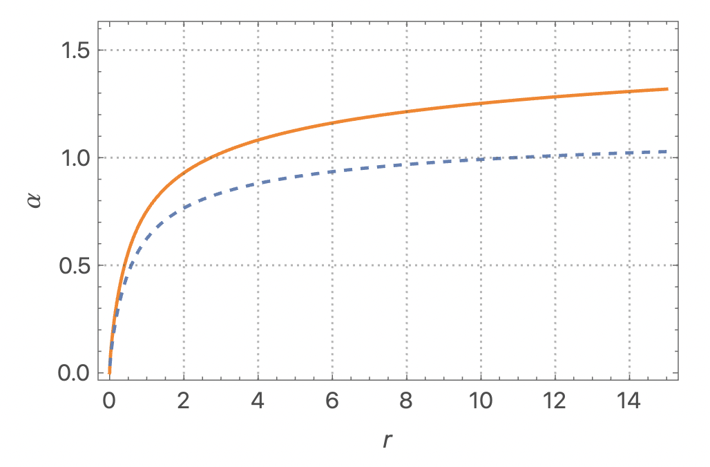
Figure 2: A plot of the rescaled average scale factor at the bounce $\alpha=a\Sigma^{1/3}$ (which is related to the size of the closed universe) versus $r$ (which is determined by the properties of the field). We plot the maximum $\alpha_{iso}$ (orange line) and minimum $\alpha_{c}$ (dashed blue line) values, as a function of $r$. Although $\alpha_{c}$ asymptotically tends to $(3/2)^{1/3}$, $\alpha_{iso}$ is not bounded and goes to infinity when $r\to\infty$.

V.3 Size of the Universe at the bounce

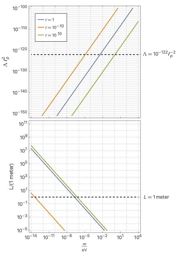
Figure 3: These plots illustrate consistent values of the field parameters and the size $L_{b}$ of the closed universe at the bounce for different values of the field parameter $r$. The upper plot shows the relation between $\Lambda$ and $m$. The lower plot shows the relation between the maximum value for $L_{b}$ and $m$ (the minimum of $L_{b}$ has very similar values and is not represented for the sake of clarity - thus the range of possible values between the limits in Fig. 2 all lie close to the lines in this plot). We note that the function $L_{b}(m)$ is almost independent of $r$ for $r\gg 1$, whereas it changes significantly for $r\ll 1$.

From the previous results one can put bounds on the typical physical size of the universe at the bounce, for a given field. The instanton action is of the order [16]

$$\Sigma\sim\frac{m^{3}}{\lambda}V_{cell}~{},$$ (31)

where $m=v\sqrt{\lambda/3}$. The physical length $L$ is given by $L=a(t)V_{cell}^{1/3}$ and its value at the bounce then satisfies

$$\lambda^{1/3}~{}\frac{\alpha_{c}}{m}~{}\lesssim~{}L_{b}~{}\lesssim~{}\lambda^{1/3}~{}\frac{\alpha_{iso}}{m}~{}.$$ (32)

To get a feel for the phenomenological consequences of the model, we can relate the field quantities $m$ and $\Lambda$ with the size of the closed universe at the bounce $L_{b}$, parameterised by the ratio $r$. For simplicity we assume here that $\lambda^{1/3}$ is of order 1 .

The current size of the visible universe is $\sim 10^{26}$ meters, and we do not see any evidence of periodicity in it [50]. Any bounce must have happened before the electroweak phase transition, at which point the size of our observable universe was about $10^{11}$ meters. This therefore imposes a minimum on the size of the closed universe at the bounce - any smaller and we would see evidence for periodicity now. However, a bounce could also have occurred much earlier than this and so the universe could have been smaller. If instead we take the bounce to occur at the era of grand unification, the size of the closed universe would be of order $1$ meter or larger.

As can be seen from Fig.3, for $r=1$, if the bounce occurred when $L\sim 1$ m, the scalar field would need a bare mass of $\sim 10^{-7}$ eV and a vacuum energy $\Lambda$ of order $10^{-140}~{}\ell_{p}^{-2}$, therefore much smaller than the current cosmological constant. The plot illustrates how the values change for different values of $r$, but in general one requires a larger mass to be consistent with a smaller $L$, and small values for the vacuum energy are required.

VI Numerical solutions

In this section we numerically integrate the Friedmann equations (18), both in the bouncing case (where NEC violation dominates) and in the collapsing case (where the anisotropy dominates), to illustrate the possible outcomes.

We choose the initial anisotropy $\tilde{\sigma}^{2}(\tau_{0})$ as one of the parameters. For simplicity, we will consider $\alpha_{2}(\tau_{0})=\alpha(\tau_{0})$ and $\mathcal{H}_{2}(\tau_{0})=\mathcal{H}(\tau_{0})$. Hence from (20) we find for all times

$$\mathcal{H}_{1} = \mathcal{H}\pm\sqrt{3\tilde{\sigma}^{2}}~{},$$ (33)

$$\mathcal{H}_{2} = \mathcal{H}~{},$$ (34)

$$\mathcal{H}_{3} = \mathcal{H}\mp\sqrt{3\tilde{\sigma}^{2}}~{}.$$ (35)

The initial value of $\mathcal{H}$ can then be determined by equations (21) and (16), namely

$$\mathcal{H}^{2}(\tau_{0})=\tilde{\sigma}^{2}(\tau_{0})+1-r\frac{e^{-\alpha^{3}(\tau_{0})}}{\alpha^{3/2}(\tau_{0})}~{}.$$ (36)

We take the negative root $\mathcal{H}(\tau_{0})<0$ since we want to start from a contracting phase. As a consequence, the initial Hubble rates are entirely determined by $\tilde{\sigma}^{2}(\tau_{0})$, and for the numerical analysis the quantities we fix are $\tilde{\sigma}^{2}(\tau_{0})$, $\alpha(\tau_{0})$ and $r$.

We take $r\leq e$, so that we are before the point of equality in the energy densities in the anisotropy and the quantum field. For these values of $r$, we choose the initial average scale factor such that $\alpha^{3}(\tau_{0})=\alpha_{1}(\tau_{0})\alpha_{2}(\tau_{0})\alpha_{3}(\tau_{0})=1$. This allows the bounce to happen soon after the initial time, compared to the typical time scale of the whole process. A larger initial scale factor would shift the time when the bounce occurs.

Fig.4 shows an example of a bouncing solution. We include the time evolution of the scale factors $\alpha_{i}$, and Hubble rates $\mathcal{H}_{i}$, the anisotropy $\tilde{\sigma}^{2}$, and the energy density $\tilde{\rho}$. We choose $r=2$, and initial conditions at $\tau_{0}=0$ $\alpha_{i}(\tau_{0})=\{2/3,1,3/2\}$, and $\tilde{\sigma}^{2}(\tau_{0})=0.05$.

Fig.5 shows an example of a case where the bounce is not reached, due to the anisotropy dominating, but that is close to the critical case. The initial conditions are $r=2$, $\alpha_{i}(\tau_{0})=\{2/3,1,3/2\}$ and $\tilde{\sigma}^{2}(\tau_{0})=0.18247$.

VII Discussion

In this work we have studied the possibility of a cosmic bounce occurring in a universe in which there is a significant (but not dominant) anisotropy, in addition to the presence of a scalar field which is subject to finite volume effects in a closed universe. We have shown that criteria for the success of the bounce can be stated in terms of the size of the closed universe at the point at which the net energy density is zero, and have studied the properties of the quantum field (mass and vacuum energy) that permit a bounce of a size consistent with our own cosmological history.

At the point of zero net energy density, the size of the universe must be roughly comparable to the Compton wavelength of the field for its pressure to be sufficient to turn around the collapse, so values smaller than $\sim 10^{-5}$ eV are needed for the mass. We also find that the vacuum energy of the field must be extremely small, even in comparison to the current day cosmological constant. After the bounce, the universe transitions to expansion and the contribution of the quantum field to the energy density reduces to its vacuum energy, with finite volume effects completely suppressed. The fact that this vacuum energy is smaller than the current value is therefore consistent with what we observe (it could be a small contribution to its value), but the smallness of the value seems to require some further explanation – although this is of course true of the cosmological constant itself.

Examples of further consequences of tunnelling effects in finite volume are as follows: One could involve an out-of-equilibrium QFT description of tunnelling in the background of a time-varying metric, which would allow a more accurate study away from the bounce. Then, the inclusion of the Casimir effect due to the finite volume $V_{cell}$ could give rise to new effects, with possible cosmological relevance. Also, the effect of spatial curvature should be included, in the situation where the space fundamental cell is a 3-sphere instead of a 3-torus. These studies are left for future works.

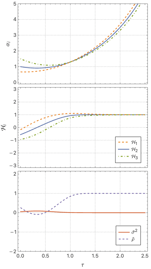
Figure 4: Bouncing case: In the two upper panels we show the time evolution of the rescaled scale factors $\alpha_{i}$ and the rescaled Hubble rates $\mathcal{H}_{i}$ with the initial conditions given in the main text. The lower panel shows the time evolution of the anisotropy $\tilde{\sigma}^{2}$ and energy density $\tilde{\rho}$.

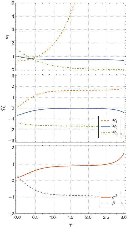
Figure 5: Near critical no-bounce case: In the two upper panels we show the time evolution of the rescaled scale factors $\alpha_{i}$ and the rescaled Hubble rates $\mathcal{H}_{i}$ with the initial conditions given in the main text. The lower panel shows the time evolution of the anisotropy $\tilde{\sigma}^{2}$ and energy density $\tilde{\rho}$. The initial conditions are close to the critical point and for a time the value of the rescaled average Hubble rate $\mathcal{H}$ remains near zero. However, eventually the average scale factor grows, leading to another collapsing phase in which the anisotropy diverges.

References

- Akrami et al. [2020] Y. Akrami et al. (Planck), Planck 2018 results. X. Constraints on inflation, Astron. Astrophys. 641, A10 (2020), arXiv:1807.06211 [astro-ph.CO] .
- Guth [1981] A. H. Guth, The Inflationary Universe: A Possible Solution to the Horizon and Flatness Problems, Phys. Rev. D 23, 347 (1981).
- Linde [1982] A. D. Linde, A New Inflationary Universe Scenario: A Possible Solution of the Horizon, Flatness, Homogeneity, Isotropy and Primordial Monopole Problems, Phys. Lett. B 108, 389 (1982).
- Albrecht and Steinhardt [1982] A. Albrecht and P. J. Steinhardt, Cosmology for Grand Unified Theories with Radiatively Induced Symmetry Breaking, Phys. Rev. Lett. 48, 1220 (1982).
- Brandenberger [2016] R. Brandenberger, Initial conditions for inflation — A short review, Int. J. Mod. Phys. D 26, 1740002 (2016), arXiv:1601.01918 [hep-th] .
- Hawking and Penrose [1970] S. W. Hawking and R. Penrose, The Singularities of gravitational collapse and cosmology, Proc. Roy. Soc. Lond. A 314, 529 (1970).
- Borde and Vilenkin [1994] A. Borde and A. Vilenkin, Eternal inflation and the initial singularity, Phys. Rev. Lett. 72, 3305 (1994), arXiv:gr-qc/9312022 .
- Rubakov [2014] V. A. Rubakov, The Null Energy Condition and its violation, Phys. Usp. 57, 128 (2014), arXiv:1401.4024 [hep-th] .
- Kontou and Sanders [2020] E.-A. Kontou and K. Sanders, Energy conditions in general relativity and quantum field theory, Class. Quant. Grav. 37, 193001 (2020), arXiv:2003.01815 [gr-qc] .
- Khoury et al. [2001] J. Khoury, B. A. Ovrut, P. J. Steinhardt, and N. Turok, The Ekpyrotic universe: Colliding branes and the origin of the hot big bang, Phys. Rev. D 64, 123522 (2001), arXiv:hep-th/0103239 .
- Khoury et al. [2002] J. Khoury, B. A. Ovrut, N. Seiberg, P. J. Steinhardt, and N. Turok, From big crunch to big bang, Phys. Rev. D 65, 086007 (2002), arXiv:hep-th/0108187 .
- Steinhardt and Turok [2002] P. J. Steinhardt and N. Turok, Cosmic evolution in a cyclic universe, Phys. Rev. D 65, 126003 (2002), arXiv:hep-th/0111098 .
- Ijjas and Steinhardt [2018] A. Ijjas and P. J. Steinhardt, Bouncing Cosmology made simple, Class. Quant. Grav. 35, 135004 (2018), arXiv:1803.01961 [astro-ph.CO] .
- Alexandre and Pla [2023] J. Alexandre and S. Pla, Cosmic bounce and phantom-like equation of state from tunnelling, JHEP 05, 145, arXiv:2301.08652 [hep-th] .
- Bordag et al. [2001] M. Bordag, U. Mohideen, and V. M. Mostepanenko, New developments in the Casimir effect, Phys. Rept. 353, 1 (2001), arXiv:quant-ph/0106045 .
- Alexandre and Backhouse [2023] J. Alexandre and D. Backhouse, Null energy condition violation: Tunneling versus the Casimir effect, Phys. Rev. D 107, 085022 (2023), arXiv:2301.02455 [hep-th] .
- Trautman [1973] A. Trautman, Spin and torsion may avert gravitational singularities, Nature 242, 7 (1973).
- Alexander and Biswas [2009] S. Alexander and T. Biswas, The Cosmological BCS mechanism and the Big Bang Singularity, Phys. Rev. D 80, 023501 (2009), arXiv:0807.4468 [hep-th] .
- Magueijo et al. [2013] J. a. Magueijo, T. G. Zlosnik, and T. W. B. Kibble, Cosmology with a spin, Phys. Rev. D 87, 063504 (2013), arXiv:1212.0585 [astro-ph.CO] .
- Tukhashvili and Steinhardt [2023] G. Tukhashvili and P. J. Steinhardt, Cosmological Bounces Induced by a Fermion Condensate, Phys. Rev. Lett. 131, 091001 (2023), arXiv:2307.16098 [gr-qc] .
- Erickson et al. [2004] J. K. Erickson, D. H. Wesley, P. J. Steinhardt, and N. Turok, Kasner and mixmaster behavior in universes with equation of state w = 1, Phys. Rev. D 69, 063514 (2004), arXiv:hep-th/0312009 .
- Hu [2021] B.-L. Hu, Weyl Curvature Hypothesis in Light of Quantum Backreaction at Cosmological Singularities or Bounces, Universe 7, 424 (2021), arXiv:2110.01104 [gr-qc] .
- Halliwell and Louko [1989] J. J. Halliwell and J. Louko, Steepest Descent Contours in the Path Integral Approach to Quantum Cosmology. 1. The De Sitter Minisuperspace Model, Phys. Rev. D 39, 2206 (1989).
- Feldbrugge et al. [2017] J. Feldbrugge, J.-L. Lehners, and N. Turok, Lorentzian Quantum Cosmology, Phys. Rev. D 95, 103508 (2017), arXiv:1703.02076 [hep-th] .
- Di Tucci et al. [2019] A. Di Tucci, J. Feldbrugge, J.-L. Lehners, and N. Turok, Quantum Incompleteness of Inflation, Phys. Rev. D 100, 063517 (2019), arXiv:1906.09007 [hep-th] .
- Rajeev et al. [2022] K. Rajeev, V. Mondal, and S. Chakraborty, Bouncing with shear: implications from quantum cosmology, JCAP 01 (01), 008, arXiv:2109.08696 [gr-qc] .
- Barca et al. [2021] G. Barca, E. Giovannetti, and G. Montani, An Overview on the Nature of the Bounce in LQC and PQM, Universe 7, 327 (2021), arXiv:2109.08645 [gr-qc] .
- Barca et al. [2022] G. Barca, E. Giovannetti, and G. Montani, Comparison of the semiclassical and quantum dynamics of the Bianchi I cosmology in the polymer and GUP extended paradigms, Int. J. Geom. Meth. Mod. Phys. 19, 2250097 (2022), arXiv:2112.08905 [gr-qc] .
- Alexandre and Polonyi [2022] J. Alexandre and J. Polonyi, Symmetry restoration, tunneling, and the null energy condition, Phys. Rev. D 106, 065008 (2022), arXiv:2205.00768 [hep-th] .
- Symanzik [1970] K. Symanzik, Renormalizable models with simple symmetry breaking. 1. Symmetry breaking by a source term, Commun. Math. Phys. 16, 48 (1970).
- Coleman et al. [1974] S. R. Coleman, R. Jackiw, and H. D. Politzer, Spontaneous Symmetry Breaking in the O(N) Model for Large N*, Phys. Rev. D 10, 2491 (1974).
- Iliopoulos et al. [1975] J. Iliopoulos, C. Itzykson, and A. Martin, Functional Methods and Perturbation Theory, Rev. Mod. Phys. 47, 165 (1975).
- Fujimoto et al. [1983] Y. Fujimoto, L. O’Raifeartaigh, and G. Parravicini, Effective Potential for Nonconvex Potentials, Nucl. Phys. B 212, 268 (1983).
- Haymaker and Perez-Mercader [1983] R. W. Haymaker and J. Perez-Mercader, Convexity of the Effective Potential, Phys. Rev. D 27, 1948 (1983).
- Bender and Cooper [1983] C. M. Bender and F. Cooper, Failure of the Naive Loop Expansion for the Effective Potential in Field Theory When There Is ’Broken Symmetry’, Nucl. Phys. B 224, 403 (1983).
- Hindmarsh and Johnston [1986] M. Hindmarsh and D. Johnston, Convexity of the Effective Potential, J. Phys. A 19, 141 (1986).
- Alexandre and Tsapalis [2013] J. Alexandre and A. Tsapalis, Maxwell Construction for Scalar Field Theories with Spontaneous Symmetry Breaking, Phys. Rev. D 87, 025028 (2013), arXiv:1211.0921 [hep-th] .
- Plascencia and Tamarit [2016] A. D. Plascencia and C. Tamarit, Convexity, gauge-dependence and tunneling rates, JHEP 10, 099, arXiv:1510.07613 [hep-ph] .
- Millington and Saffin [2019] P. Millington and P. M. Saffin, Visualising quantum effective action calculations in zero dimensions, J. Phys. A 52, 405401 (2019), arXiv:1905.09674 [hep-th] .
- Alexandre and Backhouse [2022] J. Alexandre and D. Backhouse, One-loop tunneling-induced energetics, Phys. Rev. D 105, 105018 (2022), arXiv:2203.12543 [hep-th] .
- Kleinert [2004] H. Kleinert, Path Integrals in Quantum Mechanics, Statistics, Polymer Physics, and Financial Markets (World Scientific, Singapore, 2004).
- Coleman [1977] S. R. Coleman, The Fate of the False Vacuum. 1. Semiclassical Theory, Phys. Rev. D 15, 2929 (1977), [Erratum: Phys.Rev.D 16, 1248 (1977)].
- Callan and Coleman [1977] C. G. Callan, Jr. and S. R. Coleman, The Fate of the False Vacuum. 2. First Quantum Corrections, Phys. Rev. D 16, 1762 (1977).
- Di Valentino et al. [2019] E. Di Valentino, A. Melchiorri, and J. Silk, Planck evidence for a closed Universe and a possible crisis for cosmology, Nature Astron. 4, 196 (2019), arXiv:1911.02087 [astro-ph.CO] .
- Handley [2021] W. Handley, Curvature tension: Evidence for a closed universe, ”Phys. Rev. D” 103, L041301 (2021), arXiv:1908.09139 [astro-ph.CO] .
- Barrow [1995] J. D. Barrow, Why the universe is not anisotropic, Phys. Rev. D 51, 3113 (1995).
- Ellis and van Elst [1999] G. F. R. Ellis and H. van Elst, Cosmological models: Cargese lectures 1998, NATO Sci. Ser. C 541, 1 (1999), arXiv:gr-qc/9812046 .
- Marsh [2016] D. J. E. Marsh, Axion Cosmology, Phys. Rept. 643, 1 (2016), arXiv:1510.07633 [astro-ph.CO] .
- Mavromatos and Sarkar [2023] N. E. Mavromatos and S. Sarkar, Axion effective potentials induced by heavy sterile fermions, Eur. Phys. J. C 83, 866 (2023), arXiv:2306.02122 [hep-th] .
- Baumann [2022] D. Baumann, Cosmology (Cambridge University Press, 2022).