Decomposition Ascribed Synergistic Learning for Unified Image Restoration

Abstract

Learning to restore multiple image degradations within a single model is quite beneficial for real-world applications. Nevertheless, existing works typically concentrate on regarding each degradation independently, while their relationship has been less exploited to ensure the synergistic learning. To this end, we revisit the diverse degradations through the lens of singular value decomposition, with the observation that the decomposed singular vectors and singular values naturally undertake the different types of degradation information, dividing various restoration tasks into two groups, i.e., singular vector dominated and singular value dominated. The above analysis renders a more unified perspective to ascribe the diverse degradations, compared to previous task-level independent learning. The dedicated optimization of degraded singular vectors and singular values inherently utilizes the potential relationship among diverse restoration tasks, attributing to the Decomposition Ascribed Synergistic Learning (DASL). Specifically, DASL comprises two effective operators, namely, Singular VEctor Operator (SVEO) and Singular VAlue Operator (SVAO), to favor the decomposed optimization, which can be lightly integrated into existing convolutional image restoration backbone. Moreover, the congruous decomposition loss has been devised for auxiliary. Extensive experiments on blended five image restoration tasks demonstrate the effectiveness of our method, including image deraining, image dehazing, image denoising, image deblurring, and low-light image enhancement.

I Introduction

Image restoration aims to recover the latent clean images from their degraded observations, and has been widely applied to a series of real-world scenarios, such as photo processing, autopilot, and surveillance. Compared to single-degradation removal [104, 41, 35, 36, 2, 44, 37, 105, 1, 18], the recent flourished multi-degradation learning methods have gathered considerable attention, due to their convenient deployment. However, every rose has its thorn. How to ensure the synergy among multiple restoration tasks demands a dedicated investigation, and it is imperative to include their implicit relationship into consideration.

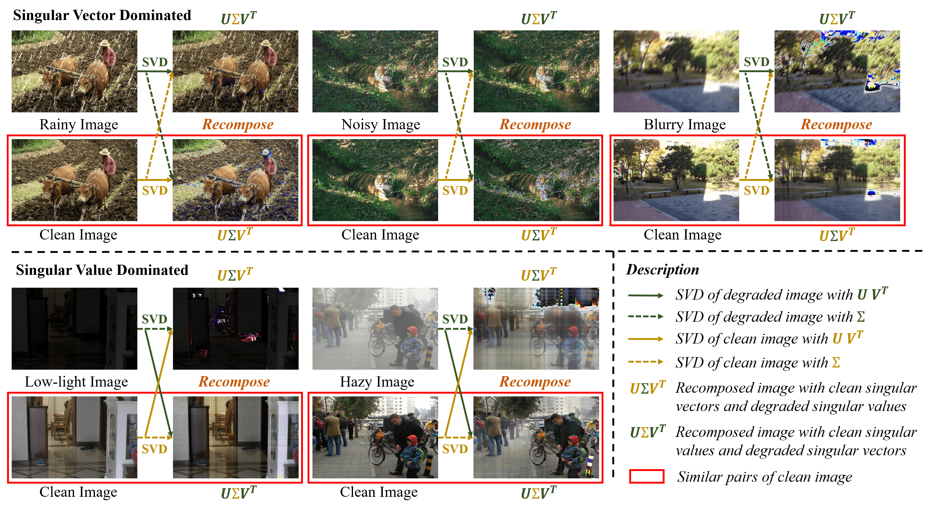
Figure 1: An illustration of the decomposition ascribed analysis on various image restoration tasks through the lens of the singular value decomposition. The decomposed singular vectors and singular values naturally undertake the different types of degradation information, when we recompose the degraded image with portions of the clean counterpart, ascribing various restoration tasks into two groups, i.e., singular vector dominated rain, noise, blur, and singular value dominated low-light, haze. Dedicated to the decomposed optimization of degraded singular vectors and singular values rendering a more unified perspective for synergistic learning, compared to previous task-level independent learning.

Generally, existing multi-degradation learning methods concentrated on regarding each degradation independently. For instance, [15, 22, 16] propose to deal with different restoration tasks through separate subnetworks or distinct transformer queries. [20, 17] propose to distinguish diverse degradation representations via contrastive learning. Remarkably, there are also few attempts devoted to duality degradation removal with synergistic learning. [19] proposes to leverage the blurry and noisy pairs for joint restoration as their inherent complementarity during digital imaging. [82] proposes a unified network with low-light enhancement encoder and deblurring decoder to address hybrid distortion. [21] proposes to quantify the relationship between arbitrary two restoration tasks, and improve the performance of the anchor task with the aid of another task. However, few efforts have been made toward synergistic learning among more restoration tasks, and there is a desperate lack of perspective to revisit the diverse degradations for combing their implicit relationship, which set up the stage for this paper.

To solve the above problem, we propose to revisit diverse degradations through the lens of singular value decomposition, and conduct experiments on five common image restoration tasks, including image deraining, dehazing, denoising, deblurring, and low-light enhancement. As shown in Fig. 1, it can be observed that the decomposed singular vectors and singular values naturally undertake the different types of degradation information, in that the corruptions fade away as we recompose the degraded image with portions of the clean counterpart. Thus, various restoration tasks can be ascribed into two groups, i.e., singular vector dominated degradations and singular value dominated deagradations. The statistic results in Fig. 2 further validate this phenomenon, where the quantified recomposed image quality and the singular distribution discrepancy have been presented. Therefore, the potential relationship emerged among diverse restoration tasks could be inherently utilized through the decomposed optimization of singular vectors and singular values, considering their ascribed common properties and significant discrepancies.

In this way, we decently convert the previous task-level independent learning into more unified singular vectors and singular values learning, and form our method, Decomposition Ascribed Synergistic Learning (DASL). Basically, one straightforward way to implement our idea is to directly perform the decomposition on latent high-dimensional tensors, and conduct the optimization for decomposed singular vectors and singular values, respectively. However, the huge computational overhead is non-negligible. To this end, two effective operators have been developed to favor the decomposed optimization, namely, Singular VEctor Operator (SVEO) and Singular VAlue Operator (SVAO). Specifically, SVEO takes advantage of the fact that the orthogonal matrices multiplication makes no effect on singular values and only impacts singular vectors, which can be realized through simple regularized convolution layer. SVAO resorts to the signal formation homogeneity between Singular Value Decomposition and the Inverse Discrete Fourier Transform, which can both be regarded as a weighted sum on a set of basis. While the decomposed singular values and the transformed fourier coefficients essentially undertake the same role for linear combination. And the respective base components share similar principle, i.e.from outline to details. Therefore, with approximate derivation, the unattainable singular values optimization can be translated to accessible spectrum maps. We show that the fast fourier transform is substantially faster than the singular value decomposition. Furthermore, the congruous singular decomposition loss has been devised for auxiliary. The proposed DASL can be lightly integrated into existing convolutional image restoration backbone for decomposed optimization.

The contributions of this work are summarized below:

• We take a step forward to revisit the diverse degradations through the lens of singular value decomposition, and observe that the decomposed singular vectors and singular values naturally undertake the different types of degradation information, ascribing various restoration tasks into two groups, i.e.singular vector dominated and singular value dominated.

• We propose the Decomposition Ascribed Synergistic Learning (DASL) to dedicate the decomposed optimization of degraded singular vectors and singular values respectively, which inherently utilizes the potential relationship among diverse restoration tasks.

• Two effective operators have been developed to favor the decomposed optimization, along with a congruous decomposition loss, which can be lightly integrated into existing convolutional image restoration backbone. Extensive experiments on five image restoration tasks demonstrate the effectiveness of our method.

II Related work

In this section, we briefly review the recent developments in image restoration and tensor decomposition.

Image Restoration. Image restoration aims to recover the latent clean images from degraded observations, which has been studied for a long term. Traditional image restoration methods typically concentrated on incorporating various natural image priors along with hand-crafted features for specific degradation removal [6, 5, 3]. Recently, learning-based methods have made compelling progress on various image restoration tasks, including image denoising [2, 45, 44], image deraining [42, 104, 41], image deblurring [37, 38, 39], image dehazing [33, 35, 36], and low-light image enhancement [1, 30, 106], etc. Moreover, numerous general image restoration methods have also been proposed. [14, 92, 12] propose a delicate balance between contextual information and spatial details for general image restoration. [25, 26] formulate the image restoration via unfolding strategy to deep into the rationality. [7, 96] proposes to exploit the frequency characteristics to handle diverse degradations. Additionally, various transformer-based methods [13, 27, 28, 29, 23] have also been investigated for image restoration, due to their impressive performance in modeling global dependencies as well as superior adaptability to input content.

Recently, recovering multiple image degradations within a single model has been coming to the fore, as they are more in line with real-world applications. [19] proposes to leverage the short-exposure noisy image and the long-exposure blurry image for joint restoration as their inherent complementarity during digital imaging. [82] proposes a unified network to address low-light image enhancement and image deblurring. Furthermore, numerous all-in-one fashion methods [15, 22, 20, 16, 17] have been proposed to deal with more degradations. However, the majority of them concentrated on the network architecture design as well as the training strategy, and few attempts have been made to explore the synergy among diverse restoration tasks, compared to the duality degradation removal.

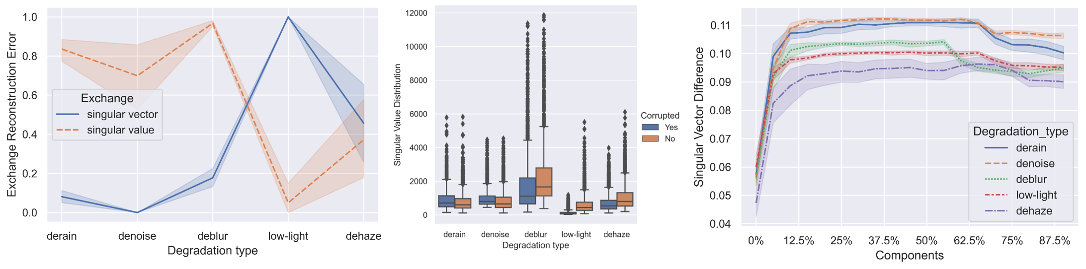
Figure 2: The statistic validation that the decomposed singular vectors and singular values undertake the different types of degradation information. (a) The reconstruction error between the recomposed image and paired clean image on five common image restoration tasks, where the degraded singular vectors or singular values have been exchanged with corresponding clean counterparts. Low error denotes the degradation primarily distributed in the replaced portion of the image. (b) The boxplot comparison of singular value distribution between the degraded image and the corresponding clean image, where the singular value dominated low-light and haze exhibit the extraordinary difference. (c) The singular vector difference on separate orders of the component between the degraded image and clean image, where the singular vector dominated rain, noise, and blur present more disparity. The results are obtained under calculation on 100 images for each restoration task.

Tensor Decomposition. Tensor decomposition has been widely applied to a series of fields, such as model compression [46, 50], neural rendering [47], multi-task learning [49], and reinforcement learning [48]. In terms of image restoration, a large number of decomposition-based methods have been proposed for hyperspectral and multispectral image restoration [52, 51, 53, 54], in that establishing their spatial-spectral correlation with low-rank approximation.

Alternatively, a surge of filter decomposition methods toward networks have also been developed. [55, 56, 57] propose to approximate the original filters with efficient representations to reduce the network parameters and inference time. [49] proposes to reparameterize the convolution operators for multi-task learning. [91] proposes to decompose the backbone network via the singular value decomposition, and only finetune the singular values for few-shot segmentation.

III Method

In this section, we start with introducing the overall framework of our Decomposition Ascribed Synergistic Learning in Sec. III-A, and then elaborate the singular vector operator and singular value operator in Sec. III-B and Sec. III-C, respectively, which forming our core components. The optimization objective is briefly presented in Sec. III-D.

III-A Overview

The intention of the proposed Decomposition Ascribed Synergistic Learning (DASL) is to dedicate the decomposed optimization of degraded singular vectors and singular values respectively, since they naturally undertake the different types of degradation information as observed in Figs. 1 and 2. And the decomposed optimization renders a more unified perspective to revisit diverse degradations for ascribed synergistic learning. Through examining the singular vector dominated degradations which containing rain, noise, blur, and singular value dominated degradations including hazy, low-light, we make the following assumptions: (i) The singular vectors responsible for the content information and spatial details, (ii) The singular values represent the global statistical properties of the image. Therefore, the optimization of the degraded singular vectors could be performed throughout the backbone network. And the optimization for the degraded singular values can be condensed to a few of pivotal positions. Specifically, we substitute half of the convolution layers with SVEO, which are uniformly distributed across the entire network. While the SVAOs are only performed at the bottleneck layers of the backbone network. We ensure the compatibility between the optimized singular values and singular vectors through remaining regular layers, and the proposed DASL can be lightly integrated into existing convolutional image restoration backbone for decomposed optimization.

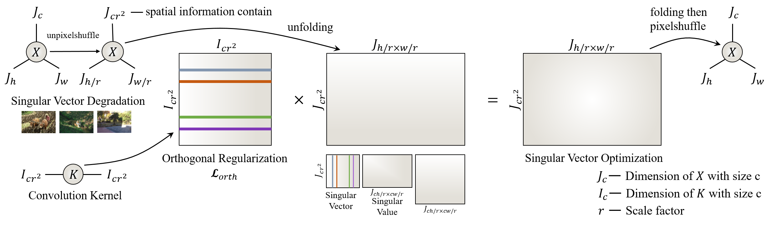
Figure 3: An illustration of the proposed Singular Vector Operator (SVEO), which is dedicated on the optimization of the singular vector dominated degradations, i.e.rain, noise, blur. Theorem 1 supports the feasibility and the orthogonal regularization $\mathcal{L}_{orth}$ refers to Eq. 3.

III-B Singular Vector Operator

The singular vector operator is proposed to optimize the degraded singular vectors of the latent representation, and supposed to be decoupled from the optimization of singular values. Explicitly performing the singular value decomposition on high-dimensional tensors solves this problem naturally with little effort, however, the huge computational overhead is non-negligible. Whether can we modify the singular vectors with less computation burden. The answer is affirmative and lies in the orthogonal matrices multiplication.

Theorem 1.

For an arbitrary matrix $X\in\mathbb{R}^{h\times w}$ and random orthogonal matrices $P\in\mathbb{R}^{h\times h},Q\in\mathbb{R}^{w\times w}$, the products of the $PX$, $XQ$, $PXQ$ have the same singular values with the original matrix $X$.

Proof. According to the definition of Singular Value Decomposition (SVD), we can decompose matrix $X\in\mathbb{R}^{h\times w}$ into $USV^{T}$, where $U\in\mathbb{R}^{h\times h}$ and $V\in\mathbb{R}^{w\times w}$ indicate the orthogonal singular vector matrices, $S\in\mathbb{R}^{h\times w}$ indicates the diagonal singular value matrix. Thus $X^{{}^{\prime}}$=$PXQ$=$PUSV^{T}Q$. Denotes $U^{{}^{\prime}}$=$PU$ and $V^{{}^{\prime}T}$=$V^{T}Q$, then $X^{{}^{\prime}}$ can be decomposed into $U^{{}^{\prime}}SV^{{}^{\prime}T}$ if $U^{{}^{\prime}}$ and $V^{{}^{\prime}T}$ are orthogonal matrices.

$$U^{{}^{\prime}-1} =(PU)^{-1}=U^{-1}P^{-1}$$

$$=U^{T}P^{T}=(PU)^{T}=U^{{}^{\prime}T}$$ (1)

$$(V^{{}^{\prime}T})^{-1} =(V^{T}Q)^{-1}=Q^{-1}(V^{T})^{-1}$$

$$=Q^{T}V=(V^{T}Q)^{T}=V^{{}^{\prime}}$$ (2)

Therefore, $U^{{}^{\prime}}U^{{}^{\prime}T}=I$ and $V^{{}^{\prime}T}V^{{}^{\prime}}=I$, where $I$ denotes the identity matrix, and $U^{{}^{\prime}}$, $V^{{}^{\prime}T}$ are orthogonal. $X^{{}^{\prime}}$ and $X$ have the same singular values $S$, and the singular vectors of $X$ can be orthogonally transformed to $PU$, $Q^{T}V$. Correspondingly, it can be easily extended to the case of $PX$ and $XQ$. $\square$

In order to construct the orthogonal regularized operator to process the latent representation, the form of the convolution operation is much eligible than matrix multiplication, which is agnostic to the input resolution. Hence the distinction between these two forms of operation ought to be taken into consideration. Prior works [94, 95] have shown that the convolution operation $y=conv(x)$ with kernel size $k\times k$ can be transformed to linear matrix multiplication $vec(y)=A\,vec(x)$. Supposing the processed tensors $y,x\in\mathbb{R}^{1\times n\times n}$ for simplicity, the size of the projection matrix $A$ will come to be $n^{2}\times n^{2}$ with doubly block circulant, which is intolerable to enforce the orthogonal regularization, especially for high-resolution inputs. Another simple way is to employ the $1\times 1$ convolution with regularized orthogonality, however, the singular vectors of the latent representation along the channel dimension will be changed rather than spatial dimension.

Inspired by this point, SVEO proposes to transpose spatial information of the latent representation $X\in\mathbb{R}^{c\times h\times w}$ to channel dimension with the ordinary unpixelshuffle operation [98], resulting in $X^{{}^{\prime}}\in\mathbb{R}^{cr^{2}\times h/r\times w/r}$. And then applying the orthogonal regularized $1\times 1$ convolution $\mathcal{K}\in\mathbb{R}^{cr^{2}\times cr^{2}}$ in this domain, as shown in Fig. 3. Thereby, the degraded singular vectors can be revised pertinently while make no effect on singular values, and the common properties ascribed among various singular vector dominated degradations could be implicitly exploited. We note that the differences between SVEO and conventional convolution lie in the following: (i) The SVEO is more consistent with the matrix multiplication as it eliminates the overlap operation attached to the convolution. (ii) The weights of SVEO are reduced to matrix instead of tensor, where the orthogonal regularization can be enforced comfortably. Besides, compared to the matrix multiplication, SVEO further utilizes the channel redundancy and spatial adaptivity within a local $r\times r$ region for conducive information utilization. The orthogonal regularization is formulated as

$$\mathcal{L}_{orth}=\|WW^{T}\odot(\textbf{1}-I)\|_{F}^{2},$$ (3)

where $W$ represents the weight matrix, 1 denotes a matrix with all elements set to 1, and $I$ denotes the identity matrix.

III-C Singular Value Operator

The singular value operator endeavors to optimize the degraded singular values of the latent representation while supposed to be less entangled with the optimization of singular vectors. However, considering the inherent inaccessibility of the singular values, it is hard to perform the similar operation as SVEO in the same vein. To this end, we instead resort to reconnoitering the essence of singular values and found that it is eminently associated with inverse discrete fourier transform. We provide the formation of a two-dimensional signal represented by singular value decomposition (SVD) and inverse discrete fourier transform (IDFT) in Eq. 4 and Eq. 5.

$$\textstyle X=U\Sigma V^{T}=\sum_{i=1}^{k}\sigma_{i}u_{i}v_{i}^{T}=\sum_{i=1}^{k}\sigma_{i}X_{i},\vspace{-0.8em}$$ (4)

$$X =\frac{1}{hw}\sum_{u=0}^{h-1}\sum_{v=0}^{w-1}G(u,v)e^{j2\pi(\frac{um}{h}+\frac{vn}{w})}$$ (5)

$$=\frac{1}{hw}\sum_{u=0}^{h-1}\sum_{v=0}^{w-1}G(u,v)\phi(u,v),\;m\in\mathbb{R}^{h-1},n\in\mathbb{R}^{w-1},$$

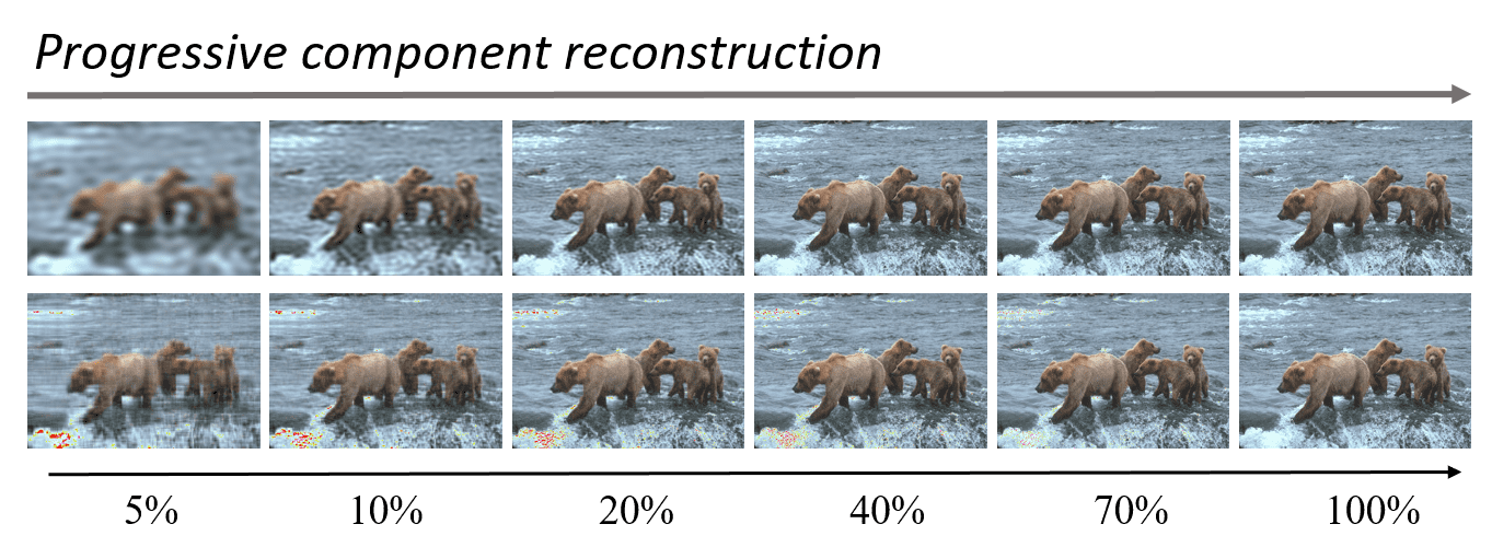
Figure 5: Visual comparison of the progressive reconstruction results with SVD and IDFT components, respectively. First row, IDFT reconstruction result. Second row, SVD reconstruction result. Both conform to the principle from outline to details.

where $X\in\mathbb{R}^{h\times w}$ represents the latent representation and $U\in\mathbb{R}^{h\times h}$, $V\in\mathbb{R}^{w\times w}$ represent the decomposed singular vectors with columns $u_{i}$, $v_{i}$, $k=min(h,w)$ denotes the rank of $X$. $\Sigma$ represents the singular values with diagonal elements $\sigma_{i}$. $G(u,v)$ denotes the coefficients of the fourier transform of $X$, and $\phi(u,v)$ denotes the corresponding two-dimensional wave component. Observing that both SVD and IDFT formation can be regarded as a weighted sum on a set of basis, i.e.$u_{i}v_{i}^{T}$ and $e^{j2\pi(\frac{um}{h}+\frac{vn}{w})}$, while the decomposed singular values $\sigma_{i}$ and the transformed fourier coefficients $G(u,v)$ inherently undertake the same role for the linear combination of various bases. In Fig. 5, we present the visualized comparison of the reconstruction results using partial components of SVD and IDFT progressively, while both formations conform to the principle from outline to details. Therefore, we presume that the SVD and IDFT operate in a similar way in terms of signal formation, and the combined coefficients $\sigma_{i}$ and $G(u,v)$ can be approximated to each other.

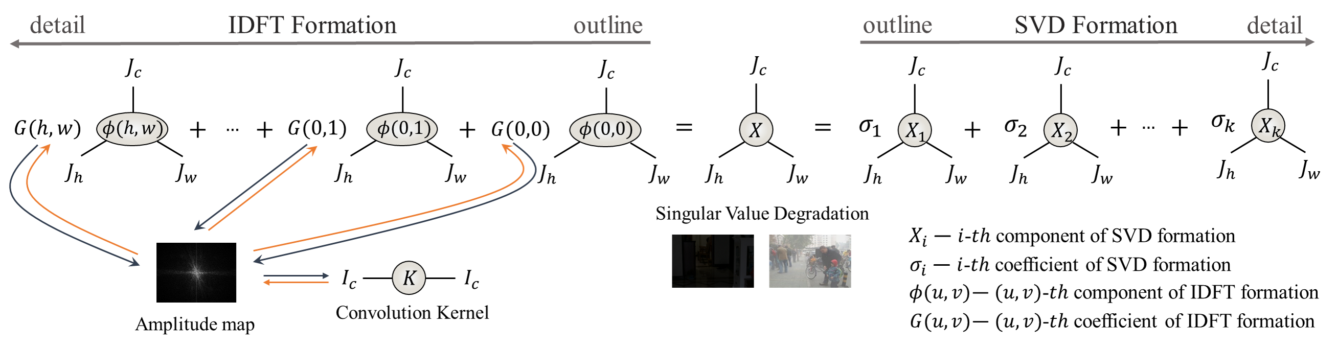
Figure 4: An illustration of the core idea of the proposed Singular Value Operator (SVAO), which is dedicated on the optimization of the singular value dominated degradations, i.e., haze and low-light. Two-dimensional signal formations are provided for simplicity.

TABLE I: Time comparison (ms) between SVD and FFT formation for signal representation on high-dimensional tensor, with supposed size $64\times 128\times 128$, where the Decom. and Comp. represent the decomposition and composition.

Formation	Decom. time	Comp.time	Total time
SVD	180.243	0.143	180.386
FFT	0.159	0.190	0.349

In this way, we successfully translate the unattainable singular values optimization to the accessible fourier coefficients optimization, as shown in Fig. 4. Considering the decomposed singular values typically characterize the global statistics of the signal, SVAO thus concentrates on the optimization of the norm of $G(u,v)$ for consistency, i.e.the amplitude map, since the phase of $G(u,v)$ implicitly represents the structural content [101, 100] and more in line with the singular vectors. The above two-dimensional signal formation can be easily extended to the three-dimensional tensor to perform the $1\times 1$ convolution. Since we adopt the SVAO merely in the bottleneck layers of the backbone network with low resolution inputs, and the fast fourier transform is substantially faster than the singular value decomposition; see Table I. The consequent overhead of SVAO can be greatly compressed. Note that the formation in Eq. 5 is a bit different from the definitive IDFT, and we provide the equivalence proof below.

Proof. For the two-dimensional signal $X\in\mathbb{R}^{h\times w}$, we can represent any point on it through IDFT. Supposing ($m$,$n$) and ($m^{{}^{\prime}}$, $n^{{}^{\prime}}$) are two random points on $X$, where $m$, $m^{{}^{\prime}}$ $\in$ [$0$, $h$-$1$], $n$, $n^{{}^{\prime}}$ $\in$ [$0$, $w$-$1$], and ($m$,$n$) $\neq$ ($m^{{}^{\prime}}$, $n^{{}^{\prime}}$), we have

$$X(m,n) =\frac{1}{hw}\sum_{u=0}^{h-1}\sum_{v=0}^{w-1}G(u,v)e^{j2\pi(\frac{um}{h}+\frac{vn}{w})},$$ (6)

$$X(m^{{}^{\prime}},n^{{}^{\prime}}) =\frac{1}{hw}\sum_{u=0}^{h-1}\sum_{v=0}^{w-1}G(u,v)e^{j2\pi(\frac{um^{{}^{\prime}}}{h}+\frac{vn^{{}^{\prime}}}{w})}.$$ (7)

$X(m,n)$ represents the signal value at ($m$,$n$) position on $X$, and the same as $X(m^{{}^{\prime}},n^{{}^{\prime}})$. Thus, we can rewrite $X$ as

$$X= \begin{bmatrix}X(0,0)&\cdots&X(0,w-1)\\ \vdots&\ddots&\vdots\\ X(h-1,0)&\cdots&X(h-1,w-1)\end{bmatrix}$$

$$= \frac{1}{hw}\sum_{u=0}^{h-1}\sum_{v=0}^{w-1}G(u,v)\;$$

$$\begin{bmatrix}e^{j2\pi(\frac{u0}{h}+\frac{v0}{w})}&\cdots&e^{j2\pi(\frac{u0}{h}+\frac{v(w-1)}{w})}\\ \vdots&\ddots&\vdots\\ e^{j2\pi(\frac{u(h-1)}{h}+\frac{v0}{w})}&\cdots&e^{j2\pi(\frac{u(h-1)}{h}+\frac{v(w-1)}{w})}\end{bmatrix}$$

$$= \frac{1}{hw}\sum_{u=0}^{h-1}\sum_{v=0}^{w-1}G(u,v)e^{j2\pi(\frac{um}{h}+\frac{vn}{w})},$$ (8)

where $m$ $\in\mathbb{R}^{h},n\in\mathbb{R}^{w}$. And the two-dimensional wave $e^{j2\pi(\frac{um}{h}+\frac{vn}{w})}\in\mathbb{R}^{h\times w}$ denotes the base component. Therefore, the formation principle of Eq. 5 is equivalent to the definitive IDFT, i.e.Eqs. 6 and 7. $\square$

III-D Optimization objective

The decomposition loss $\mathcal{L}_{dec}$ is developed to favor the decomposed optimization congruously, formulated as

$$\mathcal{L}_{dec}=\sum_{i=1}^{3}\beta\|U_{rec}^{(i)}V_{rec}^{(i)T}-U_{cle}^{(i)}V_{cle}^{(i)T}\|_{1}+\|\Sigma_{rec}^{(i)}-\Sigma_{cle}^{(i)}\|_{1},$$ (9)

where $U_{cle}$, $V_{cle}$, and $\Sigma_{cle}$ represent the decomposed singular vectors and singular values of the clean image, $U_{rec}$, $V_{rec}$, and $\Sigma_{rec}$ represent the decomposed singular vectors and singular values of the recovered image. For simplicity, we omit the pseudo identity matrix between $UV^{T}$ for dimension transformation. $\beta$ denotes the weight.

The overall optimization objective of DASL comprises the orthogonal regularization loss $\mathcal{L}_{orth}$ and the decomposition loss $\mathcal{L}_{dec}$, together with the original loss functions of the integrated backbone network $\mathcal{L}_{ori}$, formulated as

$$\mathcal{L}_{total}=\mathcal{L}_{ori}+\lambda_{orth}\mathcal{L}_{orth}+\lambda_{dec}\mathcal{L}_{dec},$$ (10)

where $\lambda_{orth}$ and $\lambda_{dec}$ denote the balanced weights.

IV Experiments

In this section, we first clarify the experimental settings, and then present the qualitative and quantitative comparison results with eleven baseline methods for unified image restoration. Moreover, extensive ablation experiments are conducted to verify the effectiveness of our method.

TABLE II: Quantitative results on five common image restoration datasets with state-of-the-art general image restoration methods and all-in-one image restoration methods. The baseline results are in grey.

	Rain100L [77]		BSD68 [78]		GoPro [89]		SOTS [75]		LOL [90]		Average		Params
Method	PSNR$\uparrow$	SSIM$\uparrow$	PSNR$\uparrow$	SSIM$\uparrow$	PSNR$\uparrow$	SSIM$\uparrow$	PSNR$\uparrow$	SSIM$\uparrow$	PSNR$\uparrow$	SSIM$\uparrow$	PSNR$\uparrow$	SSIM$\uparrow$
NAFNet [10]	35.56	0.967	31.02	0.883	26.53	0.808	25.23	0.939	20.49	0.809	27.76	0.881	17.11M
HINet [11]	35.67	0.969	31.00	0.881	26.12	0.788	24.74	0.937	19.47	0.800	27.40	0.875	88.67M
MIRNetV2 [92]	33.89	0.954	30.97	0.881	26.30	0.799	24.03	0.927	21.52	0.815	27.34	0.875	5.86M
SwinIR [28]	30.78	0.923	30.59	0.868	24.52	0.773	21.50	0.891	17.81	0.723	25.04	0.835	0.91M
Restormer [13]	34.81	0.962	31.49	0.884	27.22	0.829	24.09	0.927	20.41	0.806	27.60	0.881	26.13M
MPRNet [14]	38.16	0.981	31.35	0.889	26.87	0.823	24.27	0.937	20.84	0.824	28.27	0.890	15.74M
DGUNet [25]	36.62	0.971	31.10	0.883	27.25	0.837	24.78	0.940	21.87	0.823	28.32	0.891	17.33M
DL [24]	21.96	0.762	23.09	0.745	19.86	0.672	20.54	0.826	19.83	0.712	21.05	0.743	2.09M
Transweather [16]	29.43	0.905	29.00	0.841	25.12	0.757	21.32	0.885	21.21	0.792	25.22	0.836	37.93M
TAPE [27]	29.67	0.904	30.18	0.855	24.47	0.763	22.16	0.861	18.97	0.621	25.09	0.801	1.07M
AirNet [20]	32.98	0.951	30.91	0.882	24.35	0.781	21.04	0.884	18.18	0.735	25.49	0.846	8.93M
DASL+MPRNet	38.02	0.980	31.57	0.890	26.91	0.823	25.82	0.947	20.96	0.826	28.66	0.893	15.15M
DASL+DGUNet	36.96	0.972	31.23	0.885	27.23	0.836	25.33	0.943	21.78	0.824	28.51	0.892	16.92M
DASL+AirNet	34.93	0.961	30.99	0.883	26.04	0.788	23.64	0.924	20.06	0.805	27.13	0.872	5.41M

IV-A Implementation Details

Tasks and Metrics. We train our method on five image restoration tasks synchronously. The corresponding training set includes Rain200L [77] for image deraining, RESIDE-OTS [75] for image dehazing, BSD400 [78], WED [76] for image denoising, GoPro [89] for image deblurring, and LOL [90] for low-light image enhancement. For evaluation, 100 image pairs in Rain100L [77], 500 image pairs in SOTS-Outdoor [75], total 192 images in BSD68 [78], Urban100 [79] and Kodak24 [93], 1111 image pairs in GoPro [89], 15 image pairs in LOL [90] are utilized as the test set. We report the Peak Signal to Noise Ratio (PSNR) and Structural Similarity (SSIM) as evaluation metrics for numerical comparison in our experiments.

Training. We implement our method on single NVIDIA Geforce RTX 3090 GPU. For fair comparison, all comparison methods have been retrained in the new mixed dataset with their default hyperparameter settings. The entire network is trained with Adam optimizer for 1200 epochs. We set the batch size as 8 and random crop 128x128 patch from the original image as network input after data augmentation. We set the $\beta$ in $\mathcal{L}_{dec}$ as 0.01, and the $\lambda_{orth}$, $\lambda_{dec}$ are set to be 1e-4 and 0.1, respectively. We perform evaluations every 20 epochs with the highest average PSNR scores as the final parameters result.

Model details. We implement our DASL with integrated MPRNet [14], DGUNet [25], and AirNet [20] backbone to validate the effectiveness of the decomposed optimization. Fig. 7 (a) presents the cascading working mechanism of our operator. Note that the SVAO is only adopted in the bottleneck layer, as described in Sec. III-A. We introduce how we embed our operator into the backbone network from a microscopic perspective. Sincerely, the most convenient way is to directly reform the basic block of the backbone network. We present two fashions of the basic block of baseline in Fig. 7 (b) and (c), where the MPRNet fashion is composed of two basic units, e.g., channel attention block (CAB) [99], and DGUNet is constructed by two vanilla activated convolutions. We simply replace one of them (dashed line) with our operator to realize the DASL integration. Note that AirNet shares the similar fashion as MPRNet and we omit it for simplicity.

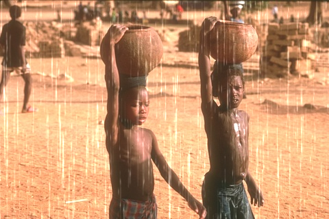
(a) Rainy Image

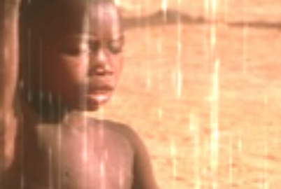
(b) Rainy

(c) NAFNet [10]

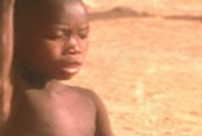
(d) HINet [11]

(e) MPRNet [14]

(f) DGUNet [25]

(g) MIRNetV2 [92]

(h) Transweather [16]

(i) SwinIR [28]

(j) TAPE [27]

(k) DL [24]

(l) Restormer [13]

(m) AirNet [20]

(n) DASL+MPRNet

(o) GT

Figure 6: Visual comparison with state-of-the-art methods on Rain100L dataset. Please zoom in for details.

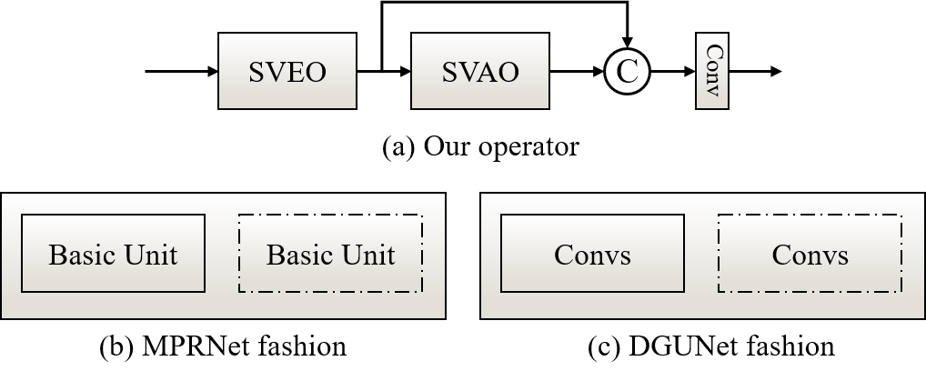
Figure 7: The strategy of model integration with DASL. (a) The working mechanism of our operator. (b) The basic building block of MPRNet. (c) The basic building block of DGUNet.

IV-B Comparison with state-of-the-art methods

We compare our DASL with eleven state-of-the-art methods, including general image restoration methods: NAFNet [10], HINet [11], MPRNet [14], DGUNet [25], MIRNetV2 [92], SwinIR [28], Restormer [13], and all-in-one fashion methods: DL [24], Transweather [16], TAPE [27] and AirNet [20] on five common image restoration tasks.

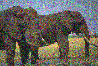
(a) Noisy Image

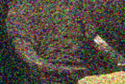
(b) Noisy

(c) NAFNet [10]

(d) HINet [11]

(e) MPRNet [14]

(f) DGUNet [25]

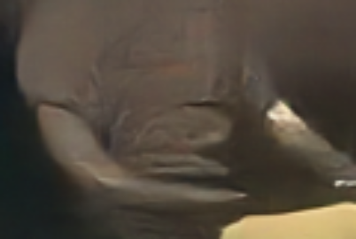
(g) MIRNetV2 [92]

(h) Transweather [16]

(i) SwinIR [28]

(j) TAPE [27]

(k) DL [24]

(l) Restormer [13]

(m) AirNet [20]

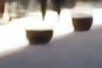
(n) DASL+MPRNet

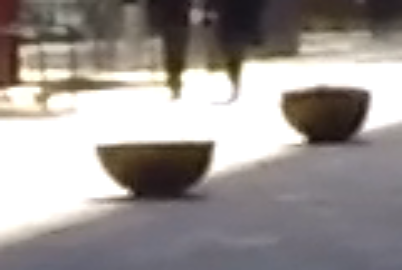
(o) GT

Figure 8: Visual comparison with state-of-the-art methods on BSD68 dataset. Please zoom in for details.

Table II reports the quantitative comparison results. It can be observed that the performance of the general image restoration methods is systematically superior to the professional all-in-one fashion methods when more degradations are involved, attributed to the large model size. While our DASL further advances the backbone network capability with fewer parameters, owing to the implicit synergistic learning. Consistent with existing unified image restoration methods [13, 20], we report the detailed denoising results at different noise ratio in Table III, where the performance gain are consistent.

TABLE III: Quantitative results of image denoising on BSD68, Urban100 and Set12 datasets in terms of PSNR$\uparrow$.

	BSD68 [78]			Urban100 [79]			Kodak24 [93]
Method	$\sigma$=15	$\sigma$=25	$\sigma$=50	$\sigma$=15	$\sigma$=25	$\sigma$=50	$\sigma$=15	$\sigma$=25	$\sigma$=50
NAFNet [10]	33.67	31.02	27.73	33.14	30.64	27.20	34.27	31.80	28.62
HINet [11]	33.72	31.00	27.63	33.49	30.94	27.32	34.38	31.84	28.52
MIRNetV2 [92]	33.66	30.97	27.66	33.30	30.75	27.22	34.29	31.81	28.55
SwinIR [28]	33.31	30.59	27.13	32.79	30.18	26.52	33.89	31.32	27.93
Restormer [13]	34.03	31.49	28.11	33.72	31.26	28.03	34.78	32.37	29.08
MPRNet [14]	34.01	31.35	28.08	34.13	31.75	28.41	34.77	32.31	29.11
DGUNet [25]	33.85	31.10	27.92	33.67	31.27	27.94	34.56	32.10	28.91
DL [24]	23.16	23.09	22.09	21.10	21.28	20.42	22.63	22.66	21.95
Transweather [16]	31.16	29.00	26.08	29.64	27.97	26.08	31.67	29.64	26.74
TAPE [27]	32.86	30.18	26.63	32.19	29.65	25.87	33.24	30.70	27.19
AirNet [20]	33.49	30.91	27.66	33.16	30.83	27.45	34.14	31.74	28.59
DASL+MPRNet	34.16	31.57	28.18	34.21	31.82	28.47	34.91	32.46	29.18
DASL+DGUNet	33.94	31.23	27.94	33.74	31.31	27.96	34.69	32.16	28.93
DASL+AirNet	33.69	30.99	27.68	33.35	30.89	27.46	34.32	31.79	28.61

TABLE IV: Comparison of the model size and computation complexity between baseline / DASL.

Method	Params (M)	FLOPs (B)	Inference Time (s)
MPRNet	15.74 / 15.15	5575.32 / 2905.14	0.241 / 0.210
DGUNet	17.33 / 16.92	3463.66 / 3020.22	0.397 / 0.391
AirNet	8.93 / 5.41	1205.09 / 767.89	0.459 / 0.190

In  Table IV, we present the computation overhead involved in DASL, where the FLOPs and inference time are calculated over 100 testing images with the size of 512×512. It can be observed that our DASL substantially reduce the computation complexity of the baseline methods with considerable inference acceleration, e.g.12.86% accelerated on MPRNet and 58.61% accelerated on AirNet. Note that DASL is integrated into the existing backbone network through the replacement operation instead of attachment, demonstrating its efficiency.

(a) Blurry Image

(b) Blurry

(c) NAFNet [10]

(d) HINet [11]

(e) MPRNet [14]

(f) DGUNet [25]

(g) MIRNetV2 [92]

(h) Transweather [16]

(i) SwinIR [28]

(j) TAPE [27]

(k) DL [24]

(l) Restormer [13]

(m) AirNet [20]

(n) DASL+MPRNet

(o) GT

Figure 9: Visual comparison with state-of-the-art methods on GoPro dataset. Please zoom in for details.

TABLE V: Ablation experiments of scale ratio $r$ in the SVEO (PSNR$\uparrow$).

scale ratio $r$	Rain100L	SOTS	GoPro	BSD68	LOL
1	38.01	31.55	26.88	25.84	20.93
2	38.02	31.57	26.91	25.82	20.96
4	38.07	31.58	26.92	25.81	20.98

We present the visual comparison results of aforementioned image restoration tasks in Figs. 6, 8, 9, 10 and 11, including singular vector dominated degradations rain, noise, blur, and singular value dominated degradations low-light, haze. It can be observed that our DASL exhibits superior visual recovery quality in both types of degradation, i.e.more precise content details in singular vector dominated degradations and more stable global recovery in singular value dominated degradations, compared to the integrated baseline method.

IV-C Ablation Studies

We present the ablation experiments on the combined degradation dataset with MPRNet as the backbone to verify the effectiveness of our method. In Table VII, we quantitatively evaluate the two developed operators SVEO and SVAO, and the decomposition loss. The metrics are reported on the each of degradations in detail, from which we can make the following observations:

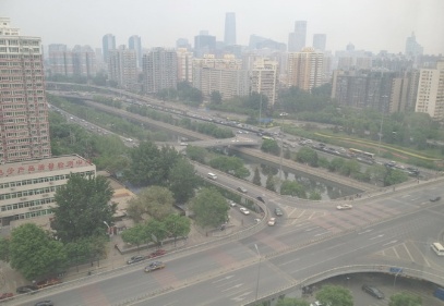
(a) Hazy Image

(b) Hazy

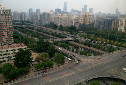
(c) NAFNet [10]

(d) HINet [11]

(e) MPRNet [14]

(f) DGUNet [25]

(g) MIRNetV2 [92]

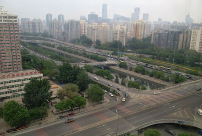
(h) Transweather [16]

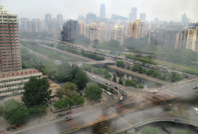
(i) SwinIR [28]

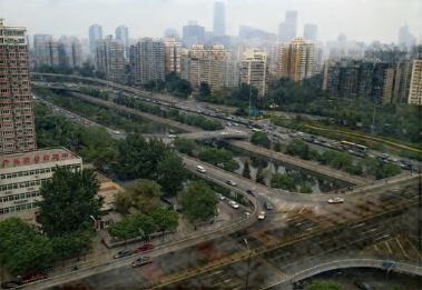
(j) TAPE [27]

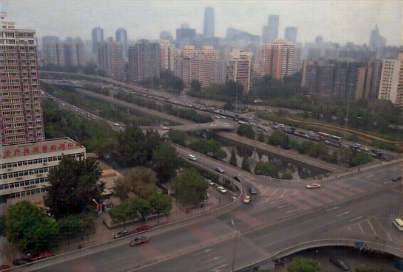
(k) DL [24]

(l) Restormer [13]

(m) AirNet [20]

(n) DASL+MPRNet

(o) GT

Figure 10: Visual comparison with state-of-the-art methods on SOTS dataset. Please zoom in for details.

TABLE VI: Evaluating the scalability of decomposed optimization with partial training degradations (PSNR$\uparrow$).

Tasks	Rain100L	BSD68	GoPro	SOTS	LOL
MPRNet (vec.)	39.47	31.50	27.61	15.91	7.77
MPRNet (val.)	-	-	-	-	-
DGUNet (vec.)	39.04	31.46	28.22	15.92	7.76
DGUNet (val.)	23.10	20.39	21.84	24.59	20.45
AirNet (vec.)	36.62	31.33	26.35	15.90	7.75
AirNet (val.)	19.52	19.17	14.47	20.63	16.01
DASL+MPRNet (vec.)	39.39	31.63	27.57	17.21	11.23
DASL+MPRNet (val.)	21.87	19.96	21.35	25.13	20.33
DASL+DGUNet (vec.)	39.11	31.55	28.16	16.87	10.21
DASL+DGUNet (val.)	23.19	20.28	22.69	25.05	20.87
DASL+AirNet (vec.)	36.87	31.22	26.72	15.97	8.77
DASL+AirNet (val.)	21.25	20.38	21.12	24.60	20.58

TABLE VII: Ablation experiments on the components design.

					Rain100L [77]		BSD68 [78]		GoPro [89]		SOTS [75]		LOL [90]
Method	SVEO	SVAO	$\mathcal{L}_{orth}$	$\mathcal{L}_{dec}$	PSNR$\uparrow$	SSIM$\uparrow$	PSNR$\uparrow$	SSIM$\uparrow$	PSNR$\uparrow$	SSIM$\uparrow$	PSNR$\uparrow$	SSIM$\uparrow$	PSNR$\uparrow$	SSIM$\uparrow$
Baseline					38.16	0.981	31.35	0.889	26.87	0.823	24.27	0.937	20.84	0.824
With no orth. SVEO	✓				37.73	0.981	31.31	0.889	26.79	0.819	24.63	0.939	20.83	0.824
With SVAO		✓			37.92	0.980	31.41	0.889	26.85	0.821	25.58	0.943	21.05	0.828
With SVEO	✓		✓		38.04	0.981	31.46	0.890	26.97	0.826	25.53	0.945	20.76	0.822
With SVEO and SVAO	✓	✓	✓		38.01	0.980	31.53	0.890	26.94	0.825	25.63	0.948	20.92	0.826
With $\mathcal{L}_{dec}$				✓	38.10	0.982	31.39	0.889	26.78	0.819	24.70	0.942	20.98	0.827
DASL+MPRNet	✓	✓	✓	✓	38.02	0.980	31.57	0.890	26.91	0.823	25.82	0.947	20.96	0.826

a) Both SVEO and SVAO are quite beneficial for advancing the unified degradation restoration performance, attributing to the ascribed synergistic learning. b) The congruous decomposition loss is capable to work alone, and well collaborated with the developed operators for decomposed optimization. c) The orthogonal regularization is crucial to prevent the potential performance drop of SVEO, ensuring the reliable optimization.

To further verify the scalability of the decomposed optimization, Table VI evaluates the performance with merely trained on singular vector dominated degradations (vec.) and singular value dominated degradations (val.). While some intriguing properties have been observed: a) Basically, the baseline methods concentrate on the trainable degradations, while our DASL further contemplates the untrainable ones in virtue of its slight task dependency. b) The performance of MPRNet on val. is unattainable due to the non-convergence, however, our DASL successfully circumvents this drawback owing to the dedicated decomposed optimization on singular values rather than task-level learning. c) The vec. seems to be supportive to the restoration performance of val., see the comparison of Tables II and VI, indicating the potential relationship among the decomposed two types of degradations.

We present the comparison of the training trajectory between baseline and DASL on singular vector dominated degradations and singular value dominated degradations in Figs. 12 and 13. It can be observed that our DASL significantly suppresses the drastic optimization process, and retain the overall steady to better convergence point with even fewer parameters, attributing to the ascribed synergistic learning

IV-D Limitation and Future works

Despite the great progress that DASL has been made in ascribing the implicit relationship among diverse degradations for synergistic learning, the more sophisticated correlations demand further investigation. We notice that beyond the decomposed singular vectors and singular values, the distribution discrepancy of various degradations on separate order decomposed components exhibits the splendid potential, which can be glimpsed from Fig. 2. Additionally, how to leverage and represent their sophisticated relationship in a unified framework remains an open problem.

(a) Low-light Image

(b) Low-light

(c) NAFNet [10]

(d) HINet [11]

(e) MPRNet [14]

(f) DGUNet [25]

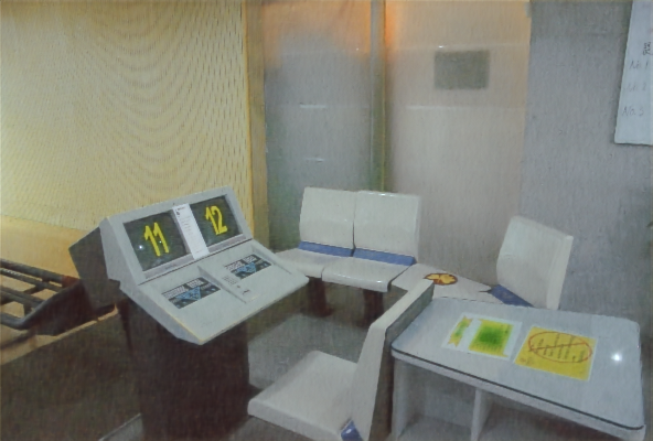
(g) MIRNetV2 [92]

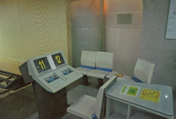
(h) Transweather [16]

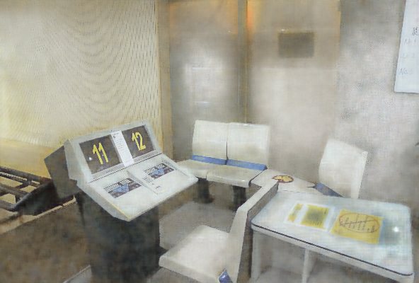
(i) SwinIR [28]

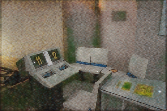
(j) TAPE [27]

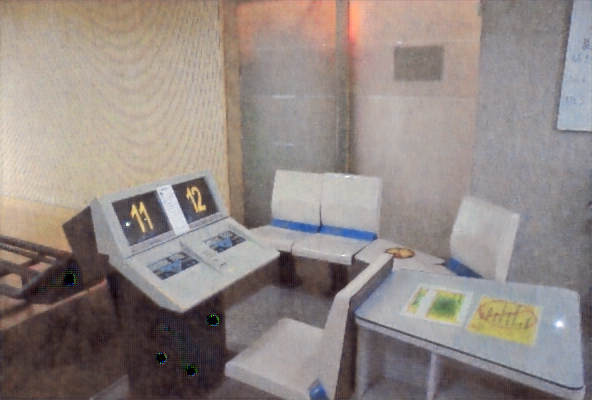
(k) DL [24]

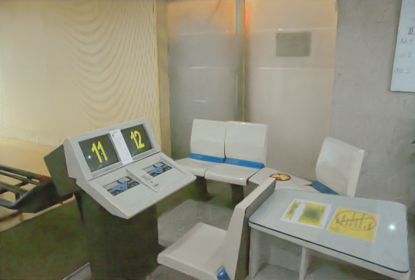
(l) Restormer [13]

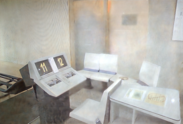
(m) AirNet [20]

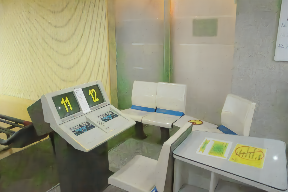
(n) DASL+MPRNet

(o) GT

Figure 11: Visual comparison with state-of-the-art methods on LOL dataset. Please zoom in for details.

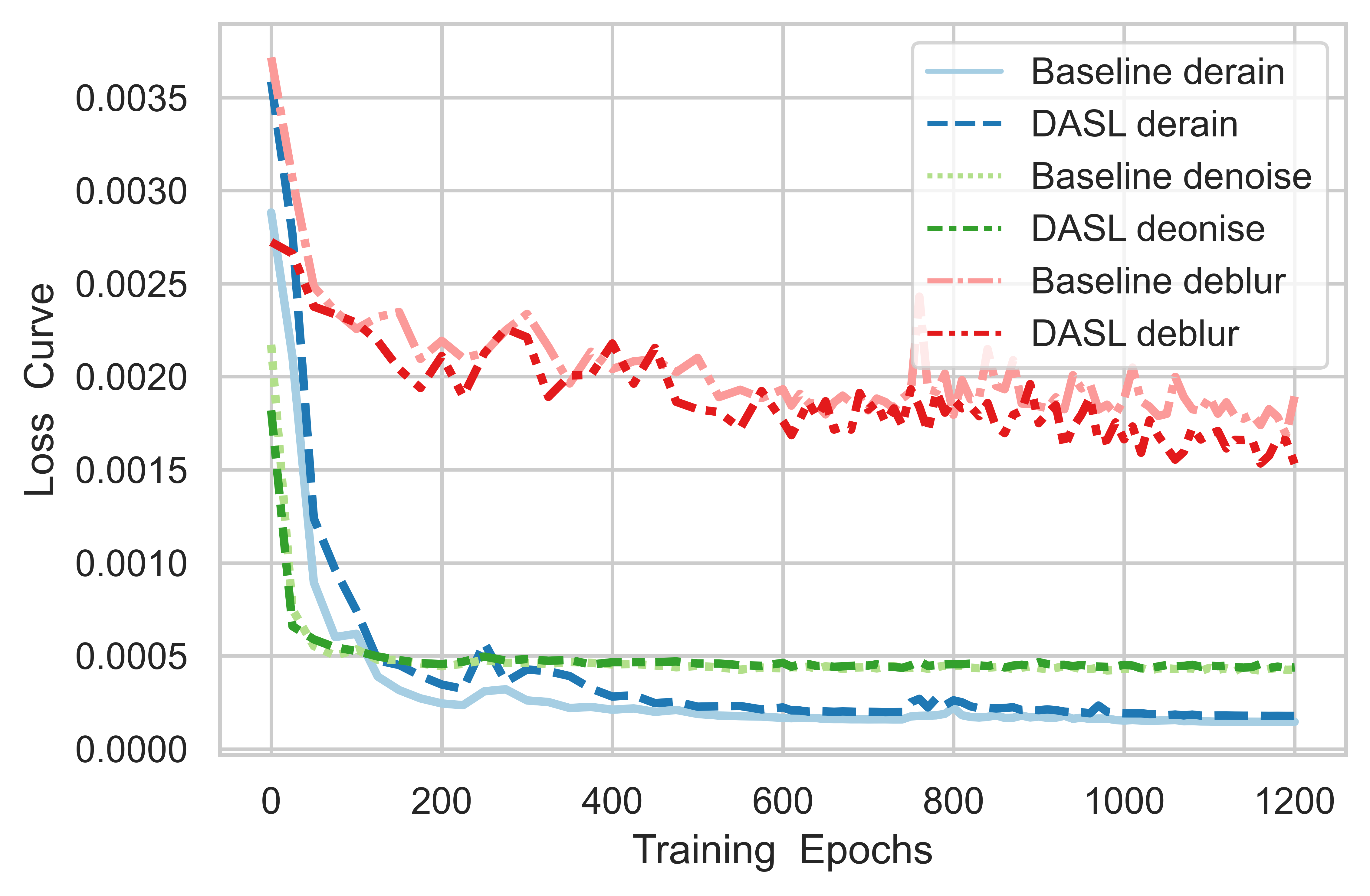
Figure 12: Comparison of the training trajectory between baseline method and DASL on singular vector dominated degradations.

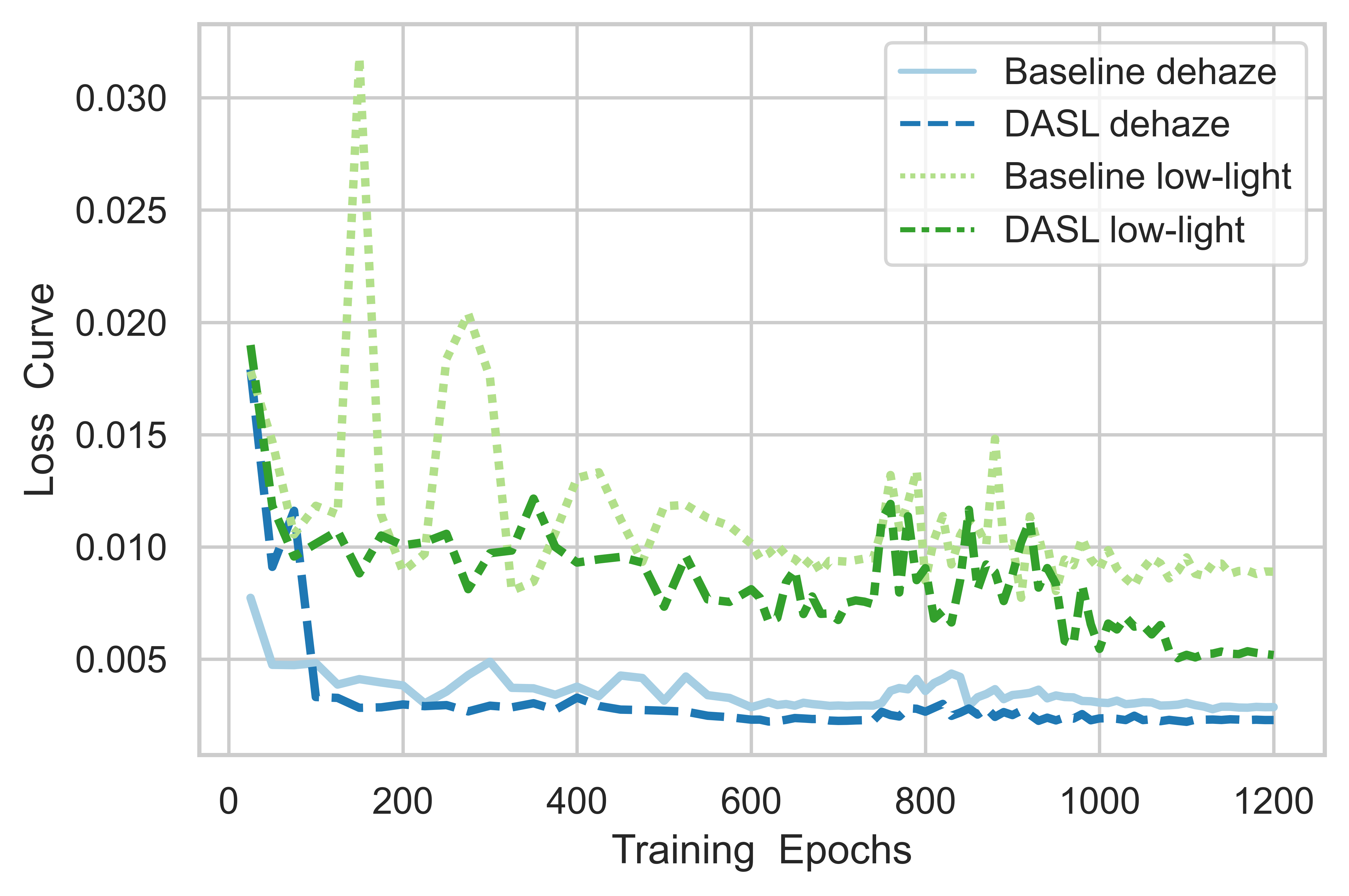
Figure 13: Comparison of the training trajectory between baseline method and DASL on singular value dominated degradations.

V Conclusion

In this paper, we revisit the diverse degradations through the lens of singular value decomposition to excavate their relationship, and observed that the decomposed singular vectors and singular values naturally undertake the different types of degradation information, ascribing various restoration tasks into two groups, i.e.singular vector dominated and singular value dominated. The proposed Decomposition Ascribed Synergistic Learning dedicates the decomposed optimization of degraded singular vectors and singular values respectively, rendering a more unified perspective to inherently utilize the potential relationship among diverse restoration tasks. Two effective operators SVEO and SVAO have been developed to favor the decomposed optimization, along with a congruous decomposition loss, which can be lightly integrated into existing convolutional image restoration backbone. Extensive experiments on blended five image restoration tasks validate the effectiveness of the proposed method.

References

- [1] C. Li, C.-L. Guo, M. Zhou, Z. Liang, S. Zhou, R. Feng, and C. C. Loy, “Embeddingfourier for ultra-high-definition low-light image enhancement,” in ICLR, 2023.
- [2] J. Lehtinen, J. Munkberg, J. Hasselgren, S. Laine, T. Karras, M. Aittala, and T. Aila, “Noise2noise: Learning image restoration without clean data,” in International Conference on Machine Learning. PMLR, 2018, pp. 2965–2974.
- [3] D. Kundur and D. Hatzinakos, “Blind image deconvolution,” IEEE signal processing magazine, vol. 13, no. 3, pp. 43–64, 1996.
- [4] M. I. Sezan and A. M. Tekalp, “Survey of recent developments in digital image restoration,” Optical Engineering, vol. 29, no. 5, pp. 393–404, 1990.
- [5] K. He, J. Sun, and X. Tang, “Single image haze removal using dark channel prior,” IEEE transactions on pattern analysis and machine intelligence, vol. 33, no. 12, pp. 2341–2353, 2010.
- [6] S. D. Babacan, R. Molina, and A. K. Katsaggelos, “Variational bayesian blind deconvolution using a total variation prior,” IEEE Transactions on Image Processing, vol. 18, no. 1, pp. 12–26, 2008.
- [7] M. Zhou, H. Yu, J. Huang, F. Zhao, J. Gu, C. C. Loy, D. Meng, and C. Li, “Deep fourier up-sampling,” in Advances in Neural Information Processing Systems, 2022.
- [8] Y. Cui, Y. Tao, Z. Bing, W. Ren, X. Gao, X. Cao, K. Huang, and A. Knoll, “Selective frequency network for image restoration,” in International Conference on Learning Representations, 2023.
- [9] D. Ulyanov, A. Vedaldi, and V. Lempitsky, “Deep image prior,” in Proceedings of the IEEE conference on computer vision and pattern recognition, 2018, pp. 9446–9454.
- [10] L. Chen, X. Chu, X. Zhang, and J. Sun, “Simple baselines for image restoration,” in European Conference on Computer Vision. Springer, 2022, pp. 17–33.
- [11] L. Chen, X. Lu, J. Zhang, X. Chu, and C. Chen, “Hinet: Half instance normalization network for image restoration,” in Proceedings of the IEEE/CVF Conference on Computer Vision and Pattern Recognition, 2021, pp. 182–192.
- [12] J. Pan, S. Liu, D. Sun, J. Zhang, Y. Liu, J. Ren, Z. Li, J. Tang, H. Lu, Y.-W. Tai et al., “Learning dual convolutional neural networks for low-level vision,” in Proceedings of the IEEE conference on computer vision and pattern recognition, 2018, pp. 3070–3079.
- [13] S. W. Zamir, A. Arora, S. Khan, M. Hayat, F. S. Khan, and M.-H. Yang, “Restormer: Efficient transformer for high-resolution image restoration,” in Proceedings of the IEEE/CVF Conference on Computer Vision and Pattern Recognition, 2022, pp. 5728–5739.
- [14] S. W. Zamir, A. Arora, S. Khan, M. Hayat, F. S. Khan, M.-H. Yang, and L. Shao, “Multi-stage progressive image restoration,” in Proceedings of the IEEE/CVF conference on computer vision and pattern recognition, 2021, pp. 14 821–14 831.
- [15] H. Chen, Y. Wang, T. Guo, C. Xu, Y. Deng, Z. Liu, S. Ma, C. Xu, C. Xu, and W. Gao, “Pre-trained image processing transformer,” in Proceedings of the IEEE/CVF Conference on Computer Vision and Pattern Recognition, 2021, pp. 12 299–12 310.
- [16] J. M. J. Valanarasu, R. Yasarla, and V. M. Patel, “Transweather: Transformer-based restoration of images degraded by adverse weather conditions,” in Proceedings of the IEEE/CVF Conference on Computer Vision and Pattern Recognition, 2022, pp. 2353–2363.
- [17] W.-T. Chen, Z.-K. Huang, C.-C. Tsai, H.-H. Yang, J.-J. Ding, and S.-Y. Kuo, “Learning multiple adverse weather removal via two-stage knowledge learning and multi-contrastive regularization: Toward a unified model,” in Proceedings of the IEEE/CVF Conference on Computer Vision and Pattern Recognition, 2022, pp. 17 653–17 662.
- [18] Z. Zhang, S. Zhao, X. Jin, M. Xu, Y. Yang, and S. Yan, “Noiser: Noise is all you need for enhancing low-light images without task-related data,” arXiv preprint arXiv:2211.04700, 2022.
- [19] Z. Zhang, R. Xu, M. Liu, Z. Yan, and W. Zuo, “Self-supervised image restoration with blurry and noisy pairs,” in Advances in Neural Information Processing Systems.
- [20] B. Li, X. Liu, P. Hu, Z. Wu, J. Lv, and X. Peng, “All-in-one image restoration for unknown corruption,” in Proceedings of the IEEE/CVF Conference on Computer Vision and Pattern Recognition, 2022, pp. 17 452–17 462.
- [21] W. Wang, B. Li, Y. Gou, P. Hu, and X. Peng, “Relationship quantification of image degradations,” arXiv preprint arXiv:2212.04148, 2022.
- [22] R. Li, R. T. Tan, and L.-F. Cheong, “All in one bad weather removal using architectural search,” in Proceedings of the IEEE/CVF conference on computer vision and pattern recognition, 2020, pp. 3175–3185.
- [23] S. Chen, T. Ye, Y. Liu, and E. Chen, “Dual-former: Hybrid self-attention transformer for efficient image restoration,” arXiv preprint arXiv:2210.01069, 2022.
- [24] Q. Fan, D. Chen, L. Yuan, G. Hua, N. Yu, and B. Chen, “A general decoupled learning framework for parameterized image operators,” IEEE transactions on pattern analysis and machine intelligence, vol. 43, no. 1, pp. 33–47, 2019.
- [25] C. Mou, Q. Wang, and J. Zhang, “Deep generalized unfolding networks for image restoration,” in Proceedings of the IEEE/CVF Conference on Computer Vision and Pattern Recognition, 2022, pp. 17 399–17 410.
- [26] X. Fu, Z. Xiao, G. Yang, A. Liu, Z. Xiong et al., “Unfolding taylor’s approximations for image restoration,” Advances in Neural Information Processing Systems, vol. 34, pp. 18 997–19 009, 2021.
- [27] L. Liu, L. Xie, X. Zhang, S. Yuan, X. Chen, W. Zhou, H. Li, and Q. Tian, “Tape: Task-agnostic prior embedding for image restoration,” in European Conference on Computer Vision. Springer, 2022, pp. 447–464.
- [28] J. Liang, J. Cao, G. Sun, K. Zhang, L. Van Gool, and R. Timofte, “Swinir: Image restoration using swin transformer,” in Proceedings of the IEEE/CVF International Conference on Computer Vision, 2021, pp. 1833–1844.
- [29] Z. Wang, X. Cun, J. Bao, W. Zhou, J. Liu, and H. Li, “Uformer: A general u-shaped transformer for image restoration,” in Proceedings of the IEEE/CVF Conference on Computer Vision and Pattern Recognition, 2022, pp. 17 683–17 693.
- [30] C. Guo, C. Li, J. Guo, C. C. Loy, J. Hou, S. Kwong, and R. Cong, “Zero-reference deep curve estimation for low-light image enhancement,” in Proceedings of the IEEE/CVF Conference on Computer Vision and Pattern Recognition, 2020, pp. 1780–1789.
- [31] W. Wu, J. Weng, P. Zhang, X. Wang, W. Yang, and J. Jiang, “Uretinex-net: Retinex-based deep unfolding network for low-light image enhancement,” in Proceedings of the IEEE/CVF Conference on Computer Vision and Pattern Recognition, 2022, pp. 5901–5910.
- [32] L. Ma, T. Ma, R. Liu, X. Fan, and Z. Luo, “Toward fast, flexible, and robust low-light image enhancement,” in Proceedings of the IEEE/CVF Conference on Computer Vision and Pattern Recognition, 2022, pp. 5637–5646.
- [33] Z. Zheng, W. Ren, X. Cao, X. Hu, T. Wang, F. Song, and X. Jia, “Ultra-high-definition image dehazing via multi-guided bilateral learning,” in 2021 IEEE/CVF Conference on Computer Vision and Pattern Recognition (CVPR). IEEE, 2021, pp. 16 180–16 189.
- [34] B. Li, X. Peng, Z. Wang, J. Xu, and D. Feng, “Aod-net: All-in-one dehazing network,” in Proceedings of the IEEE international conference on computer vision, 2017, pp. 4770–4778.
- [35] X. Qin, Z. Wang, Y. Bai, X. Xie, and H. Jia, “Ffa-net: Feature fusion attention network for single image dehazing,” in Proceedings of the AAAI Conference on Artificial Intelligence, vol. 34, no. 07, 2020, pp. 11 908–11 915.
- [36] Y. Song, Z. He, H. Qian, and X. Du, “Vision transformers for single image dehazing,” IEEE Transactions on Image Processing, vol. 32, pp. 1927–1941, 2023.
- [37] J. Pan, H. Bai, and J. Tang, “Cascaded deep video deblurring using temporal sharpness prior,” in Proceedings of the IEEE/CVF Conference on Computer Vision and Pattern Recognition, 2020, pp. 3043–3051.
- [38] S.-J. Cho, S.-W. Ji, J.-P. Hong, S.-W. Jung, and S.-J. Ko, “Rethinking coarse-to-fine approach in single image deblurring,” in Proceedings of the IEEE/CVF international conference on computer vision, 2021, pp. 4641–4650.
- [39] S. Nah, S. Son, S. Lee, R. Timofte, and K. M. Lee, “Ntire 2021 challenge on image deblurring,” in Proceedings of the IEEE/CVF Conference on Computer Vision and Pattern Recognition, 2021, pp. 149–165.
- [40] Y. Ye, Y. Chang, H. Zhou, and L. Yan, “Closing the loop: Joint rain generation and removal via disentangled image translation,” in Proceedings of the IEEE/CVF Conference on Computer Vision and Pattern Recognition, 2021, pp. 2053–2062.
- [41] J. Xiao, X. Fu, A. Liu, F. Wu, and Z.-J. Zha, “Image de-raining transformer,” IEEE Transactions on Pattern Analysis and Machine Intelligence, 2022.
- [42] K. Jiang, Z. Wang, P. Yi, C. Chen, B. Huang, Y. Luo, J. Ma, and J. Jiang, “Multi-scale progressive fusion network for single image deraining,” in Proceedings of the IEEE/CVF conference on computer vision and pattern recognition, 2020, pp. 8346–8355.
- [43] K. Zhang, W. Zuo, Y. Chen, D. Meng, and L. Zhang, “Beyond a gaussian denoiser: Residual learning of deep cnn for image denoising,” IEEE transactions on image processing, vol. 26, no. 7, pp. 3142–3155, 2017.
- [44] W. Lee, S. Son, and K. M. Lee, “Ap-bsn: Self-supervised denoising for real-world images via asymmetric pd and blind-spot network,” in Proceedings of the IEEE/CVF Conference on Computer Vision and Pattern Recognition, 2022, pp. 17 725–17 734.
- [45] S. Guo, Z. Yan, K. Zhang, W. Zuo, and L. Zhang, “Toward convolutional blind denoising of real photographs,” in Proceedings of the IEEE/CVF conference on computer vision and pattern recognition, 2019, pp. 1712–1722.
- [46] S. Jie and Z.-H. Deng, “Fact: Factor-tuning for lightweight adaptation on vision transformer,” arXiv preprint arXiv:2212.03145, 2022.
- [47] A. Obukhov, M. Usvyatsov, C. Sakaridis, K. Schindler, and L. Van Gool, “Tt-nf: Tensor train neural fields,” arXiv preprint arXiv:2209.15529, 2022.
- [48] K. Sozykin, A. Chertkov, R. Schutski, A.-H. PHAN, A. Cichocki, and I. Oseledets, “Ttopt: A maximum volume quantized tensor train-based optimization and its application to reinforcement learning,” in Advances in Neural Information Processing Systems.
- [49] M. Kanakis, D. Bruggemann, S. Saha, S. Georgoulis, A. Obukhov, and L. Van Gool, “Reparameterizing convolutions for incremental multi-task learning without task interference,” in Computer Vision–ECCV 2020: 16th European Conference. Springer, 2020, pp. 689–707.
- [50] A. Obukhov, M. Rakhuba, S. Georgoulis, M. Kanakis, D. Dai, and L. Van Gool, “T-basis: a compact representation for neural networks,” in International Conference on Machine Learning. PMLR, 2020, pp. 7392–7404.
- [51] K. Wang, Y. Wang, X.-L. Zhao, J. C.-W. Chan, Z. Xu, and D. Meng, “Hyperspectral and multispectral image fusion via nonlocal low-rank tensor decomposition and spectral unmixing,” IEEE Transactions on Geoscience and Remote Sensing, vol. 58, no. 11, pp. 7654–7671, 2020.
- [52] J. Peng, Y. Wang, H. Zhang, J. Wang, and D. Meng, “Exact decomposition of joint low rankness and local smoothness plus sparse matrices,” IEEE Transactions on Pattern Analysis and Machine Intelligence, 2022.
- [53] Y. Wang, J. Peng, Q. Zhao, Y. Leung, X.-L. Zhao, and D. Meng, “Hyperspectral image restoration via total variation regularized low-rank tensor decomposition,” IEEE Journal of Selected Topics in Applied Earth Observations and Remote Sensing, vol. 11, no. 4, pp. 1227–1243, 2017.
- [54] Y. Peng, D. Meng, Z. Xu, C. Gao, Y. Yang, and B. Zhang, “Decomposable nonlocal tensor dictionary learning for multispectral image denoising,” in Proceedings of the IEEE Conference on Computer Vision and Pattern Recognition, 2014, pp. 2949–2956.
- [55] X. Zhang, J. Zou, K. He, and J. Sun, “Accelerating very deep convolutional networks for classification and detection,” IEEE transactions on pattern analysis and machine intelligence, vol. 38, no. 10, pp. 1943–1955, 2015.
- [56] Y. Li, S. Gu, L. V. Gool, and R. Timofte, “Learning filter basis for convolutional neural network compression,” in Proceedings of the IEEE/CVF International Conference on Computer Vision, 2019, pp. 5623–5632.
- [57] M. Jaderberg, A. Vedaldi, and A. Zisserman, “Speeding up convolutional neural networks with low rank expansions,” arXiv preprint arXiv:1405.3866, 2014.
- [58] R. Caruana, “Multitask learning,” Machine learning, vol. 28, no. 1, pp. 41–75, 1997.
- [59] S. Liu, E. Johns, and A. J. Davison, “End-to-end multi-task learning with attention,” in Proceedings of the IEEE/CVF conference on computer vision and pattern recognition, 2019, pp. 1871–1880.
- [60] I. Misra, A. Shrivastava, A. Gupta, and M. Hebert, “Cross-stitch networks for multi-task learning,” in Proceedings of the IEEE conference on computer vision and pattern recognition, 2016, pp. 3994–4003.
- [61] K. Hashimoto, C. Xiong, Y. Tsuruoka, and R. Socher, “A joint many-task model: Growing a neural network for multiple nlp tasks,” arXiv preprint arXiv:1611.01587, 2016.
- [62] Z. Wu, C. Valentini-Botinhao, O. Watts, and S. King, “Deep neural networks employing multi-task learning and stacked bottleneck features for speech synthesis,” in 2015 IEEE international conference on acoustics, speech and signal processing (ICASSP). IEEE, 2015, pp. 4460–4464.
- [63] M. Hessel, H. Soyer, L. Espeholt, W. Czarnecki, S. Schmitt, and H. van Hasselt, “Multi-task deep reinforcement learning with popart,” in Proceedings of the AAAI Conference on Artificial Intelligence, vol. 33, no. 01, 2019, pp. 3796–3803.
- [64] Z. Chen, V. Badrinarayanan, C.-Y. Lee, and A. Rabinovich, “Gradnorm: Gradient normalization for adaptive loss balancing in deep multitask networks,” in International conference on machine learning. PMLR, 2018, pp. 794–803.
- [65] A. Kendall, Y. Gal, and R. Cipolla, “Multi-task learning using uncertainty to weigh losses for scene geometry and semantics,” in Proceedings of the IEEE conference on computer vision and pattern recognition, 2018, pp. 7482–7491.
- [66] J.-A. Désidéri, “Multiple-gradient descent algorithm (mgda) for multiobjective optimization,” Comptes Rendus Mathematique, vol. 350, no. 5-6, pp. 313–318, 2012.
- [67] O. Sener and V. Koltun, “Multi-task learning as multi-objective optimization,” Advances in neural information processing systems, vol. 31, 2018.
- [68] F. Ye, B. Lin, Z. Yue, P. Guo, Q. Xiao, and Y. Zhang, “Multi-objective meta learning,” Advances in Neural Information Processing Systems, vol. 34, pp. 21 338–21 351, 2021.
- [69] L. Jacob, J.-p. Vert, and F. Bach, “Clustered multi-task learning: A convex formulation,” Advances in neural information processing systems, vol. 21, 2008.
- [70] Z. Kang, K. Grauman, and F. Sha, “Learning with whom to share in multi-task feature learning,” in ICML, 2011.
- [71] M. Long, Z. Cao, J. Wang, and P. S. Yu, “Learning multiple tasks with multilinear relationship networks,” Advances in neural information processing systems, vol. 30, 2017.
- [72] Q. Chang, J. Peng, L. Xie, J. Sun, H. Yin, Q. Tian, and Z. Zhang, “Data: Domain-aware and task-aware pre-training,” arXiv preprint arXiv:2203.09041, 2022.
- [73] X. Bu, J. Peng, J. Yan, T. Tan, and Z. Zhang, “Gaia: A transfer learning system of object detection that fits your needs,” in Proceedings of the IEEE/CVF Conference on Computer Vision and Pattern Recognition, 2021, pp. 274–283.
- [74] X. Yang, J. Ye, and X. Wang, “Factorizing knowledge in neural networks,” arXiv preprint arXiv:2207.03337, 2022.
- [75] B. Li, W. Ren, D. Fu, D. Tao, D. Feng, W. Zeng, and Z. Wang, “Benchmarking single-image dehazing and beyond,” IEEE Transactions on Image Processing, vol. 28, no. 1, pp. 492–505, 2018.
- [76] K. Ma, Z. Duanmu, Q. Wu, Z. Wang, H. Yong, H. Li, and L. Zhang, “Waterloo exploration database: New challenges for image quality assessment models,” IEEE Transactions on Image Processing, vol. 26, no. 2, pp. 1004–1016, 2016.
- [77] W. Yang, R. T. Tan, J. Feng, J. Liu, Z. Guo, and S. Yan, “Deep joint rain detection and removal from a single image,” in Proceedings of the IEEE conference on computer vision and pattern recognition, 2017, pp. 1357–1366.
- [78] D. Martin, C. Fowlkes, D. Tal, and J. Malik, “A database of human segmented natural images and its application to evaluating segmentation algorithms and measuring ecological statistics,” in Proceedings Eighth IEEE International Conference on Computer Vision. ICCV 2001, vol. 2. IEEE, 2001, pp. 416–423.
- [79] J.-B. Huang, A. Singh, and N. Ahuja, “Single image super-resolution from transformed self-exemplars,” in Proceedings of the IEEE conference on computer vision and pattern recognition, 2015, pp. 5197–5206.
- [80] R. Zhang, P. Isola, A. A. Efros, E. Shechtman, and O. Wang, “The unreasonable effectiveness of deep features as a perceptual metric,” in Proceedings of the IEEE conference on computer vision and pattern recognition, 2018, pp. 586–595.
- [81] X. Dong, Y. Pang, and J. Wen, “Fast efficient algorithm for enhancement of low lighting video,” in ACM SIGGRAPH 2010 Posters, 2010, pp. 1–1.
- [82] S. Zhou, C. Li, and C. Change Loy, “Lednet: Joint low-light enhancement and deblurring in the dark,” in Computer Vision–ECCV 2022: 17th European Conference, Tel Aviv, Israel, October 23–27, 2022, Proceedings, Part VI. Springer, 2022, pp. 573–589.
- [83] K. Zhang, W. Ren, W. Luo, W.-S. Lai, B. Stenger, M.-H. Yang, and H. Li, “Deep image deblurring: A survey,” International Journal of Computer Vision, vol. 130, no. 9, pp. 2103–2130, 2022.
- [84] H. Wang, Q. Xie, Q. Zhao, and D. Meng, “A model-driven deep neural network for single image rain removal,” in Proceedings of the IEEE/CVF Conference on Computer Vision and Pattern Recognition, 2020, pp. 3103–3112.
- [85] K. Dabov, A. Foi, V. Katkovnik, and K. Egiazarian, “Image denoising by sparse 3-d transform-domain collaborative filtering,” IEEE Transactions on image processing, vol. 16, no. 8, pp. 2080–2095, 2007.
- [86] E. J. McCartney, “Optics of the atmosphere: scattering by molecules and particles,” New York, 1976.
- [87] S. G. Narasimhan and S. K. Nayar, “Vision and the atmosphere,” International journal of computer vision, vol. 48, no. 3, pp. 233–254, 2002.
- [88] E. H. Land, “The retinex theory of color vision,” Scientific american, vol. 237, no. 6, pp. 108–129, 1977.
- [89] S. Nah, T. Hyun Kim, and K. Mu Lee, “Deep multi-scale convolutional neural network for dynamic scene deblurring,” in Proceedings of the IEEE conference on computer vision and pattern recognition, 2017, pp. 3883–3891.
- [90] W. Y. J. L. Chen Wei, Wenjing Wang, “Deep retinex decomposition for low-light enhancement,” in British Machine Vision Conference. British Machine Vision Association, 2018.
- [91] Y. Sun, Q. Chen, X. He, J. Wang, H. Feng, J. Han, E. Ding, J. Cheng, Z. Li, and J. Wang, “Singular value fine-tuning: Few-shot segmentation requires few-parameters fine-tuning,” in Advances in Neural Information Processing Systems, 2022.
- [92] S. Zamir, A. Arora, S. Khan, H. Munawar, F. Khan, M. Yang, and L. Shao, “Learning enriched features for fast image restoration and enhancement.” IEEE Transactions on Pattern Analysis and Machine Intelligence, 2022.
- [93] R. Franzen, “Kodak lossless true color image suite,” source: http://r0k. us/graphics/kodak, vol. 4, no. 2, 1999.
- [94] H. Sedghi, V. Gupta, and P. M. Long, “The singular values of convolutional layers,” in International Conference on Learning Representations, 2019.
- [95] A. K. Jain, Fundamentals of digital image processing. Prentice-Hall, Inc., 1989.
- [96] M. Zhou, J. Huang, C.-L. Guo, and C. Li, “Fourmer: An efficient global modeling paradigm for image restoration,” in International Conference on Machine Learning. PMLR, 2023, pp. 42 589–42 601.
- [97] I. Goodfellow, Y. Bengio, and A. Courville, Deep learning. MIT press, 2016.
- [98] W. Shi, J. Caballero, F. Huszár, J. Totz, A. P. Aitken, R. Bishop, D. Rueckert, and Z. Wang, “Real-time single image and video super-resolution using an efficient sub-pixel convolutional neural network,” in Proceedings of the IEEE conference on computer vision and pattern recognition, 2016.
- [99] Y. Zhang, K. Li, K. Li, L. Wang, B. Zhong, and Y. Fu, “Image super-resolution using very deep residual channel attention networks,” in Proceedings of the European conference on computer vision (ECCV), 2018, pp. 286–301.
- [100] A. V. Oppenheim and J. S. Lim, “The importance of phase in signals,” Proceedings of the IEEE, vol. 69, no. 5, pp. 529–541, 1981.
- [101] H. Stark, Image recovery: theory and application. Elsevier, 2013.
- [102] J. Xiao, X. Fu, M. Zhou, H. Liu, and Z.-J. Zha, “Random shuffle transformer for image restoration,” in International Conference on Machine Learning. PMLR, 2023, pp. 38 039–38 058.
- [103] Z. Luo, F. K. Gustafsson, Z. Zhao, J. Sjölund, and T. B. Schön, “Image restoration with mean-reverting stochastic differential equations,” International Conference on Machine Learning, 2023.
- [104] M. Zhou, J. Xiao, Y. Chang, X. Fu, A. Liu, J. Pan, and Z.-J. Zha, “Image de-raining via continual learning,” in Proceedings of the IEEE/CVF Conference on Computer Vision and Pattern Recognition, 2021, pp. 4907–4916.
- [105] J. Huang, F. Zhao, M. Zhou, J. Xiao, N. Zheng, K. Zheng, and Z. Xiong, “Learning sample relationship for exposure correction,” in Proceedings of the IEEE/CVF Conference on Computer Vision and Pattern Recognition (CVPR), June 2023, pp. 9904–9913.
- [106] N. Zheng, J. Huang, F. Zhao, X. Fu, and F. Wu, “Unsupervised underexposed image enhancement via self-illuminated and perceptual guidance,” IEEE Transactions on Multimedia, pp. 1–16, 2022.