The Bias Amplification Paradox in Text-to-Image Generation

Abstract

Bias amplification is a phenomenon in which models exacerbate biases or stereotypes present in the training data. In this paper, we study bias amplification in the text-to-image domain using Stable Diffusion by comparing gender ratios in training vs. generated images. We find that the model appears to amplify gender-occupation biases found in the training data (LAION) considerably. However, we discover that amplification can be largely attributed to discrepancies between training captions and model prompts. For example, an inherent difference is that captions from the training data often contain explicit gender information while our prompts do not, which leads to a distribution shift and consequently inflates bias measures. Once we account for distributional differences between texts used for training and generation when evaluating amplification, we observe that amplification decreases drastically. Our findings illustrate the challenges of comparing biases in models and their training data, and highlight confounding factors that impact analyses.

The Bias Amplification Paradox in Text-to-Image Generation

Preethi Seshadri UC Irvine preethis@uci.edu                        Sameer Singh UC Irvine sameer@uci.edu                        Yanai Elazar Allen Institute for AI University of Washington yanaiela@gmail.com

1 Introduction

Breakthroughs in machine learning have been fueled in large part by training models on massive unlabeled datasets (Gao et al., 2020; Raffel et al., 2020; Schuhmann et al., 2022). However, several studies have shown that these datasets exhibit biases and undesirable stereotypes (Birhane et al., 2021; Dodge et al., 2021; Garcia et al., 2023), which in turn impact model behavior. Given that models are trained to represent the data distribution, it is not surprising that models perpetuate biases found in the training data (De-Arteaga et al., 2019; Sap et al., 2019; Adam et al., 2022, among others).

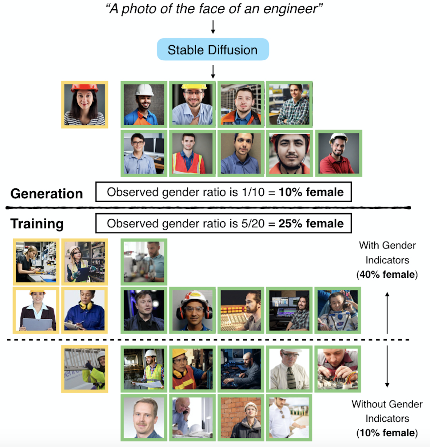
Figure 1: Comparing generated and training images for engineer, the model clearly seems to amplify bias by going from 25% to 10% female in training vs. generated images. However, when looking at the subset of training examples without gender indicators in captions (similar to our prompts), the model does not amplify bias.

Imagine that a model generates images of engineers that are female 10% of the time. When examining the training data, we may assume that models reflect associations in the data and expect to observe roughly 10% female as well. However, it would be problematic for a model to instead exacerbate existing imbalances by generating engineer images that are only 10% female, while the training engineer images are 25% female, as shown in Figure 1. This phenomenon, known as bias amplification Zhao et al. (2017), is concerning because it further reinforces stereotypes and widens disparities. While previous works suggest that models amplify biases (Zhao et al., 2017; Wang et al., 2018; Hall et al., 2022; Hirota et al., 2022; Friedrich et al., 2023), there remain unanswered questions about the paradoxical nature of bias amplification: Given that models learn to fit the training data, why do models intensify biases found in the data as opposed to strictly representing them?

In this paper, we investigate how model biases compare with biases found in the training data. We focus on the text-to-image domain and analyze gender-occupation biases in Stable Diffusion, (Rombach et al., 2022) as well as its publicly available training dataset LAION (Schuhmann et al., 2022), which consists of image-caption pairs in English (§2). To select training examples, we identify captions that mention an occupation (e.g., engineer) and obtain corresponding images. We follow previous work (Bianchi et al., 2023; Luccioni et al., 2023) and use prompts that contain a given occupation (e.g., “A photo of the face of an engineer”) to generate images. For each occupation, we then classify binary gender to measure bias in corresponding training and generated images, and compare the respective quantities to determine whether the model amplifies biases from its training data (§3).

At first glance, it appears that the model amplifies bias considerably (12.57%) using existing approaches (§4). However, we discover clear distributional differences when comparing how training captions and prompts are written, which impact amplification measurements. For example, an inherent distinction is that captions often contain explicit gender information while prompts used to study gender-occupation biases do not. As shown in Figure 1, the gender distribution for captions with gender indicators (40% female) clearly differs from the distribution for captions without such indicators (10% female) for the occupation engineer.

Instead of naively considering all training captions that contain a given occupation when analyzing bias amplification, we propose focusing on subsets of the training data that reduce distribution shifts between training and generation (§5). We introduce two approaches to account for distributional differences observed in qualitative evaluation: (1) Excluding captions with explicit gender information and (2) Using nearest neighbors (NN) on text embeddings to select training captions that closely resemble prompts. Both approaches restrict the search space of training texts to more closely match prompts, which results in considerably lower amplification measures. We then eliminate differences between training captions and prompts by utilizing the captions themselves to generate images (§6), and show that amplification is minimal. By modifying either the captions or prompts used to evaluate amplification, we provide insights into how the subsets of data used to measure bias at training and generation impact amplification.

To summarize, we study gender-occupation bias amplification in Stable Diffusion and highlight notable discrepancies between texts used for training and generation. We demonstrate that naively quantifying bias provides an incomplete and misleading depiction of model behavior. Our work emphasizes that comparisons of dataset and model biases should factor in distributional differences and evaluate comparable distributions. We hope that our work encourages future studies that analyze model behavior through the lens of the data.

2 Experimental Setup

2.1 Dataset and Models

To study bias amplification, we use Stable Diffusion (Rombach et al., 2022), a text-to-image model that generates images based on a textual description (prompt). Stable Diffusion is trained on pairs of captions and images taken from LAION-5B (Schuhmann et al., 2022), a public dataset created by scraping images and their captions from the web. We focus on two versions, Stable Diffusion 1.4 and 1.5, which are both trained on text-image pairs from the 2.3 billion English portion of LAION-5B.

2.2 Gender Classification

We analyze bias in images with respect to perceived gender. To classify binary gender at scale, we utilize an automated approach. Therefore, it is important to verify that images include faces, and that perceived gender is discernible from these images. We first check whether an image contains a single face using a face detector. Then, we use CLIP (Radford et al., 2021), a multimodal model with zero-shot image classification capabilities, to predict gender (note that Stable Diffusion also uses CLIP’s text encoder to encode prompts). To exclude cases where gender is difficult to infer (e.g., faces might be blurred or obscured), we only consider images for which the predicted gender probability is greater than or equal to 0.9. We apply these filtering steps to training and generated images.

2.3 Occupations

Similar to previous works, we analyze gender-occupation biases for occupations that exhibit varying levels of bias (Rudinger et al., 2018; Zhao et al., 2018; De-Arteaga et al., 2019). These include occupations that skew male (e.g., CEO, engineer), fairly balanced (e.g., attorney, journalist), and female (e.g., dietitian, receptionist) based on the training data. In total, we consider 62 job occupations, which can be found in Table 4 in the Appendix.

3 Methodology

#	Prompt
1	A photo of the face of a/an [OCCUPATION]
2	A portrait photo of a/an [OCCUPATION]
3	A photo of a/an [OCCUPATION] smiling
4	A photo of a/an [OCCUPATION] at work

Table 1: The four prompts we use to generate images. “[OCCUPATION]” is a placeholder we replace with one of the 62 occupations we use.

3.1 Measuring Model Bias

To measure biases exhibited by the model, we generate images using four prompts, shown in Table 1. These prompts deliberately do not contain gender information since we want to capture biases learned by the model. Both prompts #1 and #2 also direct the model to generate faces by including “face”/“portrait”. We generate 500 images per occupation and prompt using various random seeds (which is used to generate random noise). We define $G_{P_{o}}$ as the percentage of females in generated images for a prompt $P$ describing an occupation $o$.

3.2 Measuring Data Bias

Given that the training data consists of image-caption pairs, we use captions to obtain relevant training examples. In doing so, we assume that the training captions relating to a given occupation mention the occupation. We use the search capabilities of WIMBD (Elazar et al., 2023), a tool that enables exploration of large text corpora, to query LAION. We define $T_{S_{o}}$ as the percentage of females in images for a training subset $S$ corresponding to occupation $o$ (we provide more details on example selection in Section 4).

3.3 Evaluating Bias Amplification

We compute bias amplification by comparing the percentage female in generated ($G_{P_{o}}$) vs. training ($T_{S_{o}}$) images for a specific occupation $o$ using the approach outlined in Zhao et al. (2017):

$$A_{P_{o},S_{o}}=|G_{P_{o}}-50|-|T_{S_{o}}-50|$$

This formulation takes into account that amplification for a given occupation is specific to the prompt $P_{o}$ used to generate images, as well as the chosen subset of training examples $S_{o}$. For a set of occupations $O$, the expected amplification is:

$$\mathop{\mathbb{E}}_{o\in O}[A_{P_{o},S_{o}}]=\frac{1}{|O|}\sum_{o\in O}A_{P_{o},S_{o}}$$

$A_{P_{o},S_{o}}$ is calculated for each occupation and aggregated across occupations ($O$) to obtain $\mathbb{E}[A_{P_{o},S_{o}}]$ for each prompt. We then average $\mathbb{E}[A_{P_{o},S_{o}}]$ across all four prompts. For occupations that skew male in the training data, bias is amplified if it skews further male in generated images, and vice versa for occupations that skew female. Bias decreasing from training to generation is considered de-amplification. We exclude occupations that exhibit different directions of bias at training and generation from our analysis.

Caption	Details
Portrait of smiling young female mechanic inspecting a CV joint on a car in an auto repair shop	Contains person description (smiling young female), activity, and location
Muscular bearded athlete drinks water after good workout session in city park	Contains person description (muscular bearded), clues about attire (workout clothes), and activity
Portrait of a salesperson standing in front of electrical wire spool with arms crossed in hardware store	Contains activity, information about surroundings, and location

Table 2: Training captions often include additional context and details (e.g., descriptions, activity information) that reduce ambiguity. As shown in these examples, captions may contain explicit and implicit gender information. In contrast, the prompts we use to generate images (Table 1), lack specificity and convey limited information.

4 Naive Approach

We examine the extent to which Stable Diffusion amplifies gender-occupation biases from the data by selecting training examples that contain a given occupation in the caption (e.g., all captions that contain the word “president”). In practice, we randomly sample a subset of 500 training examples as opposed to using all examples. We find that Stable Diffusion amplifies bias relative to the training data by 12.57% on average across all occupations and prompts (10.24% for Prompt #1, as shown in Figure 2). This behavior is concerning because instead of reflecting the training data and its statistics, the model compounds bias by further underrepresenting groups. However, when qualitatively inspecting examples, we observe discrepancies in how occupations are presented in captions vs. prompts due to varying levels of ambiguity.

For example, we notice the use of explicit gender indicators to emphasize deviations from stereotypical gender-occupation associations, such as female mechanics. While gender information is used frequently in captions, we hypothesize that usage is more common for underrepresented groups. If this hypothesis holds, the gender distribution would shift closer towards balanced in resulting training images. As a result, the decision to focus on all captions vs. captions without any gender indicators might exaggerate amplification measures.

More generally, prompts commonly used to study gender-occupation bias are intentionally underspecified, or lack detail. Underspecification results in the model having to generate images from textual inputs that are vague and open to interpretation (Hutchinson et al., 2022; Mehrabi et al., 2023). For instance, the prompt “A photo of the face of a/an [OCCUPATION]” does not contain any adjectives or information about surroundings, activities, etc. In contrast, captions may contain context and details that result in less ambiguous descriptions, as shown in Table 2.

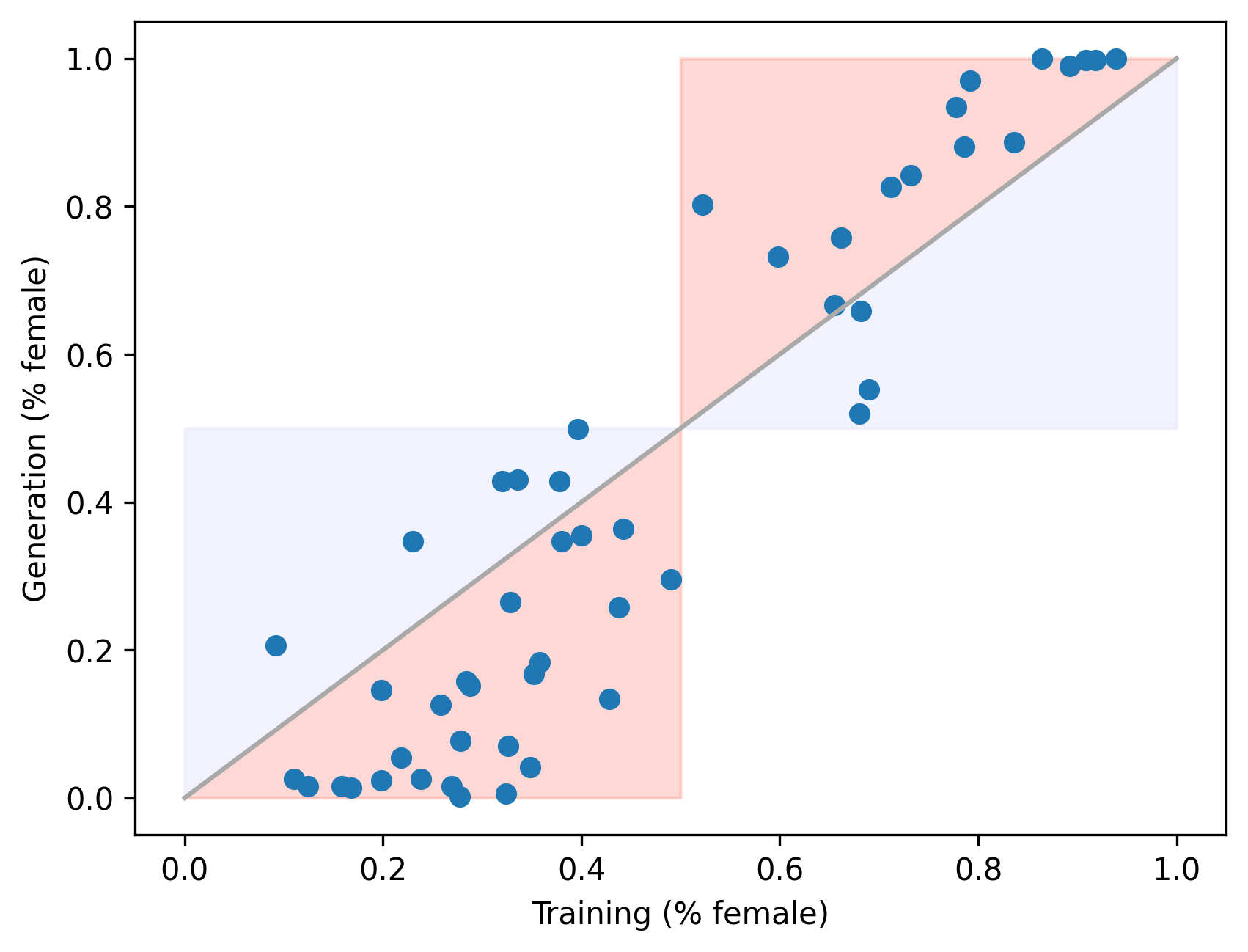
Figure 2: Bias amplification for our initial naive approach. There appears to be consistent bias amplification between training and generation. The x-axis corresponds to the % female in training images, and the y-axis corresponds to the % female in generated images (using Prompt #1). Each point represents an occupation. Shading: Amplification and De-Amplification.

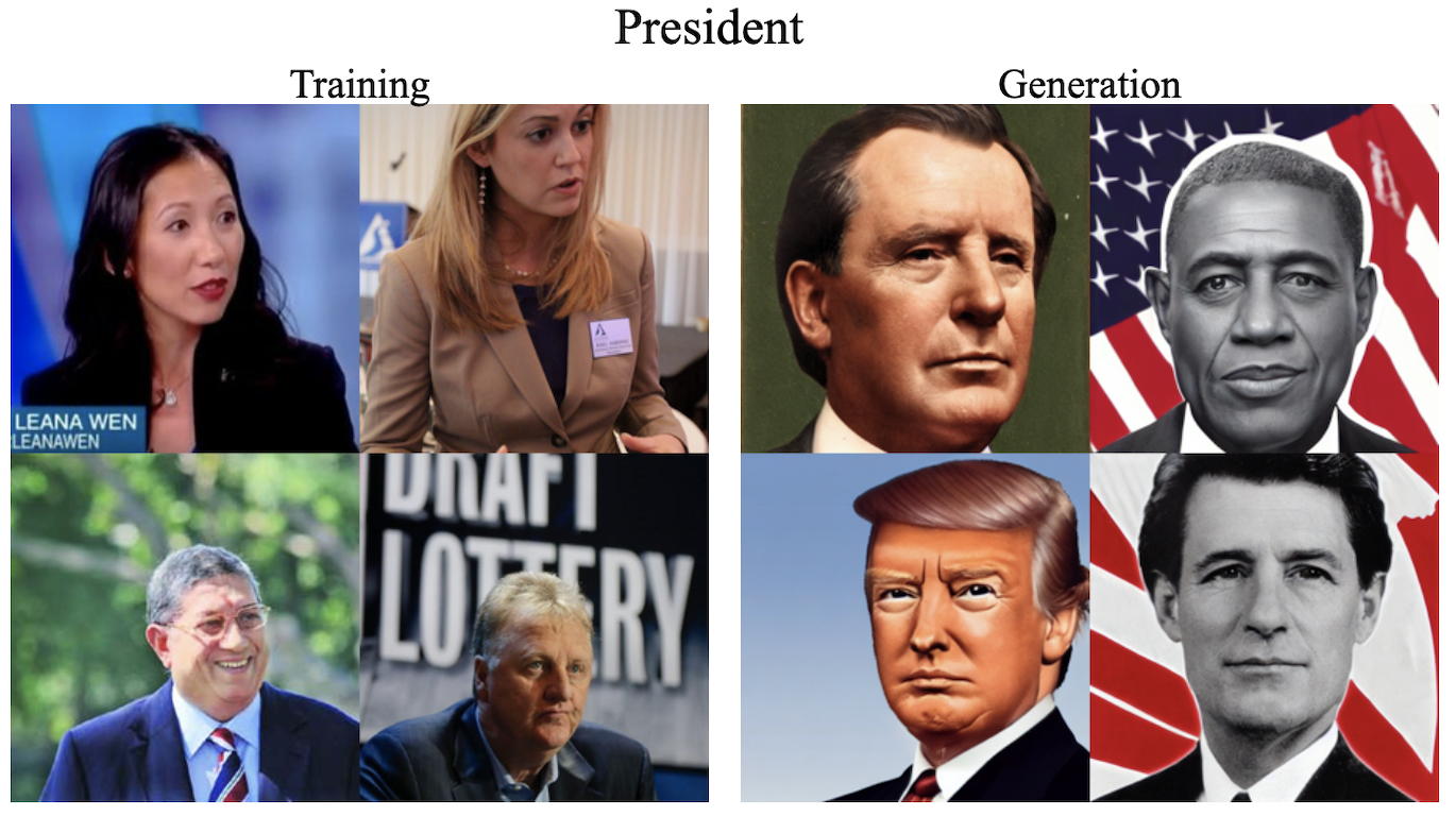
(a) Training captions for President: 1) "Leana Wen, Planned Parenthood president…" 2) "New Schaumburg Business Association President…" 3) "BCCI president N Srinivasan…" 4) "Indiana Pacers president of basketball operations…"

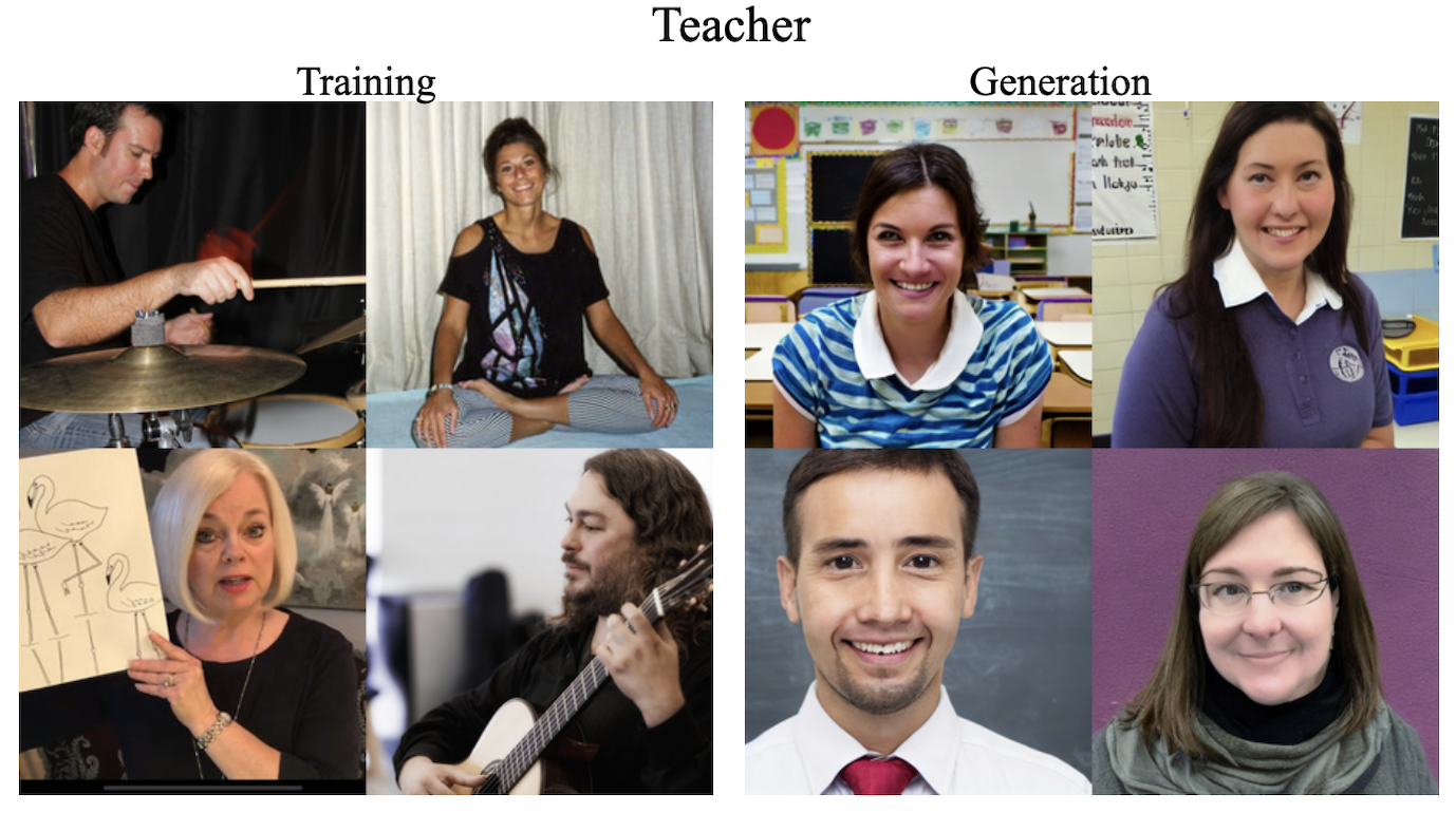
(b) Training captions for Teacher: 1) "Brad Draper, percussion teacher…" 2) "teacher/author in the 80s sits in yoga lotus pose…" 3) "Jo Anne Young Art Teacher…" 4) "patrick oconnell Classical Guitar Teacher…"

Figure 3: We handpick examples of discrepancies in how occupations are depicted in training vs. generated examples for President (left) and Teacher (right) professions using our naive approach.

Discrepancies in how captions and prompts are written also impact how occupations are depicted in training and generated images. These differences are especially notable for occupations that have multiple interpretations. For example, when querying for training examples containing “president”, the resulting captions may refer to various types of presidents, including the president of a company or organization, as shown in Figure 3(a). However, when generating images using the prompt “A photo of the face of a president”, the model appears to interpret president as a leader of a country, often the United States (we also showcase similar differences for the occupation teacher in Figure 3(b)).

To make reasonable comparisons between bias at training vs. generation, we should compare gender ratios over similar captions and prompts. Therefore, we cannot conclude whether differences in gender ratios between training and generation are due solely to the model amplifying bias, or other confounding factors that contribute to amplification. Next, we focus on reducing the impact of distribution shifts on bias amplification evaluation.

5 Reducing Discrepancies

In this section, we evaluate approaches to reduce training and generation discrepancies by restricting the search space of training examples. Note that prompts $P_{o}$ remain fixed, while the subset of training examples $S_{o}$ varies in our analysis.

5.1 Captions Without Explicit Gender Indicators

A notable distinction between training and generation is the use of explicit gender indicators, which is absent from prompts. On average, more than half the captions (59.5%) contain explicit gender information. Furthermore, gender usage in captions varies depending on which gender is underrepresented for a given occupation. For example, images of female mechanics in the training data frequently accompany captions that indicate the mechanic is female. In comparison, this specification is less common for male mechanics (only 30% of male mechanic examples contain explicit gender indicators, as opposed to 68% for female mechanics).

To validate these observations, we compute the correlation between the percentage of females in training images and the percentage of captions with female indicators. We expect that female-skewing occupations are less likely to contain explicit female gender indicators in captions, resulting in a negative correlation. The Pearson’s correlation coefficient is indeed negative, with a coefficient value of -0.458 and statistically significant (significance level $<0.05$). These results suggest that including training examples with gender information during evaluation may exaggerate amplification.

Addressing Gender Indicators

To assess whether amplification differs for the subset of captions without indicators, we split the training examples selected in Section 4 by detecting direct gender mentions in the captions (more details in A.3). We focus on the subset of captions, $S_{o}$, without explicit male or female indicators.

Reduced Bias Amplification

We observe that bias amplification is noticeably lower when focusing on the no-gender indicator subset of training examples. Compared to the initial amplification of 12.57% for keyword querying, the average amplification for captions without gender indicators is 8.66% ($\downarrow$ 31%), as shown in Table 3. This behavior aligns with the reasoning described above — gender indicators are more likely to delineate the presence of the underrepresented gender, which in turn inflates amplification measures.

5.2 Nearest Neighbors (NN)

Beyond explicit gender indicators, there are clear differences in the information conveyed by prompts vs. captions. The prompts we use are concise and structured, but lack concrete details. On the other hand, randomly sampled training captions are more diverse and vary in their usage of the occupation and the amount of contextual information, as highlighted in Table 2 and Figure 3. Furthermore, captions may contain implicit gender information (e.g., descriptors, attire, activity details) which is absent from prompts.

These qualitative differences are also apparent when comparing caption and prompt text embeddings. We use Sentence-BERT (Reimers and Gurevych, 2019) to compute text embeddings, and calculate the average pairwise cosine similarity between caption and prompt embeddings for each occupation. We find that the average cosine similarity across occupations is 0.385, indicating that captions and prompts are highly dissimilar (relative to nearest neighbors, which we will see next).

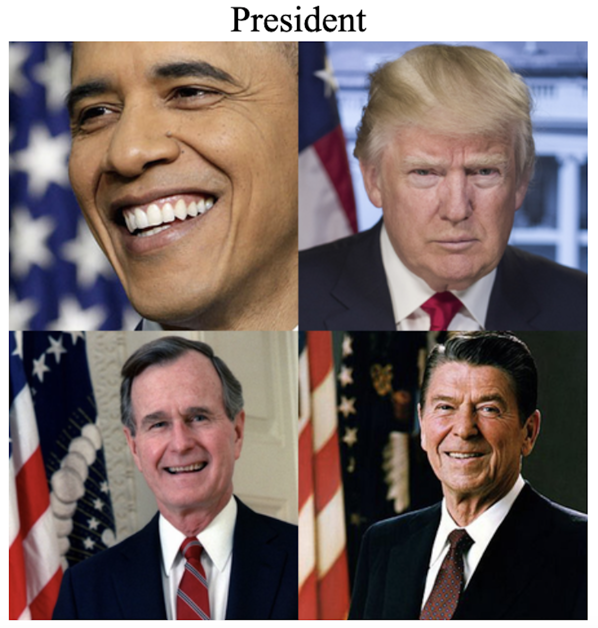
(a) Training captions for President: 1) "The president is pictured smiling." 2) "President Donald J. Trump - Official Photo" 3) "Portrait of President George H. W. Bush" 4) "Official Portrait of President Ronald Reagan"

(b) Training captions for Teacher: 1) "Picture of a teacher in the classroom" 2) "Portrait of a smiling teacher in a classroom." 3) "Portrait of teacher woman working" 4) "Teacher smiling in classroom, portrait"

Figure 4: Training examples chosen with Nearest Neighbors. Selected training captions and images are more similar to prompts and generated images.

Approach	Model	Prompt #1	Prompt #2	Prompt #3	Prompt #4	Average
Naive Approach	SD 1.4	10.24	17.57	10.77	11.68	12.57
	SD 1.5	10.87	16.36	11.15	9.91	12.07
No Gender Indicators	SD 1.4	6.49	13.58	7.09	7.49	8.66
	SD 1.5	6.76	12.41	6.82	5.87	7.97
Nearest Neighbors	SD 1.4	3.59	12.62	5.58	5.27	6.76
	SD 1.5	4.01	11.14	5.21	3.65	6.01
Nearest Neighbors +	SD 1.4	1.11	8.72	3.06	4.05	4.35
No Gender Indicators	SD 1.5	1.55	7.29	2.78	2.72	3.59

Table 3: Bias Amplification across occupations using Stable Diffuson (SD) 1.4 and 1.5, for each prompt and averaged across prompts. Amplification lowers considerably when using nearest neighbors to select training captions and excluding captions with gender indicators. We see further reductions when combining approaches.

Addressing Similarity Discrepancies

To account for these gaps, we propose using nearest neighbors (NN) to select captions that closely resemble prompts. We can find NN by considering all captions that contain a given occupation, and selecting examples based on the similarity between caption and prompt text embeddings instead of sampling randomly. As a result, the chosen captions are closer in structure and wording to prompts. We use Sentence-BERT to obtain text embeddings and compute the cosine similarity between embeddings to measure the similarity between captions and prompts. For a given occupation, we consider the top-$k$ similar captions, where $k=500$.

Applying NN, the average cosine similarity between caption and prompt embeddings increases to 0.704 ($\uparrow$ 83% from keyword querying), which occurs by design since we directly target examples that resemble prompts. Note however, that the increase in similarity is also reflected in image embeddings. The pairwise similarity of CLIP image embeddings increases with NN ($\uparrow$ 13% from keyword querying), indicating that chosen training and generated images are slightly more similar.

There are noticeable qualitative improvements as well. NN chooses captions that are closer in structure and meaning to prompts (e.g., “Picture of a teacher in the classroom”), which also impacts corresponding training images. As shown in Figure 4, the training images corresponding to NN captions for the word “president” primarily represent world leaders (often US presidents), while captions for the word “teacher” depict educators in classroom settings.

Reduced Bias Amplification

When selecting training examples $S_{o}$ using NN, we see that bias amplification reduces considerably across occupations and prompts, as shown in Table 3. The average amplification drops to 6.76% ($\downarrow$ 46% relative to keyword querying). While NN yields increased similarity between training and generated examples, there are still unresolved sources of distribution shift that impact amplification measures.

5.3 Combining Approaches

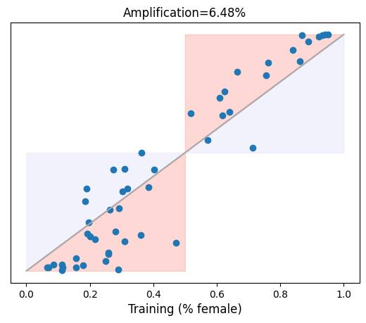
(a) Captions without Gender Indicators

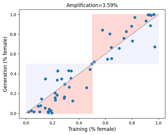
(b) Nearest Neighbors

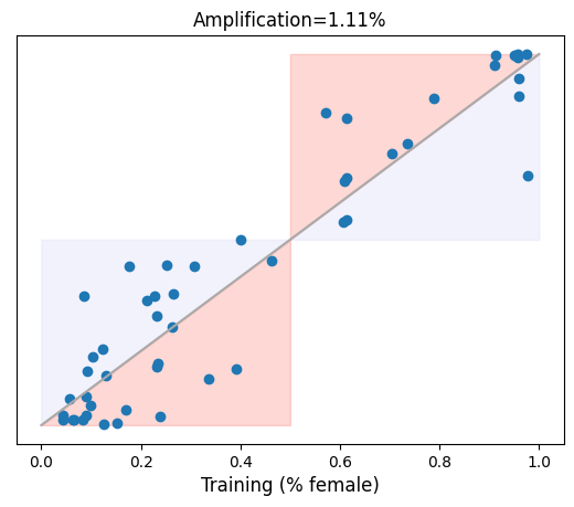
(c) Combined Approach

Figure 7: Bias amplification for various approaches to address discrepancies between training and generation. The proposed approaches yield lower bias amplification, especially the combined method (c). Results are shown for Prompt #1. Regions are shaded based on Amplification and De-Amplification.

We observe that amplification further reduces when combining the no-gender indicator subset with NN, as shown in the last rows in Table 3. The average amplification decreases to 4.35%, which is noticeably lower compared to the values for each method individually. Both methods work in tandem to reduce distributional differences in complementary ways, perhaps by targeting both explicit and implicit gender information. We also observe greater reductions for specific prompts; as shown in Figure 7(c), amplification is just 1.11% for Prompt #1.

We perform a one-sample t-test to test the null hypothesis that the expected amplification is 0 for each of the prompts; we fail to reject the null hypothesis for prompts #1 and #3 and reject the null hypothesis for prompts #2 and #4 (significance level $<0.05$). Our results indicate a portion of amplification is unexplained for all prompts, especially prompts #2 and #4, and may involve more subtle confounding factors. Although the proposed methods do not account for all possible discrepancies between training and generation, we observe that the bias measures become closer as we select subsets of training captions that resemble prompts.

6 Removing Distributional Differences: A Lower Bound

While the previous approaches reduce discrepancies between training and generation by evaluating amplification with captions that are more similar to prompts, we can instead modify the prompts we use to align with captions more closely. In this setup, we use the original training subset ($S_{o}$) from Section 4, but the prompts ($P_{o}$) now match the captions verbatim. For every prompt in $P_{o}$, we generate 10 images, and then compute amplification using $P_{o}:=S_{o}$ for each occupation.

By design, this approach removes mismatches between captions and prompts, since prompts and captions are now identical. We then ask: Does using identical texts to measure training and generation bias lower amplification? We hypothesize that enforcing prompts and captions to match yields similar bias measurements, which in turn reduces amplification. As shown in Figure 5(a), amplification is minimal when $P_{o}=S_{o}$ and most occupations reside along the diagonal (no amplification). The average amplification drops to 0.68%, indicating that the model mostly reflects training bias. Furthermore, amplification remains consistently low, even for occupations that are highly imbalanced.

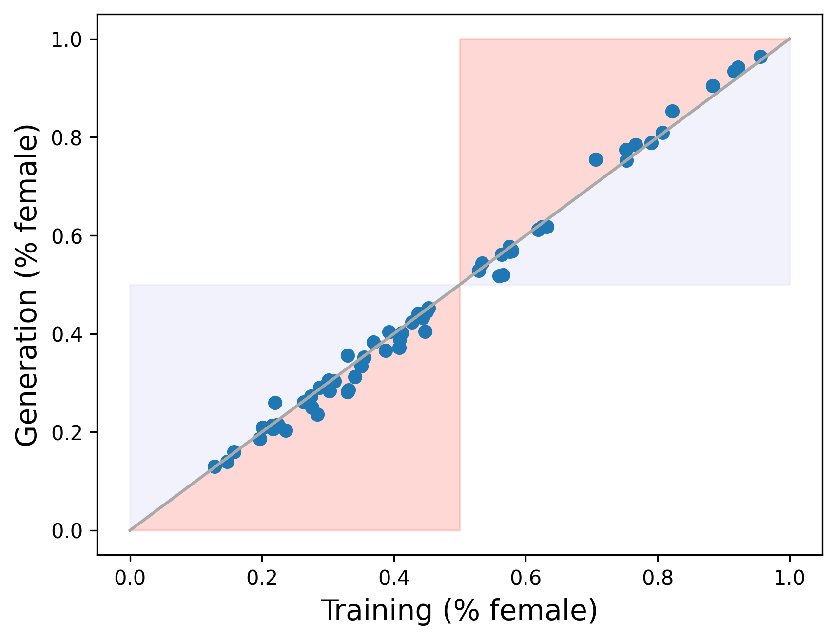
(a) All Captions

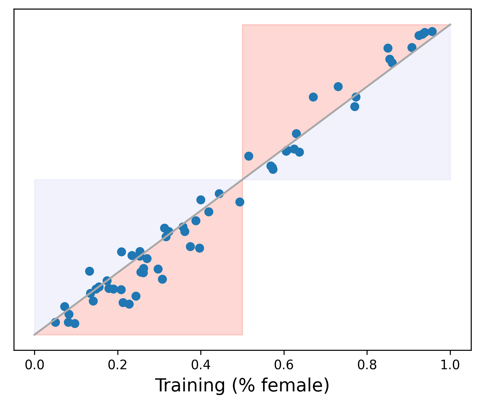
(b) Captions without Gender Indicators

Figure 5: Bias amplification when prompting with training captions. We observe minimal amplification when $P_{o}=S_{o}$ (left). This behavior mostly holds when focusing on captions without explicit gender indicators (right). Shading: Amplification and De-Amplification.

For captions that contain either male or female gender indicators, the model generates images that match the gender of corresponding training images (with 98.41% accuracy), since this information is directly provided in the prompt. Therefore, we analyze results separately on the subset of captions without gender indicators. As shown in Figure 5(b), bias amplification is larger for the no gender indicator subset as compared to all captions. That being said, the average amplification remains low at 2.05% ($\downarrow$ 84% relative to keyword querying).13

Although practitioners are unlikely to utilize prompts that exactly match training captions (nor do we make this recommendation), this experiment highlights the impact of distributional similarity between captions and prompts when comparing biases. In addition, it provides a lower bound to the bias amplification problem. In summary, we conclude that the model nearly mimics biases from the data when prompted with training captions.

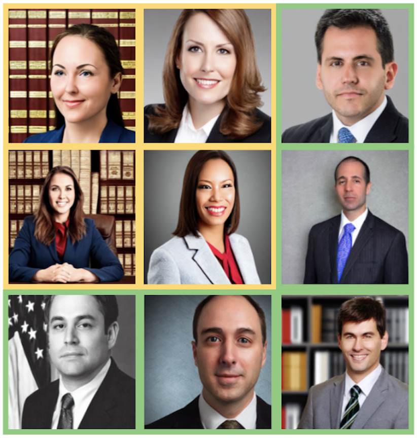
(a) A photo of the face of an attorney

(b) A portrait photo of an attorney

(c) A photo of an attorney smiling

(d) A photo of an attorney at work

Figure 6: Generated examples for the occupation attorney using different prompts. Specific wording and phrasing choices in prompts lead to noticeable differences in the % of generated images that are female (boxes are colored based on predicted female and predicted male). Although we only include 9 images per prompt here, these proportions are similar to what is exhibited in the 500 generated images.

7 Related Work

Relating pretraining data to model behavior

There is a growing body of work focused on studying pretraining data properties and statistics, as well as understanding their relation to model behavior. This type of large-scale data and model analysis provides useful insights into model learning and generalization capabilities (Carlini et al., 2023). Recent work shows that few-shot capabilities of large language models are highly correlated with pretraining term frequencies, and that models struggle to learn long-tail knowledge (Kandpal et al., 2023; Razeghi et al., 2022). Several works have also explored the relationship between pretraining data and model performance from a causal perspective (Biderman et al., 2023; Elazar et al., 2022; Longpre et al., 2023). For example, Longpre et al. (2023) comprehensively investigate how various data curation choices and pretraining data slices affect downstream task performance.

Bias Amplification

Our work is strongly inspired by the findings of Zhao et al. (2017), who show that structured prediction models amplify biases present in the data. However, there are important differences to note. First, their task involves jointly predicting multiple target labels, including gender, as opposed to generating images. Additionally, their work focuses on mitigating amplification, as opposed to investigating various factors that contribute to amplification. Hall et al. (2022) consider how data, training, and model-related choices influence amplification using a classification setup with synthetic bias, but do not examine how distribution shifts contribute to amplification.

Friedrich et al. (2023) also compare biases exhibited by LAION and Stable Diffusion, and show that the model displays bias amplification. Instead of identifying relevant training examples using captions, they use text-image similarity between prompts and training images. Similar to Zhao et al. (2017), their work mainly focuses on mitigating model bias using their proposed method, fair diffusion, while our work is centered around analyzing confounding factors that impact amplification.

Bias in text-to-image models

While it is well-established that language and vision models are susceptible to biases individually, recent work has shown that text-to-image models are prone to similar biases. Several works analyze various biases in text-to-image models, including underexplored topics such as geographical disparities (Basu et al., 2023; Naik and Nushi, 2023) and intersectional biases (Fraser et al., 2023; Luccioni et al., 2023). Bianchi et al. (2023) demonstrate that stereotypes persist even after prompting the model with counter-stereotypes. However, these works primarily focus on evaluating model biases, and do not examine the training data.

8 Discussion

Generalizability

Our work demonstrates that using naive procedures to evaluate bias amplification can lead to exaggerated amplification measures. While our analysis does not account for all sources of distribution shift that contribute to amplification, it is meant to be illustrative. We encourage future studies to build on our findings by examining different experimental setups (i.e., datasets, models, and types of bias) to gain a more comprehensive understanding of bias amplification and the impact of confounding factors.

Variation Across Prompts

As we highlight in Figure 6, small changes to prompts can have a resounding effect on conclusions about model bias. For example, “A portrait photo of an attorney” skews heavily male while “A photo of an attorney at work” skews female in generated images. Furthermore, reductions in amplification differ based on the prompt (e.g., Prompt #1 exhibits an 89% reduction as opposed to 49% for Prompt 2), indicating that the confounding factors have a varying impact. These results suggest that there may also be prompt-specific sources of distribution shift, which is an important consideration when choosing prompts.

Amplification Baseline

Our interpretation of bias amplification is centered around models exacerbating biases found in the training data as opposed to real-world statistics (Kirk et al., 2021; Bianchi et al., 2023). Both approaches are useful to study but answer fundamentally different questions. Our approach offers insights into whether model behavior reflects the training data, while real-world amplification captures how well the data and model together reflect reality.

Connection to Simpson’s Paradox

The title of our paper alludes to Simpson’s Paradox (Simpson, 1951), a phenomenon in which a trend or relationship observed in subgroups within the data reverses or disappears when subgroups are combined. We draw direct parallels to our analysis and insights; although we observe substantial amplification in our initial setup, amplification reduces drastically after selecting specific subsets of the training data and decreasing the impact of confounding factors.

Recommendations

Our findings underscore how distribution shifts contribute to bias amplification, which has important implications. Those involved in data-focused efforts should consider how practitioners specify prompts and interact with models when curating training data. Alternatively, crowdsourcing or automatically rewriting existing training captions to reflect real-world model usage may result in lower amplification. Additionally, we recommend that evaluations use multiple prompts and remove prompt-specific confounding factors (e.g., by using NN to select relevant training examples).

9 Conclusion

In summary, we investigate whether Stable Diffusion amplifies gender-occupation biases by comparing training data and model biases. We highlight how naive evaluations of amplification fail to consider distributional differences between training and generation, which leads to a misleading understanding of model behavior. Although amplification is not eliminated entirely, we observe that reducing discrepancies between captions and prompts during evaluation results in substantially lower measurements. We strongly recommend that any analysis comparing training data and model biases, or any dataset and model properties more generally, account for various distribution shifts that skew evaluations.

Limitations

Beyond the training data, another source of bias is the text embeddings obtained from CLIP. By solely comparing biases in the data vs. those exhibited by Stable Diffusion, our analysis overlooks biases that arise from encoding prompts. As a result, we cannot disentangle how much this component impacts overall amplification. Note that the effect of such an external embedding cannot be easily accounted for, since CLIP’s training data is not public. More work is needed to understand the impact of using external, frozen models as a model component.

Additionally, we automate gender classification using CLIP because previous works have shown that CLIP gender predictions align with human annotations and CLIP gender classification performance on the FairFace dataset is strong ($>95\%$) across various racial categories. Nevertheless, we recognize the limitations of using a model to classify gender in images, since CLIP inherits biases from its training data.

Ethics Statement

Scope of Work

Our work centers around critically examining bias amplification evaluation. The approaches we propose to reduce distribution shifts observed during evaluation do not solve underlying gaps between the data used to train models and how users interact with models. Rather, they serve to deepen our understanding of why models amplify biases present in the training data. Ideally, our findings will motivate future work on 1) thorough and nuanced evaluations of bias amplification and 2) fundamentally addressing training and generation discrepancies from a data perspective.

Bias Definition

Our work focuses on a narrow slice of social bias analysis by studying gender-occupation stereotypes. However, since models exhibit various types of discriminatory bias (e.g., racial, age, geographical, socioeconomic, disability, etc.), as well as intersectional biases, it is equally important to perform evaluations for these definitions of bias. Furthermore, we only consider binary gender, which has clear drawbacks. Our analysis ignores how text-to-image models perpetuate biases for non-binary identities and relies on information such as appearance and facial features to infer gender in training and generated images, which can further propagate gender stereotypes.

Geographical Diversity

The captions and prompts used to study bias are solely written in English. We hope future work will shed light on multilingual bias amplification in text-to-image models. It is also worth noting that the gender-guesser library (infers gender from names) likely performs worse on non-Western names. The documentation mentions that the library supports over 40,000 names and covers a “vast majority of first names in all European countries and in some overseas countries (e.g., China, India, Japan, USA)”. Therefore, the name coverage (or lack thereof) impacts our ability to identify captions with gender information.

		Occupations
accountant	dentist	journalist	poet	singer
architect	dietitian	lawyer	politician	student
assistant	doctor	librarian	president	supervisor
athlete	engineer	manager	prime minister	surgeon
attorney	entrepreneur	mechanic	professor	teacher
author	fashion designer	musician	programmer	technician
baker	filmmaker	nurse	psychologist	therapist
bartender	firefighter	nutritionist	receptionist	tutor
ceo	graphic designer	painter	reporter	veterinarian
chef	hairdresser	pharmacist	researcher	writer
comedian	housekeeper	photographer	salesperson
cook	intern	physician	scientist
dancer	janitor	pilot	senator

Table 4: List of 62 occupations used to study gender-occupation biases.

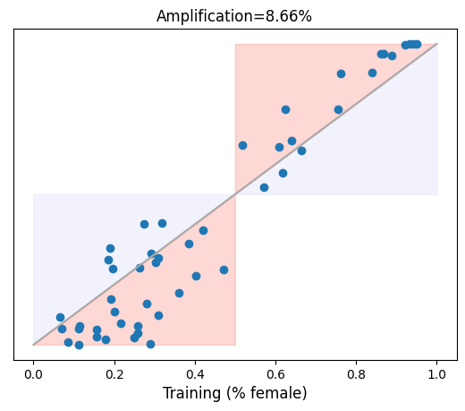
(a) Captions without Gender Indicators

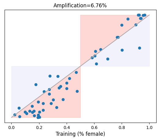
(b) Nearest Neighbors

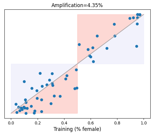
(c) Combined Approach

Figure 8: Bias amplification for various approaches to address discrepancies between training and generation. The proposed approaches yield lower bias amplification, especially the combined method (c). Results are averaged across all prompts. Regions are shaded based on Amplification and De-Amplification.

Appendix A Appendix

A.1 List of Occupations

A full list of occupations is shown in Table 4.

We exclude occupations that exhibit different directions of bias at training and generation from our amplification results, since this behavior does not adhere to our definition of amplification. There are 5 occupations (assistant, author, dentist, painter, supervisor) that exhibit switching behavior consistently for all prompts, using both SD 1.4 and 1.5. More research is needed to understand and explain this behavior.

A.2 Image Gender Classification

While CLIP is susceptible to biases (Hall et al., 2023), its gender predictions have been shown to align with human-annotated gender labels (Bansal et al., 2022; Cho et al., 2022). In addition, we perform human evaluation with 7 participants on 200 randomly selected training and generated images. We ask participants to provide binary gender annotations (or indicate that they are unsure), and find that Krippendorff’s coefficient, which measures inter-annotator agreement, is high ($\alpha=0.948$). Additionally, 98% of CLIP predictions match the majority vote annotations.

A.3 Explicit Gender Indicators

To identify captions with explicit gender information, we consider 1) gender words (male, female, man, woman, gent, gentleman, lady, boy, girl), 2) binary gender pronouns (he, him, his, himself, she, her, hers, herself), and 3) names. We perform named entity recognition using the en_core_web_lg model from spaCy to identify name mentions, and then use the gender-guesser library https://pypi.org/project/gender-guesser/ to infer gender.

Occupation	Training	Prompt 1	Prompt 2	Prompt 3	Prompt 4	SD (Prompts)
accountant	29.8	29.5	3.4	43.8	35.7	15.1
architect	31.4	4.2	2.2	3.0	0.0	1.5
assistant	44.6	67.1	56.3	71.9	75.6	7.3
athlete	44.8	80.0	51.9	69.3	77.3	11.0
attorney	29.2	42.8	9.4	43.1	65.1	19.9
author	42.8	83.6	53.0	81.5	61.0	13.1
baker	41.4	81.1	31.2	58.8	59.3	17.7
bartender	36.8	16.8	2.6	12.9	22.9	7.4
ceo	15.0	2.6	1.8	4.8	11.9	4.0
chef	28.0	7.0	1.2	1.4	5.8	2.6
comedian	21.8	2.4	0.0	3.6	1.0	1.4
cook	35.0	34.7	8.6	49.4	69.3	22.2
dancer	81.0	88.7	98.8	99.0	100.0	4.6
dentist	58.6	41.4	4.4	29.2	41.8	15.2
dietitian	95.2	100.0	100.0	100.0	99.8	0.1
doctor	40.8	33.7	3.8	14.6	57.6	20.5
engineer	20.6	2.6	0.2	1.2	0.0	1.0
entrepreneur	43.6	42.8	1.8	12.8	34.6	16.4
fashion_designer	76.0	93.4	80.8	89.8	97.2	6.1
filmmaker	29.2	12.6	3.2	8.3	14.9	4.5
firefighter	14.6	1.6	1.0	15.9	3.2	6.1
graphic_designer	52.8	11.8	14.4	32.7	41.6	12.5
hairdresser	79.2	97.0	95.6	94.6	97.6	1.2
housekeeper	91.4	99.0	99.8	100.0	100.0	0.4
intern	57.6	65.8	31.5	77.2	53.4	17.0
janitor	20.4	1.6	3.0	14.6	5.7	5.0
journalist	38.4	49.9	59.9	68.8	64.0	7.0
lawyer	27.6	26.5	8.0	39.0	47.7	14.9
librarian	74.4	88.1	83.6	93.6	94.8	4.5
manager	13.0	20.6	7.8	29.7	42.8	12.8
mechanic	17.6	1.6	0.0	0.2	35.3	15.0
musician	22.6	5.4	4.2	7.2	3.2	1.5
nurse	88.8	100.0	100.0	100.0	100.0	0.0
nutritionist	83.6	99.8	92.8	96.6	97.5	2.5
painter	52.6	36.4	12.2	17.6	3.6	12.0
pharmacist	68.0	84.2	26.9	54.9	91.7	25.6
photographer	55.0	52.0	27.5	46.5	13.2	15.4
physician	39.4	35.5	2.0	37.5	59.3	20.5
pilot	30.4	34.7	12.2	66.3	15.9	21.4
poet	30.8	15.2	2.0	19.5	32.8	11.0
politician	21.6	14.5	4.2	15.9	9.6	4.6
president	19.6	1.4	0.2	8.0	0.8	3.1
prime_minister	24.0	15.7	10.6	13.2	21.4	4.0
professor	28.2	7.8	2.8	9.2	5.3	2.4
programmer	23.0	0.2	0.0	0.2	0.0	0.1
psychologist	58.6	44.3	21.6	57.2	52.9	13.8
receptionist	91.4	99.8	100.0	99.8	99.8	0.1
reporter	44.4	54.8	55.2	55.1	67.8	5.5
researcher	44.6	80.2	41.8	67.6	50.9	14.8
salesperson	39.8	43.0	5.2	33.1	33.7	14.2
scientist	33.4	25.7	24.0	29.3	23.2	2.4
senator	35.0	13.4	2.0	8.2	5.4	4.2
singer	57.6	73.2	60.3	69.2	60.1	5.7
student	63.0	55.3	48.5	62.1	43.3	7.1
supervisor	65.2	18.3	4.8	16.6	14.9	5.2
surgeon	30.2	82.5	15.6	67.6	82.5	27.5
teacher	63.0	75.8	55.7	94.0	88.0	14.7
technician	31.2	0.6	0.0	0.6	0.0	0.3
therapist	74.8	82.6	63.3	79.2	87.5	9.0
tutor	59.2	48.1	23.1	32.7	43.5	9.7
veterinarian	55.2	66.7	44.7	64.1	89.9	16.0
writer	30.2	73.3	30.1	76.0	63.8	18.3

Table 5: The percentage of females across occupations in training images (using our initial approach from Section 4) and generated images using SD 1.4. We display generation results for each prompt, as well as the standard deviation (SD) across prompts.

Occupation	Training	Prompt 1	Prompt 2	Prompt 3	Prompt 4	SD (Prompts)
accountant	29.8	34.9	5.4	42.1	45.2	15.8
architect	31.4	10.0	2.2	2.2	3.4	3.2
assistant	44.6	69.2	60.8	58.6	77.8	7.6
athlete	44.8	76.6	46.0	50.0	74.3	13.8
attorney	29.2	50.8	11.7	44.3	68.3	20.5
author	42.8	88.2	57.4	75.4	69.0	11.1
baker	41.4	82.3	33.9	53.3	66.6	17.7
bartender	36.8	10.0	2.2	4.8	12.2	4.0
ceo	15.0	1.4	2.0	5.4	18.5	6.9
chef	28.0	12.0	0.8	1.4	7.0	4.6
comedian	21.8	1.6	0.0	1.4	0.6	0.6
cook	35.0	38.4	16.4	43.5	75.1	21.0
dancer	81.0	83.8	97.4	97.6	100.0	6.4
dentist	58.6	41.9	5.4	22.7	20.4	13.0
dietitian	95.2	100.0	100.0	100.0	99.8	0.1
doctor	40.8	38.2	8.8	12.6	53.4	18.4
engineer	20.6	10.6	0.6	1.6	0.0	4.3
entrepreneur	43.6	59.7	4.6	16.9	41.6	21.4
fashion_designer	76.0	97.4	90.3	92.2	98.6	3.5
filmmaker	29.2	18.4	5.2	8.8	7.8	5.0
firefighter	14.6	1.4	0.2	12.5	4.5	4.8
graphic_designer	52.8	22.6	15.3	29.5	63.3	18.4
hairdresser	79.2	99.6	98.0	95.4	97.3	1.5
housekeeper	91.4	99.6	100.0	100.0	100.0	0.2
intern	57.6	72.6	37.1	68.8	60.4	13.8
janitor	20.4	3.6	3.2	8.4	6.2	2.1
journalist	38.4	57.2	60.2	59.7	60.7	1.4
lawyer	27.6	34.1	8.8	36.8	48.2	14.4
librarian	74.4	93.4	85.8	87.8	94.6	3.7
manager	13.0	24.0	14.2	28.7	41.3	9.8
mechanic	17.6	6.4	0.2	1.0	20.8	8.3
musician	22.6	5.4	1.4	2.8	2.8	1.4
nurse	88.8	100.0	100.0	100.0	100.0	0.0
nutritionist	83.6	99.8	97.8	97.2	98.0	1.0
painter	52.6	43.7	20.0	10.6	2.7	15.4
pharmacist	68.0	87.3	26.1	49.6	83.8	25.3
photographer	55.0	58.1	32.5	44.8	26.0	12.3
physician	39.4	46.4	3.2	36.5	62.0	21.6
pilot	30.4	20.9	11.4	35.3	7.5	10.7
poet	30.8	12.4	2.6	11.6	42.1	14.9
politician	21.6	24.9	10.2	16.7	15.7	5.2
president	19.6	4.6	0.4	12.9	2.2	4.8
prime_minister	24.0	25.5	23.0	20.0	42.9	8.9
professor	28.2	9.2	3.0	5.6	8.6	2.5
programmer	23.0	0.8	0.0	1.0	0.0	0.5
psychologist	58.6	51.0	22.4	40.8	52.2	11.9
receptionist	91.4	99.6	100.0	99.2	99.8	0.3
reporter	44.4	53.7	52.5	44.0	57.6	4.9
researcher	44.6	77.3	47.8	52.8	55.0	11.3
salesperson	39.8	56.8	7.0	37.4	30.5	17.8
scientist	33.4	23.0	22.1	15.9	45.3	11.2
senator	35.0	22.7	8.0	12.0	12.5	5.4
singer	57.6	74.0	54.1	66.6	61.2	7.3
student	63.0	44.6	32.3	51.8	40.5	7.0
supervisor	65.2	20.9	5.6	18.2	15.0	5.8
surgeon	30.2	82.0	20.4	50.8	81.6	25.5
teacher	63.0	78.7	58.2	87.4	84.6	11.4
technician	31.2	0.4	0.2	1.6	0.0	0.6
therapist	74.8	88.5	80.8	82.2	88.7	3.6
tutor	59.2	48.8	24.1	24.4	50.4	12.7
veterinarian	55.2	65.6	48.9	48.7	89.5	16.7
writer	30.2	79.2	34.7	69.1	76.6	17.9

Table 6: The percentage of females across occupations in training images (using our initial approach from Section 4) and generated images using SD 1.5. We display generation results for each prompt, as well as the standard deviation (SD) across prompts.

References

- Adam et al. (2022) Hammaad Adam, Ming Ying Yang, Kenrick Cato, Ioana Baldini, Charles Senteio, Leo Anthony Celi, Jiaming Zeng, Moninder Singh, and Marzyeh Ghassemi. 2022. Write it like you see it: Detectable differences in clinical notes by race lead to differential model recommendations. In Proceedings of the 2022 AAAI/ACM Conference on AI, Ethics, and Society, AIES ’22, page 7–21, New York, NY, USA. Association for Computing Machinery.
- Bansal et al. (2022) Hritik Bansal, Da Yin, Masoud Monajatipoor, and Kai-Wei Chang. 2022. How well can text-to-image generative models understand ethical natural language interventions? In Proceedings of the 2022 Conference on Empirical Methods in Natural Language Processing, pages 1358–1370, Abu Dhabi, United Arab Emirates. Association for Computational Linguistics.
- Basu et al. (2023) Abhipsa Basu, R. Venkatesh Babu, and Danish Pruthi. 2023. Inspecting the geographical representativeness of images from text-to-image models. In Proceedings of the IEEE/CVF International Conference on Computer Vision (ICCV), pages 5136–5147.
- Bianchi et al. (2023) Federico Bianchi, Pratyusha Kalluri, Esin Durmus, Faisal Ladhak, Myra Cheng, Debora Nozza, Tatsunori Hashimoto, Dan Jurafsky, James Zou, and Aylin Caliskan. 2023. Easily accessible text-to-image generation amplifies demographic stereotypes at large scale. In Proceedings of the 2023 ACM Conference on Fairness, Accountability, and Transparency, FAccT ’23, page 1493–1504, New York, NY, USA. Association for Computing Machinery.
- Biderman et al. (2023) Stella Biderman, Hailey Schoelkopf, Quentin Anthony, Herbie Bradley, Kyle O’Brien, Eric Hallahan, Mohammad Aflah Khan, Shivanshu Purohit, USVSN Sai Prashanth, Edward Raff, Aviya Skowron, Lintang Sutawika, and Oskar van der Wal. 2023. Pythia: A suite for analyzing large language models across training and scaling.
- Birhane et al. (2021) Abeba Birhane, Vinay Uday Prabhu, and Emmanuel Kahembwe. 2021. Multimodal datasets: misogyny, pornography, and malignant stereotypes.
- Carlini et al. (2023) Nicholas Carlini, Jamie Hayes, Milad Nasr, Matthew Jagielski, Vikash Sehwag, Florian Tramèr, Borja Balle, Daphne Ippolito, and Eric Wallace. 2023. Extracting training data from diffusion models.
- Cho et al. (2022) Jaemin Cho, Abhay Zala, and Mohit Bansal. 2022. Dall-eval: Probing the reasoning skills and social biases of text-to-image generative models. arXiv preprint arXiv:2202.04053.
- De-Arteaga et al. (2019) Maria De-Arteaga, Alexey Romanov, Hanna Wallach, Jennifer Chayes, Christian Borgs, Alexandra Chouldechova, Sahin Geyik, Krishnaram Kenthapadi, and Adam Tauman Kalai. 2019. Bias in bios: A case study of semantic representation bias in a high-stakes setting. In Proceedings of the Conference on Fairness, Accountability, and Transparency, FAT* ’19, page 120–128, New York, NY, USA. Association for Computing Machinery.
- Dodge et al. (2021) Jesse Dodge, Maarten Sap, Ana Marasović, William Agnew, Gabriel Ilharco, Dirk Groeneveld, Margaret Mitchell, and Matt Gardner. 2021. Documenting large webtext corpora: A case study on the colossal clean crawled corpus. In Proceedings of the 2021 Conference on Empirical Methods in Natural Language Processing, pages 1286–1305, Online and Punta Cana, Dominican Republic. Association for Computational Linguistics.
- Elazar et al. (2023) Yanai Elazar, Akshita Bhagia, Ian Magnusson, Abhilasha Ravichander, Dustin Schwenk, Alane Suhr, Pete Walsh, Dirk Groeneveld, Luca Soldaini, Sameer Singh, Hanna Hajishirzi, Noah A. Smith, and Jesse Dodge. 2023. What’s in my big data?
- Elazar et al. (2022) Yanai Elazar, Nora Kassner, Shauli Ravfogel, Amir Feder, Abhilasha Ravichander, Marius Mosbach, Yonatan Belinkov, Hinrich Schütze, and Yoav Goldberg. 2022. Measuring causal effects of data statistics on language model’s ‘factual’ predictions.
- Fraser et al. (2023) Kathleen C. Fraser, Svetlana Kiritchenko, and Isar Nejadgholi. 2023. A friendly face: Do text-to-image systems rely on stereotypes when the input is under-specified?
- Friedrich et al. (2023) Felix Friedrich, Patrick Schramowski, Manuel Brack, Lukas Struppek, Dominik Hintersdorf, Sasha Luccioni, and Kristian Kersting. 2023. Fair diffusion: Instructing text-to-image generation models on fairness. ArXiv, abs/2302.10893.
- Gao et al. (2020) Leo Gao, Stella Biderman, Sid Black, Laurence Golding, Travis Hoppe, Charles Foster, Jason Phang, Horace He, Anish Thite, Noa Nabeshima, Shawn Presser, and Connor Leahy. 2020. The pile: An 800gb dataset of diverse text for language modeling.
- Garcia et al. (2023) Noa Garcia, Yusuke Hirota, Yankun Wu, and Yuta Nakashima. 2023. Uncurated image-text datasets: Shedding light on demographic bias. In Proceedings of the IEEE/CVF Conference on Computer Vision and Pattern Recognition (CVPR), pages 6957–6966.
- Hall et al. (2023) Melissa Hall, Laura Gustafson, Aaron Adcock, Ishan Misra, and Candace Ross. 2023. Vision-language models performing zero-shot tasks exhibit gender-based disparities.
- Hall et al. (2022) Melissa Hall, Laurens van der Maaten, Laura Gustafson, Maxwell Jones, and Aaron Adcock. 2022. A systematic study of bias amplification.
- Hirota et al. (2022) Y. Hirota, Y. Nakashima, and N. Garcia. 2022. Quantifying societal bias amplification in image captioning. In 2022 IEEE/CVF Conference on Computer Vision and Pattern Recognition (CVPR), pages 13440–13449, Los Alamitos, CA, USA. IEEE Computer Society.
- Hutchinson et al. (2022) Ben Hutchinson, Jason Baldridge, and Vinodkumar Prabhakaran. 2022. Underspecification in scene description-to-depiction tasks. In Proceedings of the 2nd Conference of the Asia-Pacific Chapter of the Association for Computational Linguistics and the 12th International Joint Conference on Natural Language Processing (Volume 1: Long Papers), pages 1172–1184, Online only. Association for Computational Linguistics.
- Kandpal et al. (2023) Nikhil Kandpal, Haikang Deng, Adam Roberts, Eric Wallace, and Colin Raffel. 2023. Large language models struggle to learn long-tail knowledge. In International Conference on Machine Learning, pages 15696–15707. PMLR.
- Kirk et al. (2021) Hannah Rose Kirk, Yennie Jun, Haider Iqbal, Elias Benussi, Filippo Volpin, Frédéric A. Dreyer, Aleksandar Shtedritski, and Yuki M. Asano. 2021. Bias out-of-the-box: An empirical analysis of intersectional occupational biases in popular generative language models. In Neural Information Processing Systems.
- Longpre et al. (2023) Shayne Longpre, Gregory Yauney, Emily Reif, Katherine Lee, Adam Roberts, Barret Zoph, Denny Zhou, Jason Wei, Kevin Robinson, David Mimno, and Daphne Ippolito. 2023. A pretrainer’s guide to training data: Measuring the effects of data age, domain coverage, quality, & toxicity.
- Luccioni et al. (2023) Alexandra Sasha Luccioni, Christopher Akiki, Margaret Mitchell, and Yacine Jernite. 2023. Stable bias: Analyzing societal representations in diffusion models.
- Mehrabi et al. (2023) Ninareh Mehrabi, Palash Goyal, Apurv Verma, Jwala Dhamala, Varun Kumar, Qian Hu, Kai-Wei Chang, Richard Zemel, Aram Galstyan, and Rahul Gupta. 2023. Resolving ambiguities in text-to-image generative models. In Proceedings of the 61st Annual Meeting of the Association for Computational Linguistics (Volume 1: Long Papers), pages 14367–14388, Toronto, Canada. Association for Computational Linguistics.
- Naik and Nushi (2023) Ranjita Naik and Besmira Nushi. 2023. Social biases through the text-to-image generation lens. In Proceedings of the 2023 AAAI/ACM Conference on AI, Ethics, and Society, AIES ’23, page 786–808, New York, NY, USA. Association for Computing Machinery.
- Radford et al. (2021) Alec Radford, Jong Wook Kim, Chris Hallacy, Aditya Ramesh, Gabriel Goh, Sandhini Agarwal, Girish Sastry, Amanda Askell, Pamela Mishkin, Jack Clark, Gretchen Krueger, and Ilya Sutskever. 2021. Learning transferable visual models from natural language supervision. In Proceedings of the 38th International Conference on Machine Learning, volume 139 of Proceedings of Machine Learning Research, pages 8748–8763. PMLR.
- Raffel et al. (2020) Colin Raffel, Noam Shazeer, Adam Roberts, Katherine Lee, Sharan Narang, Michael Matena, Yanqi Zhou, Wei Li, and Peter J. Liu. 2020. Exploring the limits of transfer learning with a unified text-to-text transformer. Journal of Machine Learning Research, 21(140):1–67.
- Razeghi et al. (2022) Yasaman Razeghi, Robert L Logan IV, Matt Gardner, and Sameer Singh. 2022. Impact of pretraining term frequencies on few-shot numerical reasoning. In Findings of the Association for Computational Linguistics: EMNLP 2022, pages 840–854, Abu Dhabi, United Arab Emirates. Association for Computational Linguistics.
- Reimers and Gurevych (2019) Nils Reimers and Iryna Gurevych. 2019. Sentence-BERT: Sentence embeddings using Siamese BERT-networks. In Proceedings of the 2019 Conference on Empirical Methods in Natural Language Processing and the 9th International Joint Conference on Natural Language Processing (EMNLP-IJCNLP), pages 3982–3992, Hong Kong, China. Association for Computational Linguistics.
- Rombach et al. (2022) Robin Rombach, Andreas Blattmann, Dominik Lorenz, Patrick Esser, and Björn Ommer. 2022. High-resolution image synthesis with latent diffusion models. In 2022 IEEE/CVF Conference on Computer Vision and Pattern Recognition (CVPR), pages 10674–10685. IEEE.
- Rudinger et al. (2018) Rachel Rudinger, Jason Naradowsky, Brian Leonard, and Benjamin Van Durme. 2018. Gender bias in coreference resolution. In Proceedings of the 2018 Conference of the North American Chapter of the Association for Computational Linguistics: Human Language Technologies, Volume 2 (Short Papers), pages 8–14, New Orleans, Louisiana. Association for Computational Linguistics.
- Sap et al. (2019) Maarten Sap, Dallas Card, Saadia Gabriel, Yejin Choi, and Noah A. Smith. 2019. The risk of racial bias in hate speech detection. In Proceedings of the 57th Annual Meeting of the Association for Computational Linguistics, pages 1668–1678, Florence, Italy. Association for Computational Linguistics.
- Schuhmann et al. (2022) Christoph Schuhmann, Romain Beaumont, Richard Vencu, Cade Gordon, Ross Wightman, Mehdi Cherti, Theo Coombes, Aarush Katta, Clayton Mullis, Mitchell Wortsman, Patrick Schramowski, Srivatsa Kundurthy, Katherine Crowson, Ludwig Schmidt, Robert Kaczmarczyk, and Jenia Jitsev. 2022. Laion-5b: An open large-scale dataset for training next generation image-text models. In Advances in Neural Information Processing Systems, volume 35, pages 25278–25294.
- Simpson (1951) English Simpson. 1951. The interpretation of interaction in contingency tables. Journal of the royal statistical society series b-methodological, 13:238–241.
- Wang et al. (2018) Tianlu Wang, Jieyu Zhao, Mark Yatskar, Kai-Wei Chang, and Vicente Ordonez. 2018. Balanced datasets are not enough: Estimating and mitigating gender bias in deep image representations. 2019 IEEE/CVF International Conference on Computer Vision (ICCV), pages 5309–5318.
- Zhao et al. (2017) Jieyu Zhao, Tianlu Wang, Mark Yatskar, Vicente Ordonez, and Kai-Wei Chang. 2017. Men also like shopping: Reducing gender bias amplification using corpus-level constraints. In Proceedings of the 2017 Conference on Empirical Methods in Natural Language Processing, pages 2979–2989, Copenhagen, Denmark. Association for Computational Linguistics.
- Zhao et al. (2018) Jieyu Zhao, Tianlu Wang, Mark Yatskar, Vicente Ordonez, and Kai-Wei Chang. 2018. Gender bias in coreference resolution: Evaluation and debiasing methods. In Proceedings of the 2018 Conference of the North American Chapter of the Association for Computational Linguistics: Human Language Technologies, Volume 2 (Short Papers), pages 15–20, New Orleans, Louisiana. Association for Computational Linguistics.