Multi-time quantum process tomography of a superconducting qubit

Abstract

Non-Markovian noise poses a formidable challenge to the scalability of quantum devices, being both ubiquitous in current quantum hardware and notoriously difficult to characterise. This challenge arises from the need for a full reconstruction of a multi-time process, a task that has proven elusive in previous efforts. In this work, we achieve the milestone of complete tomographic characterisation of a multi-time quantum process on a superconducting qubit by employing sequential measure-and-prepare operations with an experimentally motivated post-processing technique, utilising both in-house and cloud-based superconducting quantum processors. Employing the process matrix formalism, we reveal intricate landscapes of non-Markovian noise and provide evidence that components of the noise originate from quantum sources. Our findings and techniques have significant implications for advancing error-mitigation strategies and enhancing the scalability of quantum devices.

I Introduction

The characterisation of noise is a critical requirement for the advancement of quantum technologies. Noise is present in all current quantum devices as they interact with their environment; for many devices, this includes non-Markovian noise due to temporal correlations across a multi-time process. While most current techniques assume Markovian noise, this assumption fails in realistic quantum devices and non-Markovian noise has been reported in state-of-the-art quantum computing devices (such as IBM and Google) [1, 2, 3]. Past general approaches to capture non-Markovian noise only provide access to two times of a quantum process through dynamical maps [4, 5, 6, 7, 8, 9, 10]. Beyond this, a number of techniques designed to reduce non-Markovian noise have been developed [11, 12, 13, 14, 15], and have been shown to increase computational accuracy [11], but all rely on ad-hoc methods, and a rigorous approach with potential for scalability, is still lacking.

Recently, a formalism was developed that constructs a process matrix [16, 17], which encodes all multi-time correlations in a quantum process. In this formalism, non-Markovian noise is rigorously captured and can be further investigated in terms of its nature (quantum or classical) and amount [18, 19], as well as memory length and location in the device [20] with a prospect of scalability [21] and extending current characterisation methods to non-Markovian regimes [22]. The approach has been used in distinct experimental scenarios, successfully detecting non-Markovian noise [1, 23, 20, 24, 25, 26, 27]. However, full reconstruction of a multi-time process matrix requires sequential informationally complete measure-and-prepare operations at every time step. Previous tomography approaches did not have access to such operations, and thus could only construct a “restricted” process matrix, out of a limited set of experimental data [27, 28, 29, 30]. Process matrices also have applications in quantum foundations, as a way to explore indefinite causal order [31, 32, 33, 34, 35]; in this context, tomography of a process matrix without causal order has been recently achieved in a quantum-optics setup [36].

Here, we present the first full process tomography of a multi-time quantum process implemented on a superconducting qubit and obtain measures of non-Markovianity. We use devices from the labs of the University of Queensland and the cloud capabilities of IBM Quantum [37], with varying parameters, evaluating a total of ten three-time quantum processes. We measure general and quantum non-Markovian noise in all cases and build a theoretical model to compare our findings. This offers a robust method for characterising non-Markovian noise, with potential for scalability, significantly advancing both our theoretical understanding and the development of noise mitigation techniques.

II Multi-time quantum process tomography

Consistent with our experimental setup, we consider a scenario where a quantum system undergoes a sequence of three operations at specified times, see Fig 1. The purpose of multi-time process tomography is to extract, from a finite set of measurements, sufficient information that allows one to predict the joint probability for any other sequence of measurements [38, 39, 30]. In the presence of general system-environment correlations, knowledge of the density matrix of the system at each time does not capture all multi-time correlations. The mathematical object that encodes all needed information is the process matrix—also known as quantum strategy [40], comb [38], or process tensor [41]—which is a convenient representation of a quantum stochastic process [42].

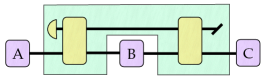
Figure 1: A three-time quantum process involving state preparation and two gates acting on both systems.

Let us label $A,B,C$ the times at which the operations take place. The operations are represented by general completely positive (CP), trace-non-increasing maps from an input to an output Hilbert space so that, for example at time $A$, the joint input-output space is $\mathcal{H}^{A}=\mathcal{H}^{A_{I}}\otimes\mathcal{H}^{A_{O}}$. The map can be expressed in Choi form [43, 44] (see Methods) as an operator $M^{A}_{a\mid x}\in\mathcal{L}(\mathcal{H}^{A})$, $M^{A}_{a\mid x}\geq 0$, where $a$ denotes the measurement outcome, $x$ denotes the setting (i.e., the choice of operation), and $\mathcal{L}(\mathcal{H})$ the space of linear operators over $\mathcal{H}$ [45]. For each setting choice $x$, a complete set of outcomes defines an instrument [46], expressed as a set $\{M^{A}_{a\mid x}\}_{a}$ such that $\sum_{a}\operatorname{Tr}_{A_{O}}M^{A}_{a\mid x}=\mathds{1}^{A_{I}}$. The process matrix is an operator on the joint space of all inputs and outputs, $W^{ABC}\in\mathcal{L}(\mathcal{H}^{A}\otimes\mathcal{H}^{B}\otimes\mathcal{H}^{C})$, $W^{ABC}\geq 0$, which allows one to calculate arbitrary joint probabilities for a sequence of outcomes $a,b,c$, given settings $x,y,z$, through the generalised Born rule [47]

$$p(a,b,c\mid x,y,z)=\operatorname{Tr}[W^{ABC}(M_{a\mid x}^{A}\otimes M_{b\mid y}^{B}\otimes M_{c\mid z}^{C})].$$ (1)

Formally, we can regard $W^{ABC}$ as a “density operator over time”, where each time instant corresponds to a pair of subsystems, an input and an output space. As output spaces encode the causal influence from an operation to future ones, the final output space can always be discarded (hence, the final time $C$ has only an input space). Furthermore in our scenario the first operation is a strong state preparation, which decorrelates the system from the environment allowing us to discard the first input space $A_{I}$. Thus for our experiment the process matrix is $W^{ABC}\equiv W^{A_{O}B_{I}B_{O}C_{I}}$ corresponding to a four-qubit state.

By selecting informationally complete instruments at each time, and exploiting the process-state isomorphism, one can reconstruct the process matrix using similar techniques as for ordinary state tomography, namely one can invert Eq. (1) and write $W$ as a function of the probabilities. A convenient choice for the instruments is projective measurements $\{\Pi_{a\mid x}\}_{a}$ immediately followed by the preparation of a state $\rho_{x}$, which correspond to operations of the form $M_{a\mid x}^{A}=\Pi_{a\mid x}^{A_{I}}\otimes\rho_{x}^{A^{T}_{O}}$, where $A^{T}_{O}$ denotes transposition on system $A_{O}$ and reflects our choice of convention, consistent with Eq. (1). This choice makes the protocol equivalent to tomography of a two-qubit channel that maps systems $A_{O}B_{O}$ to $B_{I}C_{I}$, with $W^{ABC}$ as its Choi matrix. As each measurement projects the system onto the measured state, at face value re-preparing an independent state requires a conditional qubit rotation. The fast feed-forward needed for this procedure was the main obstacle preventing full tomography in previous work [27, 28, 29, 30]. As detailed in the next section, we overcome this requirement through an appropriate post-processing scheme.

III Multi-time tomography protocol of a superconducting qubit

The experiment was conducted separately on two sets of superconducting hardware; an in-house processor at the University of Queensland, which will be referred to as uq, and a cloud processor from IBM Quantum with the moniker ibm_perth.

The experiment conducted on the uq processor used two capacitively-coupled flux-tunable transmons on a multi-qubit chip, mounted in a dilution refrigerator with a base temperature of around 15 mK. Each qubit is coupled to a dedicated resonator for readout. Flux lines are used in conjunction with a magnetic coil fixed to the chip to control transition frequencies, providing a degree of freedom by which qubit-qubit interaction strengths can be controlled.

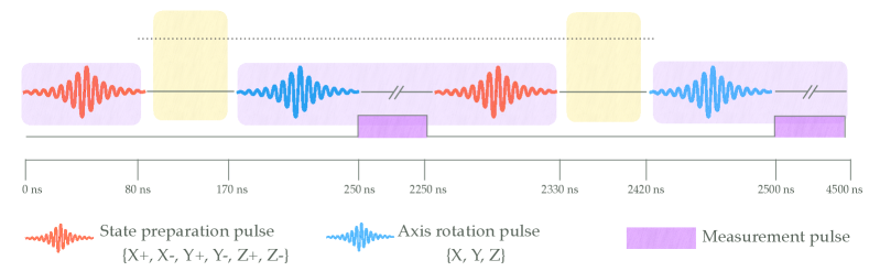
Figure 2: A visualisation of the pulse protocol used to generate tomography data. The solid line on which pulses are applied represents the system qubit. The dotted line represents the environment, with the two yellow boxes indicating the system-environment interaction that multi-time process tomography aims to characterise.

The experiments on the ibm_perth processor also utilised a two-transmon subset of a larger multi-qubit chip, but the system is comprised of fixed-frequency transmons. This removes flux control and thereby fixes the effective qubit interaction strength. In both experiments, the system of interest is a single qubit, while the other qubits are part of the environment (which also comprises any other degrees of freedom interacting with the system, as well as classical sources of noise).

To implement the three-time process tomography, we set the Pauli operators as our observables $\mathcal{M}=\{X,Y,Z\}$ and their eigenstates as the input states $\mathcal{B}=\{X_{+},X_{-},Y_{+},Y_{-},Z_{+},Z_{-}\}$. These form a tomographically (over) complete basis. We also define a set of operations within a basis gate set $\mathcal{G}=\{I,R_{X}(\pi/2),R_{X}(-\pi/2),R_{Y}(\pi/2),R_{Y}(-\pi/2),R_{X}(\pi)\}$. These operations are, by necessity, sufficient to prepare and measure all combinations of basis states and observables. Multi-time process tomography consists of temporally stacking two traditional process tomography protocols, forming a (prepare $\rightarrow$ process $\rightarrow$ measure $\rightarrow$ prepare $\rightarrow$ process $\rightarrow$ measure) protocol, where preparations are on spaces $A_{O},B_{O}$, while measurements are on $B_{I},C_{I}$. In these experiments, no operation is performed between each preparation and the subsequent measurement, so the idealised process is composed of two identity channels from $A_{O}$ to $B_{I}$ and from $B_{O}$ to $C_{I}$. Tomography aims to characterise departures from this idealisation, representing noise in the process due to system-environment interaction. The preparation states are drawn from $\mathcal{B}$ and measurement observables from $\mathcal{M}$, resulting in $\lvert\mathcal{B}\rvert^{2}\lvert\mathcal{M}\rvert^{2}=324$ unique protocols. The general form of this protocol is illustrated in Fig. 2, where we perform it on the system qubit (solid bottom line) and represent the environment with the top dotted line. Together with Fig. 1, we can see the multi-time quantum process and the times where we make the operations to gather the data.

To begin, all qubits were initialised in the ground state through a standard long wait-time routine. The system qubit is then prepared into some basis state $b_{0}\in\mathcal{B}$ using the appropriate rotation $p_{0}\in\mathcal{G}$. This occurs at $A$. The system and environment are then left to freely evolve for time $t_{1}$.

At $B$ we apply a projective measurement of the observable $m_{0}\in\mathcal{M}$ on the system qubit, consisting of some rotation gate $r_{0}\in\mathcal{G}$ to facilitate measurement of the correct axis, followed by a readout signal. The reflected readout signal is then classified as 0 or 1 and the result is stored in memory. After the mid-circuit measurement, another rotation $p_{1}\in\mathcal{G}$ is applied to prepare a new qubit state. Conditional on the eigenstate collapse in the mid-circuit measurement, this operation prepares the system qubit into one of the basis states $b_{1},\tilde{b}_{1}\in\mathcal{B}$. For example, if a protocol measures $m_{0}=X$ and applies rotation $p_{1}=I$, the prepared state is either $b_{1}=X_{+}$ or $\tilde{b}_{1}=X_{-}$. The actual prepared state is then identified by checking the result of the mid-circuit measurement. In this way, we are able to obtain a complete set of preparations over all experimental runs without the need for each prepared state to be chosen deterministically. This simple but critical post-processing technique is designed to avoid the need for dynamic, fast feed-forward control, which would otherwise be required for conditional operations. Following these operations, the system and environment are left to freely evolve for time $t_{2}$.

Finally, at $C$ we measure our second observable $m_{1}\in\mathcal{M}$. In all, the protocol is repeated 8192 times for each of 324 prepare-measure-prepare-measure permutations, resulting in approximately $5.3\times 10^{6}$ individual shots per process characterisation experiment (one on uq and nine at ibm_perth). This data is shaped into the number of realised counts we obtain for each of the 324 permutations. An example of these permutations is $(X_{+},X_{-},Y_{+},Z_{-})$ denoting that at $A$ we prepare the state $X_{+}$, at $B$ we projectively measure $X_{-}$ and then re-prepare $Y_{+}$, and at $C$ we projectively measure $Z_{-}$.

After obtaining the data, we are ready to calculate the experimental process matrix. A process matrix can written in the Pauli basis, $W=\sum_{i,j,k,l}\alpha_{i,j,k,l}\sigma_{i}\otimes\sigma_{j}\otimes\sigma_{k}\otimes\sigma_{l}$, where (i,j,k,l) = [0,3] denotes the Pauli basis ${\mathds{1},\sigma_{x},\sigma_{y},\sigma_{z}}$. From Eq. 1, we see that if we apply Pauli operations at $A,B,C$, their expectation values will be the coefficients $\langle\sigma_{i},\sigma_{j},\sigma_{k},\sigma_{l}\rangle=\alpha_{i,j,k,l}$. Hence, we can reconstruct the experimental process matrix, by calculating the expectation values of the sigma terms from the experimental data

$$W_{exp}=\frac{1}{16}\sum_{i,j,k,l}\langle\sigma_{i},\sigma_{j},\sigma_{k},\sigma_{l}\rangle\sigma_{i}\otimes\sigma_{j}\otimes\sigma_{k}\otimes\sigma_{l}.$$ (2)

$W_{exp}$ is the process matrix we construct from the experimental data, but it typically does not represent a physical one (it might be non-positive, or fail the process matrix constraints). To obtain a physical process, $W_{phys}$, we use SemiDefinite Programming (SDP), where we find a positive matrix that minimises its distance (we used Frobenius distance) with the $W_{exp}$. The SDP is the following:

variable $$W_{phys}$$ Hermitian Semidefinite

minimize $$\ \ \texttt{Frobenius Norm}(W_{exp}-W_{phys})$$ (3)

subject to $$\ \ L_{V}(W_{phys})==W_{phys}$$

$$\ \ \text{Tr}(W_{phys})==4,$$

where $L_{V}$ is an operator that projects a matrix to the space of valid process matrices [32] and the normalisation constraint helps the SDP to bound the solution. Using the $W_{phys}$ we report in the Results section our findings on tomography and non-Markovianity.

Our tomography protocol differs from related works in that we implement full multi-time process tomography by reconstructing the full process matrix. Concretely, Xiang et al. implement projective mid-circuit measurements but limit their analysis to an under-complete set of POVMs to construct a ‘restricted’ process matrix [28]. Similarly, White et al. restrict their tomography to only sequences of unitary operations and final measurement, with reference to the difficulty of mid-circuit measurement in superconducting processors [30]. Related work by the same authors extends their analysis to non-unital maps by introducing an ancillary qubit and entangling operations, obtaining a separate class of restricted information known as classical shadows [29].

IV Results: Tomography and non-Markovian noise

Figure 3 provides insight into the qualitative differences between two experimental (physical) process matrices, $W_{phys}$, using data from the in-house uq processor and from the ibm_perth processor. The process matrix from ibm_perth is visually almost indistinguishable from a noiseless process with identity channels between the times $A$, $B$ and $C$, while the uq process maintains the qualitative structure of the identity channels with evident noise. This is a reflection of the operational fidelity of the processors, in conjunction with the significantly higher interaction strength between the system and the rest of the qubits on the uq processor (which was controlled by setting the appropriate qubit-qubit detuning).

Overall, we took tomographic data for one process on the uq processor and nine on ibm_perth with varying $t_{1}$ and $t_{2}$. Variations in free evolution times were explored after simulating each system with a simple one-qubit environment model and finding that both general and quantum non-Markovianity depend highly on these times, with a particular structure (see Methods). No such structure was observed in the experiments we conducted. This indicates that even though in both platforms the system qubit couples directly only to one other qubit, such interaction does not account for all environmental effects.

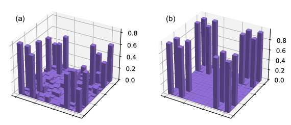
Figure 3: A visualisation of the absolute valued entries of the full multi-time process matrix, constructed with tomographic data from (a) the uq processor and (b) the ibm_perth processor.

Given the physical process matrices for each of the ten processes characterised (broadly denoted as $W_{phys}$), we aim to detect and quantify non-Markovianity. To this end, we calculate a measure of distance of each $W_{phys}$ with its closest Markovian process matrix $W_{M}$. We construct $W_{M}$ by discarding temporal correlations, combining the two channels  [30, 48]

$$W_{M}=T_{1}^{A_{O}B_{I}}\otimes T_{2}^{B_{O}C_{I}},$$ (4)

where $T_{1}^{A_{O}B_{I}}=Tr_{B_{O}C_{I}}W_{phys}$ and $T_{2}^{B_{O}C_{I}}=Tr_{A_{O}B_{I}}W_{phys}$. As a measure of distance, we consider the Jensen-Shannon divergence (JSD) for two matrices $W_{1}$ and $W_{2}$:

$$JSD\left(W_{1},W_{2}\right)=H\left(\frac{W_{1}+W_{2}}{2}\right)-\frac{1}{2}\left(H\left(W_{1}\right)+H\left(W_{2}\right)\right),$$ (5)

where $H(W)=-\operatorname{Tr}{W\log{W}}$ is the von Neumann entropy. The square root of the JSD operates as a distance measure between states or channels, and has utility in particular for quantifying non-Markovian dynamics [49]. The results for $\sqrt{JSD}$ across the ten processes are reported in Table 1. These indicates that non-Markovian effects were significant in both platforms for all choices of parameters, but were more pernicious on the uq processor. This is consistent with the appreciably stronger idle qubit-qubit interaction on this chip, as seen in Table 2.

	Evolution times	General non-Mark. noise	Quantum non-Mark. noise
	($t_{1},t_{2}$) ns	${\sqrt{JSD}}$ ${\times 10^{-1}}$	${\mathcal{N}}$ ${\times 10^{-2}}$
uq	(97, 97)	$5.04\pm 0.07$	$8.66\pm 0.86$
ibm_perth	(21, 21)	$1.77\pm 0.17$	$1.61\pm 0.58$
	(21, 24)	$1.64\pm 0.17$	$1.66\pm 0.61$
	(21, 28)	$1.81\pm 0.15$	$2.22\pm 0.69$
	(24, 21)	$1.60\pm 0.16$	$1.94\pm 0.64$
	(24, 24)	$1.85\pm 0.18$	$1.71\pm 0.65$
	(24, 28)	$2.06\pm 0.14$	$2.44\pm 0.68$
	(28, 21)	$1.96\pm 0.15$	$2.00\pm 0.71$
	(28, 24)	$1.85\pm 0.14$	$2.04\pm 0.67$
	(28, 28)	$1.76\pm 0.17$	$1.83\pm 0.62$

Table 1: The square root Jensen-Shannon divergence ($\sqrt{JSD}$) and negativity ($\mathcal{N}$) of the multi-time process matrices reconstructed for each processor. Each experiment characterises two periods of free evolution, which are denoted by labels $t_{1}$ and $t_{2}$, shown in nanoseconds. The ibm_perth data consisted of nine different experimental runs with slightly varying free evolution times, for the purposes of comparison to a theoretical model.

A natural subsequent inquiry is whether non-Markovianity originates from a quantum source; the value of distinguishing between classical or quantum environments lies in the manifestly different dynamics they induce [50, 51, 52, 53]. The quantum nature of non-Markovianity in the process is captured by quantum correlations across the evolution from $A$ to $B$ and from $B$ to $C$. This maps to entanglement across the bipartition $A_{O}B_{I}|B_{O}C_{I}$ in the four-qubit state representation of the process, $\rho^{A_{O}B_{I}|B_{O}C_{I}}:=\frac{W^{ABC}}{\operatorname{Tr}W^{ABC}}$ . To measure entanglement, we take the computationally inexpensive metric of negativity,

$$\mathcal{N}(\rho)=\left\lvert\sum_{\lambda_{i}<0}\lambda_{i}\right\rvert=\sum_{i}\frac{\lvert\lambda_{i}\rvert-\lambda_{i}}{2},$$ (6)

where $\rho=\rho^{(A_{O}B_{I})^{T}|B_{O}C_{I}}$, where $T$ denotes partial transposition (it can be on either of the two subsystems, $A_{O}B_{I}$ or $B_{O}C_{I}$), and $\lambda_{i}$ are the eigenvalues of $\rho$ [54].

Quantum multi-time correlations are observable on each processor, but they are markedly enhanced on the uq processor. This is again consistent with the increased interaction strength observed between the system qubit and its primary interacting ‘memory’ qubit on the uq processor as documented in Table 2. The negativities reported over the nine ibm_perth runs all lay within each others’ credible intervals, indicating that the quantum non-Markovianity present in each process was effectively invariant across the ($t_{1}$, $t_{2}$) landscape explored. In all measurements, the reported uncertainty denotes 95% credible intervals determined by bootstrapping techniques as described in Methods, accounting for sampling noise.

Using the natural log in Eq. 5, the $\sqrt{JSD}$ metric is bounded between 0 and $\log{2}$ [55], lending scale to the magnitude of our findings which lie on the order of $10^{-1}$. This is a strong signal that the multi-time processes characterised on each device are easily distinguishable from the most likely temporally uncorrelated candidates. Negativity serves as an entanglement monotone and is therefore bounded from below by zero (completely separable) [54]. The monotonic nature of negativity means that, in the case of states, it is upper bounded by the negativity of the maximally entangled state, which for four qubits is $\frac{3}{2}$, roughly two orders of magnitude larger than in our measurements. This state does not correspond to a valid process matrix (because the space of states is larger than that of process matrices) but it gives a sense of measure of our results on negativity, which are two orders of magnitude lower than the state maximum.

In summary, we observe and quantify non-Markovian dynamics and quantum correlations with high confidence on both uq and ibm_perth processors, reinforcing the importance of correlated noise in the design of mitigation techniques. Our results, interpreted alongside the bounds provided, demonstrate the practicality of our methods for characterising this noise.

V Conclusion

We report the first experimental full characterisation of a multi-time quantum process on a superconducting qubit. We implement ten three-time processes using an in-house superconducting processor and a cloud processor from IBM Quantum. We characterise the processes using the process matrix formalism and provide a measure of their non-Markovian noise; both general and stemming from quantum correlations across time. We find that non-Markovian noise is present in all cases, with a significant proportion originating from genuine quantum correlations. A comparison with a simple system-environment model indicates that the influence of nearest-neighbour qubits is not sufficient to account for all the observed quantum non-Markovianity. Our results demonstrate the capacity of our methods to fully describe multi-time processes and confidently measure and characterise non-Markovian noise, laying the foundation for novel error-mitigation techniques set to impact current and future quantum devices.

Methods

Experimental devices

The primary device used was a superconducting quantum processor consisting of five flux-tunable transmons, fabricated by Quantware [56]. System characteristics of the transmon we performed multi-time tomography on (‘System’) and the dominant interacting transmon (‘Memory’) are provided in Table 2. These characteristics include T1 and T2, the relaxation and dephasing lifetimes. The ‘System’ qubit only has one nearest-neighbour coupling to the ‘Memory’ qubit, which in turn is coupled to two other qubits. Charge lines and flux lines to each qubit permit XY control and frequency tunability respectively. A common feedline couples to individual dedicated resonators for each transmon qubit.

The custom-built open-source library sqdtoolz [57] is used to orchestrate the array of high-precision instruments required to execute control protocols on our quantum processor. This includes the synchronised generation and timing of microwave-frequency pulsed signals for control and measurement, a continuous microwave-frequency pump signal for parametric amplifier operation and a stable DC signal for frequency tuning purposes.

Characteristic	System qubit	Memory qubit
Symmetry point frequency	5.97 GHz	5.03 GHz
Operational frequency	5.11 GHz	5.03 GHz
Coupling to system	N/A	11 MHz
T1 (relaxation time)	14 $\mu$s	10 $\mu$s
T2 (dephasing time)	1.8 $\mu$s	6 $\mu$s

Table 2: The characteristics of the major interacting transmon qubits in the experimental processor. The system qubit is operating at a transition frequency far from its symmetry point, which increases its sensitivity to flux noise and in turn reduces T2.

Experiments are also performed on the cloud 7-qubit quantum processor ibm_perth, as provided by IBM Quantum [37]. This system offers increased coherence times and gate fidelities at the expense of frequency control. Transmon characteristics can be found in Table 3.

Characteristic	System qubit	Memory qubit
Qubit frequency	5.16 GHz	4.98 GHz
Coupling to system	N/A	3 MHz
T1 (relaxation time)	207 $\mu$s	102 $\mu$s
T2 (dephasing time)	295 $\mu$s	113 $\mu$s

Table 3: The characteristics of the major interacting transmon qubits in the IBM cloud processor. For this system, we have no control over frequency and therefore no control over interaction strength.

Error estimation

The credible intervals reported in Table 1 were calculated using the non-parametric resampling technique of bootstrapping. Bootstrapping a standard deviation for some metric $\hat{\theta}(\hat{X})$ relies on the assumption that the relative frequency of the measured $\hat{X}$ is representative of the underlying distribution which $\hat{X}$ is drawn from. In our case, $\hat{X}$ is a measured set of shot probabilities, which may look something like $\{$00: 0.7773, 10: 0.1738, 01: 0.0421, 11: 0.0068$\}$, where, 00 for example corresponds to the probability of getting the plus state in both measurements at $B$ and $C$. We resample 8000 shots from a multinomial distribution with these underlying relative frequencies, over 1000 trials, creating a set of bootstrapped results $\hat{X}_{i}$. The simulated distribution of the metric of interest is then evaluated as $\hat{\theta}(\hat{X}_{i})$ and twice the standard deviation of this distribution is used to calculate the 95% credible interval of the reported metric $\hat{\theta}(\hat{X})$. This technique is designed to account for shot noise in the finite-sample estimates of observables, and does not account for systematic error at the hardware level (gate miscalibration, readout misclassification). Finally, we rely on bias correction in the bootstrapping process; the sample mean of the metric $\hat{\theta}(\hat{X}_{i})$ was in general not equal to the measured $\hat{\theta}(\hat{X})$ (sometimes outside of the credible interval).

Simulated process

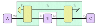
Figure 4: A three-time quantum process involving state preparation and two gates acting on both systems.

In both platforms used, the qubit we probe belongs to a larger multi-qubit array. The particular qubits we choose each have one nearest-neighbour qubit, with which they are directly coupled, as well as additional distant qubits (two or more degrees of separation), with which interactions will be weaker. We therefore take the simplest model of our environment to be that of the single coupled qubit, as shown in Fig. 4. This interaction can be described by the Hamiltonian [58]

$$H=\frac{\omega_{1}}{2}(\mathds{1}\otimes\sigma_{z})+\frac{\omega_{2}}{2}(\sigma_{z}\otimes\mathds{1})+g_{12}(\sigma_{+}\otimes\sigma_{-}+\sigma_{-}\otimes\sigma_{+}),$$ (7)

where $\omega_{1,2}$ are the resonance frequencies of the system and memory qubit, respectively, and $\sigma_{+,-}$ are the creation and annihilation operators, respectively. Then the free evolution of system-memory is expressed as $U=\exp{-iHt}$, where $t$ is the time of the evolution.

To write the process matrix for our system, we start with writing the terms: the initial state of the environment $\rho^{E_{1}}$, the channel $T_{1}^{A_{O}E_{1}^{T}B_{I}E2}$ and the second channel $T_{2}^{B_{O}E_{2}^{T}C_{I}E_{3}}$ (see Fig 4), where the superscript $T$ on a system denotes partial transposition for that system. To obtain the process matrix, we combine the terms and trace out all the environment systems

$$W=\text{Tr}_{E_{1},E_{2},E_{3}}(\rho^{E_{1}}\otimes T_{1}^{A_{O}E_{1}^{T}B_{I}E2}\otimes T_{2}^{B_{O}E_{2}^{T}C_{I}E_{3}}),$$ (8)

where $\rho^{E_{1}}=|{0}\rangle$ because all qubits on the chip are initialised to the ground state, $T_{1}^{A_{O}E_{1}B_{I}E2}=[[U]]^{A_{O}E_{1}B_{I}E2}$ and $T_{2}^{B_{O}E_{2}^{T}C_{I}E_{3}}=[[U]]^{B_{O}E_{2}C_{I}E_{3}}$, and $[[U]]$ is the Choi form of $U$, without the partial transposition.

Choi matrix definition: The Choi matrix $M^{A_{I}A_{O}}\in{\cal L}({\cal H}^{A_{I}}\otimes{\cal H}^{A_{O}})$, isomorphic to a CP map ${\cal M}^{A}:{\cal L}({\cal H}^{A_{I}})\rightarrow{\cal L}({\cal H}^{A_{O}})$ is defined as $M^{A_{I}A_{O}}:=[{\cal I}\otimes{\cal M}({{|{\mathds{1}}\rangle\!\rangle}\!{\langle\!\langle{\mathds{1}}|}}{\mathds{1}})]^{T}$, where $\cal I$ is the identity map, ${|{\mathds{1}}\rangle\!\rangle}=\sum_{j=1}^{d_{A_{I}}}|{jj}\rangle\in{\cal H}^{A_{I}}\otimes{\cal H}^{A_{I}}$, $\{|{j}\rangle\}^{d_{A_{I}}}_{j=1}$ is an orthonormal basis on ${\cal H}^{A_{I}}$ and ${T}$ denotes matrix transposition in that basis and some basis of ${\cal H}^{A_{O}}$.

We see that the free evolution, U, depends on the parameters of the Hamiltonian, $\omega_{1}$, $\omega_{2}$, $g_{1,2}$, and the time $t$. Hence, our process matrix will also depend on these parameters, $W(\omega_{1},\omega_{2},g_{1,2},t_{1},t_{2})$. To simulate the process on uq, experimental parameters were measured to be as given in Table 2, and we scan $t_{1}$ and $t_{2}$ from 85 to 115 ns, capturing the 97 ns process conducted in the experiment. For the process on ibm_perth, the parameters were fixed at the values available in Table 3, and we scan $t_{1}$ and $t_{2}$ between 17 and 33 ns, capturing the permutations of $t_{1}=[21.33,24.89,28.44]$ ns and $t_{2}=[21.33,24.89,28.44]$ ns conducted in experiment. The ibm_perth process simulation yielded the results in Fig. 5.

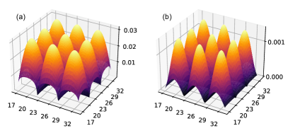
Figure 5: Simulated (a) $\sqrt{JSD}$ and (b) $\mathcal{N}$ values for the ibm_perth processor over a range of free evolution times $t_{1}$ and $t_{2}$.

According to these results, the experimental runs where evolution times are $t_{1}=t_{2}=24.89$ ns should maximise both metrics of non-Markovianity on ibm_perth, while other settings ($t_{1}=21.33$ ns and $t_{2}=28.44$ ns) should be close to fully suppressing non-Markovian dynamics. In practice, both metrics were observed to be smeared across the free evolution times scanned. This is not a particularly surprising result when contrasting the simplicity of the coupled-qubit environment described in Eq. 7 to the complexity of current-day quantum hardware, including but not limited to the extra qubits on each chip.

		max$({\sqrt{JSD}})$	max$({\mathcal{N}})$
uq	measured	0.504	0.087
	simulated	0.270	0.091
ibm_perth	measured	0.206	0.024
	simulated	0.031	0.001

Table 4: The maximum values observed for the square root Jensen-Shannon divergence ($\sqrt{JSD}$) and negativity ($\mathcal{N}$) across the experimentally measured (across the experimental runs, see Table 1) and simulated (at the peak of a ($t_{1}$, $t_{2}$) oscillation, see Fig. 5) multi-time processes.

A point of some interest is the comparison of the maximum $\sqrt{JSD}$ and $\mathcal{N}$ predicted in simulation (across a reasonable ($t_{1}$, $t_{2}$) range) to the values observed in experiment. A summary of the these are provided in Table 4. The qualitative structure of the simulated values match the results presented in this work, and are reasonable quantitatively on the uq processor. Both metrics are heavily underestimated on the ibm_perth processor. This is not an unusual result; the Hamiltonian presented in Eq 7 is certainly missing several terms, both characterisable (e.g. other qubits on the chip) and unknown. Hence, although the naive model is a reasonable first-order approximation, our results show that we can probe more complex dynamics than we can simulate, making our methods a powerful tool to detect non-Markovian noise.

References

- [1] J. Morris, F. A. Pollock, and K. Modi, Quantifying non-markovian memory in a superconducting quantum computer.
- McEwen et al. [2021] M. McEwen et al., Removing leakage-induced correlated errors in superconducting quantum error correction, Nature Communications 12, 10.1038/s41467-021-21982-y (2021).
- Young et al. [2020] K. Young, S. Bartlett, R. J. Blume-Kohout, J. K. Gamble, D. Lobser, P. Maunz, E. Nielsen, T. J. Proctor, M. Revelle, and K. M. Rudinger, Diagnosing and Destroying Non-Markovian Noise, Tech. Rep. (United States, 2020).
- Piilo et al. [2008] J. Piilo, S. Maniscalco, K. Härkönen, and K.-A. Suominen, Non-markovian quantum jumps, Phys. Rev. Lett. 100, 180402 (2008).
- Breuer et al. [2009] H.-P. Breuer, E.-M. Laine, and J. Piilo, Measure for the degree of non-markovian behavior of quantum processes in open systems, Phys. Rev. Lett. 103, 210401 (2009).
- Rivas et al. [2010] A. Rivas, S. F. Huelga, and M. B. Plenio, Entanglement and non-markovianity of quantum evolutions, Phys. Rev. Lett. 105, 050403 (2010).
- Rivas et al. [2014] Á. Rivas, S. F. Huelga, and M. B. Plenio, Quantum non-markovianity: characterization, quantification and detection, Rep. Prog. Phys. 77, 094001 (2014).
- Breuer et al. [2016] H.-P. Breuer, E.-M. Laine, J. Piilo, and B. Vacchini, Colloquium: Non-markovian dynamics in open quantum systems, Rev. Mod. Phys. 88, 021002 (2016).
- Chruściński et al. [2011] D. Chruściński, A. Kossakowski, and A. Rivas, Measures of non-markovianity: Divisibility versus backflow of information, Phys. Rev. A 83, 052128 (2011).
- de Vega and Alonso [2017] I. de Vega and D. Alonso, Dynamics of non-markovian open quantum systems, Reviews of Modern Physics 89, 015001 (2017).
- Takeda et al. [2018] K. Takeda et al., Optimized electrical control of a si/sige spin qubit in the presence of an induced frequency shift, npj Quantum Information 4, 54 (2018).
- Freer et al. [2017] S. Freer et al., A single-atom quantum memory in silicon, Quantum Science and Technology 2, 015009 (2017).
- Savytskyy et al. [2023] R. Savytskyy et al., An electrically driven single-atom “flip-flop”qubit, Science Advances 9, eadd9408 (2023).
- Zwerver et al. [2022] A. M. J. Zwerver et al., Qubits made by advanced semiconductor manufacturing, Nature Electronics 5, 184 (2022).
- Philips et al. [2022] S. G. J. Philips et al., Universal control of a six-qubit quantum processor in silicon, Nature 609, 919 (2022).
- Oreshkov et al. [2012] O. Oreshkov, F. Costa, and Č. Brukner, Quantum correlations with no causal order, Nat. Commun. 3, 1092 (2012), arXiv:1105.4464 [quant-ph] .
- Oreshkov and Giarmatzi [2016] O. Oreshkov and C. Giarmatzi, Causal and causally separable processes, New J. Phys. 18, 093020 (2016).
- Giarmatzi and Costa [2021] C. Giarmatzi and F. Costa, Witnessing quantum memory in non-Markovian processes, Quantum 5, 440 (2021).
- Shrapnel et al. [2018a] S. Shrapnel, F. Costa, and G. Milburn, Quantum markovianity as a supervised learning task, International Journal of Quantum Information 16, 1840010 (2018a).
- Taranto et al. [2021] P. Taranto, F. A. Pollock, and K. Modi, Non-markovian memory strength bounds quantum process recoverability, npj Quantum Information 7, 149 (2021).
- Fux et al. [2021] G. E. Fux, E. P. Butler, P. R. Eastham, B. W. Lovett, and J. Keeling, Efficient exploration of hamiltonian parameter space for optimal control of non-markovian open quantum systems, Phys. Rev. Lett. 126, 200401 (2021).
- Figueroa-Romero et al. [2021] P. Figueroa-Romero, K. Modi, R. J. Harris, T. M. Stace, and M.-H. Hsieh, Randomized benchmarking for non-markovian noise, PRX Quantum 2, 040351 (2021).
- Milz et al. [2018] S. Milz, F. A. Pollock, and K. Modi, Reconstructing non-markovian quantum dynamics with limited control, Phys. Rev. A 98, 012108 (2018).
- Muñoz et al. [2022] R. N. Muñoz, L. Frazer, G. Yuan, P. Mulvaney, F. A. Pollock, and K. Modi, Memory in quantum dot blinking, Phys. Rev. E 106, 014127 (2022).
- Goswami et al. [2021] K. Goswami, C. Giarmatzi, C. Monterola, S. Shrapnel, J. Romero, and F. Costa, Experimental characterization of a non-markovian quantum process, Phys. Rev. A 104, 022432 (2021).
- Morris et al. [2022] J. Morris, F. A. Pollock, and K. Modi, Quantifying non-markovian memory in a superconducting quantum computer, Open Systems & Information Dynamics 29, 10.1142/S123016122250007X (2022).
- White et al. [2020] G. A. L. White, C. D. Hill, F. A. Pollock, L. C. L. Hollenberg, and K. Modi, Demonstration of non-markovian process characterisation and control on a quantum processor, Nature Communications 11, 10.1038/s41467-020-20113-3 (2020).
- Xiang et al. [2021] L. Xiang et al., Quantify the non-markovian process with intervening projections in a superconducting processor (2021).
- White et al. [2021] G. A. L. White, F. A. Pollock, L. C. L. Hollenberg, C. D. Hill, and K. Modi, From many-body to many-time physics (2021).
- White et al. [2022] G. White, F. Pollock, L. Hollenberg, K. Modi, and C. Hill, Non-markovian quantum process tomography, PRX Quantum 3, 10.1103/prxquantum.3.020344 (2022).
- Chiribella et al. [2013] G. Chiribella, G. M. D’Ariano, P. Perinotti, and B. Valiron, Quantum computations without definite causal structure, Phys. Rev. A 88, 022318 (2013), arXiv:0912.0195 [quant-ph] .
- Araújo et al. [2015] M. Araújo, C. Branciard, F. Costa, A. Feix, C. Giarmatzi, and Č. Brukner, Witnessing causal nonseparability, New J. Phys. 17, 102001 (2015).
- Procopio et al. [2015] L. M. Procopio, A. Moqanaki, M. Araújo, F. Costa, I. Alonso Calafell, E. G. Dowd, D. R. Hamel, L. A. Rozema, Č. Brukner, and P. Walther, Experimental superposition of orders of quantum gates, Nature Communications 6, 10.1038/ncomms8913 (2015).
- Rubino et al. [2017] G. Rubino, L. A. Rozema, A. Feix, M. Araújo, J. M. Zeuner, L. M. Procopio, Č. Brukner, and P. Walther, Experimental verification of an indefinite causal order, Science Advances 3, e1602589 (2017).
- Goswami et al. [2018] K. Goswami, C. Giarmatzi, M. Kewming, F. Costa, C. Branciard, J. Romero, and A. White, Indefinite causal order in a quantum switch, Physical Review Letters 121, 10.1103/physrevlett.121.090503 (2018).
- Antesberger et al. [2023] M. Antesberger, M. T. Quintino, P. Walther, and L. A. Rozema, Higher-order process matrix tomography of a passively-stable quantum switch (2023), arXiv:2305.19386 [quant-ph] .
- IBM Quantum [2023] IBM Quantum, (2023).
- Chiribella et al. [2009] G. Chiribella, G. M. D’Ariano, and P. Perinotti, Theoretical framework for quantum networks, Phys. Rev. A 80, 022339 (2009), arXiv:0904.4483 [quant-ph] .
- Costa and Shrapnel [2016] F. Costa and S. Shrapnel, Quantum causal modelling, New J. Phys. 18, 063032 (2016).
- Gutoski and Watrous [2006] G. Gutoski and J. Watrous, Toward a general theory of quantum games, in In Proceedings of 39th ACM STOC (2006) pp. 565–574, quant-ph/0611234 .
- Pollock et al. [2018] F. A. Pollock, C. Rodríguez-Rosario, T. Frauenheim, M. Paternostro, and K. Modi, Non-markovian quantum processes: Complete framework and efficient characterization, Physical Review A 97, 012127 (2018).
- Lindblad [1979] G. Lindblad, Non-markovian quantum stochastic processes and their entropy, Comm. Math. Phys. 65, 281 (1979).
- Jamiołkowski [1972] A. Jamiołkowski, Linear transformations which preserve trace and positive semidefiniteness of operators, Rep. Math. Phys 3, 275 (1972).
- Choi [1975] M.-D. Choi, Completely positive linear maps on complex matrices, Linear Algebra and its Applications 10, 285 (1975).
- Heinosaari and Ziman [2011] T. Heinosaari and M. Ziman, The Mathematical Language of Quantum Theory: From Uncertainty to Entanglement (Cambridge University Press, 2011).
- Davies and Lewis [1970] E. B. Davies and J. T. Lewis, An operational approach to quantum probability, Communications in Mathematical Physics 17, 239 (1970).
- Shrapnel et al. [2018b] S. Shrapnel, F. Costa, and G. Milburn, Updating the born rule, New Journal of Physics 20, 053010 (2018b).
- Giarmatzi and Costa [2018] C. Giarmatzi and F. Costa, A quantum causal discovery algorithm, npj Quantum Information 4, 17 (2018).
- Settimo et al. [2022] F. Settimo, H.-P. Breuer, and B. Vacchini, Entropic and trace-distance-based measures of non-markovianity, Physical Review A 106, 10.1103/physreva.106.042212 (2022).
- Jouzdani and Mucciolo [2014] P. Jouzdani and E. R. Mucciolo, Numerical evaluation of the fidelity error threshold for the surface code, Phys. Rev. A 90, 012315 (2014).
- Paz-Silva et al. [2017] G. A. Paz-Silva, L. M. Norris, and L. Viola, Multiqubit spectroscopy of gaussian quantum noise, Physical Review A 95, 10.1103/physreva.95.022121 (2017).
- Beaudoin et al. [2018] F. Beaudoin, L. M. Norris, and L. Viola, Ramsey interferometry in correlated quantum noise environments, Phys. Rev. A 98, 020102 (2018).
- Paz-Silva et al. [2019] G. A. Paz-Silva, L. M. Norris, F. Beaudoin, and L. Viola, Extending comb-based spectral estimation to multiaxis quantum noise, Physical Review A 100, 10.1103/physreva.100.042334 (2019).
- Vidal and Werner [2002] G. Vidal and R. F. Werner, Computable measure of entanglement, Physical Review A 65, 10.1103/physreva.65.032314 (2002).
- Lin [1991] J. Lin, Divergence measures based on the shannon entropy, IEEE Transactions on Information Theory 37, 145 (1991).
- Quantware [2023] Quantware, (2023).
- Pakkiam et al. [2023] P. Pakkiam, R. Beriwal, and J. Dearlove, Sqdtoolz (2023).
- Blais et al. [2007] A. Blais, J. Gambetta, A. Wallraff, D. I. Schuster, S. M. Girvin, M. H. Devoret, and R. J. Schoelkopf, Quantum-information processing with circuit quantum electrodynamics, Physical Review A 75, 10.1103/physreva.75.032329 (2007).