Quadratic Dirac fermions and the competition of ordered states
in twisted bilayer graphene

Abstract

Magic-angle twisted bilayer graphene (TBG) exhibits a captivating phase diagram as a function of doping, featuring superconductivity and a variety of insulating and magnetic states. The bands host Dirac fermions with a reduced Fermi velocity; experiments have shown that the Dirac dispersion reappears near integer fillings of the moiré unit cell — referred to as the Dirac revival phenomenon. The reduced velocity of these Dirac states leads us to propose a scenario in which the Dirac fermions possess an approximately quadratic dispersion. The quadratic momentum dependence and particle-hole degeneracy at the Dirac point results in a logarithmic enhancement of interaction effects, which does not appear for a linear dispersion. The resulting non-trivial renormalisation group (RG) flow naturally produces the qualitative phase diagram as a function of doping – with nematic and insulating states near integer fillings, which give way to superconducting states past a critical relative doping. The RG method further produces different results to strong-coupling Hartree-Fock treatments: producing T-IVC insulating states for repulsive interactions, explaining the results of very recent STM experiments, alongside nodal $A_{2}$ superconductivity near half-filling, whose properties explain puzzles in tunnelling studies of the superconducting state. The model explains a diverse range of additional experimental observations, unifying many aspects of the phase diagram of TBG.

I Introduction

Twisted bilayer graphene (TBG) has become a central focus of theoretical and experimental condensed matter physics Cao2018a ; Cao2018b ; Yankowitz2019 ; Lu2019 ; Cao2020 ; Polshyn2019 ; Xie2019 ; Jiang2019 ; Choi2019 ; Kerelsky2019 ; Tomarken2019 ; Saito2021 ; Das2022 ; Cao2021b ; Paul2022 ; Wong2020 ; Morissette2023 ; Oh2021 ; Kim2022b ; Park2021c ; Nuckolls2023 ; Kim2023 ; Pierce2021 ; Stepanov2021 ; Bhowmik2022 ; Bhowmik2022 ; Choi2021 ; Nuckolls2020 ; Park2021 ; Xu2020 ; Xie2021 ; Das2021b ; Serlin2019 ; Polski2022 ; Saito2021b ; Sharpe2019 ; OrbMagReview ; Sharpe2021b ; Lin2022 ; Grover2022 ; Uri2020 ; Tschirhart2021 ; Kim2021 ; Po2018 ; Po2019 ; Xu2018 ; Tarnopolsky2019 ; Bernevig2021a ; Bernevig2021b ; Bernevig2021c ; Bernevig2021f ; Song2019 ; Song2022 ; Isobe2018 ; You2019 ; Liu2018 ; Gonzalez2019 ; Classen2019 ; Lin2019 ; Chichinadze2020 ; Chichinadze2020b ; Guinea2018 ; Bultinck2020 ; Bernevig2021d ; Bernevig2021e ; Kwan2021b ; Liu2021c ; Liu2021b ; PhononsTIVC ; Wagner2022 ; Christos2022 ; BernevigTrilayer ; TBorNotTB ; Yu2023 ; Peltonen2018 ; Xu2018kek ; Lian2019 ; Wu2018 ; Zhang2019 ; Yuan2018 ; Kang2019 ; Ahn2019 ; Julku2020 ; Padhi2020 ; Fernandes2021 ; Kwan2021 ; Padhi2018 ; Thomson2021 ; Yu2021 ; Khalaf2022 ; Mathias2020 ; Lake2022 ; Zhang2019b ; Lee2019 ; Christos2023 ; Roy2019 ; Islam2023 ; Brillaux2022 ; Parthenios2023 . Since the original discovery of unconventional superconductivity and correlated insulating states Cao2018a ; Cao2018b , intense experimental scrutiny has uncovered a rich phase diagram as a function of temperature, electron density, and magnetic field – featuring orbital magnetism, nematic ordering, and Kekulé textures Cao2018a ; Cao2018b ; Yankowitz2019 ; Lu2019 ; Cao2020 ; Polshyn2019 ; Xie2019 ; Jiang2019 ; Choi2019 ; Kerelsky2019 ; Saito2021 ; Das2022 ; Cao2021b ; Paul2022 ; Wong2020 ; Morissette2023 ; Tomarken2019 ; Oh2021 ; Kim2022b ; Park2021c ; Nuckolls2023 ; Kim2023 ; Pierce2021 ; Stepanov2021 ; Bhowmik2022 ; Bhowmik2022 ; Choi2021 ; Nuckolls2020 ; Park2021 ; Xu2020 ; Xie2021 ; Das2021b ; Serlin2019 ; Polski2022 ; Saito2021b ; Sharpe2019 ; OrbMagReview ; Sharpe2021b ; Lin2022 ; Grover2022 ; Uri2020 ; Tschirhart2021 ; Kim2021 .

Stacking two sheets of graphene and twisting by a relative angle $\theta$, the composite system is no longer periodic with the lattice constant of monolayer graphene, but is periodic at a larger moiré scale $\sim a/(2\sin(\theta/2))$, folding the monolayer graphene dispersion into a mini Brillouin zone Santos2012 ; Bistritzer2011 ; Koshino2018 ; Po2018obstr ; Khalaf2019idk ; Yoo2019 ; Tritsaris2020 ; Carr2019b ; Carr2019 ; Kang2018 ; Zang2022 . The coupling between the two layers hybridises the monolayer Dirac points of graphene, forming mini bands, and when the twist angle is reduced to the so-called magic angle, the fourfold degenerate bands near charge neutrality flatten and the velocity of the Dirac points grows small, enhancing interaction effects and giving rise to a diverse collection of interesting material properties.

Compressibility measurements observe an interesting property of TBG referred to as the Dirac revival – when the density of electrons is increased to an integer number of electrons per unit cell, additional electrons ‘reset’ to the charge neutrality point, and are described by the Dirac dispersion but with a reduced degeneracy Zondinger2020 . For instance, at one electron per moiré unit cell $\nu=1$ (Fig. 2), one of the four-fold degenerate bands spontaneously becomes fully occupied, and as the density is increased the remaining three-fold degenerate bands refill starting from the charge neutrality point endnote1 . These revived Dirac fermions appear at much higher temperatures ($\approx 20$ K) than the insulating and superconducting states ($\approx 1$ K), and constitute the parent state of the correlated physics.

Figure 1: Theoretical model. Left: Two stacks of graphene with a relative twist of $\theta$, Right: Our model for the Dirac fermions near integer filling. The dispersion is linear beneath an infrared cutoff $\Lambda_{v}$, and quadratic between $\Lambda_{v}$ and an ultraviolet cutoff $\Lambda$. In the temperature window $\Lambda_{v}<T<\Lambda$, interactions are logarithmically enhanced. Middle: Our proposed phase diagram features interlaced superconductors (red) and correlated insulators (blue), including nematic/K-IVC order at $\nu=0$ and T-IVC order with proximate $E$/$A_{2}$ superconductivity near $\nu=2$.

While the magic angle tunes the Fermi velocity to be small, there is nonetheless a nonzero bandwidth; we suggest that the smallness of the linear term in the Dirac dispersion makes the dispersion approximately quadratic for an energy window near the Dirac points (Fig. 1c). Due to the Dirac revival, the quadratic Dirac dispersion near charge neutrality then characterises the physics of TBG near all integer fillings. A quadratic dispersion plus particle-hole degeneracy at the Fermi level in two dimensions results in a logarithmic enhancement of interaction effects, and a non-trivial renormalisation group (RG) flow. In this work we analyse the RG flow of these quadratic Dirac fermions and derive a number of interesting results:

1. Near integer fillings, the particle-hole degeneracy of the Dirac point causes insulating and nematic states, driven by particle-hole fluctuations, to compete strongly against superconductivity. Doping above the Dirac point lifts the particle-hole degeneracy, leaving superconductivity as the dominant order.

2. The result is a phase diagram with nematic or insulating states at integer fillings and superconductors in between (see Fig. 1b), consistent with the experimentally obtained phase diagram of TBG.

3. The quadratic Dirac theory predicts different ground states to pre-existing mean-field analyses; we list the resulting order parameters in Table 1. For instance, Hartree-Fock studies of the Coulomb repulsion favour K-IVC over T-IVC Guinea2018 ; Bultinck2020 ; Bernevig2021d ; Bernevig2021e ; Kwan2021b ; Liu2021c ; Liu2021b ; PhononsTIVC ; Wagner2022 ; Christos2022 , requiring phonon coupling for T-IVC to contend, whereas the RG flow can favour T-IVC for purely repulsive interactions. Very recent STM experiments have found evidence for T-IVC rather than K-IVC order near $\nu=2$ Nuckolls2023 ; Kim2023 ; our mechanism therefore provides a natural explanation of this puzzle.

4. Intervalley $A_{2}$ and $E$ superconductors appear as instabilities alongside T-IVC order near $\nu\gtrsim 2$; the properties of the $A_{2}$ state can explain the transition from U- to V- shaped tunnelling profiles seen in studies of the superconducting state Oh2021 ; Kim2022b ; Park2021c .

Incorporating a small finite Dirac velocity does not dramatically modify the RG behaviour of the Dirac theory, simply introducing an IR cutoff $\Lambda_{v}$ on the RG flow. The enhancement of the interactions occurs within a window of temperatures associated to the energy window in which the dispersion appears quadratic (c.f. Fig. 1c).

We contrast our theory with previous theoretical models. Firstly, interacting theories with linearly-dispersing Dirac fermions (e.g. Refs. Roy2019 ; Islam2023 ; Brillaux2022 ; Parthenios2023 ) do not naturally feature insulating and nematic states as weak coupling instabilities. As we explain in Sec III, the quadratic scaling of the dispersion is essential to the presence of insulating and nematic states near integer fillings. Secondly, the starting point of our analysis is to treat the bands as dispersive rather than approximately flat (c.f. Refs Kang2019 ; Bultinck2020 ; Bernevig2021d ; Christos2022 ; TBorNotTB ), motivated by the experimental observation of dispersive Dirac states Zondinger2020 , and a bandwidth $\approx 40$ meV, much larger than that predicted by bandstructure Tomarken2019 . Thirdly, we stress that van Hove singularities (vHS) and Fermi surface nesting Isobe2018 ; You2019 ; Liu2018 ; Gonzalez2019 ; Classen2019 ; Lin2019 ; Chichinadze2020 ; Chichinadze2020b do not feature in our model. Since the Dirac revival resets the dispersion to that of the Dirac point near integer fillings, in this regime the Fermi surface is neither nested nor located near a vHS. Experiments have found that superconductivity is seen near resets, and consistently suppressed at twist angles where revivals disappear and vHS are observed endnote2 .

By contrast, our model argues that the superconducting and insulating states arise from the RG flow from a quadratic dispersion, with superconductivity dominant when the insulating states are suppressed via doping. Superconductivity therefore does not originate from an insulating parent state, but appears as a competing phase. The competing order scenario is supported by the presence of superconductivity in the absence of insulating states at smaller twist angles or when TBG is strongly screened by external gates Liu2021 ; Stepanov2020 ; Saito2020b (though we comment that interpretation of these experiments is complicated by the presence of disorder), the appearance of the insulating state under the superconducting dome when superconductivity is suppressed by a magnetic field, along with the comparable magnitudes of the superconducting and insulating $T_{c}$. Given this last point, it is particularly notable that our framework allows a simultaneous treatment of the insulating and superconducting states on equal footing, unlike Hartree-Fock studies which are well-suited to describing the insulating states.

We lastly note that signatures of the Dirac revival phenomena are also seen in twisted trilayer graphene (tTLG) Park2021a ; Hao2021 ; Cao2021a ; Siriviboon2021 ; Zhang2021b , and so we anticipate that our analysis is likely relevant to a range of moiré systems.

II Model and symmetry constraints

II.1 Quantum numbers and Symmetries

The bands near charge neutrality are four-fold degenerate, originating from the spin and monolayer valley degeneracy. The conduction and valence bands exhibit Dirac points at the moiré $K$-points; we index these band touching points by sublattice $\sigma$, monolayer valley $\tau$, and moiré valley $\eta=\pm$, corresponding to the Bloch states near quasimomenta $\tau R_{\pm\theta/2}\bm{K}$ where $\bm{K}$ is the monolayer valley momentum. Counting the number of Dirac cones gives $N_{f}=8$ species of Dirac fermions (see Fig. 2 left).

We describe the valley and spin quantum numbers as “flavours”; after each Dirac revival, a flavour is projected out reducing the degeneracy by two, as shown in Fig. 2, i.e. $N_{f}=2(4-\lfloor\nu\rfloor)$ for $\nu>0$. In our analysis, we will not attempt to explain the origins of the revivals, but take the polarised Dirac theory as an input parent state. It is observed (e.g. Ref. Polski2022 ) that this parent state appears at different angles for electron $\nu>0$ and hole $\nu<0$ doping. Our argument that the correlated phases arise from the revived Dirac parent state therefore naturally explains the observed electron-hole asymmetry of the superconducting phase diagram. In what follows we will take $\nu>0$ with the understanding that our results apply to all integer $-4<\nu<4$ at which revivals occur.

Figure 2: Dirac revival. At each moiré valley $\eta=\pm$ there are four flavours corresponding to the spin $s=\pm$ and monolayer valley $\tau=\pm$ degeneracy, which for $|\nu|\gtrsim 0$ populate equally as the density increases (Left). When the bands are quarter filled at $|\nu|=1$, all the density is spontaneously transferred to one flavour, and any additional electrons are added near the band touching point of the remaining Dirac states (Right).

TBG possesses threefold rotational symmetry in the plane $C_{3z}$, twofold rotational symmetry about the $x$ axis $C_{2x}$, twofold rotational symmetry in the plane $C_{2z}$, i.e. the $D_{6}$ point group, along with time-reversal symmetry $\Theta$ (TRS). The system maintains SU(2) spin rotational symmetry due to absence of spin-orbit coupling. In addition, TBG has approximate symmetries, which we shall take to be exact in our model: independent spin rotations in the two monolayer valleys results in an enlarged SU(2)$\times$ SU(2) spin symmetry. This symmetry is broken in experiment by the small yet finite Hund’s coupling $J_{H}$. In the small twist angle limit, TBG also possesses a particle-hole symmetry ${\cal P}$ endnote3 ; combining particle-hole and TRS gives an anti-commuting chiral symmetry represented by ${\cal S}=\mathcal{P}\Theta=\sigma_{x}\tau_{x}\eta_{y}$, with action ${\cal S}{\cal H}_{0}(\bm{k}){\cal S}^{\dagger}=-{\cal H}_{0}(\bm{k})$ on the single-particle Hamiltonian $\mathcal{H}_{0}$.

II.2 Single-particle Hamiltonian

The above symmetries allow us to construct the most general single-particle Hamiltonian describing the Dirac states near the moiré $K$-points, which to quadratic order we find to be

$$\mathcal{H}_{0}=v\tau_{z}(k_{+}\alpha_{-}+k_{-}\alpha_{+})+i\beta\eta_{z}\left(k_{+}^{2}\alpha_{+}-k_{-}^{2}\alpha_{-}\right)$$ (1)

where $(\alpha_{x},\alpha_{y})=(\sigma_{x},\tau_{z}\sigma_{y})$, $\alpha_{\pm}=\alpha_{x}\pm i\alpha_{y}$, and $k_{\pm}=k_{x}\pm ik_{y}$. Strikingly, we find that restricting to quadratic order in the momentum expansion results in an emergent commuting chiral symmetry $[{\cal C},\mathcal{H}_{0}]=0$ with ${\cal C}=-i\sigma_{z}{\cal S}=\sigma_{y}\tau_{x}\eta_{y}$; terms which break this symmetry may only appear at cubic and higher order in momentum. The symmetry ${\cal C}$ has been studied in previous works, where a so-called ‘chiral limit’ Tarnopolsky2019 results in ${\cal C}$ as an exact symmetry endnote4 . Here we do not impose the chiral limit, yet we find that this symmetry appears as an emergent low-energy symmetry of the Dirac effective theory.

Our approach shall be to assume $\Lambda_{v}=v^{2}/\beta$ is small compared to the UV cutoff $\Lambda\gg\Lambda_{v}$, so that there is a range of energies in which the dispersion can be treated as quadratic, allowing us to neglect the linear term, Fig. 1c. In TBG, there are natural reasons to expect $\Lambda\gg\Lambda_{v}$ – in the limit where $\mathcal{P}$ is taken to be an exact symmetry, it has been shown Raquel that the velocity can be made to vanish by tuning only a single parameter. Motivated by these results, in the Supplementary Material we show that for a wide range of tunnelling couplings, the $\mathcal{P}$-symmetric Bistritzer-MacDonald model Bistritzer2011 possesses a twist angle at which the Dirac points exhibit a quadratic dispersion endnote5 . However, our results are not reliant on the exact values of $v$ and $\beta$ – we shall leave them as phenomenological constants, which may feasibly be investigated experimentally through compressibility measurements shahal .

II.3 Interactions

Projecting the Coulomb interaction onto the basis of states near the Dirac points $|\sigma,\tau,\eta\rangle$ gives

$$V=\tfrac{1}{2}\sum_{\mu\nu}V_{13;24}\psi^{\dagger}_{1,\bm{k}}\psi_{3,\bm{k}-\bm{q}}\psi^{\dagger}_{2,\bm{p}}\psi_{4,\bm{p}+\bm{q}}$$ (2)

where $1$,$2$,$3$,$4$ are shorthand for the indices $\{\sigma,\tau,\eta\}$. A powerful approach is to write the interactions in the adjoint representation:

$$V_{13;24}=V_{\mu\nu}\,(\Omega^{\mu})_{13}(\Omega^{\nu})_{24}$$ (3)

where $\Omega^{\mu}\in\{\sigma_{a}\tau_{b}\eta_{c}\}$, representing the Coulomb potential as a sum of tensor products in $\sigma\tau\eta$ space Li2020 ; Scammell2021 ; Li2020b . The potential is constrained by the requirement that only symmetry-invariant tensor products appear; in the Supplementary Material, we list the full set of symmetry-allowed products of bilinears. Under the assumption of a real Coulomb potential, only $\Omega^{\mu}$ which commute with $\mathcal{S}$ and $\cal C$ may appear. These constraints result in only three possible bilinears: $\Omega^{\mu}\in\{\sigma_{0}\tau_{0}\eta_{0},\sigma_{z}\tau_{0}\eta_{z},\sigma_{z}\tau_{0}\tilde{\eta}_{\pm}\}$, where $\tilde{\eta}_{\pm}=\eta_{x}\pm i\tau_{z}\eta_{y}$. Renormalisation of the interactions, which we discuss further in the next section, generates the additional vertices $\eta_{z}\alpha_{x}\Omega^{\mu},\eta_{z}\alpha_{y}\Omega^{\mu},\alpha_{z}\Omega^{\mu}$, which commute with $\cal C$ but not $\cal S$. This results in a set of nine coupling constants,

$$V=g_{o}(\sigma_{0}\tau_{0}\eta_{0}\otimes\sigma_{0}\tau_{0}\eta_{0})+g_{x\tau}(\alpha_{\pm}\tau_{z}\eta_{0}\otimes\alpha_{\mp}\tau_{z}\eta_{0})+g_{z}(\alpha_{z}\tau_{0}\eta_{0}\otimes\alpha_{z}\tau_{0}\eta_{0})$$

$$+\,v_{o\tau}(\sigma_{0}\tau_{z}\tilde{\eta}_{\pm}\otimes\sigma_{0}\tau_{z}\tilde{\eta}_{\mp})+v_{x}(\alpha_{\pm}\tau_{0}\tilde{\eta}_{\pm}\otimes\alpha_{\mp}\tau_{0}\tilde{\eta}_{\mp}+\alpha_{\pm}\tau_{0}\tilde{\eta}_{\mp}\otimes\alpha_{\mp}\tau_{0}\tilde{\eta}_{\pm})+v_{z}(\sigma_{z}\tau_{0}\tilde{\eta}_{\pm}\otimes\sigma_{z}\tau_{0}\tilde{\eta}_{\mp})$$

$$+u_{o\tau}(\sigma_{0}\tau_{z}\eta_{z}\otimes\sigma_{0}\tau_{z}\eta_{z})+u_{x}(\alpha_{\pm}\tau_{0}\eta_{z}\otimes\alpha_{\mp}\tau_{0}\eta_{z})+u_{z}(\sigma_{z}\tau_{0}\eta_{z}\otimes\sigma_{z}\tau_{0}\eta_{z}).$$ (4)

Based on the above arguments, our expectation is that $g_{o}$ and $v_{z}$ are likely the largest couplings near $\nu=0$, but after each Dirac revival the bare values of these couplings likely change. Our theory for TBG near integer filling comprises the single-particle Hamiltonian Eq. (1) along with the four-fermion interactions of Eq. (4), $\mathcal{H}=\mathcal{H}_{0}+V$. We argue this describes the normal state at each integer filling out of which the insulating and superconducting phases develop. Prior studies of Dirac theories Roy2019 ; Islam2023 ; Brillaux2022 ; Parthenios2023 have not explored the combination of quadratic band touching, $\eta$–dependent scattering, and filling factor-dependent degeneracy $N_{f}=2(4-\lfloor\nu\rfloor)$, which we now elucidate.

Figure 3: Flow equation. The approximately quadratic dispersion and particle-hole symmetry result in logarithmic divergences in each diagram. Removing particle-hole degeneracy by doping above the band-touching point weakens the latter three diagrams; we encode this effect approximately through a prefactor $d<1$. The RPA diagram $\propto N_{f}$ decreases after each Dirac revival.

III Renormalisation flow equations

The field theory we derived has a number of interesting properties. The combination of the band-touching Dirac states and momentum scaling of the energy $\propto k^{2}$ in two dimensions results in a logarithmic enhancement of interaction effects Yang2010 ; Sun2009 ; Wang2017 ; Uebelacker2011 ; PavelCuprates , analogous to how a linear dispersion in one dimension results in strongly interacting physics in the theory of Luttinger liquids Giamarchi2004 .

Corrections to the interaction constants are proportional to the so-called particle-particle and particle-hole susceptibilities,

$$\chi_{pp}(T)=\scaleobj{.95}{\sum_{n}}\scaleobj{.85}{\int}\mathcal{G}(i\omega_{n},\bm{k})\mathcal{G}(-i\omega_{n},-\bm{k})\,d^{2}$$

$$\chi_{ph}(T)=\scaleobj{.95}{\sum_{n}}\scaleobj{.85}{\int}\mathcal{G}(i\omega_{n},\bm{k})\mathcal{G}(i\omega_{n},\bm{k})\,d^{2}k$$ (5)

where $\mathcal{G}(i\omega_{n},\bm{k})$ is the Matsubara Green’s function,

$$\mathcal{G}(i\omega_{n},\bm{k})=\frac{1}{i\omega_{n}+\mu-i\beta\eta_{z}\left(k_{+}^{2}\alpha_{+}-k_{-}^{2}\alpha_{-}\right)},$$ (6)

and $\omega_{n}=(2n+1)\pi T$ are fermionic Matsubara frequencies. When the chemical potential is placed near the band-touching point, i.e. $\mu=0$, one finds that the scaling of the numerator $\sim d^{2}k$, and denominator $\sim\beta k^{2}$, results in $\chi_{pp}(T),\chi_{pp}(T)\rightarrow\log(\Lambda/T)/(4\pi\beta)$ as $T\rightarrow 0$ where $\Lambda$ is the UV cutoff, i.e. the corrections to the couplings diverge logarithmically. Doping away from the band-touching point via $\mu\neq 0$ weakens the divergence in $\chi_{ph}$ by removing the degeneracy of particle and hole excitations, while $\chi_{pp}$ remains logarithmically divergent.

By comparison, a linear dispersion would result in $\chi_{ph}\sim T$ as $T\rightarrow 0$, i.e. the associated corrections to the couplings would scale towards zero. In experiment, a small but finite velocity is observed; the effects of a finite velocity can be roughly incorporated as an IR cutoff on the RG flow $\Lambda_{v}\sim v^{2}/\beta$ – as the temperature is lowered from $\Lambda$ to $\Lambda_{v}$, the quadratic dispersion results in a logarithmic enhancement of interactions, and for temperatures lower than $\Lambda_{v}$ the enhancement ceases. Hence, there exists a window of temperatures in which the RG flow is controlled by the quadratic dispersion, c.f. Fig. 1.

To track the evolution of the effective couplings with temperature, we use the functional renormalisation group (fRG) method Platt2013 ; Metzner2012 ; Salmhofer2001 ; Polchinski1984 ; Wetterich1993 ; Kennes2019 ; Klebl2020 ; we derive the method from a path integral treatment in the Supplementary Material. The couplings become functions of the dimensionless RG time $t=\Lambda/T$, where the values at $t=1$ are the unrenormalised values, and $t\rightarrow\infty$ describes the low temperature behaviour of the theory. We find the RG equations can be written in the simple form reflected in Fig. 3; we obtain the analytic expression,

$$\tfrac{d}{dt}V_{\alpha\beta}\,\Omega_{\alpha}\otimes\Omega_{\beta}$$

$$=V_{\mu\nu}V_{\rho\lambda}(\dot{\Xi}_{\mu\nu;\rho\lambda}^{pp}+\dot{\Xi}_{\mu\nu;\rho\lambda}^{ph}+\dot{\Xi}_{\mu\nu;\rho\lambda}^{rpa}+\dot{\Xi}_{\mu\nu;\rho\lambda}^{vert})$$ (7)

where Einstein summation is implied for indices, and the matrix-valued RG kernels $\Xi_{\mu\nu;\rho\lambda}$ correspond to the Feynman diagrams in Fig. 3. The RG procedure is to take the bare interactions and evolve them according to (7) until they grow large, resulting in a diverging susceptibility for some order parameters and a concomitant phase transition to an ordered state (see Sec. IV). At weak coupling, this occurs as $t\rightarrow\infty$, and in this limit the fRG equations reduce to the well-known parquet equations Maiti2013 ; Classen2020 ; Schulz1987 ; Furukawa1998 ; Nandkishore2012 ; Wu2022 ; Li2022nest ; Scammell2023 . The RG flow predicts a divergence of the renormalised couplings as the flow proceeds into the deep IR, resulting in a re-emergence of strong coupling and a possible instability towards an ordered state.

The diagram $\Xi_{\mu\nu;\rho\lambda}^{pp}$ is the Cooper channel diagram $\propto\chi_{pp}$ familiar from Fermi liquid theory – the internal lines have opposite momenta, and the diagram is proportional to the “Cooper logarithm” which drives the superconducting instability. The other diagrams $\Xi_{\mu\nu;\rho\lambda}^{ph}$, $\Xi_{\mu\nu;\rho\lambda}^{rpa}$, $\Xi_{\mu\nu;\rho\lambda}^{vert}$ $\propto\chi_{ph}$ are the so-called “particle-hole” diagrams, which diverge as a result of particle-hole degeneracy and the quadratic dispersion. As one dopes away from the band touching point, the contribution of these diagrams is weakened via a cut-off on the logarithmic divergence. We encode this effect of doping by multiplying the particle-hole diagrams by a constant $d=d(\mu)\leq 1$ which equals $1$ at the band touching point and grows smaller with increased doping away from the band touching point i.e. increasing deviation from particle-hole degeneracy – a standard approximation in parquet RG endnote6 . Secondly, the RPA bubble diagram $\Xi_{\mu\nu;\rho\lambda}^{rpa}$ contains a fermionic trace which produces a factor $N_{f}$. After each Dirac revival, $N_{f}$ reduces by $2$, changing the renormalisation flow by weakening the RPA diagram, and altering the preferred ordered states near each integer filling.

Figure 4: Gap equations. Diagrams contributing to the superconducting and particle-hole order parameters. The particle-hole diagrams weaken upon doping away from integer filling, i.e. decreasing $d$, while the bubble diagram $\propto N_{f}=2(4-\lfloor\nu\rfloor)$.

IV Ordering instabilities of the Dirac theory

The ground state becomes unstable to an ordered phase when the associated order parameter develops a diverging susceptibility. The critical temperature for the ordered phase is given by $T_{c}=\Lambda/t_{c}$ where $t_{c}$ is the RG time at which the susceptibility diverges. The onset of an ordered state can be described by RG flow equations for the order parameter vertices, corresponding to the diagrams in Fig. 4, and take the form

$$\partial_{t}\mathcal{O}_{i} =\lambda_{i}(t)\,\mathcal{O}_{i}$$ (8)

$$\partial_{t}\Delta_{i} =\tilde{\lambda}_{i}(t)\,\Delta_{i}$$ (9)

where $\lambda_{i}(t)$ and $\tilde{\lambda}_{i}(t)$ are henceforth referred to as ‘order parameter eigenvalues’, and are expressions involving the renormalised couplings, as well as $\chi_{pp}$, and $\chi_{ph}$ (see the Supplementary Material). The susceptibilities for superconducting orders $\Delta_{i}\in\langle\psi\sigma_{\mu}\tau_{\nu}\eta_{\rho}\psi\rangle$ are driven to diverge by the particle-particle diagram $\propto\chi_{pp}$ in Fig. 4a, while susceptibilities for particle-hole orders $\mathcal{O}_{i}\in\langle\psi^{\dagger}\sigma_{\mu}\tau_{\nu}\eta_{\rho}\psi\rangle$ are driven to diverge by the particle-hole diagrams $\propto\chi_{ph}$ in Fig. 4b; the logarithmic divergences in these diagrams mean the $\Delta_{i}$ and $\mathcal{O}_{i}$ compete as weak coupling instabilities. The $\chi_{ph}$ in Fig. 4b are proportional to $d$ and get weaker away from integer filling; decreasing $d$ suppresses the tendency towards $\mathcal{O}_{i}$.

Considering now the role of Dirac revivals: First, the particle-hole diagram $\propto N_{f}$ changes after each Dirac revival, which has a non-trivial influence on the order parameters. Second, doping away from the band touchings at integer fillings decreases $\chi_{ph}$ via the factor $d$, suppresses the tendency towards $\mathcal{O}_{i}$; in other words, near the band-touching point, fluctuations of the degenerate particle and hole states promote insulating states $\mathcal{O}_{i}$, while doping away from the band-touching point weakens these fluctuations allowing superconductivity $\Delta_{i}$ to dominate. Lastly, after each Dirac revival, the order parameters and couplings are projected onto flavour polarised bands. Denoting the projection operator onto the remaining flavours as $\mathcal{P}_{f}$, the order parameters transform as $\mathcal{O}\rightarrow\mathcal{P}_{f}\mathcal{O}\mathcal{P}_{f}^{\dagger}$, $\Delta\rightarrow\mathcal{P}_{f}\Delta\mathcal{P}_{f}^{T}$. Since the operators $\mathcal{P}_{f}$ commute with the Hamiltonian, we can solve the RG equations in the unpolarised basis, then project the resulting order parameters onto the flavour polarised bands at a given filling.

To determine the leading instabilities, we employ two approaches. Firstly, at long RG times $t\rightarrow\infty$ the diverging couplings tend towards fixed constant ratios of each other referred to as fixed rays of the RG flow. All possible choices of initial coupling values flow to one of these possible sets of ratios in the deep infrared, which therefore represent universal properties of the model. At a fixed ray, the eigenvalues $\lambda_{i}$ ($\tilde{\lambda}_{i}$) which diverge sufficiently fast (see the Supplementary Material) at a given filling produce a corresponding ordered state.

However, fixed rays are only approached at long RG times, and stronger initial couplings and/or a larger IR cutoff set by the Dirac velocity may mean that the flow is terminated by an instability before fixed ray behaviour is attained. Hence, in addition to describing the full set of fixed rays in our interacting model, a second approach is to explicitly integrate the RG equations and identify the leading diverging order parameter vertices, given some initial values of the couplings.

In the next section we will present the full set of fixed rays, and also analyse explicit solutions of the RG equations at specific filling factors.

V Properties of the ordered states

V.1 Order parameters

Table 1: Parent order parameters. Names and transformation properties of the order parameters which appear as fixed ray solutions of the RG equations. After each Dirac revival, the parent order parameters are multiplied by the projector onto the flavour-polarised subspace $\mathcal{P}_{f}$, i.e. $\mathcal{O}\rightarrow\mathcal{P}_{f}\mathcal{O}\mathcal{P}_{f}^{\dagger}$, $\Delta\rightarrow\mathcal{P}_{f}\Delta\mathcal{P}_{f}^{T}$. We list the irreducible representations (IRs) of $D_{6}$, as well as of $D_{3}$ for the states that break moiré-translational symmetry. The names of the particle-hole orders indicate their behaviour under spinful time-reversal ($\Theta$). The order parameters are grouped into intervalley coherent (IVC), flavour-polarised (polarised), density wave (DW), and nematic (N) particle-hole orders, as well as zero- ($Q=0$) and finite- momentum ($Q\neq 0$) superconductors. The right column associates the order parameter with a fixed ray eigenvalue from Table 2, indicating the filling regions in which the order parameter appears.

	Label	Name	Abbreviation	Order Parameter	IR of $D_{6}$	IR of $D_{3}$	$\lambda_{j}$
IVC	$O_{7}$	$\Theta$-odd intervalley coherent	K-IVC	$\sigma_{x}\eta_{y}(\tau_{x},\tau_{y})$	$A_{2},B_{2}$	$A_{2}$	$\lambda_{7}$
	$O_{7s}$	$\Theta$-even spin-polarised intervalley coherent	S-K-IVC	$\sigma_{x}\eta_{y}(\tau_{x},\tau_{y})\bm{s}$	$A_{2},B_{2}$	$A_{2}$	$\lambda_{7}$
	$O_{8}$	$\Theta$-even intervalley coherent	T-IVC	$\sigma_{x}\eta_{x}(\tau_{x},\tau_{y})$	$A_{1},B_{1}$	$A_{1}$	$\lambda_{8}$
	$O_{8s}$	$\Theta$-odd spin-polarised intervalley coherent	S-T-IVC	$\sigma_{x}\eta_{x}(\tau_{x},\tau_{y})\bm{s}$	$A_{1},B_{1}$	$A_{1}$	$\lambda_{8}$
polarised	$O_{11}$	$\Theta$-even/odd moiré-valley, sublattice polarised	MSLP±	$\sigma_{z}\eta_{z}(\tau_{0},\tau_{z})$	$B_{1},A_{1}$	$A_{1}$	$\lambda_{11},\lambda_{8}$
	$O_{11s}$	$\Theta$-odd/even spin, moiré-valley, sublattice polarised	S-MSLP∓	$\sigma_{z}\eta_{z}(\tau_{0},\tau_{z})\bm{s}$	$B_{1},A_{1}$	$A_{1}$	$\lambda_{8}$
	$O_{12}$	$\Theta$-even/odd sublattice polarised	SLP±	$\sigma_{z}(\tau_{0},\tau_{z})$	$B_{2},A_{2}$	$A_{2}$	$\lambda_{7},\lambda_{12}$
	$O_{12s}$	$\Theta$-odd/even spin, sublattice polarised	S-SLP∓	$\sigma_{z}(\tau_{0},\tau_{z})\bm{s}$	$B_{2},A_{2}$	$A_{2}$	$\lambda_{7}$
DW	$O_{9}$	$\Theta$-odd moiré density wave	MDW-	$(\tau_{z}\eta_{x},\eta_{y})$	$-$	$E$	$\lambda_{9}$
N	$O_{1}$	$\Theta$-odd graphene nematic	N-	$(\tau_{z}\sigma_{x},\sigma_{y})$	$E_{1}$	$E$	$\lambda_{1}$
	$O_{6}$	$\Theta$-even moiré-polarised graphene nematic	MPN+	$\eta_{z}(\sigma_{x},\sigma_{y}\tau_{z})$	$E_{2}$	$E$	$\lambda_{6}$
$Q=0$	$\Delta_{5\tau\bar{\tau}}$	$A_{2}$ intervalley spin-singlet	$A_{2}$-SSC	$\eta_{z}\tau_{x}is_{y}$	$A_{2}$	$A_{2}$	$\tilde{\lambda}_{5}$
	$\Delta_{5\tau\bar{\tau}}^{t}$	$B_{2}$ intervalley spin-triplet	$B_{2}$-TSC	$\eta_{z}\tau_{y}\bm{s}is_{y}$	$B_{2}$	$B_{2}$	$\tilde{\lambda}_{5}$
	$\Delta_{6\tau\bar{\tau}}$	$A_{1}$ intervalley spin-singlet	$A_{1}$-SSC	$\tau_{x}is_{y}$	$A_{1}$	$A_{1}$	$\tilde{\lambda}_{6}$
	$\Delta_{6\tau\bar{\tau}}^{t}$	$B_{1}$ intervalley spin-triplet	$B_{1}$-TSC	$\tau_{y}\bm{s}is_{y}$	$B_{1}$	$B_{1}$	$\tilde{\lambda}_{6}$
$Q\neq 0$	$\Delta_{4\tau\bar{\tau}}$	$E$ inter-moiré-valley spin-singlet	$E$-QM-SSC	$\sigma_{z}(\eta_{x},\eta_{y}\tau_{z})\tau_{x}is_{y}$	$-$	$E$	$\tilde{\lambda}_{4}$
	$\Delta_{4\tau\bar{\tau}}^{t}$	$E$ inter-moiré-valley spin-triplet	$E$-QM-TSC	$\sigma_{z}(\eta_{x}\tau_{z},\eta_{y})\tau_{x}\bm{s}is_{y}$	$-$	$E$	$\tilde{\lambda}_{4}$
	$\Delta_{4\tau\tau}^{0}$	$E_{2}$ intravalley spin-singlet	$E_{2}$-Q-SSC	$\sigma_{x}(\eta_{0},\eta_{z})is_{y}$	$E_{2}$	$E$	$\tilde{\lambda}_{4}$
	$\Delta_{4\tau\tau}^{z}$	$E_{1}$ intravalley spin-singlet	$E_{1}$-Q-SSC	$\sigma_{x}(\eta_{0},\eta_{z})\tau_{z}is_{y}$	$E_{1}$	$E$	$\tilde{\lambda}_{4}$
	$\Delta_{5\tau\tau}^{0}$	$B_{2}$ intravalley spin-triplet	$B_{2}$-Q-TSC	$\sigma_{y}\eta_{x}\bm{s}is_{y}$	$B_{2}$	$A_{2}$	$\tilde{\lambda}_{5}$
	$\Delta_{5\tau\tau}^{z}$	$A_{2}$ intravalley spin-triplet	$A_{2}$-Q-TSC	$\sigma_{y}\eta_{x}\tau_{z}\bm{s}is_{y}$	$A_{2}$	$A_{2}$	$\tilde{\lambda}_{5}$
	$\Delta_{6\tau\tau}^{0}$	$B_{1}$ intravalley spin-singlet	$B_{1}$-Q-SSC	$\sigma_{y}\eta_{y}is_{y}$	$B_{1}$	$A_{1}$	$\tilde{\lambda}_{6}$
	$\Delta_{6\tau\tau}^{z}$	$A_{1}$ intravalley spin-singlet	$A_{1}$-Q-TSC	$\sigma_{y}\eta_{y}\tau_{z}is_{y}$	$A_{1}$	$A_{1}$	$\tilde{\lambda}_{6}$

Table 1 contains the full set of order parameter structures which appear as a fixed ray, in a non-zero subrange of filling $0\leq\nu<4$. The order parameters are classified by the irreducible representations (irreps) of the spinless point group $D_{6}$, which is strictly only applicable in the unpolarised case of $0\leq\nu<1$, but straightforwardly modified at other filling ranges.

The full set of parent ordered states include spin singlet and triplet T-IVC and K-IVC insulating states consisting of a gap which hybridises the two valleys – phases which have been discussed in many prior works on TBG and multi-layer extensions Bultinck2020 ; Bernevig2021d ; Christos2022 ; BernevigTrilayer ; TBorNotTB ; Kang2019 . The singlet K-IVC state breaks TRS – consisting of a pattern of magnetisation currents which triple the graphene unit cell – but preserves a modified ‘Kramers’-like TRS, consisting of TRS combined with a $U(1)$ $\tau$-rotation. By contrast, the T-IVC consists of a spatial modulation of charge which triples the graphene unit cell, but preserves TRS Calugaru2022 ; Hong2022 . Triplet, or ‘spin’, order parameters also appear (S-K-IVC and S-T-IVC) with opposite behaviour under TRS.

In addition to the IVC states, RG-driven instabilities exist for moiré charge density waves (MDW_-), as well as polarised states (S-/MSLP_± and SLP_±), which consist of Chern insulating, quantum spin Hall, and topologically trivial gaps. In experiment, multiple nearly degenerate Chern insulating states are seen near each filling factor, with the topologically non trivial states typically stabilised by a small applied magnetic field Pierce2021 ; Stepanov2021 ; Bhowmik2022 ; Choi2021 ; Nuckolls2020 ; Park2021 ; Xu2020 ; Xie2021 ; Das2021b ; Serlin2019 ; Polski2022 . The SLP_- state exhibits Chern numbers $C=4-\lfloor\nu\rfloor$, a sequence observed in experiment. A combination of IVC and moiré polarised order can account for the full set of observed Chern numbers; a more careful investigation of the signatures of these gaps is left for future studies. Lastly, we also find nematic states of the form $\propto\eta_{0,z}\tau_{z}\bm{v}\cdot\bm{\alpha}$, where $\bm{\alpha}=(\sigma_{x},\tau_{z}\sigma_{y})$, referred to as “graphene nematicity” in GrapheneNem1 ; GrapheneNem2 . These states do not open up a gap but instead split the quadratic band-touching into four Dirac points separated by the ‘nematic director’ $\bm{v}$, spontaneously breaking threefold rotational symmetry.

The last column of Table 1 associates the order parameter with a fixed ray eigenvalue – Table 2 provides the filling regions in which each eigenvalue, and therefore their associated order parameter(s), appear(s) as a leading instability. One sees from Table 1 that several distinct $D_{6}$ irreps have the same fixed ray eigenvalues, arising due to the additional symmetries of our chosen model. First, the SU(2)${}_{+}\times$SU(2)_- spin rotation symmetry results in degeneracies between ‘spin’ and ‘charge’ order, as has been discussed many times before You2019 ; Mathias2020 ; Kang2019 ; Bultinck2020 ; Bernevig2021d ; Christos2022 ; BernevigTrilayer ; TBorNotTB . For instance, the T-IVC and S-T-IVC states are degenerate as they can be related by a spin-rotation in only one of the two valleys. In experiment, a small but finite inter-valley Hund’s coupling Morissette2023 will split the degeneracy between these “Hund’s partners”. Secondly, as discussed in Sec. II, our interacting model possesses a U(1) symmetry generated by ${\cal C}$, i.e. ${\cal U}_{\cal C}(\psi)=\exp(i\psi{\cal C}/2)$. For example, the T-IVC state and MSLP_- are related by ${\cal O}_{\text{T-IVC}}={\cal U}_{\cal C}(\pi/2){\cal O}_{\text{MSLP${}_{-}$}}{\cal U}_{\cal C}^{\dagger}(\pi/2)$, and hence degenerate. This degeneracy is also lifted in a physical setting by finite subleading corrections which break particle-hole symmetry.

Flavour polarisation is compactly treated in Table 1 by use of the projection operators. However, this compact notation obscures certain subtleties – for instance, since the projection operator $\mathcal{P}_{f}$ can break $C_{2z}$ or TRS by imbalancing the two valleys, it is possible for the ordered states for $\nu\geq 1$, e.g. $\mathcal{P}_{f}\mathcal{O}_{i}\mathcal{P}_{f}^{\dagger}$, to break time reversal or inversion symmetry even when $\mathcal{O}_{i}$ does not.

V.2 $\nu=0$

We begin by discussing the unpolarised case corresponding to the charge neutrality point $\nu=0$ (CNP). Comparing with Table 2, neither T- or K-IVC appear as fixed rays, i.e. weak coupling instabilities. Rather, nematic order, moiré density wave, and sublattice polarised order are the leading particle-hole orders. In Fig. 5 we illustrate a characteristic example of an RG flow plot, demonstrating that for $g_{o}=v_{z}=0.25$ the leading instability is moiré polarised nematic (MPN) order. However, at early RG times, moiré density wave (MDW), T- and K-IVC compete closely, so one may imagine that in the strong coupling regime – where an instability is reached at shorter RG times – these may be candidate ground states as well.

The presence of nematic order as a candidate state explains the observation of nematic order near $\nu=0$ Jiang2019 ; Choi2019 , and the twofold reduction in the Landau fan degeneracy Zhang2019b . Additionally, in recent STM studies, it was found that strained devices exhibit a gapless CNP, while very low strain devices feature a gap at the CNP Nuckolls2023 . This is quite natural in our description: a gap may be produced by a leading tendency towards K-IVC or MDW, while strain – which couples to the nematic susceptibility – should promote nematic order, leaving the CNP gapless.

Interestingly, the only superconducting states which appear as fixed rays are exotic – the finite-$Q$ pair density wave states $E$/$E_{1}$/$E_{2}$ in Table 1 endnote7 . Since pair density wave order is more susceptible to disorder, our prediction of this type of superconductor near $\nu=0$ is consistent with the fact that superconductivity is less commonly seen near this filling compared with the vicinity of $\nu=2$.

Filling region	Fixed ray eigenvalues
$0\leq\nu<1$	$\lambda_{1},\lambda_{6},\lambda_{9},\lambda_{11},\lambda_{12};\ \tilde{\lambda}_{4}$
$1\leq\nu<2$	$\lambda_{6},\lambda_{7}$, $\lambda_{9},\lambda_{11},\lambda_{12};\ \tilde{\lambda}_{4},\tilde{\lambda}_{5},\tilde{\lambda}_{6}$
$2\leq\nu<3$	$\lambda_{7},\lambda_{8},\lambda_{9},\lambda_{11},\lambda_{12};\ \tilde{\lambda}_{4},\tilde{\lambda}_{5},\tilde{\lambda}_{6}$
$3\leq\nu<4$	$\lambda_{7},\lambda_{8},\lambda_{9},\lambda_{11},\lambda_{12};\ \tilde{\lambda}_{5}$

Table 2: Fixed ray eigenvalues. List of order parameter eigenvalues which dominate on a fixed ray, at and between each integer filling. The associated order parameters are presented in Table 1, and the dependence on doping relative to integer filling is presented in the Supplementary Material.

V.3 $\nu=2$

At $\nu=2$, a flavour polarisation in the parent state which does not break time-reversal symmetry is possible – namely, anti-alignment of the spins in opposite valleys, $s\tau=++,--$, as illustrated in Fig. 6. This scenario is supported by (1) the observation of antiferromagnetic intervalley Hund’s coupling in electron spin resonance Morissette2023 , and (2) the lack of hysteresis seen in unaligned TBG at $\nu=2$ endnote8 .

Assuming this spin-valley locked polarisation, the projection operator for $2\leq\nu<3$ reads

$$\mathcal{P}^{\nu=2}_{f}=\tfrac{1}{2}(\tau_{0}s_{0}+\tau_{z}s_{z}).$$ (48)

We show the projected fixed-ray order parameters for $2\leq\nu<3$ in Table 3, using a convenient choice of notation in which we define an ‘isovalley’ quantum number $|\gamma=\pm\rangle\equiv|\tau=s=\pm\rangle$. The order parameters can no longer be categorised as ‘spin’ and ‘charge’, as spin triplet and singlet mix after projection – which we may interpret as a consequence of broken $C_{2z}$. However, the system retains a spinful $D_{6}^{s}$; we classify the fixed ray orders by their $D_{6}^{s}$ irreps in Table 3.

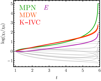
Figure 5: RG flow near $\nu=0$. RG flow of the quantities $\log(\chi(t)/\chi(0))$, where $\chi(t)$ is an order parameter susceptibility, for the 18 distinct order parameter structures with initial conditions $g_{o}=v_{z}=0.25$, and $N_{f}=8$, $\mu=0$ as appropriate for the vicinity of $\nu=0$. Moiré-polarised nematic (MPN) order is the leading instability, with moiré density wave and K-IVC closely contending at short RG times.

The fixed ray analysis is ‘unbiased’ – it makes no assumption on the bare couplings. To complement this, we calculate an explicit RG flow which allows us to establish which order parameters are dominant given a physically motivated set of bare interaction couplings. Hence, in addition to the fixed rays of Table 3, we show an RG plot in Fig. 7 for $\nu=2$, i.e. we set $N_{f}=4$. We demonstrate the emergence of T-IVC order for purely repulsive interactions: taking $g_{o}=u_{z}=0.2$, $v_{z}=0.05$, $v_{x\tau}=0.12$, i.e. positive couplings, but with $v_{x\tau}>v_{z}$. We find that the competition between K-IVC and T-IVC is determined by the relative magnitude of $v_{x\tau}$ and $v_{z}$: when these couplings are approximately equal, the IVC orders are nearly degenerate, while increasing the bare value of $v_{x\tau}$ ($v_{z}$) tends to promote T-IVC (K-IVC).

As mentioned earlier, the polarised state MSLP_- is degenerate with T-IVC, as a result of $\cal C$-symmetry. Subleading to T-IVC and MSLP_- order are $E$ superconductivity, along with K-IVC, MPN₊ and $A_{2}$ superconductivity; these conclusions are true for a range of coupling values varied around the choice shown in Fig. 7.

Table 3: Dominant flavour-polarised order parameters at $\bm{\nu=2}$. We assume the time-reversal-symmetric flavour polarisation $\{\tau s\}=\{++,--\}$, with corresponding projection operator ${\cal P}=(\tau_{0}s_{0}+\tau_{z}s_{z})/2$. We define an isovalley quantum number $\gamma=\tau=s$ as described in the main text; working in this basis automatically implements the flavour-projection. Due to projection, for $\nu=2$ the point group and TRS have a different representation than at $\nu=0$.

	Name	Abbreviation	Order Parameter	IR of $D^{s}_{6}$	IR of $D^{s}_{3}$	$\lambda_{j}$
IVC	$\Theta$-odd intervalley coherent	K-IVC	$\sigma_{x}\eta_{y}(\gamma_{x},\gamma_{y})$	$B_{2},A_{2}$	$A_{2}$	$\lambda_{7}$
	$\Theta$-even intervalley coherent	T-IVC	$\sigma_{x}\eta_{x}(\gamma_{x},\gamma_{y})$	$B_{1},A_{1}$	$A_{1}$	$\lambda_{8}$
polarised	$\Theta$-odd moiré-valley, sublattice polarised	MSLP-	$\sigma_{z}\eta_{z}\gamma_{z}$	$B_{1}$	$A_{1}$	$\lambda_{8}$
	$\Theta$-even moiré-valley, sublattice polarised	MSLP+	$\sigma_{z}\eta_{z}$	$A_{1}$	$A_{1}$	$\lambda_{11}$
	$\Theta$-even sublattice polarised	SLP+	$\sigma_{z}$	$A_{2}$	$A_{2}$	$\lambda_{7}$
	$\Theta$-odd sublattice polarised	SLP-	$\sigma_{z}\gamma_{z}$	$B_{2}$	$A_{2}$	$\lambda_{12}$
DW	$\Theta$-odd moiré density wave	MDW-	$(\gamma_{z}\eta_{x},\eta_{y})$	$-$	$E$	$\lambda_{9}$
$Q=0$	$A_{2}$ intervalley	$A_{2}$-SC	$\eta_{z}\gamma_{y}$	$A_{2}$	$A_{2}$	$\tilde{\lambda}_{5}$
	$A_{1}$ intervalley	$A_{1}$-SC	$\gamma_{y}$	$A_{1}$	$A_{1}$	$\tilde{\lambda}_{6}$
$Q\neq 0$	$E$  intervalley	$E$-QM-SC	$\sigma_{z}(\eta_{x},\eta_{y}\gamma_{z})\gamma_{y}$	$-$	$E$	$\tilde{\lambda}_{4}$
	$A_{2}$ intravalley	$A_{2}$-Q-SC	$\sigma_{y}\eta_{x}$	$A_{2}$	$A_{2}$	$\tilde{\lambda}_{5}$
	$B_{2}$ intravalley	$B_{2}$-Q-SC	$\sigma_{y}\eta_{x}\gamma_{z}$	$B_{2}$	$A_{2}$	$\tilde{\lambda}_{5}$

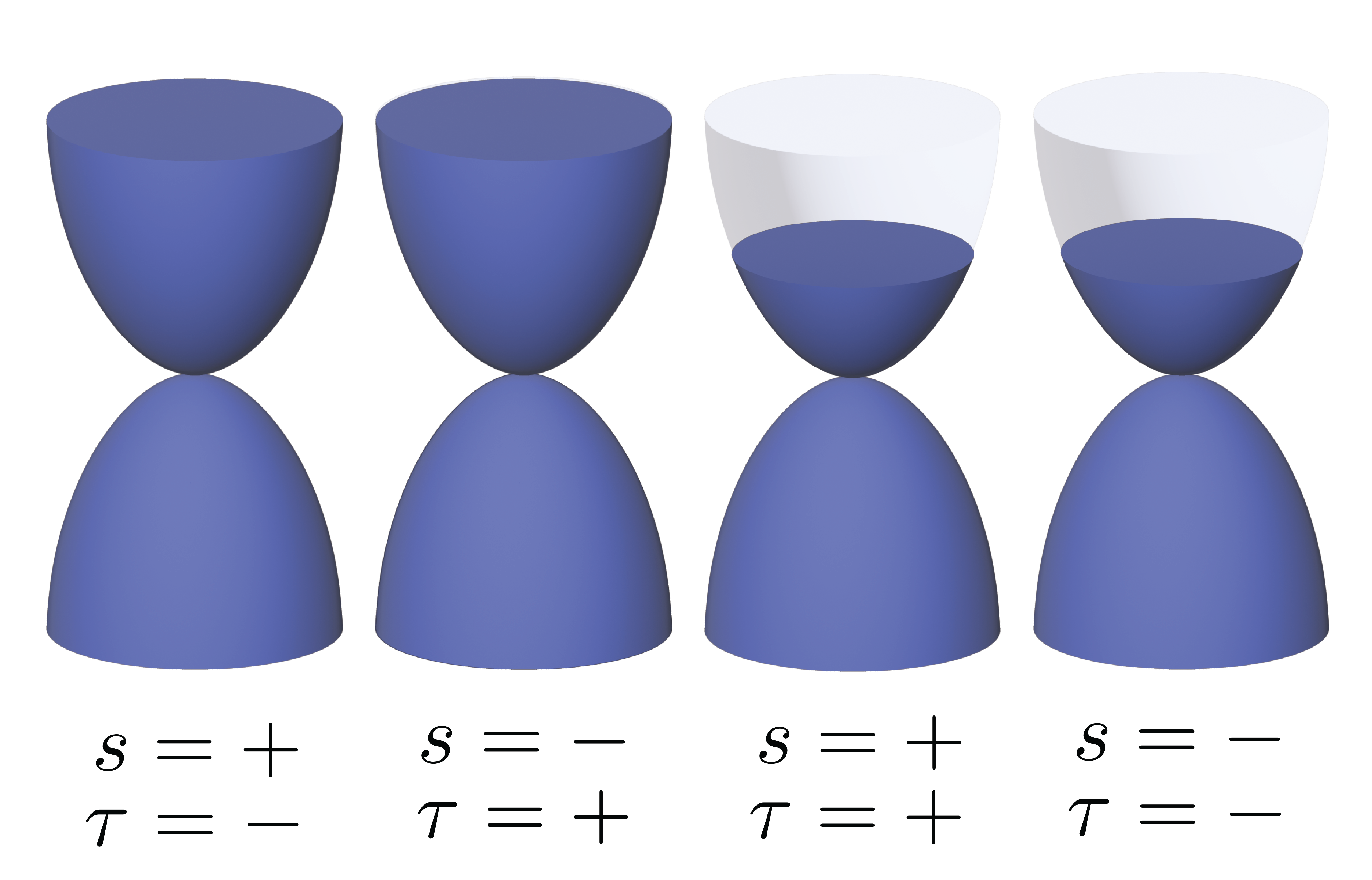
Figure 6: Flavour polarisation at $\bm{\nu=2}$. Experimental evidence suggests the remaining flavours after the Dirac revival at $\nu=2$ consist of opposite spins at opposite valleys.

Previous studies based on Hartree-Fock treatments and perturbation theory around the flat-band limit in twisted bilayer Bultinck2020 ; Bernevig2021d and trilayer graphene Christos2022 ; BernevigTrilayer ; TBorNotTB have led to the conventional wisdom that Coulomb interactions should favour K-IVC over T-IVC order – with the T-IVC state estimated to be significantly higher in energy ($\sim 5$ meV) than K-IVC order Bultinck2020 ; Christos2022 . It has been proposed that phonon-mediated attractive interactions combined with spin-valley polarisation can promote T-IVC PhononsTIVC , though T- and K-IVC remain close contenders. The RG flow enhances T-IVC, demonstrating that repulsive electronic interactions, without phonons, can allow T-IVC to dominate K-IVC order. We reiterate that recent STM studies of the spatial texture of the insulating state near $\nu=2$ see T-IVC order in low-strain devices Nuckolls2023 ; Kim2023 – our results provide a natural resolution of this puzzle.

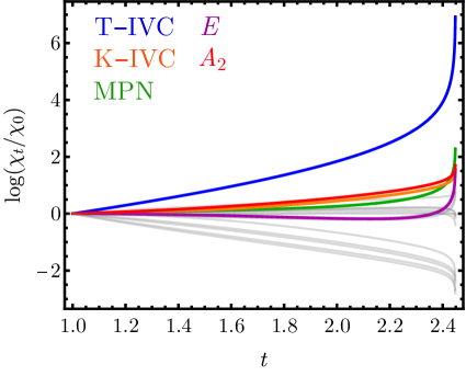
Figure 7: RG flow near $\nu=2$. RG flow of the quantities $\log(\chi(t)/\chi(0))$, where $\chi(t)$ is an order parameter susceptibility, for the 18 distinct order parameter structures with initial conditions $g_{o}=u_{z}=0.2$, $v_{z}=0.05$, $v_{x\tau}=0.12$, and $N_{f}=4$, $\mu=0$ as appropriate for the vicinity of $\nu=2$. T-IVC order dominates with a subleading $E_{2}$ superconducting instability; moiré-polarised nematic order and $A_{2}$ superconductivity appear as subleading competitors.

Upon doping away from the band touching point, so that $\nu\gtrsim 2$, the leading superconducting instabilities are the $E$ states, with $A_{2}$ appearing as a close competitor. While $E$/$E_{1,2}$ are the leading instabilities, as already noted they are finite momentum states and so may be more susceptible to disorder than $A_{2}$. The presence of $A_{2}$ superconductivity can resolve a second experimental puzzle, related to tunnelling conductance measurements Oh2021 ; Kim2022b ; Park2021c of the superconducting state near $\nu=2$ which show a ‘U-shaped’ density of states attributed to a full superconducting gap, that can become ‘V-shaped’ upon doping – typically attributed to gap nodes (aside from thermal fluctuations as a possible origin Fluctuations ). Since the $A_{2}$ state is odd under $C_{2x}$, the gap function has opposite signs at the two moiré valleys and vanishes at the $C_{2x}$-invariant $\Gamma M$ line in the Brillouin zone. While our theory becomes increasingly unjustified as doping is increased away from the Dirac point, if we assume that the superconducting order does not undergo a phase transition to a different irrep then the gap closes as the nodal lines of the $A_{2}$ state approach the Fermi level, which may explain the observed tunnelling conductance. Furthermore, we expect that the symmetry-imposed sign change of the $A_{2}$ intervalley state can also lead to subgap peaks as seen in tunnelling experiments in the strong-coupling limit Kim2022b ; CruzStronCoupl . However, we leave a quantitative analysis of this aspect to future work.

V.4 $\nu=1,3$

We will now describe the differences between the leading order parameters observed at $\nu=1$ and $3$. The simplest case is the region $3\leq\nu<4$, in which the Dirac revival has necessarily polarised all but one flavour, i.e. only a single species of spin and a single species of valley remain. Letting the remaining flavour be $\{s\tau\}=++$, the associated projection operator is $\mathcal{P}_{f}^{\nu=3}=(s_{0}+s_{z})(\tau_{0}+\tau_{z})/4$. After projection there are only two insulating states which appear, $\sigma_{z}\mathcal{P}^{\nu=3}_{f}$ and $\sigma_{z}\eta_{z}\mathcal{P}^{\nu=3}_{f}$, which have Chern numbers $\pm 1$ and 0 respectively – both of which have been seen in experiment near $\nu=3$ Pierce2021 . Any possible superconducting state is necessarily intra-flavour; the possible fixed-ray superconducting states significantly reduce to $\Delta_{5,\tau\tau}=(\sigma_{y}\eta_{x})\mathcal{P}^{\nu=3}_{f}$ , i.e. an $A_{2}$ $Q\neq 0$ superconductor. To the best of our knowledge, superconductivity has been observed near $\nu=0,1,2$ but not $\nu=3$ – consistent with the theoretical fragility of this state, though we speculate it may be observable in low-disorder devices endnote9 .

Near $\nu=1$, the projection operator may, without loss of generality, be written as $\mathcal{P}_{f}^{\nu=1}=s_{0}\tau_{0}-(s_{0}-s_{z})(\tau_{0}+\tau_{z})/4$, i.e. we project out the flavour $\{s\tau\}=+-$. The formation of an IVC state at $\nu\gtrsim 1$ leaves one flavour ungapped, which means a fully gapped state near either $\nu=1,3$ requires an order parameter $\propto\sigma_{z}$. We speculate that the states $\propto\sigma_{z}$ are more fragile to disorder, as experimental studies have seen a gap at $\nu=1,3$ mainly in low-disorder devices; further, many studies have found these insulating states do not appear in transport, but do appear in local compressibility measurements – suggesting the formation of local regions in which the insulating state forms, but which are shorted due to disorder-induced conductive channels Pierce2021 .

VI Wess-Zumino-Witten terms

Having described the ordering instabilities of the Dirac theory, we now consider the interplay of the insulating and superconducting states. A direct second-order transition between certain insulating and superconducting states is possible when the Landau-Ginzburg free energy possesses a so-called Wess-Zumino-Witten (WZW) term – a scenario which has been recently discussed in several studies on graphene-based systems GroverSenthil ; Shubhayu ; Khalaf2020sciadv ; Christos2020 ; Shubhayu2 ; Yveskyrm .

The presence of this term results in the skyrmion defects of a three-component particle-hole order parameter $\bm{m}$ carrying charge $2\mathcal{N}e$ with $\mathcal{N}\in\mathbb{N}$, so that the proliferation of vortices – and the associated destruction of the particle-hole order – leads to superconductivity GroverSenthil . Conversely, superconducting vortices carry the quantum numbers of the associated particle-hole order. We emphasise that our mechanism for superconductivity is a Fermi liquid instability via the RG-enhanced Coulomb interaction, arising from the quadratic Dirac dispersion – our analysis of skyrmion defects in the insulating phases will serve to demonstrate that continuous transitions between our superconducting and insulating phases are possible.

The WZW term can be written explicitly by defining $\bm{n}=(m_{1},m_{2},m_{3},\text{Re}\Delta,\text{Im}\Delta)$, and adding an auxiliary dimension $u$ to the spacetime dimensions $(\tau,x,y,z)$:

$$\mathcal{S}_{\text{WZW}} = i\frac{2\pi\mathcal{N}}{\Omega_{4}}\int_{0}^{1}du\int d\tau dxdy\sum_{abcde=1}^{5}\epsilon_{abcde}$$ (68)

$$~{}~{}~{}~{}~{}~{}~{}~{}~{}~{}\times n_{a}\partial_{u}n_{b}\partial_{\tau}n_{c}\partial_{x}n_{d}\partial_{y}n_{e}\,,$$

where $\Omega_{4}=8\pi^{2}/3$. The general criterion for the emergence of a WZW term in TBG as well as all possible compatible choices of $\bm{m}$ and zero-momentum superconducting order parameters have been worked out in Ref. Christos2020 , which we will next apply to our results (we present further details in the Supplemental Material).

We first note that there is no single set of particle-hole and superconducting orders among the fixed rays for the region $0\leq\nu<1$ around CNP consistent with a WZW term. This results from the fact that there is only one possible fixed-ray eigenvalue ($\tilde{\lambda}_{4}$) associated with superconductivity in this filling range, see Table 2, and the associated superconducting order parameters in Table 1 are all inconsistent with a WZW term. This observation might provide another reason for why superconductivity is less commonly observed for $|\nu|<1$ in experiment.

Moving on to $\nu=2$, our RG-dominant $E$ intervalley superconductor does not allow for a skyrmion-mediated transition, however the closely competing and less fragile $A_{2}$ state does. Most importantly, a WZW term between the $A_{2}$ intervalley superconductor, the two components of T-IVC order, and SLP₊ is possible. This is the most plausible scenario for a skyrmion-mediated critical point within our analysis, though we note that the SLP₊ is not close in energy to the T-IVC state within the RG without fine-tuning of parameters. Apart from this, the only other WZW term we find is the one between the $A_{1}$ intervalley superconductor, K-IVC, and SLP₊ order – the scenario of Ref. Khalaf2020sciadv . Our conclusions are that superconducting vortices in our primary candidate superconductor, the $A_{2}$ intervalley state, can carry quanta of the T-IVC GroverSenthil ; they could therefore exhibit a Kekulé pattern similar to that seen in STM analysis of superconducting state near $\nu=2$ Nuckolls2023 . The analysis further shows that the transition from T-IVC to $A_{2}$ superconductivity may be second order.

VII Discussion

We have argued that TBG near integer fillings is described by a Dirac theory as a result of the observed revivals, with the assumption that the Fermi velocity is small enough that the fermions have a quadratic dispersion in some range of momenta near the Dirac points. The result is a non trivial renormalisation group flow across an associated window of temperatures: the particle-hole fluctuations near the band touching points result in nematic and insulating states, while doping away from the band-touching results in superconductivity dominating. Our theory is able to simultaneously describe both the insulating and superconducting states, a major advantage over alternative methods such as Hartree-Fock Guinea2018 ; Bultinck2020 ; Bernevig2021d ; Bernevig2021e ; Kwan2021b ; Liu2021c ; Liu2021b ; PhononsTIVC ; Wagner2022 ; Christos2022 . We motivated our assumption of a quadratic energy regime by appealing to an approximate particle-hole symmetry TBG possesses, however a direct verification of the physical values of $v$ and $\beta$ is experimentally feasible, via measurements of the electronic compressibility shahal .

The theory can explain a great deal of the observed phenomena in TBG. Firstly, the theory provides a unified explanation of the phase diagram of TBG throughout the entire region $-4<\nu<4$, which consists of interlaced insulating/nematic and superconducting states. The theory explains why insulating/nematic states appear near each integer filling, and why superconducting states have been observed in the absence of insulating states – the phases have a common origin, rather than a ‘parent-child’ relationship. Furthermore, the theory naturally accounts for a gapped CNP in low-strain devices and a gapless nematic CNP in the presence of strain, consistent with experiment, and can account for the sequence of Chern numbers associated to the insulating states near integer filling.

Secondly, recent STM studies of the insulating states near $\nu=2$ have found evidence of T-IVC order in low-strain devices Nuckolls2023 ; Kim2023 ;. Prior mean-field treatments and strong-coupling calculations with Coulomb interactions have favoured the K-IVC state over T-IVC (see, e.g., Bultinck2020 ; Bernevig2021d ; Christos2022 ; BernevigTrilayer ; TBorNotTB ), but here we find that RG provides a mechanism for the appearance of T-IVC order, relying on repulsive interactions rather than a resort to phonons. The T-IVC state exhibits a spatial pattern known as a Kekulé distortion, and in the presence of strain can result in a spatial texture known as an ‘incommensurate Kekulé spiral’ (IKS) – a state introduced in Ref. Kwan2021 , which Nuckolls2023 ; Kim2023 also observed in strained devices.

Thirdly, our results suggest a resolution of another recent experimental puzzle. Tunnelling conductance measurements of the superconducting state near $|\nu|=2$ show a transition from a V-shaped density of states to a U-shaped density of states as a function of doping Oh2021 ; Kim2022b ; Park2021c , indicating a transition between nodal and fully-gapped superconductivity. Our prediction of $A_{2}$ superconductivity in the Dirac theory near $|\nu|=2$ provides a possible microscopic mechanism which naturally accounts for these features. Note that the U-shaped regime has only been reported in tTLG, however it is generally believed that this system shares the same pairing symmetry as TBG.

Fourthly, our proposed link between revivals and superconductivity can explain the asymmetry of the phase diagram between electron- $\nu>0$ and hole- $\nu<0$ doping. Experiments have observed that that the Dirac revivals appear in a different window of angles for $\nu>0$ and $\nu<0$ – e.g. Ref. Polski2022 observed revivals for $\nu>0$ in the range $\theta\approx 0.88^{\circ}-1.04^{\circ}$, but observed revivals for $\nu<0$ in the range $\theta\approx 0.97^{\circ}-1.23^{\circ}$ endnote10 . In our theory, the Dirac revivals create the parent state from which superconductivity emerges at low temperatures – i.e. the quadratic momentum regime near the Dirac point – consistent with the observed asymmetry in the superconducting phase diagram.

Fifthly, the Dirac revival picture also offers two possible explanations of why the superconducting states at $\nu=0,1,3$ appear to be less robust – firstly that the leading superconducting orders which appear are finite momentum states fragile to disorder, and secondly that the Dirac revival does not always appear at $|\nu|=1,3$.

Finally, the theory explains why superconductivity is generally absent when TBG is aligned with an hBN substrate, which breaks $C_{2z}$ symmetry and gaps out the Dirac points, obviating the interaction physics of the band-touching point.

A host of other moiré systems – including twisted multi-layer graphene and twisted transition metal dichalcogenides – are characterised by Dirac particles near charge neutrality with flattened dispersions. Our RG results open up a possible approach to studying the interaction physics of these systems – in fact, experiments on twisted trilayer graphene also indicate signatures of Dirac revivals at integer fillings Park2021a ; Hao2021 ; Cao2021a ; Siriviboon2021 , as well as multi-layer graphene proximitised with WSe₂ Zhang2021b , so we anticipate the physics of quadratic Dirac fermions is directly relevant in these systems as well. Moreover, Bernal-stacked bilayer graphene proximitised with WSe₂ – recently found to exhibit superconductivity Zhang2023 – also possesses a flavour-polarised Fermi surface characterised by a spin-valley locking equivalent to our scenario for TBG near $|\nu|=2$. Our analysis suggests that flavour polarisation and band-touching Dirac states are the essential ingredient in the emergence of insulating and proximate superconducting states in these systems.

Supplementary Material

S1 Symmetry analysis

S1.1 Continuum model

The twisted bilayer may be described via an effective continuum Hamiltonian, valid at long-wavelengths compared to the lattice spacing of graphene. Two monolayers, each with linear dispersion near the $K$-points, are coupled due to interlayer tunnelling; the Bistritzer-MacDonald (BM) Hamiltonian is given by $H=H_{0}+V$ where

$$H_{0} =\int d^{2}\bm{r}\sum_{\ell}\psi_{\ell}^{\dagger}(\bm{r})e^{-i\tau_{z}{\sigma_{z}\ell}\theta/2}v(\tau_{z}\sigma_{x}(-i\partial_{x})+\sigma_{y}(-i\partial_{y}))\psi_{\ell}(\bm{r})+\sum_{j,{\ell<\ell^{\prime}}}e^{i{\tau_{z}}\bm{G}_{j}\cdot\bm{r}}\psi^{\dagger}_{\ell}(\bm{r})T^{j}\psi_{\ell^{\prime}}(\bm{r})+\text{h.c.}$$ (S1)

$$\equiv\int d^{2}\bm{r}\sum_{\ell,\ell^{\prime}}\psi_{\ell}^{\dagger}\left[h_{0}(\bm{r})\ell_{0}+h_{T}(\bm{r})\ell_{-}+h_{T}^{\dagger}(\bm{r})\ell_{+}\right]_{\ell,\ell^{\prime}}\psi_{\ell^{\prime}}$$

with the monolayer and tunnelling Hamiltonians,

$$h_{0}(\bm{r}) =e^{-i\tau_{z}{\sigma_{z}\ell_{z}}\theta/2}v(\tau_{z}\sigma_{x}(-i\partial_{x})+\sigma_{y}(-i\partial_{y}))$$ (S2)

$$h_{T}(\bm{r}) =e^{i{\tau_{z}}\bm{G}_{j}\cdot\bm{r}}T^{j}$$ (S3)

where $(\psi^{\dagger}_{\ell}(\bm{r}))_{\tau,\sigma,s}=\psi^{\dagger}_{\ell,\tau,\sigma,s}$ for $\ell=\pm$ corresponding to separate layers, is an eight-component spinor with monolayer valley ($\tau$), sublattice pseudospin ($\sigma$) and spin ($s$) degrees of freedom. We have also used Pauli matrices $\ell_{0}$, $\ell_{\pm}=(\ell_{x}\pm i\ell_{y})/2$ and $\ell_{z}$. The tunnelling matrices coupling the two layers $T^{j}$ are given by

$$T^{j}_{\sigma\sigma^{\prime}}=\left(\begin{array}[]{cc}w_{0}e^{-\frac{2\pi i}{3}j\tau_{z}}&w_{1}e^{\frac{2\pi i}{3}j\tau_{z}}\\ w_{1}&w_{0}e^{-\frac{2\pi i}{3}j\tau_{z}}\end{array}\right)_{\sigma\sigma^{\prime}}$$ (S6)

with tunnelling constants $w_{0}$ and $w_{1}$, index $j=\{0,\pm 1\}$ and moiré wavevectors $\bm{G}_{j}=(8\pi/3)\sin(\theta/2)R_{\phi_{j}}(0,-1)$, with $R_{\phi_{j}}$ is an in-plane rotation through an angle $\phi_{j}=0,2\pi/3,-2\pi/3$. The Coulomb interaction is

$$V=\tfrac{1}{2}\int d^{2}\bm{r}d^{2}\bm{r}^{\prime}\sum_{\ell,\ell^{\prime}}V(\bm{r}-\bm{r}^{\prime})\psi^{\dagger}_{\ell}(\bm{r})\psi_{\ell}(\bm{r})\psi^{\dagger}_{\ell^{\prime}}(\bm{r}^{\prime})\psi_{\ell^{\prime}}(\bm{r}^{\prime})$$ (S7)

where the precise form of the screened Coulomb potential $V(\bm{r}-\bm{r}^{\prime})$ shall be discussed later in this Supplement. The spatial modulation of the interlayer coupling results in the formation of a mini Brillouin zone corresponding to a triangular superlattice with spacing $L=a/(2\sin(\theta/2))$. For small $\theta$, $L\gg a$ which justifies the continuum approximation.

S1.2 Symmetries of the continuum model

The bilayer satisfies threefold rotational symmetry in the plane, $C_{3z}\psi^{\dagger}_{\ell,\tau,\sigma,s}(\bm{r})C^{-1}_{3z}=e^{\frac{\pi i}{3}\tau(\sigma-\ell)}\psi^{\dagger}_{\ell,\tau,\sigma,s}(C_{3z}^{-1}\bm{r})$, twofold rotational symmetry about the $x$ axis, $C_{2x}\psi^{\dagger}_{\ell,\tau,\sigma,s}(x,y)C_{2x}^{-1}=\psi^{\dagger}_{\bar{\ell},\tau,\bar{\sigma},s}(x,-y)$, as well as a twofold rotational symmetry in the plane $C_{2z}\psi^{\dagger}_{\ell,\tau,\sigma,s}(\bm{r})C_{2z}^{-1}=\psi^{\dagger}_{\ell,\bar{\tau},\bar{\sigma},s}(\bm{D-r})$ with $\bm{D}=(L/(\sqrt{3}),0)$. The system maintains an SU(2) spin rotational symmetry due to absence of spin-orbit coupling, which we may combine with physical time-reversal symmetry to introduce a spin-independent time-reversal operation $\Theta$ satisfying $\Theta\psi^{\dagger}_{\ell,\tau,\sigma,s}(\bm{r})\Theta^{-1}=\psi^{\dagger}_{\ell,\bar{\tau},\sigma,s}(\bm{r})$. In addition to the point group symmetries and time-reversal, the continuum model possesses an SU(2) $\times$ SU(2) symmetry corresponding to independent spin rotations in the two valleys. This symmetry is broken by interactions – specifically, the weak but finite intervalley Hund’s coupling $J_{H}$ – but in our analysis we neglect such terms, and so the SU(2) $\times$ SU(2) symmetry is exact.

In addition to the above symmetries, which hold for the BM model as printed in (S1), for the analysis in the main text we work solely in the PH symmetric limit, i.e. taking $e^{-i\tau_{z}{\sigma_{z}\ell}\theta/2}\approx 1$. For convenience we explicitly state the PH-symmetric BM model,

$$h(\bm{r})=h_{0}(\bm{r})\ell_{0}+\sum_{j}h_{T}(\bm{r})\ell_{-}+\text{h.c.}$$ (S8)

$$h_{0}(\bm{r})=v(\tau_{z}\sigma_{x}(-i\partial_{x})+\sigma_{y}(-i\partial_{y}))$$ (S9)

$$h_{T}(\bm{r})=e^{i{\tau_{z}}\bm{G}_{j}\cdot\bm{r}}T^{j}$$ (S10)

Then it is straightforwardly checked that ${\cal P}\tilde{h}(\bm{k}){\cal P}^{\dagger}=\tilde{h}(-\bm{k})$ for PH anti-unitary operator ${\cal P}=\sigma_{x}\ell_{y}K$, where the Fourier transform of $h(\bm{r})$ is denoted $\tilde{h}(\bm{k})$

S1.3 Relation to the Dirac theory

As discussed in the main text, we can index the states at the Dirac points using a basis of eight orbital states $|\sigma,\tau,\eta\rangle=|\sigma\rangle\otimes|\tau\rangle\otimes|\eta\rangle$ with $\sigma=\pm$ indexing the twofold degenerate states at the same minivalley. The $\eta$-index is chosen such that in the limit of decoupled layers (zero tunnelling) $e^{i\bm{k}\cdot\bm{r}}|\sigma,\tau,\eta\rangle\to e^{i\bm{k}\cdot\bm{r}}|\sigma,\tau,\ell\rangle$, where $\bm{k}$ is measured from the valley momentum $\bm{K}_{\ell}$ of the layer $\ell$. At this high symmetry point $|\sigma,\tau,\eta\rangle$ and $|\sigma,\tau,\ell\rangle$ have identical transformation properties under $D_{6}$ and $\Theta$. Turning on tunnelling between layers changes the relationship between $|\sigma,\tau,\eta\rangle$ and $|\sigma,\tau,\ell\rangle$, but since $D_{6}$ and $\Theta$ remain symmetries of the model, it does not change the transformation properties of $|\sigma,\tau,\eta\rangle$.

S1.4 Symmetry representations in the Dirac theory

S1.4.1 $\nu=0$

Considering only the spinless transformations, the action of the $D_{6}$ group is represented by the unitary operators

$$C_{2z}: \quad U_{C_{2z}}=\tau_{x}\sigma_{x}$$ (S11)

$$C_{2x}: \quad U_{C_{2x}}=\eta_{x}\sigma_{x}$$ (S12)

$$C_{3z}: \quad U_{C_{3z}}=e^{i\pi\tau_{z}(\sigma_{z}-\eta_{z})/3}$$ (S13)

here $\tau_{\mu},\eta_{\mu},\sigma_{\mu}$ are Pauli matrices acting on graphene valley, moiré valley and sublattice indices. In addition, there are non-spatial symmetries

$$\text{(TRS)}\quad\Theta =\tau_{x}K,$$ (S14)

$$\text{(PHS)}\quad{\cal P} =\sigma_{x}\eta_{y}K,\quad({\cal P}^{2}=-1)$$ (S15)

$$\text{(Chiral)}\quad{\cal S} ={\cal P}\Theta=\sigma_{x}\eta_{y}\tau_{x}$$ (S16)

$$\quad{\cal C} =-i\sigma_{z}{\cal S}=\sigma_{y}\eta_{y}\tau_{x}.$$ (S17)

where $K$ denotes complex conjugation. Note that ${\cal C}$ is an emergent, low-energy symmetry, see the discussion in Sec S1.5. For convenience, we present the transformation laws of bilinears in Table S1.

S1.4.2 $\nu=2$

Considering transformations of the spin-valley locked system near $\nu=2$, we construct the following representation of spinful $D_{6}^{s}$ and TRS,

$$C_{2z}^{\prime}: \quad U_{C_{2z}}=i\gamma_{x}\sigma_{x}$$ (S18)

$$C_{2x}^{\prime}: \quad U_{C_{2x}}=\eta_{x}\sigma_{x}$$ (S19)

$$C_{3z}^{\prime}: \quad U_{C_{3z}}=e^{i\pi\gamma_{z}(\sigma_{z}-\eta_{z})/3}$$ (S20)

$$\Theta^{\prime}: \quad\Theta=i\gamma_{y}K.$$ (S21)

Here $\gamma_{\mu}$ acts on the spin-valley locked index $\gamma=s=\tau$. We use this representation in Table 3.

Table S1: Transformation laws for relevant bilinears.

	$C_{3z}$	$C_{2x}$	$C_{2z}$	$\Theta$	${\cal P}$	${\cal C}$
$q_{\pm}$	$q_{\pm}e^{\pm\frac{2\pi i}{3}}$	$q_{\mp}$	$-q_{\pm}$	$-q_{\mp}$	$-q_{\mp}$	$q_{\mp}$
$q_{\pm}^{2}$	$q_{\pm}^{2}$ $e^{\pm\frac{4\pi i}{3}}$	$q_{\mp}^{2}$	$q_{\pm}^{2}$	$q_{\pm}^{2}$	$q_{\pm}^{2}$	$q_{\pm}^{2}$
$q_{\pm}^{3}$	$q_{\pm}^{3}$	$q_{\mp}^{3}$	$-q_{\pm}^{3}$	$-q_{\mp}^{3}$	$-q_{\mp}^{3}$	$q_{\mp}^{3}$
$\alpha_{\pm}$	$e^{\pm\frac{2\pi i}{3}}$ $\alpha_{\pm}$	$\alpha_{\mp}$	$\alpha_{\pm}$	$\alpha_{\mp}$	$\alpha_{\pm}$	$-\alpha_{\pm}$
$\tau_{z}$	$\tau_{z}$	$\tau_{z}$	$-\tau_{z}$	$-\tau_{z}$	$\tau_{z}$	$-\tau_{z}$
$\eta_{z}$	$\eta_{z}$	$-\eta_{z}$	$\eta_{z}$	$\eta_{z}$	$-\eta_{z}$	$-\eta_{z}$
$\sigma_{z}$	$\sigma_{z}$	$-\sigma_{z}$	$-\sigma{z}$	$\sigma_{z}$	$-\sigma_{z}$	$-\sigma_{z}$

S1.5 Effective Dirac Hamiltonian

From the transformation properties of the $\sigma$ matrices and products of $\tau_{z},\eta_{z},\sigma_{z}$ in Table S1 we can construct the single particle Hamiltonian order by order in $q$; the result is the most general single-particle Hamiltonian permitted by symmetry for the Dirac states. Since no $q$-independent operators are invariant under all symmetries, the Hamiltonian must vanish at $q=0$. Using the constraints of $D_{6}$ and $\Theta$, one finds

$$\mathcal{H}_{0}=v\tau_{z}(e^{i\phi_{1}\eta_{z}}k_{-}\alpha_{+}+e^{-i\phi_{1}\eta_{z}}k_{+}\alpha_{-})+\beta(e^{i\phi_{2}\eta_{z}}k_{+}^{2}\alpha_{+}+e^{-i\phi_{2}\eta_{z}}k_{-}^{2}\alpha_{-})+\beta^{\prime}k^{2}\alpha_{0}$$

$$+\,\gamma_{1}\left(e^{i\phi_{3}\eta_{z}}k_{+}^{3}+e^{-i\phi_{3}\eta_{z}}k_{-}^{3}\right)+\gamma_{2}\tau_{z}k^{2}\left(e^{i\phi_{4}\eta_{z}}k_{+}\alpha_{-}+e^{-i\phi_{4}\eta_{z}}k_{-}\alpha_{+}\right)+...$$ (S32)

Further, the $\eta$-dependent phases can be fixed using the constraints of ${\cal S}={\cal P}{\cal T}$; the effective Dirac Hamiltonian, up to quadratic-order in $\bm{k}$, is

$$\mathcal{H}_{0}=v\tau_{z}(k_{+}\alpha_{-}+k_{-}\alpha_{+})+i\beta\eta_{z}\left(k_{+}^{2}\alpha_{+}-k_{-}^{2}\alpha_{-}\right).$$ (S33)

As explained in the main text, this low-energy model hosts an emergent symmetry $[{\cal C},\mathcal{H}_{0}]=0$, with ${\cal C}=-i\sigma_{z}{\cal S}$. This emergent symmetry only holds in the infrared – the first term which breaks this ${\cal C}$-symmetry occur at cubic-order in $\bm{k}$, i.e.

$$\delta\mathcal{H}_{0}=\gamma\tau_{z}(k_{+}^{3}+k_{-}^{3}).$$ (S34)

Hence, the effective theory close to the Dirac points acquires the approximate emergent symmetry ${\cal C}$ in addition to ${\cal S}$, $D_{6}$ and ${\cal T}$.

S1.6 Interacting Hamiltonian

We now consider the Coulomb interaction. In proximity to metallic gates, the $2d$ Coulomb potential reads

$$V(\bm{q})=\tfrac{2\pi e^{2}}{\varepsilon_{r}q}\tanh(qD)$$ (S35)

where $D$ is the distance to the adjacent gates symmetrically spaced above and below the device. The interaction at large $q$ is $\propto 1/q$ and is unscreened by gates, and saturates to $\sim 2\pi e^{2}D/\varepsilon_{r}$ for $q<1/D$. In our analysis, we will neglect the long-range momentum dependence $\propto 1/q$ of the Coulomb interactions

We will also restrict our attention to interactions involving momenta at the Dirac points which conserve $\tau$ – as we have discussed, monolayer valley is a good quantum number in TBG due to the large momentum transfer, relative to the moiré momentum scale $Q_{m}=(8\pi/3)\sin(\theta/2)$, required to scatter between valleys. We also neglect the momentum dependence of the interaction constants near the Dirac points; an extension of the RG analysis to include the long-range part of the Coulomb potential may be left for future work.

Using the symmetry representations of the previous sections, we may derive the symmetry-allowed form of the interactions in terms of symmetry-invariant products of fermion bilinears. For a real-valued potential which only depends on the spatial coordinates, only time-reversal-invariant bilinears are allowed Li2020 – a restriction widely unappreciated in the literature. This condition is lifted by the RG flow. A variation of the proof in Li2020 in the presence of the approximate particle-hole symmetry shows that similarly only $\mathcal{P}\Theta$-invariant bilinears are allowed to appear – and this criterion is not lifted by the RG flow. Since this symmetry is approximate, we shall begin by stating the full set of interactions allowed by $D_{6}$ and TRS, before indicating the $\mathcal{P}\Theta$-invariant subset.

The full set of interactions allowed by $D_{6}$ and $\Theta$ are

$$V=g_{o}\sigma_{0}\tau_{0}\eta_{0}\otimes\sigma_{0}\tau_{0}\eta_{0}+g_{x}(\sigma_{x}\tau_{0}\eta_{0}\otimes\sigma_{x}\tau_{0}\eta_{0}+\sigma_{y}\tau_{z}\eta_{0}\otimes\sigma_{y}\tau_{z}\eta_{0})+g_{z\tau}\sigma_{z}\tau_{0}\eta_{0}\otimes\sigma_{z}\tau_{0}\eta_{0}$$

$$+v_{o}(\sigma_{0}\tau_{0}\eta_{x}\otimes\sigma_{0}\tau_{0}\eta_{x}+\sigma_{0}\tau_{z}\eta_{y}\otimes\sigma_{0}\tau_{z}\eta_{y})+v_{x}(\sigma_{x}\tau_{0}\eta_{x}\otimes\sigma_{x}\tau_{0}\eta_{x}+\sigma_{x}\tau_{z}\eta_{y}\otimes\sigma_{x}\tau_{z}\eta_{y}+\sigma_{y}\tau_{0}\eta_{y}\otimes\sigma_{y}\tau_{0}\eta_{y}+\sigma_{y}\tau_{z}\eta_{x}\otimes\sigma_{y}\tau_{z}\eta_{x})$$

$$+v_{z}(\sigma_{z}\tau_{0}\eta_{x}\otimes\sigma_{z}\tau_{0}\eta_{x}+\sigma_{z}\tau_{z}\eta_{y}\otimes\sigma_{z}\tau_{z}\eta_{y})+iw(\sigma_{0}\tau_{0}\eta_{x}\otimes\sigma_{z}\tau_{z}\eta_{y}-\sigma_{0}\tau_{z}\eta_{y}\otimes\sigma_{z}\tau_{0}\eta_{x}+\sigma_{z}\tau_{z}\eta_{y}\otimes\sigma_{0}\tau_{0}\eta_{x}-\sigma_{z}\tau_{0}\eta_{x}\otimes\sigma_{0}\tau_{z}\eta_{y})$$

$$+u_{o}\sigma_{0}\tau_{0}\eta_{z}\otimes\sigma_{0}\tau_{0}\eta_{z}+u_{x}(\sigma_{y}\tau_{z}\eta_{z}\otimes\sigma_{y}\tau_{z}\eta_{z}+\sigma_{x}\tau_{0}\eta_{z}\otimes\sigma_{x}\tau_{0}\eta_{z})+u_{z}\sigma_{z}\tau_{0}\eta_{z}\otimes\sigma_{z}\tau_{0}\eta_{z}$$ (S36)

along with the set of interactions generated by $\Omega^{\mu}\in\{\sigma_{0}\tau_{0}\eta_{0},\sigma_{z}\tau_{0}\eta_{z},\sigma_{z}\tau_{0}\tilde{\eta}_{\pm}\}$, where $\Omega^{\mu}$ is a bilinear taken from the above set. This large set of interactions is the interacting Hamiltonian one must work with when particle-hole symmetry is relaxed, and we shall analyse it further in a future publication. As stated in the main text, if we insist on only including $\mathcal{P}\Theta$-invariant bilinears, along with bilinears that commute with the emergent ${\cal C}$ which applies near the Dirac point, this large set of interactions becomes remarkably constrained, including only three couplings

$$V=g_{o}(\sigma_{0}\tau_{0}\eta_{0}\otimes\sigma_{0}\tau_{0}\eta_{0})+v_{z}(\sigma_{z}\tau_{0}\tilde{\eta}_{\pm}\otimes\sigma_{z}\tau_{0}\tilde{\eta}_{\mp})+u_{z}(\sigma_{z}\tau_{0}\eta_{z}\otimes\sigma_{z}\tau_{0}\eta_{z}).$$ (S37)

where $\tilde{\eta}_{\pm}=\eta_{x}\pm i\tau_{z}\eta_{y}$, along with the set of interactions generated by $\Omega^{\mu}\in\{\sigma_{0}\tau_{0}\eta_{0},\sigma_{z}\tau_{0}\eta_{z},\sigma_{z}\tau_{0}\tilde{\eta}_{\pm}\}$, i.e. the interacting Hamiltonian presented in the main text.

S2 Quadratic Dirac fermions in the $\mathcal{P}$-symmetric Bistrizer-MacDondald Model

With the inclusion of lattice relaxation $w_{0}\neq w_{1}$, the continuum model Eq. (S1) does not generally possess a twist angle at which the Dirac velocity vanishes. However, it has been shown Raquel that the presence of particle-hole symmetry $\mathcal{P}$ in a Dirac system allows the velocity to be tuned to zero with a single parameter. Motivated by this observation, in this section we impose $\mathcal{P}$ as an exact symmetry, as described earlier, and compute the bandstructure as a function of twist angle and the ratio of tunnelling amplitudes $w_{0}/w_{1}$, while setting $w_{1}=0.097$ eV (following Ref. Koshino2018 ). We find for a range of $w_{0}$ and $w_{1}$, there always exists a twist angle $\theta_{Q}$ for which the dispersion is quadratic, i.e. the velocity vanishes and the second derivative of the dispersion is nonzero, see Fig. S1. See Ref. Raquel for the dependence of $v$ on twist angle in the $\mathbf{\mathcal{P}}$-symmetric continuum model.

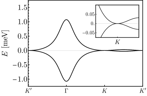
Figure S1: Quadratic band-touching in the $\mathbf{\mathcal{P}}$-symmetric continuum model. Left: bandstructure of the $\mathbf{\mathcal{P}}$-symmetric continuum model, with inset magnifying the dispersion near the moiré $K$-points, for $\theta=1.072^{\circ}$ and $w_{0}/w_{1}=0.74$. Right: a plot of the critical angle at which the dispersion is quadratic $\theta_{Q}$ against the ratio of tunnel couplings $w_{0}/w_{1}$. In both plots we have fixed $w_{1}=0.097$ eV.

S3 Analytic exact renormalisation group

S3.1 Wetterich equation

This appendix will describe the exact analytic RG formalism. We begin by deriving the Wetterich equation for a fermionic system Polchinski1984 ; Wetterich1993 . The derivation will closely follow Ref. Platt2013 . We have the generating functional

$$W[\bar{\eta},\eta]=\int D\psi D\bar{\psi}e^{-S[\bar{\psi},\psi]+\int\bar{\eta}\psi+\bar{\psi}\eta}$$ (S38)

and its logarithm,

$$\mathcal{G}[\bar{\eta},\eta]=-\log\left(W[\bar{\eta},\eta]\right)$$ (S39)

whose derivatives evaluated at $\bar{\eta}=\eta=0$ give the connected $n$-particle Green’s functions,

$$G_{1,...,n;1^{\prime},...,n^{\prime}}=-\frac{1}{Z}\int D\psi D\bar{\psi}\,e^{-S[\bar{\psi},\psi]}\ \psi_{1}...\psi_{n}\bar{\psi}_{1^{\prime}}...\bar{\psi}_{n^{\prime}}$$ (S40)

We employ DeWitt notation, in which each of the indices $i\in\{1,...,n;1^{\prime},...,n^{\prime}\}$ is shorthand for all quantum numbers: frequencies $\omega_{i}$, momentum $\bm{k}_{i}$, $\sigma_{i}$, $\tau_{i}$, $\eta_{i}$ and spin $s_{i}$. Integration over momentum and frequencies, as well as summation over pseudospin etc., all appear as summation over DeWitt indices. We shall also employ Einstein summation notation throughout. We seek to derive an exact flow equation for the generating functional, allowing us to circumvent performing the path integral. We write the action,

$$S[\bar{\psi},\psi]=-\bar{\psi}_{a}Q_{ab}\psi_{b}+U_{1234}\bar{\psi}_{1}\bar{\psi}_{2}\psi_{3}\psi_{4}$$ (S41)

and we make the replacement $Q_{ab}\rightarrow Q_{ab}^{\Lambda}$ where $Q_{ab}^{\Lambda}\rightarrow\infty$ as $\Lambda\rightarrow\infty$ and $Q_{ab}^{\Lambda}\rightarrow Q_{ab}=G^{-1}$ the inverse Green’s function as $\Lambda\rightarrow 0$. Accordingly, we obtain a cutoff-dependent generating functional $\mathcal{G}^{\Lambda}$ with the boundary conditions

$$\mathcal{G}^{\Lambda}=\begin{cases}\mathcal{G}&\text{for}\ \Lambda\rightarrow 0\\ 0&\text{for}\ \Lambda\rightarrow\infty\end{cases}$$ (S42)

Note that in $S[\bar{\psi},\psi]$, only the Green’s function $Q^{\Lambda}$ contains any $\Lambda$ dependence, but that is adequate to regularise the theory. We follow the trajectory $\mathcal{G}^{\Lambda}$ from the known starting point at large $\Lambda$ to the full functional at $\Lambda=0$. We determine the derivative $\partial_{\Lambda}\mathcal{G}^{\Lambda}$ and consider the extrapolation to $\Lambda\rightarrow 0$ as an initial value problem. To do this we replace the functional integration with a formally exact differential equation:

$$\partial_{\Lambda}\mathcal{G}^{\Lambda}[\bar{\eta},\eta] =-e^{\mathcal{G}^{\Lambda}[\bar{\eta},\eta]}\partial_{\Lambda}e^{-\mathcal{G}^{\Lambda}[\bar{\eta},\eta]}$$

$$=-e^{\mathcal{G}^{\Lambda}[\bar{\eta},\eta]}\int D\psi D\bar{\psi}\,\bar{\psi}_{a}\partial_{\Lambda}Q_{ab}\psi_{b}\,e^{-S[\bar{\psi},\psi]+\bar{\eta}\psi+\bar{\psi}\eta}$$

$$=\partial_{\Lambda}Q_{ab}\,(e^{\mathcal{G}^{\Lambda}[\bar{\eta},\eta]}\partial_{\eta_{a}}\partial_{\bar{\eta}_{b}}e^{-\mathcal{G}^{\Lambda}[\bar{\eta},\eta]})$$

$$=\partial_{\Lambda}Q_{ab}(\partial_{{\eta}_{a}}\mathcal{G}^{\Lambda}[\bar{\eta},\eta]\partial_{\bar{\eta}_{b}}\mathcal{G}^{\Lambda}[\bar{\eta},\eta]-\partial_{{\eta}_{a}}\partial_{\bar{\eta}_{b}}\mathcal{G}^{\Lambda}[\bar{\eta},\eta])$$ (S43)

Upon Taylor expanding the functional $\mathcal{G}^{\Lambda}[\bar{\eta},\eta]$, the last line gives us an infinite hierarchy of differential equations for the Taylor coefficients, namely the connected Green’s functions. The result is the so-called Polchinski equation. In practice, it is more convenient to write this equation in terms of the Legendre transform of the generating functional, namely the effective action $\Gamma^{\Lambda}[\bar{\zeta},\zeta]$,

$$\Gamma^{\Lambda}[\bar{\zeta},\zeta]=\mathcal{G}^{\Lambda}[\bar{\eta},\eta]+\bar{\eta}_{a}\zeta_{a}+\bar{\zeta}_{b}\eta_{b}$$ (S44)

where the conjugate fields are defined as

$$\zeta_{a}=-\partial_{\bar{\eta}_{a}}\mathcal{G}^{\Lambda},\ \ \ \ \ \ \ \ \ \ \bar{\zeta}_{a}=\partial_{\eta_{a}}\mathcal{G}^{\Lambda}$$ (S45)

The 1PI vertex functions are the $\zeta$ derivatives of the effective action, ie

$$V^{\Lambda}_{1,...,n;1^{\prime},...,n^{\prime}}=\frac{\partial^{(2n)}\Gamma^{\Lambda}[\bar{\zeta},\zeta]}{\partial\bar{\zeta}_{1}...\partial\bar{\zeta}_{n}\partial\zeta_{1^{\prime}}...\partial\zeta_{n^{\prime}}}\Big{\rvert}_{\zeta_{i}=\bar{\zeta}_{i}=0}$$ (S46)

With these definitions we construct the flow equation for $\Gamma$. The Legendre transform (S44) implies the Grassmann Hessians of $\Gamma$ and $\mathcal{G}$ are inverses of one another:

$$\bm{\partial}^{2}\Gamma^{\Lambda}[\bar{\zeta},\zeta]=\begin{pmatrix}\tfrac{\partial^{2}\Gamma^{\Lambda}}{\partial\bar{\zeta}_{1}\partial\zeta_{1^{\prime}}}&\tfrac{\partial^{2}\Gamma^{\Lambda}}{\partial\bar{\zeta}_{1}\partial\bar{\zeta}_{1^{\prime}}}\\ \tfrac{\partial^{2}\Gamma^{\Lambda}}{\partial\zeta_{1}\partial\zeta_{1^{\prime}}}&\tfrac{\partial^{2}\Gamma^{\Lambda}}{\partial\zeta_{1}\partial\bar{\zeta}_{1^{\prime}}}\end{pmatrix}=\begin{pmatrix}-\tfrac{\partial^{2}\mathcal{G}^{\Lambda}}{\partial\bar{\eta}_{1}\partial\eta_{1^{\prime}}}&\tfrac{\partial^{2}\mathcal{G}^{\Lambda}}{\partial\bar{\eta}_{1}\partial\bar{\eta}_{1^{\prime}}}\\ \tfrac{\partial^{2}\mathcal{G}^{\Lambda}}{\partial\eta_{1}\partial\eta_{1^{\prime}}}&-\tfrac{\partial^{2}\mathcal{G}^{\Lambda}}{\partial\eta_{1}\partial\bar{\eta}_{1^{\prime}}}\end{pmatrix}^{-1}$$ (S47)

Using this, as well as (S45) the flow equation follows fairly straightforwardly:

$$\partial_{\Lambda}\Gamma^{\Lambda}[\bar{\zeta},\zeta] =\partial_{\Lambda}\mathcal{G}^{\Lambda}[\bar{\eta},\eta]$$

$$=\partial_{\Lambda}Q_{ab}(-\bar{\zeta}_{a}\zeta_{b}-[\bm{\partial}^{2}\Gamma^{\Lambda}[\bar{\zeta},\zeta]^{-1}]_{11})$$ (S48)

where $[]_{11}$ means the $11$ matrix element. In the literature, this is typically written in a more elegant way, as a trace over auxiliary fermionic indices,

$$\partial_{\Lambda}\Gamma^{\Lambda}[\bar{\zeta},\zeta]=-\zeta_{a}\partial_{\Lambda}Q_{ab}\bar{\zeta}_{b}-\tfrac{1}{2}\text{Tr}(\partial_{\Lambda}\bm{Q}\,[\bm{\partial}^{2}\Gamma^{\Lambda}[\bar{\zeta},\zeta]]^{-1})$$ (S49)

where $\bm{Q}=\text{diag}(Q_{ab},-Q_{ba})$.

To solve this flow equation, one introduces an ansatz by expanding $\Gamma^{\Lambda}$ as a series in $\zeta$ and then equating coefficients on either side. The result is an infinite set of coupled differential equations for the $(2n)$-point vertices. We start by writing $\Gamma^{\Lambda}[\bar{\zeta},\zeta]$ as a sum over powers of the fermion fields,

$$\Gamma^{\Lambda}[\bar{\zeta},\zeta]=\sum_{m=0}^{\infty}\mathcal{A}^{(2m)\Lambda}[\bar{\zeta},\zeta]$$ (S50)

where

$$\mathcal{A}^{(2m)\Lambda}[\bar{\zeta},\zeta]=\tfrac{(-1)^{m}}{(m!)^{2}}\,V^{(2m)\Lambda}_{1^{\prime},...,m^{\prime};1,...,m}\,\bar{\zeta}_{1^{\prime}}...\bar{\zeta}_{m^{\prime}}{\zeta}_{1}...{\zeta}_{m}$$ (S51)

We then split $\Gamma^{\Lambda}$ up into the two-point term and all the higher point functions represented by $\mathcal{U}^{(2m)\Lambda}[\bar{\zeta},\zeta]$

$$\mathcal{U}^{(2m)\Lambda}[\bar{\zeta},\zeta] =\bm{\partial}^{2}\Gamma^{\Lambda}[\bar{\zeta},\zeta]\bigr{\rvert}_{\zeta=\bar{\zeta}=0}-\bm{\partial}^{2}\Gamma^{\Lambda}[\bar{\zeta},\zeta]$$

$$=-\sum_{m=2}^{\infty}\bm{\partial}^{2}\mathcal{A}^{(2m)\Lambda}[\bar{\zeta},\zeta]$$ (S52)

Then using

$$(\bm{\partial}^{2}\Gamma^{\Lambda}[\bar{\zeta},\zeta]\bigr{\rvert}_{\zeta=\bar{\zeta}=0})_{ab}=G_{ab}$$ (S53)

and the matrix identity

$$(A-B)^{-1}=(1+A^{-1}B+(A^{-1}B)^{2}+...)A^{-1}$$ (S54)

substitution into the Wetterich equation and equating terms on either side with the same number of fields gives the coupled set of equations

$$\partial_{\Lambda}\mathcal{A}^{(0)\Lambda}= -\text{tr}\left(\dot{Q}^{\Lambda}G^{\Lambda}\right)$$ (S55)

$$\partial_{\Lambda}\mathcal{A}^{(2)\Lambda}= -\tfrac{1}{2}\text{tr}\left(\bm{S}^{\Lambda}\bm{\partial}^{2}\mathcal{A}^{(4)\Lambda}\right)-\left(\overline{\zeta},\dot{Q}^{\Lambda}\zeta\right)$$ (S56)

$$\partial_{\Lambda}\mathcal{A}^{(4)\Lambda}= -\tfrac{1}{2}\text{tr}\left(\bm{S}^{\Lambda}\bm{\partial}^{2}\mathcal{A}^{(6)\Lambda}\right)+\tfrac{1}{2}\text{tr}\left(\bm{S}^{\Lambda}\bm{\partial}^{2}\mathcal{A}^{(4)\Lambda}\bm{G}^{\Lambda}\bm{\partial}^{2}\mathcal{A}^{(4)\Lambda}\right)$$ (S57)

$$\partial_{\Lambda}\mathcal{A}^{(6)\Lambda}= -\tfrac{1}{2}\text{tr}\left(\bm{S}^{\Lambda}\bm{\partial}^{2}\mathcal{A}^{(8)\Lambda}\right)+\ldots\quad$$ (S58)

where we have defined the so-called single scale propagator $S^{\Lambda}=-G^{\Lambda}\dot{Q}G^{\Lambda}=\dot{G}$. The result is an infinite hierarchy of flow equations for each of $2m$-point functions; for e.g. the equation for $\mathcal{A}^{(2m)\Lambda}$ always contains a contribution from $\mathcal{A}^{(2m+2)\Lambda}$ (which may be interpreted as a tadpole diagram). We note that the method we shall use below – of conveniently representing the irreducible vertices in terms of tensor products and evaluating the right hand side as matrix products – is a fairly general scheme, and could in general allow an efficient evaluation of the flow equations for higher-point functions. However, for simplicity, we shall truncate this set of coupled equations and exclusively consider the RG evolution of the two-particle interaction $\mathcal{A}^{(4)\Lambda}$, ie neglect $\mathcal{A}^{(2m)\Lambda}$ for $m>2$. We also neglect self-energy feedback, ie we neglect the flow of $\mathcal{A}^{(2)\Lambda}$ – an approximation which is justified in the limit where the interactions are momentum independent. In this approximation, the four-point vertex has exactly the same tensor form as the nine symmetry allowed interactions discussed previously. We proceed to obtain flow equations for these couplings.

S3.2 Flow equation for the four-point vertex

Hence, we focus our attention on (S57), neglecting $\mathcal{A}^{(6)\Lambda}$,

$$\partial_{\Lambda}\mathcal{A}^{(4)\Lambda}=\tfrac{1}{2}\text{tr}\left(\bm{S}^{\Lambda}\bm{\partial}^{2}\mathcal{A}^{(4)\Lambda}\bm{G}^{\Lambda}\bm{\partial}^{2}\mathcal{A}^{(4)\Lambda}\right)$$ (S59)

Performing the trace over the auxiliary fermionic indices, and denoting $V^{(4)\Lambda}_{12;34}$ simply as $V_{12;34}$,

$$\dot{V}_{12;34}=\tfrac{\partial}{\partial{\zeta}_{4}}\tfrac{\partial}{\partial{\zeta}_{3}}\tfrac{\partial}{\partial\bar{\zeta}_{2}}\tfrac{\partial}{\partial\bar{\zeta}_{1}}\times$$

$$\left\{\dot{G}_{\mu\nu}\left(\tfrac{\partial}{\partial\bar{\zeta}_{\nu}}\tfrac{\partial}{\partial\bar{\zeta}_{\rho}}V_{ab;cd}\bar{\zeta}_{a}\bar{\zeta}_{b}{\zeta}_{c}{\zeta}_{d}\right){G}_{\rho\lambda}\left(\tfrac{\partial}{\partial\bar{\zeta}_{\lambda}}\tfrac{\partial}{\partial\bar{\zeta}_{\mu}}V_{\alpha\beta;\gamma\delta}\bar{\zeta}_{\alpha}\bar{\zeta}_{\beta}{\zeta}_{\gamma}{\zeta}_{\delta}\right)-\dot{G}_{\mu\nu}\left(\tfrac{\partial}{\partial\bar{\zeta}_{\nu}}\tfrac{\partial}{\partial\bar{\zeta}_{\rho}}V_{ab;cd}\bar{\zeta}_{a}\bar{\zeta}_{b}{\zeta}_{c}{\zeta}_{d}\right){G}_{\rho\lambda}\left(\tfrac{\partial}{\partial\bar{\zeta}_{\lambda}}\tfrac{\partial}{\partial\bar{\zeta}_{\mu}}V_{\alpha\beta;\gamma\delta}\bar{\zeta}_{\alpha}\bar{\zeta}_{\beta}{\zeta}_{\gamma}{\zeta}_{\delta}\right)\right.$$

$$\left.-\dot{G}_{\mu\nu}\left(\tfrac{\partial}{\partial\bar{\zeta}_{\nu}}\tfrac{\partial}{\partial\bar{\zeta}_{\rho}}V_{ab;cd}\bar{\zeta}_{a}\bar{\zeta}_{b}{\zeta}_{c}{\zeta}_{d}\right){G}_{\rho\lambda}\left(\tfrac{\partial}{\partial\bar{\zeta}_{\lambda}}\tfrac{\partial}{\partial\bar{\zeta}_{\mu}}V_{\alpha\beta;\gamma\delta}\bar{\zeta}_{\alpha}\bar{\zeta}_{\beta}{\zeta}_{\gamma}{\zeta}_{\delta}\right)+\dot{G}_{\mu\nu}\left(\tfrac{\partial}{\partial\bar{\zeta}_{\nu}}\tfrac{\partial}{\partial\bar{\zeta}_{\rho}}V_{ab;cd}\bar{\zeta}_{a}\bar{\zeta}_{b}{\zeta}_{c}{\zeta}_{d}\right){G}_{\rho\lambda}\left(\tfrac{\partial}{\partial\bar{\zeta}_{\lambda}}\tfrac{\partial}{\partial\bar{\zeta}_{\mu}}V_{\alpha\beta;\gamma\delta}\bar{\zeta}_{\alpha}\bar{\zeta}_{\beta}{\zeta}_{\gamma}{\zeta}_{\delta}\right)\right\}$$

Now performing the Grassmann algebra explicitly, we arrive at the analytic formula for the four-point vertex:

$$\dot{V}_{12;34}=\dot{G}_{\mu\nu}G_{\rho\lambda}V_{ab;cd}V_{\alpha\beta;\gamma\delta}\left(\left(\delta_{{a1}}\delta_{{b\nu}}-\delta_{{a\nu}}\delta_{{b1}}\right)\left(\delta_{\alpha\lambda}\delta_{{\beta 2}}-\delta_{{\alpha 2}}\delta_{\beta\lambda}\right)+\left(\delta_{\alpha\lambda}\delta_{{\beta 1}}-\delta_{{\alpha 1}}\delta_{\beta\lambda}\right)\left(\delta_{{a\nu}}\delta_{{b2}}-\delta_{{a2}}\delta_{{b\nu}}\right)\right)$$

$$\times\left(\left(\delta_{{c3}}\delta_{{d\rho}}-\delta_{{c\rho}}\delta_{{d3}}\right)\left(\delta_{\gamma\mu}\delta_{{\delta 4}}-\delta_{{\gamma 4}}\delta_{\delta\mu}\right)+\left(\delta_{\gamma\mu}\delta_{{\delta 3}}-\delta_{{\gamma 3}}\delta_{\delta\mu}\right)\left(\delta_{{c\rho}}\delta_{{d4}}-\delta_{{c4}}\delta_{{d\rho}}\right)\right)$$

$$-\left(\mu\leftrightarrow\nu\right)-\left(\rho\leftrightarrow\lambda\right)+\left(\mu\leftrightarrow\nu,\ \rho\leftrightarrow\lambda\right)$$ (S60)

Expanding the product, the full expression can be separated into four contributions: the particle-particle and particle-hole ladders, the vertex corrections, and the RPA bubbles, $\dot{V}_{12;34}=\dot{\Xi}^{pp}+\dot{\Xi}^{ph}+\dot{\Xi}^{rpa}+\dot{\Xi}^{vert}$, represented diagrammatically in Fig. 3. Explicitly, the RPA contribution is given by

$$\dot{\Xi}^{rpa}=\dot{G}_{\mu\nu}G_{\rho\lambda}V_{ab;cd}V_{\alpha\beta;\gamma\delta}\{\left(\delta_{{\alpha 1}}\delta_{{a2}}-\delta_{{a1}}\delta_{{\alpha 2}}\right)\left(\delta_{{b\nu}}\delta_{\delta\mu}-\delta_{{b\mu}}\delta_{\delta\nu}\right)\left(\delta_{{\gamma 3}}\delta_{{c4}}-\delta_{{c3}}\delta_{{\gamma 4}}\right)\left(\delta_{\beta\lambda}\delta_{{d\rho}}-\delta_{\beta\rho}\delta_{{d\lambda}}\right)$$

$$+\left(\delta_{{a2}}\delta_{{\beta 1}}-\delta_{{a1}}\delta_{{\beta 2}}\right)\left(\delta_{{b\nu}}\delta_{\gamma\mu}-\delta_{{b\mu}}\delta_{\gamma\nu}\right)\left(\delta_{{c4}}\delta_{{\delta 3}}-\delta_{{c3}}\delta_{{\delta 4}}\right)\left(\delta_{\alpha\lambda}\delta_{{d\rho}}-\delta_{\alpha\rho}\delta_{{d\lambda}}\right)$$

$$+\left(\delta_{{a\nu}}\delta_{\delta\mu}-\delta_{{a\mu}}\delta_{\delta\nu}\right)\left(\delta_{{\alpha 2}}\delta_{{b1}}-\delta_{{\alpha 1}}\delta_{{b2}}\right)\left(\delta_{\beta\lambda}\delta_{{c\rho}}-\delta_{\beta\rho}\delta_{{c\lambda}}\right)\left(\delta_{{\gamma 4}}\delta_{{d3}}-\delta_{{\gamma 3}}\delta_{{d4}}\right)$$

$$+\left(\delta_{{a\nu}}\delta_{\gamma\mu}-\delta_{{a\mu}}\delta_{\gamma\nu}\right)\left(\delta_{{\beta 1}}\delta_{{b2}}-\delta_{{b1}}\delta_{{\beta 2}}\right)\left(\delta_{\alpha\lambda}\delta_{{c\rho}}-\delta_{\alpha\rho}\delta_{{c\lambda}}\right)\left(\delta_{{\delta 3}}\delta_{{d4}}-\delta_{{\delta 4}}\delta_{{d3}}\right)\}$$ (S61)

The contribution of vertex corrections is

$$\dot{\Xi}^{vert}=\dot{G}_{\mu\nu}G_{\rho\lambda}V_{ab;cd}V_{\alpha\beta;\gamma\delta}\{\left(\delta_{{a1}}\delta_{{\alpha 2}}-\delta_{{\alpha 1}}\delta_{{a2}}\right)\left(\delta_{{b\nu}}\delta_{\gamma\mu}-\delta_{{b\mu}}\delta_{\gamma\nu}\right)\left(\delta_{{c4}}\delta_{{\delta 3}}-\delta_{{c3}}\delta_{{\delta 4}}\right)\left(\delta_{\beta\lambda}\delta_{{d\rho}}-\delta_{\beta\rho}\delta_{{d\lambda}}\right)$$

$$+\left(\delta_{{a1}}\delta_{{\beta 2}}-\delta_{{a2}}\delta_{{\beta 1}}\right)\left(\delta_{{b\nu}}\delta_{\delta\mu}-\delta_{{b\mu}}\delta_{\delta\nu}\right)\left(\delta_{{\gamma 3}}\delta_{{c4}}-\delta_{{c3}}\delta_{{\gamma 4}}\right)\left(\delta_{\alpha\lambda}\delta_{{d\rho}}-\delta_{\alpha\rho}\delta_{{d\lambda}}\right)$$

$$+\left(\delta_{{\alpha 1}}\delta_{{a2}}-\delta_{{a1}}\delta_{{\alpha 2}}\right)\left(\delta_{{b\nu}}\delta_{\delta\mu}-\delta_{{b\mu}}\delta_{\delta\nu}\right)\left(\delta_{\beta\lambda}\delta_{{c\rho}}-\delta_{\beta\rho}\delta_{{c\lambda}}\right)\left(\delta_{{\gamma 4}}\delta_{{d3}}-\delta_{{\gamma 3}}\delta_{{d4}}\right)$$

$$+\left(\delta_{{a1}}\delta_{{\beta 2}}-\delta_{{a2}}\delta_{{\beta 1}}\right)\left(\delta_{{b\nu}}\delta_{\gamma\mu}-\delta_{{b\mu}}\delta_{\gamma\nu}\right)\left(\delta_{\alpha\lambda}\delta_{{c\rho}}-\delta_{\alpha\rho}\delta_{{c\lambda}}\right)\left(\delta_{{\delta 3}}\delta_{{d4}}-\delta_{{\delta 4}}\delta_{{d3}}\right)$$

$$+\left(\delta_{{a\nu}}\delta_{\delta\mu}-\delta_{{a\mu}}\delta_{\delta\nu}\right)\left(\delta_{{\alpha 1}}\delta_{{b2}}-\delta_{{\alpha 2}}\delta_{{b1}}\right)\left(\delta_{{c3}}\delta_{{\gamma 4}}-\delta_{{\gamma 3}}\delta_{{c4}}\right)\left(\delta_{\beta\lambda}\delta_{{d\rho}}-\delta_{\beta\rho}\delta_{{d\lambda}}\right)$$

$$+\left(\delta_{{a\nu}}\delta_{\gamma\mu}-\delta_{{a\mu}}\delta_{\gamma\nu}\right)\left(\delta_{{\beta 1}}\delta_{{b2}}-\delta_{{b1}}\delta_{{\beta 2}}\right)\left(\delta_{{c3}}\delta_{{\delta 4}}-\delta_{{c4}}\delta_{{\delta 3}}\right)\left(\delta_{\alpha\lambda}\delta_{{d\rho}}-\delta_{\alpha\rho}\delta_{{d\lambda}}\right)$$

$$+\left(\delta_{{a\nu}}\delta_{\gamma\mu}-\delta_{{a\mu}}\delta_{\gamma\nu}\right)\left(\delta_{{\alpha 1}}\delta_{{b2}}-\delta_{{\alpha 2}}\delta_{{b1}}\right)\left(\delta_{\beta\lambda}\delta_{{c\rho}}-\delta_{\beta\rho}\delta_{{c\lambda}}\right)\left(\delta_{{\delta 4}}\delta_{{d3}}-\delta_{{\delta 3}}\delta_{{d4}}\right)$$

$$+\left(\delta_{{a\nu}}\delta_{\delta\mu}-\delta_{{a\mu}}\delta_{\delta\nu}\right)\left(\delta_{{b1}}\delta_{{\beta 2}}-\delta_{{\beta 1}}\delta_{{b2}}\right)\left(\delta_{\alpha\lambda}\delta_{{c\rho}}-\delta_{\alpha\rho}\delta_{{c\lambda}}\right)\left(\delta_{{\gamma 3}}\delta_{{d4}}-\delta_{{\gamma 4}}\delta_{{d3}}\right)\}$$ (S62)

Finally, the ladder contributions separate into the particle-hole channel:

$$\dot{\Xi}^{ph}=\dot{G}_{\mu\nu}G_{\rho\lambda}V_{ab;cd}V_{\alpha\beta;\gamma\delta}\{\left(\delta_{{a\nu}}\delta_{\gamma\mu}-\delta_{{a\mu}}\delta_{\gamma\nu}\right)\left(\delta_{\beta\lambda}\delta_{{d\rho}}-\delta_{\beta\rho}\delta_{{d\lambda}}\right)\left(\delta_{{\alpha 2}}\delta_{{b1}}\delta_{{c3}}\delta_{{\delta 4}}+\delta_{{\alpha 1}}\delta_{{b2}}\delta_{{c4}}\delta_{{\delta 3}}\right)\}$$ (S63)

and the particle-particle channel:

$$\dot{\Xi}^{pp}=-\dot{G}_{\mu\nu}G_{\rho\lambda}V_{ab;cd}V_{\alpha\beta;\gamma\delta}\{\left(\delta_{{a\nu}}\delta_{\gamma\mu}-\delta_{{a\mu}}\delta_{\gamma\nu}\right)\left(\delta_{\beta\lambda}\delta_{{d\rho}}-\delta_{\beta\rho}\delta_{{d\lambda}}\right)\left(\delta_{{\alpha 2}}\delta_{{b1}}\delta_{{c4}}\delta_{{\delta 3}}+\delta_{{\alpha 1}}\delta_{{b2}}\delta_{{c3}}\delta_{{\delta 4}}\right)\}$$ (S64)

Writing the interactions in the adjoint representation, $V_{ab;cd}=V_{ij}\Omega^{i}_{ab}\otimes\Omega^{j}_{cd}$, then the four contributions can be compactly represented as tensor combinations of matrix products in DeWitt space, as well as traces. Suppressing DeWitt indices, the four contributions are given by

$$\dot{\Xi}^{pp} =-V_{ij}V_{kl}\ (\Omega^{i}G\Omega^{l})\otimes(\Omega^{j}\dot{G}\Omega^{l})+...$$ (S65)

$$\dot{\Xi}^{ph} =V_{ij}V_{kl}\ (\Omega^{i}G\Omega^{l})\otimes(\Omega^{l}\dot{G}\Omega^{j})+...$$ (S66)

$$\dot{\Xi}^{rpa} =V_{ij}V_{kl}\ \text{Tr}[\Omega^{j}G\,\Omega^{l}\dot{G}]\,\,\Omega^{i}\otimes\Omega^{k}+...$$ (S67)

$$\dot{\Xi}^{vert} =V_{ij}V_{kl}\ \{(\Omega^{i}G\Omega^{k}\dot{G}\Omega^{j})\otimes\Omega^{l}+\Omega^{l}\otimes(\Omega^{i}G\Omega^{k}\dot{G}\Omega^{j})\}+...$$ (S68)

where $...$ denotes the appropriate symmetrisation/antisymmetrisations. The RG kernels defined in the main text are defined as the coefficients of the couplings appearing above, denoted $\Xi^{rpa}=V_{ij}V_{kl}\,\Xi^{rpa}_{ij;kl}$ etc.

S3.3 Evaluation of the RG kernels

We now present explicit expressions for the four RG kernels presented above. We first choose a regulator scheme. As described in the main text, we implement a hard UV cutoff in momentum space $\Lambda$, and then implement an IR cutoff by working at finite temperature $T$; the RG flow then has the natural interpretation of lowering $T$ and tracking the evolution of the effective couplings/ground state. Starting at $T=\Lambda$ the couplings equal their bare values, and then $T\rightarrow 0$ corresponds to following the RG flow; defining a dimensionless RG time $t=\Lambda/T$, the deep IR corresponds to the long RG time limit of $t\rightarrow\infty$. We proceed by writing the Green’s function in terms of the projection operator into the lower/upper band,

$$\mathcal{G}(i\omega_{n},\bm{k})=\sum_{n;s=\pm}\frac{\mathcal{P}_{\bm{k},s}}{i\omega_{n}-s\varepsilon_{k}}\equiv\sum_{n;s=\pm}\mathcal{P}_{\bm{k},s}G_{s}(i\omega_{n},k)$$ (S69)

where $\omega_{n}=(2n+1)\pi T$ are fermionic Matsubara frequencies, the dispersion $\varepsilon_{k}=\beta k^{2}$ and the projection operator is given by $\mathcal{P}_{\bm{k},s}=1+s\bm{d}(\bm{k})\cdot\bm{\alpha}$ with $d_{x}=\cos 2\theta_{\bm{k}}$, $d_{y}=\sin 2\theta_{\bm{k}}$, and $\bm{\alpha}=(\sigma_{x}\eta_{z},\sigma_{y}\tau_{z}\eta_{z})$. The matrix structure of the Green’s function is entirely encoded in the projection operator, which only depends on the angle of $\bm{k}$ and not the magnitude. Hence the frequency and $k$ dependence can be extracted from each of these integrals, giving a matrix structure involving the projection operator times the frequency/momentum integral:

$$\Xi_{ij;kl}^{pp}=-\sum_{s,s^{\prime}}\int d\theta\ (\Omega^{i}\mathcal{P}_{s}\Omega^{l})\otimes(\Omega^{j}\mathcal{P}_{s^{\prime}}\Omega^{l})\ \sum_{n}\int dk\ G_{s}(i\omega_{n},k)G_{s^{\prime}}(-i\omega_{n},k)+...$$ (S70)

$$\Xi_{ij;kl}^{ph}=\sum_{s,s^{\prime}}\int d\theta\ (\Omega^{i}\mathcal{P}_{s}\Omega^{l})\otimes(\Omega^{l}\mathcal{P}_{s^{\prime}}\Omega^{j})\sum_{n}\int dk\ G_{s}(i\omega_{n},k)G_{s^{\prime}}(i\omega_{n},k)+...$$ (S71)

$$\Xi_{ij;kl}^{rpa}=\Omega^{i}\otimes\Omega^{k}\sum_{s,s^{\prime}}\int d\theta\ \text{Tr}(\Omega^{j}\mathcal{P}_{s}\,\Omega^{l}\mathcal{P}_{s^{\prime}})\,\sum_{n}\int dk\ G_{s}(i\omega_{n},k)G_{s^{\prime}}(i\omega_{n},k)+...$$ (S72)

$$\Xi_{ij;kl}^{vert}=\sum_{s,s^{\prime}}\int d\theta\ (\Omega^{i}\mathcal{P}_{s}\Omega^{k}\mathcal{P}_{s^{\prime}}\Omega^{j})\otimes\Omega^{l}\,\sum_{n}\int dk\ G_{s}(i\omega_{n},k)G_{s^{\prime}}(i\omega_{n},k)+...$$ (S73)

where … denotes the symmetrisations/antisymmetrisations $-\left(\mu\leftrightarrow\nu\right)-\left(\rho\leftrightarrow\lambda\right)+\left(\mu\leftrightarrow\nu,\ \rho\leftrightarrow\lambda\right)$, as before. For both particle-particle and particle-hole diagrams, there are two distinct frequency/momentum integrals – one pair of integrals is logarithmically divergent; at finite chemical potential, the logarithmic divergence in the particle-hole channel is weakened. The other pair of integrals is not logarithmically divergent and correspond to additional contributions to the RG which come from our analytic fRG method. The additional contributions play an essential role at intermediate to strong coupling. Explicitly, these momentum/frequency integrals are given by

$$\mathscr{L}_{pp} \equiv\sum_{n,s}\int dk\ G_{s}(i\omega_{n},k)G_{s}(-i\omega_{n},k)$$ (S74)

$$\mathscr{L}_{ph} \equiv\sum_{n,s}\int dk\ G_{s}(i\omega_{n},k)G_{-s}(i\omega_{n},k)$$ (S75)

$$\mathscr{N}_{pp} \equiv\sum_{n,s}\int dk\ G_{s}(i\omega_{n},k)G_{-s}(-i\omega_{n},k)$$ (S76)

$$\mathscr{N}_{ph} \equiv\sum_{n,s}\int dk\ G_{s}(i\omega_{n},k)G_{-s}(i\omega_{n},k)$$ (S77)

Performing the Matsubara sum explicitly results in the expressions

$$\mathscr{L}_{pp}=\tfrac{1}{2\pi\beta}\sum_{s}\int^{s\Lambda}_{0}\tfrac{s}{2(\varepsilon-\mu)}(n_{T}(\varepsilon-\mu)-n_{T}(\mu-\varepsilon))\,d\varepsilon$$ (S78)

$$\mathscr{L}_{ph}=\tfrac{1}{2\pi\beta}\int^{\Lambda}_{0}\tfrac{1}{\varepsilon}(n_{T}(\mu-\varepsilon)-n(\mu+\varepsilon))\,d\varepsilon$$ (S79)

$$\mathscr{N}_{pp}=\tfrac{1}{2\pi\beta}\sum_{s}\int^{s\Lambda}_{0}\tfrac{s}{2\mu}(n_{T}(\mu-\varepsilon)-n_{T}(-\mu-\varepsilon))d\varepsilon$$ (S80)

$$\mathscr{N}_{ph}=\tfrac{1}{2\pi\beta}(n_{T}(\mu-\Lambda)-n_{T}(\mu+\Lambda))$$ (S81)

where $n_{T}(\varepsilon)$ is the Fermi-Dirac function at temperature $T$. These integrals are purely functions of the dimensionless ratio $\Lambda/T$ (and the fixed ratio between the chemical potential and cutoff $\mu/\Lambda$) and so we define a dimensionless RG time $t=\Lambda/T$ which we systematically increase, equivalent to lowering the IR cutoff, when we differentiate with respect to the IR cutoff $T$. When $\mu=0$ note that as $T\rightarrow 0$, $\mathscr{N}\rightarrow-\nu_{0}$ where $\nu_{0}$ is the density of states at the Fermi level, while $\mathscr{L}\rightarrow\nu_{0}\log(\Lambda/T)$. In this limit, the expressions are very simple, $\mathscr{L}_{pp}=\mathscr{L}_{ph}=\mathscr{L}$, $\mathscr{N}_{pp}=\mathscr{N}_{ph}=\mathscr{N}$, with

$$\mathscr{L}=-\tfrac{1}{2\pi\beta}\sum_{n,s}\int_{0}^{\Lambda}\tfrac{1}{i\omega_{n}-s\varepsilon}\tfrac{1}{-i\omega_{n}-s\varepsilon}\ d\varepsilon=\tfrac{1}{2\pi\beta}\int^{\Lambda}_{0}\tfrac{1}{2\varepsilon}(n_{T}(\varepsilon)-n_{T}(-\varepsilon))\ d\varepsilon$$ (S82)

$$\mathscr{N}=\tfrac{1}{2\pi\beta}\sum_{n,s}\int_{0}^{\Lambda}\tfrac{1}{(i\omega_{n}-s\varepsilon)^{2}}\ d\varepsilon=\tfrac{1}{2\pi\beta}\sum_{n,s}\int_{0}^{\Lambda}\tfrac{\partial}{\partial\varepsilon}\tfrac{s}{i\omega_{n}-s\varepsilon}\ d\varepsilon=\tfrac{1}{2\pi\beta}\sum_{s}\int_{0}^{\Lambda}s\tfrac{\partial}{\partial\varepsilon}n_{T}(s\varepsilon)\ d\varepsilon=\tfrac{1}{2\pi\beta}(n_{T}(\Lambda)-n_{T}(-\Lambda))$$ (S83)

from which we obtain

$$\dot{\mathscr{L}}(t) =\tfrac{1}{2\pi\beta t}(n(t)-n(-t))=-\tfrac{1}{2\pi\beta t}\tanh(\tfrac{t}{2})$$ (S84)

$$\dot{\mathscr{N}}(t) =\tfrac{1}{2\pi\beta}(n^{\prime}(t)+n^{\prime}(-t))=-\tfrac{1}{2\pi\beta}\text{sech}^{2}(\tfrac{t}{2})$$ (S85)

The problem remains to calculate the tensor structures in each RG kernel which arise due to performing the angular integral over the projection operators times interaction vertices. We make use of the fact that

$$\int d\theta\ (\Omega^{i}\mathcal{P}_{s}\Omega^{l})\otimes(\Omega^{j}\mathcal{P}_{s^{\prime}}\Omega^{l})=(\Omega^{i}\Omega^{l})\otimes(\Omega^{j}\Omega^{l})+ss^{\prime}(\Omega^{i}\alpha_{i}\Omega^{l})\otimes(\Omega^{j}\alpha^{i}\Omega^{l})$$ (S86)

and

$$\int d\theta\ (\Omega^{i}\mathcal{P}_{s}\Omega^{k}\mathcal{P}_{s^{\prime}}\Omega^{j})\otimes\Omega^{l}=(\Omega^{i}\Omega^{k}\Omega^{j})\otimes\Omega^{l}+ss^{\prime}(\Omega^{i}\alpha_{i}\Omega^{k}\alpha^{i}\Omega^{j})\otimes\Omega^{l}$$ (S87)

to evaluate the tensor structures which multiply the $\mathscr{L}$ and $\mathscr{N}$ functions. Comparing the coefficients of the tensor structures on either side of the flow equation gives us the flow equations for each coupling $V_{ij}$.

S3.4 Flow equations for the couplings

Explicitly, we find the flow equations:

$$\dot{g}_{o} =\dot{\mathscr{N}}_{ph}\left(-8N_{f}g_{o}^{2}+8g_{o}u_{o\tau}+16g_{o}u_{\tau x}+8g_{o}u_{z}+16g_{o}v_{z}+32g_{o}v_{\tau x}+16g_{o}v_{o\tau}+20g_{o}u_{x}+8g_{o}g_{z}+10g_{o}^{2}\right.$$

$$\left.\,\,\,\,\,+\,4u_{x}g_{z}+4u_{x}^{2}+2g_{z}^{2}+2u_{o\tau}^{2}+4u_{o\tau}g_{x\tau}+4v_{z}^{2}+8v_{z}v_{\tau x}+4g_{x\tau}^{2}+4u_{z}g_{x\tau}+2u_{z}^{2}+8v_{\tau x}^{2}+8v_{o\tau}v_{\tau x}+4v_{o\tau}^{2}\right)$$

$$+\dot{\mathscr{N}}_{pp}\left(4g_{o}u_{x}-2g_{o}^{2}-4u_{x}g_{z}-4u_{x}^{2}-2g_{z}^{2}-2u_{o\tau}^{2}+4u_{o\tau}g_{x\tau}-4v_{z}^{2}+8v_{z}v_{\tau x}-4g_{x\tau}^{2}-4u_{z}g_{x\tau}\right.$$

$$\left.\,\,\,\,\,-\,2u_{z}^{2}-8v_{\tau x}^{2}-8v_{o\tau}v_{\tau x}-4v_{o\tau}^{2}\right)$$

$$+\dot{\mathscr{L}}_{ph}\left(-4g_{o}u_{x}+2g_{o}^{2}-4u_{x}g_{z}+4u_{x}^{2}+2g_{z}^{2}+2u_{o\tau}^{2}-4u_{o\tau}g_{x\tau}+4v_{z}^{2}-8v_{z}v_{\tau x}+4g_{x\tau}^{2}-4u_{z}g_{x\tau}\right.$$

$$\left.\,\,\,\,\,+\,2u_{z}^{2}+8v_{\tau x}^{2}-8v_{o\tau}v_{\tau x}+4v_{o\tau}^{2}\right)$$

$$+\dot{\mathscr{L}}_{pp}\left(-4g_{o}u_{x}-2g_{o}^{2}+4u_{x}g_{z}-4u_{x}^{2}-2g_{z}^{2}-2u_{o\tau}^{2}-4u_{o\tau}g_{x\tau}-4v_{z}^{2}-8v_{z}v_{\tau x}-4g_{x\tau}^{2}+4u_{z}g_{x\tau}\right.$$

$$\left.\,\,\,\,\,-\,2u_{z}^{2}-8v_{\tau x}^{2}+8v_{o\tau}v_{\tau x}-4v_{o\tau}^{2}\right)$$ (S88)

$$\dot{u}_{x} =\dot{\mathscr{N}}_{ph}\left(4u_{x}u_{o\tau}+8u_{x}v_{z}+8g_{o}u_{x}+2g_{o}g_{z}+g_{o}^{2}-4u_{x}u_{z}-8u_{x}v_{o\tau}-4N_{f}u_{x}^{2}+4u_{x}^{2}+g_{z}^{2}+u_{o\tau}^{2}+4u_{o\tau}g_{x\tau}+2u_{z}u_{o\tau}\right.$$

$$\left.\,\,\,\,\,+\,2v_{o\tau}^{2}+8v_{z}v_{\tau x}+4v_{o\tau}v_{z}+4g_{x\tau}^{2}+4u_{z}u_{\tau x}+u_{z}^{2}+8v_{\tau x}^{2}+8v_{o\tau}v_{\tau x}+2v_{o\tau}^{2}\right)$$

$$+\dot{\mathscr{N}}_{pp}\left(-4g_{o}u_{x}-2g_{o}g_{z}+g_{o}^{2}+4u_{x}g_{z}+4u_{x}^{2}+g_{z}^{2}+u_{o\tau}^{2}-4u_{o\tau}u_{\tau x}-2u_{z}u_{o\tau}+2v_{z}^{2}-8v_{z}v_{\tau x}-4v_{o\tau}v_{z}+4g_{x\tau}^{2}\right.$$

$$\left.\,\,\,\,\,+\,4u_{z}g_{x\tau}+u_{z}^{2}+8v_{\tau x}^{2}+8v_{o\tau}v_{\tau x}+2v_{o\tau}^{2}\right)$$

$$+\dot{\mathscr{L}}_{ph}\left(4u_{x}u_{o\tau}+8u_{x}v_{z}+8g_{o}u_{x}-2g_{o}g_{z}-g_{o}^{2}-4u_{x}u_{z}-8u_{x}v_{o\tau}-4N_{f}u_{x}^{2}-4u_{x}^{2}-g_{z}^{2}-u_{o\tau}^{2}+4u_{o\tau}g_{x\tau}-2u_{z}u_{o\tau}\right.$$

$$\left.\,\,\,\,\,-\,2v_{o\tau}^{2}+8v_{z}v_{\tau x}-4v_{o\tau}v_{z}-4g_{x\tau}^{2}+4u_{z}u_{\tau x}-u_{z}^{2}-8v_{\tau x}^{2}+8v_{o\tau}v_{\tau x}-2v_{o\tau}^{2}\right)$$

$$+\dot{\mathscr{L}}_{pp}\left(-4g_{o}u_{x}+2g_{o}g_{z}-g_{o}^{2}+4u_{x}g_{z}-4u_{x}^{2}-g_{z}^{2}-u_{o\tau}^{2}-4u_{o\tau}u_{\tau x}+2u_{z}u_{o\tau}-2v_{z}^{2}-8v_{z}v_{\tau x}+4v_{o\tau}v_{z}-4g_{x\tau}^{2}\right.$$

$$\left.\,\,\,\,\,+\,4u_{z}g_{x\tau}-u_{z}^{2}-8v_{\tau x}^{2}+8v_{o\tau}v_{\tau x}-2v_{o\tau}^{2}\right)$$ (S89)

$$\dot{g}_{z} =\dot{\mathscr{N}}_{ph}\left(4g_{o}u_{x}+4g_{o}g_{z}+4u_{x}g_{z}+4u_{x}^{2}+4u_{o\tau}g_{x\tau}+4u_{z}u_{o\tau}+8v_{o\tau}v_{\tau x}+8v_{o\tau}v_{z}+4g_{x\tau}^{2}+4u_{z}g_{x\tau}+8v_{\tau x}^{2}+8v_{o\tau}v_{\tau x}\right)$$

$$\,\,\,\,\,+\,\dot{\mathscr{N}}_{pp}\left(-4g_{o}u_{x}-4g_{o}g_{z}+4u_{x}g_{z}+4u_{x}^{2}-4u_{o\tau}g_{x\tau}-4u_{z}u_{o\tau}-8v_{z}v_{\tau x}-8v_{o\tau}v_{z}+4g_{x\tau}^{2}+4u_{z}g_{x\tau}+8v_{\tau x}^{2}+8v_{o\tau}v_{\tau x}\right)$$

$$+\dot{\mathscr{L}}_{ph}\left(8g_{z}u_{o\tau}+16g_{z}v_{z}-4g_{o}u_{x}+12g_{o}g_{z}-16g_{z}g_{x\tau}+8g_{z}u_{z}-32g_{z}v_{\tau x}+16g_{z}v_{o\tau}-20u_{x}g_{z}+4u_{x}^{2}-8N_{f}g_{z}^{2}+8g_{z}^{2}\right.$$

$$\left.\,\,\,\,\,-\,4u_{o\tau}g_{x\tau}+4u_{z}u_{o\tau}-8v_{z}v_{\tau x}+8v_{o\tau}v_{z}+4u_{\tau x}^{2}-4u_{z}g_{x\tau}+8v_{\tau x}^{2}-8v_{o\tau}v_{\tau x}\right)$$

$$+\dot{\mathscr{L}}_{pp}\left(4g_{o}u_{x}-4g_{o}g_{z}-4u_{x}g_{z}+4u_{x}^{2}+4u_{o\tau}g_{x\tau}-4u_{z}u_{o\tau}+8v_{o\tau}v_{\tau x}-8v_{o\tau}v_{z}+4g_{x\tau}^{2}-4u_{z}g_{x\tau}\right.$$

$$\left.\,\,\,\,\,+\,8v_{\tau x}^{2}-8v_{o\tau}v_{\tau x}\right)$$ (S90)

$$\dot{v}_{z} =\dot{\mathscr{N}}_{ph}\left(12g_{o}v_{z}+20u_{x}v_{z}+4g_{o}v_{\tau x}+8g_{z}v_{z}+8u_{x}v_{\tau x}+4g_{z}v_{\tau x}+4u_{x}v_{o\tau}+4g_{z}v_{o\tau}-4u_{o\tau}v_{z}-12v_{z}g_{x\tau}\right.$$

$$\left.\,\,\,\,\,+\,4u_{o\tau}v_{\tau x}-8u_{z}v_{z}-8N_{f}v_{z}^{2}+8u_{\tau x}v_{\tau x}+4v_{o\tau}g_{x\tau}+4u_{z}v_{\tau x}+4u_{z}v_{o\tau}\right)$$

$$+\dot{\mathscr{N}}_{pp}\left(-4g_{o}v_{z}+4u_{x}v_{z}+4g_{o}v_{\tau x}-8u_{x}v_{\tau x}-4g_{z}v_{\tau x}-4u_{x}v_{o\tau}-4g_{z}v_{o\tau}+4u_{o\tau}v_{z}-4v_{z}g_{x\tau}\right.$$

$$\left.\,\,\,\,\,-\,4u_{o\tau}v_{\tau x}+8g_{x\tau}v_{\tau x}+4v_{o\tau}g_{x\tau}+4u_{z}v_{\tau x}+4u_{z}v_{o\tau}\right)$$

$$+\dot{\mathscr{L}}_{ph}\left(4g_{o}v_{z}-4u_{x}v_{z}-4g_{o}v_{\tau x}+8u_{x}v_{\tau x}-4g_{z}v_{\tau x}-4u_{x}v_{o\tau}+4g_{z}v_{o\tau}+4u_{o\tau}v_{z}-4v_{z}g_{x\tau}\right.$$

$$\left.\,\,\,\,\,-\,4u_{o\tau}v_{\tau x}+8g_{x\tau}v_{\tau x}-4v_{o\tau}g_{x\tau}-4u_{z}v_{\tau x}+4u_{z}v_{o\tau}\right)$$

$$+\dot{\mathscr{L}}_{pp}\left(-4g_{o}v_{z}-4u_{x}v_{z}-4g_{o}v_{\tau x}-8u_{x}v_{\tau x}+4g_{z}v_{\tau x}+4u_{x}v_{o\tau}-4g_{z}v_{o\tau}+4u_{o\tau}v_{z}+4v_{z}g_{x\tau}\right.$$

$$\left.\,\,\,\,\,+\,4u_{o\tau}v_{\tau x}+8g_{x\tau}v_{\tau x}-4v_{o\tau}g_{x\tau}-4u_{z}v_{\tau x}+4u_{z}v_{o\tau}\right)$$ (S91)

$$\dot{v}_{x\tau} =\dot{\mathscr{N}}_{ph}\left(2g_{o}v_{z}+8g_{o}v_{\tau x}+4u_{x}v_{z}+2g_{z}v_{z}+2g_{o}v_{o\tau}+8u_{x}v_{\tau x}+4u_{x}v_{o\tau}+2g_{z}v_{o\tau}+2u_{o\tau}v_{z}+4v_{z}g_{x\tau}\right.$$

$$\left.\,\,\,\,\,+\,2v_{o\tau}u_{o\tau}+2u_{z}v_{z}+8g_{x\tau}v_{\tau x}+8u_{z}v_{\tau x}+4v_{o\tau}g_{x\tau}+2u_{z}v_{o\tau}-4N_{f}v_{\tau x}^{2}\right)$$

$$+\dot{\mathscr{N}}_{pp}\left(2g_{o}v_{z}-4u_{x}v_{z}-4g_{o}v_{\tau x}-2g_{z}v_{z}-2g_{o}v_{o\tau}+8u_{x}v_{\tau x}+4g_{z}v_{\tau x}+4u_{x}v_{o\tau}+2g_{z}v_{o\tau}-2u_{o\tau}v_{z}+4v_{o\tau}g_{x\tau}\right.$$

$$\left.\,\,\,\,\,+\,4u_{o\tau}v_{\tau x}+2v_{o\tau}u_{o\tau}+2u_{z}v_{z}-8g_{x\tau}v_{\tau x}-4v_{o\tau}g_{x\tau}-4u_{z}v_{\tau x}-2u_{z}v_{o\tau}\right)$$

$$+\dot{\mathscr{L}}_{ph}\left(-2g_{o}v_{z}+8g_{o}v_{\tau x}+4u_{x}v_{z}-2g_{z}v_{z}-2g_{o}v_{o\tau}-8u_{x}v_{\tau x}+4u_{x}v_{o\tau}-2g_{z}v_{o\tau}-2u_{o\tau}v_{z}+4v_{z}g_{x\tau}-2v_{o\tau}u_{o\tau}\right.$$

$$\left.\,\,\,\,\,-\,2u_{z}v_{z}-8g_{x\tau}v_{\tau x}+8u_{z}v_{\tau x}+4v_{o\tau}g_{x\tau}-2u_{z}v_{o\tau}-4N_{f}v_{\tau x}^{2}\right)$$

$$+\dot{\mathscr{L}}_{pp}\left(-2g_{o}v_{z}-4u_{x}v_{z}-4g_{o}v_{\tau x}+2g_{z}v_{z}+2g_{o}v_{o\tau}-8u_{x}v_{\tau x}+4g_{z}v_{\tau x}+4u_{x}v_{o\tau}-2g_{z}v_{o\tau}+2u_{o\tau}v_{z}+4v_{o\tau}g_{x\tau}\right.$$

$$\left.\,\,\,\,\,+\,4u_{o\tau}v_{\tau x}-2v_{o\tau}u_{o\tau}-2u_{z}v_{z}+8g_{x\tau}v_{\tau x}-4v_{o\tau}g_{x\tau}-4u_{z}v_{\tau x}+2u_{z}v_{o\tau}\right)$$ (S92)

$$\dot{v}_{o\tau} =\dot{\mathscr{N}}_{ph}\left(4u_{x}v_{z}+4g_{o}v_{\tau x}+4g_{z}v_{z}+4g_{o}v_{o\tau}+8u_{x}v_{\tau x}+4g_{z}v_{\tau x}+4u_{x}v_{o\tau}+4v_{z}g_{x\tau}+4u_{o\tau}v_{\tau x}+4v_{o\tau}u_{o\tau}+4u_{z}v_{z}\right.$$

$$\left.\,\,\,\,\,+\,8g_{x\tau}v_{\tau x}+4v_{o\tau}g_{x\tau}+4u_{z}v_{\tau x}\right)$$

$$+\dot{\mathscr{N}}_{pp}\left(-4u_{x}v_{z}-4g_{o}v_{\tau x}-4g_{z}v_{z}-4g_{o}v_{o\tau}+8u_{x}v_{\tau x}+4g_{z}v_{\tau x}+4u_{x}v_{o\tau}+4v_{z}g_{x\tau}+4u_{o\tau}v_{\tau x}+4v_{o\tau}u_{o\tau}+4u_{z}v_{z}\right.$$

$$\left.\,\,\,\,\,-\,8g_{x\tau}v_{\tau x}-4v_{o\tau}g_{x\tau}-4u_{z}v_{\tau x}\right)$$

$$+\dot{\mathscr{L}}_{ph}\left(-4u_{x}v_{z}-4g_{o}v_{\tau x}+4g_{z}v_{z}+12g_{o}v_{o\tau}+8u_{x}v_{\tau x}-4g_{z}v_{\tau x}-20u_{x}v_{o\tau}+8g_{z}v_{o\tau}-4v_{z}g_{x\tau}-4u_{o\tau}v_{\tau x}\right.$$

$$\left.\,\,\,\,\,-\,4v_{o\tau}u_{o\tau}+4u_{z}v_{z}+8g_{x\tau}v_{\tau x}+12v_{o\tau}g_{x\tau}-4u_{z}v_{\tau x}-8u_{z}v_{o\tau}-8N_{f}v_{o\tau}^{2}\right)$$

$$+\dot{\mathscr{L}}_{pp}\left(4u_{x}v_{z}+4g_{o}v_{\tau x}-4g_{z}v_{z}-4g_{o}v_{o\tau}+8u_{x}v_{\tau x}-4g_{z}v_{\tau x}-4u_{x}v_{o\tau}-4v_{z}g_{x\tau}-4u_{o\tau}v_{\tau x}+4v_{o\tau}u_{o\tau}+4u_{z}v_{z}\right.$$

$$\left.\,\,\,\,\,-\,8g_{x\tau}v_{\tau x}+4v_{o\tau}g_{x\tau}+4u_{z}v_{\tau x}\right)$$ (S93)

$$\dot{u}_{o\tau} =\dot{\mathscr{N}}_{ph}\left(12g_{o}u_{o\tau}+20u_{x}u_{o\tau}+4g_{o}g_{x\tau}+8g_{z}u_{o\tau}+8u_{x}u_{\tau x}+4g_{z}g_{x\tau}+4u_{x}u_{z}+4g_{z}u_{z}-8N_{f}u_{o\tau}^{2}+8u_{o\tau}^{2}-16u_{o\tau}v_{z}\right.$$

$$\left.\,\,\,\,\,-\,32u_{o\tau}v_{\tau x}-16v_{o\tau}u_{o\tau}+16u_{o\tau}g_{x\tau}+8u_{z}u_{o\tau}+4v_{z}^{2}+8v_{z}v_{\tau x}+8v_{\tau x}^{2}+8v_{o\tau}v_{\tau x}+4v_{o\tau}^{2}\right)$$

$$+\dot{\mathscr{N}}_{pp}\left(-4g_{o}u_{o\tau}+4u_{x}u_{o\tau}+4g_{o}g_{x\tau}-8u_{x}g_{x\tau}-4g_{z}u_{\tau x}-4u_{x}u_{z}-4g_{z}u_{z}+4v_{z}^{2}-8v_{z}v_{\tau x}+8v_{\tau x}^{2}+8v_{o\tau}v_{\tau x}+4v_{o\tau}^{2}\right)$$

$$+\dot{\mathscr{L}}_{ph}\left(4g_{o}u_{o\tau}-4u_{x}u_{o\tau}-4g_{o}g_{x\tau}+8u_{x}g_{x\tau}-4g_{z}u_{\tau x}-4u_{x}u_{z}+4g_{z}u_{z}+4v_{z}^{2}-8v_{z}v_{\tau x}+8v_{\tau x}^{2}-8v_{o\tau}v_{\tau x}+4v_{o\tau}^{2}\right)$$

$$+\dot{\mathscr{L}}_{pp}\left(-4g_{o}u_{o\tau}-4u_{x}u_{o\tau}-4g_{o}g_{x\tau}-8u_{x}g_{x\tau}+4g_{z}u_{\tau x}+4u_{x}u_{z}-4g_{z}u_{z}+4v_{z}^{2}+8v_{z}v_{\tau x}+8v_{\tau x}^{2}\right.$$

$$\left.\,\,\,\,\,-\,8v_{o\tau}v_{\tau x}+4v_{o\tau}^{2}\right)$$ (S94)

$$\dot{g}_{x\tau} =\dot{\mathscr{N}}_{ph}\left(2g_{o}u_{o\tau}+8g_{o}g_{x\tau}+4u_{x}u_{o\tau}+2g_{z}u_{o\tau}+2g_{o}u_{z}+8u_{x}g_{x\tau}+4u_{x}u_{z}+2g_{z}u_{z}-8v_{z}g_{x\tau}+4u_{o\tau}g_{x\tau}+2v_{z}^{2}\right.$$

$$\left.\,\,\,\,\,+\,8v_{z}v_{\tau x}+4v_{o\tau}v_{z}+8v_{o\tau}g_{x\tau}-4N_{f}g_{x\tau}^{2}-4u_{z}g_{x\tau}+8v_{\tau x}^{2}+8v_{o\tau}v_{\tau x}+2v_{o\tau}^{2}\right)$$

$$+\dot{\mathscr{N}}_{pp}\left(2g_{o}u_{o\tau}-4u_{x}u_{o\tau}-4g_{o}g_{x\tau}-2g_{z}u_{o\tau}-2g_{o}u_{z}+8u_{x}g_{x\tau}+4g_{z}g_{x\tau}+4u_{x}u_{z}+2g_{z}u_{z}-2v_{z}^{2}\right.$$

$$\left.\,\,\,\,\,+\,8v_{z}v_{\tau x}+4v_{o\tau}v_{z}-8v_{\tau x}^{2}-8v_{o\tau}v_{\tau x}-2v_{o\tau}^{2}\right)$$

$$+\dot{\mathscr{L}}_{ph}\left(-2g_{o}u_{o\tau}+8g_{o}g_{x\tau}+4u_{x}u_{o\tau}-2g_{z}u_{o\tau}-2g_{o}u_{z}-8u_{x}g_{x\tau}+4u_{x}u_{z}-2g_{z}u_{z}-8v_{z}g_{x\tau}+4u_{o\tau}g_{x\tau}-2v_{z}^{2}\right.$$

$$\left.\,\,\,\,\,+\,8v_{z}v_{\tau x}-4v_{o\tau}v_{z}+8v_{o\tau}g_{x\tau}-4N_{f}g_{x\tau}^{2}-4u_{z}g_{x\tau}-8v_{\tau x}^{2}+8v_{o\tau}v_{\tau x}-2v_{o\tau}^{2}\right)$$

$$+\dot{\mathscr{L}}_{pp}\left(-2g_{o}u_{o\tau}-4u_{x}u_{o\tau}-4g_{o}g_{x\tau}+2g_{z}u_{o\tau}+2g_{o}u_{z}-8u_{x}g_{x\tau}+4g_{z}g_{x\tau}+4u_{x}u_{z}-2g_{z}u_{z}+2v_{z}^{2}+8v_{z}v_{\tau x}\right.$$

$$\left.\,\,\,\,\,-\,4v_{o\tau}v_{z}+8v_{\tau x}^{2}-8v_{o\tau}v_{\tau x}+2v_{o\tau}^{2}\right)$$ (S95)

$$\dot{u}_{z} =\dot{\mathscr{N}}_{ph}\left(4u_{x}u_{o\tau}+4g_{o}g_{x\tau}+4g_{z}u_{o\tau}+4g_{o}u_{z}+8u_{x}g_{x\tau}+4g_{z}g_{x\tau}+4u_{x}u_{z}+8v_{z}v_{\tau x}+8v_{o\tau}v_{z}+8v_{\tau x}^{2}+8v_{o\tau}v_{\tau x}\right)$$

$$+\dot{\mathscr{N}}_{pp}\left(-4u_{x}u_{o\tau}-4g_{o}g_{x\tau}-4g_{z}u_{o\tau}-4g_{o}u_{z}+8u_{x}g_{x\tau}+4g_{z}g_{x\tau}+4u_{x}u_{z}+8v_{z}v_{\tau x}+8v_{o\tau}v_{z}-8v_{\tau x}^{2}-8v_{o\tau}v_{\tau x}\right)$$

$$+\dot{\mathscr{L}}_{ph}\left(-4u_{x}u_{o\tau}-4g_{o}g_{x\tau}+4g_{z}u_{o\tau}+12g_{o}u_{z}+8u_{x}g_{x\tau}-4g_{z}g_{x\tau}-20u_{x}u_{z}+8g_{z}u_{z}-16u_{z}v_{z}+8u_{z}u_{o\tau}-8v_{o\tau}v_{\tau x}\right.$$

$$\left.\,\,\,\,\,+\,8v_{o\tau}v_{z}+32u_{z}v_{\tau x}-16u_{z}v_{o\tau}-16u_{z}g_{x\tau}-8N_{f}u_{z}^{2}+8u_{z}^{2}+8v_{\tau x}^{2}-8v_{o\tau}v_{\tau x}\right)$$

$$+\dot{\mathscr{L}}_{pp}\left(4u_{x}u_{o\tau}+4g_{o}g_{x\tau}-4g_{z}u_{o\tau}-4g_{o}u_{z}+8u_{x}g_{x\tau}-4g_{z}g_{x\tau}-4u_{x}u_{z}-8v_{z}v_{\tau x}+8v_{o\tau}v_{z}-8v_{\tau x}^{2}+8v_{o\tau}v_{\tau x}\right)$$ (S96)

S3.5 Flow equations for the order parameter vertices

Through manipulations similar to those in the previous section, it is possible to derive non perturbative flow equations for the composite operators $\mathcal{O}\in\psi^{\dagger}\sigma^{\mu}\tau^{\nu}\eta^{\lambda}\psi$ and $\Delta\in\psi^{\dagger}\sigma^{\mu}\tau^{\nu}\eta^{\lambda}\psi^{\dagger}$, corresponding to particle-hole and particle-particle (superconducting) instabilities respectively. The derivation proceeds by adding to the action a test vertex for the composite operator and then deriving a flow equation for the vertex. The manipulations are similar to those given in the previous section, so we state the resulting flow equations without an explicit proof. The results are a set of gap equations for the associated order parameters, which generalise the BCS gap equation for superconductivity in that they include strong-coupling corrections. As with our expressions for the coupling constant flow equations, we neglect the contributions of the electron self energy. For the superconducting order parameters, we find

$$\partial_{t}\Delta=-\dot{\mathscr{L}}_{pp}V_{\mu\nu}\left(2\Omega^{\mu}\Delta\Omega^{\nu T}+\Omega^{\mu}\alpha_{i}\Delta\alpha^{i}\Omega^{\nu T}\right)-\dot{\mathscr{N}}_{pp}V_{\mu\nu}\left(2\Omega^{\mu}\Delta\Omega^{\nu T}-\Omega^{\mu}\alpha_{i}\Delta\alpha^{i}\Omega^{\nu T}\right)$$ (S97)

where as usual we employ Einstein summation notation, while for the particle-hole order parameters,

$$\partial_{t}\mathcal{O}=\delta\mathcal{O}_{1}+\delta\mathcal{O}_{2}$$ (S98)

with

$$\delta\mathcal{O}_{1} =\dot{\mathscr{L}}_{ph}V_{\mu\nu}\left(2\Omega^{\mu}\mathcal{O}\Omega^{\nu}-\Omega^{\mu}\alpha_{i}\mathcal{O}\alpha^{i}\Omega^{\nu}\right)+\dot{\mathscr{N}}_{ph}V_{\mu\nu}\left(2\Omega^{\mu}\mathcal{O}\Omega^{\nu}+\Omega^{\mu}\alpha_{i}\mathcal{O}\alpha^{i}\Omega^{\nu}\right)$$ (S99)

$$\delta\mathcal{O}_{2} =-\dot{\mathscr{L}}_{ph}V_{\mu\nu}\left(2\text{Tr}[\mathcal{O}\Omega^{\mu}]-\text{Tr}[\mathcal{O}\alpha_{i}\Omega^{\mu}\alpha^{i}]\right)\Omega^{\nu}-\dot{\mathscr{N}}_{ph}V_{\mu\nu}\left(2\text{Tr}[\mathcal{O}\Omega^{\mu}]+\text{Tr}[\mathcal{O}\alpha_{i}\Omega^{\mu}\alpha^{i}]\right)\Omega^{\nu}$$ (S100)

which now give us formally exact expressions for the order parameter vertices. These gap equations form a linear system; choosing a basis of operators which diagonalise this system gives us a set of equations of the form

$$\partial_{t}\mathcal{O}=\lambda_{\mathcal{O}}(t)\,\mathcal{O}$$ (S101)

$$\partial_{t}\Delta=\lambda_{\Delta}(t)\,\Delta$$ (S102)

where the eigenvalue functions take the form

$$\lambda_{\mathcal{O}}(t)\equiv\lambda^{\mathscr{L}}_{\mathcal{O}}(t)\dot{\mathscr{L}}_{ph}(t)+\lambda^{\mathscr{N}}_{\mathcal{O}}(t)\dot{\mathscr{N}}_{ph}(t)$$ (S103)

$$\lambda_{\Delta}(t)\equiv\lambda^{\mathscr{L}}_{\Delta}(t)\dot{\mathscr{L}}_{pp}(t)+\lambda^{\mathscr{N}}_{\Delta}(t)\dot{\mathscr{N}}_{pp}(t)$$ (S104)

where $\lambda^{\mathscr{L},\mathscr{N}}$ are linear combinations of the couplings; $\lambda^{\mathscr{L}}$ correspond to the parquet couplings of Tables S3 and S3. We find 18 distinct order parameter manifolds – 12 particle-hole and 6 particle-particle. Solving for the flow of the order parameter vertex gives the formal expressions as a function of temperature

$$\mathcal{O}(t)=\mathcal{O}_{0}\,\exp\left(2\int_{1}^{t^{\prime}}\lambda_{\mathcal{O}}(t^{\prime\prime})dt^{\prime\prime}\right)$$ (S105)

$$\Delta(t)=\Delta_{0}\,\exp\left(2\int_{1}^{t^{\prime}}\lambda_{\Delta}(t^{\prime\prime})dt^{\prime\prime}\right)$$ (S106)

where $\mathcal{O}_{0},\Delta_{0}$ are nonuniversal constants. Our illustrations of the RG flow plot the exponent in this expression.

Table S2: Particle-hole order parameters and their eigenvalues. Projection onto the flavour $f$ is realised via $\mathcal{O}\rightarrow\mathcal{P}_{f}\mathcal{O}\mathcal{P}_{f}$. Notation: indices can take any value from $a,b,c\in\{0,z\}$, $i\neq i^{\prime},j,k\in\{x,y\}$, $\mu\in\{0,x,y,z\}$. In each order parameter, the factor $s_{\mu}\tau_{a}$ is chosen so that $\text{Tr}(\mathcal{P}_{f}s_{\mu}\tau_{a})=N_{f}$; else the order parameter possesses the same eigenvalue as the order one row down.

Order parameter type	Order parameter	Parquet eigenvalue
Graphene nematic	$(\sigma_{x},\sigma_{y}\tau_{z})(s_{\mu}\tau_{a})$	$\lambda_{1}=2\left(g_{o}-2N_{f}g_{x\tau}-g_{z}+2v_{o\tau}-2v_{z}+u_{o\tau}-u_{z}\right)$
(Un)polarised K-IVC	$\sigma_{a}\tau_{i}\eta_{y}$	$\lambda_{3}=2\left(g_{o}-g_{z}+2v_{o\tau}-2v_{z}+u_{o\tau}-u_{z}\right)$
Graphene-moiré nematic	$(\sigma_{x},\tau_{z}\sigma_{y})(\eta_{x},\tau_{z}\eta_{y})(s_{\mu}\tau_{a})$	$\lambda_{5}=2\left(g_{o}-g_{z}-2N_{f}v_{x}-u_{o\tau}+u_{z}\right)$
(Un)polarised T-IVC	$\sigma_{a}\tau_{i}\eta_{b}$	$\lambda_{2}=2\left(g_{o}-g_{z}-u_{o\tau}+u_{z}\right)$
Moiré polarised nematic	$(\sigma_{x},\sigma_{y}\tau_{z})\eta_{z}(s_{\mu}\tau_{a})$	$\lambda_{6}=2\left(g_{o}-g_{z}-2v_{o\tau}+2v_{z}+u_{o\tau}-2N_{f}u_{x}-u_{z}\right)$
(Un)polarised T-IVC	$\sigma_{a}\tau_{i}\eta_{x}$	$\lambda_{4}=2\left(g_{o}-g_{z}-2v_{o\tau}+2v_{z}+u_{o\tau}-u_{z}\right)$
Sublattice polarised	$\sigma_{z}\tau_{z}\eta_{0}(s_{\mu}\tau_{a})$	$\lambda_{12}=4\left(g_{o}-2g_{x\tau}-2N_{f}g_{z}+g_{z}+2v_{o\tau}-4v_{x}+2v_{z}+u_{o\tau}-2u_{x}+u_{z}\right)$
K-IVC	$\sigma_{x}\tau_{i}\eta_{y}$	$\lambda_{7}=4\left(g_{o}-2g_{x\tau}+g_{z}+2v_{o\tau}-4v_{x}+2v_{z}+u_{o\tau}-2u_{x}+u_{z}\right)$
Sublattice/moiré polarised	$\sigma_{z}\tau_{0}\eta_{z}(s_{\mu}\tau_{a})$	$\lambda_{11}=4\left(g_{o}-2g_{x\tau}+g_{z}-2v_{o\tau}+4v_{x}-2v_{z}+u_{o\tau}-2u_{x}-2N_{f}u_{z}+u_{z}\right)$
T-IVC	$\sigma_{x}\tau_{i}\eta_{x}$	$\lambda_{8}=4\left(g_{o}-2g_{x\tau}+g_{z}-2v_{o\tau}+4v_{x}-2v_{z}+u_{o\tau}-2u_{x}+u_{z}\right)$
Moiré density wave	$(\tau_{z}\eta_{x},\eta_{y})(s_{\mu}\tau_{a})$	$\lambda_{9}=4\left(g_{o}-2g_{x\tau}+g_{z}-2N_{f}v_{o\tau}-u_{o\tau}-2u_{x}-u_{z}\right)$
(Un)polarised K-IVC	$\sigma_{y}\tau_{i}\eta_{a}$	$\lambda_{10}=4\left(g_{o}-2g_{x\tau}+g_{z}-u_{o\tau}-2u_{x}-u_{z}\right)$

Table S3: Particle-particle order parameters (superconducting gap functions) and their eigenvalues. Notation: indices can take any value from $a,b\in\{0,z\}$, $i,j,k\in\{x,y\}$, $\mu\in\{x,y,z\}$, such that the gap function is an antisymmetric matrix. Projection onto the flavour $f$ is realised via $\Delta\rightarrow\mathcal{P}_{f}\Delta\mathcal{P}_{f}$.

Order parameter type	Superconducting gap	Parquet eigenvalue
$A_{1,2}$/$B_{1,2}$ sublattice intravalley singlet	$\sigma_{a}\tau_{b}\eta_{c}is_{y}$	$\lambda_{1}=-2(g_{o}+g_{z}+u_{o\tau}+u_{z})$
$A_{1,2}$/$B_{1,2}$ intervalley singlet/triplet	$\sigma_{i}\tau_{j}\eta_{k}(s_{0},s_{\mu})is_{y}$	$\lambda_{1}=-2(g_{o}+g_{z}+u_{o\tau}+u_{z})$
$A_{1,2}$ sublattice intravalley singlet	$\sigma_{a}\tau_{b}\eta_{x}is_{y}$	$\lambda_{2}=-2\left(g_{o}+g_{z}+2v_{o\tau}+2v_{z}-u_{o\tau}-u_{z}\right)$
$A_{1,2}$/$B_{1,2}$ intervalley singlet/triplet	$\sigma_{i}\tau_{j}\eta_{z}(s_{0},s_{\mu})is_{y}$	$\lambda_{2}=-2\left(g_{o}+g_{z}+2v_{o\tau}+2v_{z}-u_{o\tau}-u_{z}\right)$
$A_{1,2}$ intravalley triplet	$\sigma_{a}\tau_{b}\eta_{y}s_{\mu}is_{y}$	$\lambda_{3}=-2\left(g_{o}+g_{z}-2v_{o\tau}-2v_{z}-u_{o\tau}-u_{z}\right)$
$A_{1,2}$/$B_{1,2}$ intervalley singlet/triplet	$\sigma_{i}\tau_{j}(s_{0},s_{\mu})is_{y}$	$\lambda_{3}=-2\left(g_{o}+g_{z}-2v_{o\tau}-2v_{z}-u_{o\tau}-u_{z}\right)$
$E_{1}$/$E_{2}$ intravalley singlet	$\sigma_{x}\tau_{a}\eta_{b}is_{y}$	$\lambda_{4}=-4\left(g_{o}+2g_{x\tau}-g_{z}+u_{o\tau}+2u_{x}-u_{z}\right)$
$E$ intervalley singlet/triplet	$\sigma_{z}\tau_{i}\eta_{j}(s_{0},s_{\mu})is_{y}$	$\lambda_{4}=-4\left(g_{o}+2g_{x\tau}-g_{z}+u_{o\tau}+2u_{x}-u_{z}\right)$
$A_{2}$/$B_{2}$ intravalley triplet	$\sigma_{y}\tau_{a}\eta_{x}s_{\mu}is_{y}$	$\lambda_{5}=-4\left(g_{o}+2g_{x\tau}-g_{z}+2v_{o\tau}-4v_{x}-2v_{z}-u_{o\tau}+2u_{x}+u_{z}\right)$
$A_{2}$/$B_{2}$ intervalley singlet/triplet	$\tau_{i}\eta_{z}(s_{0},s_{\mu})is_{y}$	$\lambda_{5}=-4\left(g_{o}+2g_{x\tau}-g_{z}+2v_{o\tau}-4v_{x}-2v_{z}-u_{o\tau}+2u_{x}+u_{z}\right)$
$A_{1}$/$B_{1}$ intravalley singlet	$\sigma_{y}\tau_{a}\eta_{y}is_{y}$	$\lambda_{6}=-4\left(g_{o}+2g_{x\tau}-g_{z}-2v_{o\tau}+4v_{x}+2v_{z}-u_{o\tau}+2u_{x}+u_{z}\right)$
$A_{1}$/$B_{1}$ intervalley singlet/triplet	$\tau_{i}(s_{0},s_{\mu})is_{y}$	$\lambda_{6}=-4\left(g_{o}+2g_{x\tau}-g_{z}-2v_{o\tau}+4v_{x}+2v_{z}-u_{o\tau}+2u_{x}+u_{z}\right)$

The effects of the logarithmically divergent contributions $\mathscr{L}_{ph}(t)$ shall be discussed further below, but first we call attention to the effect of the contributions to the susceptibilities arising from $\mathscr{N}_{ph}(t)$. One finds

$$\exp\left(2\int_{1}^{t}\lambda^{\mathscr{N}}_{\mathcal{O}}(t^{\prime})\dot{\mathscr{N}}_{ph}(t^{\prime})dt^{\prime}\right)\approx\exp\left(2\lambda^{\mathscr{N}}_{\mathcal{O}}(t\approx 1)\right)$$ (S137)

a Stoner enhancement factor which depends exponentially on the values of the couplings near the start of the RG flow $1\lesssim t\lesssim 2$, which we may roughly approximate with the bare values of the couplings. The approximate equality comes from the fact that $\dot{\mathscr{N}}_{ph}(t^{\prime})$ decays exponentially at long RG times. This approximate equality breaks down at stronger bare couplings, where the initially zero bare couplings may obtain large renormalised values at early RG times, in which case these couplings contribute to the Stoner exponent as well.

At stronger values of the bare couplings, the Stoner enhancement factors can significantly change the competition between the competing instabilities. General comments aside, the precise interplay of the logarithmic and non-logarithmic contributions to the order parameter susceptibilities is encoded in the solutions we find by explicit integration of the equations (S101) and (S102), which we shall present in a later section.

Several order parameter structures with nonzero parquet couplings $\lambda^{\mathscr{L}}$ have vanishing Stoner couplings $\lambda^{\mathscr{N}}$. Specifically, $\lambda^{\mathscr{N}}_{7}=\lambda^{\mathscr{N}}_{8}=\lambda^{\mathscr{N}}_{9}=\lambda^{\mathscr{N}}_{10}=\lambda^{\mathscr{N}}_{11}=\lambda^{\mathscr{N}}_{12}=0$ among the particle-hole order parameters and $\lambda^{\mathscr{N}}_{1}=\lambda^{\mathscr{N}}_{2}=\lambda^{\mathscr{N}}_{3}=0$ for the particle-particle orders. For the other order parameters, we find that $\lambda^{\mathscr{N}}=\lambda^{\mathscr{L}}$.

S3.6 Effect of the Dirac revivals on the interactions and flow equations

Consider the flavour space $f\in\{\tau,s\}$ consisting of the four spin-valley states. Let $\mathcal{P}_{f}$ be the operator which projects on to the flavour subspace $f$. The electron operator $c_{a}$, where $a$ is the flavour index, transforms as

$$c_{a}=[\mathcal{P}_{f}]_{ab}\,c_{b}$$ (S138)

Conveniently, the projection operator is independent of momentum. When performing a projection, a particle-hole mass term in the Hamiltonian will transform as

$$\mathcal{O}_{ab}c^{\dagger}_{a}c_{b}\rightarrow[\mathcal{P}^{\dagger}_{f}\mathcal{O}\mathcal{P}_{f}]_{ab}c^{\dagger}_{a}c_{b}$$ (S139)

Meanwhile, a particle-particle mass term (superconducting gap) will transform as

$$\Delta_{ab}c_{a}c_{b}\rightarrow[\mathcal{P}_{f}\Delta\mathcal{P}^{T}_{f}]_{ab}c_{a}c_{b}$$ (S140)

If we choose the $z$ basis for spin and valley, then $\mathcal{P}$ is simply a real symmetric matrix. For instance, projecting onto a single valley $\tau$ and spin $s$,

$$\mathcal{P}_{\tau s}=\sigma_{0}\eta_{0}\,(\tau_{0}+\tau\tau_{z})(s_{0}+ss_{z})$$ (S141)

Conveniently, one finds that the only effect this projection has on the flow equations for the couplings is the replacement of $N_{f}=8$ with $N_{f}\rightarrow\text{Tr}(\mathcal{P}_{f}s_{\mu}\tau_{a})$ – a result of the fact that the Green’s function and interactions commute with the projection operator – as can be seen by direct substitution of the projection operator into Eqs. (S70) – (S73). Hence the RG analysis straightforwardly carries over to the flavour-polarised case: our flow equations and couplings are all identical, but with an appropriate choice of $N_{f}$ and $\mu$ to reflect the filling factor of interest.

S3.7 Parquet RG flow

At long RG times $t\rightarrow\infty$, the $\mathscr{L}\gg\mathscr{N}$ and so the logarithmically divergent terms dominate the right hand side of the flow equation. In the limit where we only retain these terms, we arrive at the so-called parquet RG beta functions, defined so that for each coupling $V$ we have $t\tfrac{d}{dt}V=\beta_{V}$. To simplify our analysis, we encode the effect of finite chemical potential by taking $\mathscr{L}_{ph}\approx d\times\mathscr{L}_{pp}$ with $d=d(\mu)<1$ rather than using the full chemical potential dependent particle-hole susceptibility – an approximation which makes analysis of the fixed trajectories more straightforward, and is standard in the parquet RG literature. With these simplifications, the beta functions are given explicitly by

$$\beta_{g_{o}} =-4g_{o}u_{x}-2g_{o}^{2}+4u_{x}g_{z}-4u_{x}^{2}-2g_{z}^{2}-2u_{o\tau}^{2}-4u_{o\tau}g_{x}-4v_{o\tau}^{2}-8v_{o\tau}v_{x\tau}-4g_{x}^{2}+4u_{z}g_{x}-2u_{z}^{2}-8v_{x\tau}^{2}$$

$$+8v_{o\tau}v_{x\tau}-4v_{o\tau}^{2}+d(\mu)\left(-4g_{o}u_{x}+2g_{o}^{2}-4u_{x}g_{z}+4u_{x}^{2}+2g_{z}^{2}+2u_{o\tau}^{2}-4u_{o\tau}g_{x}+4v_{o\tau}^{2}-8v_{o\tau}v_{x\tau}+4g_{x}^{2}\right.$$

$$\left.-4u_{z}g_{x}+2u_{z}^{2}+8v_{x\tau}^{2}-8v_{o\tau}v_{x\tau}+4v_{o\tau}^{2}\right)$$ (S142)

$$\beta_{u_{x}} =-4g_{o}u_{x}+2g_{o}g_{z}-g_{o}^{2}+4u_{x}g_{z}-4u_{x}^{2}-g_{z}^{2}-u_{o\tau}^{2}-4u_{o\tau}g_{x}+2u_{z}u_{o\tau}-2v_{o\tau}^{2}-8v_{o\tau}v_{x\tau}+4v_{o\tau}v_{o\tau}-4g_{x}^{2}+4u_{z}g_{x}$$

$$-u_{z}^{2}-8v_{x\tau}^{2}+8v_{o\tau}v_{x\tau}-2v_{o\tau}^{2}+d(\mu)\left(4u_{x}u_{o\tau}+8u_{x}v_{o\tau}+8g_{o}u_{x}-2g_{o}g_{z}-g_{o}^{2}-4u_{x}u_{z}-8u_{x}v_{o\tau}-4Nu_{x}^{2}-4u_{x}^{2}-g_{z}^{2}\right.$$

$$\left.-u_{o\tau}^{2}+4u_{o\tau}g_{x}-2u_{z}u_{o\tau}-2v_{o\tau}^{2}+8v_{o\tau}v_{x\tau}-4v_{o\tau}v_{o\tau}-4g_{x}^{2}+4u_{z}g_{x}-u_{z}^{2}-8v_{x\tau}^{2}+8v_{o\tau}v_{x\tau}-2v_{o\tau}^{2}\right)$$ (S143)

$$\beta_{g_{z}} =4g_{o}u_{x}-4g_{o}g_{z}-4u_{x}g_{z}+4u_{x}^{2}+4u_{o\tau}g_{x}-4u_{z}u_{o\tau}+8v_{o\tau}v_{x\tau}-8v_{o\tau}v_{o\tau}+4g_{x}^{2}-4u_{z}g_{x}+8v_{x\tau}^{2}-8v_{o\tau}v_{x\tau}$$

$$+d(\mu)\left(8g_{z}u_{o\tau}+16g_{z}v_{o\tau}-4g_{o}u_{x}+12g_{o}g_{z}-16g_{z}g_{x}+8g_{z}u_{z}-32g_{z}v_{x\tau}+16g_{z}v_{o\tau}-20u_{x}g_{z}+4u_{x}^{2}-8Ng_{z}^{2}\right.$$

$$\left.+8g_{z}^{2}-4u_{o\tau}g_{x}+4u_{z}u_{o\tau}-8v_{o\tau}v_{x\tau}+8v_{o\tau}v_{o\tau}+4g_{x}^{2}-4u_{z}g_{x}+8v_{x\tau}^{2}-8v_{o\tau}v_{x\tau}\right)$$ (S144)

$$\beta_{v_{o\tau}} =4u_{x}v_{o\tau}+4g_{o}v_{x\tau}-4g_{z}v_{o\tau}-4g_{o}v_{o\tau}+8u_{x}v_{x\tau}-4g_{z}v_{x\tau}-4u_{x}v_{o\tau}-4v_{o\tau}g_{x}-4u_{o\tau}v_{x\tau}+4v_{o\tau}u_{o\tau}+4u_{z}v_{o\tau}$$

$$-8g_{x}v_{x\tau}+4v_{o\tau}g_{x}+4u_{z}v_{x\tau}+d(\mu)\left(-4u_{x}v_{o\tau}-4g_{o}v_{x\tau}+4g_{z}v_{o\tau}+12g_{o}v_{o\tau}+8u_{x}v_{x\tau}-4g_{z}v_{x\tau}-20u_{x}v_{o\tau}\right.$$

$$\left.+8g_{z}v_{o\tau}-4v_{o\tau}g_{x}-4u_{o\tau}v_{x\tau}-4v_{o\tau}u_{o\tau}+4u_{z}v_{o\tau}+8g_{x}v_{x\tau}+12v_{o\tau}g_{x}-4u_{z}v_{x\tau}-8u_{z}v_{o\tau}-8Nv_{o\tau}^{2}\right)$$ (S145)

$$\beta_{u_{z}} =4u_{x}u_{o\tau}+4g_{o}g_{x}-4g_{z}u_{o\tau}-4g_{o}u_{z}+8u_{x}g_{x}-4g_{z}g_{x}-4u_{x}u_{z}-8v_{o\tau}v_{x\tau}+8v_{o\tau}v_{o\tau}-8v_{x\tau}^{2}+8v_{o\tau}v_{x\tau}$$

$$d(\mu)\left(-4u_{x}u_{o\tau}-4g_{o}g_{x}+4g_{z}u_{o\tau}+12g_{o}u_{z}+8u_{x}g_{x}-4g_{z}g_{x}-20u_{x}u_{z}+8g_{z}u_{z}-16u_{z}v_{o\tau}+8u_{z}u_{o\tau}-8v_{o\tau}v_{x\tau}\right.$$

$$\left.+8v_{o\tau}v_{o\tau}+32u_{z}v_{x\tau}-16u_{z}v_{o\tau}-16u_{z}g_{x}-8Nu_{z}^{2}+8u_{z}^{2}+8v_{x\tau}^{2}-8v_{o\tau}v_{x\tau}\right)$$ (S146)

$$\beta_{v_{z}} =-4g_{o}v_{o\tau}-4u_{x}v_{o\tau}-4g_{o}v_{x\tau}-8u_{x}v_{x\tau}+4g_{z}v_{x\tau}+4u_{x}v_{o\tau}-4g_{z}v_{o\tau}+4u_{o\tau}v_{o\tau}+4v_{o\tau}g_{x}+4u_{o\tau}v_{x\tau}+8g_{x}v_{x\tau}$$

$$-4v_{o\tau}g_{x}-4u_{z}v_{x\tau}+4u_{z}v_{o\tau}+d(\mu)\left(4g_{o}v_{o\tau}-4u_{x}v_{o\tau}-4g_{o}v_{x\tau}+8u_{x}v_{x\tau}-4g_{z}v_{x\tau}-4u_{x}v_{o\tau}+4g_{z}v_{o\tau}+4u_{o\tau}v_{o\tau}\right.$$

$$\left.-4v_{o\tau}g_{x}-4u_{o\tau}v_{x\tau}+8g_{x}v_{x\tau}-4v_{o\tau}g_{x}-4u_{z}v_{x\tau}+4u_{z}v_{o\tau}\right)$$ (S147)

$$\beta_{v_{x\tau}} =-2g_{o}v_{o\tau}-4u_{x}v_{o\tau}-4g_{o}v_{x\tau}+2g_{z}v_{o\tau}+2g_{o}v_{o\tau}-8u_{x}v_{x\tau}+4g_{z}v_{x\tau}+4u_{x}v_{o\tau}-2g_{z}v_{o\tau}+2u_{o\tau}v_{o\tau}+4v_{o\tau}g_{x}+4u_{o\tau}v_{x\tau}$$

$$-2v_{o\tau}u_{o\tau}-2u_{z}v_{o\tau}+8g_{x}v_{x\tau}-4v_{o\tau}g_{x}-4u_{z}v_{x\tau}+2u_{z}v_{o\tau}+d(\mu)\left(-2g_{o}v_{o\tau}+8g_{o}v_{x\tau}+4u_{x}v_{o\tau}-2g_{z}v_{o\tau}-2g_{o}v_{o\tau}-8u_{x}v_{x\tau}\right.$$

$$\left.+4u_{x}v_{o\tau}-2g_{z}v_{o\tau}-2u_{o\tau}v_{o\tau}+4v_{o\tau}g_{x}-2v_{o\tau}u_{o\tau}-2u_{z}v_{o\tau}-8g_{x}v_{x\tau}+8u_{z}v_{x\tau}+4v_{o\tau}g_{x}-2u_{z}v_{o\tau}-4Nv_{x\tau}^{2}\right)$$ (S148)

$$\beta_{u_{o\tau}} =-4g_{o}u_{o\tau}-4u_{x}u_{o\tau}-4g_{o}g_{x}-8u_{x}g_{x}+4g_{z}g_{x}+4u_{x}u_{z}-4g_{z}u_{z}+4v_{o\tau}^{2}+8v_{o\tau}v_{x\tau}+8v_{x\tau}^{2}-8v_{o\tau}v_{x\tau}+4v_{o\tau}^{2}$$

$$\!\!\!\!\!\!\!\!\!\!\!\!\!\!\!\!+d(\mu)\left(4g_{o}u_{o\tau}-4u_{x}u_{o\tau}-4g_{o}g_{x}+8u_{x}g_{x}-4g_{z}g_{x}-4u_{x}u_{z}+4g_{z}u_{z}+4v_{o\tau}^{2}-8v_{o\tau}v_{x\tau}+8v_{x\tau}^{2}-8v_{o\tau}v_{x\tau}+4v_{o\tau}^{2}\right)$$ (S149)

$$\beta_{g_{x\tau}} =-2g_{o}u_{o\tau}-4u_{x}u_{o\tau}-4g_{o}g_{x}+2g_{z}u_{o\tau}+2g_{o}u_{z}-8u_{x}g_{x}+4g_{z}g_{x}+4u_{x}u_{z}-2g_{z}u_{z}+2v_{o\tau}^{2}+8v_{o\tau}v_{x\tau}$$

$$-4v_{o\tau}v_{o\tau}+8v_{x\tau}^{2}-8v_{o\tau}v_{x\tau}+2v_{o\tau}^{2}+d(\mu)\left(-2g_{o}u_{o\tau}+8g_{o}g_{x}+4u_{x}u_{o\tau}-2g_{z}u_{o\tau}-2g_{o}u_{z}-8u_{x}g_{x}+4u_{x}u_{z}-2g_{z}u_{z}\right.$$

$$\left.-8v_{o\tau}g_{x}+4u_{o\tau}g_{x}-2v_{o\tau}^{2}+8v_{o\tau}v_{x\tau}-4v_{o\tau}v_{o\tau}+8v_{o\tau}g_{x}-4Ng_{x}^{2}-4u_{z}g_{x}-8v_{x\tau}^{2}+8v_{o\tau}v_{x\tau}-2v_{o\tau}^{2}\right)$$ (S150)

In the simple limit of $d(\mu)=1$, which applies when the chemical potential is tuned right to the quadratic band-touching point (i.e. close to integer filling of the moiré unit cell), these beta functions take an even more simple form,

$$\beta_{g_{o}} =-8g_{o}u_{x}-8u_{o\tau}g_{x}-16v_{o\tau}v_{x\tau}$$ (S151)

$$\beta_{u_{x}} =4g_{o}u_{x}-2g_{o}^{2}+4u_{x}u_{o\tau}+8u_{x}v_{z}-4u_{x}u_{z}-8u_{x}v_{o\tau}-4Nu_{x}^{2}+4u_{x}g_{z}-8u_{x}^{2}-2g_{z}^{2}-2u_{o\tau}^{2}-4v_{z}^{2}$$

$$\ \ +8u_{z}g_{x\tau}-2u_{z}^{2}-8g_{x\tau}^{2}+16v_{o\tau}v_{x\tau}-4v_{o\tau}^{2}-16v_{x\tau}^{2}$$ (S152)

$$\beta_{g_{z}} =8g_{o}g_{z}+8g_{z}u_{o\tau}+16g_{z}v_{z}+8g_{z}u_{z}-16g_{z}g_{x\tau}+16g_{z}v_{o\tau}-32g_{z}v_{x\tau}-24u_{x}g_{z}+8u_{x}^{2}-8Ng_{z}^{2}$$

$$\ \ +8g_{z}^{2}-8u_{z}g_{x\tau}+8g_{x\tau}^{2}-16v_{o\tau}v_{x\tau}+16v_{x\tau}^{2}$$

$$\beta_{v_{o\tau}} =8g_{o}v_{o\tau}-24u_{x}v_{o\tau}+8g_{z}v_{o\tau}+16u_{x}v_{x\tau}-8g_{z}v_{x\tau}+8v_{z}u_{z}-8v_{z}g_{x\tau}-8u_{o\tau}v_{x\tau}-8u_{z}v_{o\tau}$$

$$\ \ +16g_{x\tau}v_{o\tau}-8Nv_{o\tau}^{2}$$ (S153)

$$\beta_{u_{z}} =8g_{o}u_{z}-24u_{x}u_{z}+8g_{z}u_{z}+16u_{x}g_{x\tau}-8g_{z}g_{x\tau}+8u_{o\tau}u_{z}-16v_{z}u_{z}+16v_{z}v_{o\tau}-16v_{z}v_{x\tau}-16u_{z}g_{x\tau}$$

$$\ \ -16u_{z}v_{o\tau}+32u_{z}v_{x\tau}-8Nu_{z}^{2}+8u_{z}^{2}$$ (S154)

$$\beta_{v_{z}} =-8g_{o}v_{x\tau}-8u_{x}v_{z}+8u_{o\tau}v_{z}+8u_{z}v_{o\tau}-8u_{z}v_{x\tau}-8g_{x\tau}v_{o\tau}+16g_{x\tau}v_{x\tau}$$ (S155)

$$\beta_{v_{x\tau}} =-4g_{o}v_{z}+4g_{o}v_{x\tau}+8u_{x}v_{o\tau}-4g_{z}v_{o\tau}-16u_{x}v_{x\tau}+4g_{z}v_{x\tau}-4v_{z}u_{z}-4u_{o\tau}v_{o\tau}+4u_{o\tau}v_{x\tau}$$

$$\ \ +8v_{z}g_{x\tau}+4u_{z}v_{x\tau}-4Nv_{x\tau}^{2}$$ (S156)

$$\beta_{u_{o\tau}} =-8g_{o}g_{x\tau}-8u_{x}u_{o\tau}+8v_{z}^{2}-16v_{o\tau}v_{x\tau}+8v_{o\tau}^{2}+16v_{x\tau}^{2}$$ (S157)

$$\beta_{g_{x\tau}} =-4g_{o}u_{o\tau}+4g_{o}g_{x\tau}+8u_{x}u_{z}-4g_{z}u_{z}-16u_{x}g_{x\tau}+4g_{z}g_{x\tau}-8v_{z}g_{x\tau}+4u_{o\tau}g_{x\tau}-8v_{z}v_{o\tau}$$

$$\ \ +16v_{z}v_{x\tau}-4u_{z}g_{x\tau}+8g_{x\tau}v_{o\tau}-4Ng_{x\tau}^{2}$$ (S158)

Analogous equations have been derived in the context of untwisted Bernal-stacked bilayer graphene, in the work of Yang and Vafek Yang2010 , where similar divergent corrections arise due to a quadratic band-touching. However, even upon setting the moiré-valley-dependent couplings to zero, our equations do not agree – this results from the fact our single-particle Hamiltonian possesses the anticommuting chiral symmetry $\mathcal{S}=\sigma_{x}\tau_{x}\eta_{y}$ absent in Bernal-stacked bilayer graphene. If one were to remove the factor of $\eta_{z}$ from our single-particle Hamiltonian and then set the moiré-valley-dependent couplings to zero, a different closed set of nine couplings appears, as discussed in the previous sections – defined as those possessing vertices which commute with $\mathcal{S}$. The resulting parquet equations are given by

$$\beta_{g_{o}} =-8g_{o}g_{x}$$

$$\beta_{g_{x}} =-4N_{f}g_{x}^{2}+4g_{x}g_{z}+4g_{0}g_{x}-8g_{x}^{2}-2g_{z}^{2}-2g_{0}^{2}$$

$$\beta_{g_{z}} =-24g_{x}g_{z}+8g_{x}^{2}-8N_{f}g_{z}^{2}+8g_{z}^{2}+8g_{0}g_{z}$$

which agree with Yang and Vafek (up to a prefactor of 2 arising from the definition of the couplings). In addition to the $\eta$-dependent chiral symmetry, our present analysis differs from that in Bernal BLG due to the $\eta$-dependent couplings and the fact that the degeneracy $N_{f}$ varies as a function of density in TBG, due to the Dirac revival resetting the dispersion at each integer filling. Moreover, our field theory treatment is not strictly limited to the weak coupling regime – the results of the previous sections allow us to compute corrections to the beta functions at early RG times encoded by the $\mathscr{N}$ functions.

S3.8 Fixed rays at long RG times

At long RG times, the solution of the parquet equations results in a diverging subset of the couplings. In this limit, the diverging couplings tend towards fixed constant ratios of each other referred to as fixed rays. The relative magnitudes of the couplings determine which ground state dominates. All possible choices of bare initial coupling values flow to one of these possible sets of ratios in the deep infrared. In this section we derive the fixed rays of the parquet equations as a function of $N_{f}$, which corresponds to the filling factor via $N_{f}=2(4-\lfloor\nu\rfloor)$, and as a function of $d(\mu)$, which corresponds to the deviation from the filling factor – starting from $d(\mu)=1$ at the Dirac points located at integer filling and decreasing $d(\mu)<1$ upon doping above the Dirac point.

To obtain the RG fixed rays, we insert the scaling form $\{g_{i},v_{i},u_{i}\}=\{G_{i},V_{i},U_{i}\}\mathtt{S}$, with $\mathtt{S}=1/(t_{c}-t)$, into the parquet RG equations, which at long times $t\rightarrow t_{c}$ allows the differential flow equations to be reduced to nonlinear algebraic equations for the $t$-independent coefficients $\{G_{i},V_{i},U_{i}\}$. We sumarise the procedure, which has been discussed in detail elsewhere, c.f Ref. Scammell2023 :

1. Denote the set of running couplings as $\gamma_{i}=\{g_{i},v_{i},u_{i}\}$ and the set of scaling coefficients $\Gamma_{i}=\{G_{i},V_{i},U_{i}\}$.

2. The fixed rays are found via $\dot{\Gamma}_{i}=\left[\dot{\gamma}_{i}-\Gamma_{i}\dot{\mathtt{S}}\right]/\mathtt{S}=\left[\beta_{i}[\{\Gamma\}]-\Gamma_{i}\right]\mathtt{S}=0$.

3. To analyse the stability of the fixed points, we examine the matrix

   $$T_{ij}=\frac{\partial}{\partial\gamma_{j}}\left(\beta_{i}[\{\Gamma\}]-\Gamma_{i}\right).$$ (S159)

   Evaluating $T_{ij}$ at the fixed points (i.e. at the solutions to $\Gamma_{i}=\beta_{i}[\Gamma_{j}]$), we discard those fixed points with greater than one positive eigenvalues. The stable fixed rays satisfy this condition.

Below we compute the stable fixed rays; we make use of the result that weak-coupling instabilities require the associated order parameter eigenvalue coefficient $\Lambda_{i}\geq 1/2$ Maiti2013 , where the eigenvalue is $\lambda_{i}=\Lambda_{i}{\mathtt{S}}$. This follows from requiring that the susceptibility diverge as $t\rightarrow t_{c}$.

S4 Fixed Rays

Some general trends emerge. Firstly, increasing the degree of particle-hole asymmetry $d$ by doping above the Dirac point enhances superconductivity and eventually reduces the tendency towards particle-hole orderings. Secondly, decreasing $N_{f}$ lowers the requisite value of $d$ needed for superconductivity to emerge – e.g. when $N_{f}=8$ superconductivity only appears as a possible fixed point when $d<0.75$ whereas for $N=2,4$ it is already a fixed point in the particle-hole symmetric limit $d=1$. Third, the most common particle-hole orders are $\Omega_{9},\Omega_{11},\Omega_{12}$ while the most common superconducting orders are $\Delta_{4},\Delta_{5}$, though several other orderings are possible.

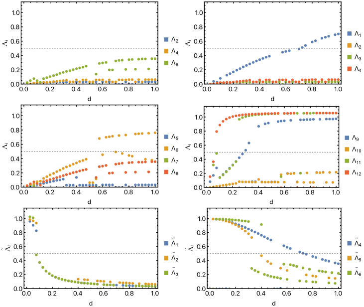
Figure S2: $\bm{0\leq\nu<1}$ ($\bm{N_{f}=8}$). The reduced order parameter eigenvalues, $\Lambda_{i}=\lambda_{i}/\mathtt{S}$, evaluated at the stable fixed rays at each value of $d$, and with only the maximum $\Lambda_{i}$ at each $d$ presented. For this reason the curves are discontinuous. Top left panel focuses on the three distinct T-IVC orders.

Figure S3: $\bm{1\leq\nu<2}$ ($\bm{N_{f}=6}$). The reduced order parameter eigenvalues, $\Lambda_{i}=\lambda_{i}/\mathtt{S}$, evaluated at the stable fixed rays at each value of $d$, and with only the maximum $\Lambda_{i}$ at each $d$ presented.

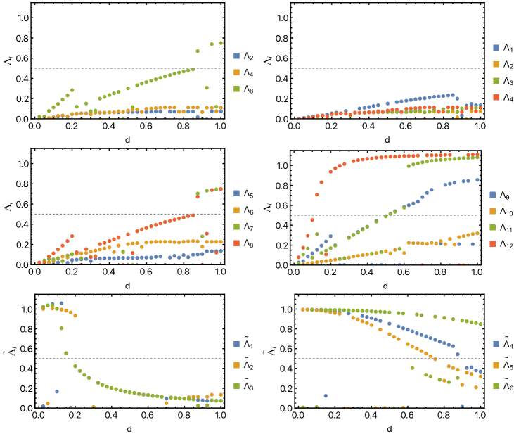
Figure S4: $\bm{2\leq\nu<3}$ ($\bm{N_{f}=4}$). The reduced order parameter eigenvalues, $\Lambda_{i}=\lambda_{i}/\mathtt{S}$, evaluated at the stable fixed rays at each value of $d$, and with only the maximum $\Lambda_{i}$ at each $d$ presented.

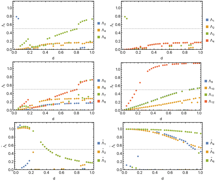
Figure S5: $\bm{3\leq\nu<4}$ ($\bm{N_{f}=2}$). The reduced order parameter eigenvalues, $\Lambda_{i}=\lambda_{i}/\mathtt{S}$, evaluated at the stable fixed rays at each value of $d$, and with only the maximum $\Lambda_{i}$ at each $d$ presented.

…

…

…

…

S5 Wess-Zumino-Witten terms

For completeness and to be self-contained, we here detail the criteria for determining the possible WZW terms discussed in the main text. We focus on the scenario with a single superconducting order parameter (two real degrees of freedom), described by the matrix $\Delta=-\Delta^{T}$ in the vicinity of the Dirac cones, and three particle-hole order parameters $m_{j}=m_{j}^{\dagger}$, $j=1,2,3$, coupling to the electrons as

$$\mathcal{H}_{C}=\sum_{\bm{k}}\left[\psi^{\dagger}_{\bm{k}}\Delta\psi^{\dagger}_{-\bm{k}}+\text{h.c.}\right]+\sum_{\bm{k},j}\psi^{\dagger}_{\bm{k}}m_{j}\psi^{\phantom{\dagger}}_{\bm{k}}.$$ (S160)

At $\nu=0$, the operators $\psi^{\dagger}_{\bm{k}}$ are the same as those in Eq. (2) of the main text, i.e., 16-component spinors in sublattice, mini-valley, valley, and spin space, and, hence, $\Delta$ and $m_{j}$ are $16\times 16$ matrices. Due to the Dirac revival, these are only 8-component field operators and, thus, $8\times 8$ order parameters at $\nu=2$. Focusing on spin-valley locking, these remaining eight flavor degrees of freedom arise from sublattice, mini-valley, and the combined spin-valley index (with Pauli matrices $\gamma_{j}$).

As shown in Ref. Christos2020 , a WZW term arises if all of the following properties hold

$$\Gamma_{i}\Delta =-\Delta\Gamma_{i}^{T}\neq 0,\quad\quad i=1,2,$$ (S161a)

$$m_{j}\Delta =\Delta m_{j}^{T}\neq 0,\quad\quad\,\,j=1,2,3,$$ (S161b)

$$\text{tr}\left[\Gamma_{i_{1}}\Gamma_{i_{2}}m_{j_{1}}m_{j_{2}}m_{j_{3}}\right] =k\,\epsilon_{i_{1},i_{2},j_{1},j_{2},j_{3}},\quad k\neq 0.$$ (S161c)

Here, $\Gamma_{i=1,2}$ are the two Dirac matrices parametrising the non-interacting Hamiltonian, i.e., $\Gamma_{1}=\tau_{z}\alpha_{x}=\tau_{z}\sigma_{x}$, $\Gamma_{2}=\tau_{z}\alpha_{y}=\sigma_{y}$ for $\nu=0$ [as directly follows from Eq. (1)] and $\Gamma_{1}=\gamma_{z}\sigma_{x}$, $\Gamma_{2}=\sigma_{y}$ for spin-valley locking at $\nu=2$.

By systematically checking which combinations $\{\Delta,m_{1,2,3}\}$ of the order parameters in Table 1 and 3 satisfy Eq. (S161), associated with a fixed ray in Table 2 at the respective filling, we find all possible WZW scenarios.

References

• (1) Y. Cao et al., “Unconventional superconductivity in magic-angle graphene superlattices”, Nature 556, 43–50 (2018).
• (2) Y. Cao et al., “Correlated insulator behaviour at half-filling in magic-angle graphene superlattices”, Nature 556, 80–84 (2018).
• (3) M. Yankowitz et al., “Tuning superconductivity in twisted bilayer graphene”, Science 363, 6431 (2019).
• (4) X. Lu et al., “Superconductors, orbital magnets and correlated states in magic-angle bilayer graphene”, Nature 574, 653–657 (2019).
• (5) Y. Cao et al., “Strange Metal in Magic-Angle Graphene with near Planckian Dissipation”, Phys. Rev. Lett. 124, 076801 (2020).
• (6) H. Polshyn et al., “Large linear-in-temperature resistivity in twisted bilayer graphene”, Nat. Phys. 15, 1011–1016 (2019).
• (7) Y. Xie et al., “Spectroscopic signatures of many-body correlations in magic-angle twisted bilayer graphene”, Nature 572, 101–105 (2019).
• (8) S. L. Tomarken et al., “Electronic Compressibility of Magic-Angle Graphene Superlattices”, Phys. Rev. Lett. 123, 046601 (2019).
• (9) Y. Jiang et al., “Charge order and broken rotational symmetry in magic-angle twisted bilayer graphene”, Nature 573, 91–95 (2019).
• (10) Y. Choi et al., “Electronic correlations in twisted bilayer graphene near the magic angle”, Nat. Phys. 15, 1174–1180 (2019).
• (11) A. Kerelsky et al., “Maximized electron interactions at the magic angle in twisted bilayer graphene”, Nature 572, 95 (2019).
• (12) Y. Saito et al., “Hofstadter subband ferromagnetism and symmetry-broken Chern insulators in twisted bilayer graphene” Nat. Phys. 17, 478–481 (2021).
• (13) I. Das et al., “Observation of Reentrant Correlated Insulators and Interaction-Driven Fermi-Surface Reconstructions at One Magnetic Flux Quantum per Moiré Unit Cell in Magic-Angle Twisted Bilayer Graphene”, Phys. Rev. Lett. 128, 217701 (2022).
• (14) Y. Cao et al., “Nematicity and competing orders in superconducting magic-angle graphene”, Science 372, 6539 (2021).
• (15) A. K. Paul et al., “Interaction-driven giant thermopower in magic-angle twisted bilayer graphene”, Nat. Phys. 18, 691–698 (2022).
• (16) D. Wong et al., “Cascade of electronic transitions in magic-angle twisted bilayer graphene”, Nature 582, 198–202 (2020).
• (17) E. Morissette et al., “Dirac revivals drive a resonance response in twisted bilayer graphene”, Nat. Phys. (2023).
• (18) M. Oh et al., “Evidence for unconventional superconductivity in twisted bilayer graphene”, Nature 600, 240–245 (2021).
• (19) H. Kim et al., “Evidence for unconventional superconductivity in twisted trilayer graphene”, Nature 606, 494–500 (2022).
• (20) J. M. Park et al., “Tunable strongly coupled superconductivity in magic-angle twisted trilayer graphene”, Nature 590, 249–255 (2021).
• (21) K. P. Nuckolls et al., “Quantum textures of the many-body wavefunctions in magic-angle graphene”, arXiv:2303.00024 [cond-mat.mes-hall].
• (22) H. Kim et al., “Imaging inter-valley coherent order in magic-angle twisted trilayer graphene”, arXiv:2304.10586 [cond-mat.str-el].
• (23) A. T. Pierce et al., “Unconventional sequence of correlated Chern insulators in magic-angle twisted bilayer graphene”, Nat. Phys. 17, 1210–1215 (2021).
• (24) P. Stepanov et al., “Competing Zero-Field Chern Insulators in Superconducting Twisted Bilayer Graphene”, Phys. Rev. Lett. 127, 197701 (2021).
• (25) S. Bhowmik et al., “Broken-symmetry states at half-integer band fillings in twisted bilayer graphene”, Nat. Phys. 18, 639–643 (2022).
• (26) Y. Choi et al., “Correlation-driven topological phases in magic-angle twisted bilayer graphene” Nature 589, 536–541 (2021).
• (27) K. P. Nuckolls et al., “Strongly correlated Chern insulators in magic-angle twisted bilayer graphene”, Nature 588, 610–615 (2020).
• (28) J. M. Park et al., “Flavour Hund’s coupling, Chern gaps and charge diffusivity in moiré graphene”, Nature 592, 43–48 (2021).
• (29) Y. Xu et al., “Correlated insulating states at fractional fillings of moiré superlattices”, Nature 587, 214–218 (2020).
• (30) Y. Xie et al., “Fractional Chern insulators in magic-angle twisted bilayer graphene”, Nature 600, 439–443 (2021).
• (31) I. Das et al., “Symmetry-broken Chern insulators and Rashba-like Landau-level crossings in magic-angle bilayer graphene”, Nat. Phys. 17, 710–714 (2021).
• (32) M. Serlin et al., Intrinsic quantized anomalous hall effect in a moiré heterostructure, Science 367, 900–903 (2019).
• (33) R. Polski et al., “Hierarchy of Symmetry Breaking Correlated Phases in Twisted Bilayer Graphene”, arXiv:2205.05225 [cond-mat.str-el].
• (34) Y. Saito et al., “Isospin Pomeranchuk effect in twisted bilayer graphene”, Nature 592, 220–224 (2021).
• (35) A. L. Sharpe et al., “Emergent ferromagnetism near three-quarters filling in twisted bilayer graphene”, Science 365, 6453 (2019).
• (36) J. Liu and X. Dai, “Orbital magnetic states in moiré graphene systems”, Nat. Rev. Phys. 3, 367–382 (2021).
• (37) A. L. Sharpe et al., “Evidence of Orbital Ferromagnetism in Twisted Bilayer Graphene Aligned to Hexagonal Boron Nitride”, Nano Lett. 21, 10, 4299–4304 (2021).
• (38) J.X. Lin et al., “Spin-orbit–driven ferromagnetism at half moiré filling in magic-angle twisted bilayer graphene”, Science 375, 6579 (2022).
• (39) S. Grover et al., “Chern mosaic and Berry-curvature magnetism in magic-angle graphene”, Nat. Phys. 18, 885–892 (2022).
• (40) A. Uri et al., “Mapping the twist-angle disorder and Landau levels in magic-angle graphene”, Nature 581, 47–52 (2020).
• (41) C. L. Tschirhart et al., “Imaging orbital ferromagnetism in a moiré Chern insulator”, Science 372, 6548 (2021).
• (42) Y. Kim et al., “Odd integer quantum hall states with interlayer coherence in twisted bilayer graphene”, Nano Lett. 21, 4249–4254 (2021).
• (43) H.-C. Po, L. Zou, A. Vishwanath, and T. Senthil, “Origin of Mott Insulating Behavior and Superconductivity in Twisted Bilayer Graphene”, Phys. Rev. X 8, 031089 (2018).
• (44) H.-C. Po, L. Zou, T. Senthil, and A. Vishwanath, “Faithful tight-binding models and fragile topology of magic-angle bilayer graphene”, Phys. Rev. B 99, 195455 (2019).
• (45) C. Xu and L. Balents, “Topological Superconductivity in Twisted Multilayer Graphene”, Phys. Rev. Lett. 121, 087001 (2018).
• (46) G. Tarnopolsky, A. J. Kruchkov, and A. Vishwanath, “Origin of Magic Angles in Twisted Bilayer Graphene”, Phys. Rev. Lett. 122, 106405 (2019).
• (47) B. A. Bernevig, Z.-D. Song, N. Regnault, and B. Lian, “Twisted bilayer graphene. I. Matrix elements, approximations, perturbation theory, and a $k\cdot p$ two-band model”, Phys. Rev. B 103, 205411 (2021).
• (48) Z.-D. Song, B. Lian, N. Regnault, and B. A. Bernevig, “Twisted bilayer graphene. II. Stable symmetry anomaly”, Phys. Rev. B 103, 205412 (2021).
• (49) B. A. Bernevig, Z.-D. Song, N. Regnault, and B. Lian, “Twisted bilayer graphene. III. Interacting Hamiltonian and exact symmetries”, Phys. Rev. B 103, 205413 (2021).
• (50) F. Xie et al., “Twisted bilayer graphene. VI. An exact diagonalization study at nonzero integer filling”, Phys. Rev. B 103, 205416 (2021).
• (51) Z. Song et al., “All Magic Angles in Twisted Bilayer Graphene are Topological”, Phys. Rev. Lett. 123, 036401 (2019).
• (52) Z.-D. Song, and B. A. Bernevig, “Magic-Angle Twisted Bilayer Graphene as a Topological Heavy Fermion Problem”, Phys. Rev. Lett. 129, 047601 (2022).
• (53) H. Isobe, N. F. Q. Yuan, and L. Fu, “Unconventional Superconductivity and Density Waves in Twisted Bilayer Graphene”, Phys. Rev. X 8, 041041 (2018).
• (54) Y.-Z. You and A. Vishwanath, “Superconductivity from valley fluctuations and approximate SO(4) symmetry in a weak coupling theory of twisted bilayer graphene”, npj Quantum Mater. 4, 16 (2019).
• (55) C.-C. Liu, L.-D. Zhang, W.-Q. Chen, and F. Yang, “Chiral Spin Density Wave and $d+id$ Superconductivity in the Magic-Angle-Twisted Bilayer Graphene”, Phys. Rev. Lett. 121, 217001 (2018).
• (56) J. González and T. Stauber, “Kohn-Luttinger Superconductivity in Twisted Bilayer Graphene”, Phys. Rev. Lett. 122, 026801 (2019).
• (57) L. Classen, C. Honerkamp, and M. M. Scherer, “Competing phases of interacting electrons on triangular lattices in moiré heterostructures”, Phys. Rev. B 99, 195120 (2019).
• (58) Y.-P. Lin and R. Nandkishore, “A chiral twist on the high-$T_{c}$ phase diagram in Moiré heterostructures”, Phys. Rev. B 100, 085136 (2019).
• (59) D. V. Chichinadze, L. Classen, and A. V. Chubukov, “Valley magnetism, nematicity, and density wave orders in twisted bilayer graphene”, Phys. Rev. B 102, 125120 (2020).
• (60) D. V. Chichinadze, L. Classen, and A. V. Chubukov, “Nematic superconductivity in twisted bilayer graphene”, Phys. Rev. B 101, 224513 (2020).
• (61) F. Guinea and N. R. Walet, “Electrostatic effects, band distortions, and superconductivity in twisted graphene bilayers”, Proc. Natl. Acad. Sci. U.S.A. 115, 13174 (2018).
• (62) B. A. Bernevig et al., “Twisted bilayer graphene. V. Exact analytic many-body excitations in Coulomb Hamiltonians: Charge gap, Goldstone modes, and absence of Cooper pairing”, Phys. Rev. B 103, 205415 (2021).
• (63) Y. H. Kwan et al., Kekulé Spiral Order at All Nonzero Integer Fillings in Twisted Bilayer Graphene Phys. Rev. X 11, 041063 (2021).
• (64) S. Liu, E. Khalaf, J.-Y. Lee, and A. Vishwanath, “Nematic topological semimetal and insulator in magic-angle bilayer graphene at charge neutrality”, Phys. Rev. Research 3, 013033 (2021).
• (65) J. Liu and X. Dai, “Theories for the correlated insulating states and quantum anomalous Hall effect phenomena in twisted bilayer graphene” Phys. Rev. B 103, 035427 (2021).
• (66) Y. H. Kwan et al., “Electron-phonon coupling and competing Kekulé orders in twisted bilayer graphene”, arXiv:2303.13602 [cond-mat.str-el]
• (67) G. Wagner et al., “Global Phase Diagram of the Normal State of Twisted Bilayer Graphene”, Phys. Rev. Lett. 128, 156401 (2022).
• (68) N. Bultinck et al.,“Ground State and Hidden Symmetry of Magic-Angle Graphene at Even Integer Filling”, Phys. Rev. X 10, 031034 (2020).
• (69) B. Lian et al., “Twisted bilayer graphene. IV. Exact insulator ground states and phase diagram”, Phys. Rev. B 103, 205414 (2021).
• (70) M. Christos, S. Sachdev, and M. S. Scheurer, “Correlated Insulators, Semimetals, and Superconductivity in Twisted Trilayer Graphene”, Phys. Rev. X 12, 021018 (2022).
• (71) Patrick J. Ledwith et al., “TB or not TB? Contrasting properties of twisted bilayer graphene and the alternating twist $n$-layer structures ($n=3,4,5,…$)”, arXiv:2111.11060 [cond-mat.str-el].
• (72) J. Kang and O. Vafek, “Strong Coupling Phases of Partially Filled Twisted Bilayer Graphene Narrow Bands”, Phys. Rev. Lett. 122, 246401 (2019).
• (73) Fang Xie et al., “Twisted symmetric trilayer graphene. II. Projected Hartree-Fock study”, Phys. Rev. B 104, 115167 (2021).
• (74) M. S. Schuerer and R. Samajdar, “Pairing in graphene-based moiré superlattices”, Phys. Rev. Research 2, 033062 (2020).
• (75) J. Yu, M. Xie, F. Wu and S. Das Sarma, “Euler-obstructed nematic nodal superconductivity in twisted bilayer graphene”, Phys. Rev. B 107, L201106 (2023).
• (76) T. J. Peltonen, R. Ojajärvi, and T. T. Heikkilä, “Mean-field theory for superconductivity in twisted bilayer graphene”, Phys. Rev. B 98, 220504(R) (2018).
• (77) X. Y. Xu, K. T. Law, and P. A. Lee, “Kekulé valence bond order in an extended Hubbard model on the honeycomb lattice with possible applications to twisted bilayer graphene”, Phys. Rev. B 98, 121406(R) (2018).
• (78) B. Lian, Z. Wang, and B. A. Bernevig, “Twisted Bilayer Graphene: A Phonon Driven Superconductor”, Phys. Rev. Lett. 122, 257002 (2019).
• (79) F. Wu, A. H. MacDonald, and I. Martin, “Theory of Phonon-Mediated Superconductivity in Twisted Bilayer Graphene”, Phys. Rev. Lett. 121, 257001 (2018).
• (80) Y.-H. Zhang, D. Mao, Y. Cao, P. Jarillo-Herrero, and T. Senthil, “Nearly flat Chern bands in moiré superlattices”, Physical Review B 99, 075127 (2019).
• (81) N. F. Q. Yuan and L. Fu, “Model for the metal-insulator transition in graphene superlattices and beyond”, Phys. Rev. B 98, 045103 (2018).
• (82) J. Ahn, S. Park, and B.-J. Yang, “Failure of Nielsen-Ninomiya Theorem and Fragile Topology in Two-Dimensional Systems with Space-Time Inversion Symmetry: Application to Twisted Bilayer Graphene at Magic Angle”, Phys. Rev. X 9, 021013 (2019).
• (83) A. Julku et al., “Superfluid weight and Berezinskii-Kosterlitz-Thouless transition temperature of twisted bilayer graphene”, Phys. Rev. B 101, 060505 (2020).
• (84) B. Padhi, A. Tiwari, T. Neupert, and S. Ryu, “Transport across twist angle domains in moiré graphene”, Phys. Rev. Research 2, 033458 (2020).
• (85) R. M. Fernandes and L. Fu, “Charge-$4e$ superconductivity from multicomponent nematic pairing: Application to twisted bilayer graphene”, Phys. Rev. Lett. 127 047001 (2021).
• (86) Y. H. Kwan et al., “Domain wall competition in the Chern insulating regime of twisted bilayer graphene”, Phys. Rev. B 104, 115404 (2021).
• (87) B. Padhi, C. Setty, and P. W. Phillips, “Doped Twisted Bilayer Graphene near Magic Angles: Proximity to Wigner Crystallization, Not Mott Insulation”, Nano Lett. 18, 10, 6175–6180 (2018).
• (88) A. Thomson and J. Alicea, “Recovery of massless Dirac fermions at charge neutrality in strongly interacting twisted bilayer graphene with disorder”, Phys. Rev. B 103, 125138 (2021).
• (89) T. Yu, D. M. Kennes, A. Rubio, and M. A. Sentef, “Nematicity Arising from a Chiral Superconducting Ground State in Magic-Angle Twisted Bilayer Graphene under In-Plane Magnetic Fields” Phys. Rev. Lett. 127, 127001 (2021).
• (90) E. Khalaf, P. Ledwith, and A. Vishwanath, “Symmetry constraints on superconductivity in twisted bilayer graphene: Fractional vortices, $4e$ condensates, or nonunitary pairing”, Phys. Rev. B 105, 224508 (2022).
• (91) E. Lake, A. S. Patri, and T. Senthil, “Pairing symmetry of twisted bilayer graphene: A phenomenological synthesis” Phys. Rev. B 106, 104506 (2022).
• (92) Y.-H. Zhang, H. C. Po, and T. Senthil, “Landau level degeneracy in twisted bilayer graphene: Role of symmetry breaking”, Phys. Rev. B 100, 125104 (2019).
• (93) J.-Y. Lee et al., “Theory of correlated insulating behaviour and spin-triplet superconductivity in twisted double bilayer graphene”, Nat. Commun. 10, 5333 (2019).
• (94) M. Christos, S. Sachdev, and M. S. Scheurer, “Nodal band-off-diagonal superconductivity in twisted graphene superlattices” arXiv:2303.17529 [cond-mat.supr-con].
• (95) B. Roy and V. Juričić, “Unconventional superconductivity in nearly flat bands in twisted bilayer graphene”, Phys. Rev. B 99, 121407(R) (2019).
• (96) S.K. Firoz Islam, A. Yu. Zyuzin, A. A. Zyuzin, “Unconventional superconductivity with preformed pairs in twisted bilayer graphene”, Phys. Rev. B 107, L060503 (2023).
• (97) E. Brillaux, D. Carpentier, A. A. Fedorenko, and L. Savary, “Analytical renormalization group approach to competing orders at charge neutrality in twisted bilayer graphene”, Phys. Rev. Research 4, 033168 (2022).
• (98) N. Parthenios and L. Classen, “Twisted bilayer graphene at charge neutrality: competing orders of SU(4) Dirac fermions”, arXiv:2305.06949 [cond-mat.str-el].
• (99) J. M. B. Lopes dos Santos, N. M. R. Peres, and A. H. Castro Neto, “Continuum model of the twisted graphene bilayer”, Phys. Rev. B 86, 155449 (2012).
• (100) R. Bistritzer and A. H. MacDonald, “Moiré bands in twisted double-layer graphene”, Proc. Natl. Acad. Sci. U.S.A. 108 (30) 12233-12237 (2011).
• (101) M. Koshino et al., Maximally Localized Wannier Orbitals and the Extended Hubbard Model for Twisted Bilayer Graphene Phys. Rev. X 8, 031087 (2018).
• (102) H.-C. Po, L. Zou, A. Vishwanath, and T. Senthil, “Band structure of twisted bilayer graphene: Emergent symmetries, commensurate approximants, and Wannier obstructions” Phys. Rev. B 98, 085435 (2018).
• (103) E. Khalaf, A. J. Kruchkov, G. Tarnopolsky, and A. Vishwanath, “Magic angle hierarchy in twisted graphene multilayers”, Phys. Rev. B 100, 085109 (2019).
• (104) H. Yoo et al., “Atomic and electronic reconstruction at the van der Waals interface in twisted bilayer graphene”, Nat. Mater. 18, 448-453 (2019).
• (105) G. A. Tritsaris et al., “Electronic structure calculations of twisted multi-layer graphene superlattices”, 2D Mater. 7, 035028 (2020).
• (106) S. Carr, S. Fang, Z. Zhu, and E. Kaxiras, “Exact continuum model for low-energy electronic states of twisted bilayer graphene”, Phys. Rev. Research 1, 013001 (2019).
• (107) S. Carr et al., “Derivation of Wannier orbitals and minimal-basis tight-binding Hamiltonians for twisted bilayer graphene: First-principles approach”, Phys. Rev. Research 1, 033072 (2019).
• (108) Jian Kang and Oskar Vafek “Symmetry, Maximally Localized Wannier States, and a Low-Energy Model for Twisted Bilayer Graphene Narrow Bands” Phys. Rev. X 8, 031088 (2018).
• (109) J. Zang et al., “Real space representation of topological system: twisted bilayer graphene as an example”, arXiv:2210.11573 [cond-mat.mes-hall].
• (110) U. Zondinger et al., “Cascade of phase transitions and Dirac revivals in magic-angle graphene”, Nature 582, 203–208 (2020).
• (111) X. Liu et al., “Tuning electron correlation in magic-angle twisted bilayer graphene using Coulomb screening”, Science 371, 6535 (2021).
• (112) P. Stepanov et al., “Untying the insulating and superconducting orders in magic-angle graphene”, Nature 583, 1 (2020).
• (113) Y. Saito et al., “Independent superconductors and correlated insulators in twisted bilayer graphene” Nat. Phys. 16, 926–930 (2020).
• (114) J. M. Park et al., “Tunable Phase Boundaries and Ultra-Strong Coupling Superconductivity in Mirror Symmetric Magic-Angle Trilayer Graphene”, Nature 590, 249–255 (2021).
• (115) Z. Hao et al.,“Electric field–tunable superconductivity in alternating-twist magic-angle trilayer graphene”, Science 371, 6534 (2021).
• (116) Y. Cao et al., “Pauli-limit violation and re-entrant superconductivity in moiré graphene”, Nature 595, 526–531 (2021).
• (117) P. Siriviboon et al., “A new flavor of correlation and superconductivity in small twist-angle trilayer graphene”, arXiv:2112.07127 [cond-mat.mes-hall].
• (118) Y. Zhang et al., “Ascendance of Superconductivity in Magic-Angle Graphene Multilayers”, arXiv:2112.09270 [cond-mat.supr-con].
• (119) Y. Sheffer, R. Queiroz, and A. Stern, “Symmetries as the Guiding Principle for Flattening Bands of Dirac Fermions”, Phys. Rev. X 13, 021012 (2023).
• (120) T. Li, M. Geier, J. Ingham, and H. D. Scammell, “Higher-order topological superconductivity from repulsive interactions in kagome and honeycomb systems”, 2D Mater. 9, 015031 (2022).
• (121) H. D. Scammell, J. Ingham, M. Geier, and T. Li, “Intrinsic first and higher-order topological superconductivity in a doped topological insulator”, Phys. Rev. B 105, 195149 (2022).
• (122) T. Li, J. Ingham and H. D. Scammell “Artificial graphene: Unconventional superconductivity in a honeycomb superlattice”, Phys. Rev. Research 2, 043155 (2020).
• (123) O. Vafek and K. Yang, “Many-body instability of Coulomb interacting bilayer graphene: Renormalization group approach”, Phys. Rev. B 81, 041401(R) (2010).
• (124) K. Sun, H. Yao, E. Fradkin, and S. A. Kivelson, “Topological Insulators and Nematic Phases from Spontaneous Symmetry Breaking in 2D Fermi Systems with a Quadratic Band Crossing”, Phys. Rev. Lett. 103, 046811 (2009).
• (125) J. Wang, C. Ortix, J. van den Brink, and D. V. Efremov, “Fate of interaction-driven topological insulators under disorder” Phys. Rev. B 96, 201104(R) (2017).
• (126) S. Uebelacker and C. Honerkamp, “Instabilities of quadratic band crossing points”, Phys. Rev. B 84, 205122 (2011).
• (127) P A. Volkov, J. H. Wilson, Kevin P. Lucht, and J. H. Pixley, “Magic angles and correlations in twisted nodal superconductors”, Phys. Rev. B 107, 174506 (2023).
• (128) T. Giamarchi, Quantum Physics in One Dimension, Oxford University Press, Oxford, 2004.
• (129) C. Platt, W. Hanke, and R. Thomale, Functional Renormalization Group for Multi-Orbital Fermi Surface Instabilities, Adv. Phys. 62, 453 (2013).
• (130) W. Metzner et al., “Functional renormalization group approach to correlated fermion systems”, Rev. Mod. Phys. 84, 299 (2012).
• (131) M. Salmhofer and C. Honerkamp, “Fermionic Renormalization Group Flows: Technique and Theory”, Prog. Theor. Phys. 105, 1 (2001).
• (132) J. Polchinski, “Renormalization and effective lagrangians”, Nucl. Phys. B 231, 269-295 (1984).
• (133) C. Wetterich, “Exact evolution equation for the effective potential”, Phys. Lett. B 301 90-94 (1993).
• (134) D. M. Kennes, J. Lischner, and C. Karrasch, “Strong correlations and $d+id$ superconductivity in twisted bilayer graphene”, Phys. Rev. B 98, 241407(R) (2019).
• (135) L. Klebl, D. M. Kennes, and C. Honerkamp, “Functional renormalization group for a large moiré unit cell” Phys. Rev. B 102, 085109 (2020).
• (136) S. Maiti and A. V. Chubukov, “Superconductivity from repulsive interaction”, AIP Conference Proceedings 1550, 3 (2013).
• (137) L. Classen et al., “Competing orders at higher-order Van Hove points”, Phys. Rev. B 102, 125141 (2020).
• (138) H. J. Schulz, “Superconductivity and Antiferromagnetism in the Two-Dimensional Hubbard Model: Scaling Theory”, Europhys. Lett. 4, 609-615 (1987).
• (139) N. Furukawa, T. M. Rice and M. Salmhofer, “Truncation of a Two-Dimensional Fermi Surface due to Quasiparticle Gap formation at the Saddle Points”, Phys. Rev. Lett. 81, 3195-3198 (1998).
• (140) R. Nandkishore, L. S. Levitov and A. V. Chubukov, “Chiral superconductivity from repulsive interactions in doped graphene”, Nat. Phys. 8, 158-163 (2012).
• (141) Y.-M. Wu, R. Thomale, and S. Raghu, “Sublattice Interference promotes Pair Density Wave order in Kagome Metals”, arXiv:2211.01388v1 [cond-mat.str-el].
• (142) T. Li, J. Ingham, and H. D. Scammell, “Nested Fermi surfaces and correlated electronic phases in hole-doped semiconductor quantum wells”, Phys. Rev. B 105, 115302 (2022).
• (143) H. D. Scammell, J. Ingham, T. Li, and O. P. Sushkov, “Chiral excitonic order from twofold van Hove singularities in kagome metals”, Nat. Commun. 14, 605 (2023).
• (144) R. Samajdar et al., “Electric-field-tunable electronic nematic order in twisted double-bilayer graphene”, 2D Mater. 8, 034005 (2021).
• (145) J. A. Sobral et al., “Machine Learning Microscopic Form of Nematic Order in twisted double-bilayer graphene”, arXiv:2302.12274 [cond-mat.str-el].
• (146) H. Sainz-Cruz et al., “Junctions and Superconducting Symmetry in Twisted Bilayer Graphene”, Phys. Rev. Lett. 131, 016003 (2023).
• (147) P. P. Poduval and M. S. Scheurer, “Vestigial singlet pairing in a fluctuating magnetic triplet superconductor: Applications to graphene moiré systems”, arXiv:2301.01344 [cond-mat.supr-con].
• (148) D. Călugăru et al., “Spectroscopy of Twisted Bilayer Graphene Correlated Insulators” Phys. Rev. Lett. 129, 117602 (2022).
• (149) J. P. Hong, T. Soejima and M. P. Zalatel, “Detecting symmetry breaking in magic angle graphene using scanning tunnelling microscopy”, Phys. Rev. Lett. 129, 147001 (2022).
• (150) T. Grover and T. Senthil, “Topological Spin Hall States, Charged Skyrmions, and Superconductivity in Two Dimensions”, Phys. Rev. Lett. 100, 156804 (2008).
• (151) S. Chatterjee, N. Bultinck, and M. P. Zaletel, “Symmetry breaking and skyrmionic transport in twisted bilayer graphene”, Phys. Rev. B 101, 165141 (2020).
• (152) E. Khalaf et al., “Charged Skyrmions and Topological Origin of Superconductivity in Magic Angle Graphene”, Sci. Adv. 7 19 (2021).
• (153) M. Christos, S. Sachdev, and M. S. Scheurer, “Superconductivity, correlated insulators, and Wess–Zumino–Witten terms in twisted bilayer graphene”, Proc. Natl. Acad. Sci. U.S.A. 117, 29543–29554 (2020).
• (154) S. Chatterjee, M. Ippoliti, and M. P. Zaletel, “Skyrmion superconductivity: DMRG evidence for a topological route to superconductivity”, Phys. Rev. B 106, 035421 (2022).
• (155) Y. H. Kwan et al., “Skyrmions in twisted bilayer graphene: stability, pairing, and crystallization”, Phys. Rev. X 12, 031020 (2022).
• (156) Y. Zhang et al., “Enhanced superconductivity in spin–orbit proximitized bilayer graphene”, Nature 613, 268–273 (2023).
• (157) S. Illani, private communication.
• (158) This interpretation is supported by the dependence of the compressibility $d\mu/dn\sim n^{-1/2}$ on the excess density relative to integer fillings $n$, indicating a Dirac dispersion in the immediate vicinity of these densities Zondinger2020 , and is also consistent with a range of other phenomena observed in TBG, e.g. the reset of the density seen in quantum oscillations, the doping dependence of the thermopower response Paul2022 , the results of electron spin resonance Morissette2023 , and the density of states seen in STM Wong2020 .
• (159) The passing of the Fermi level through a vHS should be accompanied by a change in the sign of the Hall density – distinct from the signatures of a Dirac revival, near which the Hall density resets to zero but does not change sign. In the vicinity of the magic angle, signatures of a vHS disappear and are replaced with the appearance of Dirac revivals for $T\lesssim 20$ K, though the angles at which this occurs differ for electron- and hole-doping. Strikingly, the angles at which vHS appear on the electron/hole doped side are precisely those angles at which $T_{c}$ drops to zero, whereas those angles at which the revivals are most robust are those angles at which $T_{c}$ is maximised. For instance in Ref. Polski2022 , near $\theta=0.88^{\circ}$ a vHS appears on the hole-doped side, where $T_{c}$ vanishes, while a reset appears near $\nu=+2$ where $T_{c}=0.8$ K is maximal. By contrast, near $\theta=1.1^{\circ}$, a vHS appears on the electron-doped side where superconductivity is suppressed, whereas a reset appears near $\nu=-2$ where $T_{c}=1.5$ K is maximal. Hence, experimental evidence indicates that superconductivity is in fact consistently suppressed when the chemical potential lies in the vicinity of a vHS, and strongest when signatures of Dirac revivals are observed. Furthermore, in twisted trilayer graphene, where Dirac revivals also appear, the application of a displacement field can eliminate the Dirac revival and lead to the emergence of vHS seen in the doping dependence of the Hall density. In this situation, the same trend is observed: superconductivity appears near revivals but is suppressed near vHS, see Park2021a ; Hao2021 ; Cao2021a . This has been seen as a puzzle – since a large density of states is typically favourable for superconductivity – but is quite natural in our analysis, which argues that the interaction physics of the quadratic Dirac theory is essential for the appearance of superconductivity.
• (160) In the Bistritzer-MacDonald model, this particle-hole symmetry ${\cal P}\mathcal{H}_{\text{BM}}(\bm{k}){\cal P}^{-1}=-\mathcal{H}_{\text{BM}}(-\bm{k})$ becomes exact upon neglecting the twist angle dependence of the monolayer Hamiltonian (see the Supplementary Material).
• (161) In the Bistritzer-MacDonald continuum model, this requires setting $w_{0}=0$. Here we do not require $w_{0}=0$, and so ${\cal C}$ is an approximate low-energy symmetry of the Dirac theory, rather than an exact symmetry of the full theory away from the Dirac points.
• (162) In the presence of lattice relaxation, there is no angle where the velocity exactly vanishes in the full Bistritzer-MacDonald model, where $\mathcal{P}$ is only an approximate symmetry.
• (163) Thermopower experiments suggest that the Dirac-revived bands may already be particle-hole asymmetric at some integer fillings Paul2022 ; in this case, one may have $d<1$ even at the band touching point. This may also affect the relative strength of our coupling constants, and we leave the incorporation of weak particle-hole symmetry breaking to future work. We also note that our RG method can exactly incorporate $\mu$, rather than approximately via the $d$ factor, as is discussed in the Supplemental Material, but the the $d$ approximation will be useful to us in describe the RG fixed rays described in the following section.
• (164) Note that the inter-moiré-valley states break moiré translational symmetry, and so are properly classified by irreducible representations of the moiré space group. We refer to this state as $E$ to denote its irrep under $D_{3}$, as per Table 1.
• (165) C.f. the discussion in Lake2022 , which also advocates for spin-valley locking at $|\nu|=2$.
• (166) Experiments in twisted trilayer graphene found that superconductivity disappears after the Dirac revival at $\nu=\pm 3$ Park2021a . This observation is also naturally explained by our theory – we find the superconducting states that appear after the $|\nu|=3$ revival are fragile to disorder and trigonal warping, whereas the superconducting states near $|\nu|=2$ are more robust.
• (167) These ranges of twist angles were also precisely those at which superconductivity was observed for $\nu>0$ and $\nu<0$ respectively. Similarly, Ref. Zondinger2020 saw resets at all integer fillings for $\nu>0$, but only at larger twist angles for $\nu<0$ and only near $\nu=-2,-1$.