Black Holes as Neutrino Factories
Abstract
Ultralight bosons can grow substantially in the vicinity of a black hole, through superradiant energy extraction. Consequently, such bosons can potentially reach field values close to the Planck scale, making black holes powerful transducers of such fields. If a scalar field couples to neutrino, it can trigger parametric production of neutrinos, and potentially quench their superradiant growth. During this saturation phase, scalar clouds can accelerate neutrinos to the TeV energy scale, generating fluxes that surpass those produced by atmospheric neutrinos.
I Introduction.
Hypothetical bosons with ultralight masses are promising candidates for beyond-the-standard-model particle physics. They are motivated by their potential to explain the smallness of the neutron electric dipole moment Peccei and Quinn (1977), and they are natural outcomes of fundamental theories with extra dimensions Svrcek and Witten (2006); Abel et al. (2008); Arvanitaki et al. (2010); Goodsell et al. (2009). When these bosons comprise dark matter Preskill et al. (1983); Abbott and Sikivie (1983); Dine and Fischler (1983); Nelson and Scholtz (2011) and possess masses lower than eV, they behave as coherent waves due to their substantial occupation numbers Hu et al. (2000).
The signals associated with ultralight bosons are typically proportional to their energy density or field value. When the Compton wavelength of these bosons is comparable to the gravitational radius of a rapidly rotating black hole (BH), a bound state can form through the superradiance mechanism, which involves the extraction of the BH rotational energy Penrose and Floyd (1971); Zel’Dovich (1971); Brito et al. (2015a). The process then leads to the condensation of a bosonic structure – a boson cloud – in the BH exterior Detweiler (1980); Cardoso and Yoshida (2005); Dolan (2007). Superradiant clouds can reach a total mass of approximately of the BH mass Brito et al. (2015b); East and Pretorius (2017); Herdeiro et al. (2022), corresponding to a field value approaching the Planck scale Chen et al. (2023a). Thus, Kerr BHs can serve as powerful transducers for ultralight bosons Brito et al. (2015a). Detection based on superradiance does not necessarily require ultralight bosons to constitute the majority of dark matter. It can be achieved, for example, through the spin-down of BHs Arvanitaki and Dubovsky (2011); Arvanitaki et al. (2015); Brito et al. (2015b); Baryakhtar et al. (2017); Brito et al. (2017a); Cardoso et al. (2018); Davoudiasl and Denton (2019); Brito et al. (2020); Stott (2020); Ünal et al. (2021); Saha et al. (2022), gravitational-wave signals from boson clouds Arvanitaki and Dubovsky (2011); Yoshino and Kodama (2012, 2014); Arvanitaki et al. (2015); Yoshino and Kodama (2015); Baryakhtar et al. (2017); Brito et al. (2017b, a); Isi et al. (2019); Siemonsen and East (2020); Sun et al. (2020); Palomba et al. (2019); Brito et al. (2020); Zhu et al. (2020); Tsukada et al. (2021); Yuan et al. (2021a); Abbott et al. (2022a); Yuan et al. (2022); Chen et al. (2023a); Brito and Shah (2023), and axion cloud-induced birefringence Chen et al. (2020); Yuan et al. (2021b); Chen et al. (2022a, b).
The couplings between ultralight bosons and standard model neutrinos are prevalent in various beyond-standard-model theories, which are motivated by neutrino mass generation Gelmini and Roncadelli (1981); Chikashige et al. (1981); Aulakh and Mohapatra (1982) and grand unification theories Georgi and Glashow (1974); Pati and Salam (1974); Mohapatra and Pati (1975); Fritzsch and Minkowski (1975); Georgi (1975). Nevertheless, investigating these couplings presents significant challenges due to the inherent difficulties associated with neutrino production and detection. The constraints on these couplings primarily arise from neutrino self-interactions mediated by ultralight bosons Kolb and Turner (1987); Huang et al. (2018); Brune and Päs (2019); Forastieri et al. (2019); Berryman et al. (2022); Li and Xu (2023), and distortions in neutrino oscillations caused by ultralight dark matter Reynoso and Sampayo (2016); Berlin (2016); Krnjaic et al. (2018); Brdar et al. (2018); Davoudiasl et al. (2018); Liao et al. (2018); Capozzi et al. (2018); Huang and Nath (2018); Farzan (2019); Cline (2020); Dev et al. (2021); Losada et al. (2022); Huang and Nath (2022); Chun (2021); Dev et al. (2023); Losada et al. (2023a); Brzeminski et al. (2022); Alonso-Álvarez et al. (2023); ChoeJo et al. (2023); Losada et al. (2023b).
In this work, we demonstrate that scalar clouds surrounding BHs can generate substantial neutrino emissions through parametric production Greene and Kofman (1999, 2000). Moreover, the spatial gradient of scalar clouds can efficiently accelerate the produced neutrinos to TeV-level energies. Given the significant field values achievable through superradiant production, a deeper range of coupling constants can be explored by comparing the anticipated fluxes with those observed in diffusive atmospheric neutrinos Vitagliano et al. (2020).
II Superradiant Clouds.
An ultralight boson field can form (quasi-)bound states outside a BH due to gravitational attraction. These bound states exhibit discrete quantum numbers and are influenced by the gravitational fine-structure constant, denoted as Detweiler (1980); Brito et al. (2015a). Here, is Newton’s constant, while and represent the BH mass and the boson mass, respectively. Superradiance occurs when the BH rotates at a sufficient velocity for its angular velocity to surpass the angular phase velocity of specific boson states, leading to exponential transfer of rotational energy into these states (Zel’Dovich, 1971; Brito et al., 2015a).
We focus on the superradiant ground state of a massive scalar , whose orbital angular momentum corotates with the BH. Its wave function can be approximated as Detweiler (1980)
| (1) |
in the Newtonian, limit. Here, represents the peak field value of the scalar cloud, denotes the normalized radial potential. We adopt Boyer-Lindquist coordinates , and represents the gravitational radius. It is worth noting that the total mass of the cloud, , should not exceed approximately of the BH mass. Beyond this threshold, the BH spin decreases to a value that no longer satisfies the superradiant condition, unless there is an external input of angular momentum to the BH. By considering the relationship , we observe that the field value can approach the Planck scale:
| (2) |
Hereafter, we adopt as the maximum allowable field value by setting in Eq. (2).
On the other hand, exponential growth can be halted prior to the occurrence of a strong backreaction on the BH if there exists an interaction between the boson cloud and other fields. In such cases, the cloud reaches a quasi-equilibrium state where the interaction induces a steady outflow of energy, effectively balancing the superradiant gain. Examples of such interactions include quartic self-interactions Yoshino and Kodama (2012); Fukuda and Nakayama (2020); Baryakhtar et al. (2021); Omiya et al. (2022), axion-photon coupling Rosa and Kephart (2018); Boskovic et al. (2019); Ikeda et al. (2019); Spieksma et al. (2023), and electron-positron pair production Fukuda and Nakayama (2020); Blas and Witte (2020); Siemonsen et al. (2023).
III Neutrino Emission from Scalar Clouds.
We investigate a neutrino-philic coupling between a scalar field denoted as and the left-handed neutrino , which is described using two-component spinor notation:
| (3) |
Here, represents the coupling constant. The scalar field involved in this interaction is commonly referred to as the Majoron. Its coupling has been extensively discussed in the context of mediating neutrino self-interactions, a comprehensive summary can be found in Ref. Berryman et al. (2022). Various constraints on the value of exist when considering the case of an ultralight , including supernova (SN) 1987A Kachelriess et al. (2000); Farzan (2003), double beta decay Gando et al. (2012); Brune and Päs (2019), big bang nucleosynthesis Huang et al. (2018), and the cosmic microwave background Forastieri et al. (2019); Li and Xu (2023). These studies have established an approximate upper limit of . For simplicity, we assume a universal coupling to all mass eigenstates in the following.
Given the significant field value that scalar clouds can attain and the light neutrino masses ( eV Aghanim et al. (2020); Singh and Mirza (2023)), we expect that the coupling in Eq. (3) induces a coherent oscillating mass term for neutrinos around the cloud. The amplitude of this oscillation is more significant than the bare mass of neutrino , where represents the local amplitude of the scalar field. When the effective mass, , crosses zero, neutrinos undergo parametric excitation. This production mechanism was previously studied during preheating Greene and Kofman (1999, 2000), and the average production rate per unit volume is given by
| (4) |
see Supplemental Material for details. Relativistic neutrinos are produced with an initial momentum . The corresponding de Broglie wavelength of the neutrinos, , is significantly shorter than the size of the cloud, . This allows us to safely ignore the finite-size effects when using Eq. (4).
Once produced, the neutrinos immediately experience an effective force arising from the varying mass term Uzan et al. (2020). The equation of motion for their worldline is given by:
| (5) |
Here, represents the -momentum of the neutrinos, and refers the Christoffel symbols of the Kerr metric. The spatial components of Eq. (5) contain the effective force , which accelerates the neutrinos after their production. The final accelerated energy, denoted as , can be estimated by considering the -component of Eq. (5), resulting in . It is essential to emphasize that both the spatial gradient and temporal oscillation of the cloud wave-function are necessary for the acceleration process, as demonstrated in Eq. (5). Notably, neutrinos produced during the previous crossing, having been accelerated to much higher energies than , would not influence subsequent production, akin to the pair production of millicharged particles from superconducting cavities Berlin and Hook (2020).
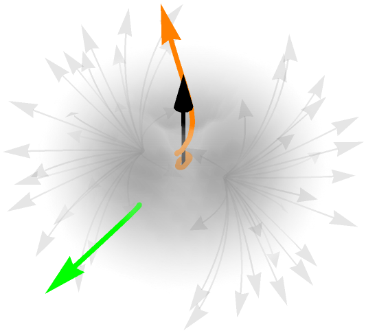

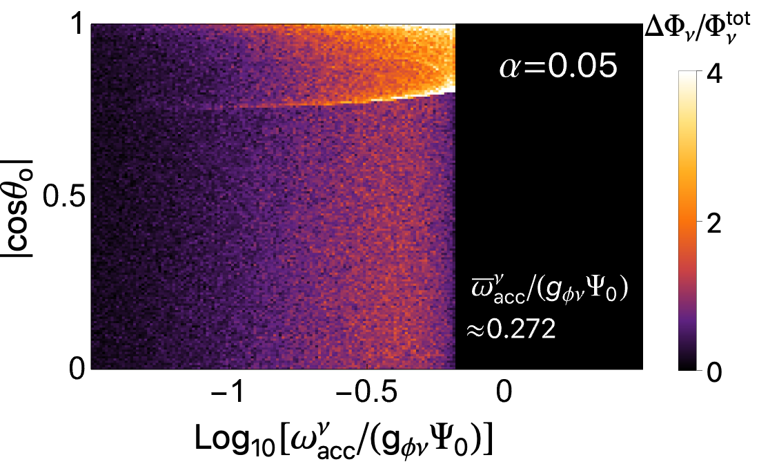
To obtain the angular distribution and spectrum of the outgoing neutrino fluxes, we perform simulations of neutrino trajectories originating from various points within scalar clouds. Details can be found in the Supplemental Material. The top panel of Fig. 1 presents two examples of neutrino trajectories emitted simultaneously from distances of (shown in orange) and (shown in green) in a scalar cloud background with . Notably, the trajectory originating from the outer region directly leaves the cloud in the radial direction, while the other trajectory first curls around the BH spin axis (shown in black). Additionally, we depict the force lines from at the production time and density of in gray. The bottom panel displays the outgoing spectrum as a function of the observer’s inclination angle . The flux is slightly higher when observed from nearly face-on angles (), forming a jet-like structure of neutrinos. This enhanced flux is primarily due to the tendency of neutrinos produced in the inner region of the cloud to be trapped in perpendicular directions while maintaining acceleration along the polar axis.
Based on our simulations, we have determined the average energy of the neutrino fluxes:
| (6) |
This value is generally independent of , as demonstrated in the Supplemental Material. We can estimate the differential fluxes received by a distant observer using
| (7) |
Here, the factor accounts for the number of neutrino mass eigenstates, and represents the distance between the BH and the observer.
We will now examine the value of in the presence of neutrino production and acceleration. This condition can be solved by ensuring that the energy carried away by neutrinos balances the energy injected by the BH through superradiance, i.e.,
| (8) |
Here, represents the scalar superradiant rate, which is approximately when Detweiler (1980). The parameter denotes the dimensionless spin parameter of the BH. Solving Eq. (8) yields the critical value for :
| (9) |
For the benchmark parameters, corresponding to a BH of mass , substituting the saturation field value from Eq. (9) into Eq. (6) and (7) yields steady emission of neutrinos with a typical energy scale of TeV and fluxes approximately equal to cm-2s-1GeV-1. Notably, these values are significantly higher than the flux of atmospheric neutrinos, which is on the order of cm-2s-1GeV-1 at TeV Vitagliano et al. (2020). Interestingly, both the neutrino fluxes and the average energy during the saturation phase increase as decreases. This behavior arises from the fact that a lower value of leads to a higher critical amplitude .
IV Spin Measurements and Neutrino Detection.
The key ingredients here are rapidly rotating BHs. Recent observations have confirmed the existence of both stellar-mass BHs and supermassive BHs, with masses ranging from a few to . Despite the lower scalar mass , which reduces the saturated neutrino fluxes and average energy, scalar clouds surrounding supermassive BHs can still generate and accelerate neutrinos, as long as Greene and Kofman (2000). Hence, we will consider both types of BHs in our analysis.
There are different methods for identifying stellar-mass BHs of interest, many of which rely on electromagnetic observations. One such method involves utilizing X-ray emissions to detect the motion of binary systems located at substantial distances Lewin et al. (1997). Spectroscopic observations, such as iron lines, can provide further information about the spins of these BHs Brenneman and Reynolds (2006). Another technique for identifying isolated BHs involves microlensing Mao et al. (2002); Bennett et al. (2002). Typically, these potential BH candidates are distributed throughout the Milky Way, with a distance of kpc from Earth. Therefore, we adopt a benchmark value of kpc for stellar-mass BHs ranging from to .
A different approach involves gravitational-wave observations Barack et al. (2019). When two BHs merge, they produce a BH remnant whose spin can be inferred from the gravitational wave signal. These events happen at distances typically exceeding Mpc. Nevertheless, for a critical field value close to , the neutrino fluxes continue to exceed the atmospheric background even at a distance of approximately Gpc. Consequently, we anticipate significant opportunities for neutrino detection following such merger events. Gravitational wave observations can serve as triggers for detecting neutrino signals, which experience delayed arrival times due to superradiant timescales. The correlation between these two types of observations introduces novel prospects in the field of multi-messenger astronomy.
The remarkable advancements in Very-Long-Baseline Interferometry (VLBI) technology have enabled the observation of supermassive BHs. The Event Horizon Telescope, with unprecedented angular resolution, has captured horizon-scale images of two nearby supermassive BHs: M87⋆ (, Mpc) Akiyama et al. (2019), and Sgr A⋆ (, kpc) Akiyama et al. (2022). These results are also in favor of nearly face-on observations and high spins of the two BHs. Moreover, there is promising potential to employ correlations between VLBI observations and neutrino experiments to investigate additional supermassive BHs located at greater distances Kovalev et al. (2023). An intriguing feature that can be anticipated from supermassive BHs is the periodic modulation of the neutrino flux. For instance, the cloud surrounding M87⋆ oscillates with a period of days, a time span that is sufficiently long to be resolved.
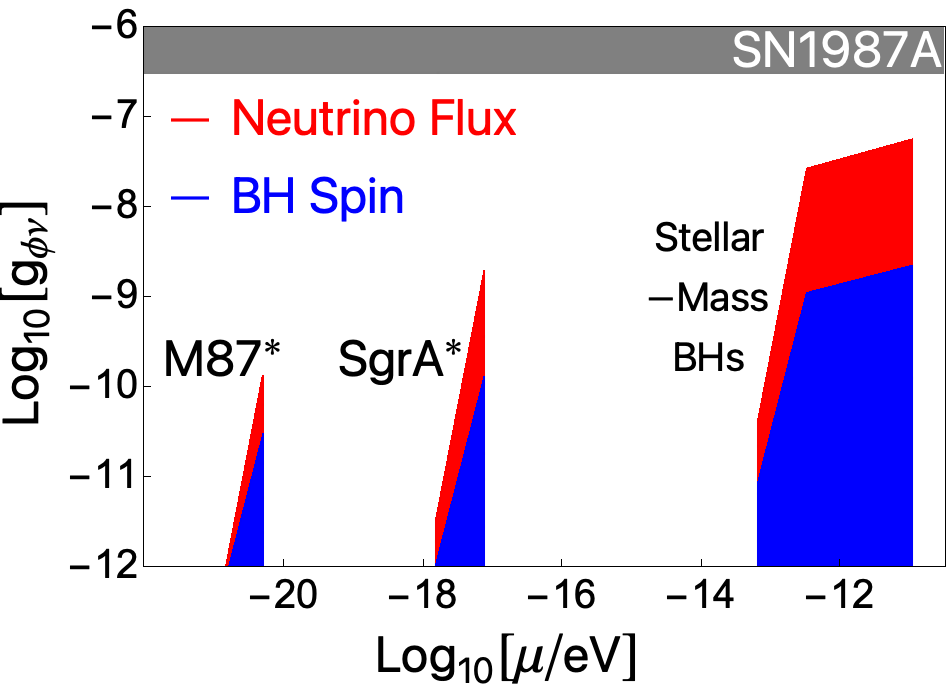
When the interaction between and neutrinos is extremely weak, a steady state is not reached before the BH spins down. Consequently, detecting a BH with a high spin can rule out the corresponding superradiant window mass, similar to the constraints imposed on minimally coupled bosons or axions with weak self-interaction Arvanitaki and Dubovsky (2011); Arvanitaki et al. (2015); Brito et al. (2015b); Baryakhtar et al. (2017); Brito et al. (2017a); Cardoso et al. (2018); Davoudiasl and Denton (2019); Brito et al. (2020); Stott (2020); Ünal et al. (2021); Saha et al. (2022). A quantitative criterion for this exclusion is that , which implies that the cloud extracts of the BH energy without reaching the saturation phase. The blue region in Fig. 2 represents this condition. In our analysis, we consider a fixed spin parameter with the highest possible value of . The lower bound of is set at . For stellar-mass BHs, the corresponding scalar mass , is divided into two regions. In the low-mass region, we fix and vary from to . In the high-mass region, we fix and vary from to . We also include the constraints from the two nearby supermassive BHs.
The parameter space within the red region in Fig. 2 represents the range in which observable neutrino fluxes from a saturating cloud are expected. In this region, the cloud no longer exponentially extracts BH spin, thus enabling the coexistence of a high spin BH and the saturated cloud. Therefore, we maintain the value of , while follows the same division as the one used for spin measurement. The upper boundary of the blue region is determined by requiring the neutrino fluxes in Eq. (7) to be higher than of the diffusive atmospheric neutrino background Vitagliano et al. (2020) at . The atmospheric neutrino has already been well measured by IceCube Aartsen et al. (2015), Super-Kamiokande Richard et al. (2016), ANTARES Albert et al. (2018), and Baikal-GVD Allakhverdyan et al. (2023). A target source with neutrino fluxes at of the diffusive background can be easily distinguished with an angular resolution of Aartsen et al. (2014); Aiello et al. (2019); Aartsen et al. (2019, 2021); Fiorillo et al. (2023); Abbasi et al. (2023).
V Discussion.
Various intriguing phenomena can arise in the region of strong fields, particularly related to particle production. These phenomena have been previously examined in the preheating stage of the early universe Zeldovich and Starobinsky (1971); Kofman et al. (1997); Greene and Kofman (1999, 2000) and in the context of strong field quantum electrodynamics Schwinger (1951); Grib et al. (1994). Rotating BHs provide an excellent platform for studying particle production, as superradiant clouds can reach field values close to the Planck scale.
In this study, we propose a novel approach to investigate the interaction between ultralight bosonic fields and neutrinos through BH superradiance. Superradiant scalar clouds play dual roles in the generation and acceleration of neutrinos, necessitating both periodic oscillation and spatial gradient of the cloud wave-functions. The observation prospects can be examined from two perspectives. First, BH spin measurements can exclude negligible interactions with low values of . Second, neutrino fluxes from a target BH with high spin can constrain the region of strong interaction. Our findings demonstrate that the emitted neutrino fluxes can significantly surpass the diffusive background, both for stellar-mass BHs and supermassive BHs.
Apart from interactions involving a hidden scalar, it is also natural to consider interactions with a vector field in the presence of new gauge groups Georgi and Glashow (1974); Pati and Salam (1974); Mohapatra and Pati (1975); Fritzsch and Minkowski (1975); Georgi (1975). The vector cloud can generate neutrinos through Schwinger pair production Schwinger (1951); Grib et al. (1994) and further accelerate them using the electric fields of the vector. However, the couplings between vector fields and neutrinos are subject to strict constraints due to their coupling to other standard model fermions Graham et al. (2016); Pierce et al. (2018); Abbott et al. (2022b); Shaw et al. (2022); Xue et al. (2022); Ge and Pasquini (2022); Yu et al. (2023) or the non-conservation of currents Laha et al. (2014); Bakhti and Farzan (2017); Escudero et al. (2019); Bahraminasr et al. (2021); Dror (2020); Ekhterachian et al. (2021); Singh et al. (2023). Thus sophisticated model building is necessary in the neutrino sector to yield observable consequences.
Notice that the neutrino production from a bosonic cloud can also apply to other coupled fermions in the hidden sector. In addition, dark matter particles around the cloud can be directly accelerated to higher energies. Consequently the superradiant cloud can serve as a source for boosted dark matter, offering potential for detection through direct detection experiments and neutrino detectors D’Eramo and Thaler (2010); Huang and Zhao (2014); Agashe et al. (2014); Kopp et al. (2015); Bhattacharya et al. (2017); Kamada et al. (2018a); Kachulis et al. (2018); Chatterjee et al. (2018); Kamada et al. (2018b); McKeen and Raj (2019); Argüelles et al. (2020); Kamada and Kim (2020); Berger et al. (2021); Abi et al. (2020). The specific incoming directions of these particles can induce a daily modulation of signals due to scattering with Earth materials Ge et al. (2021); Fornal et al. (2020); Chen et al. (2023b); Xia et al. (2022); Cui et al. (2022); Qiao et al. (2023) or directional detectors Vahsen et al. (2021).
Acknowledgements.
We are grateful to Mauricio Bustamante, Yuxin Liu, and Xin Wang for useful discussions. This work is supported by VILLUM FONDEN (grant no. 37766), by the Danish Research Foundation, and under the European Union’s H2020 ERC Advanced Grant “Black holes: gravitational engines of discovery” grant agreement no. Gravitas–101052587. X.X. is supported by Deutsche Forschungsgemeinschaft under Germany’s Excellence Strategy EXC2121 “Quantum Universe” - 390833306. Views and opinions expressed are however those of the author only and do not necessarily reflect those of the European Union or the European Research Council. Neither the European Union nor the granting authority can be held responsible for them. This work was supported by FCT (Fundação para a Ciência e Tecnologia I.P, Portugal) under project No. 2022.01324.PTDC. This project has received funding from the European Union’s Horizon 2020 research and innovation programme under the Marie Sklodowska-Curie grant agreement No 101007855.References
- Peccei and Quinn (1977) R. D. Peccei and Helen R. Quinn, “CP Conservation in the Presence of Instantons,” Phys. Rev. Lett. 38, 1440–1443 (1977).
- Svrcek and Witten (2006) Peter Svrcek and Edward Witten, “Axions In String Theory,” JHEP 06, 051 (2006), arXiv:hep-th/0605206 .
- Abel et al. (2008) S. A. Abel, M. D. Goodsell, J. Jaeckel, V. V. Khoze, and A. Ringwald, “Kinetic Mixing of the Photon with Hidden U(1)s in String Phenomenology,” JHEP 07, 124 (2008), arXiv:0803.1449 [hep-ph] .
- Arvanitaki et al. (2010) Asimina Arvanitaki, Savas Dimopoulos, Sergei Dubovsky, Nemanja Kaloper, and John March-Russell, “String Axiverse,” Phys. Rev. D81, 123530 (2010), arXiv:0905.4720 [hep-th] .
- Goodsell et al. (2009) Mark Goodsell, Joerg Jaeckel, Javier Redondo, and Andreas Ringwald, “Naturally Light Hidden Photons in LARGE Volume String Compactifications,” JHEP 11, 027 (2009), arXiv:0909.0515 [hep-ph] .
- Preskill et al. (1983) John Preskill, Mark B. Wise, and Frank Wilczek, “Cosmology of the Invisible Axion,” Phys. Lett. 120B, 127–132 (1983).
- Abbott and Sikivie (1983) L. F. Abbott and P. Sikivie, “A Cosmological Bound on the Invisible Axion,” Phys. Lett. B 120, 133–136 (1983).
- Dine and Fischler (1983) Michael Dine and Willy Fischler, “The Not So Harmless Axion,” Phys. Lett. B 120, 137–141 (1983).
- Nelson and Scholtz (2011) Ann E. Nelson and Jakub Scholtz, “Dark Light, Dark Matter and the Misalignment Mechanism,” Phys. Rev. D 84, 103501 (2011), arXiv:1105.2812 [hep-ph] .
- Hu et al. (2000) Wayne Hu, Rennan Barkana, and Andrei Gruzinov, “Cold and fuzzy dark matter,” Phys. Rev. Lett. 85, 1158–1161 (2000), arXiv:astro-ph/0003365 .
- Penrose and Floyd (1971) R. Penrose and R. M. Floyd, “Extraction of rotational energy from a black hole,” Nature 229, 177–179 (1971).
- Zel’Dovich (1971) Ya. B. Zel’Dovich, “Generation of Waves by a Rotating Body,” Soviet Journal of Experimental and Theoretical Physics Letters 14, 180 (1971).
- Brito et al. (2015a) Richard Brito, Vitor Cardoso, and Paolo Pani, “Superradiance: New Frontiers in Black Hole Physics,” Lect. Notes Phys. 906, pp.1–237 (2015a), arXiv:1501.06570 [gr-qc] .
- Detweiler (1980) Steven L. Detweiler, “KLEIN-GORDON EQUATION AND ROTATING BLACK HOLES,” Phys. Rev. D 22, 2323–2326 (1980).
- Cardoso and Yoshida (2005) Vitor Cardoso and Shijun Yoshida, “Superradiant instabilities of rotating black branes and strings,” JHEP 07, 009 (2005), arXiv:hep-th/0502206 .
- Dolan (2007) Sam R. Dolan, “Instability of the massive Klein-Gordon field on the Kerr spacetime,” Phys. Rev. D 76, 084001 (2007), arXiv:0705.2880 [gr-qc] .
- Brito et al. (2015b) Richard Brito, Vitor Cardoso, and Paolo Pani, “Black holes as particle detectors: evolution of superradiant instabilities,” Class. Quant. Grav. 32, 134001 (2015b), arXiv:1411.0686 [gr-qc] .
- East and Pretorius (2017) William E. East and Frans Pretorius, “Superradiant Instability and Backreaction of Massive Vector Fields around Kerr Black Holes,” Phys. Rev. Lett. 119, 041101 (2017), arXiv:1704.04791 [gr-qc] .
- Herdeiro et al. (2022) Carlos A. R. Herdeiro, Eugen Radu, and Nuno M. Santos, “A bound on energy extraction (and hairiness) from superradiance,” Phys. Lett. B 824, 136835 (2022), arXiv:2111.03667 [gr-qc] .
- Chen et al. (2023a) Yifan Chen, Xiao Xue, Richard Brito, and Vitor Cardoso, “Photon Ring Astrometry for Superradiant Clouds,” Phys. Rev. Lett. 130, 111401 (2023a), arXiv:2211.03794 [gr-qc] .
- Arvanitaki and Dubovsky (2011) Asimina Arvanitaki and Sergei Dubovsky, “Exploring the String Axiverse with Precision Black Hole Physics,” Phys. Rev. D83, 044026 (2011), arXiv:1004.3558 [hep-th] .
- Arvanitaki et al. (2015) Asimina Arvanitaki, Masha Baryakhtar, and Xinlu Huang, “Discovering the QCD Axion with Black Holes and Gravitational Waves,” Phys. Rev. D91, 084011 (2015), arXiv:1411.2263 [hep-ph] .
- Baryakhtar et al. (2017) Masha Baryakhtar, Robert Lasenby, and Mae Teo, “Black Hole Superradiance Signatures of Ultralight Vectors,” Phys. Rev. D 96, 035019 (2017), arXiv:1704.05081 [hep-ph] .
- Brito et al. (2017a) Richard Brito, Shrobana Ghosh, Enrico Barausse, Emanuele Berti, Vitor Cardoso, Irina Dvorkin, Antoine Klein, and Paolo Pani, “Gravitational wave searches for ultralight bosons with LIGO and LISA,” Phys. Rev. D 96, 064050 (2017a), arXiv:1706.06311 [gr-qc] .
- Cardoso et al. (2018) Vitor Cardoso, Óscar J. C. Dias, Gavin S. Hartnett, Matthew Middleton, Paolo Pani, and Jorge E. Santos, “Constraining the mass of dark photons and axion-like particles through black-hole superradiance,” JCAP 03, 043 (2018), arXiv:1801.01420 [gr-qc] .
- Davoudiasl and Denton (2019) Hooman Davoudiasl and Peter B Denton, “Ultralight Boson Dark Matter and Event Horizon Telescope Observations of M87*,” Phys. Rev. Lett. 123, 021102 (2019), arXiv:1904.09242 [astro-ph.CO] .
- Brito et al. (2020) Richard Brito, Sara Grillo, and Paolo Pani, “Black Hole Superradiant Instability from Ultralight Spin-2 Fields,” Phys. Rev. Lett. 124, 211101 (2020), arXiv:2002.04055 [gr-qc] .
- Stott (2020) Matthew J. Stott, “Ultralight Bosonic Field Mass Bounds from Astrophysical Black Hole Spin,” (2020), arXiv:2009.07206 [hep-ph] .
- Ünal et al. (2021) Caner Ünal, Fabio Pacucci, and Abraham Loeb, “Properties of ultralight bosons from heavy quasar spins via superradiance,” JCAP 05, 007 (2021), arXiv:2012.12790 [hep-ph] .
- Saha et al. (2022) Akash Kumar Saha, Priyank Parashari, Tarak Nath Maity, Abhishek Dubey, Subhadip Bouri, and Ranjan Laha, “Bounds on ultralight bosons from the Event Horizon Telescope observation of Sgr A∗,” (2022), arXiv:2208.03530 [astro-ph.HE] .
- Yoshino and Kodama (2012) Hirotaka Yoshino and Hideo Kodama, “Bosenova collapse of axion cloud around a rotating black hole,” Prog. Theor. Phys. 128, 153–190 (2012), arXiv:1203.5070 [gr-qc] .
- Yoshino and Kodama (2014) Hirotaka Yoshino and Hideo Kodama, “Gravitational radiation from an axion cloud around a black hole: Superradiant phase,” PTEP 2014, 043E02 (2014), arXiv:1312.2326 [gr-qc] .
- Yoshino and Kodama (2015) Hirotaka Yoshino and Hideo Kodama, “The bosenova and axiverse,” Class. Quant. Grav. 32, 214001 (2015), arXiv:1505.00714 [gr-qc] .
- Brito et al. (2017b) Richard Brito, Shrobana Ghosh, Enrico Barausse, Emanuele Berti, Vitor Cardoso, Irina Dvorkin, Antoine Klein, and Paolo Pani, “Stochastic and resolvable gravitational waves from ultralight bosons,” Phys. Rev. Lett. 119, 131101 (2017b), arXiv:1706.05097 [gr-qc] .
- Isi et al. (2019) Maximiliano Isi, Ling Sun, Richard Brito, and Andrew Melatos, “Directed searches for gravitational waves from ultralight bosons,” Phys. Rev. D 99, 084042 (2019), [Erratum: Phys.Rev.D 102, 049901 (2020)], arXiv:1810.03812 [gr-qc] .
- Siemonsen and East (2020) Nils Siemonsen and William E. East, “Gravitational wave signatures of ultralight vector bosons from black hole superradiance,” Phys. Rev. D 101, 024019 (2020), arXiv:1910.09476 [gr-qc] .
- Sun et al. (2020) Ling Sun, Richard Brito, and Maximiliano Isi, “Search for ultralight bosons in Cygnus X-1 with Advanced LIGO,” Phys. Rev. D 101, 063020 (2020), [Erratum: Phys.Rev.D 102, 089902 (2020)], arXiv:1909.11267 [gr-qc] .
- Palomba et al. (2019) Cristiano Palomba et al., “Direct constraints on ultra-light boson mass from searches for continuous gravitational waves,” Phys. Rev. Lett. 123, 171101 (2019), arXiv:1909.08854 [astro-ph.HE] .
- Zhu et al. (2020) Sylvia J. Zhu, Masha Baryakhtar, Maria Alessandra Papa, Daichi Tsuna, Norita Kawanaka, and Heinz-Bernd Eggenstein, “Characterizing the continuous gravitational-wave signal from boson clouds around Galactic isolated black holes,” Phys. Rev. D 102, 063020 (2020), arXiv:2003.03359 [gr-qc] .
- Tsukada et al. (2021) Leo Tsukada, Richard Brito, William E. East, and Nils Siemonsen, “Modeling and searching for a stochastic gravitational-wave background from ultralight vector bosons,” Phys. Rev. D 103, 083005 (2021), arXiv:2011.06995 [astro-ph.HE] .
- Yuan et al. (2021a) Chen Yuan, Richard Brito, and Vitor Cardoso, “Probing ultralight dark matter with future ground-based gravitational-wave detectors,” Phys. Rev. D 104, 044011 (2021a), arXiv:2106.00021 [gr-qc] .
- Abbott et al. (2022a) R. Abbott et al. (KAGRA, VIRGO, LIGO Scientific), “All-sky search for gravitational wave emission from scalar boson clouds around spinning black holes in LIGO O3 data,” Phys. Rev. D 105, 102001 (2022a), arXiv:2111.15507 [astro-ph.HE] .
- Yuan et al. (2022) Chen Yuan, Yang Jiang, and Qing-Guo Huang, “Constraints on an ultralight scalar boson from Advanced LIGO and Advanced Virgo’s first three observing runs using the stochastic gravitational-wave background,” Phys. Rev. D 106, 023020 (2022), arXiv:2204.03482 [astro-ph.CO] .
- Brito and Shah (2023) Richard Brito and Shreya Shah, “Extreme mass-ratio inspirals into black holes surrounded by scalar clouds,” (2023), arXiv:2307.16093 [gr-qc] .
- Chen et al. (2020) Yifan Chen, Jing Shu, Xiao Xue, Qiang Yuan, and Yue Zhao, “Probing Axions with Event Horizon Telescope Polarimetric Measurements,” Phys. Rev. Lett. 124, 061102 (2020), arXiv:1905.02213 [hep-ph] .
- Yuan et al. (2021b) Guan-Wen Yuan, Zi-Qing Xia, Chengfeng Tang, Yaqi Zhao, Yi-Fu Cai, Yifan Chen, Jing Shu, and Qiang Yuan, “Testing the ALP-photon coupling with polarization measurements of Sagittarius A⋆,” JCAP 03, 018 (2021b), arXiv:2008.13662 [astro-ph.HE] .
- Chen et al. (2022a) Yifan Chen, Yuxin Liu, Ru-Sen Lu, Yosuke Mizuno, Jing Shu, Xiao Xue, Qiang Yuan, and Yue Zhao, “Stringent axion constraints with Event Horizon Telescope polarimetric measurements of M87⋆,” Nature Astron. 6, 592–598 (2022a), arXiv:2105.04572 [hep-ph] .
- Chen et al. (2022b) Yifan Chen, Chunlong Li, Yosuke Mizuno, Jing Shu, Xiao Xue, Qiang Yuan, Yue Zhao, and Zihan Zhou, “Birefringence tomography for axion cloud,” JCAP 09, 073 (2022b), arXiv:2208.05724 [hep-ph] .
- Gelmini and Roncadelli (1981) G. B. Gelmini and M. Roncadelli, “Left-Handed Neutrino Mass Scale and Spontaneously Broken Lepton Number,” Phys. Lett. B 99, 411–415 (1981).
- Chikashige et al. (1981) Y. Chikashige, Rabindra N. Mohapatra, and R. D. Peccei, “Are There Real Goldstone Bosons Associated with Broken Lepton Number?” Phys. Lett. B 98, 265–268 (1981).
- Aulakh and Mohapatra (1982) C. S. Aulakh and Rabindra N. Mohapatra, “Neutrino as the Supersymmetric Partner of the Majoron,” Phys. Lett. B 119, 136–140 (1982).
- Georgi and Glashow (1974) H. Georgi and S. L. Glashow, “Unity of All Elementary Particle Forces,” Phys. Rev. Lett. 32, 438–441 (1974).
- Pati and Salam (1974) Jogesh C. Pati and Abdus Salam, “Lepton Number as the Fourth Color,” Phys. Rev. D 10, 275–289 (1974), [Erratum: Phys.Rev.D 11, 703–703 (1975)].
- Mohapatra and Pati (1975) Rabindra N. Mohapatra and Jogesh C. Pati, “Left-Right Gauge Symmetry and an Isoconjugate Model of CP Violation,” Phys. Rev. D 11, 566–571 (1975).
- Fritzsch and Minkowski (1975) Harald Fritzsch and Peter Minkowski, “Unified Interactions of Leptons and Hadrons,” Annals Phys. 93, 193–266 (1975).
- Georgi (1975) Howard Georgi, “The State of the Art—Gauge Theories,” AIP Conf. Proc. 23, 575–582 (1975).
- Kolb and Turner (1987) Edward W. Kolb and Michael S. Turner, “Supernova SN 1987a and the Secret Interactions of Neutrinos,” Phys. Rev. D 36, 2895 (1987).
- Huang et al. (2018) Guo-yuan Huang, Tommy Ohlsson, and Shun Zhou, “Observational Constraints on Secret Neutrino Interactions from Big Bang Nucleosynthesis,” Phys. Rev. D 97, 075009 (2018), arXiv:1712.04792 [hep-ph] .
- Brune and Päs (2019) Tim Brune and Heinrich Päs, “Massive Majorons and constraints on the Majoron-neutrino coupling,” Phys. Rev. D 99, 096005 (2019), arXiv:1808.08158 [hep-ph] .
- Forastieri et al. (2019) Francesco Forastieri, Massimiliano Lattanzi, and Paolo Natoli, “Cosmological constraints on neutrino self-interactions with a light mediator,” Phys. Rev. D 100, 103526 (2019), arXiv:1904.07810 [astro-ph.CO] .
- Berryman et al. (2022) Jeffrey M. Berryman et al., “Neutrino Self-Interactions: A White Paper,” in Snowmass 2021 (2022) arXiv:2203.01955 [hep-ph] .
- Li and Xu (2023) Shao-Ping Li and Xun-Jie Xu, “ constraints on light mediators coupled to neutrinos: the dilution-resistant effect,” (2023), arXiv:2307.13967 [hep-ph] .
- Reynoso and Sampayo (2016) Matías M. Reynoso and Oscar A. Sampayo, “Propagation of high-energy neutrinos in a background of ultralight scalar dark matter,” Astropart. Phys. 82, 10–20 (2016), arXiv:1605.09671 [hep-ph] .
- Berlin (2016) Asher Berlin, “Neutrino Oscillations as a Probe of Light Scalar Dark Matter,” Phys. Rev. Lett. 117, 231801 (2016), arXiv:1608.01307 [hep-ph] .
- Krnjaic et al. (2018) Gordan Krnjaic, Pedro A. N. Machado, and Lina Necib, “Distorted neutrino oscillations from time varying cosmic fields,” Phys. Rev. D 97, 075017 (2018), arXiv:1705.06740 [hep-ph] .
- Brdar et al. (2018) Vedran Brdar, Joachim Kopp, Jia Liu, Pascal Prass, and Xiao-Ping Wang, “Fuzzy dark matter and nonstandard neutrino interactions,” Phys. Rev. D 97, 043001 (2018), arXiv:1705.09455 [hep-ph] .
- Davoudiasl et al. (2018) Hooman Davoudiasl, Gopolang Mohlabeng, and Matthew Sullivan, “Galactic Dark Matter Population as the Source of Neutrino Masses,” Phys. Rev. D 98, 021301 (2018), arXiv:1803.00012 [hep-ph] .
- Liao et al. (2018) Jiajun Liao, Danny Marfatia, and Kerry Whisnant, “Light scalar dark matter at neutrino oscillation experiments,” JHEP 04, 136 (2018), arXiv:1803.01773 [hep-ph] .
- Capozzi et al. (2018) Francesco Capozzi, Ian M. Shoemaker, and Luca Vecchi, “Neutrino Oscillations in Dark Backgrounds,” JCAP 07, 004 (2018), arXiv:1804.05117 [hep-ph] .
- Huang and Nath (2018) Guo-Yuan Huang and Newton Nath, “Neutrinophilic Axion-Like Dark Matter,” Eur. Phys. J. C 78, 922 (2018), arXiv:1809.01111 [hep-ph] .
- Farzan (2019) Yasaman Farzan, “Ultra-light scalar saving the 3 + 1 neutrino scheme from the cosmological bounds,” Phys. Lett. B 797, 134911 (2019), arXiv:1907.04271 [hep-ph] .
- Cline (2020) James M. Cline, “Viable secret neutrino interactions with ultralight dark matter,” Phys. Lett. B 802, 135182 (2020), arXiv:1908.02278 [hep-ph] .
- Dev et al. (2021) Abhish Dev, Pedro A. N. Machado, and Pablo Martínez-Miravé, “Signatures of ultralight dark matter in neutrino oscillation experiments,” JHEP 01, 094 (2021), arXiv:2007.03590 [hep-ph] .
- Losada et al. (2022) Marta Losada, Yosef Nir, Gilad Perez, and Yogev Shpilman, “Probing scalar dark matter oscillations with neutrino oscillations,” JHEP 04, 030 (2022), arXiv:2107.10865 [hep-ph] .
- Huang and Nath (2022) Guo-yuan Huang and Newton Nath, “Neutrino meets ultralight dark matter: 0 decay and cosmology,” JCAP 05, 034 (2022), arXiv:2111.08732 [hep-ph] .
- Chun (2021) Eung Jin Chun, “Neutrino Transition in Dark Matter,” (2021), arXiv:2112.05057 [hep-ph] .
- Dev et al. (2023) Abhish Dev, Gordan Krnjaic, Pedro Machado, and Harikrishnan Ramani, “Constraining feeble neutrino interactions with ultralight dark matter,” Phys. Rev. D 107, 035006 (2023), arXiv:2205.06821 [hep-ph] .
- Losada et al. (2023a) Marta Losada, Yosef Nir, Gilad Perez, Inbar Savoray, and Yogev Shpilman, “Parametric resonance in neutrino oscillations induced by ultra-light dark matter and implications for KamLAND and JUNO,” JHEP 03, 032 (2023a), arXiv:2205.09769 [hep-ph] .
- Brzeminski et al. (2022) Dawid Brzeminski, Saurav Das, Anson Hook, and Clayton Ristow, “Constraining Vector Dark Matter with Neutrino experiments,” (2022), arXiv:2212.05073 [hep-ph] .
- Alonso-Álvarez et al. (2023) Gonzalo Alonso-Álvarez, Katarina Bleau, and James M. Cline, “Distortion of neutrino oscillations by dark photon dark matter,” Phys. Rev. D 107, 055045 (2023), arXiv:2301.04152 [hep-ph] .
- ChoeJo et al. (2023) YeolLin ChoeJo, Yechan Kim, and Hye-Sung Lee, “Dirac-Majorana neutrino type conversion induced by an oscillating scalar dark matter,” (2023), arXiv:2305.16900 [hep-ph] .
- Losada et al. (2023b) Marta Losada, Yosef Nir, Gilad Perez, Inbar Savoray, and Yogev Shpilman, “Time Dependent CP-even and CP-odd Signatures of Scalar Ultra-light Dark Matter in Neutrino Oscillations,” (2023b), arXiv:2302.00005 [hep-ph] .
- Greene and Kofman (1999) Patrick B. Greene and Lev Kofman, “Preheating of fermions,” Phys. Lett. B 448, 6–12 (1999), arXiv:hep-ph/9807339 .
- Greene and Kofman (2000) Patrick B. Greene and Lev Kofman, “On the theory of fermionic preheating,” Phys. Rev. D 62, 123516 (2000), arXiv:hep-ph/0003018 .
- Vitagliano et al. (2020) Edoardo Vitagliano, Irene Tamborra, and Georg Raffelt, “Grand Unified Neutrino Spectrum at Earth: Sources and Spectral Components,” Rev. Mod. Phys. 92, 45006 (2020), arXiv:1910.11878 [astro-ph.HE] .
- Fukuda and Nakayama (2020) Hajime Fukuda and Kazunori Nakayama, “Aspects of Nonlinear Effect on Black Hole Superradiance,” JHEP 01, 128 (2020), arXiv:1910.06308 [hep-ph] .
- Baryakhtar et al. (2021) Masha Baryakhtar, Marios Galanis, Robert Lasenby, and Olivier Simon, “Black hole superradiance of self-interacting scalar fields,” Phys. Rev. D 103, 095019 (2021), arXiv:2011.11646 [hep-ph] .
- Omiya et al. (2022) Hidetoshi Omiya, Takuya Takahashi, Takahiro Tanaka, and Hirotaka Yoshino, “Impact of multiple modes on the evolution of self-interacting axion condensate around rotating black holes,” (2022), arXiv:2211.01949 [gr-qc] .
- Rosa and Kephart (2018) João G. Rosa and Thomas W. Kephart, “Stimulated Axion Decay in Superradiant Clouds around Primordial Black Holes,” Phys. Rev. Lett. 120, 231102 (2018), arXiv:1709.06581 [gr-qc] .
- Boskovic et al. (2019) Mateja Boskovic, Richard Brito, Vitor Cardoso, Taishi Ikeda, and Helvi Witek, “Axionic instabilities and new black hole solutions,” Phys. Rev. D 99, 035006 (2019), arXiv:1811.04945 [gr-qc] .
- Ikeda et al. (2019) Taishi Ikeda, Richard Brito, and Vitor Cardoso, “Blasts of Light from Axions,” Phys. Rev. Lett. 122, 081101 (2019), arXiv:1811.04950 [gr-qc] .
- Spieksma et al. (2023) Thomas F. M. Spieksma, Enrico Cannizzaro, Taishi Ikeda, Vitor Cardoso, and Yifan Chen, “Superradiance: Axionic Couplings and Plasma Effects,” (2023), arXiv:2306.16447 [gr-qc] .
- Blas and Witte (2020) Diego Blas and Samuel J. Witte, “Quenching Mechanisms of Photon Superradiance,” Phys. Rev. D 102, 123018 (2020), arXiv:2009.10075 [hep-ph] .
- Siemonsen et al. (2023) Nils Siemonsen, Cristina Mondino, Daniel Egana-Ugrinovic, Junwu Huang, Masha Baryakhtar, and William E. East, “Dark photon superradiance: Electrodynamics and multimessenger signals,” Phys. Rev. D 107, 075025 (2023), arXiv:2212.09772 [astro-ph.HE] .
- Kachelriess et al. (2000) M. Kachelriess, R. Tomas, and J. W. F. Valle, “Supernova bounds on Majoron emitting decays of light neutrinos,” Phys. Rev. D 62, 023004 (2000), arXiv:hep-ph/0001039 .
- Farzan (2003) Yasaman Farzan, “Bounds on the coupling of the Majoron to light neutrinos from supernova cooling,” Phys. Rev. D 67, 073015 (2003), arXiv:hep-ph/0211375 .
- Gando et al. (2012) A. Gando et al. (KamLAND-Zen), “Limits on Majoron-emitting double-beta decays of Xe-136 in the KamLAND-Zen experiment,” Phys. Rev. C 86, 021601 (2012), arXiv:1205.6372 [hep-ex] .
- Aghanim et al. (2020) N. Aghanim et al. (Planck), “Planck 2018 results. VI. Cosmological parameters,” Astron. Astrophys. 641, A6 (2020), [Erratum: Astron.Astrophys. 652, C4 (2021)], arXiv:1807.06209 [astro-ph.CO] .
- Singh and Mirza (2023) Jyotsna Singh and M. Ibrahim Mirza, “Challenges in Neutrino Mass Measurements,” (2023), arXiv:2305.12654 [hep-ex] .
- Uzan et al. (2020) Jean-Philippe Uzan, Martin Pernot-Borràs, and Joel Bergé, “Effects of a scalar fifth force on the dynamics of a charged particle as a new experimental design to test chameleon theories,” Phys. Rev. D 102, 044059 (2020), arXiv:2006.03359 [gr-qc] .
- Berlin and Hook (2020) Asher Berlin and Anson Hook, “Searching for Millicharged Particles with Superconducting Radio-Frequency Cavities,” Phys. Rev. D 102, 035010 (2020), arXiv:2001.02679 [hep-ph] .
- Lewin et al. (1997) Walter H. G. Lewin, Jan van Paradijs, and Edward Peter Jacobus van den Heuvel, X-ray Binaries (1997).
- Brenneman and Reynolds (2006) Laura W. Brenneman and Christopher S. Reynolds, “Constraining Black Hole Spin Via X-ray Spectroscopy,” Astrophys. J. 652, 1028–1043 (2006), arXiv:astro-ph/0608502 .
- Mao et al. (2002) Shude Mao, Martin C. Smith, P. Wozniak, A. Udalski, M. Szymanski M. Kubiak, G. Pietrzynski, I. Soszynski, and K. Zebrun, “Optical gravitational lensing experiment. ogle-1999-bul-32: the longest ever microlensing event - evidence for a stellar mass black hole?” Mon. Not. Roy. Astron. Soc. 329, 349 (2002), arXiv:astro-ph/0108312 .
- Bennett et al. (2002) D. P. Bennett et al., “Gravitational microlensing events due to stellar mass black holes,” Astrophys. J. 579, 639–659 (2002), arXiv:astro-ph/0109467 .
- Barack et al. (2019) Leor Barack et al., “Black holes, gravitational waves and fundamental physics: a roadmap,” Class. Quant. Grav. 36, 143001 (2019), arXiv:1806.05195 [gr-qc] .
- Akiyama et al. (2019) Kazunori Akiyama et al. (Event Horizon Telescope), “First M87 Event Horizon Telescope Results. I. The Shadow of the Supermassive Black Hole,” Astrophys. J. Lett. 875, L1 (2019), arXiv:1906.11238 [astro-ph.GA] .
- Akiyama et al. (2022) Kazunori Akiyama et al. (Event Horizon Telescope), “First Sagittarius A* Event Horizon Telescope Results. I. The Shadow of the Supermassive Black Hole in the Center of the Milky Way,” Astrophys. J. Lett. 930, L12 (2022).
- Kovalev et al. (2023) Y. Y. Kovalev, A. V. Plavin, A. B. Pushkarev, and S. V. Troitsky, “Probing neutrino production in blazars by millimeter VLBI,” Galaxies 11, 84 (2023), arXiv:2307.02267 [astro-ph.HE] .
- Aartsen et al. (2015) M. G. Aartsen et al. (IceCube), “Measurement of the Atmospheric Spectrum with IceCube,” Phys. Rev. D 91, 122004 (2015), arXiv:1504.03753 [astro-ph.HE] .
- Richard et al. (2016) E. Richard et al. (Super-Kamiokande), “Measurements of the atmospheric neutrino flux by Super-Kamiokande: energy spectra, geomagnetic effects, and solar modulation,” Phys. Rev. D 94, 052001 (2016), arXiv:1510.08127 [hep-ex] .
- Albert et al. (2018) A. Albert et al. (ANTARES), “All-flavor Search for a Diffuse Flux of Cosmic Neutrinos with Nine Years of ANTARES Data,” Astrophys. J. Lett. 853, L7 (2018), arXiv:1711.07212 [astro-ph.HE] .
- Allakhverdyan et al. (2023) V. A. Allakhverdyan et al. (Baikal-GVD), “Diffuse neutrino flux measurements with the Baikal-GVD neutrino telescope,” Phys. Rev. D 107, 042005 (2023), arXiv:2211.09447 [astro-ph.HE] .
- Aartsen et al. (2014) M. G. Aartsen et al. (IceCube), “Energy Reconstruction Methods in the IceCube Neutrino Telescope,” JINST 9, P03009 (2014), arXiv:1311.4767 [physics.ins-det] .
- Aiello et al. (2019) S. Aiello et al. (KM3NeT), “Sensitivity of the KM3NeT/ARCA neutrino telescope to point-like neutrino sources,” Astropart. Phys. 111, 100–110 (2019), arXiv:1810.08499 [astro-ph.HE] .
- Aartsen et al. (2019) M. G. Aartsen et al. (IceCube), “Search for steady point-like sources in the astrophysical muon neutrino flux with 8 years of IceCube data,” Eur. Phys. J. C 79, 234 (2019), arXiv:1811.07979 [hep-ph] .
- Aartsen et al. (2021) M. G. Aartsen et al. (IceCube-Gen2), “IceCube-Gen2: the window to the extreme Universe,” J. Phys. G 48, 060501 (2021), arXiv:2008.04323 [astro-ph.HE] .
- Fiorillo et al. (2023) Damiano F. G. Fiorillo, Mauricio Bustamante, and Victor B. Valera, “Near-future discovery of point sources of ultra-high-energy neutrinos,” JCAP 03, 026 (2023), arXiv:2205.15985 [astro-ph.HE] .
- Abbasi et al. (2023) R. Abbasi et al. (IceCube), “Observation of high-energy neutrinos from the Galactic plane,” Science 380, 6652 (2023), arXiv:2307.04427 [astro-ph.HE] .
- Zeldovich and Starobinsky (1971) Ya. B. Zeldovich and Alexei A. Starobinsky, “Particle production and vacuum polarization in an anisotropic gravitational field,” Zh. Eksp. Teor. Fiz. 61, 2161–2175 (1971).
- Kofman et al. (1997) Lev Kofman, Andrei D. Linde, and Alexei A. Starobinsky, “Towards the theory of reheating after inflation,” Phys. Rev. D 56, 3258–3295 (1997), arXiv:hep-ph/9704452 .
- Schwinger (1951) Julian S. Schwinger, “On gauge invariance and vacuum polarization,” Phys. Rev. 82, 664–679 (1951).
- Grib et al. (1994) A.A. Grib, S.G. Mamayev, V.M. Mostepanenko, and V.M. Mostepanenko, Vacuum Quantum Effects in Strong Fields (Friedmann Laboratory Pub., 1994).
- Graham et al. (2016) Peter W. Graham, David E. Kaplan, Jeremy Mardon, Surjeet Rajendran, and William A. Terrano, “Dark Matter Direct Detection with Accelerometers,” Phys. Rev. D 93, 075029 (2016), arXiv:1512.06165 [hep-ph] .
- Pierce et al. (2018) Aaron Pierce, Keith Riles, and Yue Zhao, “Searching for Dark Photon Dark Matter with Gravitational Wave Detectors,” Phys. Rev. Lett. 121, 061102 (2018), arXiv:1801.10161 [hep-ph] .
- Abbott et al. (2022b) R. Abbott et al. (LIGO Scientific, KAGRA, Virgo), “Constraints on dark photon dark matter using data from LIGO’s and Virgo’s third observing run,” Phys. Rev. D 105, 063030 (2022b), arXiv:2105.13085 [astro-ph.CO] .
- Shaw et al. (2022) E. A. Shaw, M. P. Ross, C. A. Hagedorn, E. G. Adelberger, and J. H. Gundlach, “Torsion-balance search for ultralow-mass bosonic dark matter,” Phys. Rev. D 105, 042007 (2022), arXiv:2109.08822 [astro-ph.CO] .
- Xue et al. (2022) Xiao Xue et al. (PPTA), “High-precision search for dark photon dark matter with the Parkes Pulsar Timing Array,” Phys. Rev. Res. 4, L012022 (2022), arXiv:2112.07687 [hep-ph] .
- Ge and Pasquini (2022) Shao-Feng Ge and Pedro Pasquini, “Probing light mediators in the radiative emission of neutrino pair,” Eur. Phys. J. C 82, 208 (2022), arXiv:2110.03510 [hep-ph] .
- Yu et al. (2023) Jiang-Chuan Yu, Yue-Hui Yao, Yong Tang, and Yue-Liang Wu, “Sensitivity of Space-based Gravitational-Wave Interferometers to Ultralight Bosonic Fields and Dark Matter,” (2023), arXiv:2307.09197 [gr-qc] .
- Laha et al. (2014) Ranjan Laha, Basudeb Dasgupta, and John F. Beacom, “Constraints on New Neutrino Interactions via Light Abelian Vector Bosons,” Phys. Rev. D 89, 093025 (2014), arXiv:1304.3460 [hep-ph] .
- Bakhti and Farzan (2017) Pouya Bakhti and Yasaman Farzan, “Constraining secret gauge interactions of neutrinos by meson decays,” Phys. Rev. D 95, 095008 (2017), arXiv:1702.04187 [hep-ph] .
- Escudero et al. (2019) Miguel Escudero, Dan Hooper, Gordan Krnjaic, and Mathias Pierre, “Cosmology with A Very Light Lμ Lτ Gauge Boson,” JHEP 03, 071 (2019), arXiv:1901.02010 [hep-ph] .
- Bahraminasr et al. (2021) Majid Bahraminasr, Pouya Bakhti, and Meshkat Rajaee, “Sensitivities to secret neutrino interaction at FASER,” J. Phys. G 48, 095001 (2021), arXiv:2003.09985 [hep-ph] .
- Dror (2020) Jeff A. Dror, “Discovering leptonic forces using nonconserved currents,” Phys. Rev. D 101, 095013 (2020), arXiv:2004.04750 [hep-ph] .
- Ekhterachian et al. (2021) Majid Ekhterachian, Anson Hook, Soubhik Kumar, and Yuhsin Tsai, “Bounds on gauge bosons coupled to nonconserved currents,” Phys. Rev. D 104, 035034 (2021), arXiv:2103.13396 [hep-ph] .
- Singh et al. (2023) Masoom Singh, Mauricio Bustamante, and Sanjib Kumar Agarwalla, “Flavor-dependent long-range neutrino interactions in DUNE & T2HK: alone they constrain, together they discover,” (2023), arXiv:2305.05184 [hep-ph] .
- D’Eramo and Thaler (2010) Francesco D’Eramo and Jesse Thaler, “Semi-annihilation of Dark Matter,” JHEP 06, 109 (2010), arXiv:1003.5912 [hep-ph] .
- Huang and Zhao (2014) Junwu Huang and Yue Zhao, “Dark Matter Induced Nucleon Decay: Model and Signatures,” JHEP 02, 077 (2014), arXiv:1312.0011 [hep-ph] .
- Agashe et al. (2014) Kaustubh Agashe, Yanou Cui, Lina Necib, and Jesse Thaler, “(In)direct Detection of Boosted Dark Matter,” JCAP 10, 062 (2014), arXiv:1405.7370 [hep-ph] .
- Kopp et al. (2015) Joachim Kopp, Jia Liu, and Xiao-Ping Wang, “Boosted Dark Matter in IceCube and at the Galactic Center,” JHEP 04, 105 (2015), arXiv:1503.02669 [hep-ph] .
- Bhattacharya et al. (2017) Atri Bhattacharya, Raj Gandhi, Aritra Gupta, and Satyanarayan Mukhopadhyay, “Boosted Dark Matter and its implications for the features in IceCube HESE data,” JCAP 05, 002 (2017), arXiv:1612.02834 [hep-ph] .
- Kamada et al. (2018a) Ayuki Kamada, Hee Jung Kim, Hyungjin Kim, and Toyokazu Sekiguchi, “Self-Heating Dark Matter via Semiannihilation,” Phys. Rev. Lett. 120, 131802 (2018a), arXiv:1707.09238 [hep-ph] .
- Kachulis et al. (2018) C. Kachulis et al. (Super-Kamiokande), “Search for Boosted Dark Matter Interacting With Electrons in Super-Kamiokande,” Phys. Rev. Lett. 120, 221301 (2018), arXiv:1711.05278 [hep-ex] .
- Chatterjee et al. (2018) Animesh Chatterjee, Albert De Roeck, Doojin Kim, Zahra Gh. Moghaddam, Jong-Chul Park, Seodong Shin, Leigh H. Whitehead, and Jaehoon Yu, “Searching for boosted dark matter at ProtoDUNE,” Phys. Rev. D 98, 075027 (2018), arXiv:1803.03264 [hep-ph] .
- Kamada et al. (2018b) Ayuki Kamada, Hee Jung Kim, and Hyungjin Kim, “Self-heating of Strongly Interacting Massive Particles,” Phys. Rev. D 98, 023509 (2018b), arXiv:1805.05648 [hep-ph] .
- McKeen and Raj (2019) David McKeen and Nirmal Raj, “Monochromatic dark neutrinos and boosted dark matter in noble liquid direct detection,” Phys. Rev. D 99, 103003 (2019), arXiv:1812.05102 [hep-ph] .
- Argüelles et al. (2020) C. A. Argüelles et al., “New opportunities at the next-generation neutrino experiments I: BSM neutrino physics and dark matter,” Rept. Prog. Phys. 83, 124201 (2020), arXiv:1907.08311 [hep-ph] .
- Kamada and Kim (2020) Ayuki Kamada and Hee Jung Kim, “Escalating core formation with dark matter self-heating,” Phys. Rev. D 102, 043009 (2020), arXiv:1911.09717 [hep-ph] .
- Berger et al. (2021) Joshua Berger, Yanou Cui, Mathew Graham, Lina Necib, Gianluca Petrillo, Dane Stocks, Yun-Tse Tsai, and Yue Zhao, “Prospects for detecting boosted dark matter in DUNE through hadronic interactions,” Phys. Rev. D 103, 095012 (2021), arXiv:1912.05558 [hep-ph] .
- Abi et al. (2020) Babak Abi et al. (DUNE), “Deep Underground Neutrino Experiment (DUNE), Far Detector Technical Design Report, Volume II: DUNE Physics,” (2020), arXiv:2002.03005 [hep-ex] .
- Ge et al. (2021) Shao-Feng Ge, Jianglai Liu, Qiang Yuan, and Ning Zhou, “Diurnal Effect of Sub-GeV Dark Matter Boosted by Cosmic Rays,” Phys. Rev. Lett. 126, 091804 (2021), arXiv:2005.09480 [hep-ph] .
- Fornal et al. (2020) Bartosz Fornal, Pearl Sandick, Jing Shu, Meng Su, and Yue Zhao, “Boosted Dark Matter Interpretation of the XENON1T Excess,” Phys. Rev. Lett. 125, 161804 (2020), arXiv:2006.11264 [hep-ph] .
- Chen et al. (2023b) Yifan Chen, Bartosz Fornal, Pearl Sandick, Jing Shu, Xiao Xue, Yue Zhao, and Junchao Zong, “Earth shielding and daily modulation from electrophilic boosted dark particles,” Phys. Rev. D 107, 033006 (2023b), arXiv:2110.09685 [hep-ph] .
- Xia et al. (2022) Chen Xia, Yan-Hao Xu, and Yu-Feng Zhou, “Production and attenuation of cosmic-ray boosted dark matter,” JCAP 02, 028 (2022), arXiv:2111.05559 [hep-ph] .
- Cui et al. (2022) Xiangyi Cui et al. (PandaX-II), “Search for Cosmic-Ray Boosted Sub-GeV Dark Matter at the PandaX-II Experiment,” Phys. Rev. Lett. 128, 171801 (2022), arXiv:2112.08957 [hep-ex] .
- Qiao et al. (2023) Mai Qiao, Chen Xia, and Yu-Feng Zhou, “Diurnal modulation of electron recoils from DM-nucleon scattering through the Migdal effect,” (2023), arXiv:2307.12820 [hep-ph] .
- Vahsen et al. (2021) Sven E. Vahsen, Ciaran A. J. O’Hare, and Dinesh Loomba, “Directional Recoil Detection,” Ann. Rev. Nucl. Part. Sci. 71, 189–224 (2021), arXiv:2102.04596 [physics.ins-det] .
- Casella et al. (2004) George Casella, Christian Robert, and Martin Wells, “Generalized accept-reject sampling schemes,” Lecture Notes-Monograph Series 45 (2004), 10.1214/lnms/1196285403.
Supplemental Material: Black Holes as Neutrino Factories
.1 Particle Production from Time-Varying Backgrounds
We begin by considering a bosonic field in a time-varying background Zeldovich and Starobinsky (1971); Kofman et al. (1997). The equation of motion in the frequency domain can be expressed as
| (S1) |
Here, represents the time-varying energy, which is modulated by the background fields to which couples. The solutions to Eq. (S1) in the adiabatic representation are given by Kofman et al. (1997)
| (S2) |
The coefficients and satisfy the following equations:
| (S3) |
and they adhere to the normalization condition . Initially, at , the vacuum state is defined as and . The quantities and correspond to the coefficients of the Bogoliubov transformation of the creation and annihilation operators, respectively, which diagonalize the Hamiltonian at each moment in time . The particle occupation number for a momentum mode is given by , which yields the particle number density per unit volume as
| (S4) |
When holds true, we can approximate the solution for Eq. (S3) as
| (S5) |
Consequently, efficient particle production is expected when the non-adiabatic condition is satisfied:
| (S6) |
Using the interaction term as an example, we consider the following scenario: represents the coherently oscillating background scalar with amplitude and frequency , and represents the coupling constant. The frequency relation for is Kofman et al. (1997)
| (S7) |
Here, denotes the bare mass term of . In this context, our focus lies on the region where is substantially greater than , while can be considered negligible. Within a narrow region of during a single oscillation period, momentum values below the typical scale satisfy the non-adiabatic condition (S6). Consequently, the occupation number for is exponentially produced with a time dependence of approximately , where Kofman et al. (1997).
Fermionic fields with a Yukawa coupling and a bare mass exhibit a frequency relation for the mode function given by Greene and Kofman (1999, 2000)
| (S8) |
In the near black hole region where the resonance parameter is significantly high and , the non-adiabatic condition is met when the effective mass term, , crosses zero. During each crossing, the background ground instantly contributes to the mode with a factor of Greene and Kofman (1999, 2000), where contains the terms related to previously produced fermions. Exponential growth is excluded due to Pauli blocking. Instead, a fermion sphere with a radius of approximately is formed immediately after a single kick. In cases where neutrinos are produced from a superradiant scalar background, neutrinos produced during the previous kick are accelerated to much higher energy scales and will not obstruct subsequent production. Consequently, the average production rate per unit volume is estimated as:
| (S9) |
Here, the factor accounts for the time between two crossings. Furthermore, the de Broglie wavelength of the initially produced fermions, approximately , is considerably shorter than the cloud size. Thus, the finite size of the cloud can be disregarded when considering the production rate.
The scalar cloud displays an oscillatory component in its wavefunction, which exhibits a dependency on the azimuthal angle, i.e., . This dependence arises from the orbital angular momentum of the cloud. Notably, at a specific time , the non-adiabatic condition is triggered on a plane that is approximately aligned with . As a result, the cloud oscillation induces a periodic rotation of the production plane around the spin axis of the black hole.
One key difference between boson and fermion production is the requirement for the bare mass term. In Eq. (S8), the effective mass is the linear sum of the bare mass and the oscillating term, so only is necessary to trigger the parametric excitation Greene and Kofman (2000). On the other hand, for bosons, needs to be smaller than due to their similar roles in Eq. (S8). In our cases, due to the smallness of the neutrino mass and the significant field value of the scalar cloud, neutrino production can be achieved for both stellar-mass black holes and supermassive black holes with different ranges of .
.2 Neutrino Trajectory
Immediately after production, neutrinos start propagating under the scalar background outside the black hole. This is effectively equivalent to considering geodesics with a varying mass term denoted by . The worldline action for the neutrino is given by:
| (S10) |
where is the Kerr metric, and is the -velocity of the neutrino particle. From Eq. (S10), we obtain the corresponding Euler-Lagrange equation:
| (S11) |
where is the proper time, and are the Christoffel symbols of the Kerr metric. By using the relations and , we can rewrite Eq. (S11) as:
| (S12) |
Here, satisfies the on-shell condition . The time-component of Eq. (S12) shows that will be accelerated to the same order as after a time-scale of approximately .
The two terms on the right-hand side of Eq. (S12) correspond to gravitational lensing and scalar force Uzan et al. (2020), respectively. We compare their relative contributions using Cartesian coordinates :
| (S13) | |||||
| (S14) |
Here, represents the influence of the neutrino bare term , which is negligible in the region where . is a unit directional vector rotating on the plane. It is clear that the scalar force dominates over gravitational lensing in the majority part of the cloud. Thus, in the simulation, we neglect the effect of the latter.
When neutrinos are produced at larger radii, the first term on the right-hand side of Eq. (S14) dominates, accelerating neutrinos along the radial direction. This causes the nearly isotropic distribution of fluxes in Fig. 1 of the main text for . On the other hand, the second term on the right-hand side of Eq. (S14) is non-negligible in the inner region of the cloud. It traps the trajectories in regions with small inclination angles (), causing an excess of neutrino flux.
.3 Trajectory and Flux Simulation
In this section, we will discuss the simulation of neutrino trajectories and the recording of the flux at infinity. For convenience, we introduce dimensionless quantities:
| (S15) |
The trajectories with these new definitions become:
| (S16) |
We employ a Monte-Carlo simulation to generate neutrino events, where the initial positions of events are distributed within . The upper range is chosen to be much higher than the cloud size. We use the generalized acceptance-rejection method Casella et al. (2004) for the distribution weighted by the production rate . Without loss of generality, we set the initial time of each event at . We relocate the azimuthal angle to either or , depending on the initial sign of .
To solve the trajectory of each event using Eq. (S16), we need to specify the initial momentum and the neutrino bare mass. The oscillatory part of the mass takes a value to cancel the bare mass, resulting in a vanishing . Both the initial momentum with a value below and the dimensionless neutrino mass are several orders of magnitude lower than in the relevant parameter space of this work. We test the convergence of the trajectories, which demonstrates independence of the initial momentum value and directions. This is because the scalar background immediately contributes to values for both and . Hence, in practice, we choose a small enough value of momentum with random directions and vanishing as the initial condition.
The end of each trajectory is set to be at , where both the momentum and outgoing direction converge to nearly constant values. We assume that the observation takes a time longer than the oscillation period , allowing us to neglect the azimuthal angle dependence of the event. The final momentum and polar angle information are then recorded as
| (S17) |
respectively. In Fig. 1 of the main text, we show the results for , while in Fig. S1, we present the results for and for comparison. The average momentum turns out to be universal for different .