A Guide to the Risk-Averse Gambler and Resolving the St. Petersburg Paradox Once and For All

Abstract

We use three kinds of computations: Simulation, Numeric, and Symbolic, to guide risk-averse gamblers in general, and offer particular advice on how to resolve the famous St. Petersburg paradox.

1 The Famous Saint Petersburg Paradox

In the original ‘infinitarian’ version of the St. Petersburg paradox [3], a gambler, let’s call him Nick, is tossing a fair coin. If it lands on Heads, he gets two ducats, and has to leave the casino. Otherwise he stays, and tosses the coin again, and if it lands on Heads, he gets four ducats, and has to leave. The reward doubles each time, while he stays at the casino, so if he lasted $k$ rounds, he takes home $2^{k}$ ducats.

Question: How much should Nick be willing to pay as ‘entrance fee’ to the casino?

Nick’s expected gain is

$$\frac{1}{2}\cdot 2+\frac{1}{4}\cdot 4+\frac{1}{8}\cdot 8+\dots\,=\,\sum_{i=1}^{\infty}\frac{1}{2^{i}}\cdot 2^{i}\,=\,\sum_{i=1}^{\infty}1\,=\,\infty.$$

So Nick should be willing to pay any amount, $M$, (even a billion ducats), since his expected gain would still be $\infty-M=\infty$.

Obviously, Nick should only be willing to pay a small amount for the privilege of playing. This is the original version of the famous St. Petersburg paradox, that puzzled some of the best minds in probability and economics. Just looking at the references of Wikipedia one can see (in addition to other luminaries, including Laplace), three Nobel Prize winners in economics (Kenneth Arrow, Robert Aumann, and Paul Samuelson).

1.1 Supporting Maple package and output

All the results in this article were obtained by the use of the Maple package

https://sites.math.rutgers.edu/~zeilberg/tokhniot/StPete.txt

that also requires the data set

https://sites.math.rutgers.edu/~zeilberg/tokhniot/StPeteData.txt

(in the same directory in your computer), whose output files, along with links to diagrams, are available from the front of this article

https://sites.math.rutgers.edu/~zeilberg/mamarim/mamarimhtml/stpete.html

1.2 A quick resolution of the St. Petersburg Paradox

The whole thing is utter nonsense, since it involves an infinite sum, and infinity is a meaningless concept. Besides, life is obviously finite, so the original version of this paradox is just gibberish.

2 The Finite (and hence Meaningful) Version of the Saint Petersburg Paradox

Fix, once and for all, a positive integer $k$, and stipulate that if Nick lasted all the $k$ rounds, i.e. the coin tosses were all Tails, he would also get $2^{k}$ ducats, so his expected gain is

$$\sum_{i=1}^{k}\frac{1}{2^{i}}\cdot 2^{i}+\frac{1}{2^{k}}\cdot 2^{k}\,=\,\sum_{i=1}^{k+1}1\,=\,k+1.$$

Hence, the conventional wisdom of rational choice theory is that he should be willing to pay any amount $n<k+1$ for the privilege of playing, since his expected gain, $k+1-n$ would be positive. Once again, Nick should not accept this bet, if he is only allowed one shot, since his probability of losing money is very high, and he hates to lose (after all he is risk averse). Of course, if you want to make money gambling, even if the odds are in your favor, you should be willing to tolerate some positive chance of losing, but if Nick can insist on being able to play this game many times, then the Central Limit Theorem would guarantee that his chance of exiting the casino a loser can be made as small as he wishes.

Question: For a given risk-averseness, i.e. the maximum probability $\epsilon$ of winding up a loser that Nick is willing to take, how many rounds exactly should he insist on?

3 Simulation

Stephen Wolfram famously said that formulas and equations are passé, long live simulation (aka Monte-Carlo, another casino!). Indeed, in the bad old days, before computers, (poor Count Buffon!), it was impractical to do efficient simulations in real time. In other words, before actually playing for real, have a dry run. Once the gambler decides on insisting that he should be able to repeat the gamble $n$ times, and then he can repeat each such $n$-times game, $N$ times, and see what happens. The larger the $N$, the better the estimate.

If $n$ is large enough, then he would wind up not losing any money most of the times, but once in a while, he would lose some money, and he hates to lose. He can then count how many of the $N$ ‘meta-times’ were winning, and hence estimate the probability that he will not lose any money with this stipulated $n$.

Now with computers, one can do it very fast, without any calculations! Our Maple package, StPete.txt does it for you, dear gambler. First, we have a macro, StPetePT(n,M), that inputs $n$, the number of allowed rounds in one game of the St. Petersburg game, and the “entrance fee”, $M$. It outputs the probability table of the outcomes of the game. So when $M=0$, it outputs the probability table of outcomes when there is no fee. For the rest of the paper, we remind the reader that Maple syntax requires the user to use a semicolon whenever a macro is used. For example, trying

lprint(StPete(6,0));

would output

[[2, 1/2], [4, 1/4], [8, 1/8], [16, 1/16], [32, 1/32], [32, 1/32]]

meaning that with probability $\frac{1}{2}$ you get $2$ ducats, with probability $\frac{1}{4}$ you get $4$ ducats, $\dots$, with probability $\frac{1}{32}$ you get $32$ ducats, and again with probability $\frac{1}{32}$ you get $32$ ducats (of course, we could have combined these two last outcomes, but for the sake of clarity we prefer to keep it that way).

As noted above, the expected gain is $6$, hence it is still a good deal to have entrance fee $5$. Typing

lprint(StPete(6,5));

would output

[[-3, 1/2], [-1, 1/4], [3, 1/8], [11, 1/16], [27, 1/32], [27, 1/32]]

meaning that with probability $\frac{1}{2}$ you would lose $3$ ducats, with probability $\frac{1}{4}$ you would lose $1$ ducat, with probability $\frac{1}{8}$ you will win $3$ ducats etc. Note that if you can only play it once, your probability of losing money is $\frac{3}{4}$, how scary! But with the protection of the law of large numbers, we can try and see what happens, by pure simulation, if you play it many times. Procedure

Simu1(M,n)

takes any such probability table $M$ and runs the gamble $n$ times and outputs your total gain from this one $n$-times run. Most often, if $n$ is large enough, you would wind up winning at least some money, but once in awhile you would be a loser. Procedure

Simu(M,n,N)

runs Simu1(M,n) $N$ times, and returns the total gain, that should be close to $N$ times the expected gain of $M$ (assumed positive), followed by the estimated probability that you will win some money. For example with the above probability table,

M:=[[-3, 1/2], [-1, 1/4], [3, 1/8], [11, 1/16], [27, 1/32], [27, 1/32]];

typing (once our Maple package StPete.txt has been read),

Simu([[-3, 1/2], [-1, 1/4], [3, 1/8], [11, 1/16], [27, 1/32], [27, 1/32]],100,1000);

ouputs something like

101.5120000, 0.9150000000.

This means that the estimated probability of not losing any money is $0.915$. Of course, this is only an estimate, and every time you get something slightly different. Doing it again, gave us:

103.2560000, 0.9200000000.

We will soon see, using symbolic computation, that the exact probability is $0.9088286275\dots$. So the drawback of simulation (no offense to Wolfram) is that it is only approximate, and also, quite time-consuming, even with a fast computer.

4 Elementary Symbolic Computation

Recall that a probability table for a gamble is a list of pairs of the form:

$$M=[[M_{1},p_{1}],\dots,[M_{r},p_{r}]].$$

This means that with probability $p_{1}$ you would get $M_{1}$ dollars (or ducats, or whatever), with probability $p_{2}$ you would get $M_{2}$ dollars, $\dots$, and with probability $p_{r}$ you would get $M_{r}$ dollars. In general $M_{1},\dots,M_{r}$ are any real numbers, but for the sake of simplicity, let’s assume that they are integers. Of course, in real life, currency is discrete, so this assumption is not unrealistic. Note that some of the $M_{i}$ are negative, otherwise the decision whether to play would be a no-brainer. If you gamble you should be willing to lose once in a while. Also, the probabilities $p_{i}$ are all non-negative, and add-up to one,

$$p_{1}+p_{2}+\dots+p_{r}\,=\,1.$$

The probability generating function (henceforth pgf), in the (formal) variable $x$, is the following Laurent polynomial (i.e. a polynomial that can also have negative exponents, for example $p(x)=1/x+x$),

$$P_{M}(x)=\sum_{i=1}^{r}p_{i}x^{M_{i}}.$$

For example, for the above St. Petersburg gamble with six rounds and entrance fee $5$,

M=[[-3, 1/2], [-1, 1/4], [3, 1/8], [11, 1/16], [27, 1/32], [27, 1/32]]

the pgf is

$$P(x)\,=\,\frac{1}{2}\cdot x^{-3}\,+\,\frac{1}{4}\cdot x^{-1}+\frac{x^{3}}{8}+\frac{x^{11}}{16}+\frac{x^{27}}{16}.$$

This is implemented in procedure PGF(M,x), in our Maple package.

Since you are risk-averse, you are interested in the probability of not losing money, or even better, winning some. Let’s denote by $P(x)^{+}$ the sum of the coefficients whose exponents are positive, then

$$\left(\sum_{i=1}^{k}p_{i}x^{M_{i}}\right)^{(+)}=\sum_{{{1\leq i\leq r}\atop{M_{i}>0}}}p_{i}.$$

In the above running example, if you only play $M$ once, your probability of winning some money is only $\frac{1}{4}$. But, if you insist on the privilege of playing the gamble a pre-decided number of times, $n$, then your probability of winning some money is

$$\left(P(x)^{n}\right)^{+}.$$

Maple is very good at raising a Laurent polynomial to high powers, expanding them, and then adding up the coefficients of the terms with positive exponents.

This is implemented in procedure

ProbPos(M,n)

in our Maple package StPete.txt. For example, to get the probability of winning some money if you are allowed to gamble $100$ times in the above gamble, type:

ProbPos([[-3, 1/2], [-1, 1/4], [3, 1/8], [11, 1/16], [27, 1/32], [27, 1/32]],100);

getting, immediately that the exact probability is

$${\frac{6125492831448122153753381305179491123116907379470526605886323646825}{6739986666787659948666753771754907668409286105635143120275902562304}},$$

or more usefully, in decimals,

$$0.9088286275,$$

confirming the estimates that we got above using simulation. So if you play this gamble $100$ times, you know that with probability more than ninety percent you would win some money. But, being risk-averse, this is too risky! If you insist on being allowed to play exactly $200$ times, then typing

evalf(ProbPos([[-3, 1/2], [-1, 1/4], [3, 1/8], [11, 1/16], [27, 1/32], [27, 1/32]],200));

would tell you that that the probability of not losing is $0.9733818383$, and if you really want to play it safe, and insist on playing $1000$ times (if you can spare the time)

evalf(ProbPos([[-3, 1/2], [-1, 1/4], [3, 1/8], [11, 1/16], [27, 1/32], [27, 1/32]],1000));

would give you the very reassuring $0.9999947442$.

4.1 Simplified Gambles

To simplify matters, and still preserve the St. Petersburg spirit, let’s consider the family of gambles whose probability table, let’s call it $G_{i}$, is

$$G_{i}:=\left[\left[-1,\frac{i-1}{i}\right],\left[i,\frac{1}{i}\right]\right],$$

whose probability generating function, let’s call it $P_{i}(x)$ is

$$P_{i}(x)=\frac{i-1}{i}x^{-1}+\frac{1}{i}x^{i}.$$

Note that the expected gain is positive, namely $\frac{1}{i}$, and it is equivalent (changing currency) to the gamble

$$\left[\left[-i,\frac{i-1}{i}\right],\left[i^{2},\frac{1}{i}\right]\right],$$

whose expected gain is $1$ unit. Let’s experiment with $G_{10}$, and the above procedure ProbPos.

If you play $100$ times: the probability of not losing is gotten by typing

evalf(ProbPos([[-1,9/10],[10,1/10]],100));

giving $0.5487098346$, while if you play $500$ times, typing

evalf(ProbPos([[-1,9/10],[10,1/10]],500));

would still be the fairly low $0.7453107394$. Wouldn’t it be nice if we could compute fast, the sequence

$$\{ProbPos(M,n)\}\quad$$

for $n\leq N_{0}$, for any desired $N_{0}$?

Luckily, thanks to the Almkvist-Zeilberger algorithm [1] we can compute many terms very fast, as we will see in the next section.

5 Advanced Symbolic Computation

For any Laurent polynomial $P(x)$, we have

$$(P(x))^{(+)}\, =\,\sum_{j=1}^{\infty}\operatorname{Coeff}_{x^{j}}(P(x))\,=\,\sum_{j=1}^{\infty}\int_{|x|=1}\frac{1}{2\pi i}\frac{P(x)}{x^{j+1}}\,dx$$

$$=\frac{1}{2\pi i}\int_{|x|=1}P(x)\sum_{j=1}^{\infty}\frac{1}{x^{j+1}}\,dx\quad\text{ by Cauchy's residue theorem}$$

$$=\frac{1}{2\pi i}\int_{|x|=1}\frac{P(x)}{x(x-1)}\,dx,$$

where $\operatorname{Coeff}_{x^{j}}(P(x))$ is the coefficient of $x_{j}$ in the Laurent polynomial $P(x)$.

Given the one-shot, $M$, with its pgf $P_{M}(x)$, we are interested in the probability of winding up with at least some money after $n$ repeats. In other words we are interested in the sequence

$$\frac{1}{2\pi i}\int_{|x|=1}\frac{(P_{M}(x))^{n}}{x(x-1)}\,dx,\quad n\in\mathbb{N}.$$

Thanks to the Almkvist-Zeilberger algorithm [1] (see [2] for a lucid and engaging exposition), such sequences always satisfy a linear recurrence equation with polynomial coefficients. This algorithm is included in StPete.txt. The function call is

OpeProbPos(M,n,Sn)

where $M$ is the probability table, $n$ (a symbol!) is the number of repeats, and $Sn$ is the symbol denoting the shift operator in $n$. It also returns the initial conditions. These operators are very complicated, and it is better not to show them to humans. But the computer can use them to compute this sequence very fast. It turns out that eventually, the risk-averse gambler would have to repeat the gamble so many times, that it would be impractical, and he should refuse to play.

6 Numerics: The Central Limit Theorem to the Rescue

The advantage of ‘elementary symbolic computation’, and the more efficient and much faster, ‘advanced symbolic computation’ is that it gives you the exact desired probability. Alas, as the number of repeats $n$ gets larger, sooner or later, it takes too long. It turns out, that for sufficiently large $n$ the approximation given by the Central Limit Theorem gives you good approximations.

Given a gamble $M=[[M_{1},p_{1}],\dots,[M_{r},p_{r}]]$, define, as usual

$$\mu :=\sum_{i=1}^{r}p_{i}\,M_{i},$$

$$\sigma^{2} :=\sum_{i=1}^{r}p_{i}\,(M_{i}-\mu)^{2}.$$

Then the probability that after $n$ repeats, of not losing is approximately

$$\operatorname{erf}\left(\frac{-\mu\sqrt{n/2}}{\sigma}\right)$$

where $\operatorname{erf}(x)$ is the error-function, built-in in Maple, and $\operatorname{erf}(x)=\frac{2}{\sqrt{\pi}}\int_{0}^{x}e^{-t^{2}}dt$. This is implemented in procedure ProbPosA. For small $n$ it is not so good, but it gets better as $n$ gets larger. For example:

evalf(ProbPos([[-1,9/10],[10,1/10]],100));

gives $0.5487098346$, while

evalf(ProbPosA([[-1,9/10],[10,1/10]],100));

gives $0.6190666158$. Not very good!

evalf(ProbPos([[-1,9/10],[10,1/10]],1000));

gives $0.8417618586$, while its Central Limit Theorem approximation gives $0.8310356673$, much better!

evalf(ProbPos([[-1,9/10],[10,1/10]],10000));

gives $0.9988718721$, while the approximation is $0.9987784576$, very close! Furthermore the latter is much faster!

7 Data Files

Using our Maple package, we prepared lots of useful data files to guide the risk-averse gambler. They are all in the front of this article:

https://sites.math.rutgers.edu/~zeilberg/mamarim/mamarimhtml/stpete.html.

It also contains nice pictures. Enjoy!

8 Graphs

In this section, we provide graphs for the risk-averseness with different probability tables and gambles.

The following list describes each of the graphs in figures 1(a), 1(b), 1(c), 1(d), 1(e), and 1(f):

1. Given: in one shot, the probability of losing one dollar is $1/2$ and the probability of winning 2 dollars is $1/2$. The graph illustrates the probability of not losing money if you insist on playing $n$ times, for $n$ from 1 to 200.

2. Given: in one shot, your probability of losing one dollar is $2/3$ and the probability of winning 3 dollars is $1/3$. The graph illustrates the probability of not losing money if you insist on playing $n$ times, for $n$ from 1 to 600.

3. Given: in one shot, your probability of losing one dollar is $3/4$ and the probability of winning 4 dollars is $1/4$. The graph illustrates the probability of not losing money if you insist of playing $n$ times, for $n$ from 1 to 700.

4. Given: in one shot, your probability of losing one dollar is $7/8$ and the probability of winning 8 dollars is $1/8$. The graph illustrates the probability of not losing money if you insist of playing $n$ times, for $n$ from 1 to 3000.

5. Given: in one shot, your probability of losing one dollar is $8/9$ and the probability of winning 9 dollars is $1/9$. The graph illustrates the probability of not losing money if you insist of playing $n$ times, for $n$ from 1 to 3000.

6. Given: in one shot, your probability of losing one dollar is $9/10$ and the probability of winning 10 dollars is $1/10$. The graph illustrates the probability of not losing money if you insist of playing $n$ times, for $n$ from 1 to 3000.

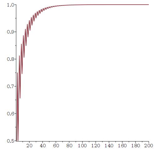
(a) $[[-1,1/2],[2,1/2]]$

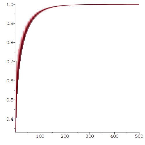
(b) $[[-1,2/3],[3,1/3]]$

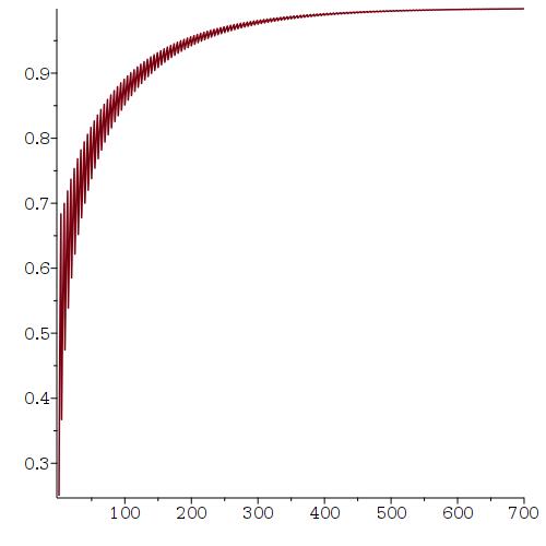
(c) $[[-1,3/4],[4,1/4]]$

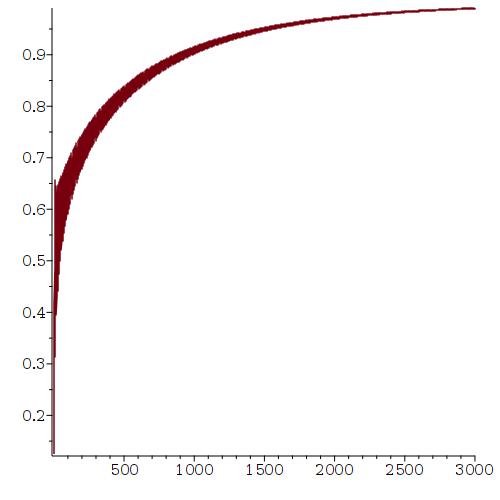
(d) $[[-1,7/8],[8,1/8]]$

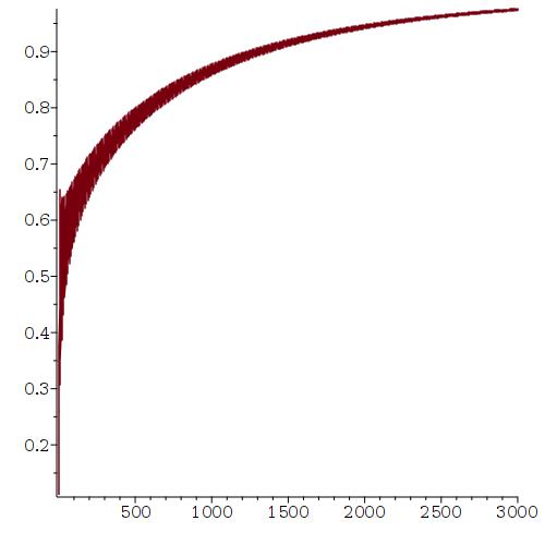
(e) $[[-1,8/9],[9,1/9]]$

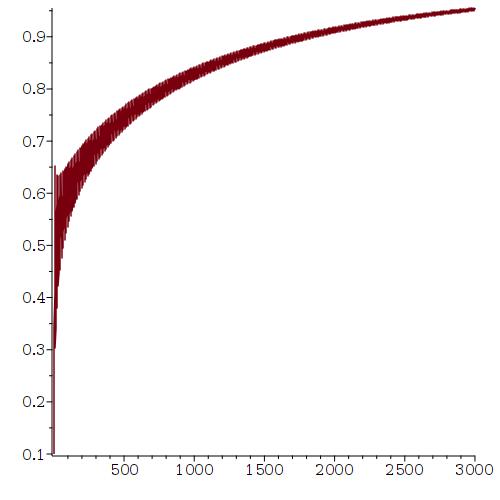
(f) $[[-1,9/10],[10,1/10]]$

Figure 1: The risk-averseness graphs for the corresponding gambles.

The following list describes each of the graphs in figures 2(a), 2(b) and 2(c):

1. The risk-averseness graph for the St. Petersburg Gamble with 7 rounds and entrance fee 7. The graph represents the probability of not losing money if you insist on playing $n$ times, for $n$ from 1 to 300 where the probability table is

   $$[[-5,1/2],[-3,1/4],[1,1/8],[9,1/16],[25,1/32],[57,1/64],[121,1/128],$$

   $$[121,1/128]].$$

2. The approximate risk-averseness graph for the St. Petersburg Gamble with 7 rounds and entrance fee 7, using the Central Limit Theorem Approximation. The graph represents the probability of not losing money if you insist on playing $n$ times, for $n$ from 1 to 2000 where the probability table is the same as in example (a).

3. The approximate risk-averseness graph for the St. Petersburg Gamble with 7 rounds and entrance fee 7, using the Central Limit Theorem Approximation. The graph represents the probability of not losing money if you insist on playing $n$ times, for $n$ from 1 to 2000 where the probability table is

   $$[[-9,1/2],[-7,1/4],[-3,1/8],[5,1/16],[21,1/32],[53,1/64],[117,1/128],$$

   $$[245,1/256],[501,1/512],[1013,1/1024],[2037,1/2048],[2037,1/2048]].$$

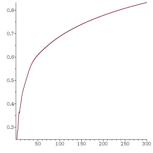
(a)

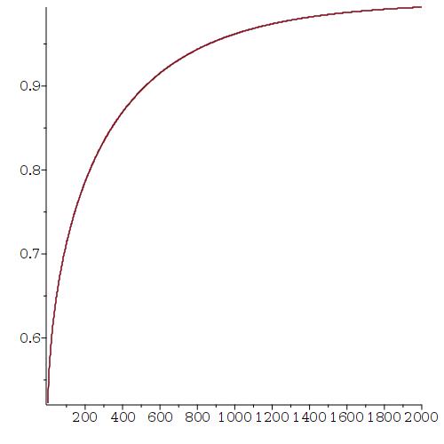
(b)

(c)

Figure 2: The risk-averseness graphs for the corresponding gambles.

 

Lucy Martinez, Department of Mathematics, Rutgers University (New Brunswick), Hill Center-Busch Campus, 110 Frelinghuysen Rd., Piscataway, NJ 08854-8019, USA. Email: lm1154at math dot rutgers dot edu .

Doron Zeilberger, Department of Mathematics, Rutgers University (New Brunswick), Hill Center-Busch Campus, 110 Frelinghuysen Rd., Piscataway, NJ 08854-8019, USA. Email: DoronZeil at gmail dot com .

References

- [1] Almkvist, G., Zeilberger, D. (1990). The method of differentiating under the integral sign. J. Symbolic Computation. 10: 571-591. Available at: https://sites.math.rutgers.edu/~zeilberg/mamarim/mamarimPDF/duis.pdf
- [2] Dougherty-Bliss, R. (2022). Integral Recurrences from A to Z. American Mathematical Monthly. 129: 805-815. Available at: https://arxiv.org/abs/2102.10170
- [3] de Montmort, P. R. (1713). Essay d’analyse sur les jeux de hazard, 2nd ed. Paris, France, pp. 416.