Statistical methods for exoplanet detection with radial velocities

Abstract

Exoplanets can be detected with various observational techniques. Among them, radial velocity (RV) has the key advantages of revealing the architecture of planetary systems and measuring planetary mass and orbital eccentricities. RV observations are poised to play a key role in the detection and characterization of Earth twins. However, the detection of such small planets is not yet possible due to very complex, temporally correlated instrumental and astrophysical stochastic signals. Furthermore, exploring the large parameter space of RV models exhaustively and efficiently presents difficulties. In this review, we frame RV data analysis as a problem of detection and parameter estimation in unevenly sampled, multivariate time series. The objective of this review is two-fold: to introduce the motivation, methodological challenges, and numerical challenges of RV data analysis to nonspecialists, and to unify the existing advanced approaches in order to identify areas for improvement.

1 INTRODUCTION

Until recently, our Solar System was the only laboratory in which to study theories of planetary formation and evolution, and to search for life beyond Earth. The presence of planets outside the Solar system, or exoplanets, was uncertain until the detection of planets orbiting a pulsar (Wolszczan & Frail, 1992). The study of exoplanets as a scientific field accelerated with the detection of 51 Peg b, a planet of minimum $\sim 0.5$ Jupiter mass orbiting a Sun-like star in 4.2 days (Mayor & Queloz, 1995).

The discovery of 51 Peg b, and hundreds of additional exoplanets, was based on the radial velocity method, which is the focus of the present work, and relies on the following principle. A star around which a planet revolves has a periodic reflex motion, so it moves back and forth toward the observer with a certain velocity: its radial velocity (RV). By acquiring spectra of a given star at different times, the observer can measure a time series of RV through the Doppler effect. The amplitude of the variations in RV is proportional to the planetary mass, and its shape depends on the orbital eccentricity.

Mass is one of the most fundamental parameters of a planet. When the radius is measured separately via photometry, the combination of mass and radius gives the density, essential to characterizing the internal structure of the planet, and the surface gravity, key to interpreting measurements of its atmosphere (Kempton et al., 2018, Batalha et al., 2019). The eccentricity is important to understand the formation of planetary systems, especially in multiplanetary systems (e.g. Jurić & Tremaine, 2008).

[] Radial velocity (RV) Velocity of a given star projected onto the direction observer - star. Stellar spectrumNumber of photons collected from a given star per wavelength. Spectrographinstrument used to measure the light flux as a function of its wavelength; can be used to measure the radial velocity of stars

The RV method plays a key role in understanding the demographics of planetary systems, by allowing the detection of planets spanning a much wider range of orbital periods than other detection techniques. Moreover, it does not require a precise orientation of the orbital plane, thereby allowing RVs to characterize planetary systems in which the planets have significant mutual inclinations. As such, RV measurements have a unique potential to reveal the architecture of planetary systems with periods up to $\sim 10$ years (Fulton et al., 2021, Rosenthal et al., 2021)

[] PhotometryNumber of photons collected on a celestial body, here a star, in a broad spectral band as a function of time Transitpassage of a planet between a star and an observer; results in a periodic dip in the flux received

One long-term goal of the scientific community working on exoplanets is to detect and characterize the atmospheres of a population of potentially Earth-like planets, and in particular to search for evidence of life. Characterising the atmosphere of Earth-like planets is beyond the reach of current facilities, but projects of ground based instruments such as PCS@ELT (Kasper et al., 2021), ANDES@ELT, and direct imaging space mission concepts LUVOIR, HaBex or nulling interferometer LIFE (ESA, Quanz et al., 2021)) hope to achieve this by 2050.

Measuring the mass of terrestrial planets to an accuracy of 20% or better is essential to interpreting direct imaging and atmospheric observations (Batalha et al., 2019, Crass et al., 2021). Additionally, detecting Earth-like planets with RV measurements prior to the start of a future direct imaging mission would substantially increase its yield. The RV technique is poised to play a key role in the detection and characterisation of Earth-like planets around Sun-like stars, but we do not yet know if it can achieve the required accuracy. The Earth produces a velocity variation of the Sun of $\mathrm{RV}_{\oplus}$ = 9 cm/s, which we use as a standard unit. The latest-generation of spectrographs (e.g., ESPRESSO (Echelle SPectrograph for Rocky Exoplanets and Stable Spectroscopic Observations), EXPRES (EXtreme PREcision Spectrometer), NEID (NN-EXPLORE Exoplanet Investigations with Doppler spectroscopy)) have demonstrated on-sky precision on a few nights from 3 to 4.5 $\mathrm{RV}_{\oplus}$ (Pepe et al., 2021, Blackman et al., 2020, Lin et al., 2022). If the measurement noise were independent, then 200 measurements would suffice to measure the mass of an Earth-clone with 20% precision, but intrinsic stellar variability causes complex, temporally correlated radial velocity signal of the order of at least 5 $\mathrm{RV}_{\oplus}$. As an example, the RV of the Sun as measured with the HARPS-N spectrograph has a 22 $\mathrm{RV}_{\oplus}$ standard deviation. Characterizing Earth-like planets requires better methods for mitigating stellar variability and instrument systematics. This can be viewed as a particular instance of a general problem: detecting and characterizing periodic signals in multivariate, unevenly sampled time series, corrupted by complex noise.

The present work overviews the efforts undertaken to make Earth twins detectable. The RV data products are presented in §2. We present an overview of the different challenges in §3. We then present RV analysis in a recursive manner: Given summary statistics extracted from raw data and a statistical model of these, the question of how one detects planets and estimates their orbital elements is discussed §4. Given the summary statistics, the question of how one builds a statistical model of the data is treated in §5. How to exploit information in lower data products to extract accurate RVs and useful summary statistics is discussed in §6.

2 DATA AND MODEL

2.1 Doppler shifts

The radial velocity (RV) of a star, its velocity projected onto the line of sight, can be measured due to the Doppler effect. If a source emits a photon with wavelength $\lambda_{0}$, and has a velocity $\mathbf{v}$ relative to an observer, then the wavelength of the photon received is given by

$$\lambda=\lambda_{0}\frac{1+\frac{1}{c}\mathbf{k}\cdot\mathbf{v}}{\sqrt{1-\frac{v^{2}}{c^{2}}}}$$ (1)

where $\cdot$ is the scalar product and $\mathbf{k}$ is the unit vector from the observer to the source (Einstein, 1905). The spectrum of a star contains thousands of absorption lines, short intervals of wavelengths for which photons are absorbed in the upper parts of stellar atmospheres. As the star moves, the Doppler effect causes the apparent wavelength of spectral lines to change (see Fig. 1). An observer who acquires the spectrum of a given star multiple times can measure changes in the apparent wavelength of each spectral line as a function of time, $t$. This maps to measuring $\operatorname{RV}(t)\equiv\mathbf{k}\cdot\mathbf{v}(t)$ in Eq. (1) For more details on the definition of RV, see Lindegren & Dravins (2003) and Lovis & Fischer (2010).

Measuring the radial velocity from a spectrum has many steps, including the correction of instrumental effects. In this review, we start with the estimate of the true stellar spectrum, de-biased from instrumental effects, and transformed to be equivalent to what an observer at the solar system’s center of mass would see. The earlier steps of analysis are briefly presented in Appendix §B.1.

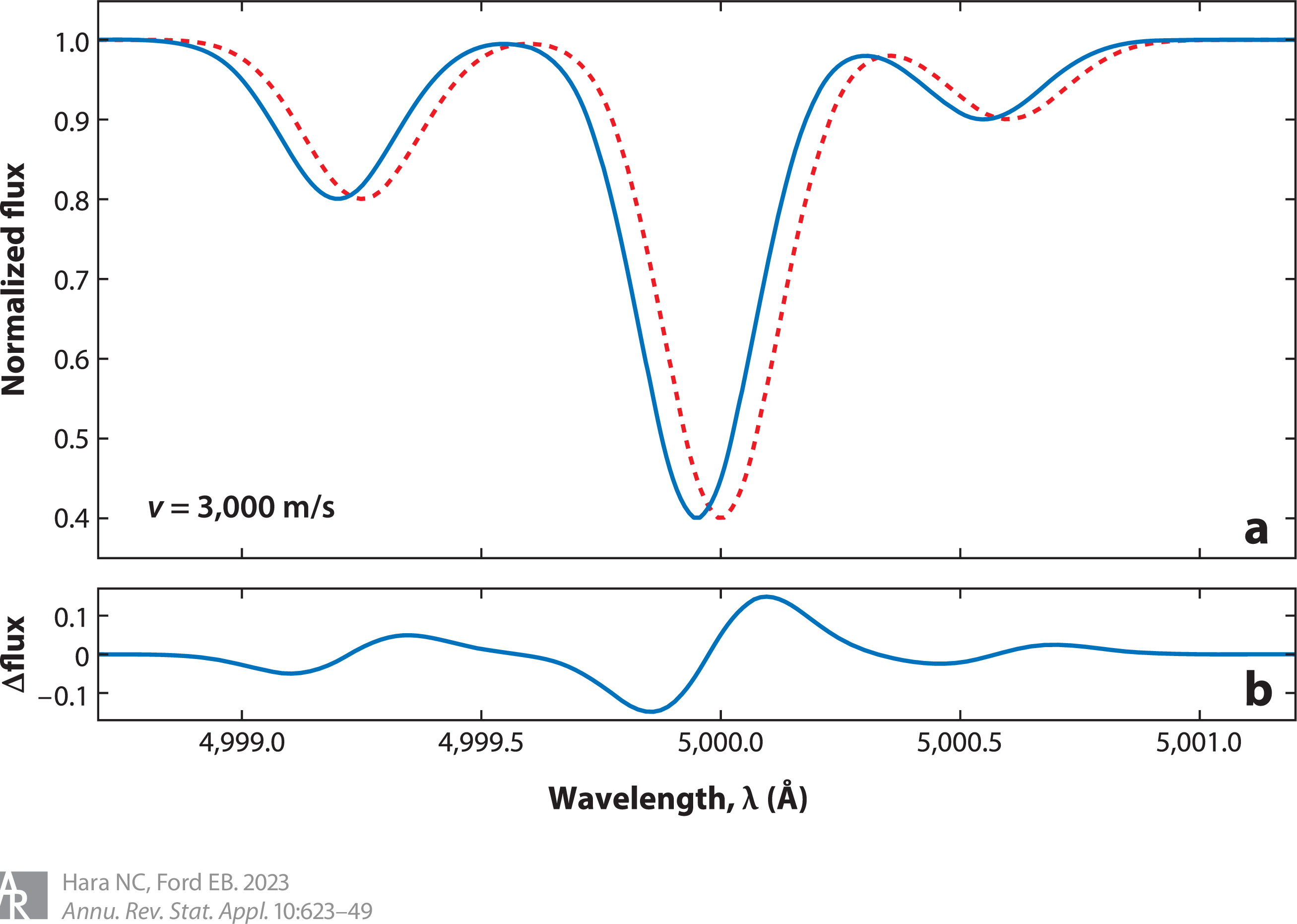
Figure 1: (a) Small portion of a spectrum in rest frame (red, dotted) and in observer frame (blue, solid). (b) Difference in flux between the Doppler-shifted and rest frame spectra. For illustration, we show a large Doppler shift typical of a binary star system. Abbreviation: v, relative velocity of the stars.

2.2 Forward model of planetary effects

An orbiting planet causes a reflex motion of the star, thus creating RV variations. More precisely, the star and the planet periodically traverse elliptical orbits. The star’s RV projected onto the line of sight, or RV, at time $t$ depends on the planet’s mass and orbital parameters and is given by the so-called Keplerian signal,

$$f(t;K,P,e,\omega,M_{0}) = K\left[\cos\left(\omega+\nu(t;e,P,M_{0})\right)+e\cos\omega\right]$$ (2)

where $K,P,e,\omega$, and $M_{0}$ are the velocity amplitude, the orbital period, the orbital eccentricity, the argument of periastron and the mean anomaly describing the motion of the star. The true anomaly, $\nu$, is an angle that parametrizes the position of the star on its orbit (see Appendix §A and Murray & Correia, 2010). Keplerian signalRV signal as a function of time resulting from the orbit of a planet, as given in Eq. 2 and shown in Fig. 2.

The eccentricity of the ellipse is confined to $\left[0,1\right)$ for a bound system undergoing periodic motion. Orbits with $e\simeq~{}0$ are nearly circular and can be well-approximated by the leading terms of a series expansion in the mean anomaly. Orbits with $e\geq~{}0.3$ become obviously elongated and the motion becomes noticeably uneven in time, typically leading to a sharp rise and slow fall (or vice versa), as shown in Fig. 2. Very high eccentricities ($0.9<e<1-R_{\star}/a$, where $R_{\star}$ is the stellar radius and $a$ is the mean star-planet separation) are very rare, but can create numerical difficulties. The signal amplitude depends on the mass of the star and the planet, as well as on the orbital eccentricity, according to the formula

$$K=\left(\frac{2\pi G}{P}\right)^{\frac{1}{3}}\frac{m\sin i}{(m+M)^{\frac{2}{3}}}\frac{1}{\sqrt{1-e^{2}}},$$ (3)

where $M$ is the stellar mass, $m$ is the planet mass, $G$ the gravitational constant, and $i$ is the angle between plane in which the planet orbits and the plane perpendicular to the line of sight (Perryman, 2011). Eq. (3) shows that the RV semi-amplitude is proportional to $m/P^{1/3}$: the more massive the star, and the smaller and farther from its star a planet is, the more difficult the planet is to detect.

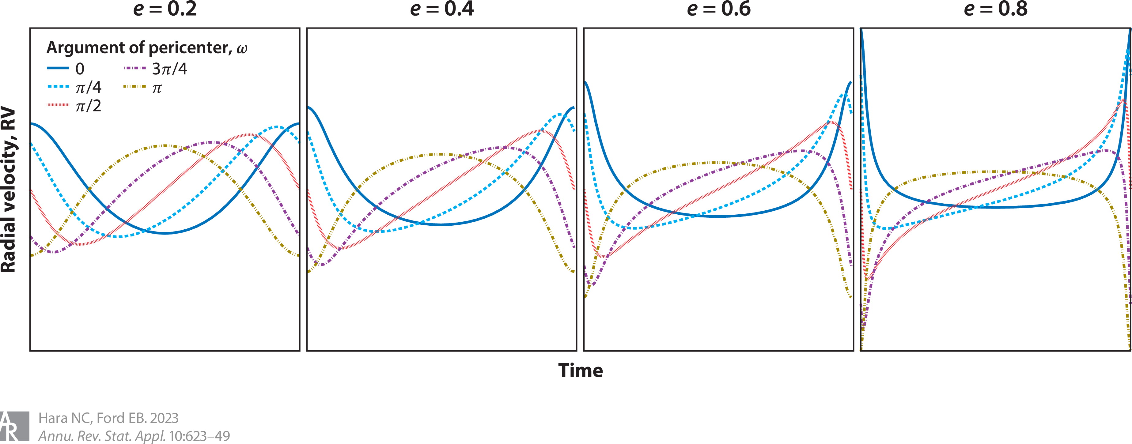
Figure 2: Radial velocity (RV) signature of a single planet. Each panel shows the RV signature over one orbital period for a planet with a given orbital eccentricity e. All curves are computed with the same RV semiamplitude K, and all panels have the same y-axis scale.

Each observed star has a proper motion due to the motion of the star (and the Sun) around the galactic center. On the timescale of RV observations, $\sim 1$ to 20 years, this appears as constant or in some cases a linear trend that must be added to Eq. (2) Furthermore, most Sun-like stars host multiple planets (He et al., 2021). In principle, the planet-planet interactions cause deviations from the Keplerian model, but for the vast majority of planetary systems, the motion of the star can be well-approximated over the timescale of RV surveys as the linear superposition of the Keplerian orbit due to each planet. Hence, our nominal physical model for a time series of RV measurements of a star hosting $n$ planets with parameters $(K_{j},P_{j},e_{j},\omega_{j},{M_{0}}_{j})_{j=1,..,n}$ is

$$\operatorname{RV}(t) = c_{0}+c_{1}t+\sum\limits_{j=1}^{n}f(t;K_{j},P_{j},e_{j},\omega_{j},{M_{0}}_{j}).$$ (4)

The RV amplitude of planet $j$, $K_{j}$ is proportional to $m\sin i$ (see Eq. (3)). In the absence of information on $i$, the planetary mass $m$ cannot be determined unambiguously. Constraints on $i$ can be obtained if the planet transits or, in the case of systems with multiple high-mass short-period planets, due to detecting planet-planet interactions (e.g. Laughlin & Chambers, 2001, Correia et al., 2010, Nelson et al., 2016, Rosenthal et al., 2019).

When the data are acquired with different instruments, it is important to account for the fact that they might have different zero velocity references. Hence, if there are $m$ different instruments, $c_{0}$ in Eq. (4) should be replaced by $\sum_{j=1}^{m}c_{0}^{j}\chi_{j}(t)$, where $\chi_{j}(t)=1$ if the measurement at $t$ is taken by instrument $j$ and 0 otherwise.

2.3 Basic model of observed data

To detect the variations due to planets, astronomers measure the RV of a given star at several irregularly spaced epochs, usually from 20 to 1,000. Each star is only observable when it is high above the horizon, typically for only a few hours per night, and weather can prevent stars from being observed. Furthermore, a star is typically observable for $\sim$ 4-8 months, as it must not be too close to the Sun. Finally, most observatories support multiple science programs, so observations on a given star might be interrupted for a period from hours to weeks.

Each RV measurement has a nominal uncertainty depending on the number of photon received, as well as the properties of star, spectrograph and data reduction technique (Bouchy et al., 2001). Astronomers typically assume independent Gaussian measurement noise at each time $t_{i}$, but in order to reduce the risk of underestimating uncertainties (e.g., unmodeled planets, instrumental noise or stellar variability), an extra Gaussian noise term, often called “jitter”, is added to the model (Ford, 2006), leading to

$$y(t) = \operatorname{RV}(t)+\epsilon(t),$$ (5)

$$\epsilon(t_{i}) \sim N(0,\sigma_{t_{i}}^{2}+\sigma_{J}^{2}),$$ (6)

where $\operatorname{RV}(t)$ is defined in Eq. (4) and the value of the assumed noise for the measurement made at $t_{i}$, $\epsilon(t_{i})$, follows a Gaussian distribution of variance $\sigma_{t_{i}}^{2}+\sigma_{J}^{2}$. Fig. 3 shows an example of a two-planet fit on the RV data of HD114783.

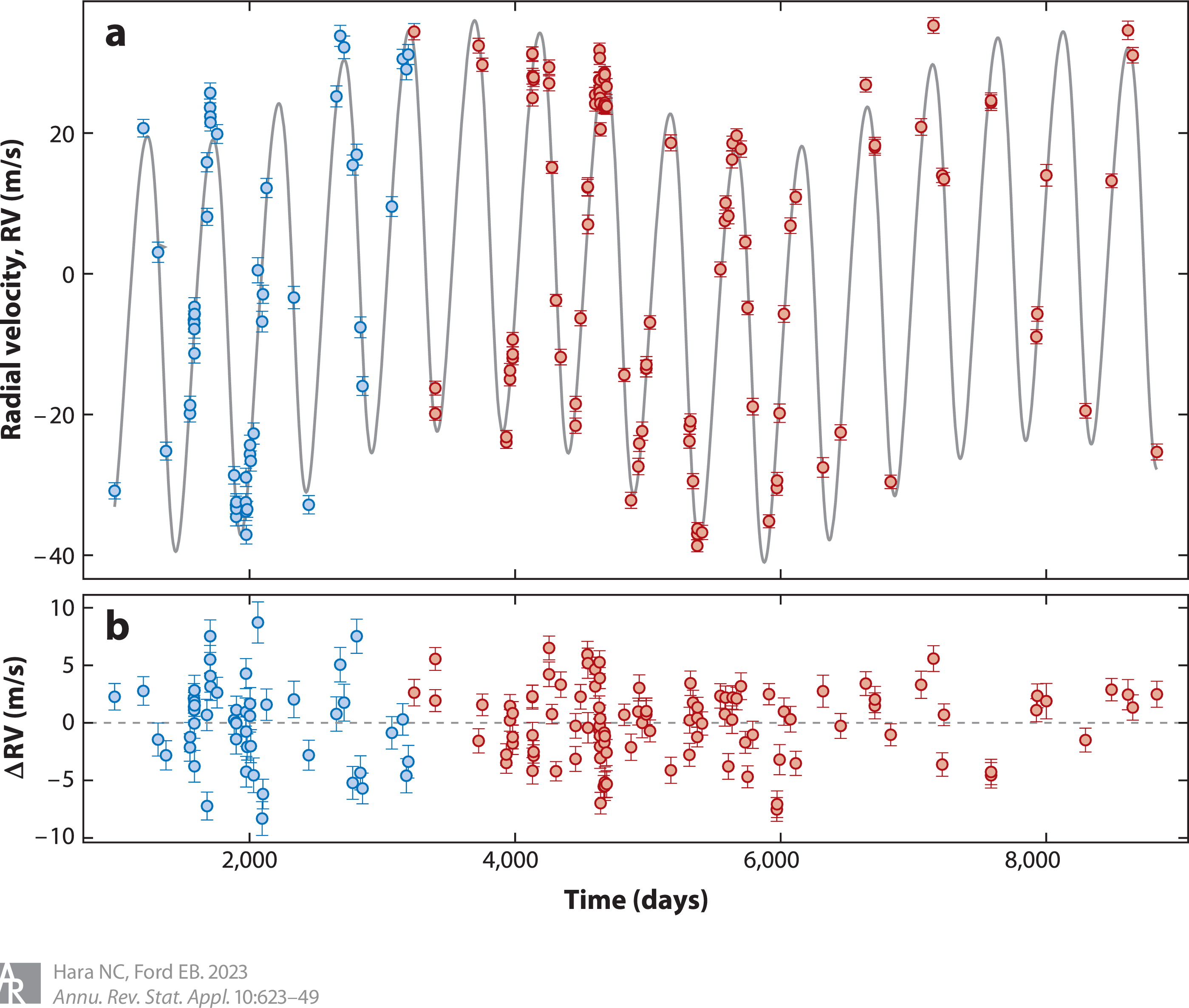
Figure 3: (a) Radial velocity (RV) measurements of the star HD 114783. The gray curve shows the maximum likelihood 2-planet model. (b) RV residuals relative to the 2-planet model above. Error bars reflect reported measurement uncertainties ($\sigma_{t_{i}}$) and do not reflect the 3 m/s of jitter ($\sigma_{J}$). Points are color-coded to indicate whether they are before or after an instrument upgrade that resulted in an unknown RV offset. Data are from Rosenthal et al. (2021).

2.4 Other Processes Affecting RVs

The model in Equations (4)-(6) has been extensively used to estimate the masses and orbital parameters of exoplanets (e.g., Wright & Howard, 2009, Bonomo et al., 2017). For favorable stars, it is useful for analysing RV signals with amplitude over $3-10$ m/s = 33 - 110 $\mathrm{RV}_{\oplus}$, enough to characterise short-period planets with masses greater than Neptune. However, detecting less massive planets requires very precise observations and/or many observations. Accurately interpreting their RV signatures requires greater sophistication because multiple potential noise sources become relevant and require more detailed models for $\epsilon_{t}$. These sources are listed below, and presented in more detail in Appendix B.

2.4.1 Stellar effects

The principle of Doppler spectroscopy is to measure the velocity of a light source with respect to an observer, so if the hot gas in different parts of the stellar surface has different brightness and velocities, it has different impacts on the data. Several physical processes on the surface of stars have an RV signature.

Convection near the surface of the star creates outward and inward motion of the gas. This creates a pattern of evolving convection cells. This process, referred to as granulation, has an effect on RV measurements that can be described as a stationary noise with a Lorentzian or super-Lorentzian power spectrum (Harvey, 1985, Dumusque et al., 2011b, Cegla et al., 2019, Guo et al., 2022). Granulation effects on the RV have been simulated in detail (Meunier et al., 2015, Cegla et al., 2019, Dravins et al., 2021).

Local enhancement of the magnetic field at the surfaces of stars might result in regions darker or brighter than their surroundings, called spots and faculae, respectively (Schrijver, 2002, Strassmeier, 2009). This creates an imbalance in flux from the the approaching and receding side of the rotating star, and reduces upward convection, which has an additional net RV effect. The effect of magnetic activity on RV has been studied in Saar & Donahue (1997), Dumusque et al. (2011a) and Haywood et al. (2016), and simulated in Lagrange et al. (2010), Boisse et al. (2012), Dumusque et al. (2014) and Gilbertson et al. (2020). Active regions grow in size rapidly and disappear more gradually. The visible stellar surface is similar but not identical to itself after one stellar rotation, which results in quasi-periodic RV variations.

The rate of appearance, size and location of spots and faculae varies over a $\sim$ 10 year time-scale on solar-type stars, although it can be down to $\sim$ 1 year for M-type stars (Cortés-Zuleta et al., 2023). This affects the amplitude of short-term RV variations due to magnetic activity (up to 25 m s^-1 (Lovis et al., 2011)) and changes the net RV effect over these timescales. Appendix §B.2 provides a description of known stellar effects affecting RVs, and we refer the reader to Cegla (2019), Meunier (2021), and Crass et al. (2021) for reviews.

2.4.2 Other effects

Residual instrumental systematics and absorption of certain wavelengths by the Earth atmosphere can result in spurious RV signatures of the order of a few $\mathrm{RV}_{\oplus}$ (e.g. Cunha et al., 2014, Artigau et al., 2014, Bertaux et al., 2014, Smette et al., 2015). As they are not amenable to a concise statistical description, we refer the reader to Appendix §B.1 and Halverson et al. (2016), Cretignier et al. (2021) for details.

3 STATISTICAL FRAMEWORK

3.1 Model of RV

The planets only affect the Doppler shift, which must be estimated and converted to RV measurements. We can express the RV extracted from the spectra, $\widehat{\operatorname{RV}(t)}$, as the sum of $\operatorname{RV}(t)$, the RV at time $t$ due to a motion of the center of the mass of the star (in particular due to planets), $\operatorname{RV}_{\mathrm{contam}}(t)$, the RV caused by stellar variability and instrument systematics, and $\epsilon(t)$, the inevitable photon noise. Then, we have

$$\widehat{\operatorname{RV}(t_{i})} =\operatorname{RV}(t_{i})+\operatorname{RV}_{\mathrm{contam}}(t_{i})+\epsilon(t_{i}).$$ (7)

$$\operatorname{RV}(t_{i}) =\operatorname{RV}_{\mathrm{planets}}(t_{i})+\operatorname{RV}_{\mathrm{g}}(t_{i}),i=1,...,N,$$ (8)

where $\operatorname{RV}_{\mathrm{planets}}(t_{i})$ and $\operatorname{RV}_{\mathrm{g}}(t_{i})$ are respectively induced by planets and by other gravitational effects such as companion stars or proper motion in the galaxy. In Eq. (4), $\operatorname{RV}_{g}(t)=c_{0}+c_{1}t$.

In order to interpret RV measurements properly, we must adequately model $\operatorname{RV}_{\mathrm{contam}}(t)$. Unlike planetary RV signals, RV variations induced by the star and instrument do not have a constant frequency, phase, and amplitude (see §4.4), and stellar processes and systematics not only cause a Doppler shift in the spectrum but also cause the shape of the spectrum to vary with time (see Figure 4) and do not affect all lines identically (e. g. Thompson et al., 2017, Wise et al., 2018, Cretignier et al., 2020a, Ning et al., 2019, Wise et al., 2022, Al Moulla et al., 2022a, Lafarga et al., 2023). The shape variations of the spectra can be used to predict the associated $\operatorname{RV}_{\mathrm{contam}}(t)$ signal, either in a machine learning approach with a training set of spectra, or in a statistical framework. In the following section, we show how these ideas can be expressed in a general statistical formalism.

CCF MaskMask: function of the wavelength equal to unity except on wavelength ranges corresponding to spectral lines (see Pepe et al., 2002) Ancillary indicator time series of $N$ scalars extracted from time series of $N$ spectra, summarizing a shape variation of the spectrum, for instance the variations of the average spectral line, or of the amplitude of a specific line.

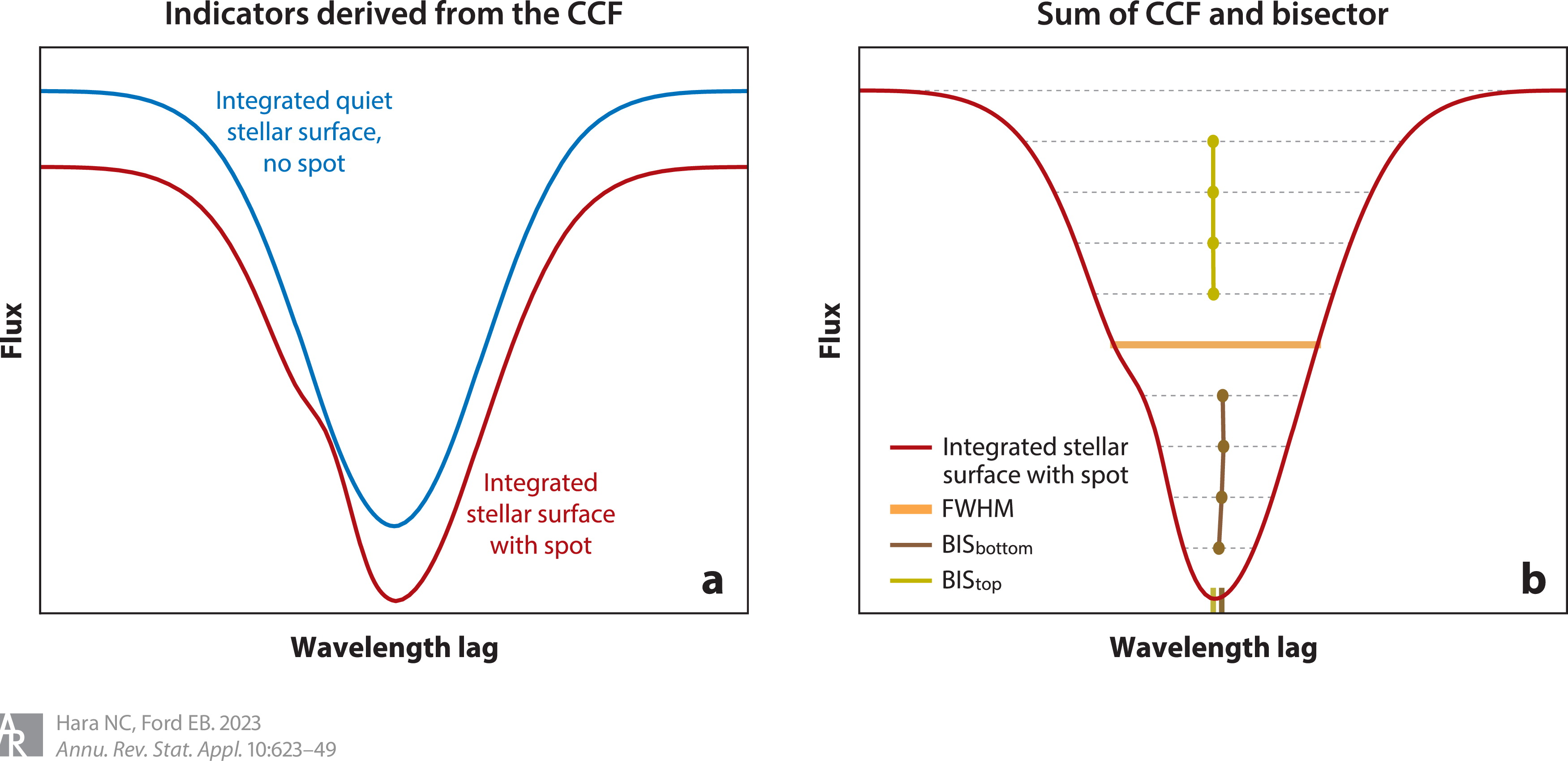
Figure 4: Schematic cross-correlation function (CCF). The scalar product of a mask and the spectrum as a function of the wavelength offset between the two, which can be visualized as an average spectral line. (a) The blue curve shows the CCF of the quiet stellar surface, and the red curve shows the CCF when a dark spot is present on the surface. (b) The CCF when the spot is present has a different full width at half maximum (FWHM) than the CCF of the quiet stellar surface and is asymmetric. The difference between the average position of the lower and upper parts of the CCF, known as bisector inverse slope (BIS) (Queloz et al., 2001), is nonzero. As the star rotates, the spot CCF will have a different Doppler shift: The bump in the red CCF moves from left to right, which also causes the shape of the spectra to change with time, in particular the BIS and FWHM. The spot in this figure covers 20% of the surface, whereas spots on the sun cover $\sim$0.01–0.1% of the surface.

3.2 Challenges of RV data analysis

Our understanding of exoplanets can be thought of as a language where each planet is a word, and each planetary system is a sentence. As in information theory (Shannon, 1948), our knowledge of this language comes through a noisy and biased communication channel. In the long term, we want to understand the full language, but first we must learn to interpret each sentence: what planets orbit a given star? The Bayesian formalism is well suited to describe such situations, and indeed it offers a compact way to present the different problems of RV data analysis (Sandford et al., 2019, also uses an information-theoretic framework for exoplanets).

In our analogy, the message received is the raw data. The most fundamental data product is the number of electrons counted on each CCD detector of the spectrograph. The sentence to be decoded is represented by vectors $\bm{\mathord{\mkern 1.3mu\ThisStyle{\mbox{\hskip 13.76387pt{1 0 -.25 1}\hbox to0.0pt{\hss\leavevmode\hbox{$\SavedStyle\theta$}}}}\mkern-1.3mu}}$ and $\bm{\mathord{\mkern 1.3mu\ThisStyle{\mbox{\hskip 14.03473pt{1 0 -.25 1}\hbox to0.0pt{\hss\leavevmode\hbox{$\SavedStyle\eta$}}}}\mkern-1.3mu}}$. The vector $\bm{\mathord{\mkern 1.3mu\ThisStyle{\mbox{\hskip 13.76387pt{1 0 -.25 1}\hbox to0.0pt{\hss\leavevmode\hbox{$\SavedStyle\theta$}}}}\mkern-1.3mu}}=(\bm{\mathord{\mkern 1.3mu\ThisStyle{\mbox{\hskip 13.76387pt{1 0 -.25 1}\hbox to0.0pt{\hss\leavevmode\hbox{$\SavedStyle\theta$}}}}\mkern-1.3mu}}_{1},...,\bm{\mathord{\mkern 1.3mu\ThisStyle{\mbox{\hskip 13.76387pt{1 0 -.25 1}\hbox to0.0pt{\hss\leavevmode\hbox{$\SavedStyle\theta$}}}}\mkern-1.3mu}}_{n}$) represents the planetary system, where $n$ is the number of planets (which can also be treated as an unknown variable) and $\bm{\mathord{\mkern 1.3mu\ThisStyle{\mbox{\hskip 13.76387pt{1 0 -.25 1}\hbox to0.0pt{\hss\leavevmode\hbox{$\SavedStyle\theta$}}}}\mkern-1.3mu}}_{j}$ the orbital elements of planet indexed by $j$ (see Eq. (2)). The vector $\bm{\mathord{\mkern 1.3mu\ThisStyle{\mbox{\hskip 14.03473pt{1 0 -.25 1}\hbox to0.0pt{\hss\leavevmode\hbox{$\SavedStyle\eta$}}}}\mkern-1.3mu}}$ includes all other relevant non-planetary parameters, such as an offset, a drift, the stellar rotation period, noise amplitude and timescale.

Let us denote the lowest-level data by $\mathbf{D}$. Our goal is to obtain a meaningful joint posterior distribution for $\bm{\mathord{\mkern 1.3mu\ThisStyle{\mbox{\hskip 14.03473pt{1 0 -.25 1}\hbox to0.0pt{\hss\leavevmode\hbox{$\SavedStyle\eta$}}}}\mkern-1.3mu}}$ and $\bm{\mathord{\mkern 1.3mu\ThisStyle{\mbox{\hskip 13.76387pt{1 0 -.25 1}\hbox to0.0pt{\hss\leavevmode\hbox{$\SavedStyle\theta$}}}}\mkern-1.3mu}}$ knowing $\mathbf{D}$, $p(\bm{\mathord{\mkern 1.3mu\ThisStyle{\mbox{\hskip 13.76387pt{1 0 -.25 1}\hbox to0.0pt{\hss\leavevmode\hbox{$\SavedStyle\theta$}}}}\mkern-1.3mu}},\bm{\mathord{\mkern 1.3mu\ThisStyle{\mbox{\hskip 14.03473pt{1 0 -.25 1}\hbox to0.0pt{\hss\leavevmode\hbox{$\SavedStyle\eta$}}}}\mkern-1.3mu}}\mid\mathbf{D})$, but $\mathbf{D}$ is corrupted by hundreds of instrumental effects, and computing the posterior directly is currently unmanageable. To be usable $\mathbf{D}$ needs to be reduced to an estimate of the RV time series $\mathbf{\widehat{\operatorname{RV}}}=(\widehat{\operatorname{RV}}(t_{i}))_{i=1,..,N}$ and ancillary indicators $\mathbf{I}=(\mathbf{I}_{j}(t_{i}))_{j=1..p,i=1..N}$, such that for each $j$, $\mathbf{I}_{j}(\mathbf{t})$ is a time series of length $N$, summarizing the variations of shape of the spectrum (see Fig. 4.b). With notations of Eqs. (7) and (8),

$$p(\bm{\mathord{\mkern 1.3mu\ThisStyle{\mbox{\hskip 13.76387pt{1 0 -.25 1}\hbox to0.0pt{\hss\leavevmode\hbox{$\SavedStyle\theta$}}}}\mkern-1.3mu}},\bm{\mathord{\mkern 1.3mu\ThisStyle{\mbox{\hskip 14.03473pt{1 0 -.25 1}\hbox to0.0pt{\hss\leavevmode\hbox{$\SavedStyle\eta$}}}}\mkern-1.3mu}}\mid\mathbf{D})\approx p(\bm{\mathord{\mkern 1.3mu\ThisStyle{\mbox{\hskip 13.76387pt{1 0 -.25 1}\hbox to0.0pt{\hss\leavevmode\hbox{$\SavedStyle\theta$}}}}\mkern-1.3mu}},\bm{\mathord{\mkern 1.3mu\ThisStyle{\mbox{\hskip 14.03473pt{1 0 -.25 1}\hbox to0.0pt{\hss\leavevmode\hbox{$\SavedStyle\eta$}}}}\mkern-1.3mu}}\mid\mathbf{I},\widehat{\mathbf{RV}}) =\frac{p(\mathbf{I},\widehat{\mathbf{RV}}\mid\bm{\mathord{\mkern 1.3mu\ThisStyle{\mbox{\hskip 13.76387pt{1 0 -.25 1}\hbox to0.0pt{\hss\leavevmode\hbox{$\SavedStyle\theta$}}}}\mkern-1.3mu}},\bm{\mathord{\mkern 1.3mu\ThisStyle{\mbox{\hskip 14.03473pt{1 0 -.25 1}\hbox to0.0pt{\hss\leavevmode\hbox{$\SavedStyle\eta$}}}}\mkern-1.3mu}})p(\bm{\mathord{\mkern 1.3mu\ThisStyle{\mbox{\hskip 13.76387pt{1 0 -.25 1}\hbox to0.0pt{\hss\leavevmode\hbox{$\SavedStyle\theta$}}}}\mkern-1.3mu}},\bm{\mathord{\mkern 1.3mu\ThisStyle{\mbox{\hskip 14.03473pt{1 0 -.25 1}\hbox to0.0pt{\hss\leavevmode\hbox{$\SavedStyle\eta$}}}}\mkern-1.3mu}})}{p(\mathbf{I},\widehat{\mathbf{RV}})}=\frac{p(\mathbf{I},\mathbf{RV}_{\mathrm{contam}}+\bm{\mathord{\mkern 1.3mu\ThisStyle{\mbox{\hskip 13.12846pt{1 0 -.25 1}\hbox to0.0pt{\hss\leavevmode\hbox{$\SavedStyle\epsilon$}}}}\mkern-1.3mu}}\mid\bm{\mathord{\mkern 1.3mu\ThisStyle{\mbox{\hskip 13.76387pt{1 0 -.25 1}\hbox to0.0pt{\hss\leavevmode\hbox{$\SavedStyle\theta$}}}}\mkern-1.3mu}},\bm{\mathord{\mkern 1.3mu\ThisStyle{\mbox{\hskip 14.03473pt{1 0 -.25 1}\hbox to0.0pt{\hss\leavevmode\hbox{$\SavedStyle\eta$}}}}\mkern-1.3mu}})p(\bm{\mathord{\mkern 1.3mu\ThisStyle{\mbox{\hskip 13.76387pt{1 0 -.25 1}\hbox to0.0pt{\hss\leavevmode\hbox{$\SavedStyle\theta$}}}}\mkern-1.3mu}},\bm{\mathord{\mkern 1.3mu\ThisStyle{\mbox{\hskip 14.03473pt{1 0 -.25 1}\hbox to0.0pt{\hss\leavevmode\hbox{$\SavedStyle\eta$}}}}\mkern-1.3mu}})}{p(\mathbf{I},\widehat{\mathbf{RV}})}.$$ (9)

The last equality comes from the fact that $\operatorname{RV}(t)$ depends deterministically on $\bm{\mathord{\mkern 1.3mu\ThisStyle{\mbox{\hskip 13.76387pt{1 0 -.25 1}\hbox to0.0pt{\hss\leavevmode\hbox{$\SavedStyle\theta$}}}}\mkern-1.3mu}},\bm{\mathord{\mkern 1.3mu\ThisStyle{\mbox{\hskip 14.03473pt{1 0 -.25 1}\hbox to0.0pt{\hss\leavevmode\hbox{$\SavedStyle\eta$}}}}\mkern-1.3mu}}$. Below, we denote $\mathbf{y}=(\widehat{\mathbf{RV}},\mathbf{I})$, potentially with $\mathbf{I}=\emptyset$. We will refer to $p(\bm{\mathord{\mkern 1.3mu\ThisStyle{\mbox{\hskip 13.76387pt{1 0 -.25 1}\hbox to0.0pt{\hss\leavevmode\hbox{$\SavedStyle\theta$}}}}\mkern-1.3mu}},\bm{\mathord{\mkern 1.3mu\ThisStyle{\mbox{\hskip 14.03473pt{1 0 -.25 1}\hbox to0.0pt{\hss\leavevmode\hbox{$\SavedStyle\eta$}}}}\mkern-1.3mu}})$ as the prior distribution and $p(\mathbf{y}\mid\bm{\mathord{\mkern 1.3mu\ThisStyle{\mbox{\hskip 13.76387pt{1 0 -.25 1}\hbox to0.0pt{\hss\leavevmode\hbox{$\SavedStyle\theta$}}}}\mkern-1.3mu}},\bm{\mathord{\mkern 1.3mu\ThisStyle{\mbox{\hskip 14.03473pt{1 0 -.25 1}\hbox to0.0pt{\hss\leavevmode\hbox{$\SavedStyle\eta$}}}}\mkern-1.3mu}})$ as the likelihood. In some cases, to emphasize that the likelihood is restricted to models with exactly $n$ planets we will denote the likelihood by $p(\mathbf{y}\mid\bm{\mathord{\mkern 1.3mu\ThisStyle{\mbox{\hskip 13.76387pt{1 0 -.25 1}\hbox to0.0pt{\hss\leavevmode\hbox{$\SavedStyle\theta$}}}}\mkern-1.3mu}},\bm{\mathord{\mkern 1.3mu\ThisStyle{\mbox{\hskip 14.03473pt{1 0 -.25 1}\hbox to0.0pt{\hss\leavevmode\hbox{$\SavedStyle\eta$}}}}\mkern-1.3mu}},n)$. This formalism also accounts for the case where photometric data of the target star is also available: the photometry time series can be considered as another indicator, with the added complexity that the data is not acquired at the same epochs as the spectra. Reduced datavector y concatenating the RV time series and ancillary indicators, extracted from the raw data $\mathbf{D}$

Likelihoodprobability distribution of the reduced data $\mathbf{y}$ knowing the model parameters $\bm{\mathord{\mkern 1.3mu\ThisStyle{\mbox{\hskip 13.76387pt{1 0 -.25 1}\hbox to0.0pt{\hss\leavevmode\hbox{$\SavedStyle\theta$}}}}\mkern-1.3mu}}$ and $\bm{\mathord{\mkern 1.3mu\ThisStyle{\mbox{\hskip 14.03473pt{1 0 -.25 1}\hbox to0.0pt{\hss\leavevmode\hbox{$\SavedStyle\eta$}}}}\mkern-1.3mu}}$; denoted by $p(\mathbf{y}\mid\bm{\mathord{\mkern 1.3mu\ThisStyle{\mbox{\hskip 13.76387pt{1 0 -.25 1}\hbox to0.0pt{\hss\leavevmode\hbox{$\SavedStyle\theta$}}}}\mkern-1.3mu}},\bm{\mathord{\mkern 1.3mu\ThisStyle{\mbox{\hskip 14.03473pt{1 0 -.25 1}\hbox to0.0pt{\hss\leavevmode\hbox{$\SavedStyle\eta$}}}}\mkern-1.3mu}})$

Based on Eq. 9, we can identify several choices to be made: $(a)$ a reduction method transforming the observational raw data into summary statistics $\widehat{\mathbf{RV}},\mathbf{I}$ that estimate the RV and provide useful indicators of spectral variability; $(b)$ a model, that is a likelihood $p(\mathbf{y}\mid\bm{\mathord{\mkern 1.3mu\ThisStyle{\mbox{\hskip 13.76387pt{1 0 -.25 1}\hbox to0.0pt{\hss\leavevmode\hbox{$\SavedStyle\theta$}}}}\mkern-1.3mu}},\bm{\mathord{\mkern 1.3mu\ThisStyle{\mbox{\hskip 14.03473pt{1 0 -.25 1}\hbox to0.0pt{\hss\leavevmode\hbox{$\SavedStyle\eta$}}}}\mkern-1.3mu}})$ and prior distribution $p(\bm{\mathord{\mkern 1.3mu\ThisStyle{\mbox{\hskip 13.76387pt{1 0 -.25 1}\hbox to0.0pt{\hss\leavevmode\hbox{$\SavedStyle\theta$}}}}\mkern-1.3mu}},\bm{\mathord{\mkern 1.3mu\ThisStyle{\mbox{\hskip 14.03473pt{1 0 -.25 1}\hbox to0.0pt{\hss\leavevmode\hbox{$\SavedStyle\eta$}}}}\mkern-1.3mu}})$. The key difference with step $(a)$ is that the effect of potential planets is now explicitly included in the likelihood definition; $(c)$ a decision method for confidently claiming the detection of planetary signals and estimating their masses and orbital elements for a given model, or a collection of models. In the Bayesian formalism above, the decision is based on the posterior distribution $p(\bm{\mathord{\mkern 1.3mu\ThisStyle{\mbox{\hskip 13.76387pt{1 0 -.25 1}\hbox to0.0pt{\hss\leavevmode\hbox{$\SavedStyle\theta$}}}}\mkern-1.3mu}},\bm{\mathord{\mkern 1.3mu\ThisStyle{\mbox{\hskip 14.03473pt{1 0 -.25 1}\hbox to0.0pt{\hss\leavevmode\hbox{$\SavedStyle\eta$}}}}\mkern-1.3mu}}\mid\mathbf{y})$ and must include a discussion of its sensitivity of the result to the choices made in $a$ and $b$. The Bayesian formalism only serves here to compactly present points $a$–$c$ and is not always used in practice. Points $a$, $b$, and $c$ are treated recursively in §6, 5 and 4, respectively, and must be completed by $(d)$ a set of practical and reliable numerical methods for performing the necessary calculations. Numerical aspects are highlighted when relevant.

4 DETECTING PLANETS AND ESTIMATING THEIR ORBITAL ELEMENTS

4.1 Likelihood

Suppose that we have at our disposal an RV time series, a few ancillary indicators and a statistical model of them. We want to determine how many planets can be confidently detected, and what their orbital elements are.

In §3, we presented the different steps of exoplanet detection, and in particular of a likelihood function describing the distribution of data $\mathbf{y}$ as a function of the model parameters $\bm{\mathord{\mkern 1.3mu\ThisStyle{\mbox{\hskip 13.76387pt{1 0 -.25 1}\hbox to0.0pt{\hss\leavevmode\hbox{$\SavedStyle\theta$}}}}\mkern-1.3mu}}$ and $\bm{\mathord{\mkern 1.3mu\ThisStyle{\mbox{\hskip 14.03473pt{1 0 -.25 1}\hbox to0.0pt{\hss\leavevmode\hbox{$\SavedStyle\eta$}}}}\mkern-1.3mu}}$, describing respectively the planets and all other effects. The likelihood is commonly assumed to be Gaussian,

$$\mathcal{L}\equiv p(\mathbf{y}\mid\bm{\mathord{\mkern 1.3mu\ThisStyle{\mbox{\hskip 13.76387pt{1 0 -.25 1}\hbox to0.0pt{\hss\leavevmode\hbox{$\SavedStyle\theta$}}}}\mkern-1.3mu}},\bm{\mathord{\mkern 1.3mu\ThisStyle{\mbox{\hskip 14.03473pt{1 0 -.25 1}\hbox to0.0pt{\hss\leavevmode\hbox{$\SavedStyle\eta$}}}}\mkern-1.3mu}})=\frac{\operatorname{e}^{-\frac{1}{2}\left[\mathbf{y}-\mathbf{g}(\mathbf{t};\bm{\mathord{\mkern 1.3mu\ThisStyle{\mbox{\hskip 9.6347pt{1 0 -.25 1}\hbox to0.0pt{\hss\leavevmode\hbox{$\SavedStyle\theta$}}}}\mkern-1.3mu}},\bm{\mathord{\mkern 1.3mu\ThisStyle{\mbox{\hskip 9.82431pt{1 0 -.25 1}\hbox to0.0pt{\hss\leavevmode\hbox{$\SavedStyle\eta$}}}}\mkern-1.3mu}})\right]^{T}\mathbf{V(\bm{\mathord{\mkern 1.3mu\ThisStyle{\mbox{\hskip 9.82431pt{1 0 -.25 1}\hbox to0.0pt{\hss\leavevmode\hbox{$\SavedStyle\eta$}}}}\mkern-1.3mu}})}^{-1}\left[\mathbf{y}-\mathbf{g}(\mathbf{t};\bm{\mathord{\mkern 1.3mu\ThisStyle{\mbox{\hskip 9.6347pt{1 0 -.25 1}\hbox to0.0pt{\hss\leavevmode\hbox{$\SavedStyle\theta$}}}}\mkern-1.3mu}},\bm{\mathord{\mkern 1.3mu\ThisStyle{\mbox{\hskip 9.82431pt{1 0 -.25 1}\hbox to0.0pt{\hss\leavevmode\hbox{$\SavedStyle\eta$}}}}\mkern-1.3mu}})\right]}}{\sqrt{(2\pi)^{N}|\mathbf{V}(\bm{\mathord{\mkern 1.3mu\ThisStyle{\mbox{\hskip 14.03473pt{1 0 -.25 1}\hbox to0.0pt{\hss\leavevmode\hbox{$\SavedStyle\eta$}}}}\mkern-1.3mu}})|}}.$$ (10)

where $|\mathbf{V}(\bm{\mathord{\mkern 1.3mu\ThisStyle{\mbox{\hskip 14.03473pt{1 0 -.25 1}\hbox to0.0pt{\hss\leavevmode\hbox{$\SavedStyle\eta$}}}}\mkern-1.3mu}})|$ is the determinant of the covariance matrix $\mathbf{V}(\bm{\mathord{\mkern 1.3mu\ThisStyle{\mbox{\hskip 14.03473pt{1 0 -.25 1}\hbox to0.0pt{\hss\leavevmode\hbox{$\SavedStyle\eta$}}}}\mkern-1.3mu}})$. For instance, supposing that $\mathbf{y}$ is the RV time series, using model (4)-(6), $\bm{\mathord{\mkern 1.3mu\ThisStyle{\mbox{\hskip 13.76387pt{1 0 -.25 1}\hbox to0.0pt{\hss\leavevmode\hbox{$\SavedStyle\theta$}}}}\mkern-1.3mu}}=(K_{j},P_{j},e_{j},\omega_{j},{M_{0}}_{j})_{j=1,..,{n}}$, $\mathbf{g}$ is the sum of Keplerians and an affine function (see Eq. (4)), and $\bm{\mathord{\mkern 1.3mu\ThisStyle{\mbox{\hskip 14.03473pt{1 0 -.25 1}\hbox to0.0pt{\hss\leavevmode\hbox{$\SavedStyle\eta$}}}}\mkern-1.3mu}}=\sigma_{J},c_{0},c_{1}$, $\mathbf{V}$ is diagonal with $i$-th element $\sigma_{t_{i}}^{2}+\sigma_{J}^{2}$. If $\operatorname{RV}_{\mathrm{contam}}$ is non-zero, it might be modelled by a non-diagonal matrix $\mathbf{V}(\bm{\mathord{\mkern 1.3mu\ThisStyle{\mbox{\hskip 14.03473pt{1 0 -.25 1}\hbox to0.0pt{\hss\leavevmode\hbox{$\SavedStyle\eta$}}}}\mkern-1.3mu}})$, and/or a linear model of stellar activity indicators in $\mathbf{g}$. This form of the likelihood is used both when the data $\mathbf{y}$ is the RV time series only, a single ancillary indicator, or the concatenation of the time series of RV and ancillary indicators (possibly including also photometric observations of the target star). We return to how to specify further $\mathbf{g}(\mathbf{t};\bm{\mathord{\mkern 1.3mu\ThisStyle{\mbox{\hskip 13.76387pt{1 0 -.25 1}\hbox to0.0pt{\hss\leavevmode\hbox{$\SavedStyle\theta$}}}}\mkern-1.3mu}})$ and $\mathbf{V}(\bm{\mathord{\mkern 1.3mu\ThisStyle{\mbox{\hskip 14.03473pt{1 0 -.25 1}\hbox to0.0pt{\hss\leavevmode\hbox{$\SavedStyle\eta$}}}}\mkern-1.3mu}})$ in §5.

Assessing the statistical significance of a putative RV signal is remarkably challenging. We review three broad approaches: periodogram-based methods (§4.2.2), Bayesian model comparison (§4.3), and in §4.4, we present approaches that do not aim to specify an explicit model for nuisance signals, but aim to obtain robust detections.

4.2 Planet Detection via Periodograms

The decision on the planets detected and their orbital elements should make use of the full posterior of orbital elements, or in a frequentist setting the full likelihood. However, computing the posterior distribution of elements given in Eq. (9) or exploring exhaustively the parameter space to evaluate the likelihood is only possible with the latest numerical tools, and is computationally intensive. Realistic datasets often have millions of local likelihood maxima. Historically, the exploration of likelihood modes was done with periodogram methods, which are still extensively used due to their speed, numerical stability, and ability to unveil the dominating frequencies in the data.

4.2.1 Definition

Given a time series, for instance the RV time series, or the time series of a given ancillary indicator, periodograms consist in comparing the log-likelihoods of two models: a base model $H_{0}$ and a model $K_{\omega}$ including $H_{0}$ plus a periodic component at fre- quency $\omega$, for a grid of frequencies. In periodograms, the Keplerian model is often replaced with an approximation that yields a convex model once conditioned on a small number of parameters.

The first and simplest case is the Lomb–Scargle periodogram (Lomb, 1976, Scargle, 1982), where the base model $H_{0}$ is Gaussian white noise, and $K_{\omega}$ is the same white noise plus a sine function. Both $H_{0}$ and $K_{\omega}$ are described with likelihoods such as that (10), with

$$H_{0}:\; \mathbf{g}=\mathbf{0},$$ (11)

$$K_{\omega}:\; \mathbf{g}(A,B,\omega)=A\cos\omega\mathbf{t}+B\sin\omega\mathbf{t},$$ (12)

and $\mathbf{V}=\mathrm{diag}((\sigma_{i}^{2})_{i=1,...,N})$ in both models. In $K_{\omega}$, $\mathbf{g}$ is the exact RV signature of a planet on a circular orbit ($e=0$) with orbital period $P=2\pi/\omega$ and is a good approximation when $eK\leq\sigma_{\mathrm{RV,ideal}}$. For a given $\omega$, maximizing the likelihood with respect to $A$ and $B$ is equivalent to to minimizing the sum of squares, and it is a linear problem. The Lomb–Scargle periodogram is then the difference of the log-likelihoods of models $H_{0}$ and $K_{\omega}$ as a function of $\omega$.

The principle of the periodogram can be extended with more complex definitions of $H_{0}$ and $K_{\omega}$ and/or by interpreting the periodogram in a Bayesian context. The null hypothesis $H_{0}$ can be complexified (e. g. Baluev, 2008), the periodic signals might be chosen as nonsinusoidal (e. g. Baluev, 2013a, 2015b), and the assumption that the noise is uncorrelated can be dropped (e.g. Delisle et al., 2020a). Figure 5 shows an example of the application of different types of periodograms. A comprehensive list of existing periodograms is given in Appendix C.

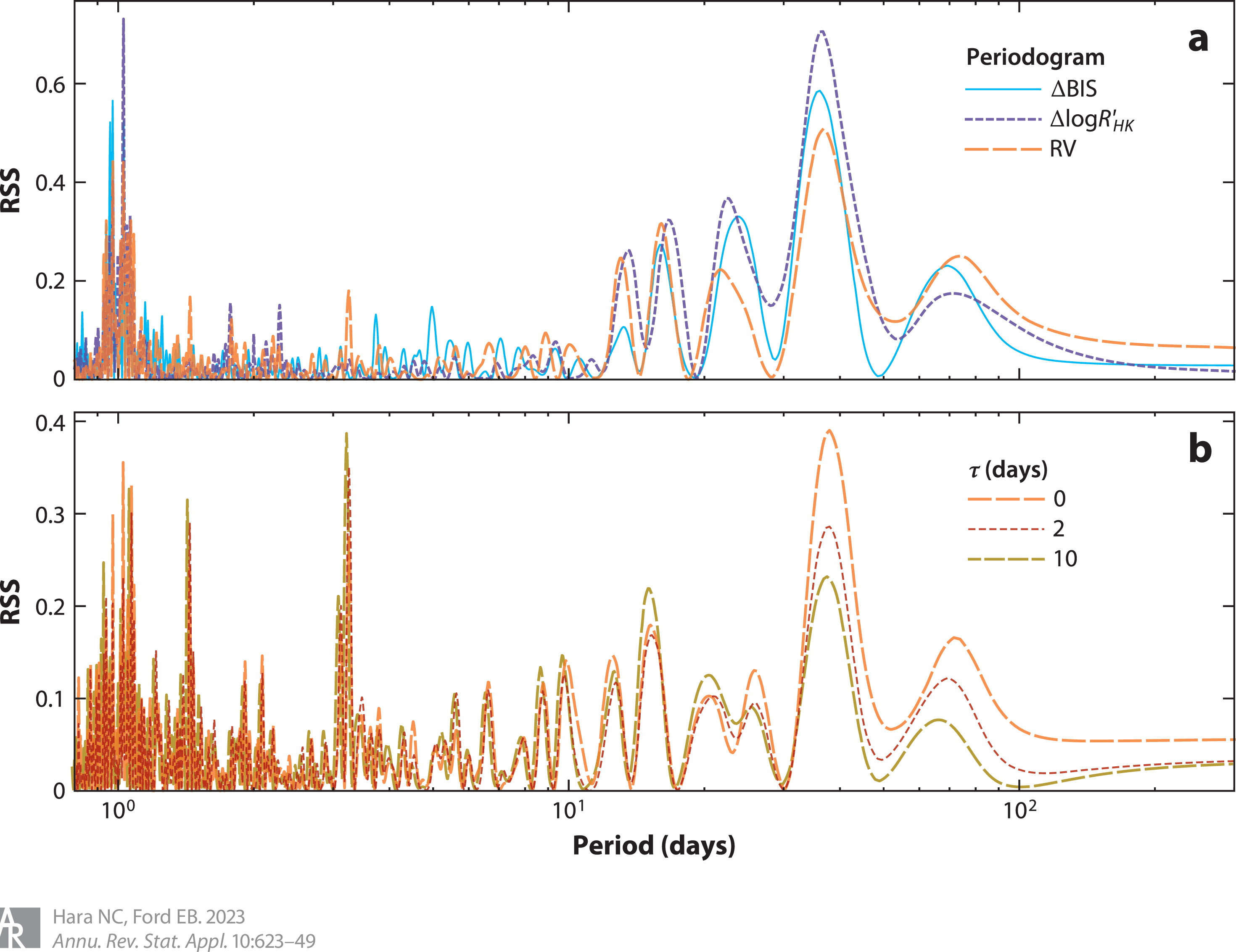
Figure 5: (a) generalized Lomb–Scargle periodograms of the time series of two ancillary indicators: bisector inverse slope, $\Delta$BIS (Queloz et al., 2001), and $\Delta\log R^{\prime}_{HK}$ (Noyes, 1984)), and RV time series (RV) of the ESPRESSO (Echelle SPectrograph for Rocky Exoplanets and Stable Spectroscopic Observations) data of the star TOI 178178 (Leleu et al., 2021). The time series of $\Delta$BIS, $\log R^{\prime}_{HK}$ and RV are shown in Fig. 7. Periodograms are expressed in reduction in sum of squares (RSS), normalized — that is, the difference between residual sum of squares after fitting $H_{0}$ and $K_{\omega}$, divided by that of the $H_{0}$ residuals (see Eqs. (11) and (12)). The periodogram presents peaks around a period of 1 day, due to the repetition of observations every 24 hours $\pm$ 2-3 h (Dawson & Fabrycky, 2010). All three time series present power at $\sim 40$ days, due to stellar rotation. (b) In orange, periodogram of the RV time series when the $\Delta\log R^{\prime}_{HK}$ and $\Delta$BIS are included as a linear predictors in the $H_{0}$ and $K_{\omega}$ models. This damps the amplitude of the stellar rotation: / signal, and a peak at 3.2 days emerges. The red and light brown curves correspond to adding a correlated noise Gaussian model in the covariance with a Gaussian kernel of amplitude 1 m/s and timescale 2 or 10 days. Adding correlated noise models always damps power at low frequencies (for details, see Delisle et al. (2020a)).

4.2.2 Periodogram-based model comparison

The usual way to determine whether a periodogram supports the detection of a periodic signal is to compute $p(\max_{\omega}\mathcal{P}(\omega)\mid H_{0})$ the probability distribution of the maximum value of the periodogram, $\max_{\omega}\mathcal{P}(\omega)$ under a null hypothesis, $H_{0}$. We compute the maximum of the periodogram for the data to be analyzed, $\mathcal{P}_{\mathrm{d}}$ on a grid of frequencies $\Omega=(\omega_{i})_{i=1..N}$, and define a false alarm probability, FAP, as $p(\max_{\omega\in\Omega}\mathcal{P}(\omega)\geqslant\mathcal{P}_{\mathrm{d}}\mid H_{0})$.

The FAP is most robustly estimated by generating signals under the null hypothesis, and the FAP estimated is the fraction of simulations with a maximum peak greater than $\mathcal{P}_{\mathrm{d}}$. This is computationally expensive, as it requires $\sim n$ simulations for a precision of $100/n\%$ on the FAP. Since astronomers often aim for a FAP of $<$ 0.1% to 0.01%, $n>10^{4}$ is needed.

A semianalytical approach allows one to simulate a reduced number of signals and to fit a generalised extreme value distribution (Süveges, 2014) to the empirical distribution. The analytical approach approximates the FAP thanks to the theory of extreme values of stochastic processes using the Rice formula (Baluev, 2008, 2009, 2013), even for complex periodic shapes (Baluev, 2013a, 2015b) or correlated noise (Delisle et al., 2020a). These analytical approximations are very accurate in practice if at least a few tens of data points are available (Süveges et al., 2015).

4.2.3 Pros and cons

Periodograms are fast and numerically stable, and the advent of accurate analytical estimates of the FAP, even in the case where signals are searched for simultaneously (Baluev, 2013) or with Gaussian correlated noise models (Delisle et al., 2020a), further simplifies their use. They provide a useful visual diagnostic of the frequency content of the signal. However, they have drawbacks.

First, most periodograms scan for the orbital period of one planet at a time. For multiple planet systems, periodograms can be applied iteratively, first to identify the most conspicuous planet from the data, then to look for a $(j+1)$th planet in the residuals of the best-fit model using $j$ planets. However, periodograms are sensitive to aliasing, or spectral leakage, (Dawson & Fabrycky, 2010). Aliases of different signals can add destructively or coherently, so, even if the highest peak of a periodogram is statistically significant, its period may not match that of any physical signal. This can be avoided by searching for multiple signals simultaneously (Ford et al., 2011, Baluev, 2013). Brute force search for two signals at once is expensive and allowing for more rapidly becomes prohibitive. Other approaches based on sparse recovery allow one to search for several signals at low computational cost (Hara et al., 2017).

Stellar activity causes low-frequency signals which can be mistaken for planets. It is better not only to search for several planets simultaneously but also to fit the parameters of stellar activity and planetary signals jointly. As discussed in §4.1, stellar variability is often modeled as correlated RV noise using a non-diagonal covariance matrix $\mathbf{V}$ that requires additional parameters that must be inferred from the data. This means that the log likelihood is non-convex for a given orbital period. Marginalizing (or even optimizing) over the kernel parameters dramatically increases the computational cost of periodograms, although it can be done (Delisle et al., 2018).

4.3 Bayesian Approach to Planet Detection

A more principled approach to comparing models with different numbers of planets is to directly use the Bayesian formalism of Eq. 9. The first method consists in computing the the Bayesian evidence, also called marginal likelihood, of the $n$-planet model. Letting $\Theta_{n}$ denote the parameter space of all possible combinations of $n$ planets,

$$p(\mathbf{y}\mid n)=\iint_{\Theta_{n}}p(\mathbf{y}\mid\bm{\mathord{\mkern 1.3mu\ThisStyle{\mbox{\hskip 13.76387pt{1 0 -.25 1}\hbox to0.0pt{\hss\leavevmode\hbox{$\SavedStyle\theta$}}}}\mkern-1.3mu}},\bm{\mathord{\mkern 1.3mu\ThisStyle{\mbox{\hskip 14.03473pt{1 0 -.25 1}\hbox to0.0pt{\hss\leavevmode\hbox{$\SavedStyle\eta$}}}}\mkern-1.3mu}},n)p(\bm{\mathord{\mkern 1.3mu\ThisStyle{\mbox{\hskip 13.76387pt{1 0 -.25 1}\hbox to0.0pt{\hss\leavevmode\hbox{$\SavedStyle\theta$}}}}\mkern-1.3mu}},\bm{\mathord{\mkern 1.3mu\ThisStyle{\mbox{\hskip 14.03473pt{1 0 -.25 1}\hbox to0.0pt{\hss\leavevmode\hbox{$\SavedStyle\eta$}}}}\mkern-1.3mu}}\mid n)\operatorname{d}\bm{\mathord{\mkern 1.3mu\ThisStyle{\mbox{\hskip 13.76387pt{1 0 -.25 1}\hbox to0.0pt{\hss\leavevmode\hbox{$\SavedStyle\theta$}}}}\mkern-1.3mu}}\operatorname{d}\bm{\mathord{\mkern 1.3mu\ThisStyle{\mbox{\hskip 14.03473pt{1 0 -.25 1}\hbox to0.0pt{\hss\leavevmode\hbox{$\SavedStyle\eta$}}}}\mkern-1.3mu}}.$$ (13)

where $p(\mathbf{y}\mid\bm{\mathord{\mkern 1.3mu\ThisStyle{\mbox{\hskip 13.76387pt{1 0 -.25 1}\hbox to0.0pt{\hss\leavevmode\hbox{$\SavedStyle\theta$}}}}\mkern-1.3mu}},\bm{\mathord{\mkern 1.3mu\ThisStyle{\mbox{\hskip 14.03473pt{1 0 -.25 1}\hbox to0.0pt{\hss\leavevmode\hbox{$\SavedStyle\eta$}}}}\mkern-1.3mu}},n)$ is given by Eq. 10. If one can compute the Bayesian evidences for models with $n+1$ and $n$ planets, then their ratio gives the “Bayes factor” (Kass & Raftery, 1995). If the noise model is correct, then when one considers more planets than are justified for the given data set, the evidence decreases as more planets are added. For instance, when the priors on the different parameters are considered independent, the prior term decreases geometrically with the number of planets but the model does not result in a significantly higher likelihood. Bayesian model comparison for exoplanet detection was suggested by Gregory (2005, 2007a), Ford & Gregory (2007), Tuomi & Kotiranta (2009) and Ford et al. (2011), and has become one of the primary methods for establishing the statistical significance of detections.

Astronomers compute the Bayes factors for increasing $n$, starting at $n=0$, until they are below a certain threshold. The literature contains various heuristics for the interpretation of Bayes factors (e.g., Jeffreys, 1961). Unfortunately, following guidelines blindly can be very dangerous. For important scientific discoveries astrophysicists routinely demand that a frequentist test rejects a null hypothesis test with a $p$-value of $\sim~{}10^{-3}$ or even $\sim~{}10^{-7}$ before publishing a result. In such situations, a Bayesian would demand a posterior odds ratio (i.e., prior odds ratio times the Bayes factor) exceeding $10^{3}$ or even $10^{7}$ before publishing a discovery. A Bayes factor strongly favoring an $(n+1)$-planet model over an $n$ planet model, does not necessarily imply that there must be an $(n+1)$th planet, if the physical or statistical models used are inaccurate. It is important to check the dependence of the results on the adopted model.

Bayes factors compare different numbers of planets. It is insufficient to claim a confident detection of a planet, which requires knowledge of the orbital elements to a certain accuracy: there is little value in a planet detection without estimates of its size and period. Well-defined orbital elements correspond to a sharp posterior mode, whose existence can be checked with the posterior samples of orbital elements. This can be done with periodograms, or directly with the posterior distribution of orbital elements if it can be estimated reliably. If so, the detection criterion can be constructed to convey information about the planets’ location. For instance a detection claim can be defined as: “there is a planet with orbital elements in $\Theta$”, where $\Theta$ is a region of the parameter space (Brewer & Donovan, 2015, Handley et al., 2015b, Hara et al., 2022c). In that case, the criterion minimizing the number of missed detections for a certain tolerance to false ones is the false inclusion probability (FIP, Hara et al., 2022a), i. e. the probability of not having a planet with orbital elements in $\Theta$.

A significant barrier to more routine adoption of Bayesian model comparison is the difficulty of computing the Bayesian evidence accurately. Nelson et al. (2020) compared different methods to compute the Bayesian evidence and found that the agreement between them goes from a factor $\sim 1$ for 0 planet models to $\sim 10^{2}$ for 2 planet models. Additionally, the observed dispersion of Bayes factor estimates from multiple runs of the same method was often significantly greater than the reported uncertainties for some methods. There, they recommend evaluating the numerical uncertainty based on several independent runs. When a fast estimate is needed, a Laplace approximation is advised over heuristics such as AIC or BIC. Numerical details are discussed further in Appendix D.

4.4 Qualitative approach to planet detection

The methods presented in §4.2 and 4.3 rely on a complete model of the signal. All the alternative hypotheses are made explicit and are compared to one another. This gives meaningful statistical significance indicators and measures of uncertainty. However, if none of the noise models captures stochastic variation in the data, the inferences are unreliable. A second approach consists, in the formalism of Eq. (8), of extracting meaningful information about $\operatorname{RV}_{\mathrm{planets}}(t)$ without explicitly specifying a model for $\operatorname{RV}_{\mathrm{contam}}(t)$. Such approaches also might serve another purpose: diagnosing unanticipated effects.

On the timescale of RV observations, unless there are strong gravitational interactions between the planets, planetary signals are purely periodic, unlike for stellar and instrumental signals. To diagnose whether a signal is truly periodic Schuster (1898) and Mortier & Collier Cameron (2017) compute classical periodograms by adding one point at a time and checking that the amplitude of the peak corresponding to the candidate planet increases steadily. Alternatively, Gregory (2016), Hara et al. (2022b) use the Bayesian framework described in §4.3 and adds an apodization factor to the Keplerians: the model of Eq. 2 is multiplied by a Gaussian term $\operatorname{e}^{-(t-t_{0})^{2}/(2\tau^{2})}$, where $t_{0}$ and $\tau$ are free parameters. If the signal is consistent, the probability that $\tau$ exceeds the total observation time-span should be high.

Another line of work consists in searching for periodic signals in the data, without specifying a parametric form. Zucker (2015) suggests using a Hoeffding test. Zucker (2018) applies the formalism of distance correlation to evaluate the statistical dependence of a cyclic variable with period $P$ and the data, and this is further explored by Binnenfeld et al. (2021), who aim to find RV variations which are statistically independent from the spectral shape variations. This work uses spectra information through all pairwise distances between two spectra measurements, and shows promising results.

4.5 Parameter estimation and uncertainty quantification

Once the dominant local modes of the likelihood or posterior have been identified by a periodogram analysis or with a random sampler with good convergence properties, more computationally intensive methods can be employed for finer parameter estimation in this region. The posterior distribution of the elements can be evaluated with MCMC algorithms (Ford, 2005, Gregory, 2005). Brute-force random walk MCMC requires carefully chosen proposal distributions for systems with up to four planets (Ford, 2006). Modern studies typically use ensemble samplers (Nelson et al., 2014, Foreman-Mackey et al., 2013), adaptive Metropolis sampling (Delisle et al., 2018), Hamiltonian and/or geometric MCMC samplers (e.g., Papamarkou et al., 2021), or pre-marginalisation with a Laplace approximation of the evidence over the linear parameters (Price-Whelan et al., 2017). In each of these methods, the orbital periods are initialised at multiple values very near the dominant signals found by the periodogram analysis. The results are generally reliable if the likelihood is dominated by a single mode and the initial estimate of the period falls into that mode. Testing numerical convergence when using MCMC or other iterative algorithms. Some nested samplers have shown good performances in blindly locating different likelihood maxima (Brewer & Donovan, 2015, Handley et al., 2015a, b, Faria et al., 2022).

5 MODEL: SPECIFYING THE PRIORS AND LIKELIHOODS

Different choices of priors and likelihoods have a very strong impact on the detection of planets. Priors have a strong influence both on the detection and orbital elements estimation of low amplitude signals, where the likelihood is less constraining (Hara et al., 2022c). To avoid priors that are unrealistically diffuse, a possibility is to use well tested reference priors and to exclude orbital configurations that are unstable (Tamayo et al., 2020, Stalport et al., 2022). A discussion of the influence of priors and a list of commonly used ones is provided in Appendix E.1, and we now focus on the likelihood, $p(\mathbf{RV}\mid\mathbf{I},\mathbf{D})$ (see Eq. (9)).

Historically, the first method was to represent RV variations induced by the instrument and star as a linear combination of the ancillary indicators, $\mathbf{RV}_{\mathrm{contam}}=\sum_{j}\alpha_{j}\mathbf{I}_{j}$ (Queloz et al., 2001, 2009, Dumusque et al., 2017). This neglects the fact that indicators are themselves noisy. The efficiency of this method is also limited due to the fact that there can be phase shifts between activity-induced changes in RVs and ancillary indicators, reducing the correlation (Santerne et al., 2015, Lanza et al., 2018, Collier Cameron et al., 2019). For rotational-linked variability, it can be useful to generalize to models that predict $\operatorname{RV}_{\mathrm{contam}}$ at time $t$ using spectra taken at times near $t$ (Collier Cameron et al., 2019, Zhao & Ford, 2022).

Another way to account for the signals corrupting RVs is to represent them as correlated Gaussian noise. One can still follow the formalism of Eq. (10) assuming that here $\mathbf{y}$ is the RV time series, but now specifying the matrix $\mathbf{V}$ with a kernel, which gives the correlation between the value of the stellar RV signal at $t$ and $t+\Delta t$. A list of common kernels is provided in Appendix E.2. The correlation of RVs due to stellar variability can be expressed as a sum of the correlations due to each of the processes described in Section 2.4 (see Fig. 6). However, using a Gaussian process representation of the RV only has serious limitations: it acts as a frequency filter, and thus might spuriously decrease the significance of viable planet candidates. To use the information contained in the ancillary indicators, account for their random nature and complex relationships to one another, recent work use Eq. (10) but where the data $\mathbf{y}$ is the concatenation of RV and ancillary indicators time series in the framework of Gaussian processes.

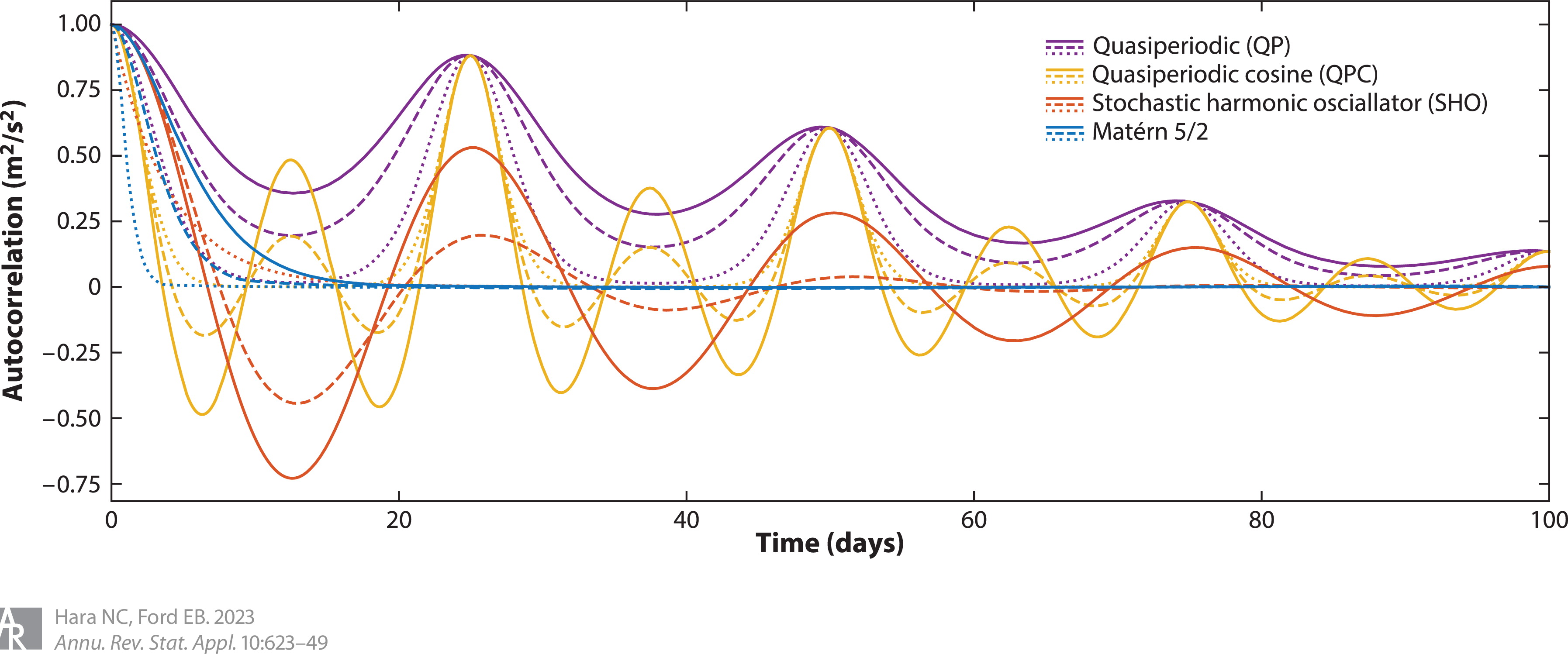
Figure 6: Kernel functions: functions of the time lag $\Delta t$ between two observations. The covariance matrix $\mathbf{V}$ in Eq. (10) is such that its element $i,j$ is a sum of kernel functions evaluated in $\Delta t=t_{i}-t_{j}$. Each color corresponds to a different family of kernels: Quasi periodic (QP Aigrain et al., 2012, Haywood et al., 2014), quasi-periodic cosine (QPC Perger et al., 2021), stochastic harmonic oscillator (Foreman-Mackey et al., 2017), Matérn 5/2 (Foreman-Mackey et al., 2017, Gilbertson et al., 2020). Each family has several parameters, including an amplitude, a time-scale, and for all but Matérn 5/2, a period. They have additionally shape parameters and plain, dashed and dotted correspond to different values of this shape parameters. The periods are taken as 25 days, close to the Sun rotational period, and all kernels are normalized so that they are equal to 1 in $\Delta t=0$. These different kernels model different phenomena (see §2.4.1). The QP kernel is well suited to represent stellar rotational effects due to convective blueshift inhibition with various stellar inclinations. QPCs model the fact that spots appear preferentially on stellar longitudes with a 180^∘ phase shift in Sun-like stars (QPC Borgniet et al., 2015, Spergel et al., 2015). SHO kernels have take negative values, this type of anticorrelation arises due to the breaking of imbalance of flux of the approaching and receding limb, and certain parameter values correspond to a super-Lorentzian power spectral density used to model granulation (Foreman-Mackey et al., 2017, Gilbertson et al., 2020). Matérn 5/2 are efficient tio model RV induced by spots and faculae with a lifetime lower than the rotation period (Gilbertson et al., 2020). Explicit kernels expression and values of the parameters are given in Appendix E.2.

Gaussian processes were introduced to the exoplanet community in Aigrain et al. (2012). They showed that when nearly contemporaneous photometric and RV observations of a star are available, the effect of one stellar spot on RV can be predicted through the photometric flux and its derivative. For most targets, continuous photometric measurements are unavailable. One can estimate the derivative of the flux at any time using Gaussian processes (GPs). These are stochastic processes $G(\mathbf{t})$, function of a variable $\mathbf{t}$ such that for any $n$ values of $\mathbf{t}$, $\mathbf{t}_{1},...,\mathbf{t}_{n}$, $(G(\mathbf{t}_{1}),...,G(\mathbf{t}_{n}))$ follows a multivariate Gaussian distribution. In general, $\mathbf{t}$ can be a vector, but for our purpose, we define it as the time $t$. This implies that the GP is defined by two quantities: its mean $m(t)$ and kernel, $k(t,t^{\prime})$, equal to the covariance of $G(t)$ and $G(t^{\prime})$ (Rasmussen & Williams, 2005, Aigrain & Foreman-Mackey, 2022).

Aigrain et al. (2012) use photometric data to predict the RV variation. We can go a step further and analyze RV and ancillary indicators simultaneously by building a likelihood $p(\mathbf{RV},\mathbf{I}\mid\mathbf{D})$, typically in the Gaussian process (GP) framework. RVs and ancillary indicators are expressed as linear combinations of one or several latent Gaussian processes and their derivatives (Rajpaul et al., 2015, Gilbertson et al., 2020, Gordon et al., 2020, Barragán et al., 2022, Delisle et al., 2022, Tran et al., 2023). Since $G(t+\Delta t)\approx G(t)+\dot{G}(t)\Delta t$, using the derivative can account for small phase shifts between RV and indicators. The data $\mathbf{y}$ in Eq. 10 is then the concatenation of the RV vector and ancillary indicators. Fig. 7 shows an example of RV and ancillary indicators modeled simultaneously with a GP and its derivative.

Representing RV and ancillary indicators as a linear combination of a GP and its derivative is only one way to specify the covariance in Eq. 10, other options have been proposed. For example, the GP framework can be used to model simultaneously the RVs derived in different spectral bands (Cale et al., 2021). The kernel of the extended data $\mathbf{y}$ can also be based on explicit physical models of the star (Luger et al., 2021b, a, Hara & Delisle, 2023). Furthermore, the assumption that the likelihood is Gaussian and stationary can be relaxed. Hara & Delisle (2023) quantifies non Gaussianity with an analytical model of stellar variability. Camacho et al. (2023) model the RV and ancillary indicator time series in a GP regression network. It allows, in particular, consideration of noise with heavy tails and offers ways to account for non-stationarity due to the magnetic cycle.

Evaluating the likelihood Eqn. 10 for certain values of the parameters requires the log determinant of $\mathbf{V}(\bm{\mathord{\mkern 1.3mu\ThisStyle{\mbox{\hskip 14.03473pt{1 0 -.25 1}\hbox to0.0pt{\hss\leavevmode\hbox{$\SavedStyle\eta$}}}}\mkern-1.3mu}})$ and computing $\{\mathbf{y}-\mathbf{g}(\mathbf{t};\bm{\mathord{\mkern 1.3mu\ThisStyle{\mbox{\hskip 13.76387pt{1 0 -.25 1}\hbox to0.0pt{\hss\leavevmode\hbox{$\SavedStyle\theta$}}}}\mkern-1.3mu}})\}^{T}\mathbf{V}^{-1}(\bm{\mathord{\mkern 1.3mu\ThisStyle{\mbox{\hskip 14.03473pt{1 0 -.25 1}\hbox to0.0pt{\hss\leavevmode\hbox{$\SavedStyle\eta$}}}}\mkern-1.3mu}})\{\mathbf{y}-\mathbf{g}(\mathbf{t};\bm{\mathord{\mkern 1.3mu\ThisStyle{\mbox{\hskip 13.76387pt{1 0 -.25 1}\hbox to0.0pt{\hss\leavevmode\hbox{$\SavedStyle\theta$}}}}\mkern-1.3mu}})\}$. With standard algorithms the computational cost scales as $O(N^{3})$ with the size $N$ of the dataset $\mathbf{y}$, and becomes prohibitive for $N\gtrsim 10^{3}$. This prevents using many indicators on stars with hundreds of points, or analysing the tens of thousands of RV measurements on the Sun. Fortunately, for certain choices of the kernel, the covariance matrix has a “semi-separable” expression and then the computational cost scales as $O(N)$ (the CELERITE framework, Foreman-Mackey et al., 2017, Foreman-Mackey, 2018). Similarly, TemporalGPs.jl allows for $O(N)$ computation of a broad class of 1-d kernel functions in Julia. The CELERITE framework is generalised by Delisle et al. (2020b) to the S+LEAF framework, which models covariances as a sum of semi-separable and “LEAF matrices”. Quasi-separable kernels provide even greater flexibility for modeling multivariable timeseries (tinygp ). Delisle et al. (2022) show that if RV and ancillary indicators are linear combinations of a Gaussian process $G(t)$ and its derivatives, and the covariance of $G(t)$ has a S+LEAF form, the computation of the likelihood of the augmented data is still $O(N)$.

The merits of the different noise models can be evaluated through Bayesian model comparison (see §4.3), as in Ahrer et al. (2021), Faria et al. (2022), Suárez Mascareño et al. (2021), alternatively Bayesian model averaging can be used (Hara et al., 2022a).

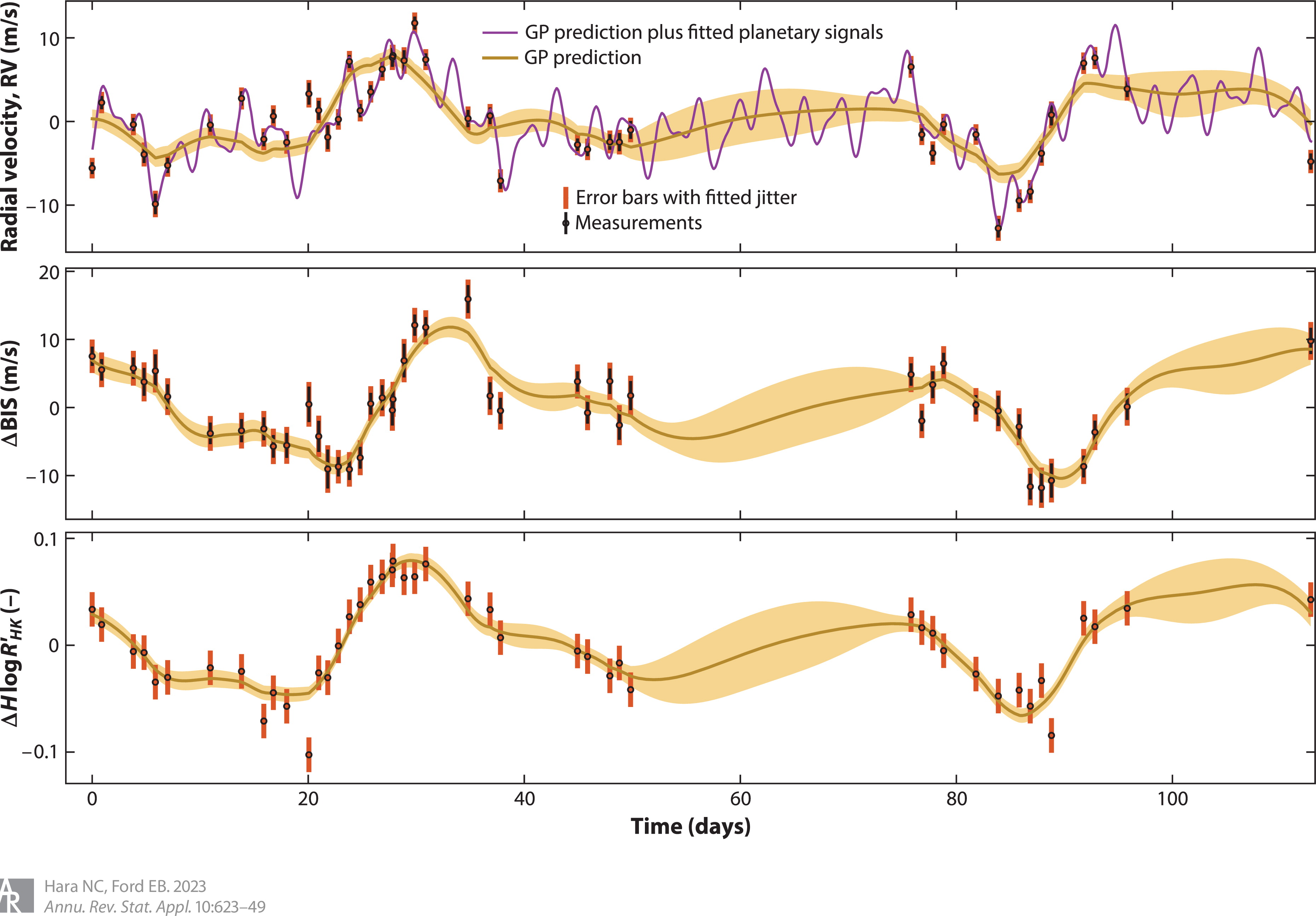
Figure 7: Gaussian process regression applied to the time series of RV, and ancillary indicators $\Delta$BIS (Queloz et al., 2001) and $\Delta\log R^{\prime}_{\mathrm{HK}}$ (Noyes, 1984) of 46 measurements obtained on the star TOI 178 with the ESPRESSO instrument (Leleu et al., 2021). Each of the three time series $y_{i}(t)$, $i=1,2,3$ is represented by a model $y_{i}(t)=\alpha_{i}G(t)+\beta_{i}\dot{G}(t)+\epsilon_{m}(t)+\epsilon_{J}(t)$. The Gaussian process $G$ has a stochastic harmonic oscillator (SHO) kernel (Foreman-Mackey et al., 2017) with three parameters, fitted with the S+LEAF package (Delisle et al., 2022). The processes $\epsilon^{m}(t)$ and $\epsilon^{J}(t)$ represent the measurement error and jitter. We represent with a brown line the mean of the posterior predictive distribution for each time series, and the shaded yellow areas represent $\pm$1 standard deviation of $\alpha_{i}G(t)+\beta_{i}\dot{G}(t)$. The purple curve represents the variations predicted by the best-fit Keplerian model for the planet, whose presence is confirmed by transits (Leleu et al., 2021). Other abbreviations: BIS, bisector inverse slope; $\Delta\log R^{\prime}_{\mathrm{HK}}$, ancillary indicator derived from each spectrum.

6 ANALYSIS METHODS: DEEPER LEVELS

So far, we have seen different methods to detect planets and estimate their orbital elements given priors and likelihood in $\S$4. We have seen how the model can be built based on a certain reduction of the data in $\S$5. We now present techniques to extract physical information from the spectra.

Our goal is to identify conceptual similarities between different methods, rather than to assess their performances. While the community has begun to compare methods (Zhao et al., 2022), proper evaluations are challenging since one does not know the true RV for real stars due to potential undetected planets (except for our Sun; Collier Cameron et al., 2019, Dumusque et al., 2020, Lin et al., 2022). We suggest metrics to compare approaches in §7.

6.1 Estimating RV

For a fixed stellar spectrum, the RV is well defined and can be extracted from the spectrum using multiple techniques described below. However, at the sub-m/s (or a few $\mathrm{RV}_{\oplus}$), level, the shape of the spectrum changes, so, there is no unambiguous definition of RV, and each method to estimate it relies on more or less explicit assumptions. Depending on how this shape change is modelled, the estimate of the Doppler shift changes.

Three main families of methods for extracting the velocity in each spectrum separately are in use. As discussed in §3, the historic method consists of cross-correlating the spectrum with an idealised mask (Baranne et al., 1979, Pepe et al., 2002). Denoting by $f(\lambda)$ the flux as a function of the wavelength $\Lambda$,

$$\mathrm{CCF}(\Delta\lambda)=f\ast\mathrm{Mask}(\Delta\lambda)$$ (14)

where $\ast$ is the convolution operator. This method can be viewed as computing an average line shape. Each line contributes to improving the SNR, but also contributes a bias since true line wavelengths are unknown. Additionally, the CCF loses information about differences in shapes of each line. Often, many lines are excluded from the CCF mask to reduce contamination of lines likely to contribute significant bias. Alternatively, Lienhard et al. (2022) proposes a least-square deconvolution technique to estimate a common spectral line profile.

A second approach, template matching, consists in measuring the RV based on a template or model spectrum and a Taylor expansion for the spectrum as a function of velocity (Connes, 1985, Bouchy et al., 2001, Anglada-Escudé & Tuomi, 2012, Astudillo-Defru et al., 2015, Jones et al., 2022, Silva et al., 2022). Related work has been done by Cretignier et al. (2022). This approach is based on the approximation

$$f(\lambda)\simeq f_{0}(\lambda)+\frac{RV}{c}\frac{\operatorname{d}f_{0}}{\operatorname{d}\log\lambda}\left(\lambda\right),$$ (15)

where $f_{0}(\lambda)$ is a reference spectrum and $c$ is the speed of light. Both the CCF and template matching approaches aim to reduce the impact of stellar variability by careful selection of lines/wavelengths for inclusion, but lack a mechanism to recognize stellar variability. Some authors measure the RV of each line separately (Dumusque, 2018, Artigau et al., 2022) (or $\sim~{}2$Å“chunk” of the spectrum), and compute a weighted average RV after a statistical rejection of outliers, or do independent RV estimates in several bandwidths (Feng et al., 2017, Zechmeister et al., 2018). The rationale is to disentangle signals which affect all wavelengths identically (planet candidates) from other signals.

A third approach builds a forward model of the spectrum,

$$f(\lambda^{o})=\left[f_{0}(\lambda^{bc})+\frac{RV}{c}\frac{df_{o}}{d\log\lambda}(\lambda^{bc})\right]T(\lambda^{o})\ast IP(\lambda^{o}),$$ (16)

where$f(\lambda^{0})$ is the spectrum in the observer frame, $\lambda^{bc}(t)=\lambda^{o}\{1+v_{bc}(t)/c\}/\sqrt{1-v_{bc}^{2}(t)/c^{2}}$ is the wavelength in a frame that accounts for $v_{bc}(t)$, the known motion of the observatory relative to the solar system barycenter (the “barycentric correction”), where $T(\cdot)$ is an atmospheric transmission profile, and $IP(\cdot)$ is the instrument response. Variations on forward modeling have focused on telluric effects (Butler et al., 1996, Hirano et al., 2020) or on stellar variability (Bedell et al., 2019, Gilbertson et al., 2020, Jones et al., 2022). Ongoing research is developing computational tractable approaches for including both simultaneously (e.g., StellarSpectraObservationFitting.jl).

As methods become more sophisticated, the estimation of the velocity and fitting of spectral shape tend to be made simultaneously on the time series of spectra. In principle, this mitigates the chance that the Doppler shift is contaminated by shape changes, and uses temporal structure to further constrain activity.

6.2 Estimating nuisance RV signals

To put Eq. (9) into practice, one must specify a statistical model for $p(\mathbf{I},\mathbf{RV}_{\mathrm{contam}}\mid\bm{\mathord{\mkern 1.3mu\ThisStyle{\mbox{\hskip 13.76387pt{1 0 -.25 1}\hbox to0.0pt{\hss\leavevmode\hbox{$\SavedStyle\theta$}}}}\mkern-1.3mu}},\bm{\mathord{\mkern 1.3mu\ThisStyle{\mbox{\hskip 14.03473pt{1 0 -.25 1}\hbox to0.0pt{\hss\leavevmode\hbox{$\SavedStyle\eta$}}}}\mkern-1.3mu}})$. First, one chooses the method of dimension reduction to obtain $\mathbf{I}$, and then a form for the likelihood which describes $\mathbf{I}$ and $\mathbf{RV}_{\mathrm{contam}}$.

Dimension reduction has been applied to real and synthetic spectra. Davis et al. (2017) applied PCA to spectra generated with SOAP 2.0. Since real stellar spectra are more complicated, their analysis provides a lower limit on the number of PCA components needed to accurately reconstruct solar spectra (ranging from 1 to 4 depending on the spectral resolution and SNR). Analysis of solar data suggests that only 6-13 basis vectors are necessary to model solar variability at the resolution and SNR of HARPS-N observations, and at least four of those are clearly linked to effects due to the instrument or unique to sun-as-a-star observations (Collier Cameron et al., 2021). Together, these suggest that reducing spectra to an RV and two to six indicators is a fruitful direction for future research.

Dimension reduction and estimation of contaminating RV can be done simultaneously. Existing methods extract ancillary indicators either in each spectrum separately, from a time series of CCFs (or other summaries of the spectra), or from the time series of spectra themselves. In the following subsections we describe the associated methods.

6.2.1 Extraction spectrum by spectrum

Some methods extract activity indicators from each spectrum separately. For example, one can measure line shapes (or deviations from their time-average). Shape line indicators were first extracted from the CCF, in particular its asymmetry (Queloz et al., 2001) and width (Queloz et al., 2009). Other indicators involve fitting Gaussian distributions on each side of the CCF (Figueira et al., 2013). Holzer et al. (2021) fit a superposition of Gauss–Hermite functions to each line to build shape indicators.

Another approach is to measure properties of specific absorption lines of interest. The utility of different lines depends on the effective temperature of the host star. For sun-like stars, $\log R^{\prime}_{HK}$ and the so-called $S$-index are popular magnetic activity indicators based on emission in the core of the Calcium II H&K lines (Noyes, 1984, Wright et al., 2004). For cooler stars, the $H\alpha$ line is a more useful indicator (Kürster et al., 2003, Robertson et al., 2016). The unsigned magnetic field estimated from the spectrum can be a powerful indicator of $\operatorname{RV}_{\mathrm{contam}}$ (Haywood et al., 2020) and might generalize better than any individual line.

Santerne et al. (2015) and Lanza et al. (2018) find that activity indicators can have relatively weak correlations with RV signals contaminating the data. One contributing factor is the expected time lag between RVs and other indicators, noted in the case of RV and photometry (Queloz et al., 2001, Santos et al., 2003, Queloz et al., 2009) and other indicators (Suárez Mascareño et al., 2017). This time lag can be partially mitigated in models where the derivative of the latent Gaussian process appears (Rajpaul et al., 2015, Delisle et al., 2022) or with adaptive correlation (Simola et al., 2022).

6.2.2 Methods using stellar variability indicators

More generally, spectra can be reduced to a set of summary statistics that serve as stellar variability indicators and their time series can be analyzed jointly with the RVs. By utilizing temporal information, we may obtain less noisy indicators.

The most common reduction is to compute the CCF. However, good indicators should be insensitive to true Doppler shifts, so Collier Cameron et al. (2021) proposed Scalpels to analyze the autocorrelation of the CCF. The resulting time series of CCF autocorrelations are analyzed with a PCA and the PCA scores are used as variability indicators. Since the autocorrelation function is insensitive to shifts, true Doppler shifts will not affect the resulting variability indicators. de Beurs et al. (2022) explored more flexible supervised learning approaches to predicting $\operatorname{RV}_{\mathrm{contam}}$ from a training data set, either simulated or solar data CCFs. It is unclear whether the greater flexibility of neural networks will outweight their added complexity and difficulty of interpretation relative to linear regression or Scalpels, particularly given the limited size of datasets available for stars other than the Sun.

Cretignier et al. (2022) transform the spectra into “shells” instead of CCFs, in an effort to reduce the amount of information lost when averaging lines of different depths. The PCA scores for the shell are used as spectral indicators, but are first orthonormalised with respect to the shell corresponding to a pure Doppler shift.

More research is needed to develop effective means of comparing choices of summary statistics, variability indicators and corresponding likelihoods. Several methods were explored in the EXPRES Stellar Signals Project, where several teams analysed observations of four stars by EXPRES (Zhao et al., 2022). One key finding was that while many methods could reduce the root mean square RMS RV of observations, the estimates of $\operatorname{RV}_{\mathrm{contam}}$ differ significantly across methods. Without knowing the true velocity, it was impossible to determine which methods are best. In §7.2, we present several ideas for a robust comparison of the different methods leveraging the existing and upcoming RV observations of the Sun with different instruments.

Sun-as-a-star observations allow the testing and validation of methods for mitigating stellar variability. Three methods, Scalpels (Collier Cameron et al., 2021), linear regression on CCFs and neural networks (de Beurs et al., 2022) have been shown to significantly reduce the level of RV variability in solar observations. Existing and upcoming comparisons of Sun-as-a-star observations from multiple instruments, including a new generation of more highly stabilized spectrographs, will help disentangling solar RV variations due to the solar variability and from instrument specific signals, and refine the comparisons of different analysis methods.

6.2.3 Methods using the time series of spectra

Rajpaul et al. (2020) propose an alternative approach of measuring a $\Delta\operatorname{RV}$ from each pair of spectra and reconstructing the RV time series (modulo a constant), while giving greater weight to pairs that are more similar. In order to reduce the computational cost, they split the spectra into many small chunks to be analyzed separately.

In principle, one could perform inference on the entire spectroscopic time series. Jones et al. (2022) introduced Doppler-constrained PCA on the time series of spectra to characterize stellar variability and provided a proof of concept on simulated solar observations. Bedell et al. (2019) applied a similar method to real observations, emphasizing modeling of telluric contamination and neglecting stellar variability. They regularized the variables using $\ell_{1}$ and $\ell_{2}$ norm constraints. More recent work has developed computationally efficient implementations that simultaneously model both stellar and telluric variability, as well as accounting for the instrumental profile and allowing for physically-informed regularization schemes.

7 CONCLUSION

7.1 Summary

RV is poised to play a key role in the study of exoplanets in the next decade as a primary way to measure their masses; to detect interesting, nontransiting planets; to have a more complete view of planetary system architectures; and to provide targets whose atmospheres will be further characterized by spectro-imaging or interferometry. Currently, characterizing an Earth twin is out of reach, and improving data analysis techniques will play a fundamental role.

We presented the different steps of RV data analysis, separating them in three problems (see Section 3): ($a$) reducing the information of the spectrum into an RV time series, ($b$) modeling nuisance signals and the prior information on planetary and nuisance parameters, and ($c$) deciding how many planets are present and what their orbital elements are. Each of these steps requires numerical methods, where convergence should be carefully checked. Since there are multiple reasonable choices for $a$, $b$, and $c$, researchers should perform multiple analyses with different assumptions to determine whether key conclusions are sensitive to these choices, especially of the likelihood and prior.

7.2 Future work

The exoplanet community is now well-equipped to analyze RV observations when planetary signals dominate stellar and instrumental variability. When these planetary signals and corrupting ones are of similar amplitude, the fact that different methods yield different results (Zhao et al., 2022) shows that more work remains to be done. We believe that further research in steps $a$ and $b$ is crucial.

The ability of RVs to detect and measure the mass of potential Earth twins is critically linked to how precisely the contaminating RV signals, the RV signal not due to the motion of the center of mass of the star ($\operatorname{RV}_{\mathrm{contam}}$ in Equations (7)-(8)), can be predicted and how accurately the uncertainty on these predictions can be quantified. Correcting these signals can be done either in a statistical framework by building a likelihood function or with supervised learning techniques trained to predict the RV contamination signal from spectral shapes. The new models may be data-driven or physics-driven, especially for RV signals originating from the star, for which there is a substantial modeling effort (see Appendix B.2) yet to be translated to data analysis techniques. Further research in step a is also required to ensure that all the information contained in the spectra is used and that the RV and indicators derived are reliable summary statistics.

We believe that one of the most critical question is how to validate choices for each step as effective tools for detecting and characterizing low mass planets in the presence of stellar variability. We propose three ways forward, the first two concerning the validation of reduction and modelling (step $a$ and $b$), and the third the whole process ($a$–$c$).

The first approach is Bayesian model comparison, to evaluate the relative merits of different stellar activity and instrument systematics models. Ideally this would be applied to datasets with no ambiguity on the presence or not of planetary signals. For example, since we know the true solar velocity, we can evaluate the signal $\mathrm{RV}_{\mathrm{contam}}$ of each method applied to sun-as-a-star observations. A similar approach may be possible for some other stars hosting a massive planet on an eccentric orbit, since one can exclude the possibility of additional planets for a wide range of orbital periods based on orbital stability considerations (Brewer et al., 2020, Stalport et al., 2022). Large and computationally demanding computer models could provide data for training and testing models, though they must be validated beforehand. The observations of the Sun by different high precision spectrographs can be leveraged to disentangle instrument specific noise from stellar variability.

Second, for stars where one acquires a sufficiently large number of observations, one could evaluate the accuracy and precision of a model mitigating stellar variability via its ability to predict $\operatorname{RV}_{\mathrm{contam}}$ (see Eq. (7)) and stellar variability indicators at times not used in the training of the model. Given multiple processes operating on a variety of timescales, one must carefully design the training, testing and validation procedure. For example, if one obtained multiple spectra per night and stellar variability were operating on timescales of weeks, then one could trivially predict the $\operatorname{RV}_{\mathrm{contam}}$ from another observation on the same night, without learning how to recognize stellar variability in line shapes or depth ratios. Additionally, one must be careful that cross validation is not undermined by researchers effectively trying many strategies and reporting results from those that appear to work best.

The two approaches above pertain to validating models for contaminating signals. The most convincing method for validating models may be via planet injection-recovery tests. One group of researchers would work on injecting planets in real or simulated datasets. Another group of researchers would blindly analyze large ensembles of simulated datasets. This would allow each proposed data reduction method and likelihood to be evaluated differentially, i.e., comparing the inferred velocities from multiple simulated data sets generated from the same true data set. Given the inevitable arbitrary nature of labeling some signals as “confident” exoplanet detections, it is not sufficient for teams to label which signals they believe is due to an exoplanet. Instead, we recommend that they provide a list of all putative signals along with a quantiative measure of the signals’ statistical significances (FAP, Bayes factor, FIP, see §4). Then, the number of false detections can be computed as a function of the number or properties of missed planets. To generate the data, one approach would be to remove telluric and instrumental effects, introduce a larger number of artificial Doppler shifts, reinject the telluric and instrumental effects, and generate many new synthetic data sets (perhaps adding additional noise along the way). One must be careful in implementing this approach, as an error in the injection process could become a feature learned by data-driven methods that would not be available for realistic data sets.

In this review, we adopted the viewpoint that RV data analysis should be viewed as a whole from the most basic data products to the final decisions. It will be crucial to build accurate instrument systematics and stellar noise models, to leverage as much as possible the information contained in the spectra, and to build reliable metrics to validate the different methods. Progress will most likely stem from the combination of a deep knowledge of the instruments and astronomical context combined with formal approaches, which will provide adequate tools to represent and analyze the data.

Appendix A DEFINITIONS

For convenience we reproduce here the formalism used in the main text. We denote by $\operatorname{RV}(t)$ the radial velocity (RV) of a given star due to a motion of its center of the mass at time $t$. We denote by $\operatorname{RV}_{\mathrm{contam}}(t)$ the RV signal caused by stellar variability and instrument systematics, and $\epsilon(t)$, the photon noise. From an estimated Doppler shift of the spectrum, the radial velocity measurement estimated at time $t$, $\widehat{\operatorname{RV}(t)}$, is

$$\widehat{\operatorname{RV}(t)} =\operatorname{RV}(t)+\operatorname{RV}_{\mathrm{contam}}(t)+\epsilon(t).$$ (17)

$$\operatorname{RV}(t) =\operatorname{RV}_{\mathrm{planets}}(t)+\operatorname{RV}_{\mathrm{g}}(t)$$ (18)

where $\operatorname{RV}_{\mathrm{planets}}(t)$ is the RV signal caused by the planets and $\operatorname{RV}_{\mathrm{g}}(t)$ is the RV signal caused by other gravitational effects, such as the proper motion of the star in the galaxy, or the influence of another star. The time series of radial measured velocities is denoted by $\widehat{\mathbf{RV}}=(\widehat{\operatorname{RV}}(t_{i}))_{i=1,..,N}$.

Let us suppose that a star is observed by a spectrograph at $N$ different times, $t_{i},i=1,..,N$. We denote by $\mathbf{D}(t_{i})$ the lowest level data product at time $t_{i}$, the fluxes measured on the spectrograph detector of the and various housekeeping data (temperature, pressure etc). In principle, we could base our inference on the time series $\mathbf{D}=(\mathbf{D}(t_{i}))_{i=1,..N}$. Loosely speaking, we want to use non Doppler variations of $\mathbf{D}$ to estimate as closely as possible $\operatorname{RV}_{\mathrm{contam}}(t)$, in particular the variation of the shape of spectral lines, and color-dependent effects. We can also leverage the fact that, unless there are strong dynamical interactions between planets, the planetary signals are purely periodic, but systematics and stellar activity are not.

We denote by $\bm{\mathord{\mkern 1.3mu\ThisStyle{\mbox{\hskip 13.76387pt{1 0 -.25 1}\hbox to0.0pt{\hss\leavevmode\hbox{$\SavedStyle\theta$}}}}\mkern-1.3mu}}$ the parameters of the planets orbiting the star and $\bm{\mathord{\mkern 1.3mu\ThisStyle{\mbox{\hskip 14.03473pt{1 0 -.25 1}\hbox to0.0pt{\hss\leavevmode\hbox{$\SavedStyle\eta$}}}}\mkern-1.3mu}}$ all other parameters describing the signal (offset, noise level, parameters of the noise kernel), respectively. We have $\bm{\mathord{\mkern 1.3mu\ThisStyle{\mbox{\hskip 13.76387pt{1 0 -.25 1}\hbox to0.0pt{\hss\leavevmode\hbox{$\SavedStyle\theta$}}}}\mkern-1.3mu}}=(\bm{\mathord{\mkern 1.3mu\ThisStyle{\mbox{\hskip 13.76387pt{1 0 -.25 1}\hbox to0.0pt{\hss\leavevmode\hbox{$\SavedStyle\theta$}}}}\mkern-1.3mu}}_{1},...,\bm{\mathord{\mkern 1.3mu\ThisStyle{\mbox{\hskip 13.76387pt{1 0 -.25 1}\hbox to0.0pt{\hss\leavevmode\hbox{$\SavedStyle\theta$}}}}\mkern-1.3mu}}_{n}$) where $n$ is the number of planets (which is also a variable) and $\bm{\mathord{\mkern 1.3mu\ThisStyle{\mbox{\hskip 13.76387pt{1 0 -.25 1}\hbox to0.0pt{\hss\leavevmode\hbox{$\SavedStyle\theta$}}}}\mkern-1.3mu}}_{j}$ the orbital elements of the planet indexed by $j$ (see Eq. (23)). $\mathbf{D}$ is reduced to an estimate of the RV time series $\widehat{\mathbf{RV}}$ and ancillary indicators $\mathbf{I}=(\mathbf{I}_{j}(t_{i}))_{j=1..p,i=1..N}$, are $p$ time series of length $N$, summarizing the variations of shape of the spectrum. The goal is not to loose too much information in the reduction process. We thus want

$$p(\bm{\mathord{\mkern 1.3mu\ThisStyle{\mbox{\hskip 13.76387pt{1 0 -.25 1}\hbox to0.0pt{\hss\leavevmode\hbox{$\SavedStyle\theta$}}}}\mkern-1.3mu}},\bm{\mathord{\mkern 1.3mu\ThisStyle{\mbox{\hskip 14.03473pt{1 0 -.25 1}\hbox to0.0pt{\hss\leavevmode\hbox{$\SavedStyle\eta$}}}}\mkern-1.3mu}}\mid\mathbf{D})\approx p(\bm{\mathord{\mkern 1.3mu\ThisStyle{\mbox{\hskip 13.76387pt{1 0 -.25 1}\hbox to0.0pt{\hss\leavevmode\hbox{$\SavedStyle\theta$}}}}\mkern-1.3mu}},\bm{\mathord{\mkern 1.3mu\ThisStyle{\mbox{\hskip 14.03473pt{1 0 -.25 1}\hbox to0.0pt{\hss\leavevmode\hbox{$\SavedStyle\eta$}}}}\mkern-1.3mu}}\mid\mathbf{I},\widehat{\mathbf{RV}}),$$ (19)

and thanks to the Bayes formula, we have

$$p(\bm{\mathord{\mkern 1.3mu\ThisStyle{\mbox{\hskip 13.76387pt{1 0 -.25 1}\hbox to0.0pt{\hss\leavevmode\hbox{$\SavedStyle\theta$}}}}\mkern-1.3mu}},\bm{\mathord{\mkern 1.3mu\ThisStyle{\mbox{\hskip 14.03473pt{1 0 -.25 1}\hbox to0.0pt{\hss\leavevmode\hbox{$\SavedStyle\eta$}}}}\mkern-1.3mu}}\mid\mathbf{I},\widehat{\mathbf{RV}})=\frac{p(\mathbf{I},\widehat{\mathbf{RV}}\mid\bm{\mathord{\mkern 1.3mu\ThisStyle{\mbox{\hskip 13.76387pt{1 0 -.25 1}\hbox to0.0pt{\hss\leavevmode\hbox{$\SavedStyle\theta$}}}}\mkern-1.3mu}},\bm{\mathord{\mkern 1.3mu\ThisStyle{\mbox{\hskip 14.03473pt{1 0 -.25 1}\hbox to0.0pt{\hss\leavevmode\hbox{$\SavedStyle\eta$}}}}\mkern-1.3mu}})p(\bm{\mathord{\mkern 1.3mu\ThisStyle{\mbox{\hskip 13.76387pt{1 0 -.25 1}\hbox to0.0pt{\hss\leavevmode\hbox{$\SavedStyle\theta$}}}}\mkern-1.3mu}},\bm{\mathord{\mkern 1.3mu\ThisStyle{\mbox{\hskip 14.03473pt{1 0 -.25 1}\hbox to0.0pt{\hss\leavevmode\hbox{$\SavedStyle\eta$}}}}\mkern-1.3mu}})}{p(\mathbf{I},\widehat{\mathbf{RV}})}=\frac{p(\mathbf{I},\mathbf{RV}_{\mathrm{contam}}+\bm{\mathord{\mkern 1.3mu\ThisStyle{\mbox{\hskip 13.12846pt{1 0 -.25 1}\hbox to0.0pt{\hss\leavevmode\hbox{$\SavedStyle\epsilon$}}}}\mkern-1.3mu}}\mid\bm{\mathord{\mkern 1.3mu\ThisStyle{\mbox{\hskip 13.76387pt{1 0 -.25 1}\hbox to0.0pt{\hss\leavevmode\hbox{$\SavedStyle\theta$}}}}\mkern-1.3mu}},\bm{\mathord{\mkern 1.3mu\ThisStyle{\mbox{\hskip 14.03473pt{1 0 -.25 1}\hbox to0.0pt{\hss\leavevmode\hbox{$\SavedStyle\eta$}}}}\mkern-1.3mu}})p(\bm{\mathord{\mkern 1.3mu\ThisStyle{\mbox{\hskip 13.76387pt{1 0 -.25 1}\hbox to0.0pt{\hss\leavevmode\hbox{$\SavedStyle\theta$}}}}\mkern-1.3mu}},\bm{\mathord{\mkern 1.3mu\ThisStyle{\mbox{\hskip 14.03473pt{1 0 -.25 1}\hbox to0.0pt{\hss\leavevmode\hbox{$\SavedStyle\eta$}}}}\mkern-1.3mu}})}{p(\mathbf{I},\widehat{\mathbf{RV}})}.$$ (20)

The last equality comes from the fact that $\operatorname{RV}(t)$ depends deterministically on $\bm{\mathord{\mkern 1.3mu\ThisStyle{\mbox{\hskip 13.76387pt{1 0 -.25 1}\hbox to0.0pt{\hss\leavevmode\hbox{$\SavedStyle\theta$}}}}\mkern-1.3mu}},\bm{\mathord{\mkern 1.3mu\ThisStyle{\mbox{\hskip 14.03473pt{1 0 -.25 1}\hbox to0.0pt{\hss\leavevmode\hbox{$\SavedStyle\eta$}}}}\mkern-1.3mu}}$. Below, we denote $\mathbf{y}=(\widehat{\mathbf{RV}},\mathbf{I})$, potentially with $\mathbf{I}$ = 0. We will refer to $p(\bm{\mathord{\mkern 1.3mu\ThisStyle{\mbox{\hskip 13.76387pt{1 0 -.25 1}\hbox to0.0pt{\hss\leavevmode\hbox{$\SavedStyle\theta$}}}}\mkern-1.3mu}},\bm{\mathord{\mkern 1.3mu\ThisStyle{\mbox{\hskip 14.03473pt{1 0 -.25 1}\hbox to0.0pt{\hss\leavevmode\hbox{$\SavedStyle\eta$}}}}\mkern-1.3mu}})$ as the prior distribution and $p(\mathbf{y}\mid\bm{\mathord{\mkern 1.3mu\ThisStyle{\mbox{\hskip 13.76387pt{1 0 -.25 1}\hbox to0.0pt{\hss\leavevmode\hbox{$\SavedStyle\theta$}}}}\mkern-1.3mu}},\bm{\mathord{\mkern 1.3mu\ThisStyle{\mbox{\hskip 14.03473pt{1 0 -.25 1}\hbox to0.0pt{\hss\leavevmode\hbox{$\SavedStyle\eta$}}}}\mkern-1.3mu}})$ as the likelihood. The notation $p(\mathbf{y}\mid\bm{\mathord{\mkern 1.3mu\ThisStyle{\mbox{\hskip 13.76387pt{1 0 -.25 1}\hbox to0.0pt{\hss\leavevmode\hbox{$\SavedStyle\theta$}}}}\mkern-1.3mu}},\bm{\mathord{\mkern 1.3mu\ThisStyle{\mbox{\hskip 14.03473pt{1 0 -.25 1}\hbox to0.0pt{\hss\leavevmode\hbox{$\SavedStyle\eta$}}}}\mkern-1.3mu}},n)$ refers to the posterior restricted to models with exactly $n$ planets.

The likelihood is commonly assumed to be Gaussian,

$$\mathcal{L}\equiv p(\mathbf{y}\mid\bm{\mathord{\mkern 1.3mu\ThisStyle{\mbox{\hskip 13.76387pt{1 0 -.25 1}\hbox to0.0pt{\hss\leavevmode\hbox{$\SavedStyle\theta$}}}}\mkern-1.3mu}},\bm{\mathord{\mkern 1.3mu\ThisStyle{\mbox{\hskip 14.03473pt{1 0 -.25 1}\hbox to0.0pt{\hss\leavevmode\hbox{$\SavedStyle\eta$}}}}\mkern-1.3mu}})=\frac{\operatorname{e}^{-\frac{1}{2}\left[\mathbf{y}-\mathbf{g}(\mathbf{t};\bm{\mathord{\mkern 1.3mu\ThisStyle{\mbox{\hskip 9.6347pt{1 0 -.25 1}\hbox to0.0pt{\hss\leavevmode\hbox{$\SavedStyle\theta$}}}}\mkern-1.3mu}},\bm{\mathord{\mkern 1.3mu\ThisStyle{\mbox{\hskip 9.82431pt{1 0 -.25 1}\hbox to0.0pt{\hss\leavevmode\hbox{$\SavedStyle\eta$}}}}\mkern-1.3mu}})\right]^{T}\mathbf{V(\bm{\mathord{\mkern 1.3mu\ThisStyle{\mbox{\hskip 9.82431pt{1 0 -.25 1}\hbox to0.0pt{\hss\leavevmode\hbox{$\SavedStyle\eta$}}}}\mkern-1.3mu}})}^{-1}\left[\mathbf{y}-\mathbf{g}(\mathbf{t};\bm{\mathord{\mkern 1.3mu\ThisStyle{\mbox{\hskip 9.6347pt{1 0 -.25 1}\hbox to0.0pt{\hss\leavevmode\hbox{$\SavedStyle\theta$}}}}\mkern-1.3mu}},\bm{\mathord{\mkern 1.3mu\ThisStyle{\mbox{\hskip 9.82431pt{1 0 -.25 1}\hbox to0.0pt{\hss\leavevmode\hbox{$\SavedStyle\eta$}}}}\mkern-1.3mu}})\right]}}{\sqrt{(2\pi)^{N}|\mathbf{V}(\bm{\mathord{\mkern 1.3mu\ThisStyle{\mbox{\hskip 14.03473pt{1 0 -.25 1}\hbox to0.0pt{\hss\leavevmode\hbox{$\SavedStyle\eta$}}}}\mkern-1.3mu}})|}}$$ (21)

where $|\mathbf{V}(\bm{\mathord{\mkern 1.3mu\ThisStyle{\mbox{\hskip 14.03473pt{1 0 -.25 1}\hbox to0.0pt{\hss\leavevmode\hbox{$\SavedStyle\eta$}}}}\mkern-1.3mu}})|$ is the determinant of the covariance matrix $\mathbf{V}(\bm{\mathord{\mkern 1.3mu\ThisStyle{\mbox{\hskip 14.03473pt{1 0 -.25 1}\hbox to0.0pt{\hss\leavevmode\hbox{$\SavedStyle\eta$}}}}\mkern-1.3mu}})$. If $\mathbf{y}=\widehat{\mathbf{RV}}$ (and we assume non-interacting Keplerian orbits), then the vector $\mathbf{g}=(g(t_{i}))_{i=1..N}$ is such that

$$g(t,\bm{\mathord{\mkern 1.3mu\ThisStyle{\mbox{\hskip 14.03473pt{1 0 -.25 1}\hbox to0.0pt{\hss\leavevmode\hbox{$\SavedStyle\eta$}}}}\mkern-1.3mu}},\bm{\mathord{\mkern 1.3mu\ThisStyle{\mbox{\hskip 13.76387pt{1 0 -.25 1}\hbox to0.0pt{\hss\leavevmode\hbox{$\SavedStyle\theta$}}}}\mkern-1.3mu}})=\sum\limits_{j=1}^{n}f(t;K_{j},P_{j},e_{j},\omega_{j},{M_{0}}_{j})+h(t;\bm{\mathord{\mkern 1.3mu\ThisStyle{\mbox{\hskip 14.03473pt{1 0 -.25 1}\hbox to0.0pt{\hss\leavevmode\hbox{$\SavedStyle\eta$}}}}\mkern-1.3mu}}).$$ (22)

for some user-defined function $h(\bm{\mathord{\mkern 1.3mu\ThisStyle{\mbox{\hskip 14.03473pt{1 0 -.25 1}\hbox to0.0pt{\hss\leavevmode\hbox{$\SavedStyle\eta$}}}}\mkern-1.3mu}})$, for instance intercepts (also called offsets) modelling the uncertainty on the reference 0 velocity of the instruments. The function $f$ is defined as

$$f(t;K,P,e,\omega,M_{0}) = K\left[\cos\left(\omega+\nu(t;e,P,M_{0})\right)+e\cos\omega\right]$$ (23)

where

$$\cos\nu =\frac{\cos E-e}{1-e\cos E}$$ (24)

$$\sin\nu =\frac{\sqrt{1-e^{2}}\sin E}{1-e\cos E}$$ (25)

$$E-e\sin E =M_{0}+\frac{2\pi}{P}t.$$ (26)

We treat the case where $\mathbf{y}$ is a concatenation of RV and ancillary indicator time series in §E.3 of this supplemental appendix.

Appendix B UNDERSTANDING THE SIGNAL

In §B.1, we present briefly how the RV and activity indicators are extracted from the raw data. In the formalism of §A, we present how the data is treated to go from the raw measurements $\mathbf{D}$ to 1-dimensional spectra, and from there to activity indicators and RV $\mathbf{y}=(\mathbf{I},\mathbf{RV})$. In §B.2 we present the efforts undertaken to understand stellar signals. For exoplanet detection, this can be seen as building knowledge to express a realistic likelihood $p(\mathbf{y}\mid\bm{\mathord{\mkern 1.3mu\ThisStyle{\mbox{\hskip 13.76387pt{1 0 -.25 1}\hbox to0.0pt{\hss\leavevmode\hbox{$\SavedStyle\theta$}}}}\mkern-1.3mu}},\bm{\mathord{\mkern 1.3mu\ThisStyle{\mbox{\hskip 14.03473pt{1 0 -.25 1}\hbox to0.0pt{\hss\leavevmode\hbox{$\SavedStyle\eta$}}}}\mkern-1.3mu}})$. Practical likelihoods are given in §E.2.

B.1 Early stages of signal processing: calibration, wavelength solution, reduction

To measure the radial velocity of a given star, its light is collected by a telescope, and, in modern high-precision instruments, an optical fiber in the focal plane of the telescope is connected to the spectrograph. (In some earlier instruments, a slit was used instead of fibers, but these are being phased out for high-precision radial velocity surveys.) The spectrograph will diffract the input light and record the obtained spectrum on a detector (e. g. CCD arrays for spectrographs operating in the visible). Depending on their position, pixels receive light at a certain wavelength. More precisely, to measure radial velocities, a certain design of spectrograph called échelle spectrographs is used. Such a design has the particularity of dispersing the light both vertically and horizontally, which allows to obtain very high resolution spectra with a wide spectral range on a small detector, therefore reducing costs of the detector array and cryostats to cool down the detector. The raw data product of a single measurements are flux measured on a two-dimensional CCD arrays. The extraction of the radial velocity and activity indicators follows many steps. The objective of the first steps is to compute a one-dimensional spectrum: the flux of the star as a function of wavelength. From one exposure to the next, the response of the instrument will vary because of the variations of the environmental conditions of the instrument (temperature, pressure), which varies even for the most recent instruments put in vaccuum and controlled in temperature. Accounting for these changes relies on so-called calibration steps, where the response of the instrument is evaluated with reference lamps which properties are known. There are two types of lamps: one emitting white light (a tungsten lamp, a laser-driven light source, LDLS, or continuum laser), and one with reference emission spectral lines at known wavelength, such as a ThAr or Uranium lamps, Fabry-Perot interferometer or a laser frequency comb. On a Fabry-Perot interferometer, we do not know the position of the lines but the line spacing is known, and their drift on a timescale of a few hours is very low, so we can use such a lamp to measure drift over the course of one night.

Presenting in detail the different steps of the calibration process is well beyond the scope of the present work, and we refer the reader to Hatzes (2016) for an introduction (see also Baranne et al. (1996), Sosnowska et al. (2015), Fischer et al. (2016), Brahm et al. (2017), Petersburg et al. (2020), Cook et al. (2022)). We here briefly describe important steps, which might be performed differently from one instrument to the next: (1) Removing the values of the “bad pixels” with aberrant values; (2) Correcting for the “flat field”: The detector is illuminated with a uniform white light to locate the pixels which receive flux, and correct for the different response of pixels). (3) Extracting the orders: not all the pixels of the detector receive photons from the star. This step includes extracting the position of the pixels receiving these photons and modeling any cross contamination due to light from another order, fiber or scattering in the instrument; (4) Computing the wavelength solution: The wavelength of the photons falling on each pixel has a certain wavelength that depends on its position. Prior to the observations of the target star, the detector is illuminated with the calibration lamp with reference lines. The pixels corresponding to the emission lines are now attributed a wavelength, and the wavelength of pixels in between are associated to a wavelength via an interpolation with a polynomial or more sophisticated techniques (e.g. Dumusque, 2018, Cersullo et al., 2019, Zhao et al., 2021, Dumusque et al., 2021); (5) Measuring the drift of the instrument: Between the wavelength solution step and the observation of a given star, the wavelength solution of the instrument has changed. To evaluate it, close to the pixels receiving the stellar flux, other pixels are illuminated through a second fiber with a reference lamp. This is done both prior to the observations taken on a given night when the wavelength solution is computed, and during the exposure to the star of interest, and the differences are used to evaluate the shift of the instrument; and (6) Barycentric correction: The Earth rotates and moves in the Solar system, resulting in a Doppler signature with an amplitude of $\simeq 30$ km/s. This contribution is estimated from an ephemeris of the Solar system to cm/s accuracy and accounted for by transforming the wavelength solution to refer to the wavelength in the solar system barycenter frame (neglecting gravitational redshift from the sun) (Kanodia & Wright, 2018, Tronsgaard et al., 2019, Blackman et al., 2019). See Halverson et al. (2016) for a review of the error budget corresponding to the steps outlined above.

Once the spectrum is extracted, the spectral energy distribution is affected by the black-body profile of the star, and different observing conditions (airmass, clouds, optical filter ageing, reduced fiber transmission and efficiency CCD response in the blue portion of the spectrum). A step of so-called ”color correction” is performed to scale the observed continuum toward a reference template (see e.g. Malavolta et al., 2017) A similar color correction can be obtained by normalizing the stellar continuum (see e.g. Xu et al., 2019, Cretignier et al., 2020b) — a step which is unnecessary when extracting the velocity line by line (Dumusque, 2018, Artigau et al., 2022) — before re-injecting a reference color. From the one dimensional spectrum, the radial velocity is extracted with different methods, described in section 6 of the main text. The one dimensional spectrum is still affected by many instrument systematics, the absorption of the Earth atmosphere at certain wavelength, and sunlight scattered by the moon (e.g. Bonomo et al., 2010, Roy et al., 2020) which have an important effect on the data. There is much to gain by better understanding these effects. Once an effect has been suspected to occur, one can compute the velocities before and after the procedure aimed at correcting of the said effect, and the difference of velocities gives the contribution of the effect. This methodology has been used in Cunha et al. (2014), Artigau et al. (2014), Kjærsgaard et al. (2021), Allart et al. (2022), Wang et al. (2022) for the correction of the Earth atmosphere absorption, and Cretignier et al. (2021) for other various effects. In the latter case, the systematic effects can be seen on a plot in color code of spectra stacked onto one another.

In §2 of the main text, we separated the analysis of radial velocity in three steps: (a) Reduction: From the raw spectrum, we obtain an estimate of the radial velocity and of other stellar variability indicators. These indicators can be the time series of one dimensional spectra at the available wavelenghts themselves (Bedell et al., 2019), or in the majority of cases, a few summary statistics; (b) Modelisation: We build a likelihood model of the indicators, and possibly attributing them prior distributions; and (c) Parameter estimation & Decisions: Based on these information, we decide which planets have been detected and characterize the masses and orbital elements of each detected planet. Typically, it is also important to retriev some information about the host star (often from separate astronomical techniques), since the stellar properties effect the planet mass and climate. In the present section, we have seen that step (a) can be in fact subdivided in obtaining the one-dimensional spectrum, then applying further corrections, and finally extracting indicators. Similarly, step $c$ combines the detection of planets and the estimation of their orbital elements into one logical step. In practice, these are often implemented separately for computational convenience.

Overall, the goal of step (a) is two-fold. First, we aim to obtain stellar variability indicators and RV estimates that have the intended meaning. In particular, the RV that we measure should result from a pure Doppler shift of the spectrum. Second, the information contained in the spectrum should be condensed with as little loss as possible in the RV time series and indicators.

B.2 Stellar signal

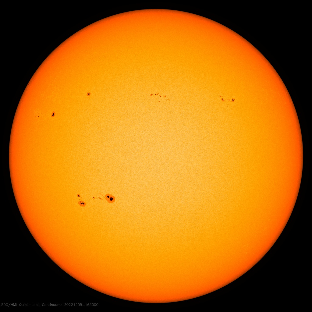
(a) Full surface of the Sun, sunspots are the regions that appear darker than the continuum. The solar surface appears darker on the limb, a fact known as the limb-darkening effect.

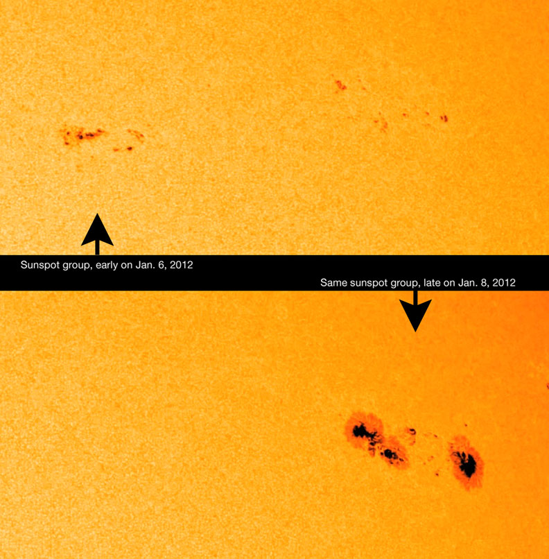
(b) Same group of sunspots observed at two different dates, top: Jan 6 2012, bottom: Jan 8 2012.The granular aspect of the continuum comes from the convective motion of the gas at the stellar surface.

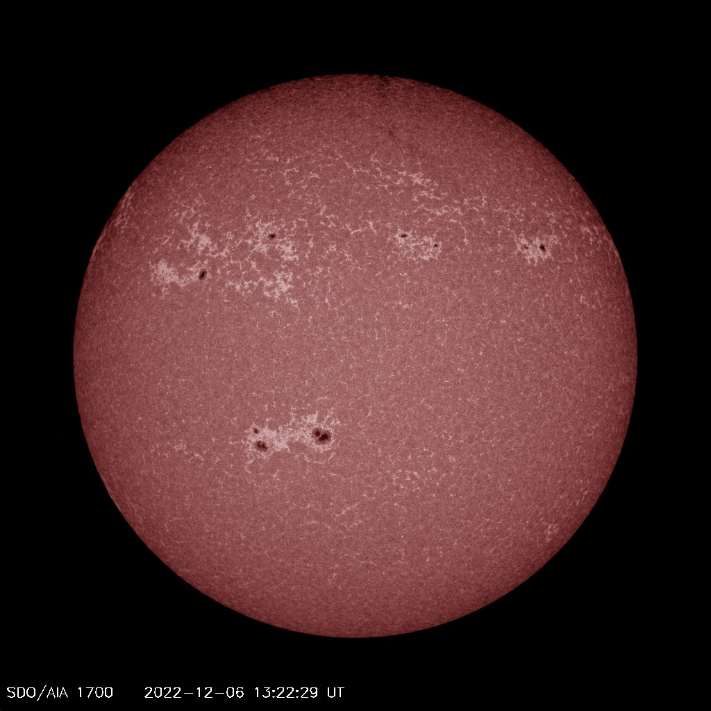
(c) SDO observation of the Sun at wavelength 1700 Å. The bright regions are called faculae, notice that faculae areas surround the spots (darker regions). Both faculae and spots inhibit the upward convective motion of the gas. Faculae cover more area than spots, but have a smaller temperature contrast with the continuum. The latitude, number and lifetime of the spots varies along stellar magnetic cycles, on the timescale of a few years (11 years for the Sun).

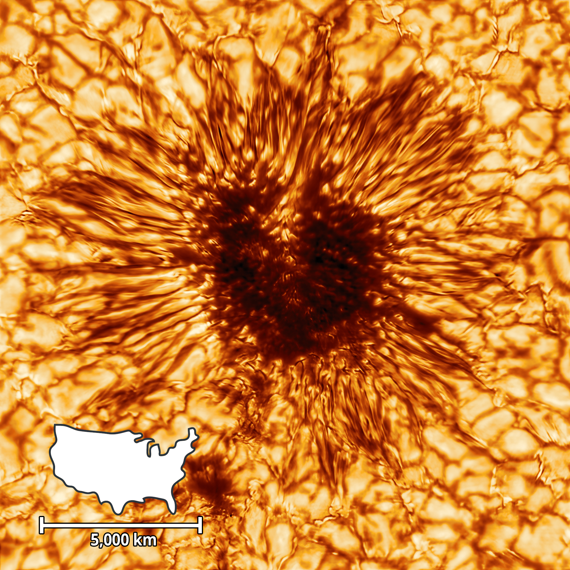
(d) Inouye Solar Wave Front Correction (WFC) image, captured Jan 28, 2020, at 530 nanometers. The granulated structures around the spot are due to convection: hot plasma moves upwards at the center of granules, cools down and goes downwards between granules (darker inter-granular regions). The contribution of brighter intra-granular region exceeds that of intergranular ones, creating a so-called convective bluedhift on observed spectra. Credit: NSO/AURA/NSF

Figure 8: Solar dynamics observatory (SDO) images of the Sun in filtered light. Figures in (a), (b), and (c) are courtesy of NASA/SDO and the AIA, EVE, and HMI science teams.

Understanding the impact of the variability of stellar surfaces on the signal is important to reach a precision below 1 m/s. There are several types of effects on stellar surface which affect the spectra measured and imprint onto the estimated radial velocities.

The physical processes taking place in stellar surfaces, how they vary depending on the type of star, and their impact on the data have been investigated through simulations, observations of the Sun and other stars. For a review of stellar effects affecting the RV, we refer the reader to Cegla (2019), Meunier (2021).

Stars can be locally brighter and darker because of local excess magnetic field (see Fig. 8). As the observed star rotates, the feature breaks the imbalance between the approaching and receding stellar limbs, respectively blue-shifted and red-shifted. Furthermore, these structures inhibit the upwards convective motion of the gas, an effect known as the convective blueshift inhibition (Dravins et al., 1981). The effect of these magnetic structures on the radial velocity and activity indicators has been simulated for Sun-like stars in Saar & Donahue (1997), Hatzes (2002), Desort et al. (2007), Boisse et al. (2012), Dumusque et al. (2014), Borgniet et al. (2015), Dumusque (2016), Meunier et al. (2019), Bellotti & Korhonen (2021), and for M dwarves in Barnes et al. (2011). Simulations can also be used directly to forward-model and analyse the data (Herrero et al., 2016). The apparition of spots varies through the stellar magnetic cycle on the scale of $\sim$ 10 years, creating signals at this timescale (Makarov, 2010, Meunier & Lagrange, 2013, Fuhrmeister et al., 2022).

Convection on the surface of the star creates a so-called granulation pattern (see Fig. 8(d), and Cegla (2019) for a review). The effect of the changing patterns of convection on radial velocity and indicators changes with stellar spectral types (Meunier et al., 2017) and has been simulated in several works, Cegla et al. (2013), Meunier et al. (2015), Cegla et al. (2018), Dravins et al. (2021). In simulations, the effect of this process on RV appears to be correlated to its effect on activity indicators (Meunier & Lagrange, 2013, Cegla et al., 2019), a fact that is still to be fully leveraged for the correction of the RV granulation effect.

Stellar variability models need to be calibrated. This was initially done through the observation with the HARPS spectrograph of the solar light scattered by the asteroid 4/Vesta, with simultaneous high resolution observations of the solar surface with the solar dynamics observatory (SDO). From the surface observations, and based on the physical understanding of RV effect, the expected RV is computed and compared to the HARPS RV measurements (Haywood et al., 2016). The lifetime and properties of granules on the Sun can be also derived from observations of the Sun (e.g. Hirzberger et al., 1999). An interesting observation is that, even though the lifetime of granules is $\sim 15$ min, averaging the solar surface for 1h does not completely average out their effect. Furthermore, in recent years, several telescopes were built to observe the Sun and feed high precision spectrographs used to detect exoplanets at night. Such telescopes exist for HARPS-N (Dumusque et al., 2015, Phillips et al., 2016), HARPS and NIRPS spectrograph, NEID (Lin et al., 2022), EXPRES (Llama et al., 2022), and Keck Planet Finder (KPF) . Several years of high-resolution solar spectra are publically avaliable from HARPS-N (Dumusque et al., 2021) and NEID . And astronomers are beginning to draw conclusions about the Sun’s variability based on Sun-as-a-star observations (e.g., Collier Cameron et al., 2019, Miklos et al., 2020, Al Moulla et al., 2022b)

Another well explored area consists in studying the spectroscopic observations of other stars, in particular the radial velocities and activity indicators. There has been substantial work on the observation of M dwarves (e. g. Bonfils et al., 2007, Forveille et al., 2009, Suárez Mascareño et al., 2018, Zechmeister et al., 2018, Jeffers et al., 2022), in particular the periods of the exhibited variability, using the CARMENES sample (Schöfer et al., 2019, Lafarga et al., 2020, Schöfer et al., 2022). It was shown in particular that some activity indicators exhibit a closed-loop pattern. It means that when plotting the time series of RV acquired at times $t_{i},i=1,...,N$ not against time, but as a function of an activity indicator at time $t_{i}$, the figure exibits a loop pattern. The behaviour of the indicators in Sun-like stars has been studied in Gomes da Silva et al. (2011), Boisse et al. (2011), Gomes da Silva et al. (2012), Figueira et al. (2013), Santerne et al. (2015), Lanza et al. (2018), Suárez Mascareño et al. (2020). The effect of granulation on RV and photometry has been studied in Sulis et al. (2022) with simultaneous CHEOPS and ESPRESSO observations of two stars, of spectral type G and F.

More recently, attention has been given to the color-dependent effect of stellar activity: depending on their wavelength, spectral lines are affected differently (Thompson et al., 2017, Wise et al., 2018, Cretignier et al., 2020a, Ning et al., 2019, Wise et al., 2022, Al Moulla et al., 2022a, Lafarga et al., 2023). This aspect will be crucial to leverage all the information present in the spectrum to estimate the contaminating signal in RVs (see Eq. (18)). This knowledge might be coupled to data-driven approach leveraging all the spetral information (Bedell et al., 2019, Gully-Santiago & Morley, 2022, Gilbertson & Ford, 2022).

In addition to magnetic activity and granulation, acoustic oscillations of the stars also affect the data (Dumusque et al., 2011b, Chaplin et al., 2019, Guo et al., 2022). The most important oscillations for solar-type stars (known as $p$ modes) have characteristic periods of a few to several minutes. Stellar Meridional winds (Beckers, 2007, Makarov, 2010), as well as gravitational redshift (Cegla et al., 2012) also affect the data at the level of a few cm/s.

To conclude this section, let us note that the problem laid out in §A has some similarities with the setting of a technique called Doppler imaging, which relies on the following principle. As we have seen above, the presence of magnetically active region on the surface of the star changes the shape of the spectral lines. Conversely, one can infer the position and size of magnetic regions from the change of shape of the spectrum (for stars that rotate sufficiently fast). The inference is usually done on a weighted average of the spectral lines (Khokhlova, 1976, Goncharskii et al., 1977, 1982, Vogt & Penrod, 1983, Vogt et al., 1987). From spectrapolarimetric observations, one can also retrieve some properties of the magnetic field (Donati et al., 1997). In §A, we do not aim at retrieving the distribution of stellar spots from a shape change in the spectrum, but at estimating the contaminating RV signal. Another approach consists of estimating the distribution of stellar spots with a Doppler imaging approach, and predicting the corresponding RV signal Lanza et al. (2011), Petit et al. (2015), Barnes et al. (2017), Yu et al. (2019), Klein et al. (2022), see Barnes et al. (2015, 2017), Hébrard et al. (2016), Baroch et al. (2020) for the particular case of M dwarves. While this can work well for stars with one or two large active regions, the problem becomes underconstrained once one allows for several active regions being active at once and/or smaller active regions that evolve on shorter timescales. Luger et al. (2021a) builds explicitly a likelihood for the Doppler imaging problem and provides a framework for marginalizing over surface maps. While this can work well for stars with large active regions, applying it to active regions more typical of sun-like stars has yet to be proven practical, as it would require a very high-order spherical harmonic expansion of the solar surface.

Appendix C PERIODOGRAMS

Let us suppose we have a timeseries with $N$ entries, $\mathbf{y}=(y(t_{i}))_{i=1,..N}$. We want to determine if $\mathbf{y}$ exhibits periodic variations, here potentially due to planets. A common way to do this is to use a family of methods called periodograms. Such methods consist in computing the difference of log-likelihoods of a null hypothesis model $H_{0}$ and an alternative model $K_{\omega}$, including $H_{0}$ and one or several periodic signals. The simplest form of periodogram is the Lomb-Scargle periodogram (Lomb, 1976, Scargle, 1982). With the notations of Eq. (21) the alternative models are both Gaussian multivariate distributions such that

$$H_{0}:\; \mathbf{g}=\mathbf{0},$$ (27)

$$K_{\omega}:\; \mathbf{g}(A,B,\omega)=A\cos\omega\mathbf{t}+B\sin\omega\mathbf{t},$$ (28)

where $A$ and $B$ are chosen to maximize the log likelihood of $K_{\omega}$, which is here equivalent to finding $A$ and $B$ minimizing the sum of squares $\sum_{i=1}^{N}(y(t_{i})-A\cos\omega(t_{i})-B\sin\omega(t_{i}))^{2}/\sigma_{i}^{2}$, where $\sigma_{i}$ is the error on measurement $i$. The null hypothesis expresses how the data is expected to behave in the absence of periodic components. For the Lomb-Scargle periodogram, the null hypothesis is that the data is a realization of a Gaussian, uncorrelated noise.

In general, denoting by $\bm{\mathord{\mkern 1.3mu\ThisStyle{\mbox{\hskip 13.76387pt{1 0 -.25 1}\hbox to0.0pt{\hss\leavevmode\hbox{$\SavedStyle\theta$}}}}\mkern-1.3mu}}_{K}$ and $\bm{\mathord{\mkern 1.3mu\ThisStyle{\mbox{\hskip 13.76387pt{1 0 -.25 1}\hbox to0.0pt{\hss\leavevmode\hbox{$\SavedStyle\theta$}}}}\mkern-1.3mu}}_{H}$ the parameters of models $K_{\omega}$ and $H_{0}$, the periodogram of time series $\mathbf{y}$ evaluated in frequency $\omega$ is

$$\mathcal{P}(\omega)=\max_{\bm{\mathord{\mkern 1.3mu\ThisStyle{\mbox{\hskip 9.6347pt{1 0 -.25 1}\hbox to0.0pt{\hss\leavevmode\hbox{$\SavedStyle\theta$}}}}\mkern-1.3mu}}_{K_{\omega}}}\log p(\mathbf{y}\mid\bm{\mathord{\mkern 1.3mu\ThisStyle{\mbox{\hskip 13.76387pt{1 0 -.25 1}\hbox to0.0pt{\hss\leavevmode\hbox{$\SavedStyle\theta$}}}}\mkern-1.3mu}}_{K_{\omega}})-\max_{\bm{\mathord{\mkern 1.3mu\ThisStyle{\mbox{\hskip 9.6347pt{1 0 -.25 1}\hbox to0.0pt{\hss\leavevmode\hbox{$\SavedStyle\theta$}}}}\mkern-1.3mu}}_{H_{0}}}\log p(\mathbf{y}\mid\bm{\mathord{\mkern 1.3mu\ThisStyle{\mbox{\hskip 13.76387pt{1 0 -.25 1}\hbox to0.0pt{\hss\leavevmode\hbox{$\SavedStyle\theta$}}}}\mkern-1.3mu}}_{H_{0}})$$ (29)

Other definitions are possible, in particular some authors normalize the periodogram by $\max_{\bm{\mathord{\mkern 1.3mu\ThisStyle{\mbox{\hskip 9.6347pt{1 0 -.25 1}\hbox to0.0pt{\hss\leavevmode\hbox{$\SavedStyle\theta$}}}}\mkern-1.3mu}}_{H_{0}}}\log p(\mathbf{y}\mid\bm{\mathord{\mkern 1.3mu\ThisStyle{\mbox{\hskip 13.76387pt{1 0 -.25 1}\hbox to0.0pt{\hss\leavevmode\hbox{$\SavedStyle\theta$}}}}\mkern-1.3mu}}_{H_{0}})$ (Baluev, 2008). The periodogram is computed on a grid of frequencies, $\Omega=(\omega_{i})_{i=1..N}$. We compute the maximum of the periodogram of the data to be analysed $\mathbf{y}$, which we denote by $\mathcal{P}_{\mathrm{d}}$, and define a false alarm probability,

$$p(\max_{\omega\in\Omega}\mathcal{P}(\omega)\geqslant\mathcal{P}_{\mathrm{d}}\mid H_{0})$$ (30)

that is the probability that the maximum of the periodogram exceeds $\mathcal{P}_{\mathrm{d}}$ knowing $H_{0}$ is true. A small FAP means the hypothesis $H_{0}$ is unlikely. If one generates $M$ signals following the hypothesis $H_{0}$ and computes their periodogram, the FAP is simply the number of times the maximum of the periodogram exceeds $\mathcal{P}_{d}$ divided by $M$. This brute force approach gives a precision of 100/$M$ % on the FAP. To evaluate whether the FAP is below 0.01 % requires at least 10,000 simulations. However, thanks to the theory of extreme values of stochastic process, it is possible to obtain analytical approximations of the FAP associated to a certain definition of the periodograms, which greatly facilitates the use of periodograms (Baluev, 2008, 2009, 2013, 2013a, 2015b, Delisle et al., 2020a). In the following, we will make explicit whether such a formula exists. In between the brute force and analytical approaches, the method of Süveges (2014) consists in generating a few datasets following the null hypothesis, and fit to the cumulative distribution function of maxima of the periodograms a generalised extreme value (GEV) distribution.

The periodogram has been extended to definitions of the likelihoods of $H_{0}$ and $K_{\omega}$ more complex than the Lomb-Scargle periodogram.The models are often assumed to be Gaussian, and each have a likelihood in the form of (21) In Ferraz-Mello (1981), Cumming et al. (1999), Reegen (2007), Zechmeister & Kürster (2009) the Lomb-Scargle periodogram is generalized by fitting for $c_{0}$, as defined in Eq. (22) at each trial period. Ford (2008) extends the definition of $H_{0}$ to $c_{0}\mathbf{1}+c_{1}\mathbf{t}$ where $\mathbf{t}=(t_{i})_{i=1..N}$. These are particular instances of the case considered in Baluev (2008), where $H_{0}$ is a linear model $\mathbf{M}\mathbf{x}$, $\mathbf{M}$ is a $N\times p$ matrix and $\mathbf{x}$ a vector of size $p$,

$$H_{0}:\; \mathbf{g}(\mathbf{x})=\mathbf{M}\mathbf{x},$$ (31)

$$K_{\omega}:\; \mathbf{g}(A,B,\omega,\mathbf{x})=\mathbf{M}\mathbf{x}+A\cos\omega\mathbf{t}+B\sin\omega\mathbf{t},$$ (32)

where $\mathbf{x},A$ and $B$ are fitted for each trial frequency to maximize the likelihood of model $K_{\omega}$. This framework can be applied to fitting separate offsets $c_{0}$ for each instrument. If there are $p$ instruments, one simply has to define $\mathbf{M}_{ij}=1$ if measurement at time $t_{i}$ is taken by instrument $j$, and $\mathbf{M}_{ij}=0$ otherwise. This framework also allows to approximately compare $n+1$ vs. $n$ planets instead of 1 vs. 0, when including in the columns of $\mathbf{M}$ the $\cos\omega_{i}\mathbf{t}$ and $\sin\omega_{i}\mathbf{t}$ of the frequencies of planets found so far $\omega_{i}$, $i=1,..,n$. Baluev (2008) provides an accurate analytical false alarm probability.

So far, $\mathbf{V}$ is supposed fixed. The noise model can also be generalized by allowing for an unknown $\sigma_{J}$ fitted at each frequency (Baluev, 2009). Here, the noise is still assumed to be uncorrelated temporally, which is unrealistic in many cases due to the presence of stellar activity and instrumental systematics. The analytical FAP formula is generalised in Delisle et al. (2020a) to arbitrary, fixed covariance matrix $\mathbf{V}$, thus generalising the formula of Sulis et al. (2016) to the case of uneven sampling and non stationary Gaussian noises. It is also possible to fit the parameters of a non white noise model at each trial frequency, but this is costly and there is no analytical formula for the FAP (Delisle et al., 2018).

Another line of work generalizes the form of the periodic function. Instead of fitting a sinusoid, the $K_{\omega}$ model can be defined as a Keplerian model (Cumming, 2004, Zechmeister & Kürster, 2009). This is particularly useful to detect signals of planets with high orbital eccentricity. Baluev (2015b) provides a rigorous analytical FAP in that case, as a special case of analytical FAPs for non-sinusoidal signals Baluev (2013a).

Furthermore, instead of searching for one periodicity, it is possible to search for multiple planets simultaneously (Ford et al., 2011, Baluev, 2013), and jointly modeling RVs and other stellar ancillary indicators (Delisle et al., 2022, Jones et al., 2022).

Instead of computing the maximum likelihood models for $H_{0}$ and $K_{\omega}$, one can marginalize over certain parameters. It means that instead of maximizing $p(\mathbf{y}\mid\bm{\mathord{\mkern 1.3mu\ThisStyle{\mbox{\hskip 13.76387pt{1 0 -.25 1}\hbox to0.0pt{\hss\leavevmode\hbox{$\SavedStyle\theta$}}}}\mkern-1.3mu}}_{K_{\omega}})$ over $\bm{\mathord{\mkern 1.3mu\ThisStyle{\mbox{\hskip 13.76387pt{1 0 -.25 1}\hbox to0.0pt{\hss\leavevmode\hbox{$\SavedStyle\theta$}}}}\mkern-1.3mu}}_{K_{\omega}}$, we separate the parameters in two categories $\bm{\mathord{\mkern 1.3mu\ThisStyle{\mbox{\hskip 13.76387pt{1 0 -.25 1}\hbox to0.0pt{\hss\leavevmode\hbox{$\SavedStyle\theta$}}}}\mkern-1.3mu}}_{K_{\omega}}=(\bm{\mathord{\mkern 1.3mu\ThisStyle{\mbox{\hskip 13.76387pt{1 0 -.25 1}\hbox to0.0pt{\hss\leavevmode\hbox{$\SavedStyle\theta$}}}}\mkern-1.3mu}}_{K_{\omega}}^{1},\bm{\mathord{\mkern 1.3mu\ThisStyle{\mbox{\hskip 13.76387pt{1 0 -.25 1}\hbox to0.0pt{\hss\leavevmode\hbox{$\SavedStyle\theta$}}}}\mkern-1.3mu}}^{2})$, $\bm{\mathord{\mkern 1.3mu\ThisStyle{\mbox{\hskip 13.76387pt{1 0 -.25 1}\hbox to0.0pt{\hss\leavevmode\hbox{$\SavedStyle\theta$}}}}\mkern-1.3mu}}_{H_{0}}=(\bm{\mathord{\mkern 1.3mu\ThisStyle{\mbox{\hskip 13.76387pt{1 0 -.25 1}\hbox to0.0pt{\hss\leavevmode\hbox{$\SavedStyle\theta$}}}}\mkern-1.3mu}}_{H_{0}}^{1},\bm{\mathord{\mkern 1.3mu\ThisStyle{\mbox{\hskip 13.76387pt{1 0 -.25 1}\hbox to0.0pt{\hss\leavevmode\hbox{$\SavedStyle\theta$}}}}\mkern-1.3mu}}^{2})$, and compute

$$p(\mathbf{y}\mid\bm{\mathord{\mkern 1.3mu\ThisStyle{\mbox{\hskip 13.76387pt{1 0 -.25 1}\hbox to0.0pt{\hss\leavevmode\hbox{$\SavedStyle\theta$}}}}\mkern-1.3mu}}_{K_{\omega}}^{1})=\int p(\mathbf{y}\mid\bm{\mathord{\mkern 1.3mu\ThisStyle{\mbox{\hskip 13.76387pt{1 0 -.25 1}\hbox to0.0pt{\hss\leavevmode\hbox{$\SavedStyle\theta$}}}}\mkern-1.3mu}}_{K_{\omega}}^{1},\bm{\mathord{\mkern 1.3mu\ThisStyle{\mbox{\hskip 13.76387pt{1 0 -.25 1}\hbox to0.0pt{\hss\leavevmode\hbox{$\SavedStyle\theta$}}}}\mkern-1.3mu}}^{2})p(\bm{\mathord{\mkern 1.3mu\ThisStyle{\mbox{\hskip 13.76387pt{1 0 -.25 1}\hbox to0.0pt{\hss\leavevmode\hbox{$\SavedStyle\theta$}}}}\mkern-1.3mu}}^{2})\operatorname{d}\bm{\mathord{\mkern 1.3mu\ThisStyle{\mbox{\hskip 13.76387pt{1 0 -.25 1}\hbox to0.0pt{\hss\leavevmode\hbox{$\SavedStyle\theta$}}}}\mkern-1.3mu}}^{2}\;\;;\;\;p(\mathbf{y}\mid\bm{\mathord{\mkern 1.3mu\ThisStyle{\mbox{\hskip 13.76387pt{1 0 -.25 1}\hbox to0.0pt{\hss\leavevmode\hbox{$\SavedStyle\theta$}}}}\mkern-1.3mu}}_{H_{0}}^{1})=\int p(\mathbf{y}\mid\bm{\mathord{\mkern 1.3mu\ThisStyle{\mbox{\hskip 13.76387pt{1 0 -.25 1}\hbox to0.0pt{\hss\leavevmode\hbox{$\SavedStyle\theta$}}}}\mkern-1.3mu}}_{H_{0}}^{1},\bm{\mathord{\mkern 1.3mu\ThisStyle{\mbox{\hskip 13.76387pt{1 0 -.25 1}\hbox to0.0pt{\hss\leavevmode\hbox{$\SavedStyle\theta$}}}}\mkern-1.3mu}}^{2})p(\bm{\mathord{\mkern 1.3mu\ThisStyle{\mbox{\hskip 13.76387pt{1 0 -.25 1}\hbox to0.0pt{\hss\leavevmode\hbox{$\SavedStyle\theta$}}}}\mkern-1.3mu}}^{2})\operatorname{d}\bm{\mathord{\mkern 1.3mu\ThisStyle{\mbox{\hskip 13.76387pt{1 0 -.25 1}\hbox to0.0pt{\hss\leavevmode\hbox{$\SavedStyle\theta$}}}}\mkern-1.3mu}}^{2}$$ (33)

Typically $\bm{\mathord{\mkern 1.3mu\ThisStyle{\mbox{\hskip 13.76387pt{1 0 -.25 1}\hbox to0.0pt{\hss\leavevmode\hbox{$\SavedStyle\theta$}}}}\mkern-1.3mu}}_{K_{\omega}}^{1}$ is the frequency and $\bm{\mathord{\mkern 1.3mu\ThisStyle{\mbox{\hskip 13.76387pt{1 0 -.25 1}\hbox to0.0pt{\hss\leavevmode\hbox{$\SavedStyle\theta$}}}}\mkern-1.3mu}}^{2}$ are parameters on which the model depends linearly. In that case, marginalization can be done with analytical expressions (Cumming, 2004, Mortier et al., 2015, Feng et al., 2017). Marginalizing can also be done via the Laplace approximation (Ford, 2008, Nelson et al., 2020) or by using numerical quadrature. The latter method has been used to marginalize over a noise term $\sigma_{J}$ at each trial frequency (Nelson et al., 2020, Appendix A3). Conceptual and practical differences between using the maximization or marginalization of the likelihood are discussed in Baluev (2022).

The type of periodogram to use depends on the trade-off between precision and speed needed. The availability of an accurate analytical FAP is the major driver of the speed, since there is no need to compute periodograms several times. Analytical estimates listed above are reliable for signals with a FAP of 0.1 or lower. All periodograms involving a linear fit with an analytical FAP (Baluev, 2008, Delisle et al., 2020a) are very fast (a few seconds on a typical dataset, on a laptop). Keplerian or multi frequency periodograms can take longer (several minutes at least).

Appendix D BAYESIAN MODEL COMPARISON: COMPUTATIONAL CHALLENGES

Bayesian model comparison involves computing the Bayesian evidence, of marginal likelihood. The Bayesian of evidence (also called marginal likelihood) of a $n$ planet model is

$$p(\mathbf{y}\mid n)=\iint_{\Theta_{n}}p(\mathbf{y}\mid\bm{\mathord{\mkern 1.3mu\ThisStyle{\mbox{\hskip 13.76387pt{1 0 -.25 1}\hbox to0.0pt{\hss\leavevmode\hbox{$\SavedStyle\theta$}}}}\mkern-1.3mu}},\bm{\mathord{\mkern 1.3mu\ThisStyle{\mbox{\hskip 14.03473pt{1 0 -.25 1}\hbox to0.0pt{\hss\leavevmode\hbox{$\SavedStyle\eta$}}}}\mkern-1.3mu}},n)p(\bm{\mathord{\mkern 1.3mu\ThisStyle{\mbox{\hskip 13.76387pt{1 0 -.25 1}\hbox to0.0pt{\hss\leavevmode\hbox{$\SavedStyle\theta$}}}}\mkern-1.3mu}},\bm{\mathord{\mkern 1.3mu\ThisStyle{\mbox{\hskip 14.03473pt{1 0 -.25 1}\hbox to0.0pt{\hss\leavevmode\hbox{$\SavedStyle\eta$}}}}\mkern-1.3mu}}\mid n)\operatorname{d}\bm{\mathord{\mkern 1.3mu\ThisStyle{\mbox{\hskip 13.76387pt{1 0 -.25 1}\hbox to0.0pt{\hss\leavevmode\hbox{$\SavedStyle\theta$}}}}\mkern-1.3mu}}\operatorname{d}\bm{\mathord{\mkern 1.3mu\ThisStyle{\mbox{\hskip 14.03473pt{1 0 -.25 1}\hbox to0.0pt{\hss\leavevmode\hbox{$\SavedStyle\eta$}}}}\mkern-1.3mu}}.$$ (34)

and the ratio $p(\mathbf{y}\mid n+1)/p(\mathbf{y}\mid n)$, referred to as a Bayes factor, is a very common statistical significance metric for exoplanet detection. If $n$ planets have been confidently detected, and if the Bayes factor is above a certain threshold, the detection of the $n+1$th planet is claimed. The computation of the evidence and a reliable estimation of the posterior distribution $p(\bm{\mathord{\mkern 1.3mu\ThisStyle{\mbox{\hskip 13.76387pt{1 0 -.25 1}\hbox to0.0pt{\hss\leavevmode\hbox{$\SavedStyle\theta$}}}}\mkern-1.3mu}},\bm{\mathord{\mkern 1.3mu\ThisStyle{\mbox{\hskip 14.03473pt{1 0 -.25 1}\hbox to0.0pt{\hss\leavevmode\hbox{$\SavedStyle\eta$}}}}\mkern-1.3mu}}\mid\mathbf{y},n)$ are both crucial for a useful Bayesian detection criteria that results in the posterior probability for a planet to be within a confined region of the parameter space (Brewer & Donovan, 2015, Faria et al., 2022, Hara et al., 2022c).

Evaluating an integral over a large parameter space is notoriously difficult. One of the difficulties of radial velocity data is that the model contains periodic signals. The frequency resolution is approximately 2$\pi/T_{\mathrm{obs}}$ where $T_{\mathrm{obs}}$ is the total timespan of observation. As a result, in a frequency range $[\omega_{1},\omega_{2}]$ with $\Omega=\omega_{2}-\omega_{1}$, the number of local likelihood maxima is approximately $N_{\mathrm{locmax}}=\Omega T_{\mathrm{obs}}/2\pi$. If there are $k$ periodic signals with frequencies in the same range, we should expect $\sim N_{\mathrm{locmax}}^{k}$ local minima when varying the frequencies. Furthermore, the geometry of the Keplerian signals is such that there are many local minima at high eccentricity (Baluev, 2015b, Hara et al., 2019).

To compute Eq. (34), two family of methods are used: Monte-Carlo Markov Chain (MCMC) and nested sampling. In both cases, special attention must be paid to the exploration of the complex parameter space. MCMC methods rely on the definition of a proposal distribution, which must lead to samples both jumping from local minima far from each other, and explore the dominant modes. The numerical difficulty of nested sampling algorithms is to find efficiently a sequence of independent samples following the prior distribution restricted to regions of the parameter space with sufficient likelihood.

Ford & Gregory (2007) compared several methods for estimating the Bayesian evidence, and found that several performed particularly poorly for our standard model. Methods that performed well for the 1-planet model were: the Laplace approximation, importance sampling, the “ratio estimator” (Nelson et al., 2016), and parallel tempering Monte-Carlo Markov Chain (MCMC) (Gregory, 2007b). Subsequently, several authors have applied nested sampling algorithms (Brewer, 2014, Handley et al., 2015b, Faria et al., 2016, Buchner, 2021), which couple the estimation of the posterior distribution with the Bayesian evidence (Eq. 34).

In order to better understand the strengths and limitations of approaches for computing Bayesian evidences, Nelson et al. (2020) designed a data challenge in coordination with the 3rd Extreme Precision Radial Velocity workshop (Penn state, August 14-17 2017). Nine participants/teams were given two sets of priors, and four likelihoods (corresponding to 0, 1, 2 and 3-planet models) and 6 simulated datasets. Teams compared their results for the first dataset during the workshop, refined their methods and submitted updated results. Collectively, teams reported estimates of the marginalized likelihood and its uncertainty using fifteen computational methods.

As expected, some methods (e.g., Bayes Information Criterion, Chib’s estimator) gave highly discrepant results for Bayes factors. Laplace approximation typically agreed with other high-quality methods to within a factor of $\sim~{}10^{2}$ for 0 to 2-planet models and $\sim~{}10^{4}$ for a 3-planet model. Of the remaining methods, there was general agreement for the Bayes factor to within a factor of $\sim~{}10$ for 1-planet models, and $\sim~{}10^{2}$ for 2 and 3-planet models. Methods that demonstrated broad agreement included: combining MCMC with importance sampling using either the Perrakis estimator (Perrakis et al., 2014) or the ratio estimator (Nelson et al., 2016), variational Bayes with importance sampling (Beaujean & Caldwell, 2013), and multiple forms of nested sampling (Veitch & Vecchio, 2010, Feroz et al., 2009, Feroz & Skilling, 2013). It is unclear why diffusive nested sampling (using DNest4; Brewer, 2016) sometimes gave results significantly discrepant from the other Bayesian methods.

The significant dispersion in numerical estimates of Bayes factors emphasizes the importance of adopting a threshold Bayes factor much larger than is typically recommended in the literature (often 150, in the context of much simpler models). At first, it may seem concerning that different estimates of Bayes factors could vary by a few orders of magnitude. In practice, Bayes factors for RV datasets are often so extreme that an uncertainty of “only” a few orders of magnitude is acceptable. Of course, publication biases can result in planet discoveries being preferentially reported when the Bayes factor is still “only” a few to several of orders of magnitude from unity.

Another important result of this data challenge was that the observed dispersion of Bayes factors estimates was often significantly greater than predicted for some methods. Therefore, when using iterative algorithms, it is important to compute and report uncertainties for Bayes factors based on multiple independent runs.

Appendix E MODEL: SPECIFYING THE PRIORS AND LIKELIHOODS

E.1 Priors

The choice of priors affects both orbital parameter estimates and model comparison to determine the number of planets, especially for low amplitude signals, where the likelihood is flatter (Hara et al., 2022c). Based on a combination of astrophysical and statistical considerations, Ford & Gregory (2007) recommend the following priors: $p(\log P)\sim U[\log P_{\mathrm{min}},\log P_{\mathrm{max}}]$ $p(e)\sim U[0,1)$, $p(\omega)\sim U[0,2\pi)$, $p(M_{0})\sim U[0,2\pi)$, and $p(c_{0})\sim U[-c_{0,\mathrm{max}},c_{0,\mathrm{max}}]$, where $U$ represents a uniform prior with the given bounds. For minimally informed priors of scale variables, Ford & Gregory (2007) introduce a prior distribution for a real variable $z\in[0,z_{\mathrm{max}}]$, defining $0<z_{0},z_{\mathrm{max}}$

$$p_{FG}(z\mid z_{o},z_{\mathrm{max}})=\frac{(z_{o}+z)^{-1}}{\log(1+z_{\mathrm{max}}/z_{o})},$$ (35)

they recommend $p(K\mid P)\sim p_{FG}(K\mid K_{o},K_{\mathrm{max}}(P_{\mathrm{min}}/P)^{1/3})$ and $p(\sigma_{J})\sim p_{FG}(\sigma_{J}\mid\sigma_{J,o},K_{\mathrm{max}})$. Physically motivated choices for $P_{\mathrm{min}}$ and $K_{\mathrm{max}}$ vary with the target star properties. For instance, the values of $K$ and $P$ corresponding to a planet that would be disintegrated with tidal forces, that is beyond the Roche limit, are excluded. Typical values for a sun-like star would be $P_{\mathrm{min}}=0.2$ days and $K_{\mathrm{max}}=3.6$ km/s. Non-zero values of $K_{o}$ and $\sigma_{J,o}$ are necessary to ensure proper priors. Ford & Gregory (2007) recommend $K_{o}=\sigma_{J,o}=\sigma_{\mathrm{RV},o}\sqrt{50/N_{\mathrm{obs}}}$, where $\sigma_{\mathrm{RV},o}$ is the typical measurement precision and $N_{\mathrm{obs}}$ is the number of observations, so as to provide sensitivity to planets within the realm of detection without overly penalizing models for planets that are essentially impossible to detect with available data. Posterior distributions for $e$ and $\omega$ vary considerably with the quality of the data. As geometric considerations dictate the prior for $\omega$, the only priors that are likely to affect the estimation of orbital parameters are those of $K$ and $e$.

Table 1: Reference Priors

Parameter	Variable	Unit	Distribution	Note
Orbital Period	$P$	d	$\log P\sim U[\log P_{\min},\log P_{\max}]$	$a,b$
Velocity Amplitude	$K$	m s-1	$\log K\sim p_{FG}(K_{o},K_{\max}\left(\frac{P_{\min}}{P}\right)^{1/3})$	$c,d$
Orbital Eccentricity	$e$	…	$e\sim U[0,e_{\max}(P))$	$e$
Argument of Pericenter	$\omega$	radians	$\omega\sim U[0,2\pi)$	f
Mean Anomaly at epoch	$M_{0}$	radians	$M_{0}\sim U[0,2\pi)$	f
RV offset	$c_{0}$	m s-1	$c_{0}\sim N[0,\sigma^{2}_{\mathrm{disp}}]$	g
RV slope	$c_{1}$	m s-1 yr-1	$c_{1}\sim N[0,\sigma^{2}_{c_{1}}]$	h

^a For sun-like stars, astrophysical considerations justify hard limits of $P_{\min}\simeq~{}0.2$d and $P_{\max}\simeq~{}10^{8}$ year. However, theory predicts that the occurrence rate drops dramatically at much shorter orbital periods ($\simeq~{}1000^{3}$yr). In practice, RV surveys are limited by the survey duration and the choice of $P_{\max}$ is only important when performing model comparison. ^b Empirically, the planet occurrence rate decreases for periods less than $3$d. For an analytical reference prior that limits how much very-short period planets are overweighted relative to nature, one might adopt $P\sim p_{FG}(3\mathrm{d},P_{\max})$, truncate assign no probability to periods less than $P_{\min}$. ^c The intrinsic occurrence rate of small planets may to continue rising to smaller amplitudes than are typically detectable for the foreseeable future. In practice, we recommend setting $K_{o}=\sigma_{RV,1\mathrm{obs}}\sqrt{50/N_{\mathrm{obs}}}$, so as to reflect the limiting precision of an RV survey, where $\sigma_{RV,1\mathrm{obs}}$ is measurement precision of a single observations and $N_{\mathrm{obs}}$ is the number of observations. Since there will not be strong evidence for a planet with $K$ less than the detection limit of a survey, there is no benefit to assigning substantial prior mass to such planets. ^d For Sun-like stars and $P_{\min}=0.2$d, $K_{\max}\simeq~{}3.6$km/s. Larger RV signals would be due to perturbations by a stellar binary companion, rather than an exoplanet. ^e Keplerian orbital models develop pathologically narrow spikes for $e\simeq~{}1$. Formally, one could avoid these by imposing a maximum eccentricity, $e_{\max}(P)=1-\left(\frac{r_{p,\min}}{AU}\right)\left(\frac{P}{\mathrm{yr}}\right)^{-2/3}\left(\frac{M_{\star}}{M_{\odot}}\right)^{-1/3}$, so as to ensure the planet’s pericenter distance exceeds the Roche limit, $r_{p,\min}$. In practice, most MCMC and nested samplers do not find the pathological solutions for $e\simeq~{}1$ and thus practioners set $e_{\max}=1$, but ignore the contributions from $e\simeq~{}1$ solutions. Kipping (2014) uses a beta prior fitted on the eccentricity of known giant planets, which disfavours high eccentricities. ^f Geometric considerations provide a strong motivation for this choice. ^g For surveys of sun-like stars in the solar neighborhood, a dispersion of $\sigma_{\mathrm{disp}}\simeq~{}40$km s^-1 would be well-motivated by knowledge of Milky Way structure. While astrophysical knowledge could motivate alternative choices for other populations, in practice this has minimal effect as long as the prior assigns non-zero mass to the true mean radial velocity offset. In practice, most practitioners assign a uniform prior. ^h $\sigma_{c_{1}}\simeq~{}10$ km s^-1 is representative of the acceleration due to a wide binary companion. The specific choice of prior is unlikely to effect parameters for any well-characterized planets once the timespan of observations exceeds two orbital periods.

The choices made so far consider that the different orbital elements are statistically independent. However, some combinations of parameters are less likely than other. For instance Steffen et al. (2010) uses a Rayleigh prior on eccentricity stemming from dynamical scattering models in the solar system. In multiplanetary systems, certain parameter configurations lead to dynamically unstable systems and can be ruled out. Ensuring so-called AMD stability, which is necessary for the system to be stable (Faria et al., 2022), or using randomly selected samples to set the initial conditions of a $n$-body simulation of the system, and simulations that end up violating a stability condition are dropped (Hara et al., 2020, Stalport et al., 2022). To speed up computations, the stability for a given set of orbital elements can be predicted with a trained neural network (Tamayo et al., 2020).

While the uncertainties on orbital elements obtained from posterior distribution for RV-detected exoplanets are usually insensitive to the priors, those for $P$, $K$ and $\sigma_{J}$ can significantly affect the marginalized likelihood and thus can influence Bayesian model comparison. Indeed, the broader the priors, the more costly it is to add a planet. The effect of $P$ and $K$ priors is discussed in Hara et al. (2022c).

One could attempt to update the priors above based on the substantial improvements in our understanding of the distribution of exoplanets over the past decade (e.g., He et al., 2020, Kipping, 2014). This is particularly difficult in RV, subject to complex observational biases due to frequent human intervention in observational strategies. Thus, at present we recommend that standard practice use the analytic priors such as those above, potentially refined by a stability analysis.

In our nominal model (see Eq. (4)), we add a trend $c_{1}$, for which we recommend, $p(c_{1})\sim N(0,\sigma_{c_{1}}^{2})$, with $\sigma_{c_{1}}=10$ m/s/yr, representative of an acceleration due to a wide binary companion. Posteriors for $c_{0}$, $c_{1}$ and $\sigma_{J}$ are typically well-constrained, but of secondary interest. The priors on the correlated noise model must be chosen carefully and with relatively strict bounds, otherwise the noise model can absorb viable planetary signals.

E.2 Contaminating signals as Correlated Noise

Signals induced by stellar activity and instrumental systematics can be represented as Gaussian noises with vanishing mean and a certain covariance function conveying their self similarity as a function of time. Below, we focus on the representation of stellar noises, as there are no consensus on stochastic representations for systematics. However the models adopted can also absorb some of the instrumental signals.

E.2.1 Granulation

Section 2.4.1 of the main document introduced a type of stellar variability called granulation. The RV variations induced by this phenomenon are modelled as a random process with a super-Lorentzian profile, which has a power density spectrum in the form $P(\omega)=S_{0}/(1+\omega^{a}/\omega_{0}^{a})$ where $S_{0},\omega_{0}$ and $a$ are free parameters (Harvey, 1985, Dumusque et al., 2011b, Cegla et al., 2018, Guo et al., 2022), or as a sum of such processes. A value of $a\sim 4$ seems to be favoured by photometric and RV observations (Kallinger et al., 2014, Guo et al., 2022, respectively), although there can be a higher discrepancy (Dumusque et al., 2011b, Cegla et al., 2018). With this value, the covariance matrix $\mathbf{V}$ in Eq. 21 can be written (Foreman-Mackey et al., 2017, Luhn et al., 2022)

$$\mathbf{V}_{i,j}^{\mathrm{gran}}(S_{0},\omega_{0})=k^{\mathrm{gran}}(|t_{i}-t_{j}|)=\sum_{g=1}^{N_{g}}S_{g}\omega_{g}\operatorname{e}^{-\frac{\omega_{g}|t_{i}-t_{j}|}{\sqrt{2}}}\cos\left(\frac{\omega_{g}|t_{i}-t_{j}|}{\sqrt{2}}-\frac{\pi}{4}\right),$$ (36)

where $S_{g}$ and $\omega_{g}$ parametrize the amplitude and correlation time-scale. Based on astreroseismic observations, astronomers typically invoke 2-4 granulation timescales, potentially ranging from minutes to days. Theoretical considerations also provide guidance for relationships between granulation amplitudes and timescales as a function of stellar properties Guo et al. (2022). Cegla et al. (2019) study the correlations between the RV and ancillary indicators time series and find in particular that the so-called line equivalent width and the total photometric flux correlate with RV, although the correlation reduces with an increased rotational velocity of the star.

E.2.2 Magnetic activity

Next, we consider the effect of magnetically active regions (e.g., stellar spots and faculae). Large active regions can persist for more than one rotation time, leading to a quasi-periodicity in the measured RVs, since each active region grows, shrinks and changes in strength and shape over its lifetime. As stellar rotation periods are often comparable to plausible orbital periods, the quasi-periodic nature of active regions makes them particularly problematic when trying to detect and build confidence in a putative planet candidate. One kernel commonly used to model this behaviour is (Aigrain et al., 2012, Haywood et al., 2014),

$$\mathbf{V}_{i,j}^{\mathrm{QP}}(\eta_{1},\eta_{2},\eta_{3},\eta_{4})=k^{\mathrm{QP}}(|t_{i}-t_{j}|)=\eta_{1}^{2}\exp\left[-\frac{(t_{k}-t_{l})^{2}}{2\eta_{2}^{2}}-\frac{2\sin^{2}\frac{\pi(t_{k}-t_{l})}{\eta_{3}}}{\eta_{4}^{2}}\right],$$ (37)

is the product of a Gaussian decay with time-scale $\eta_{2}$ and a periodic function with period $\eta_{3}$ that is often associated with the stellar rotation period. The parameter $\eta_{4}$ controls how close the $\Delta t$ must be to a multiple of $\eta_{3}$ for there to be a strong periodicity. Low values of $\eta_{4}$ lead to a very peaked correlation around the multiple of $\eta_{3}$, which is unphysical, and $\eta_{4}\in[0.5,2]$ is often used.

On Sun like stars, spots have a tendency to appear on diametrically opposed longitudes of the star (Borgniet et al., 2015). Based on simulations, Perger et al. (2021) suggest using

$$k^{\rm QPC}(\tau)=\exp\Big{(}-2\frac{\tau^{2}}{\lambda^{2}}\Big{)}\cdot\Bigg{[}h_{1}^{2}\,\exp\Big{(}-\frac{1}{2\,w_{0}^{2}}\,\sin^{2}{\left(\pi\frac{\tau}{P}\right)}\Big{)}+h_{2}^{2}\,\cos{\left(4\pi\frac{\tau}{P}\right)}\Bigg{]}.$$

where $h_{1},h_{2},\lambda$ and $P$ are the free parameters of the kernel representing the amplitude of the quasi periodic part of the kernel, of the first harmonic of rotation due to the presence of spots on opposed longitudes, the coherence timescale of the noise and the stellar rotation period. See Nicholson & Aigrain (2022) for a discussion of the QP and QPC kernel parameters and stellar properties.

Foreman-Mackey et al. (2017) suggest to use the kernel corresponding to a stochastically excited harmonic oscillator, the SHO kernel,

$$k^{\mathrm{SHO}}(\tau;\,S_{0},\,Q,\,\omega_{0})=S_{0}\,\omega_{0}\,Q\,e^{-\frac{\omega_{0}\,\tau}{2Q}}\,\begin{cases}\cosh{(\eta\,\omega_{0}\,\tau)}+\frac{1}{2\,\eta\,Q}\,\sinh{(\eta\,\omega_{0}\,\tau)},&0<Q<1/2\\ 2\,(1+\omega_{0}\,\tau),&Q=1/2\\ \cos{(\eta\,\omega_{0}\,\tau)}+\frac{1}{2\,\eta\,Q}\sin{(\eta\,\omega_{0}\,\tau)},&1/2<Q\\ \end{cases}$$ (38)

where $S_{0},\omega_{0}$ and $Q$ are the free parameters of the kernel, describing its amplitude, natural frequency and quality factor, respectively. The higher the quality factor, the more the power spectrum density (PSD) is peaked around the natural frequency. For low quality factors, the PSD is decreasing with frequency, and might represent granulation. The kernel (36) is a SHO kernel with $Q=1/\sqrt{2}$. The covariance matrix corresponding to a SHO kernel has the advantage of being semi-separable, such that computing $\mathbf{V}^{-1}(\mathbf{y}-\mathbf{g})$ (see Eq. (10)) has a $O(N)$ cost.

Quasi periodic kernel can be useful for stars with large, long-lived active regions, most active regions for relatively quiet stars like the Sun do not last a rotation period. Based on modeling simulated solar time series, Gilbertson et al. (2020) recommend the kernel

$$k^{a}(\tau)=\eta_{1}^{2}k^{M_{5/2}}(\tau/\eta_{3})-\eta_{2}\frac{d^{2}}{dt^{2}}k^{M_{5/2}}(\tau/\eta_{3}),$$ (39)

where $k^{M_{5/2}}$ is the Matérn-5/2 kernel,

$$k^{M_{5/2}}(\tau)=\sigma^{2}\left(1+\frac{\sqrt{5}\tau}{\rho}+\frac{5\tau^{2}}{3\rho^{2}}\right)\operatorname{e}^{-\frac{\sqrt{5}\tau}{\rho}}$$ (40)

$\eta_{3}$ is a characteristic timescale, and the strength parameters $\eta_{1}\simeq 0.1069$ and $\eta_{2}\simeq 1.154$ were calibrated based on simulations active regions for the Sun. Other kernels in use include Gaussian, exponential or kernels based on the physics of the star (Baluev, 2018, Luger et al., 2021b). In Fig. 6, we represent the kernels described above with different values of their parameters.

Figure 9: Kernel functions: functions of the time lag $\Delta t$ between two observations, normalized so they are equal to 1 in $\Delta t=0$. The covariance matrix $\mathbf{V}$ in Eq. (21) is such that its element $i,j$ is a sum of kernel functions evaluated in $\Delta t=t_{i}-t_{j}$. Each color corresponds to a different family of kernels: Quasi periodic (purple, Eq. (37), with $\eta_{1}=1$ m/s, $\eta_{2}=50$ days, $\eta_{3}=25$ days, $\eta_{4}=0.5,1.25,2$ corresponding to dotted, dashed and plain lines respectively, Quasi periodic cosine (yellow, Eq. (E.2.2)) with $\lambda_{0}=100$ days, $\omega_{0}=0.31$, $h_{2}/h_{1}=0,0.5,1$ corresponding to dotted, dashed and plain lines respectively, SHO (red, Eq. (38)) with $S_{0}=1$ m/s, $\omega_{0}=2\pi/25$ rad/day, $Q=1/2,2,5$ corresponding to dotted, dashed and plain lines respectively, and Matèrn 5/2 (blue, Eq. (40)) with $\sigma=1$, $\rho=1,3,5$ days corresponding to dotted, dashed and plain lines respectively.

The analytical form of the kernels listed above rely on qualitative considerations and fits to simulations, but does not result from physical first principles. The approach taken by Luger et al. (2021a) expresses a physical linear transformation giving the spectrum as a function of the state of the stellar surface. It considers that the brightness on the surface of the star, decomposed in spherical harmonics, is a Gaussian process. Applying the linear transformation to the surface yields a two-dimensional Gaussian process representation of the time series of spectra. The framework of Luger et al. (2021a) is primarily thought for Doppler imaging: reconstructing the stellar surface from a time series of spectra (e.g. Vogt & Penrod, 1983, Vogt et al., 1987). Hara & Delisle (2023) uses another way to derive kernels with physical interpretation of radial velocity, indicators and photometry – either considered individually or jointly – which take into account the varying properties of spots and faculae along the magnetic cycle.

In the scientific literature dedicated to RV, kernels modelling stellar activity have been assumed to be functions of $|t^{\prime}-t|$ (except in Baluev, 2015a)), However, the kernel can depend not only on the time difference between measurements, but on their absolute values. Such non stationarity is observed for instance in instrumental calibration noise (Delisle et al., 2020b). Stationarity is not fully justified, since the magnetic cycles of stars modulate the strength of stellar activity from year-to-year (see section 2.4.1 of the main document), but is realistic over a few years.

E.2.3 Oscillations

Stellar oscillations also contribute to the observed RV signal. For the Sun, the characteristic timescale for p-mode oscillation is $\sim~{}5$ minutes and is usually dealt with through observational strategies (Dumusque et al., 2011b, Chaplin et al., 2019). In the case of solar-type stars, RVs come from a complex spectrum of $\sim~{}30$ p-modes, each with a lifetime of days. Astronomers often invoke with a continuous mixture of modes with a Gaussian envelope for their characteristic amplitudes. Such oscillations can be described by a stochastic harmonic oscillator kernel (Foreman-Mackey et al., 2017). In practice, the exposure time is usually a non-negligible fraction of the characteristic timescale, so one should integrate the kernel over the exposure times; see Luhn et al. (2022).

E.2.4 Computational Considerations

Evaluating the likelihood Eqn. 21 for certain values of the parameters requires the log determinant of $\mathbf{V}(\bm{\mathord{\mkern 1.3mu\ThisStyle{\mbox{\hskip 14.03473pt{1 0 -.25 1}\hbox to0.0pt{\hss\leavevmode\hbox{$\SavedStyle\eta$}}}}\mkern-1.3mu}})$ and computing $\{\mathbf{y}-\mathbf{g}(\mathbf{t};\bm{\mathord{\mkern 1.3mu\ThisStyle{\mbox{\hskip 13.76387pt{1 0 -.25 1}\hbox to0.0pt{\hss\leavevmode\hbox{$\SavedStyle\theta$}}}}\mkern-1.3mu}})\}^{T}\mathbf{V}^{-1}(\bm{\mathord{\mkern 1.3mu\ThisStyle{\mbox{\hskip 14.03473pt{1 0 -.25 1}\hbox to0.0pt{\hss\leavevmode\hbox{$\SavedStyle\eta$}}}}\mkern-1.3mu}})\{\mathbf{y}-\mathbf{g}(\mathbf{t};\bm{\mathord{\mkern 1.3mu\ThisStyle{\mbox{\hskip 13.76387pt{1 0 -.25 1}\hbox to0.0pt{\hss\leavevmode\hbox{$\SavedStyle\theta$}}}}\mkern-1.3mu}})\}$. With standard algorithms the computational cost scales as $O(N^{3})$ with the size $N$ of the dataset $\mathbf{y}$, while more advanced or approximate algorithms can reduce this considerably. As seen in §D, evaluating the posterior distribution and Bayesian evidence requires millions of likelihood evaluations, and makes the analysis of large datasets computationally challenging. Fortunately, the covariance matrix is semi-separable for certain kernels and then the computational cost scales as $O(N)$. Foreman-Mackey et al. (2017) present the celerite framework, which models covariances as sums of constant, cosine and sine functions. They suggest modeling stellar activity with the covariance of a stochastically excited harmonic oscillator. Similarly, TemporalGPs.jl allows for $O(N)$ computation of a broad class of 1-d kernel functions in Julia. The CELERITE framework is generalised by Delisle et al. (2020b) to the S+LEAF framework, which models covariances as a sum of semi-separable and so-called LEAF matrices, useful to model the noise due to the calibration of the instrument.Quasi-separable kernels provide even greater flexibility for modeling multivariable timeseries (tinygp ).

E.3 Incorporating Ancillary Time Series With Gaussian Processes

Due to the high flexibility of correlated noise models, true RV variations due to planets can often be explained as correlated noise. In principle, one can compare the marginalized likelihood of models with no, one or multiple planets using a correlated noise model, but when the parameters of the noise model of Eq. (37) are treated as free parameters in the computation of the Bayesian evidence, this often leads to overfitting that increases the likelihoods and decreases the evidence for planets, including those that are actually present. Hence, it is highly desirable to incorporate more information in order to constrain the stellar activity model more tightly. So far, we have assumed that the measured RVs are analyzed separately from any ancillary time series (e.g., other summary statistics computed from the spectra or photometry observations), but, as argued in §2.4.1. of the main document, features on the surface of the star should affect other properties of the spectrum. Jointly analysing a multivariate time series constrains the effects of stellar variability and improves power for detecting planets.

In principle, one could analyze the time series of successive spectra, but this is computationally challenging and may be difficult to interpret, so astronomers typically analyze low-dimensional time series composed of the measured RVs, additional summary statistics computed from the spectra and, when available, photometric observations. Potential summary statistics include classical activity indicators (e.g., excess emission in cores of Ca II H&K lines), the shape of spectral lines (e.g., FWHM & BIS, see Fig. 4, §3.2 of the main text), measurements of RVs and/or spectral line shapes from distinct regions of the spectrum (e.g., from different spectral orders, $\simeq~{}2$Åchunks of the spectrum, or individuals lines), or the entire spectrum itself. In practice when using a large number of summary statistics, dimension reduction (e.g., Principal Components Analysis; PCA).

As stellar activity is particularly problematic, most effort to date has focused on modeling magnetic activity. Aigrain et al. (2012) argue that the RV effect of stellar spots could be predicted based on measurements of their photometric effect. They model the flux of light as a function of time $t$ as $\Psi_{0}\{1-F(t)\}$, where $\Psi_{0}$ is a constant with dimensions of flux and $F(t)$ models the time variability of the photometric signal, and model the RV variation contamination as $-\alpha\dot{F}F+\beta F(t)^{2}$ with $\alpha,\beta>0$ estimated from the light flux. For most targets, continuous photometric measurements are unavailable, as observational constraints often lead to to large gaps in time series. One can estimate $F$ and $\dot{F}$ by modeling $F$ as a Gaussian process (GP). GPs are stochastic processes $G(\mathbf{t})$, function of a variable $\mathbf{t}$ such that for any $n$ values of $\mathbf{t}$, $\mathbf{t}_{1},...,\mathbf{t}_{n}$, $(G(\mathbf{t}_{1}),...,G(\mathbf{t}_{n}))$ follows a multivariate Gaussian distribution. In general, $\mathbf{t}$ can be a vector, but for our purpose, we define it as the time $t$. This implies that the GP is defined by two quantities: its mean $m(t)$ and kernel, $k(t,t^{\prime})$, equal to the covariance of $G(t)$ and $G(t^{\prime})$ (Rasmussen & Williams, 2005, Aigrain & Foreman-Mackey, 2022). The posterior probability distribution of $G(t)$ conditioned on noisy measurements of $G$ at $t_{1},...,t_{n}$ can be computed efficiently from formulae 2.23-2.24 in Rasmussen & Williams (2005). Its mean provides an interpolator for measurements at the desired times. By modelling $F(t)$ as a Gaussian process, one can obtain an estimate of its derivative (and the corresponding uncertainty) at the times of spectroscopic observations.

The above model can be considered as a special case of a multivariate Gaussian process latent variable model. Based on astrophysical considerations, Rajpaul et al. (2015) postulated that the effect of stellar activity on measured RVs, and two activity indicators (BIS and $\log R^{\prime}_{HK}$) could be be described by a latent Gaussian process $G(t)$,

$$\Delta\mathrm{RV}(t)=V_{c}G(t)+V_{r}\dot{G}(t),$$

$$\Delta\mathrm{BIS}(t)=B_{c}G(t)+B_{r}\dot{G}(t),$$

$$\Delta\log R^{\prime}_{HK}(t)=L_{c}G(t).$$ (41)

where $V_{c},V_{r},B_{c},B_{r}$ and $L_{c}$ are free parameters.

The process $G(t)$ is characterised by its mean function, chosen as null, and there are various choices of kernels parametrising the noise, as discussed in §E.2. This framework, implemented in Barragán et al. (2022), has been further generalised by Jones et al. (2022), Gilbertson et al. (2020) and Delisle et al. (2022), where the RV and arbitrary ancillary indicators are modelled as linear combinations of a Gaussian process and its first two derivatives.

In the framework of Rajpaul et al. (2015) and Jones et al. (2022), the expression for the likelihood is the same as Eq. (10) except that the data $\mathbf{y}$ is the concatenation of RV and the ancillary indicators. The expression for $\mathbf{V}$ involves the covariance of $G(t)$ and its derivatives, which can be expressed analytically (Rajpaul et al., 2015, Jones et al., 2022). With the modified likelihood, the Bayesian model comparison framework applies here also. It is also possible to model jointly the radial velocities computed in different spectral bands, and avail on the fact the amplitude of stellar activity effects changes with wavelength (Reiners et al., 2010, Cale et al., 2021). As mentioned in §E.2.2, Luger et al. (2021a) builds a Gaussian process model of the time series of spectra assuming that the dominant source of variability is related to stellar rotation. Supposing there are $n$ wavelength bins centered at wavelength $\lambda_{i}$, $i=1,...,m$ and $N$ measurements at times $t_{j},j=1,...,N$. Instead of having a model for 3 time series as in (E.3), they have $m$ time series, the flux at $\lambda_{i}$ as a function of time $t_{j}$, $F(\lambda_{i},t_{j})$, and they compute the means and covariances of $F(\lambda_{i},t_{j})$ and $F(\lambda_{i^{\prime}},t_{j^{\prime}})$ for all combinations of $i,j,i^{\prime},j^{\prime}$. Code is available at https://github.com/rodluger/starry_process. Gilbertson & Ford (2022) provide an alternative data-driven approach for modeling the flux at every pixel as a function of time that simultaneously models variability in both stellar spectrum and atmospheric absorption, but does not assume stellar variabiltiy is rotationally modulated. (Their code is avaliable at https://github.com/christiangil/StellarSpectraObservationFitting.jl). Most analyses in the literature assume a stationary noise model. For observing campaigns spanning many years, it may be advantageous to allow for non-stationary GP kernels to account for changes due to long-term magnetic activity cycles. A general framework based on Gaussian process regression networks is provided in Camacho et al. (2023).

E.4 Robustness to a change of model

Although the physics of Doppler shift and planetary motion is precisely understood, the complex astrophysics responsible for stellar variability can only be approximated by a GP model. If the likelihood or priors are poorly chosen, then the results may be unreliable. In particular, if correlated noise is ignored, then one can easily be overconfident about the statistical significance of a putative planet. For real planets, the mass and eccentricity estimators can be biased (Zakamska et al., 2011, Damasso et al., 2019, Hara et al., 2019). In extreme cases, one can recognize remnant correlated noise by subtracting the best-fit planetary model (or better subtracting the predicted planetary signals while over planetary models) and looking for evidence of correlated residuals. Whether there is correlation in the residuals can be assessed by computing the Bayesian evidence different kernels to describe them. Another approach consists in computing periodograms (see §4.2)(e.g., Baluev, 2013b) or variograms (Hara et al., 2019) from the residuals, or evaluating the predictive cababilities of the model (Hara et al., 2022a). We stress again the importance of testing the sensitivity of the results to priors and likelihood choices.

As discussed in §E.1, when working with datasets of fewer than $\sim$20 observations and low amplitude signals (e.g., close to the average noise level), it is important to perform a sensitivty test to check that the key conclusions are robust to different (but still reasonable) assumptions for the likelihood and prior.

References

- Ahrer et al. (2021) Ahrer E, Queloz D, Rajpaul VM, Ségransan D, Bouchy F, et al. 2021. The HARPS search for southern extra-solar planets - XLV. Two Neptune mass planets orbiting HD 13808: a study of stellar activity modelling’s impact on planet detection. MNRAS 503(1):1248–1263
- Aigrain & Foreman-Mackey (2022) Aigrain S, Foreman-Mackey D. 2022. Gaussian Process regression for astronomical time-series. arXiv e-prints :arXiv:2209.08940
- Aigrain et al. (2012) Aigrain S, Pont F, Zucker S. 2012. A simple method to estimate radial velocity variations due to stellar activity using photometry. MNRAS 419:3147–3158
- Al Moulla et al. (2022a) Al Moulla K, Dumusque X, Cretignier M, Zhao Y, Valenti JA. 2022a. Measuring precise radial velocities on individual spectral lines. III. Dependence of stellar activity signal on line formation temperature. A&A 664:A34
- Al Moulla et al. (2022b) Al Moulla K, Dumusque X, Figueira P, Lo Curto G, Santos NC, Wildi F. 2022b. Stellar signal components seen in HARPS and HARPS-N solar radial velocities. arXiv e-prints :arXiv:2211.04251
- Allart et al. (2022) Allart R, Lovis C, Faria J, Dumusque X, Sosnowska D, et al. 2022. Automatic model-based telluric correction for the ESPRESSO data reduction software. Model description and application to radial velocity computation. A&A 666:A196
- Anglada-Escudé & Tuomi (2012) Anglada-Escudé G, Tuomi M. 2012. A planetary system with gas giants and super-Earths around the nearby M dwarf GJ 676A. Optimizing data analysis techniques for the detection of multi-planetary systems. A&A 548:A58
- Artigau et al. (2014) Artigau É, Astudillo-Defru N, Delfosse X, Bouchy F, Bonfils X, et al. 2014. Telluric-line subtraction in high-accuracy velocimetry: a PCA-based approach, In Observatory Operations: Strategies, Processes, and Systems V, vol. 9149, p. 914905
- Artigau et al. (2022) Artigau É, Cadieux C, Cook NJ, Doyon R, Vandal T, et al. 2022. Line-by-line Velocity Measurements: an Outlier-resistant Method for Precision Velocimetry. AJ 164(3):84
- Astudillo-Defru et al. (2015) Astudillo-Defru N, Bonfils X, Delfosse X, Ségransan D, Forveille T, et al. 2015. The HARPS search for southern extra-solar planets. XXXVI. Planetary systems and stellar activity of the M dwarfs GJ 3293, GJ 3341, and GJ 3543. A&A 575:A119
- Baluev (2008) Baluev RV. 2008. Assessing the statistical significance of periodogram peaks. MNRAS 385:1279–1285
- Baluev (2009) Baluev RV. 2009. Accounting for velocity jitter in planet search surveys. MNRAS 393:969–978
- Baluev (2013) Baluev RV. 2013. Detecting multiple periodicities in observational data with the multifrequency periodogram – i. analytic assessment of the statistical significance. Monthly Notices of the Royal Astronomical Society 436(1):807–818
- Baluev (2013a) Baluev RV. 2013a. Detecting non-sinusoidal periodicities in observational data: the von Mises periodogram for variable stars and exoplanetary transits. MNRAS 431:1167–1179
- Baluev (2013b) Baluev RV. 2013b. The impact of red noise in radial velocity planet searches: only three planets orbiting GJ 581? MNRAS 429:2052–2068
- Baluev (2015a) Baluev RV. 2015a. Enhanced models for stellar Doppler noise reveal hints of a 13-year activity cycle of 55 Cancri. MNRAS 446:1493–1511
- Baluev (2015b) Baluev RV. 2015b. Keplerian periodogram for Doppler exoplanet detection: optimized computation and analytic significance thresholds. MNRAS 446:1478–1492
- Baluev (2018) Baluev RV. 2018. PlanetPack3: A radial-velocity and transit analysis tool for exoplanets. Astronomy and Computing 25:221–229
- Baluev (2022) Baluev RV. 2022. Comparing the frequentist and Bayesian periodic signal detection: rates of statistical mistakes and sensitivity to priors. MNRAS 512(4):5520–5534
- Baranne et al. (1979) Baranne A, Mayor M, Poncet JL. 1979. CORAVEL - A new tool for radial velocity measurements. Vistas in Astronomy 23:279–316
- Baranne et al. (1996) Baranne A, Queloz D, Mayor M, Adrianzyk G, Knispel G, et al. 1996. ELODIE: A spectrograph for accurate radial velocity measurements. A&AS 119:373–390
- Barnes et al. (2017) Barnes JR, Jeffers SV, Anglada-Escudé G, Haswell CA, Jones HRA, et al. 2017. Recovering planet radial velocity signals in the presence of starspot activity in fully convective stars. MNRAS 466(2):1733–1740
- Barnes et al. (2011) Barnes JR, Jeffers SV, Jones HRA. 2011. The effect of M dwarf starspot activity on low-mass planet detection thresholds. MNRAS 412(3):1599–1610
- Barnes et al. (2015) Barnes JR, Jeffers SV, Jones HRA, Pavlenko YV, Jenkins JS, et al. 2015. Starspot Distributions on Fully Convective M Dwarfs: Implications for Radial Velocity Planet Searches. ApJ 812(1):42
- Baroch et al. (2020) Baroch D, Morales JC, Ribas I, Herrero E, Rosich A, et al. 2020. The CARMENES search for exoplanets around M dwarfs. Convective shift and starspot constraints from chromatic radial velocities. A&A 641:A69
- Barragán et al. (2022) Barragán O, Aigrain S, Rajpaul VM, Zicher N. 2022. PYANETI - II. A multidimensional Gaussian process approach to analysing spectroscopic time-series. MNRAS 509(1):866–883
- Batalha et al. (2019) Batalha NE, Lewis T, Fortney JJ, Batalha NM, Kempton E, et al. 2019. The precision of mass measurements required for robust atmospheric characterization of transiting exoplanets. The Astrophysical Journal 885(1):L25
- Beaujean & Caldwell (2013) Beaujean F, Caldwell A. 2013. Initializing adaptive importance sampling with Markov chains. arXiv e-prints :arXiv:1304.7808
- Beckers (2007) Beckers JM. 2007. Can variable meridional flows lead to false exoplanet detections? Astronomische Nachrichten 328(10):1084
- Bedell et al. (2019) Bedell M, Hogg DW, Foreman-Mackey D, Montet BT, Luger R. 2019. WOBBLE: A Data-driven Analysis Technique for Time-series Stellar Spectra. AJ 158(4):164
- Bellotti & Korhonen (2021) Bellotti S, Korhonen H. 2021. Simulating starspot activity jitter for spectral types F-M: Realistic estimates for a representative sample of known exoplanet hosts. Astronomische Nachrichten 342(926):926–940
- Bertaux et al. (2014) Bertaux JL, Lallement R, Ferron S, Boonne C, Bodichon R. 2014. TAPAS, a web-based service of atmospheric transmission computation for astronomy. A&A 564:A46
- Binnenfeld et al. (2021) Binnenfeld A, Shahaf S, Anderson RI, Zucker S. 2021. New Periodograms Separating Orbital Radial Velocities and Spectral Shape Variation. arXiv e-prints :arXiv:2111.02383
- Blackman et al. (2020) Blackman RT, Fischer DA, Jurgenson CA, Sawyer D, McCracken TM, et al. 2020. Performance Verification of the EXtreme PREcision Spectrograph. AJ 159(5):238
- Blackman et al. (2019) Blackman RT, Ong JMJ, Fischer DA. 2019. The Measured Impact of Chromatic Atmospheric Effects on Barycentric Corrections: Results from the EXtreme PREcision Spectrograph. AJ 158(1):40
- Boisse et al. (2012) Boisse I, Bonfils X, Santos NC. 2012. SOAP. A tool for the fast computation of photometry and radial velocity induced by stellar spots. A&A 545:A109
- Boisse et al. (2011) Boisse I, Bouchy F, Hébrard G, Bonfils X, Santos N, Vauclair S. 2011. Disentangling between stellar activity and planetary signals. A&A 528:A4
- Bonfils et al. (2007) Bonfils X, Mayor M, Delfosse X, Forveille T, Gillon M, et al. 2007. The HARPS search for southern extra-solar planets. X. A m sin i = 11 M_ planet around the nearby spotted M dwarf ¡ASTROBJ¿GJ 674¡/ASTROBJ¿. A&A 474(1):293–299
- Bonomo et al. (2017) Bonomo AS, Desidera S, Benatti S, Borsa F, Crespi S, et al. 2017. The GAPS Programme with HARPS-N at TNG . XIV. Investigating giant planet migration history via improved eccentricity and mass determination for 231 transiting planets. A&A 602:A107
- Bonomo et al. (2010) Bonomo AS, Santerne A, Alonso R, Gazzano JC, Havel M, et al. 2010. Transiting exoplanets from the CoRoT space mission. X. CoRoT-10b: a giant planet in a 13.24 day eccentric orbit. A&A 520:A65
- Borgniet et al. (2015) Borgniet S, Meunier N, Lagrange AM. 2015. Using the Sun to estimate Earth-like planets detection capabilities. V. Parameterizing the impact of solar activity components on radial velocities. A&A 581:A133
- Bouchy et al. (2001) Bouchy F, Pepe F, Queloz D. 2001. Fundamental photon noise limit to radial velocity measurements. A&A 374:733–739
- Brahm et al. (2017) Brahm R, Jordán A, Espinoza N. 2017. CERES: A Set of Automated Routines for Echelle Spectra. PASP 129(973):034002
- Brewer (2016) Brewer B. 2016. DNest3: Diffusive Nested Sampling
- Brewer (2014) Brewer BJ. 2014. Inference for Trans-dimensional Bayesian Models with Diffusive Nested Sampling. ArXiv e-prints
- Brewer & Donovan (2015) Brewer BJ, Donovan CP. 2015. Fast Bayesian inference for exoplanet discovery in radial velocity data. MNRAS 448(4):3206–3214
- Brewer et al. (2020) Brewer JM, Fischer DA, Blackman RT, Cabot SHC, Davis AB, et al. 2020. EXPRES. I. HD 3651 as an Ideal RV Benchmark. AJ 160(2):67
- Buchner (2021) Buchner J. 2021. Nested Sampling Methods. arXiv e-prints :arXiv:2101.09675
- Butler et al. (1996) Butler RP, Marcy GW, Williams E, McCarthy C, Dosanjh P, Vogt SS. 1996. Attaining Doppler Precision of 3 M s-1. PASP 108:500
- Cale et al. (2021) Cale BL, Reefe M, Plavchan P, Tanner A, Gaidos E, et al. 2021. Diving Beneath the Sea of Stellar Activity: Chromatic Radial Velocities of the Young AU Mic Planetary System. AJ 162(6):295
- Camacho et al. (2023) Camacho JD, Faria JP, Viana PTP. 2023. Modelling stellar activity with Gaussian process regression networks. MNRAS 519(4):5439–5453
- Cegla (2019) Cegla H. 2019. The Impact of Stellar Surface Magnetoconvection and Oscillations on the Detection of Temperate, Earth-Mass Planets Around Sun-Like Stars. Geosciences 9(3):114
- Cegla et al. (2013) Cegla HM, Shelyag S, Watson CA, Mathioudakis M. 2013. Stellar Surface Magneto-convection as a Source of Astrophysical Noise. I. Multi-component Parameterization of Absorption Line Profiles. ApJ 763(2):95
- Cegla et al. (2012) Cegla HM, Watson CA, Marsh TR, Shelyag S, Moulds V, et al. 2012. Stellar jitter from variable gravitational redshift: implications for radial velocity confirmation of habitable exoplanets. MNRAS 421:L54–L58
- Cegla et al. (2018) Cegla HM, Watson CA, Shelyag S, Chaplin WJ, Davies GR, et al. 2018. Stellar Surface Magneto-convection as a Source of Astrophysical Noise. II. Center-to-limb Parameterization of Absorption Line Profiles and Comparison to Observations. ApJ 866(1):55
- Cegla et al. (2019) Cegla HM, Watson CA, Shelyag S, Mathioudakis M, Moutari S. 2019. Stellar Surface Magnetoconvection as a Source of Astrophysical Noise. III. Sun-as-a-Star Simulations and Optimal Noise Diagnostics. ApJ 879(1):55
- Cersullo et al. (2019) Cersullo F, Coffinet A, Chazelas B, Lovis C, Pepe F. 2019. New wavelength calibration for echelle spectrographs using Fabry-Pérot etalons. A&A 624:A122
- Chaplin et al. (2019) Chaplin WJ, Cegla HM, Watson CA, Davies GR, Ball WH. 2019. Filtering Solar-Like Oscillations for Exoplanet Detection in Radial Velocity Observations. AJ 157(4):163
- Collier Cameron et al. (2021) Collier Cameron A, Ford EB, Shahaf S, Aigrain S, Dumusque X, et al. 2021. Separating planetary reflex Doppler shifts from stellar variability in the wavelength domain. MNRAS 505(2):1699–1717
- Collier Cameron et al. (2019) Collier Cameron A, Mortier A, Phillips D, Dumusque X, Haywood RD, et al. 2019. Three years of Sun-as-a-star radial-velocity observations on the approach to solar minimum. MNRAS 487(1):1082–1100
- Connes (1985) Connes P. 1985. Absolute astronomical accelerometry. Ap&SS 110:211–255
- Cook et al. (2022) Cook NJ, Artigau É, Doyon R, Hobson M, Martioli E, et al. 2022. APERO: A PipelinE to Reduce Observations-Demonstration with SPIRou. PASP 134(1041):114509
- Correia et al. (2010) Correia ACM, Couetdic J, Laskar J, Bonfils X, Mayor M, et al. 2010. The HARPS search for southern extra-solar planets. XIX. Characterization and dynamics of the GJ 876 planetary system. A&A 511:A21
- Cortés-Zuleta et al. (2023) Cortés-Zuleta P, Boisse I, Klein B, Martioli E, Cristofari PI, et al. 2023. Optical and near-infrared stellar activity characterization of the early M dwarf Gl 205 with SOPHIE and SPIRou. A&A 673:A14
- Crass et al. (2021) Crass J, Gaudi BS, Leifer S, Beichman C, Bender C, et al. 2021. Extreme Precision Radial Velocity Working Group Final Report. arXiv e-prints :arXiv:2107.14291
- Cretignier et al. (2020a) Cretignier M, Dumusque X, Allart R, Pepe F, Lovis C. 2020a. Measuring precise radial velocities on individual spectral lines. II. Dependance of stellar activity signal on line depth. A&A 633:A76
- Cretignier et al. (2021) Cretignier M, Dumusque X, Hara NC, Pepe F. 2021. YARARA: Significant improvement in RV precision through post-processing of spectral time series. A&A 653:A43
- Cretignier et al. (2022) Cretignier M, Dumusque X, Pepe F. 2022. Stellar activity correction using PCA decomposition of shells. A&A 659:A68
- Cretignier et al. (2020b) Cretignier M, Francfort J, Dumusque X, Allart R, Pepe F. 2020b. RASSINE: Interactive tool for normalising stellar spectra. I. Description and performance of the code. A&A 640:A42
- Cumming (2004) Cumming A. 2004. Detectability of extrasolar planets in radial velocity surveys. MNRAS 354:1165–1176
- Cumming et al. (1999) Cumming A, Marcy GW, Butler RP. 1999. The Lick Planet Search: Detectability and Mass Thresholds. ApJ 526:890–915
- Cunha et al. (2014) Cunha D, Santos NC, Figueira P, Santerne A, Bertaux JL, Lovis C. 2014. Impact of micro-telluric lines on precise radial velocities and its correction. A&A 568:A35
- Damasso et al. (2019) Damasso M, Pinamonti M, Scandariato G, Sozzetti A. 2019. Biases in retrieving planetary signals in the presence of quasi-periodic stellar activity. MNRAS 489(2):2555–2571
- Davis et al. (2017) Davis AB, Cisewski J, Dumusque X, Fischer DA, Ford EB. 2017. Insights on the Spectral Signatures of Stellar Activity and Planets from PCA. ArXiv e-prints
- Dawson & Fabrycky (2010) Dawson RI, Fabrycky DC. 2010. Radial Velocity Planets De-aliased: A New, Short Period for Super-Earth 55 Cnc e. ApJ 722:937–953
- de Beurs et al. (2022) de Beurs ZL, Vanderburg A, Shallue CJ, Dumusque X, Cameron AC, et al. 2022. Identifying Exoplanets with Deep Learning. IV. Removing Stellar Activity Signals from Radial Velocity Measurements Using Neural Networks. AJ 164(2):49
- Delisle et al. (2020a) Delisle JB, Hara N, Ségransan D. 2020a. Efficient modeling of correlated noise. I. Statistical significance of periodogram peaks. A&A 635:A83
- Delisle et al. (2020b) Delisle JB, Hara N, Ségransan D. 2020b. Efficient modeling of correlated noise. II. A flexible noise model with fast and scalable methods. A&A 638:A95
- Delisle et al. (2018) Delisle JB, Ségransan D, Dumusque X, Diaz RF, Bouchy F, et al. 2018. The HARPS search for southern extra-solar planets. XLIII. A compact system of four super-Earth planets orbiting HD 215152. A&A 614:A133
- Delisle et al. (2022) Delisle JB, Unger N, Hara NC, Ségransan D. 2022. Efficient modeling of correlated noise. III. Scalable methods for jointly modeling several observables’ time series with Gaussian processes. arXiv e-prints :arXiv:2201.02440
- Desort et al. (2007) Desort M, Lagrange AM, Galland F, Udry S, Mayor M. 2007. Search for exoplanets with the radial-velocity technique: quantitative diagnostics of stellar activity. A&A 473(3):983–993
- Donati et al. (1997) Donati JF, Semel M, Carter BD, Rees DE, Collier Cameron A. 1997. Spectropolarimetric observations of active stars. MNRAS 291(4):658–682
- Dravins et al. (1981) Dravins D, Lindegren L, Nordlund A. 1981. Solar granulation - Influence of convection on spectral line asymmetries and wavelength shifts. A&A 96(1-2):345–364
- Dravins et al. (2021) Dravins D, Ludwig HG, Freytag B. 2021. Spatially resolved spectroscopy across stellar surfaces. V. Observational prospects: toward Earth-like exoplanet detection. A&A 649:A17
- Dumusque (2016) Dumusque X. 2016. Radial velocity fitting challenge. I. Simulating the data set including realistic stellar radial-velocity signals. A&A 593:A5
- Dumusque (2018) Dumusque X. 2018. Measuring precise radial velocities on individual spectral lines. I. Validation of the method and application to mitigate stellar activity. A&A 620:A47
- Dumusque et al. (2014) Dumusque X, Boisse I, Santos NC. 2014. SOAP 2.0: A Tool to Estimate the Photometric and Radial Velocity Variations Induced by Stellar Spots and Plages. ApJ 796:132
- Dumusque et al. (2017) Dumusque X, Borsa F, Damasso M, Díaz RF, Gregory PC, et al. 2017. Radial-velocity fitting challenge. II. First results of the analysis of the data set. A&A 598:A133
- Dumusque et al. (2020) Dumusque X, Cretignier M, Sosnowska D, Buchschacher N, Lovis C, et al. 2020. Three Years of HARPS-N High-Resolution Spectroscopy and Precise Radial Velocity Data for the Sun. arXiv e-prints :arXiv:2009.01945
- Dumusque et al. (2021) Dumusque X, Cretignier M, Sosnowska D, Buchschacher N, Lovis C, et al. 2021. Three years of HARPS-N high-resolution spectroscopy and precise radial velocity data for the Sun. A&A 648:A103
- Dumusque et al. (2015) Dumusque X, Glenday A, Phillips DF, Buchschacher N, Collier Cameron A, et al. 2015. HARPS-N Observes the Sun as a Star. ApJ 814(2):L21
- Dumusque et al. (2011a) Dumusque X, Santos NC, Udry S, Lovis C, Bonfils X. 2011a. Planetary detection limits taking into account stellar noise. II. Effect of stellar spot groups on radial-velocities. A&A 527:A82
- Dumusque et al. (2011b) Dumusque X, Udry S, Lovis C, Santos NC, Monteiro MJPFG. 2011b. Planetary detection limits taking into account stellar noise. I. Observational strategies to reduce stellar oscillation and granulation effects. A&A 525:A140
- Einstein (1905) Einstein A. 1905. Zur Elektrodynamik bewegter Körper. Annalen der Physik 322(10):891–921
- Faria et al. (2016) Faria JP, Haywood RD, Brewer BJ, Figueira P, Oshagh M, et al. 2016. Uncovering the planets and stellar activity of CoRoT-7 using only radial velocities. A&A 588:A31
- Faria et al. (2022) Faria JP, Suárez Mascareño A, Figueira P, Silva AM, Damasso M, et al. 2022. A candidate short-period sub-Earth orbiting Proxima Centauri. A&A 658:A115
- Feng et al. (2017) Feng F, Tuomi M, Jones HRA. 2017. Agatha: disentangling periodic signals from correlated noise in a periodogram framework. MNRAS 470:4794–4814
- Feroz et al. (2009) Feroz F, Hobson MP, Bridges M. 2009. MULTINEST: an efficient and robust Bayesian inference tool for cosmology and particle physics. MNRAS 398(4):1601–1614
- Feroz & Skilling (2013) Feroz F, Skilling J. 2013. Exploring multi-modal distributions with nested sampling, In Bayesian Inference and Maximum Entropy Methods in Science and Engineering: 32nd International Workshop on Bayesian Inference and Maximum Entropy Methods in Science and Engineering, ed. U von Toussaint, vol. 1553 of American Institute of Physics Conference Series, pp. 106–113
- Ferraz-Mello (1981) Ferraz-Mello S. 1981. Estimation of Periods from Unequally Spaced Observations. AJ 86:619
- Figueira et al. (2013) Figueira P, Santos NC, Pepe F, Lovis C, Nardetto N. 2013. Line-profile variations in radial-velocity measurements. Two alternative indicators for planetary searches. A&A 557:A93
- Fischer et al. (2016) Fischer DA, Anglada-Escude G, Arriagada P, Baluev RV, Bean JL, et al. 2016. State of the Field: Extreme Precision Radial Velocities. PASP 128(964):066001
- Ford (2005) Ford EB. 2005. Quantifying the Uncertainty in the Orbits of Extrasolar Planets. AJ 129:1706–1717
- Ford (2006) Ford EB. 2006. Improving the Efficiency of Markov Chain Monte Carlo for Analyzing the Orbits of Extrasolar Planets. ApJ 642:505–522
- Ford (2008) Ford EB. 2008. Adaptive Scheduling Algorithms for Planet Searches. AJ 135(3):1008–1020
- Ford & Gregory (2007) Ford EB, Gregory PC. 2007. Bayesian Model Selection and Extrasolar Planet Detection, In Statistical Challenges in Modern Astronomy IV, eds. GJ Babu, ED Feigelson, vol. 371 of Astronomical Society of the Pacific Conference Series, p. 189
- Ford et al. (2011) Ford EB, Moorhead AV, Veras D. 2011. A Bayesian Surrogate Model for Rapid Time Series Analysis and Application to Exoplanet Observations. Bayesian Analysis 6(3):475–599
- Foreman-Mackey (2018) Foreman-Mackey D. 2018. Scalable backpropagation for gaussian processes using celerite. Research Notes of the AAS 2(1):31