Non-metricity with boundary terms: gravity and cosmology
Abstract
We formulate gravity and cosmology. Such a construction is based on the symmetric teleparallel geometry, but apart form the non-metricity scalar we incorporate in the Lagrangian the boundary term of its difference form the standard Levi-Civita Ricci scalar . We extract the general metric and affine connection field equations, we apply them at a cosmological framework, and adopting three different types of symmetric teleparallel affine connections we obtain the modified Friedmann equations. As we show, we acquire an effective dark-energy sector of geometrical origin, which can lead to interesting cosmological phenomenology. Additionally, we may obtain an effective interaction between matter and dark energy. Finally, examining a specific model, we show that we can obtain the usual thermal history of the universe, with the sequence of matter and dark-energy epochs, while the effective dark-energy equation-of-state parameter can be quintessence-like, phantom-like, or cross the phantom-divide during evolution.
1 Introduction
In order to solve possible theoretical issues of general relativity, such as non-renormalizability and the cosmological constant problem, and alleviate possible tensions between its predictions and the data [1, 2], many theories of gravitational modification have been proposed [3, 4, 5]. There are many directions one could follow to construct gravitational modifications. For instance, one can start from the standard curvature formulation of gravity and result to gravity [6, 7], to gravity [8], to gravity [9], to Lovelock gravity [10], etc. Alternatively, one can start from the torsional formulation of gravity and obtain gravity [11, 12], gravity [13, 14], etc. Finally, there is an alternative way to build classes of modified gravities, namely to use non-metricity [15, 16] resulting to gravity [16, 17, 18, 19, 20, 21, 22, 23, 24, 25, 26, 27, 28, 29, 30, 31, 32, 33, 34, 35, 36, 37, 39, 40, 41, 42, 43, 44, 45, 46, 47, 48, 49, 50, 51, 52, 53, 38, 54, 55, 56].
The above novel classes of modified gravity in curvature, torsional and non-metricity case, arise although the non-modified theories are equivalent at the level of equations. The reason behind this is that the torsion scalar and the non-metricity scalar differ from the usual Levi-Civita Ricci scalar of general relativity by a total divergence term, namely and respectively, and thus arbitrary functions , and do not differ by a total derivative anymore. Finally, note that one can also introduce scalar fields in the above framework, obtaining scalar - tensor [57, 58], scalar - torsion [59, 60, 61] and scalar - non-metricity [62, 63] theories.
In the framework of teleparallel gravities one may incorporate the boundary into the Lagrangian, resulting to theories [64], which as expected exhibit richer phenomenology [65]. Nevertheless, in the framework of non-metricity the role of has not been incorporated into the Lagrangian of symmetric teleparallel gravity. 111While this manuscript was being proofread, the work [66] appeared on arxiv with discussions on the role of the boundary term on non-metricity gravity, namely gravity in their notation, but without cosmological applications. We agree on [66] in regions of overlap. Hence, in this work we are interested in investigating such a direction, namely to formulate gravity and apply it to a cosmological framework.
The present article is organized as follows: In Section 2 we present the geometrical framework of symmetric teleparallelism. Then, in section 3 we formulate gravity, extracting the general metric and affine connection field equations, while in section 4 we apply it to a cosmological setup, thus obtaining cosmology. Finally in section 5 we conclude.
2 Symmetric teleparallel geometries
Let us begin with a brief introduction on the general framework, namely the teleparallel geometries. In general, a metric-affine geometry consists of a -dimensional Lorentzian manifold , a line element governed by the metric tensor in a coordinate system and a non-tensorial term, the affine connection , defining the covariant derivative . Although the metric and the connection are completely independent objects, if one imposes both the metric-compatibility and torsion-free conditions, then there is a unique connection available, namely the Levi-Civita connection , in which case it has a well-known relation with the metric given by
| (2.1) |
In such a cimple case the triplet constitutes the Riemannian geometry, which is the basis of general relativity.
Nevertheless, things change if we start relaxing the aforementioned conditions. One direction is to maintain metric compatibility but introduce connections that have zero curvature but non-zero torsion, such as the Weitzenböck connection used in the Teleparallel Equivalent of General Relativity (TEGR) [12]. One other direction, is to consider a torsion-free and curvature-free affine connection , namely with
| (2.2) | ||||
| (2.3) |
however relaxing metric compatibility, resulting to a class of geometries called symmetric teleparallel geometries. In particular, due to the disappearance of the Riemannian curvature tensor, the parallel transport defined by the covariant derivative and its associated affine connection is independent of the path, hence the term “teleparallel”. In addition, due to the torsionless constraint on the connection, the affine connection is symmetric in its lower indices, hence the term “symmetric”.
The incompatibility of the above affine connection with the metric is quantified by the non-metricity tensor [16]
| (2.4) |
Moreover, we can express
| (2.5) |
where is the disformation tensor. Thus, it follows that
| (2.6) |
We can now construct two different types of non-metricity vectors, i.e.
| (2.7) | |||
| (2.8) |
and similarly we can write
| (2.9) | |||
| (2.10) |
Furthermore, the superpotential (or the non-metricity conjugate) tensor is given by
| (2.11) |
while the non-metricity scalar is defined as
| (2.12) |
In summary, after introducing the torsion-free and curvature-free constraints (2.2),(2.3), one can further obtain the relations (all quantities with a are calculated with respect to the Levi-Civita connection ):
| (2.13) |
| (2.14) |
Hence, it becomes clear that since , from the preceding relation we also define the boundary term
| (2.15) |
3 gravity
In the previous section we presented the symmetric teleparallel geometry. In this section we will show how one can use it as the framework to construct a new theory of gravity, namely gravity.
General relativity is constructed in the framework of Riemannian geometry, and the gravitational action, the Einstein-Hilbert action, is
| (3.1) |
with the Ricci scalar calculated with the Levi-Civita connection. Similarly, Teleparallel Equivalent of general relativity (TEGR) is constructed in the framework of Weitzenböck geometry, and the gravitational action is
| (3.2) |
with the torsion scalar calculated with the Weitzenböck connection, and . Hence, in the same lines, Symmetric Teleparallel general relativity (STGR) is constructed in the framework of symmetric teleparallel geometry, and the gravitational action is given by
| (3.3) |
where the non-metricity scalar is calculated with the symmetric teleparallel connection and it is given in (2.12). All these theories are completely equivalent at the level of equations, since their Lagrangians differ only by boundary terms.
As it is known, one can start from the above three gravitational formulations, and construct modifications, resulting to gravity [7], to gravity [12], or to gravity with action [16, 24, 25, 26, 27]
| (3.4) |
However, as expected, the resulting modified theories of gravity, namely , and ones, are not equivalent since their differences are not boundary terms any more. Finally, Since , where
| (3.5) |
is the boundary term, one could construct an even richer gravitational modification, namely gravity [64] with interesting cosmological phenomenology [64, 69, 70, 67, 68, 72, 74, 75, 71, 73], which in the case coincides with gravity.
In this work we proceed to the construction of a new theory of gravity based on symmetric teleparallel geometry, but incorporating both and the boundary of (2.15) in the Lagrangian, namely gravity. Hence, we write the action as
| (3.6) |
where is an arbitrary function on both and . Variation of the action with respect to the metric (see Appendix A for the details), adding also the matter Lagrangian a for completeness, gives rise to the field equations
| (3.7) |
where is the matter energy momentum tensor, and where and . We mention here that since the affine connection is indepedent of the metric tensor, by performing variation of the action with respect to the affine connection we obtain the connection field equation (see Appendix A):
| (3.8) |
where is the hypermomentum tensor [76]. As
| (3.9) |
while taking the coincident gauge, the preceding connection field equation can be re-expressed as
| (3.10) |
in which case the field equation similar to that of gravity will be recovered [77]. See also the analysis of [78, 79] for useful relations.
Let us make some comments here. In the literature of symmetric teleparallel theories, the so-called “coincident gauge” is frequently used to designate a coordinate system in which the connection disappears and covariant derivatives reduce to partial derivatives (see the discussion in [80]). As described in [27], this occasionally poses a significant problem when attempting to investigate other spacetimes using the same vanishing affine connections. In most cases, the symmetries of the system make it inconsistent unless the non-metricity scalar is forced to be a constant. Hence, one concludes that a fully-covariant formulation would be very useful for incorporating non-vanishing connections.
As we observe from the field equation (3.7), the second and third terms on the right-hand side constitute the theory. Following the standard calculation (for instance, see [81, 27]), we obtain
| (3.11) |
where is the Einstein tensor corresponding to the Levi-Civita connection. Hence, we can rewrite the metric field equation covariantly as
| (3.12) |
As a next step, we define the effective stress energy tensor as
| (3.13) |
and thus we result to
| (3.14) |
Hence, in the framework of gravity we obtain an extra, effective sector of geometrical origin.
If the function is linear in , namely and thus , then (3.12) reduces to the usual field equation for gravity:
| (3.15) |
This is the unique form of the function which yields second-order field equations. On the other hand, the generic field equations (3.12) contain terms of the form which are of fourth order. Additionally, since , in order to recover theory we consider , in which case we acquire
| (3.16) |
which are the usual field equation for gravity theory.
We close this section with a discussion on the energy conservation in theories of gravity. In general relativity, as well as in theories of gravity, the field equations are compatible with the classical energy conservation due to the second Bianchi identity, which is not the case in simple gravity [52]. On the other hand, in the covariant formulation of gravity, equation (3.12) leads to
| (3.17) |
Now, one can easily verify that , while the contracted second Bianchi identity leads to , and therefore equation (3) reduces to
| (3.18) |
Furthermore, as we show in Appendix B, the following identity is crucial in determining the covariant divergence of the stress-energy tensor:
| (3.19) |
whose left-hand-side matches the expression of the connection’s field equation (3.8) in the absence of the hypermomentum tensor. Hence in view of (3.18), we can conclude that in theory the conservation of the stress energy tensor is equivalent to the affine connection’s field equation, as long as the matter Lagrangian is independent of the affine connection. Lastly, note that in the content of the Palatini formulation, that is when the hypermomentum tensor is non-zero, we extract the following additional constraint on the theories
| (3.20) |
on the basis of the assumption that and are not both constants, and is not a linear function, ensuring .
4 cosmology
In this section we apply gravity at a cosmological framework, namely we present cosmology. We consider a homogenous and isotropic flat Friedmann-Robertson-Walker (FRW) spacetime given by the line element in Cartesian coordinates
| (4.1) |
where is the scale factor, and its first time derivative provides the Hubble parameter .
As we showed in the previous section, in the the framework of gravity we obtain an extra, effective sector of geometrical origin given in (3). Thus, in a cosmological context, this term will correspond to an effective dark-energy sector with energy-momentum tensor
| (4.2) |
The cosmological symmetry, namely the homogeneity and isotropy, of the FRW metric (4.1) can be represented by the spatial rotational and translational transformations. A symmetric teleparallel affine connection is a torsion-free, curvature-free affine connection, with both spherical and translational symmetries, implying that the Lie derivatives of the connection coefficients with respect to the generating vector fields of spatial rotations and translation vanish. There are three types of affine connections with such symmetries [56]. In order to proceed to specific cosmological applications we need to consider each of these symmetric teleparallel connections and this is performed in the following subsections.
4.1 Connection Type I
We first consider the case with vanishing affine connection when fixing the coincident gauge (in general for that type of connection this is not the case). In particular, performing a coordinate transformation from the coordinates to the coincident gauge , then from the condition that the connection coefficients vanish in the coincident gauge we obtain that in the cosmological coordinates they become [82]
| (4.3) |
Indeed, the connection components given in [56] can be easily recovered using (4.3). We calculate
| (4.4) | |||
| (4.5) | |||
| (4.6) | |||
| (4.7) |
where , . Introducing these into the general field equations (3.7) we derive the Friedmann-like equations as
| (4.8) | |||
| (4.9) |
where and are the energy density and pressure of the matter sector considered as a perfect fluid, and where we have defined the effective dark-energy density and pressure as
| (4.10) |
| (4.11) |
Comparing the above equations with the modified Friedmann equations of gravity under the metric teleparallelism [65], we observe that we have a coincidence (note also that in flat FRW geometry ). Thus, we conclude that in this connection choice, cosmology does not yield new cosmological dynamics comparing to the interesting cosmological phenomenology [64, 69, 70, 67, 68, 72, 74, 75, 71, 73] of theory [64].
Let us now proceed to the investigation of non-vanishing affine connections in terms of Cartesian coordinates within symmetric teleparallel class, namely with vanishing curvature and torsion. In particular, we will examine two cases. In fact, these two connections belong to the only two possible classes of (non-vanishing) affine connections which are invariant under rotations and spatial translations due to the homogeneity and isotropy of the spatially-flat FRW metric (4.1).
4.2 Connection Type II
We consider a non-vanishing affine connection whose non-trivial coefficients are given by [56]
| (4.12) |
with (), which as mentioned above lead to vanishing torsion and Riemann tensor components, whereas the non-metricity tensor components are not all zero, giving rise to
| (4.13) | |||
| (4.14) |
In this case, substitution into the general field equations (3.7) gives rise to the Friedmann equations
| (4.15) |
| (4.16) |
It proves convenient to focus on the case which gives
| (4.17) |
since in this case we obtain the same non-metricity scalar and boundary term as in Type I, namely
| (4.18) | |||
| (4.19) |
In this case, the Friedmann equations become (4.8),(4.8), but now the effective dark energy density and pressure read as
| (4.20) | |||
| (4.21) |
As we observe, this case is different than cosmology. Finally, note that the divergence of the energy-momentum tensor from (3.19) yields the modified continuity relation as
| (4.22) |
Thus, the present scenario gives rise to an effective interaction between dark energy and dark matter, and such terms are known to lead to interesting phenomenology and alleviate the coincidence problem [83, 84, 85, 86, 87, 88, 89].
4.3 Connection Type III
Finally, we consider a non-vanishing, torsion-free and curvature-free affine connection whose non-trivial coefficients are given by () [56]
| (4.23) |
which lead to
| (4.24) | |||
| (4.25) |
In this case, substitution into the general field equations (3.7) gives rise to the Friedmann equations
| (4.26) |
| (4.27) |
For simplicity we focus on the case , which gives again and thus we acquire the same non-metricity tensor and boundary term (4.18),(4.19) as in Type I and Type II. In this case, the Friedmann equations become (4.8),(4.8), but now the effective dark energy density and pressure read as
| (4.28) | |||
| (4.29) |
Finally, in this case the modified continuity equation is given by
| (4.30) |
where as in the previous case we also obtain an effective interaction between dark energy and dark matter.
4.4 Specific example
In this subsection we provide a numerical elaboration of a specific example. We use formulation of Section 4.2, namely ansatz (4.12) with condition (4.17). Hence, since we have imposed a specific form for the connection coefficients, we do not need to specify since this will arise from the solution of the connection equation. As usual we focus on physically interesting observables such as the matter and dark energy density parameters, defined as
| (4.31) | |||
| (4.32) |
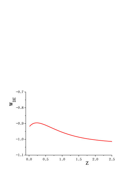
as well as on the effective dark-energy equation-of-state parameter
| (4.33) |
Additionally, we will use the redshift as the independent variable.
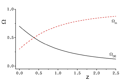
We evolve equations the Friedmann equation (4.8), (4.9) numerically and in Fig. 1 we depict the evolution of and . As we observe, we obtain the usual thermal history of the universe, with the sequence of matter and dark-energy epochs. Additionally, in Fig. 2 we present the corresponding effective dark-energy equation-of-state parameter . Interestingly enough we see that the effective dark energy crosses slightly into the phantom regime during the evolution, a feature that shows the capabilities of the scenario. Indeed according to the definitions of the effective dark-energy density and pressure given above, one can deduce that can be quintessence-like, phantom-like, or exhibit the phantom-divide crossing during evolution.
5 Conclusions
In the symmetric teleparallel formulation of gravity one uses non-metricity instead of curvature. Since the non-metricity scalar differs from the standard Levi-Civita Ricci scalar by a total divergence term, namely , general relativity and symmetric teleparallel general relativity are equivalent at the level of equations. However, modifications of the form and are not equivalent, since they do not differ by a total derivative.
In the present work we formulated gravity and cosmology, by incorporating the boundary term alongside in the Lagrangian. First we have extracted the general field equations, and then we have applied them in a cosmological framework, namely to flat Friedmann-Robertson-Walker (FRW) metric. Making three connection choices, we finally obtained the corresponding modified Friedmann equations. As we showed, we acquired an effective dark-energy sector of geometrical origin, which can lead to interesting cosmological phenomenology. Additionally, one may obtain an effective interaction between matter and dark energy.
Using a specific example, we showed that we can obtain the usual thermal history of the universe, with the sequence of matter and dark-energy epochs, as required. Furthermore, as we saw, the effective dark-energy equation-of-state parameter can be quintessence-like, phantom-like, or cross the phantom-divide, features that show the capabilities of the scenario.
In summary, we saw that gravity is a novel class of gravitational modification, and its cosmological application leads to interesting features. However, there are many investigations that one should do before considering gravity as a candidate for the description of Nature. One should proceed to a detailed confrontation with data from Supernovae type Ia (SNIa), Baryonic Acoustic Oscillations (BAO), Cosmic Microwave Background Radiation (CMB), Cosmic Chronometer (CC) etc observations, in order to extract constrains on the involved functions and parameters, and examine whether the model can alleviate the tension. Moreover, one could try to perform a dynamical-system analysis, in order to bypass the complexities of the scenario and extract the global features of the evolution. Additionally, one could proceed to the investigation of perturbations in order to examine the tension as well as the effect on gravitational waves, however it should be pointed out that the theoretical framework for the description of perturbations in a general non-Riemannian geometry requires to extend the standard cosmological perturbation theory in the lines of [91], which in the case of symmetric teleparallel gravities may lead to perturbation spectrum reduction [92]. These necessary studies lie beyond the scope of the present work, and are left for future projects.
Acknowledgements
The research was supported by the Ministry of Higher Education (MoHE), through the Fundamental Research Grant Scheme (FRGS/1/2021/STG06/UTAR/02/1). ENS acknowledges the contribution of the LISA CosWG, and of COST Actions CA18108 “Quantum Gravity Phenomenology in the multi-messenger approach” and CA21136 “Addressing observational tensions in cosmology with systematics and fundamental physics (CosmoVerse)”.
Appendix A Derivation of field equations
In this appendix we provide the derivation of the field equations (3.7)–(3.8). The coincident gauge shall be taken while deriving (3.7), so that partial derivatives and covariant derivatives can be used interchangeably. As usual, throughout the appendix all the divergence terms contributing to the boundary terms of the integrals will be neglected during the derivations.
In order to derive (3.7), we perform the variation on the action (3.6) with respect to the metric to obtain
| (A.1) |
The variation of is given in the the following identity [81]
| (A.2) |
while the second term on the right-hand side of (A), after neglecting the divergence term, reads
| (A.3) |
On the other hand
| (A.4) |
Since we have
| (A.5) |
Substituting this into (A.4), gives
| (A.6) |
Moreover, we derive
| (A.7) |
By using the fact that , and (2.11), we obtain
| (A.8) |
Finally, Eq. (3.7) can be obtained after substituting (A.3) and (A.8) into (A).
Now, we apply the method of Lagrange multipliers to derive the connection field equation (3.8). In particular, we write
| (A.9) |
which implements both the torsion-free and curvature-free constraints is added to the action (3.6). Variation with respect to the affine connection reads
| (A.10) |
where we use the fact that the Ricci scalar depends only on the metric components. We calculate each term separately as follows:
| (A.11) |
| (A.12) |
| (A.13) |
After substituting these equations into (A.10) one arrives at
| (A.14) |
where we denote . The Lagrange multiplier terms can be eliminated if the symmetric part of the equation in the indices and is considered, which reads
| (A.15) |
Finally if we apply the operator to this equation and then follow the calculations as in [93], the Lagrange multiplier terms will be removed and we result to
| (A.16) |
Finally, taking into account of the symmetry of , we extract the connection field equation (3.8).
Appendix B Proof of relation (3.19)
In this appendix we extract the useful relation (3.19). Indeed it can arise as an immediate consequence of the following identity
| (B.1) |
where is an arbitrary scalar field. Firstly, the left-hand-side of (B.1) can be expanded as
| (B.2) |
As shown in [52] one has
| (B.3) |
which implies that the first term on the right-hand-side vanishes. Additionally, we use a second identity given in [52], namely
| (B.4) |
while a direct calculation gives
| (B.5) |
and
| (B.6) |
Summing these equations, one arrives at (B.1). Hence, by virtue of (3.18) and (B.1), we finally obtain relation (3.19).
References
- [1] L. Perivolaropoulos and F. Skara, New Astron. Rev. 95, 101659 (2022) [arXiv:2105.05208 [astro-ph.CO]].
- [2] E. Abdalla, G. Franco Abellán, A. Aboubrahim, A. Agnello, O. Akarsu, Y. Akrami, G. Alestas, D. Aloni, L. Amendola and L. A. Anchordoqui, et al. JHEAp 34, 49-211 (2022) [arXiv:2203.06142 [astro-ph.CO]].
- [3] E. N. Saridakis et al. [CANTATA], Springer, 2021, [arXiv:2105.12582 [gr-qc]].
- [4] S. Capozziello and M. De Laurentis, Phys. Rept. 509, 167 (2011) [arXiv:1108.6266 [gr-qc]].
- [5] L. Heisenberg, Phys. Rept. 796, (2019).
- [6] A. A. Starobinsky, Phys. Lett. B 91, 99 (1980).
- [7] A. De Felice and S. Tsujikawa, Living Rev. Rel. 13, 3 (2010) [arXiv:1002.4928 [gr-qc]].
- [8] S. Nojiri and S. D. Odintsov, Phys. Lett. B 631, 1 (2005) [arXiv:hep-th/0508049].
- [9] C. Erices, E. Papantonopoulos and E. N. Saridakis, Phys. Rev. D 99, no.12, 123527 (2019) [arXiv:1903.11128 [gr-qc]].
- [10] D. Lovelock, J. Math. Phys. 12, 498 (1971).
- [11] G. R. Bengochea and R. Ferraro, Phys. Rev. D 79, 124019 (2009) [arXiv:0812.1205 [astro-ph]].
- [12] Y. F. Cai, S. Capozziello, M. De Laurentis and E. N. Saridakis, Rept. Prog. Phys. 79, no.10, 106901 (2016) [arXiv:1511.07586 [gr-qc]].
- [13] G. Kofinas and E. N. Saridakis, Phys. Rev. D 90, 084044 (2014) [arXiv:1404.2249 [gr-qc]].
- [14] G. Kofinas and E. N. Saridakis, Phys. Rev. D 90, 084045 (2014) [arXiv:1408.0107 [gr-qc]].
- [15] J.M. Nester, H-J Yo, Chin.J.Phys. 37, 113 (1999).
- [16] J. B. Jimenez, L. Heisenberg and T. Koivisto, Phys. Rev. D, 98, 044048 (2018).
- [17] J. B. Jimenez, L. Heisenberg and T.S. Koivisto, Universe, 5, 173 (2019).
- [18] D. Iosifidis, A. C. Petkou and C. G. Tsagas, Gen. Rel. Grav. 51, no.5, 66 (2019) [arXiv:1810.06602 [gr-qc]].
- [19] F. D’Ambrosio, L. Heisenberg and S. Kuhn, Class. Quantum Grav., 39, 025013 (2022).
- [20] J. Lu, Y. Guo and G. Chee, arXiv:2108.06865 (2021).
- [21] S. Capozziello, V. De Falco and C. Ferrara, arXiv:2208.03011 [gr-qc] (2022).
- [22] D. Iosifidis, Class. Quant. Grav. 38, no.1, 015015 (2021) [arXiv:2007.12537 [gr-qc]].
- [23] D. Iosifidis, Eur. Phys. J. C 80, no.11, 1042 (2020) [arXiv:2003.07384 [gr-qc]].
- [24] J. Lu, X. Zhao and G. Chee, Eur. Phys. J. C, 79, 530 (2019).
- [25] J. B. Jiménez, L. Heisenberg, T. Koivisto and S. Pekar, Phys. Rev. D., 101, 103507 (2020)
- [26] F. K. Anagnostopoulos, S. Basilakos, and E. N. Saridakis, Phys. Lett. B, 822, 136634 (2021).
- [27] D. Zhao, Eur. Phys. J. C, 82, 303 (2022).
- [28] R. Solanki, A. De, S. Mandal and P. K.Sahoo, Phys. Dark Univ., 36, 101053 (2022).
- [29] R. Solanki, A. De and P. K. Sahoo, Phys. Dark Univ., 36, 100996 (2022).
- [30] L. Atayde and N. Frusciante, Phys. Rev. D, 104, 064052 (2021).
- [31] A. De, S. Mandal, J. T. Beh, T. H. Loo and P.K. Sahoo, Eur. Phys. J. C, 82, 72 (2022).
- [32] B. J. Theng, T. H. Loo and A. De, Chinese J. of Phys., 77, 1551 (2022).
- [33] R. H. Lin and X. H. Zhai, Phys. Rev. D, 103, 124001 (2021).
- [34] S. Mandal, D. Wang and P. K. Sahoo, Phys. Rev. D, 102, 124029 (2020).
- [35] N. Frusciante, Phys. Rev. D, 103, 0444021 (2021).
- [36] B. J. Barros, T. Barreiro1, T. Koivisto and N. J. Nunes, Phys. Dark Univ., 30, 100616 (2020).
- [37] W. Khyllep, A. Paliathanasis and J. Dutta, Phys. Rev. D, 103, 103521 (2021).
- [38] M. Adak, M. Kalay, and O. Sert, Int. J. Mod. Phys. D 15, (2006) 619-634.
- [39] W. Khyllep, J. Dutta, E. N. Saridakis and K. Yesmakhanova, Phys. Rev. D 107, no.4, 044022 (2023) [arXiv:2207.02610 [gr-qc]].
- [40] A. Lymperis, JCAP 2022(11), 018 (2022).
- [41] N. Dimakis, A. Paliathanasis and T. Christodoulakis, Class. Quant. Grav. 38, no.22, 225003 (2021) [arXiv:2108.01970 [gr-qc]].
- [42] F. Bajardi, D. Vernieri, S. Capozziello, Eur. Phys. J. Plus, 135, 912 (2020).
- [43] F. K. Anagnostopoulos, V. Gakis, E. N. Saridakis and S. Basilakos, Eur. Phys. J. C 83, no.1, 58 (2023) [arXiv:2205.11445 [gr-qc]].
- [44] A. De and T. H. Loo, Phys. Rev. D, 106, 048501 (2022).
- [45] H. Shabani, A. De and T.H. Loo, Eur. Phys. J. C., 83, 535 (2023) [arxiv: 2304.02949 [gr-qc]].
- [46] A. De, D. Saha, G. Subramaniam and A.K. Sanyal, arxiv: 2209.12120 [gr-qc].
- [47] G. Subramaniam et al., Fortschr. der Phys. (2023) [arxiv: 2304.02300 [gr-qc]].
- [48] G. Subramaniam et al., Phys. Dark Univ. 41, 101243 (2023) [arxiv: 2304.05031 [gr-qc]].
- [49] N. Dimakis, M. Roumeliotis, A. Paliathanasis, P.S. Apostolopoulos, T. Christodoulakis, arXiv:2210.10295 [gr-qc].
- [50] N. Dimakis, A. Paliathanasis, M. Roumeliotis, and T. Christodoulakis, Phys. Rev. D, 106, 043509 (2022).
- [51] Fabio D’Ambrosio, Shaun D.B. Fell, Lavinia Heisenberg and Simon Kuhn, Phys. Rev. D, 105, 024042 (2022).
- [52] A. De and T. H. Loo, Class. Quantum Grav. 40, 115007 (2023).
- [53] J. Beltran Jimenez, L. Heisenber, JCAP 08, 039 (2018).
- [54] D. Iosifidis and K. Pallikaris, JCAP 05, 037 (2023) [arXiv:2301.11364 [gr-qc]].
- [55] H. Shabani, A. De, T. H. Loo and E. N. Saridakis, [arXiv:2306.13324 [gr-qc]].
- [56] J. Shi, Eur. Phys. J. C 83, no.10, 951 (2023) [arXiv:2307.08103 [gr-qc]].
- [57] G. W. Horndeski, Int. J. Theor. Phys. 10, 363-384 (1974).
- [58] A. De Felice and S. Tsujikawa, Phys. Rev. D 84, 124029 (2011) [arXiv:1008.4236 [hep-th]].
- [59] C. Q. Geng, C. C. Lee, E. N. Saridakis and Y. P. Wu, Phys. Lett. B 704, 384-387 (2011) [arXiv:1109.1092 [hep-th]].
- [60] S. Bahamonde et al, Phys. Rev. D 100, 064018 (2019).
- [61] S. Bahamonde, G. Trenkler, L. G. Trombetta and M. Yamaguchi, Phys. Rev. D 107, no.10, 104024 (2023) [arXiv:2212.08005 [gr-qc]].
- [62] L. Jarv et al, Phys. Rev. D 97, 124025 (2018).
- [63] M. Runkla and O. Vilson, Phys. Rev. D 98, 084034 (2018).
- [64] S. Bahamonde, C. G. Böhmer and M. Wright, Phys. Rev. D 92, no.10, 104042 (2015).
- [65] S. Bahamonde et al., Rep. Prog. Phys. 86 026901 (2023).
- [66] S. Capozziello, V. De Falco and C. Ferrara, [arXiv:2307.13280 [gr-qc]].
- [67] A. Paliathanasis, Phys. Rev. D 95, no.6, 064062 (2017) [arXiv:1701.04360 [gr-qc]].
- [68] A. Paliathanasis, JCAP 08, 027 (2017) [arXiv:1706.02662 [gr-qc]].
- [69] G. Farrugia, J. Levi Said, V. Gakis and E. N. Saridakis, Phys. Rev. D 97, no.12, 124064 (2018) [arXiv:1804.07365 [gr-qc]].
- [70] C. Escamilla-Rivera and J. Levi Said, tension,” Class. Quant. Grav. 37, no.16, 165002 (2020) [arXiv:1909.10328 [gr-qc]].
- [71] M. Caruana, G. Farrugia and J. Levi Said, Eur. Phys. J. C 80, no.7, 640 (2020) [arXiv:2007.09925 [gr-qc]].
- [72] A. Paliathanasis, Universe 7, no.5, 150 (2021) [arXiv:2104.00339 [gr-qc]].
- [73] A. R. P. Moreira, J. E. G. Silva, F. C. E. Lima and C. A. S. Almeida, Phys. Rev. D 103, no.6, 064046 (2021) [arXiv:2101.10054 [hep-th]].
- [74] A. Paliathanasis and G. Leon, Eur. Phys. J. Plus 136, no.10, 1092 (2021) [arXiv:2106.01137 [gr-qc]].
- [75] A. Paliathanasis and G. Leon, Math. Methods Appl. Sci. 46, no.4, 3905-3922 (2023) [arXiv:2201.12189 [gr-qc]].
- [76] F. W. Hehl, G. D. Kerlick, P. van der Heyde, Zeitschrift für Naturforschung A 31, 111 (1976)
- [77] T. Harko,T. S. Koivisto, F. S. N. Lobo, G. J. Olmo, and D. Rubiera-Garcia, Coupling matter in modified Q gravity, Phys. Rev. D 98, 084034 (2018).
- [78] C. G. Boehmer and E. Jensko, Phys. Rev. D 104, no.2, 024010 (2021) [arXiv:2103.15906 [gr-qc]].
- [79] C. G. Boehmer and E. Jensko, [arXiv:2301.11051 [gr-qc]].
- [80] J. Beltrán Jiménez and T. S. Koivisto, Int. J. Geom. Meth. Mod. Phys. 19, no.07, 2250108 (2022) [arXiv:2202.01701 [gr-qc]].
- [81] Y. Xu, G. Li, T. Harko and S. D. Liang, gravity, Eur. Phys. J. C, 79, 708 (2019).
- [82] M. Hohmann, Phys. Rev. D 104, no.12, 124077 (2021) [arXiv:2109.01525 [gr-qc]].
- [83] J. D. Barrow and T. Clifton, Phys. Rev. D 73, 103520 (2006) [gr-qc/0604063].
- [84] L. Amendola, G. Camargo Campos and R. Rosenfeld, Phys. Rev. D 75, 083506 (2007) [astro-ph/0610806].
- [85] X. m. Chen, Y. g. Gong and E. N. Saridakis, JCAP 0904, 001 (2009) [arXiv:0812.1117 [gr-qc]].
- [86] M. B. Gavela, D. Hernandez, L. Lopez Honorez, O. Mena and S. Rigolin, JCAP 0907, 034 (2009) [arXiv:0901.1611 [astro-ph.CO]].
- [87] X. m. Chen, Y. Gong, E. N. Saridakis and Y. Gong, Int. J. Theor. Phys. 53, 469 (2014) [arXiv:1111.6743 [astro-ph.CO]].
- [88] W. Yang and L. Xu, Phys. Rev. D 89, no.8, 083517 (2014) [arXiv:1401.1286 [astro-ph.CO]].
- [89] V. Faraoni, J. B. Dent and E. N. Saridakis, Phys. Rev. D 90, no. 6, 063510 (2014) [arXiv:1405.7288 [gr-qc]].
- [90] N. Aghanim et al. [Planck], Astron. Astrophys. 641, A6 (2020) [erratum: Astron. Astrophys. 652, C4 (2021)] [arXiv:1807.06209 [astro-ph.CO]].
- [91] K. Aoki, S. Bahamonde, J. Gigante Valcarcel and M. A. Gorji, [arXiv:2310.16007 [gr-qc]].
- [92] L. Heisenberg, M. Hohmann and S. Kuhn, [arXiv:2311.05495 [gr-qc]].
- [93] M. Hohmann, Universe 7, no.5, 114 (2021). [arXiv:2104.00536 [gr-qc]].