Time-space bi-fractional drift-diffusion equation for anomalous electrochemical transport

Abstract

The Debye-Falkenhagen differential equation is commonly used as a mean-field macroscopic model for describing electrochemical ionic drift and diffusion in dilute binary electrolytes when subjected to a suddenly applied potential smaller than the thermal voltage. However, the ionic transport in most electrochemical systems, such as electrochemical capacitors, permeation through membranes, biosensors and capacitive desalination, the electrolytic medium is interfaced with porous, disordered, and fractal materials which makes the modeling of electrodiffusive transport with the simple planar electrode theory limited. Here we study a possible generalization of the traditional drift-diffusion equation of Debye and Falkenhagen by incorporating both fractional time and space derivatives for the charge density. The nonlocal (global) fractional time derivative takes into account the past dynamics of the variable such as charge trapping effects and thus subdiffusive transport, while the fractional space derivative allows to simulate superdiffusive transport.

I Introduction

For the design and fabrication of most electrochemical devices and systems (e.g. batteries Galuppini et al. (2023), fuel cells Tanner et al. (1997), electrochemical supercapacitors Hasyim et al. (2017); Janssen and Bier (2018), capacitive deionization for water desalination Biesheuvel and Bazant (2010)) the use of spatially-heterogeneous electrodes with porous structures is omnipresent. The same is for protein channels or cell membranes which allow permeation of ions from one electrolytic solution to another Bolintineanu et al. (2009). The movement of charged species in free solutions interfaced with porous structures is known to be a multi-scale process that involves on the one hand ionic currents over millimetres in length in electroneutral reservoirs and in micrometer-sized macropores, to form, on the other hand, nanometer-sized electric double layers in the electrodes’ pores Kant and Singh (2017). The pores of can be of different sizes and shapes, and can be enlarged, partially obstructed or even completely blocked in the course of time. Therefore, there is a growing interest in developing advanced theories of porous electrodes in order to better understanding the electric double layer phenomena, ion transport and charge storage in complex electrochemical systems.

The classical mean-field modelling of electrodiffusive transport in electrochemistry is done via the well-studied mathematical framework of Poisson–Nernst–Planck (PNP) Mirzadeh and Gibou (2014). The PNP model has been also successfully applied to the description of ionic currents in protein channels of biological membranes Jasielec (2021). It is basically a set of coupled nonlinear equations with partial derivatives in time and space of integer-order that capture the dynamics of the electric potential and ionic densities. For the simple case of a blocking electrochemical system (without Faradaic processes and without fluid flow) with a dilute, symmetric binary electrolyte of constant material properties that is, the valences of ions $z^{+}=z^{-}=z$, diffusivities $D^{+}=D^{-}=D$ and constant dielectric permittivity, independent of time or space, the dimensionless PNP model in the single coordinate $x$ perpendicular to the electrode or membrane (homogeneous in planes perpendicular to the $x$-axis) is constituted of the Nernst–Planck equations for mass conservation Schmuck and Bazant (2015); Schmuck (2011):

$${\partial_{\tilde{t}}\tilde{c}^{\pm}}=\partial_{\tilde{x}}\left({\partial_{\tilde{x}}{\tilde{c}}^{\pm}}\pm{\tilde{c}}^{\pm}{\partial_{\tilde{x}}\tilde{\phi}}\right)$$ (1)

with the Poisson’s equation:

$$-\eta^{2}\partial^{2}_{\tilde{x}}\tilde{\phi}=\tilde{c}^{+}-\tilde{c}^{-}$$ (2)

Here the reduced variables are: $\tilde{x}={x}/{l}$ ($l$ is a reference length scale), $\tilde{t}={t}/t_{D}$ ($t_{D}=l^{2}/D$ is a reference time scale), $\tilde{c}^{\pm}=c^{\pm}/\bar{c}$ (concentrations of positively and negatively charged ions with $\bar{c}$ a reference concentration), $\tilde{\phi}=ze\phi/(k_{B}T)$ ($\phi$ is the electrostatic potential), $\tilde{E}=zelE/(k_{B}T)=-{\partial_{\tilde{x}}\tilde{\phi}}$ (reduced electric field), $\eta=\lambda_{D}/l$ with $\lambda_{D}=\sqrt{\epsilon_{f}k_{B}T/(\bar{c}z^{2}e^{2})}$. The constants $k_{B}$ and $e$ are the Boltzmann constant and the elemental charge, respectively, $\epsilon_{f}$ is the dielectric permittivity of the solvent and $T$ is the thermodynamic temperature (both assumed to be a constant). In principle, this problem given by Eqs. 1 and 2 retains well enough the essential features of electrodiffusion dynamics Schmuck and Bazant (2015).

If we further consider the Debye-Falkenhagen linearization (i.e. system subjected to a suddenly applied potential smaller than the thermal voltage, thus producing small variation of the bulk density of ions with respect to the one in thermodynamic equilibrium Freire et al. (2006)), the PNP model given by Eqs. 1 and 2 reduces to the single diffusion-drift equation for the reduced ionic charge density $\tilde{\rho}=\rho/(ze\bar{c})$ (the difference between cationic and anionic concentrations) Bazant et al. (2004):

$${\partial_{\tilde{t}}\tilde{\rho}}={\partial^{2}_{\tilde{x}}\tilde{\rho}}-({2\tilde{c}_{0}}/{\eta^{2}})\tilde{\rho}$$ (3)

where ${2\tilde{c}_{0}}=\tilde{c}^{+}+\tilde{c}^{-}$ is a constant. Eq. 3 can also be rewritten in the form:

$${\partial_{\tilde{\tau}}\tilde{\rho}}={\partial^{2}_{\tilde{z}}\tilde{\rho}}-\tilde{\rho}$$ (4)

where $\tilde{\tau}=\tilde{t}({2\tilde{c}_{0}}/{\eta^{2}})$ and $\tilde{z}=\tilde{x}\sqrt{({2\tilde{c}_{0}}/{\eta^{2}})}$. For ease of notation, we shall drop the tildes and replace $\tau$ by $t$ and $z$ by $x$, such as Eq. 4 is now rewritten as:

$${\partial_{{t}}{\rho}}={\partial^{2}_{{x}}{\rho}}-{\rho}$$ (5)

We note for comparison that the general reaction-diffusion equation has the form Xin (2000):

$${\partial_{{t}}{\rho}}={\partial^{2}_{{x}}{\rho}}+f(\rho)$$ (6)

where the functional $f(\rho)$ is a nonlinear term pertinent to the process under consideration (e.g. $f(\rho)=\rho(1-\rho)$ for Kolmogorov, Petrovsky, and Piskunov (KPP) nonlinearity, $f(\rho)=\rho^{m}(1-\rho)$ for the $m^{\text{th}}$-order Fisher nonlinearity, etc.). The linear approximation of the PNP model given by Eq. 5 has been studied by several groups including Janssen Janssen (2019), Janssen and Bier Janssen and Bier (2018), Bazant et al. Bazant et al. (2004), Singh and Kant Singh and Kant (2013, 2014); Birla Singh and Kant (2014), and many others. It is best used for describing electrodiffusive dynamics at planar electrodes. However, in practice, these types of devices and systems unavoidably exhibit in a way or another anomalies in their electrical response and frequency dispersion of their properties due to their structural disorder, spatial heterogeneity, and wide spectrum of relaxation times. This renders the problem of describing their complex behavior restricted when using the traditional drift-diffusion model.

In particular, Eq. 5 considers changes in the reduced density of charge through a control volume to be linear and memoryless, due to the fact that we only use a first-order Taylor series approximation in space and time Wheatcraft and Meerschaert (2008). Differential equations with integer-order differential operator are actually defined in an infinitesimally small neighborhood of the point under consideration, and therefore are a tool for describing only local media. For the case of non-local media, the size of the control volume must be large enough compared to the scale(s) of the heterogeneity in the medium, which makes integer-order derivatives inadequate for describing media with heterogeneity. Furthermore, spatial heterogeneities are not necessarily static in the course of operation of the device or system, and therefore memory effects shall be taken into consideration.

For a proper theoretical modeling of anomalous transport, one can adopt fractional calculus to include fractional time and/or spacial derivatives Tarasov (2022). This is mainly attributed to the fact that the dynamics of transport processes substantially differs from the picture of classical transport owing to memory effects or spatial nonlocality of purely non-Markovian nature. Fractional calculus permits to deal with such situations via integrals and derivatives of any arbitrary real or complex order, and therefore permits to unify and extend integer-order integrals and derivatives used in classical models Mainardi (2022); Henry et al. (2010); Mainardi et al. (2001). Saichev and Zaslavsky Saichev and Zaslavsky (1997), Mainardi et al. Mainardi et al. (2001), and Gorenflo et al. Gorenflo et al. (2000) studied the generalization of the diffusion equation with fractional derivatives with respect to time and space, in which the first-order time derivative of the propagating quantity was replaced with a Caputo derivative and the second-order space derivative was replaced with a Riesz-Feller derivative. Kosztołowicz and Metzler Kosztołowicz and Metzler (2020) described the transport of an antibiotic in a biofilm using a time-fractional subdiffusion-absorption equation based on the Riemann- Liouville time-fractional derivative. Saxena, Mathai and Haubold studied extensively in a series of papers Saxena et al. (2004a, 2014a); Haubold et al. (2011); Saxena et al. (2014b, 2015) unified forms of fractional kinetic equations and fractional reaction-diffusion equations in which the time derivative is replaced by either the Caputo, Riemann-Liouville or a generalized fractional derivative as defined by Hilfer Hilfer (2000), and the space derivative is replaced by the Riesz–Feller derivative. Additional nonlinear terms pertinent to reaction processes are also considered. Fractional reaction-diffusion equations are of specific interest in a large class of science and engineering problems for describing non-Gaussian, non-Markovian, and non-Fickian phenomena.

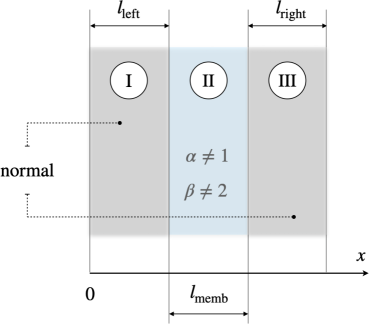
Figure 1: Nonhomogeneous membrane in which electrochemical transport is modeled with a bi-fractional Debye-Falkenhagen equation (Eq. (7), $\alpha\neq 1,\beta\neq 2$ with the conditions given in (8)). The $x$ axis is normal to the membrane plane.

The goal of this work is to study the bi-fractional (time and space) generalization of the (dimensionless) drift-diffusion equation of Debye and Falkenhagen (see section II, Eq. 7 below), and understand how do the fractional orders of differentiation affect the dynamics of the propagating quantity. In section III we provide the analytical solution to this equation in terms of Fox’s $H$-function, followed by numerical simulations in section IV for different sets of values for the fractional parameters.

II Model

We consider the the bi-fractional drift-diffusion equation in one dimension given by:

$${}^{\mathrm{c}}D_{t}^{\alpha}\rho=D_{x}^{\beta,\theta}\rho-\rho$$ (7)

subjected to the boundary and initial conditions

$$\rho(x=\pm\infty,t)=0,\qquad\rho(x,t=0)=\delta(x).$$ (8)

This model is a generalization of Eq. 5, and can describe for example the situation of anomalous ion diffusion through a membrane as shown in Fig. 1. In Eq. (7), the operator ${}^{\rm c}D^{\alpha}_{t}$ is the Caputo time fractional derivative of order $\alpha$ ($0<\alpha<1$) replacing the first order time derivative in Eq. 5, and $D^{\beta,\theta}_{x}$ is the Riesz-Feller space fractional derivative of order $\beta$ ($0<\beta<2$) replacing the second order space derivative Mainardi et al. (2001). The Caputo time-fractional derivative of order $\alpha$ ($m-1<\alpha<m,m\in\mathbb{N}$) of $f(t)$ is defined through the Laplace transform ($\tilde{f}(s)=\mathcal{L}[f(t);s]=\int_{0}^{\infty}e^{-st}f(t)dt,\;s\in\mathbb{C}$) by:

$$\mathcal{L}\left\{{}^{\rm c}D^{\alpha}_{t}f(t);s\right\}=s^{\alpha}\tilde{f}(s)-\sum_{r=0}^{m-1}s^{\alpha-r-1}f^{(r)}(0),$$ (9)

This lead to the integro-differential definition:

$$^{\rm c}D^{\alpha}_{t}f(t)\equiv\frac{1}{\Gamma(m-\alpha)}\int\limits_{0}^{t}\frac{f^{(m)}(\tau)d\tau}{(t-\tau)^{\alpha+1-m}},$$ (10)

that takes into account all past activities of the function up to the current time. For the case of $\alpha=m$, we have the traditional, memoryless integer-order derivative:

$${}^{\rm c}D^{\alpha}_{t}f(t)=\frac{d^{m}f(t)}{dt^{m}}$$ (11)

Whereas for a sufficiently well-behaved function $f(x)$, the Riesz-Feller space-fractional derivative of order $\beta$ ($0<\beta\leqslant 2$) and skewness $\theta$ ($|\theta|<\min\left\{\beta,2-\beta\right\}$) is defined in terms of its Fourier transform ($\hat{f}(k)=\mathcal{F}\{f(x);k\}=\int_{-\infty}^{\infty}e^{ikx}f(x)dx,\;k\in\mathbb{R}$) as Mainardi et al. (2001):

$$\mathcal{F}\left\{D^{\beta,\theta}_{x}f(x);k\right\}=-|k|^{\beta}e^{i(\mathrm{sgn}k)\theta\pi/2}\hat{f}(k)$$ (12)

In terms of integral representation, the Riesz-Feller derivative can be represented by: Saxena et al. (2014b):

$$D^{\beta,\theta}_{x}f(x) =\frac{\Gamma(1+\beta)}{\pi}\times$$

$$\left\{\sin\left[(\beta+\theta)\pi/2\right]\int\limits_{0}^{\infty}\frac{f(x+\xi)-f(x)}{\xi^{1+\beta}}d\xi\ \right.$$

$$\left.\sin\left[(\beta-\theta)\pi/2\right]\int\limits_{0}^{\infty}\frac{f(x-\xi)-f(x)}{\xi^{1+\beta}}d\xi\right\}$$ (13)

For the specific case of $\theta=0$, we have the symmetric operator with respect to $x$ that can be interpreted as:

$$D^{\beta,0}_{x}f(x)=-\left[-\frac{d^{2}}{dx^{2}}\right]^{\beta/2}$$ (14)

and Eq. 12 reduces to:

$$\mathcal{F}\left\{D^{\beta,0}_{x}f(x);k\right\}=-|k|^{\beta}\hat{f}(k)$$ (15)

III Analytical solutions

III.1 Case with $0<\alpha<1$, $\beta=2$

We start with the simple case of $\beta=2$ and skewness $\theta=0$, which makes Eq. (7) to reduce to the time fractional equation of the form

$$^{\rm c}D^{\alpha}_{t}\rho=\partial^{2}_{x}\rho-\rho.$$ (16)

Taking into account the Laplace transform of the Caputo fractional time derivative, Eq. (16) in the Laplace space takes the form:

$$s^{\alpha}\tilde{\rho}(x,s)-s^{\alpha-1}\rho(x,0)=\partial^{2}_{x}\tilde{\rho}(x,s)-\tilde{\rho}(x,s).$$ (17)

Using (8) and making the Fourier transform for both sides of Eq. (17), we come to

$$s^{\alpha}\hat{\tilde{\rho}}(k,s)-s^{\alpha-1}=-k^{2}\hat{\tilde{\rho}}(k,s)-\hat{\tilde{\rho}}(k,s).$$ (18)

Thus, the solution of Eq. (16) in the Laplace-Fourier space reads,

$$\hat{\tilde{\rho}}(k,s)=\frac{s^{\alpha-1}}{s^{\alpha}+1+k^{2}}.$$ (19)

III.1.1 Solution in the real-Laplace space

To get the solution in the real space, it is convenient to make the inverse Laplace and Fourier transforms with respect to $s$ and $k$, sequentially Mainardi et al. (2001). However, we might be interested in the solution obtained by the inverse Fourier transform with respect to $k$ and remained in the Laplace space with respect to time $t$. Formally, one can write this solution in the form

$$\tilde{\rho}(x,s)=\frac{1}{2\pi}\int\limits_{-\infty}^{\infty}\frac{s^{\alpha-1}}{s^{\alpha}+1+k^{2}}e^{-ixk}\,dk.$$ (20)

Introducing the notation $s^{\alpha}+1=a$ ($\mathrm{Re}(s)>0$ and $\mathrm{Re}(a)>0$), we have

$$\tilde{\rho}(x,s) = \frac{s^{\alpha-1}}{2\pi}\int\limits_{-\infty}^{\infty}\frac{e^{-ixk}\,dk}{a+k^{2}}$$ (21)

$$= \frac{s^{\alpha-1}}{2\pi}\int\limits_{-\infty}^{\infty}\frac{e^{-ixk}\,dk}{(k-\sqrt{a}i)(k+\sqrt{a}i)}.$$

The integrand in Eq. (21) is analytic everywhere except for the isolated singularities $k=\pm\sqrt{a}i$, where it has simple poles. For $x>0$, using the residue theorem, we have

$$\lim_{R\to\infty} \oint_{C_{R}}\frac{e^{-ikx}\,dk}{(k-\sqrt{a}i)(k+\sqrt{a}i)}$$ (22)

$$= -2\pi i\,\mathrm{res}_{k=-\sqrt{a}i}\left[\frac{e^{-ikx}}{(k-\sqrt{a}i)(k+\sqrt{a}i)}\right],$$

where the contour $C_{R}$ is shown in Fig.2a.

a) b)

Figure 2: The integration contours for (a) $x>0$ and (b) $x<0$, and poles of the integrand on the left-hand side for Eq. (21).

As $R\to\infty$, the integral over the arc of the circle tends to zero, because the integrand

$$\frac{e^{-ikx}}{(k+\sqrt{a}i)(k-\sqrt{a}i)}=\frac{e^{-ix\mathop{\mathrm{Re}}k}e^{x\mathop{\mathrm{Im}}k}}{(k+\sqrt{a}i)(k-\sqrt{a}i)},\quad\mathop{\mathrm{Im}}k<0$$

vanishes exponentially for $x>0$. Therefore,

$$\lim_{R\to\infty}\oint_{C_{R}}\frac{e^{-ikx}\,dk}{(k-\sqrt{a}i)(k+\sqrt{a}i)}=\int\limits_{-\infty}^{\infty}\frac{e^{-ikx}\,dk}{(k+\sqrt{a}i)(k-\sqrt{a}i)}.$$ (23)

Calculating the residue, we obtain

$$\mathrm{res}_{k=-\sqrt{a}i}\left[\frac{e^{-ikx}}{(k+\sqrt{a}i)(k-\sqrt{a}i)}\right]=-\frac{e^{-\sqrt{a}x}}{2\sqrt{a}i}.$$ (24)

Substituting the latter and (23) in Eq. (22), we obtain

$$\int\limits_{-\infty}^{\infty}\frac{e^{-ikx}\,dk}{(k+\sqrt{a}i)(k-\sqrt{a}i)}=\frac{\pi e^{-\sqrt{a}x}}{\sqrt{a}},\quad x>0.$$ (25)

Thus, Eq. (21) takes the form

$$\tilde{\rho}(x,s)=\frac{s^{\alpha-1}e^{-\sqrt{a}x}}{2\sqrt{a}},\quad x>0.$$ (26)

Similarly, for $x<0$ we consider the contour $C_{R}$ is shown in Fig.2b. The result for Eq. (21) in this case reads,

$$\tilde{\rho}(x,s)=\frac{s^{\alpha-1}e^{\sqrt{a}x}}{2\sqrt{a}},\quad x<0.$$ (27)

Thus, combining Eqs. (26) and (27) together, we come to

$$\tilde{\rho}(x,s)=\frac{s^{\alpha-1}e^{-\sqrt{a}|x|}}{2\sqrt{a}}.$$ (28)

Finally, using $a=s^{\alpha}+1$, we obtain

$$\tilde{\rho}(x,s)=\frac{s^{\alpha-1}}{2(s^{\alpha}+1)^{1/2}}\exp\left[-|x|(s^{\alpha}+1)^{1/2}\right].$$ (29)

We should note that for the time-fractional diffusion equation

$$^{\rm c}D^{\alpha}_{t}\rho=\partial^{2}_{x}\rho,$$ (30)

the solution in the Laplace-Fourier space reads,

$$\hat{\tilde{\rho}}(k,s)=\frac{s^{\alpha-1}}{s^{\alpha}+k^{2}}.$$ (31)

Thus, from Eq. (28) with $a=s^{\alpha}$, one can get the solution in agreement with Metzler and Klafter (2000),

$$\tilde{\rho}(x,s)=\frac{1}{2}s^{\alpha/2-1}\exp\left[-|x|s^{\alpha/2}\right].$$ (32)

III.1.2 Solution in the Fourier-time space

Unfortunately, the inverse Laplace transform of Eq. (29) is problematic. However, we can invert the Laplace transform from Eq. (19) following Langlands Langlands (2006). We rewrite Eq. (19) as

$$\hat{\tilde{\rho}}(k,s)=\frac{s^{\alpha-1}}{s^{\alpha}+1+k^{2}}=\frac{s^{\alpha-1}}{s^{\alpha}+k^{2}}\frac{1}{1+\frac{1}{s^{\alpha}+k^{2}}}.$$ (33)

Now by expanding the second fraction we have

$$\hat{\tilde{\rho}}(k,s)=\frac{s^{\alpha-1}}{s^{\alpha}+k^{2}}\sum_{r=0}^{\infty}\frac{(-1)^{r}}{(s^{\alpha}+k^{2})^{r}}=\sum_{r=0}^{\infty}\frac{(-1)^{r}s^{\alpha-1}}{(s^{\alpha}+k^{2})^{r+1}}.$$ (34)

From Podlubny (1999) we have the following Laplace transform

$$\mathcal{L}\left\{t^{\alpha r+\beta-1}E^{(r)}_{\alpha,\beta}(-at^{\alpha});s\right\}=\frac{r!s^{\alpha-\beta}}{(s^{\alpha}+a)^{r+1}},$$ (35)

where

$$E_{\alpha,\beta}(z)=\sum_{k=0}^{\infty}\frac{z^{k}}{\Gamma(\alpha k+\beta)}$$ (36)

is the Mittag-Leffler function. Thus, using Eq. (35) with $a=k^{2}$ and $\beta=1$, we can invert the Laplace transform in (34) to get

$$\hat{\rho}(k,t)=\sum_{r=0}^{\infty}\frac{(-1)^{r}t^{\alpha r}}{r!}E_{\alpha}^{(r)}(-k^{2}t^{\alpha}).$$ (37)

The derivatives of the Mittag-Leffler function can be expressed in terms of the $H$-function (see Appendix A)  Langlands (2006); Mathai et al. (2010),

$$E^{(r)}_{\alpha,\beta}(-z)=H^{1,1}_{1,2}\left[z\bigr{|}{\scriptsize\begin{matrix}(-r,1)\\ (0,1),(-\alpha r,\alpha)\end{matrix}}\right],$$ (38)

knowing that the generalized Mittag-Leffler function in terms of the Mellin-Barnes integral representation is given by Saxena et al. (2004a):

$$E_{\alpha,\beta}^{\gamma}(z)=\frac{1}{\Gamma(\gamma)}\frac{1}{2\pi i}\int_{\Omega}\frac{\Gamma(-\xi)\Gamma(\gamma+\xi)(-z)^{\xi}d\xi}{\Gamma(\alpha\xi+\beta)}$$ (39)

and thus:

$$E_{\alpha,\beta}^{\gamma}(z)=H^{1,1}_{1,2}\left[z\bigr{|}{\scriptsize\begin{matrix}(1-\gamma,1)\\ (0,1),(1-\beta,\alpha)\end{matrix}}\right].$$ (40)

The two-parameter Mittag-Leffler (Eq. 36) is obtained by setting $\gamma=1$ in Eq. 40. Now one can then rewrite Eq. (37) in the form

$$\hat{\rho}(k,t)=\sum_{r=0}^{\infty}\frac{(-1)^{r}t^{\alpha r}}{r!}H^{1,1}_{1,2}\left[k^{2}t^{\alpha}\bigr{|}{\scriptsize\begin{matrix}(-r,1)\\ (0,1),(-\alpha r,\alpha)\end{matrix}}\right].$$ (41)

III.1.3 Solution in the real-time space

Now we invert the Fourier transform in Eq. (41). To do this, we note that $\hat{\rho}(k,t)$ is an even function of $k$. For an even function $\hat{f}(k)=\hat{f}(-k)$, the Fourier transform reduces to the Fourier cosine transform,

$$f(x)=\frac{1}{2\pi}\int\limits_{-\infty}^{\infty}\hat{f}(k)e^{-ikx}\,dk=\frac{1}{\pi}\int\limits_{0}^{\infty}\hat{f}(k)\cos(kx)\,dk.$$ (42)

The inverse Fourier cosine transform can be calculated using the following relation for the cosine transform of the $H$-function Saxena et al. (2004b)

$$\int\limits_{0}^{\infty}k^{\rho-1}\cos(kx)H^{m,n}_{p,q}\left[ak^{\mu}\bigr{|}{\scriptsize\begin{matrix}(a_{p},A_{p})\\ (b_{q},B_{q})\end{matrix}}\right]\,dk$$

$$=\frac{\pi}{x^{\rho}}H^{n+1,m}_{q+1,p+2}\left[\frac{x^{\mu}}{a}\bigr{|}{\scriptsize\begin{matrix}(1-b_{q},B_{q}),(\frac{1}{2}+\frac{\rho}{2},\frac{\mu}{2})\\ (\rho,\mu),(1-a_{p},A_{p}),(\frac{1}{2}+\frac{\rho}{2},\frac{\mu}{2})\end{matrix}}\right].$$ (43)

Using the latter with $\rho=1$, $a=t^{\alpha}$, $\mu=2$, and $m,n,p,q$, $(a_{p},A_{p})$ and $(b_{q},B_{q})$ coefficients defined in Eq. (41), one can invert the Fourier transform in Eq. (41) to obtain

$$\rho(x,t) = \frac{1}{\pi}\sum_{r=0}^{\infty}\frac{(-1)^{r}t^{\alpha r}}{r!}\int\limits_{0}^{\infty}\cos(kx)H^{1,1}_{1,2}\left[k^{2}t^{\alpha}\bigr{|}{\scriptsize\begin{matrix}(-r,1)\\ (0,1),(-\alpha r,\alpha)\end{matrix}}\right]\,dk$$ (44)

$$= \frac{1}{|x|}\sum_{r=0}^{\infty}\frac{(-1)^{r}t^{\alpha r}}{r!}H^{2,1}_{3,3}\left[\frac{x^{2}}{t^{\alpha}}\bigr{|}{\scriptsize\begin{matrix}(1,1),(1+\alpha r,\alpha),(1,1)\\ (1,2),(1+r,1),(1,1)\end{matrix}}\right].$$

Next, using the following reduction formula Mathai et al. (2010)

$$H^{m,n}_{p,q}\left[z\bigr{|}{\scriptsize\begin{matrix}(a_{1},A_{1}),\ldots,(a_{p},A_{p})\\ (b_{1},B_{1}),\ldots,(b_{q-1},B_{q-1}),(a_{1},A_{1})\end{matrix}}\right]$$

$$=H^{m,n-1}_{p-1,q-1}\left[z\bigr{|}{\scriptsize\begin{matrix}(a_{2},A_{2}),\ldots,(a_{p},A_{p})\\ (b_{1},B_{1}),\ldots,(b_{q-1},B_{q-1})\end{matrix}}\right],$$ (45)

we can simplify Eq. (44) to

$$\rho(x,t)=\frac{1}{|x|}\sum_{r=0}^{\infty}\frac{(-1)^{r}t^{\alpha r}}{r!}H^{2,0}_{2,2}\left[\frac{x^{2}}{t^{\alpha}}\bigr{|}{\scriptsize\begin{matrix}(1+\alpha r,\alpha),(1,1)\\ (1,2),(1+r,1)\end{matrix}}\right].$$ (46)

Finally, using the property of the $H$-function Mathai et al. (2010),

$$z^{\sigma}H^{m,n}_{p,q}\left[z\bigr{|}{\scriptsize\begin{matrix}(a_{p},A_{p})\\ (b_{q},B_{q})\end{matrix}}\right]=H^{m,n}_{p,q}\left[z\bigr{|}{\scriptsize\begin{matrix}(a_{p}+\sigma A_{p},A_{p})\\ (b_{q}+\sigma B_{q},B_{q})\end{matrix}}\right],\;\sigma\in\mathbb{C},$$ (47)

with $\sigma=-1/2$, we come to

$$\rho(x,t)=\sum_{r=0}^{\infty}\frac{(-1)^{r}t^{\alpha(r-\frac{1}{2})}}{r!}H^{2,0}_{2,2}\left[\frac{x^{2}}{t^{\alpha}}\bigr{|}{\scriptsize\begin{matrix}(1+\alpha[r-\frac{1}{2}],\alpha),(\frac{1}{2},1)\\ (0,2),(r+\frac{1}{2},1)\end{matrix}}\right].$$ (48)

Together, Eqs. (19), (28), (41) and (48) provide the solution to the time fractional equation (16) in four different spaces with respect to the density arguments, namely $x\leftrightarrow k$, and $t\leftrightarrow s$.

III.2 Case with $0<\alpha<1$, $0<\beta<2$

The solution to the bi-fractional drift-diffusion Eq. (7) with $0<\alpha<1$, $0<\beta<2$, $\theta=0$ in real-time space can be obtained similarly to the time-fractional equation (16). The Laplace-Fourier transformations of Eq. (7) with the conditions given in (8) is:

$$\hat{\tilde{\rho}}(k,s)=\frac{s^{\alpha-1}}{s^{\alpha}+1+k^{\beta}}.$$ (49)

The result for $\rho(x,t)$ is found to be:

$$\rho(x,t)=\frac{1}{|x|}\sum_{r=0}^{\infty}\frac{(-1)^{r}t^{\alpha r}}{r!}H^{2,1}_{3,3}\left[\frac{|x|^{\beta}}{t^{\alpha}}\bigr{|}{\scriptsize\begin{matrix}(1,1),(1+\alpha r,\alpha),(1,\frac{\beta}{2})\\ (1,\beta),(r+1,1),(1,\frac{\beta}{2})\end{matrix}}\right].$$ (50)

Using Eq. (47) with $\sigma=-1/\beta$, one can rewrite (50) as

$$\rho(x,t) = \sum_{r=0}^{\infty}\frac{(-1)^{r}t^{\alpha(r-\frac{1}{\beta})}}{r!}$$ (51)

$$\times H^{2,1}_{3,3}\left[\frac{|x|^{\beta}}{t^{\alpha}}\bigr{|}{\scriptsize\begin{matrix}(1-\frac{1}{\beta},1),(1+\alpha[r-\frac{1}{\beta}],\alpha),(\frac{1}{2},\frac{\beta}{2})\\ (0,\beta),(r+1-\frac{1}{\beta},1),(\frac{1}{2},\frac{\beta}{2})\end{matrix}}\right].$$

IV Numerical results

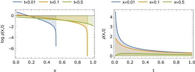
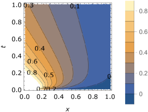
Figure 3: Plots of $\rho(x,t)$ given by Eq. 51 with $\alpha=1.0$, $\beta=2.0$ as a function of (a) $x$ for $t=0.01$, $0.1$, $0.5$, (b) $t$ for $x=0.01$, $0.1$, $0.5$ and (c) $x$ and $t$ (contour plot).

We calculate the obtained solutions for $\rho(x,t)$ governed by Eq. (7) with the boundary and initial conditions given by 8 for the four cases of (i) normal eletrodiffusion ($\alpha=1$, $\beta=2$), (ii) time-fractional eletrodiffusion ($0<\alpha<1$, $\beta=2$), (iii) space-fractional eletrodiffusion ($\alpha=1$, $0<\beta<2$) and (iv) bi-fractional electrodiffusion ($0<\alpha<1$, $0<\beta<2$) as given by Eq. 51. We fixed the upper limit of the summation to five terms, which is deemed sufficient to represent well enough the overall behavior of the variable $\rho(x,t)$. The Fox $H$-function can be calculated numerically using a simple rectangular approximation of the integrals Alhennawi et al. (2016). The function $\rho(x,t)$ is calculated for $x\in[-1,-\delta)\cup(\delta,1]$ and $t\in(\varepsilon,0.25]$, where $\delta>0$ and $\varepsilon>0$ are utilized to cut small locality around $x=0$, $t=0$, where the Fox $H$-function and $\rho(x,t)$ are not defined. We remind again that $\rho(x,t)$ described by Eq. (7) is a generalization of the integer-order Debye-Falkenhagen approximation (Eq. 5), whose validity is limited to the regime of small applied potentials.

First we consider the known integer-order case of $\alpha=1$, $\beta=2$ (i.e. Eq. 5). It is clear that at the limit $\alpha\to 1$ we obtain from Eq. 48 the following expression for $\rho(x,t)$:

$$\rho(x,t) = \frac{e^{-\sqrt{\frac{x^{2}}{t}}}}{2\sqrt{t}}$$ (52)

$$+ (-\sqrt{t}+\frac{t^{3/2}}{2}-\ldots)H^{1,0}_{1,1}\left[\frac{x^{2}}{t}\bigr{|}{\scriptsize\begin{matrix}(\frac{1}{2},1)\\ (0,2)\end{matrix}}\right]$$

The same can be found from Eq. 51 for $\alpha\to 1$, $\beta\to 2$. We recognize that the first term in Eq. 52 corresponds to the fundamental solution of the standard Fick’s diffusion equation $\partial_{t}\rho=\partial_{x}^{2}\rho$. Solutions to the integer-order case of Debye-Falkenhagen equation for different conditions has been previously provided mainly via numerical simulations and approximations (e.g. by using Padé approximation) Bazant et al. (2004); Feicht et al. (2016); Stout and Khair (2017), but here by using tools from fractional calculus we give an analytical expression as an infinite series of the Fox $H$-function. Plots of $\rho(x,t)$ for this case as a function of $x$ ($0.01<x<1$) for the different values of $t=0.01$, $0.1$, $0.5$ (in log-linear scale), and as a function of $t$ ($0.01<t<1$) for the different values of $x=0.01$, $0.1$, $0.5$ (in linear-linear scale) are shows in Figs. 3(a) and  3(b) respectively. Figs. 3(c) is the contour plot of $\rho(x,t)$ depicting its spatiotemporal dynamics. The solution depicting concentrations is always positive. It is an even function of $x$ and decays to zero for large values of $|x|$. It also decays to zero for large values of $t$.

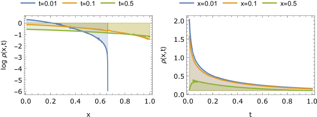
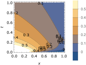
Figure 4: Plots of $\rho(x,t)$ given by Eq. 51 with for $\alpha=0.8$, $\beta=2.0$ as a function of (a) $x$ for $t=0.01$, $0.1$, $0.5$, (b) $t$ for $x=0.01$, $0.1$, $0.5$ and (c) $x$ and $t$ (contour plot).

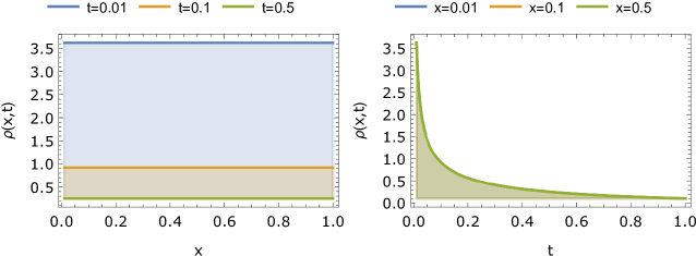
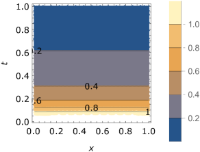
Figure 5: Plots of $\rho(x,t)$ given by Eq. 51 with for $\alpha=1.0$, $\beta=1.8$ as a function of (a) $x$ for $t=0.01$, $0.1$, $0.5$, (b) $t$ for $x=0.01$, $0.1$, $0.5$ and (c) $x$ and $t$ (contour plot).

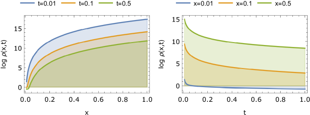
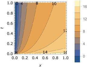
Figure 6: Plots of $\log(\rho(x,t))$ given by Eq. 51 with for $\alpha=0.8$, $\beta=1.8$ as a function of (a) $x$ for $t=0.01$, $0.1$, $0.5$, (b) $t$ for $x=0.01$, $0.1$, $0.5$ and (c) $x$ and $t$ (contour plot).

For the time-fractional anomalous case of $0<\alpha<1$, $\beta=2$, we verify that Eq. 51 reduces to Eq. 48. Similar to the previous case, plots of $\rho(x,t)$ as a function of $x$, as a function of $t$, and as a function of both $x$ and $t$ for $\alpha=0.8$, $\beta=2$ are shown in Fig. 4.

For the space-fractional anomalous case of $\alpha=1$, $0<\beta<2$, Eq. 51 simplifies to:

$$\rho(x,t)=(t^{-1/\beta} - t^{1-1/\beta}+\frac{1}{2}t^{2-1/\beta}-\ldots)$$ (53)

$$\times H_{2,2}^{1,1}\left[\frac{x^{\beta}}{t}\bigr{|}{\scriptsize\begin{matrix}(1-\frac{1}{\beta},1),(\frac{1}{2},\frac{\beta}{2})\\ (0,\beta),(\frac{1}{2},\frac{\beta}{2})\end{matrix}}\right]$$

which is plotted in Fig. 5 for the case of $\alpha=1$, $\beta=1.8$.

Finally, in Fig. 6 we show the variation of $\log\rho(x,t)$ vs. both variables $x$ and vs. $t$ for the general case of two fractional parameters, $\alpha=0.8$ and $\beta=1.8$. The propagating quantity $\rho(x,t)$ tends to accelerate as $x$ and $t$ increase, and thus the representation in log scale.

V Conclusion

The electrochemical modeling of electrified porous structures in contact with an electrolyte is quite challenging. The traditional mathematical tools are based on integer-order differential equations, which are more suited for homogeneous systems with planar geometries. When complex structures and coupled phenomena are involved, it is often required to further complement the existing models by additional approximations and assumptions which renders the problem even more difficult to solve. The theoretical and numerical results presented in this work show the possibilities that come with the use of both time and space bi-fractional-order derivatives for the case of the Debye-Falkenhagen equation, which is a simple and idealized model for electrodiffusion at low applied voltages. Eq. 51, with its extra two degrees of freedom, $\alpha$ and $\beta$, compared to the integer-order model (Eq. 52) is capable of deforming the spatiotemporal dynamics of the propagating quantity $\rho(x,t)$ in ways to account for subdiffusive and superdiffusive transports. While the physical interpretations of the fractional parameters remains unclear and need further studies, the mathematical solutions to this general problem can provide useful insights in anomalous electrodiffusion in heterogeneous media such as membranes, protein channels and electrochemical devices.

Appendix A Fox’s $H$-function

The Fox’s $H$-function Fox (1961) is defined by means of a Mellin-Barnes type integral in the following manner Mathai et al. (2009):

$$H^{m,n}_{p,q}(z) =H^{m,n}_{p,q}\left[z|^{(a_{p},A_{p})}_{(b_{q},B_{q})}\right]$$

$$=H^{m,n}_{p,q}\left[z|^{(a_{1},A_{1}),\ldots,(a_{p},A_{p})}_{(b_{1},B_{1}),\ldots,(b_{q},B_{q})}\right]$$

$$=\frac{1}{2\pi i}\int_{L}h(s)z^{-s}ds$$ (54)

with $h(s)$ given by the ratio of products of Gamma functions:

$$h(s)=\frac{\prod_{j=1}^{m}\Gamma(b_{j}+B_{j}s)\;\prod_{j=1}^{n}\Gamma(1-a_{j}-A_{j}s)}{\prod_{j={n+1}}^{p}\Gamma(a_{j}+A_{j}s)\;\prod_{j={m+1}}^{q}\Gamma(1-b_{j}-B_{j}s)}$$ (55)

$m,n,p,q$ are integers satisfying ($0\leqslant n\leqslant p$, $1\leqslant m\leqslant q$), $z\neq 0$, and $z^{-s}=\exp\left[-s(\ln|z|+i\arg z)\right]$, $A_{i},B_{j}\in\mathbb{R}_{+}$, $a_{i},b_{j}\in\mathbb{R}$ or $\mathbb{C}$ with $(i=1,2,\ldots,p)$, $(j=1,2,\ldots,q)$. The contour of integration $L$ is a suitable contour separating the poles $-(b_{j}+\nu)/B_{j}$, ($j=1,\ldots,m$; $\nu=0,1,2,\ldots$), of the gamma functions $\Gamma(b_{j}+B_{j}s)$ from the poles $(1-a_{\lambda}+k)/A_{\lambda}$, ($\lambda=1,\ldots,n$; $k=0,1,2,\ldots$) of the gamma functions $\Gamma(1-a_{\lambda}-A_{\lambda}s)$, that is $A_{\lambda}(b_{j}+\nu)\neq B_{j}(a_{\lambda-k-1})$. An empty product in 55, if it occurs, is taken to be one. The $H$-function contains a vast number of elementary and special functions as special cases. Detailed and comprehensive accounts of the matter are available in Mathai, Saxena, and Haubold Mathai et al. (2009), Mathai and Saxena Mathai et al. (1978), and Kilbas and Saigo Saigo et al. (2004)

References

- Galuppini et al. (2023) G. Galuppini, M. D. Berliner, D. A. Cogswell, D. Zhuang, M. Z. Bazant, and R. D. Braatz, Journal of Power Sources 573, 233009 (2023).
- Tanner et al. (1997) C. W. Tanner, K.-Z. Fung, and A. V. Virkar, Journal of the Electrochemical Society 144, 21 (1997).
- Hasyim et al. (2017) M. R. Hasyim, D. Ma, R. Rajagopalan, and C. Randall, Journal of The Electrochemical Society 164, A2899 (2017).
- Janssen and Bier (2018) M. Janssen and M. Bier, Physical Review E 97, 052616 (2018).
- Biesheuvel and Bazant (2010) P. Biesheuvel and M. Bazant, Physical review E 81, 031502 (2010).
- Bolintineanu et al. (2009) D. S. Bolintineanu, A. Sayyed-Ahmad, H. T. Davis, and Y. N. Kaznessis, PLoS computational biology 5, e1000277 (2009).
- Kant and Singh (2017) R. Kant and M. B. Singh, The Journal of Physical Chemistry C 121, 7164 (2017).
- Mirzadeh and Gibou (2014) M. Mirzadeh and F. Gibou, Journal of Computational Physics 274, 633 (2014).
- Jasielec (2021) J. J. Jasielec, Electrochem 2, 197 (2021).
- Schmuck and Bazant (2015) M. Schmuck and M. Z. Bazant, SIAM J. Appl. Math. 75, 1369 (2015).
- Schmuck (2011) M. Schmuck, Communications in Mathematical Sciences 9, 685 (2011).
- Freire et al. (2006) F. Freire, G. Barbero, and M. Scalerandi, Physical Review E 73, 051202 (2006).
- Bazant et al. (2004) M. Z. Bazant, K. Thornton, and A. Ajdari, Physical review E 70, 021506 (2004).
- Xin (2000) J. Xin, SIAM review 42, 161 (2000).
- Janssen (2019) M. Janssen, Physical Review E 100, 042602 (2019).
- Singh and Kant (2013) M. B. Singh and R. Kant, Journal of Electroanalytical Chemistry 704, 197 (2013).
- Singh and Kant (2014) M. B. Singh and R. Kant, The Journal of Physical Chemistry C 118, 8766 (2014).
- Birla Singh and Kant (2014) M. Birla Singh and R. Kant, The Journal of Physical Chemistry C 118, 5122 (2014).
- Wheatcraft and Meerschaert (2008) S. W. Wheatcraft and M. M. Meerschaert, Advances in Water Resources 31, 1377 (2008).
- Tarasov (2022) V. E. Tarasov, Mathematics 10, 1427 (2022).
- Mainardi (2022) F. Mainardi, Fractional calculus and waves in linear viscoelasticity: an introduction to mathematical models (World Scientific, 2022).
- Henry et al. (2010) B. I. Henry, T. A. Langlands, and P. Straka, in Complex Physical, Biophysical and Econophysical Systems (World Scientific, 2010) pp. 37–89.
- Mainardi et al. (2001) F. Mainardi, Y. Luchko, and G. Pagnini, Fractional Calculus and Applied Analysis 4, 153 (2001).
- Saichev and Zaslavsky (1997) A. I. Saichev and G. M. Zaslavsky, Chaos: an interdisciplinary journal of nonlinear science 7, 753 (1997).
- Gorenflo et al. (2000) R. Gorenflo, A. Iskenderov, and Y. Luchko, Fractional Calculus and Applied Analysis 3, 75 (2000).
- Kosztołowicz and Metzler (2020) T. Kosztołowicz and R. Metzler, Physical Review E 102, 032408 (2020).
- Saxena et al. (2004a) R. Saxena, A. Mathai, and H. Haubold, Astrophysics and Space Science 290, 299 (2004a).
- Saxena et al. (2014a) R. K. Saxena, A. M. Mathai, and H. J. Haubold, Axioms 3, 320 (2014a).
- Haubold et al. (2011) H. J. Haubold, A. M. Mathai, and R. K. Saxena, Journal of Computational and applied Mathematics 235, 1311 (2011).
- Saxena et al. (2014b) R. Saxena, A. Mathai, and H. Haubold, Journal of Mathematical Physics 55, 083519 (2014b).
- Saxena et al. (2015) R. K. Saxena, A. M. Mathai, and H. J. Haubold, Communications in Nonlinear Science and Numerical Simulation 27, 1 (2015).
- Hilfer (2000) R. Hilfer, in Applications of fractional calculus in physics (World Scientific, 2000) pp. 87–130.
- Metzler and Klafter (2000) R. Metzler and J. Klafter, Phys. Rep. 339, 1 (2000).
- Langlands (2006) T. A. M. Langlands, Phys. A 367, 136 (2006).
- Podlubny (1999) I. Podlubny, Fractional differential equations (Academic Press, New York, 1999).
- Mathai et al. (2010) A. M. Mathai, R. K. Saxena, and H. J. Haubold, The H-Function. Theory and applications. (Springer, Berlin, 2010).
- Saxena et al. (2004b) R. Saxena, A. Mathai, and H. Haubold, Astrophysics and Space Science 290, 299 (2004b).
- Alhennawi et al. (2016) H. R. Alhennawi, M. M. H. El Ayadi, M. H. Ismail, and H.-A. M. Mourad, IEEE Transactions on Vehicular Technology 65, 1957 (2016).
- Feicht et al. (2016) S. E. Feicht, A. E. Frankel, and A. S. Khair, Physical Review E 94, 012601 (2016).
- Stout and Khair (2017) R. F. Stout and A. S. Khair, Physical Review E 96, 022604 (2017).
- Fox (1961) C. Fox, Trans. Am. Math. Soc. 98, 395 (1961).
- Mathai et al. (2009) A. M. Mathai, R. K. Saxena, and H. J. Haubold, The -function: theory and applications (Springer Science & Business Media, 2009).
- Mathai et al. (1978) A. M. Mathai, R. K. Saxena, R. K. Saxena, et al., The -function with applications in statistics and other disciplines (John Wiley & Sons, 1978).
- Saigo et al. (2004) M. Saigo, A. A. Kilbas, et al., H-transforms: Theory and applications, Tech. Rep. (Chapman & Hall; CRC, 2004).