Imposing nonlocal boundary conditions in Galerkin-type methods based on non-interpolatory functions

Abstract

The imposition of inhomogeneous Dirichlet (essential) boundary conditions is a fundamental challenge in the application of Galerkin-type methods based on non-interpolatory functions, i.e., functions which do not possess the Kronecker delta property. Such functions typically are used in various meshfree methods, as well as methods based on the isogeometric paradigm. The present paper analyses a model problem consisting of the Poisson equation subject to non-standard boundary conditions. Namely, instead of classical boundary conditions, the model problem involves Dirichlet- and Neumann-type nonlocal boundary conditions. Variational formulations with strongly and weakly imposed inhomogeneous Dirichlet-type nonlocal conditions are derived and compared within an extensive numerical study in the isogeometric framework based on non-uniform rational B-splines (NURBS). The attention in the numerical study is paid mainly to the influence of the nonlocal boundary conditions on the properties of the considered discretisation methods.

1 Introduction

The problem of imposing inhomogeneous Dirichlet (essential) boundary conditions is well-known in the context of Galerkin-type meshfree methods. Such methods, as the element-free Galerkin (EFG) method [1], the reproducing kernel particle method (RKPM) [2] or the corrected smooth particle hydrodynamics (CSPH) method [3] use basis functions which do not satisfy the Kronecker delta property, i.e. a basis function associated with a particle does not necessarily vanish at other particles. Due to the non-interpolatory nature of the basis functions, the imposition of inhomogeneous Dirichlet boundary conditions in the meshfree approaches is not as straightforward as, for example, in the finite element method based on the classical interpolatory functions.

There exist many techniques for the imposition of classical essential boundary conditions in meshfree methods. For example, the applications of Lagrange multipliers [1], modified variational principles [1, 4], penalty methods [5, 6, 7], perturbed Lagrangian [8], modifying meshfree basis functions [9, 10, 11, 12, 13, 14], or coupling meshfree approaches and mesh-based techniques (namely, finite elements) [15, 16, 17, 18] can be mentioned. A novel method to treat Neumann and Dirichlet boundary conditions in meshfree methods for elliptic equations using nodal integration is presented in [19].

Non-interpolatory basis functions, such as non-uniform rational B-splines (NURBS), are also used in isogeometric analysis (IGA) [20, 21]. IGA is a computational technique which has been proposed with the aim to establish a direct connection between computer-aided design (CAD) and engineering analysis. Currently, the methods based on the isogeometric paradigm receive a lot of attention in the literature. A review of the mathematical foundation and recent results related to IGA can be found in [22, 23, 24]. Some trends and developments of IGA, as well as computer implementation aspects, are summarised in [25].

The imposition of inhomogeneous essential boundary conditions in the IGA framework is considered frequently (see e.g. [26, 27, 28, 29, 30]). A strong (direct) imposition is a possible way to treat such conditions, but weak imposition methods often are more efficient. For example, a weak imposition of essential boundary conditions is superior to strong imposition when solving various problems in fluid mechanics [31, 32]. In several situations considered in isogeometric analysis the imposition of boundary or coupling conditions is non-trivial, e.g., when the domain is composed of trimmed patches [33] or when the boundary of the physical domain is described as a curve or surface immersed in a regular grid [34, 35, 36].

Weak methods for the imposition of inhomogeneous essential boundary conditions in the context of meshfree methods usually are based on a certain modification of the basis functions (see e.g. [15, 9, 17]) or on a modification of the variational formulation of the problem. The well-known examples of methods from the latter class are the Lagrange multiplier method, the penalty method and Nitsche’s method. The Lagrange multiplier method is general and can be applied to the solution of various problems. However, it has some significant disadvantages, cf. [37, 38], among them is the difficulty of choosing a suitable Lagrange multiplier space. The penalty and Nitsche’s methods are attractive alternatives to the Lagrange multiplier method. A Nitsche formulation for spline-based finite elements has been applied to second- and fourth-order problems in [39].

The present paper deals with a model problem for Poisson equation with non-standard boundary conditions. Instead of the classical Dirichlet or Neumann boundary conditions, we consider a model problem involving nonlocal boundary conditions which can be used in order to express various nonlocal couplings between different parts of the model geometry. Such conditions, sometimes also called side conditions, appear in various mathematical models. For example, the models arising in thermoelasticity [40], thermodynamics [41], biological fluid dynamics [42], plasma physics [43], geology [44] or peridynamics [45] should be mentioned. Nonlocal multipoint constraints are used in the finite element analysis related to structural mechanics [46, 47]. A steady Poisson equation endowed with a generalised Robin boundary condition involving a Laplace–Beltrami operator on the boundary has been analysed in [48]. Overlapping Schwarz methods are based on a coupling the boundary of one subdomain with the interior of another subdomain, which is then solved iteratively. This approach has been applied in the isogeometric context in [49]. In [50], this coupled problem on overlapping subdomains (called overlapping multi-patch structure) is solved all at once. Hence, the coupling, which is performed point-wise at Greville abscissae, can be interpreted as an imposition of nonlocal constraints on parts of the boundary of each subdomain.

The main focus of this paper is the imposition of nonlocal boundary conditions for Galerkin methods using non-interpolatory basis functions. We investigate computationally the effects that such conditions have on the properties of the methods. While the numerical study is performed in the IGA framework, at least some of the insights can be applied in the context of other discretisation approaches too.

The paper is organised as follows. In Section 2, we formulate the model problem with nonlocal boundary conditions. Several variational formulations of the model problem are given in Section 3. We apply methods for the imposition of inhomogeneous Dirichlet-type nonlocal boundary conditions in the IGA context. Therefore, in Section 4 we shortly review the basic concepts and ideas used in IGA. The discretised equations are given in Section 5, and the results of the numerical study are presented in Section 6. Finally, we conclude the paper in Section 7 with a summary and several remarks.

2 Model problem

Partial differential equations (PDEs) with nonlocal boundary conditions receive a lot of attention in the literature from the point of view of both their theoretical investigation (see e.g. [51, 52]) and their numerical analysis (see [53, 54] and references therein).

In this paper we consider, as a model problem, the two-dimensional Poisson equation with mixed nonlocal boundary conditions: Find a function $u:\overline{\Omega}\rightarrow\mathbb{R}$, such that

$$\left\{\begin{array}[]{lll}-\nabla\cdot(\kappa\nabla u)=f&\text{in $\Omega$,}\rule{227.62204pt}{0.0pt}&\mbox{(a)}\\ u+\mathcal{L}_{1}[u]=g&\text{on $\Gamma_{D}$,}&\mbox{(b)}\\ \kappa\nabla u\cdot\mathbf{n}+\mathcal{L}_{2}[u]=h&\text{on $\Gamma_{N}$,}&\mbox{(c)}\end{array}\right.$$ (1)

where $\Omega\subset\mathbb{R}^{2}$ is an open and bounded domain with Lipschitz boundary $\partial\Omega\equiv\Gamma=\overline{\Gamma_{D}\cup\Gamma_{N}}$, $\Gamma_{D}\cap\Gamma_{N}=\emptyset$, $\Gamma_{D}\neq\emptyset$, $\mathbf{n}$ is the outward normal unit vector on $\partial\Omega$, $\kappa:\Omega\rightarrow\mathbb{R}$, $f:\Omega\rightarrow\mathbb{R}$, $g:\Gamma_{D}\rightarrow\mathbb{R}$ and $h:\Gamma_{N}\rightarrow\mathbb{R}$ are given functions, $\mathcal{L}_{1}:H^{1}(\Omega)\rightarrow\mathbb{R}$ and $\mathcal{L}_{2}:H^{1}(\Omega)\rightarrow\mathbb{R}$ are given linear functionals. We refer to (1b) and (1c) as Dirichlet- and Neumann-type nonlocal boundary conditions, respectively.

The linear functionals $\mathcal{L}_{1}$ and $\mathcal{L}_{2}$ define nonlocal parts of the boundary conditions. Various functionals can be used in order to express different types of nonlocal couplings. For example, the functional

$$\mathcal{L}[u]=\sum_{l}{\gamma_{l}u(\mathbf{x}_{l}^{*})}$$ (2)

for $\mathbf{x}_{l}^{*}\in\Omega$ represents discrete coupling, while the functional

$$\mathcal{L}[u]=\int_{\Omega}{\gamma u}\,\,\mathrm{d}\Omega$$ (3)

corresponds to more general integral coupling. The weights $\gamma_{l}$ and $\gamma$ are constants or functions measuring (controlling) the influence of the functionals.

Even though point evaluations are not well-defined in $H^{1}$, that means they are not suitable for the variational formulation we introduce in the following section, we can nonetheless mimic a point evaluation at $\mathbf{x}^{*}_{l}$ by introducing a suitable integral coupling. Let $\rho^{\delta}_{l}\in C^{\infty}(\Omega)$ be such that $\operatorname{supp}\rho^{\delta}_{l}\subseteq V_{\delta}(\mathbf{x}^{*}_{l})\cap\Omega$, where $V_{\delta}(\mathbf{x}^{*}_{l})$ is the $\delta$-neighbourhood of $\mathbf{x}^{*}_{l}$, and

$$\int_{\Omega}{\rho^{\delta}_{l}}\,\mathrm{d}\Omega=\gamma_{l}.$$

Then the integral coupling functional as in (3)

$$\mathcal{L}^{\delta}[u]=\sum_{l}\int_{\Omega}{\rho^{\delta}_{l}u}\,\mathrm{d}\Omega$$

is well-defined for $u\in H^{1}(\Omega)$ and approximates the discrete coupling functional in (2). If $u$ is sufficiently smooth, i.e. $u\in H^{1+\varepsilon}(\Omega)$, then $\lim_{\delta\rightarrow 0}\mathcal{L}^{\delta}[u]$ is also well-defined and is equal to the discrete coupling functional in (2) for all continuous $u$.

Note that the existence and uniqueness of the solution to a boundary value problem with nonlocal boundary conditions is non-trivial, as one can see considering the following simple problem: Find $u:[0,1]\rightarrow\mathbb{R}$, such that

$$u^{\prime\prime}=f\quad\text{in $\Omega=(0,1)$}\\$$

and

$$u+\mathcal{L}[u]=0\quad\text{on $\partial\Omega$,}\\$$

with

$$\mathcal{L}[u]=-\int_{0}^{1}u\,\mathrm{d}\Omega.$$

For any solution $u(x)$ and constant $\lambda$, the function $u(x)+\lambda$ also solves the problem. Hence, it has no unique solution. A similar situation is depicted for a specific choice of the functional $\mathcal{L}[u]$ in LABEL:fig:10 (see Section 6).

A full theoretical investigation of the model problem (1) and its variational formulation is beyond the scope of this paper. In fact, the existence and uniqueness of the solution might be difficult to prove for such problems formulated on general domains. Existence and uniqueness studies are presented, for example, in papers [51, 52]. In this paper, we assume that the model problem (1) has a unique, sufficiently smooth solution.

3 Variational formulations

In this section, we present several variational formulations of the model problem (1). In particular, the variational formulations based on a strong or a weak imposition of the inhomogeneous Dirichlet-type nonlocal boundary condition (1b) are given.

3.1 Strong imposition of Dirichlet-type nonlocal boundary conditions

Let us introduce the trial function space

$$\mathcal{S}=\{u\in H^{1}(\Omega):u+\mathcal{L}_{1}[u]=g\text{ on }\Gamma_{D}\}$$

and the test function space

$$\mathcal{V}=\{w\in H^{1}(\Omega):w=0\text{ on }\Gamma_{D}\}.$$

In this way, the Dirichlet-type nonlocal boundary condition (1b) is built into the space of trial functions, i.e. this condition is imposed strongly.

After multiplying (1a) by $w\in\mathcal{V}$ and integrating by parts, the identity

$$-\int_{\Omega}{\kappa\nabla w\cdot\nabla u}\,\mathrm{d}\Omega+\int_{\Gamma}{w(\kappa\nabla u\cdot\mathbf{n})}\,\mathrm{d}\Gamma+\int_{\Omega}{wf}\,\mathrm{d}\Omega=0$$ (4)

is obtained. Then, the Neumann-type nonlocal boundary condition (1c), as well as the constraint (homogeneous boundary condition) $w|_{\Gamma_{D}}=0$, is applied, and the variational formulation of problem (1) is given as follows: Find $u\in\mathcal{S}$ such that

$$a(w,u)=\ell(w)\quad\forall w\in\mathcal{V},$$ (5)

where

$$a(w,u)=\int_{\Omega}{\kappa\nabla w\cdot\nabla u}\,\mathrm{d}\Omega+\int_{\Gamma_{N}}{w\mathcal{L}_{2}[u]}\,\mathrm{d}\Gamma\\$$

and

$$\ell(w)=\int_{\Omega}{wf}\,\mathrm{d}\Omega+\int_{\Gamma_{N}}{wh}\,\mathrm{d}\Gamma.$$

The variational formulation (5) is consistent with the strong form (1), i.e. the exact solution $u$ of the problem (1) is also the solution of the variational problem (5).

3.2 Weak imposition of Dirichlet-type nonlocal boundary condition

For a weak imposition of the inhomogeneous Dirichlet-type nonlocal boundary condition (1b), methods based on modifications of the identity (4) can be used.

Let us assume now that the trial and test function space both are $H^{1}(\Omega)$, i.e. $\mathcal{S}=\mathcal{V}=H^{1}(\Omega)$. That is, the inhomogeneous Dirichlet-type nonlocal condition is no longer enforced in the trial function space nor the homogeneous classical Dirichlet condition is enforced in the test function space. Instead, the identity (4) is modified by augmenting it with two additional terms:

$$\begin{split}&-\int_{\Omega}{\kappa\nabla w\cdot\nabla u}\,\mathrm{d}\Omega+\int_{\Gamma}{w(\kappa\nabla u\cdot\mathbf{n})}\,\mathrm{d}\Gamma+\int_{\Omega}{wf}\,\mathrm{d}\Omega\\ &\quad+\alpha\int_{\Gamma_{D}}{(\kappa\nabla w\cdot\mathbf{n})(u+\mathcal{L}_{1}[u]-g)}\,\mathrm{d}\Gamma-\beta\int_{\Gamma_{D}}{w(u+\mathcal{L}_{1}[u]-g)}\,\mathrm{d}\Gamma=0,\end{split}$$

where $\beta$ is the penalty parameter (a positive constant), and the constant $\alpha=0$ or $1$. If $\alpha=0$, we have the so-called penalty method, while the method with $\alpha=1$ is referred to as Nitsche’s method. The variational formulation of the problem (1) now is stated as follows: Find $u\in H^{1}(\Omega)$ such that

$$a(w,u)=\ell(w)\quad\forall w\in H^{1}(\Omega),$$ (6)

where

$$\begin{split}a(w,u)&=\int_{\Omega}{\kappa\nabla w\cdot\nabla u}\,\mathrm{d}\Omega+\int_{\Gamma_{N}}{w\mathcal{L}_{2}[u]}\,\mathrm{d}\Gamma-\int_{\Gamma_{D}}{w(\kappa\nabla u\cdot\mathbf{n})}\,\mathrm{d}\Gamma\\ &\quad-\alpha\int_{\Gamma_{D}}{(\kappa\nabla w\cdot\mathbf{n})(u+\mathcal{L}_{1}[u])}\,\mathrm{d}\Gamma+\beta\int_{\Gamma_{D}}{w(u+\mathcal{L}_{1}[u])}\,\mathrm{d}\Gamma\end{split}$$

and

$$\ell(w)=\int_{\Omega}{wf}\,\mathrm{d}\Omega+\int_{\Gamma_{N}}{wh}\,\mathrm{d}\Gamma-\alpha\int_{\Gamma_{D}}{(\kappa\nabla w\cdot\mathbf{n})g}\,\mathrm{d}\Gamma+\beta\int_{\Gamma_{D}}{wg}\,\mathrm{d}\Gamma.$$

The variational formulation (6) is consistent with the strong formulation of the problem (1).

In case of classical boundary conditions ($\mathcal{L}_{1}\equiv 0$, $\mathcal{L}_{2}\equiv 0$), $\alpha=1$ ensures the symmetry of the bilinear form $a(w,u)$. In case of nonlocal conditions, the bilinear form $a(w,u)$, in general, is non-symmetric. Asymmetry is a typical property of nonlocal problems and their discretisations. However, as we will see from the results obtained by our numerical study, in comparison to the penalty method ($\alpha=0$), the terms with $\alpha=1$ (Nitsche’s method) can slightly increase the accuracy of the results.

4 Isogeometric analysis: a brief overview

The numerical experiments will be performed in the isogeometric framework. Therefore, a brief overview of the concepts and ideas used in isogeometric analysis is given in this section. First of all, B-splines and NURBS, which are the basic computer-aided geometric design (CAGD) tools applied in IGA, are introduced. Then, the isoparametric approach for the approximation of an unknown solution is shortly described. A comprehensive description of NURBS, their properties and related algorithms can be found, for example, in [55, 56]. For more details related to IGA, see [20].

4.1 B-splines and NURBS

First of all, let us define B-splines, which are progenitors of NURBS. A finite sequence of non-decreasing real values $\Xi=(\xi_{1},\xi_{2},\dotsc,\xi_{n+p+1})$, with $\xi_{i}<\xi_{i+p}$ for all $i\in\{2,\ldots,n\}$ and, without loss of generality, $\xi_{1}=0$ and $\xi_{n+p+1}=1$, is called a knot vector. Here $p$ is the polynomial order (degree) of the B-spline basis functions and $n$ is the number of basis functions. A knot vector in which the first and last knot values are repeated $p+1$ times is called an open knot vector. Such knot vectors satisfy simple interpolation properties for function value and derivatives up to order $p$ and therefore play an important role both in CAGD and IGA. For a given knot vector $\Xi$, the B-spline basis functions of degree zero are defined as

$$N_{i,0}(\xi)=\left\{\begin{aligned} &1&&\text{if $\xi_{i}\leqslant\xi<\xi_{i+1}$,}&\\ &0&&\text{otherwise.}&\end{aligned}\right.$$

For $p>0$, the B-spline basis functions $N_{i,p}(\xi)$ can be constructed by the Cox–de Boor recursive formula

$$N_{i,p}(\xi)=\frac{\xi-\xi_{i}}{\xi_{i+p}-\xi_{i}}N_{i,p-1}(\xi)+\frac{\xi_{i+p+1}-\xi}{\xi_{i+p+1}-\xi_{i+1}}N_{i+1,p-1}(\xi),$$

with the convention $\dfrac{0}{0}=0$.

Let $\Xi=(\xi_{1},\xi_{2},\dotsc,\xi_{n+p+1})$ and, in the two-dimensional case, $\mathcal{H}=(\eta_{1},\eta_{2},\dotsc,\eta_{m+q+1})$ be the knot vectors, where $p$ and $q$ are polynomial orders of B-splines, and $n$ and $m$ are numbers of basis functions. Then, the univariate and bivariate NURBS basis functions are defined as follows:

$$R_{i}^{p}(\xi)=\frac{\omega_{i}N_{i,p}(\xi)}{\sum_{\hat{i}=1}^{n}{\omega_{\hat{i}}N_{\hat{i},p}(\xi)}}\\$$

and

$$R_{i,j}^{p,q}(\xi,\eta)=\frac{\omega_{i,j}N_{i,p}(\xi)M_{j,q}(\eta)}{\sum_{\hat{i}=1}^{n}{\sum_{\hat{j}=1}^{m}{\omega_{\hat{i},\hat{j}}N_{\hat{i},p}(\xi)M_{\hat{j},q}(\eta)}}},$$

where $\omega_{i}$ and $\omega_{i,j}$ are weights (real positive numbers), $N_{i,p}$ and $M_{i,q}$ are the B-spline basis functions defined over the knot vectors $\Xi$ and $\mathcal{H}$, respectively. The NURBS curves and surfaces are constructed as linear combinations of NURBS basis functions:

$$\mathbf{C}(\xi)=\sum_{i=1}^{n}{\mathbf{B}_{i}R_{i}^{p}(\xi)}\\$$

and

$$\mathbf{S}(\xi,\eta)=\sum_{i=1}^{n}{\sum_{j=1}^{m}{\mathbf{B}_{i,j}R_{i,j}^{p,q}(\xi,\eta)}},$$

where $\mathbf{B}_{i}$ and $\mathbf{B}_{i,j}\in\mathbb{R}^{d}$ ($d=2,3$) are the control points. Since B-splines can be interpreted as NURBS where all weights are equal, we use the notation $N(\boldsymbol{\xi})$ to refer to both B-splines and NURBS.

In order to impose the Dirichlet-type nonlocal boundary condition (1b) strongly, we use Greville abscissae [57], which are well-known in the CAGD literature and which are widely used in isogeometric collocation methods [58, 59]. For a given knot vector $\Xi$, the Greville abscissae are $n$ points defined as

$$\overline{\xi}_{i}=\frac{1}{p}(\xi_{i+1}+\xi_{i+2}+\cdots+\xi_{i+p}).$$

The Greville abscissae naturally correspond to basis functions. The basis function $N_{i,p}$ attains its maximum close to the Greville abscissa $\overline{\xi}_{i}$, which is given by the average of the inner knots that define $N_{i,p}$. The Greville abscissae corresponding to the knot vector $\mathcal{H}$ are defined in the same way. Consequently, one can define Greville abscissae $(\overline{\xi}_{i},\overline{\eta}_{j})$ corresponding to tensor-product basis functions $N_{i,j}^{p,q}$. When using open knot vectors, the Greville abscissae on the boundary of the domain belong to those basis functions, that have non-vanishing support on the boundary.

4.2 Isogeometric approximation

Let us assume that the physical domain (model geometry) $\Omega\subset\mathbb{R}^{2}$ is represented by the geometrical mapping

$$\mathbf{x}:\widehat{\Omega}\rightarrow\Omega,$$

where $\widehat{\Omega}\subset\mathbb{R}^{2}$ is the parametric domain (in our setting we always assume $\widehat{\Omega}=(0,1)^{2}$). We also assume that this mapping is invertible, i.e. there exists the inverse mapping

$$\mathbf{x}^{-1}:\Omega\rightarrow\widehat{\Omega},$$

in short, we write $\boldsymbol{\xi}(\mathbf{x})$ for the inverse. In terms of the basis functions, the geometrical mapping is given as

$$\mathbf{x}(\boldsymbol{\xi})=\sum_{A\in\boldsymbol{\eta}^{s}}{\mathbf{x}_{A}N_{A}(\boldsymbol{\xi})},$$

where $\mathbf{x}_{A}$ are the control points and $\boldsymbol{\eta}^{s}$ is the index set.

Note that in isogeometric analysis the physical domain is often represented by a collection of subdomains, so-called patches. These patches are often trimmed, i.e., their parametric domain is not a full rectangle (or cuboid) but only a part of it, which is usually implicitly defined. We would like to point out, that the imposition of boundary conditions on trimmed domains is usually also performed weakly, see [60]. Similarly, coupling between patches may be performed weakly.

The approximation of the unknown solution $u$ in the parametric domain $\widehat{\Omega}$ is given by

$$\hat{u}^{h}(\boldsymbol{\xi})=\sum_{A\in\boldsymbol{\eta}^{s}}{u_{A}N_{A}(\boldsymbol{\xi})},$$

where $u_{A}$ are the control variables. In the physical domain $\Omega$, the approximation of $u$ is expressed by using the push-forward:

$$u^{h}(\mathbf{x})=\hat{u}^{h}\circ\mathbf{x}^{-1}=\sum_{A\in\boldsymbol{\eta}^{s}}{u_{A}N_{A}(\boldsymbol{\xi}(\mathbf{x}))}.$$

The control variables $\mathbf{u}=\{u_{A}\}$ are determined by solving the linear system

$$\mathbf{K}\mathbf{u}=\mathbf{f},$$

where $\mathbf{K}$ is the global left-hand side matrix, $\mathbf{f}$ is the global right-hand side vector. The matrix $\mathbf{K}$ and vector $\mathbf{f}$ can be assembled using either a Galerkin or a collocation method. The details of the configurations we consider are presented in the following section.

5 Discretisations of variational formulations

In this section, the variational formulations presented in Section 3 are discretised. The expressions of the global left-hand side matrices and the right-hand side vectors of the resulting discrete linear systems are given.

Let us assume that $\mathcal{S}^{h}$ and $\mathcal{V}^{h}$ are the discrete counterparts of the trial function space $\mathcal{S}$ and the test function space $\mathcal{V}$ defined in Section 3 ($\mathcal{S}^{h}\subset\mathcal{S}$, $\mathcal{V}^{h}\subset\mathcal{V}$). The approximate solutions of the considered variational problems (5) and (6) are represented as

$$u^{h}=v^{h}+g^{h},$$

where

$$v^{h}=\sum_{A\in\boldsymbol{\eta}^{s}\setminus\boldsymbol{\eta}_{g}^{s}}{u_{A}N_{A}(\mathbf{x})},$$

and $g^{h}=\Pi^{h}{g}$ is the interpolant or projector of the function $g$ onto the space of basis functions that are supported on the boundary $\Gamma_{D}$ and satisfy a nonlocal constraint (1b). The interpolant (projector) is expressed as

$$g^{h}=\sum_{A\in\boldsymbol{\eta}_{g}^{s}}{g_{A}N_{A}(\mathbf{x})},$$

where $\boldsymbol{\eta}_{g}^{s}$ is the set containing all indices of the basis functions supported on the boundary $\Gamma_{D}$, corresponding to Greville abscissae on the boundary.

In the IGA framework, the interpolant $\Pi^{h}{g}$ can be constructed by using the interpolation at the mapped Greville abscissae in the physical domain, the images of the Greville abscissae $\overline{\boldsymbol{\xi}}$ under the geometry mapping. The interpolation conditions

$$\Pi^{h}{g}(\mathbf{x}(\overline{\boldsymbol{\xi}}))=g(\mathbf{x}(\overline{\boldsymbol{\xi}}))$$

must be satisfied at the Greville abscissae $\overline{\boldsymbol{\xi}}$ associated with the Dirichlet boundary $\Gamma_{D}$.

Another approach to obtain $\Pi^{h}{g}$ is based on the computation of $L^{2}$-projection:

$$\int_{\Gamma_{D}}{w^{h}\bigl{(}\Pi^{h}{g}-g\bigr{)}}\,\mathrm{d}\Gamma=0\quad\forall w^{h}\in\mathcal{V}^{h}.$$

When the Dirichlet-type nonlocal boundary condition (1b) is imposed strongly, the control variables in the expressions of $v^{h}$ and $g^{h}$ are determined by the linear system

$$\underbrace{\left[\begin{array}[]{lr}\mathbf{K}^{(1)}&\mathbf{0}\\ \;\;\;\;{\mathbf{K}^{(2)}}\end{array}\right]}_{\eqcolon\mathbf{K}_{\mathrm{s}}}\left\{\begin{array}[]{c}\mathbf{u}_{f}\\ \mathbf{u}_{g}\end{array}\right\}=\left\{\begin{array}[]{c}\mathbf{f}\\ \mathbf{g}\end{array}\right\},$$

where

$$\mathbf{u}_{f}=\{u_{A}\},\quad A\in\boldsymbol{\eta}^{s}\setminus\boldsymbol{\eta}_{g}^{s},$$ (7)

$$\mathbf{u}_{g}=\{g_{A}\},\quad A\in\boldsymbol{\eta}_{g}^{s},$$

$$\mathbf{K}^{(1)}=[K_{AB}^{(1)}],\quad K_{AB}^{(1)}=\int_{\Omega}{\kappa\nabla N_{A}\cdot\nabla N_{B}}\,\mathrm{d}\Omega+\int_{\Gamma_{N}}{N_{A}\mathcal{L}_{2}[N_{B}]}\,\mathrm{d}\Gamma,\quad A,B\in\boldsymbol{\eta}^{s}\setminus\boldsymbol{\eta}_{g}^{s},$$

$$\mathbf{f}=\{f_{A}\},\quad f_{A}=\int_{\Omega}{N_{A}f}\,\mathrm{d}\Omega+\int_{\Gamma_{N}}{N_{A}h}\,\mathrm{d}\Gamma,\quad A\in\boldsymbol{\eta}^{s}\setminus\boldsymbol{\eta}_{g}^{s}.$$

However, the structure of the matrix $\mathbf{K}^{(2)}$ and the vector $\mathbf{g}$ depends on the method which is used for the imposition of the inhomogeneous Dirichlet-type nonlocal boundary condition. In case of the interpolation at the mapped Greville abscissae, $\mathbf{K}^{(2)}$ and $\mathbf{g}$ are expressed as

$$\mathbf{K}^{(2)}=[K_{AB}^{(2)}],\quad K_{AB}^{(2)}=N_{B}(\mathbf{x}(\overline{\boldsymbol{\xi}}_{A}))+\mathcal{L}_{1}[N_{B}](\mathbf{x}(\overline{\boldsymbol{\xi}}_{A})),\quad A\in\boldsymbol{\eta}_{g}^{s},\,B\in\boldsymbol{\eta}^{s},$$

$$\mathbf{g}=\{g_{A}\},\quad g_{A}=g(\mathbf{x}(\overline{\boldsymbol{\xi}}_{A})),\quad A\in\boldsymbol{\eta}_{g}^{s}.$$

If $L^{2}$-projection is applied, then

$$\mathbf{K}^{(2)}=[K_{AB}^{(2)}],\quad K_{AB}^{(2)}=\int_{\Gamma_{D}}{N_{A}(N_{B}+\mathcal{L}_{1}[N_{B}])}\,\mathrm{d}\Gamma,\quad A\in\boldsymbol{\eta}_{g}^{s},\,B\in\boldsymbol{\eta}^{s},$$

$$\mathbf{g}=\{g_{A}\},\quad g_{A}=\int_{\Gamma_{D}}{N_{A}g}\,\mathrm{d}\Gamma,\quad A\in\boldsymbol{\eta}_{g}^{s}.$$

The weak imposition of the inhomogeneous Dirichlet-type nonlocal boundary condition (1b) leads to the linear system

$$\underbrace{(\mathbf{K}^{(1)}-\mathbf{K}^{(3)}-\alpha\mathbf{K}^{(4)}+\beta\mathbf{K}^{(5)})}_{\eqcolon\mathbf{K}_{\mathrm{w}}}\mathbf{u}=\mathbf{f}-\alpha\mathbf{g}^{(1)}+\beta\mathbf{g}^{(2)},$$

where $\mathbf{K}^{(1)}$ and $\mathbf{f}$ are defined as in (7) with indices $A,B\in\boldsymbol{\eta}^{s}$, and

$$\mathbf{K}^{(3)}=[K_{AB}^{(3)}],\quad K_{AB}^{(3)}=\int_{\Gamma_{D}}{N_{A}(\kappa\nabla N_{B}\cdot\mathbf{n})}\,\mathrm{d}\Gamma,$$

$$\mathbf{K}^{(4)}=[K_{AB}^{(4)}],\quad K_{AB}^{(4)}=\int_{\Gamma_{D}}{(\kappa\nabla N_{A}\cdot\mathbf{n})(N_{B}+\mathcal{L}_{1}[N_{B}])}\,\mathrm{d}\Gamma,$$

$$\mathbf{K}^{(5)}=[K_{AB}^{(5)}],\quad K_{AB}^{(5)}=\int_{\Gamma_{D}}{N_{A}(N_{B}+\mathcal{L}_{1}[N_{B}])}\,\mathrm{d}\Gamma,$$

$$\mathbf{g}^{(1)}=\{g_{A}^{(1)}\},\quad g_{A}^{(1)}=\int_{\Gamma_{D}}{(\kappa\nabla N_{A}\cdot\mathbf{n})g}\,\mathrm{d}\Gamma,$$

$$\mathbf{g}^{(2)}=\{g_{A}^{(2)}\},\quad g_{A}^{(2)}=\int_{\Gamma_{D}}{N_{A}g}\,\mathrm{d}\Gamma,$$

$$A,B\in\boldsymbol{\eta}^{s}.$$

In contrast to the standard practice in the finite element analysis using models involving classical boundary conditions, the boundary control variables $\mathbf{u}_{g}$ are solved at the same time as the interior control variables $\mathbf{u}_{f}$.

Due to the nonlocal boundary conditions, the global left-hand side matrices $\mathbf{K}_{\mathrm{s}}$ and $\mathbf{K}_{\mathrm{w}}$, typically, are non-symmetric. Some examples of their sparsity patterns will be presented in the next section.

6 Numerical study

In this section we present the results of the numerical study which was conducted in order to examine and compare the methods for the imposition of inhomogeneous Dirichlet-type nonlocal boundary conditions.

6.1 Implementation details

The approximate solution methods for the model problem (1) have been implemented using GeoPDEs (version 3.1.0), a free IGA software suite [61, 62]. GeoPDEs can be launched both in MATLAB and GNU Octave environments.

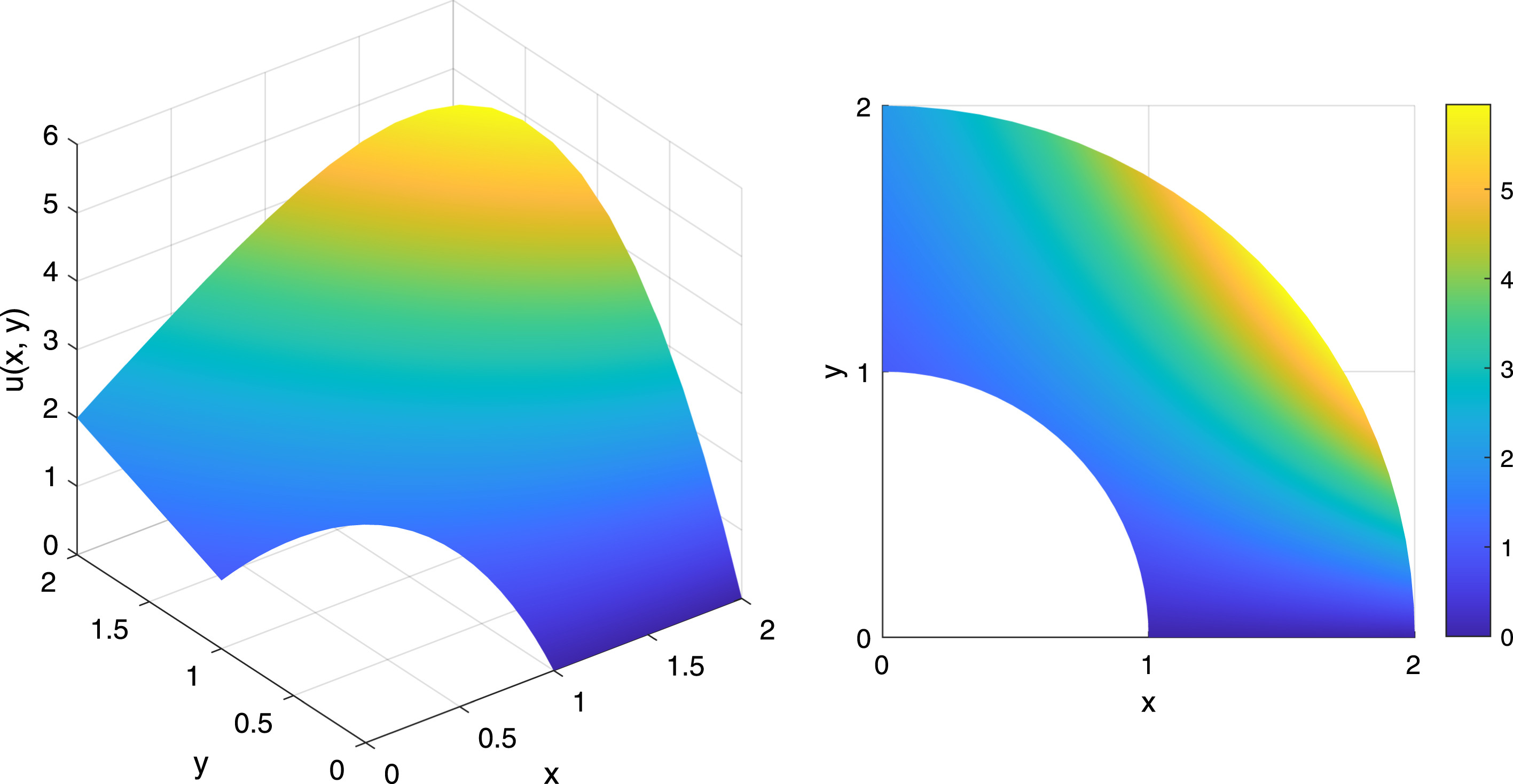
Fig. 1: The manufactured solution of the test problems. (For interpretation of the references to colour in this figure legend, the reader is referred to the web version of this article.)

The two-dimensional ($d=2$) problems with different (discrete or integral) nonlocal boundary conditions and the manufactured solution

$$u(x,y)=\exp{(x)}\cdot y,$$

see Figure 1, were analysed. The diffusivity coefficient in (1a) was assumed to be $\kappa(x,y)\equiv 1$. The problems were formulated on a quarter of a ring with the inner radius being equal to $1$ and the outer radius equal to $2$ (see Figure 2). The boundary part for the Neumann-type nonlocal boundary condition (1b) was assumed to be

$$\Gamma_{N}=\{(x,y):1\leqslant x\leqslant 2,y=0\}\cup\{(x,y):x=0,1\leqslant y\leqslant 2\},$$

while the Dirichlet-type nonlocal boundary condition (1b) was imposed on the rest of the boundary $\Gamma$ ($\Gamma_{D}=\Gamma\setminus\Gamma_{N}$). The domain parameterisation distributed together with GeoPDEs toolbox [62] in the file ring.mat was used.

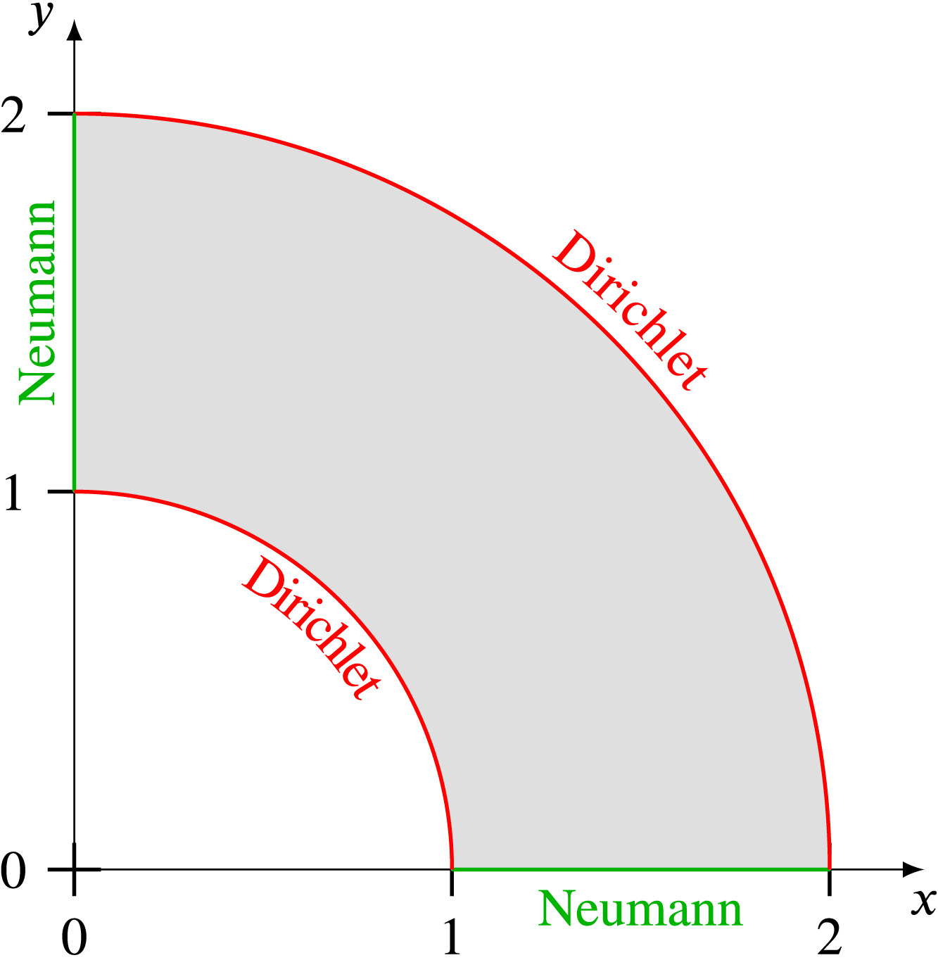
Fig. 2: The description of the test problems.

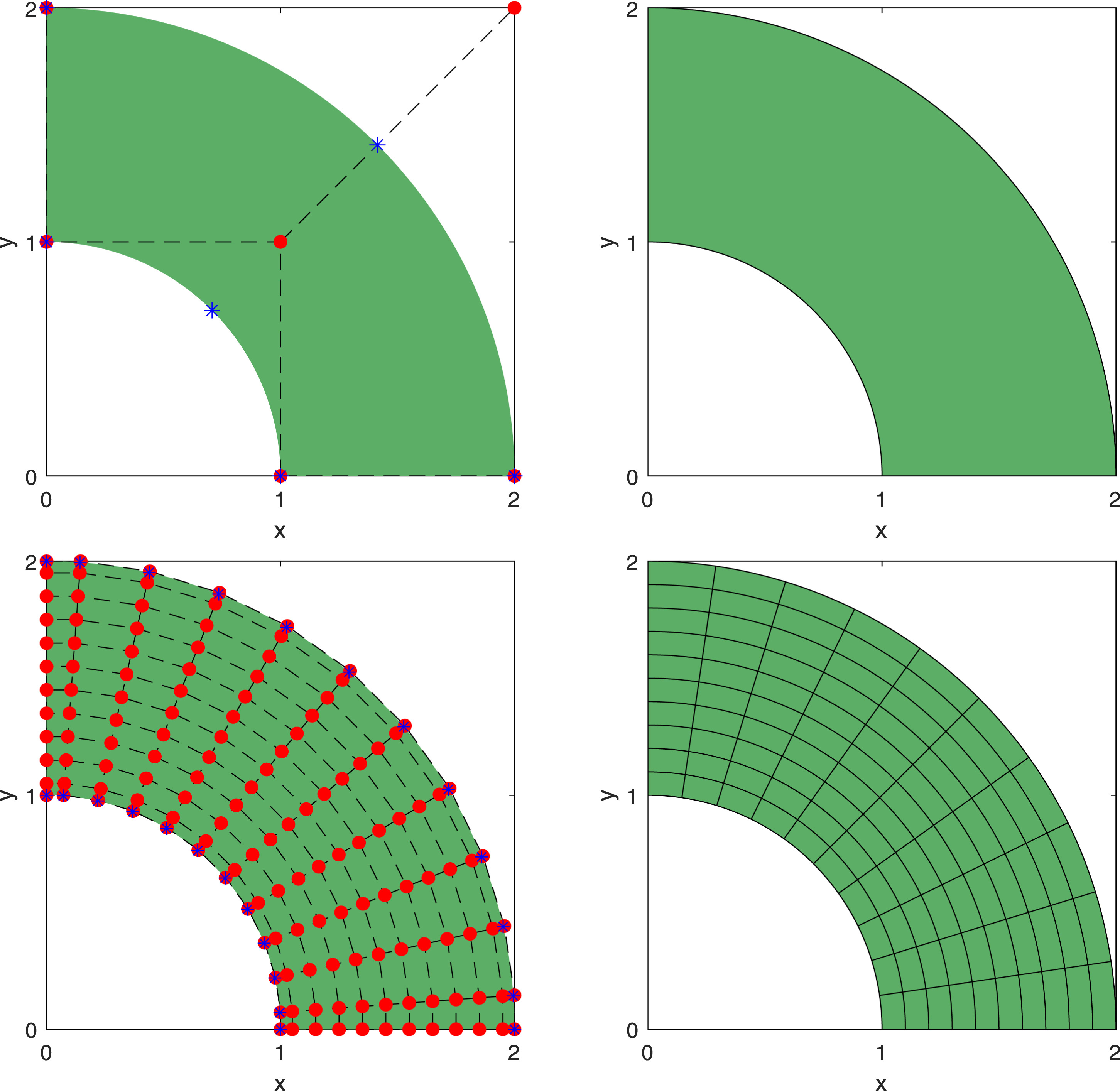
Fig. 3: The control meshes (left) and the physical meshes (right) before (top) and after (bottom) $k$-refinement. The control points are denoted as dots (red) and the images of the Greville abscissae associated with the boundary $\Gamma_{D}$ are denoted as stars (blue). (For interpretation of the references to colour in this figure legend, the reader is referred to the web version of this article.)

Two cases of nonlocal boundary conditions (1b) and (1c) were considered:

Case 1 (Discrete conditions).

$\mathcal{L}_{1}[u]=\mathcal{L}_{2}[u]=\gamma u(1,1)$

Case 2 (Integral conditions).

$\mathcal{L}_{1}[u]=\mathcal{L}_{2}[u]={\displaystyle\gamma\int_{\Omega}{u}\,\mathrm{d}\Omega}$

The role of the parameter (a real number) $\gamma$ is to control the influence of nonlocal terms. The case of $\gamma=0$ corresponds to the classical Dirichlet and Neumann boundary conditions (classical case). It is assumed that $\gamma=1$, if it is not mentioned otherwise.

In order to enforce a nonlocal discrete coupling which involves the value of the unknown function at the point $\mathbf{x}^{*}$ in the physical domain $\Omega$ (as defined by the functionals of Case 1), one needs to identify the corresponding point $\boldsymbol{\xi}^{*}$ in the parametric domain $\widehat{\Omega}$ by calculating the pull-back $\boldsymbol{\xi}^{*}=\mathbf{x}^{-1}(\mathbf{x}^{*})$, i.e. by solving the equation $\mathbf{x}({\boldsymbol{\xi}}^{*})=\mathbf{x}^{*}$. For this, the standard MATLAB/GNU Octave routine fsolve was used. Meanwhile, nonlocal integral couplings (as in Case 2) can be implemented using the integration techniques which are typically applied in the IGA framework.

The numerical results presented in this section were obtained using NURBS of polynomial orders $p=q=2$, $C^{1}$ continuity in both parametric directions and the physical mesh consisting of 10 $\times$ 10 knot spans. The control and physical meshes before and after $k$-refinement [20, 21] are shown in Figure 3. In all numerical experiments, the integration was performed using a standard, element-wise, $(p+1)\times(q+1)$ tensor-product Gauss quadrature rule. The penalty parameter $\beta=10^{2}$ was used unless it is stated otherwise. The resulting linear systems, as a rule, are dense therefore iterative solvers might not be efficient and direct solvers might be required. In the numerical study, the linear systems were solved using the left division operator ’\’, which is standard both in MATLAB and GNU Octave environments.

The accuracy of the results was estimated using the $L^{2}$-norm of the absolute error. The 2-norm condition number $\operatorname{cond}{(\bullet)}=\|\bullet\|_{2}\cdot\|\bullet^{-1}\|_{2}$ was used to estimate the conditioning of the global left-hand side matrices.

6.2 Results and discussion

In the numerical study we focused on the investigation of the previously described imposition methods for inhomogeneous Dirichlet-type nonlocal boundary conditions. In particular, we examine the influence of the penalty parameter $\beta$ as well as the influence of the nonlocal boundary conditions on the properties of the methods. The different methods were compared in terms of their accuracy and conditioning.

Influence of the penalty parameter

The weak methods for the imposition of inhomogeneous Dirichlet-type nonlocal boundary conditions (the penalty method and Nitsche’s method) depend on the penalty parameter $\beta$ which controls the coercivity of the corresponding bilinear form $a(w,u)$. Too large values of the penalty parameter $\beta$ yield a poorly conditioned global left-hand side matrix $\mathbf{K}_{\mathrm{w}}$. Therefore, it is necessary to find a suitable value of the penalty parameter $\beta$ which guarantees the coercivity of the bilinear form and leads to the desired accuracy of the numerical results.

We performed a parametric study to investigate the influence of the penalty parameter $\beta$ on the accuracy and conditioning of the methods applied to solve the problems with the classical and nonlocal boundary conditions.

Figure 4 depicts the $L^{2}$-norms of the absolute errors and the condition numbers of the global left-hand side matrices obtained using the penalty and Nitsche’s methods with various values of the penalty parameter $\beta$. The $L^{2}$-norms of the absolute error values and the condition numbers obtained using the methods independent on the penalty parameter are also referenced.

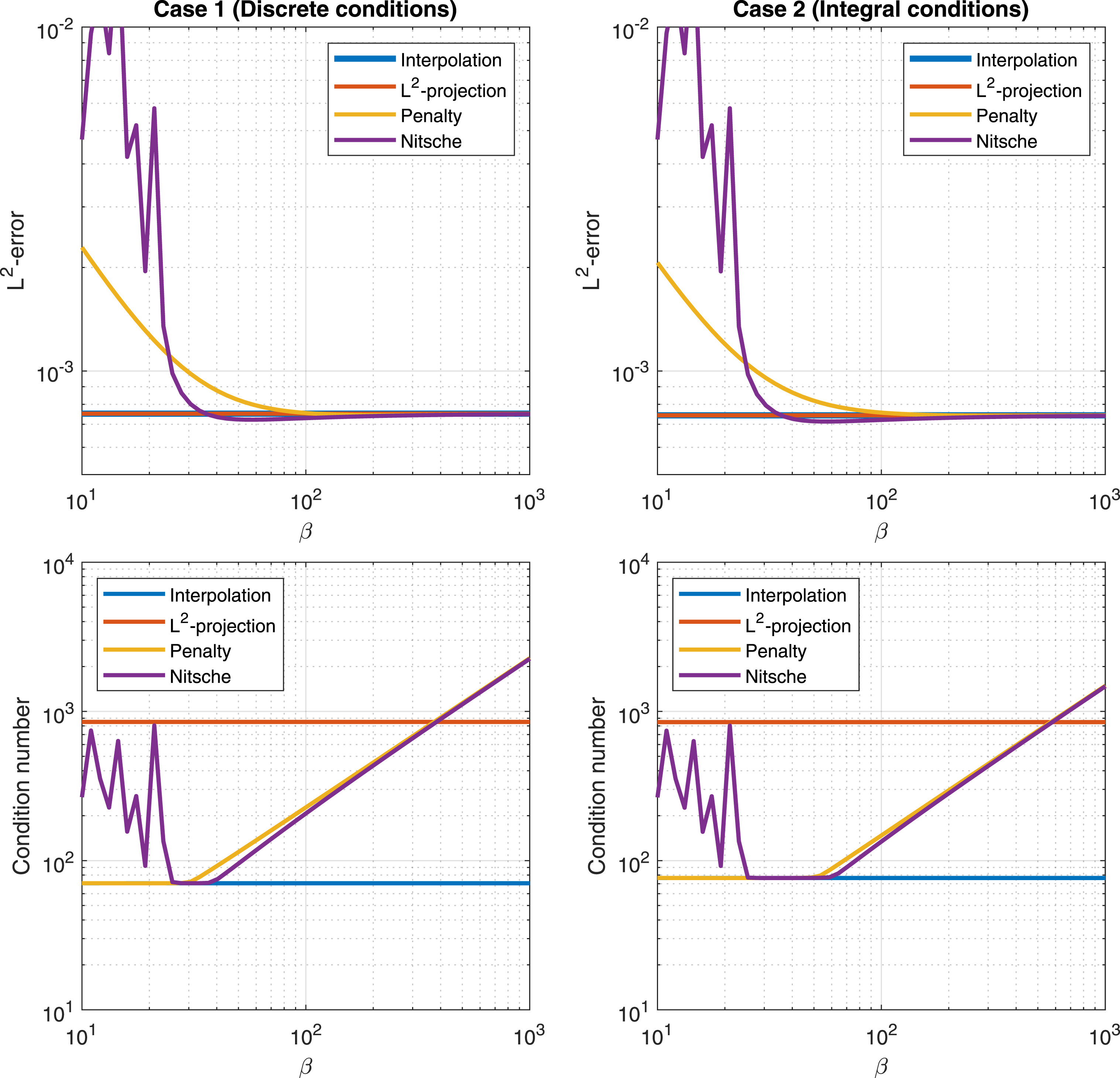
Fig. 4: The dependence of $L^{2}$-norm of the absolute error values (top) and the condition numbers of the global left-hand side matrices (bottom) on the values of the penalty parameter $\beta$. (For interpretation of the references to colour in this figure legend, the reader is referred to the web version of this article.)

As one can see from Figure 4 (top), the difference in the accuracy of the results obtained using two different methods with strongly imposed inhomogeneous Dirichlet-type nonlocal boundary condition (the interpolation at the Greville abscissae and the computation of $L^{2}$-projection) is insignificant. However, the application of the interpolation at the Greville abscissae leads to the methods with the global left-hand side matrices which has better conditioning (Figure 4, bottom). In fact, the method based on the interpolation at the Greville abscissae has the best conditioning among all four investigated approaches.

Comparing the weak imposition methods, the results obtained using Nitsche’s method are slightly more accurate than those obtained by using the penalty method, if the penalty parameter $\beta\sim 10^{2}$ (Figure 4, top). For smaller values of $\beta$ however, Nitsche’s method becomes more ill-conditioned and yields worse results. The difference becomes insignificant with larger values of the penalty parameter. Figure 4 (bottom) shows how the condition numbers of the resulting global left-hand side matrices grow when the value of the penalty parameter $\beta$ increases. It is also important to note, that Nitsche’s method (which is variationally consistent for the problem with classical boundary conditions) does not yield substantially better stability properties than the penalty method when nonlocal boundary conditions are enforced.

In Figure 5, we present the absolute errors of the numerical solutions obtained using various methods of the imposition of the inhomogeneous Dirichlet-type nonlocal boundary condition. Since the value of the penalty parameter $\beta$ used in the computations was quite large ($\beta=10^{2}$), the numerical results obtained using the weak imposition methods in terms of accuracy are comparable to those obtained when the discrete or integral Dirichlet-type nonlocal boundary conditions are imposed strongly. Note that in comparison to the penalty and Nitsche’s methods, the strong imposition methods result in lower errors at the boundary part for the Neumann-type boundary condition.

We investigated the convergence of the methods under knot refinement and degree elevation. The dependence of the $L^{2}$-error and of the condition number of the global left-hand side matrix on the number of control variables is presented in Figure 6. We see that optimal convergence is achieved in all cases, except the case of the weak imposition methods with $p=q=2$.

Note that the results in Figure 6 have been obtained using the fixed penalty parameter ($\beta=10^{2}$). However, the optimal convergence rate might be recovered if the penalty parameter value is properly adapted during refinement. As an example, penalty parameter values equalling the number of control variables ($\beta\sim 1/h^{2}$), following the suggestion from [37], were used in the experiment presented in Figure 7.

Influence of nonlocal boundary conditions

In comparison to the classical case, the appearance of nonlocal boundary conditions results in additional non-zero elements in the global left-hand side matrices. Examples of the sparsity patterns of these matrices are presented in Figure 8. Note that the structure of the global left-hand side matrices is implementation-dependent. In Figure 9, the sparsity patterns of the symmetric reverse Cuthill–McKee orderings are depicted.

LABEL:tab:1 presents the percentage of non-zero elements in the global left-hand side matrices and the bandwidths of their standard and symmetric reverse Cuthill–McKee orderings. One can see that, in comparison to the classical case, nonlocal boundary conditions increase the number of non-zero elements. The interpolation at the Greville abscissae leads to the most sparse matrices, while the matrices obtained using the penalty and Nitsche’s methods are the densest. Nonlocal integral boundary conditions increase the number of non-zero elements extremely and lead to full bandwidth matrices.

A parametric study was performed with the aim to investigate how nonlocal conditions affect the conditioning of the global left-hand side matrices $\mathbf{K}_{\mathrm{s}}$ and $\mathbf{K}_{\mathrm{w}}$. The test problems were solved using various values of the parameter $\gamma$.

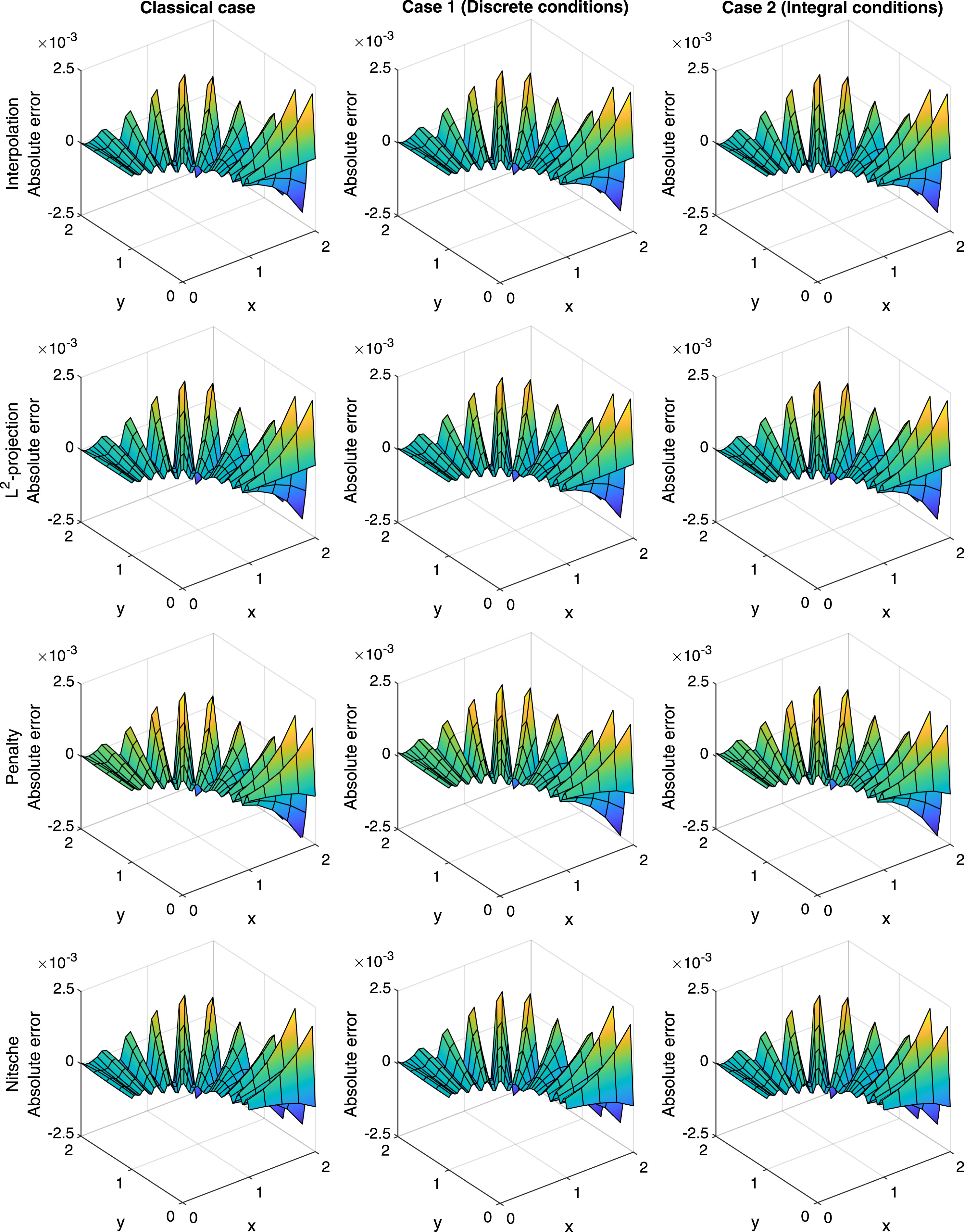
Fig. 5: The absolute errors of the numerical solutions obtained using different methods for the implementation of the inhomogeneous Dirichlet-type nonlocal boundary conditions.

LABEL:fig:10 clearly shows that nonlocal boundary conditions have a negative effect on the conditioning of the global left-hand side matrices. On the one hand, the condition numbers increase as the absolute value of the parameter $\gamma$ is increased. On the other hand, the problem becomes ill-conditioned around special values of $\gamma$, which are visible in the spikes in LABEL:fig:10. These values correspond to ill-posed problems or to problems which do not possess a unique solution as described in Section 2. The global left-hand side matrices corresponding to the methods with strongly imposed inhomogeneous Dirichlet-type nonlocal boundary conditions exhibit, in general, better conditioning in comparison to the matrices corresponding to the methods in which nonlocal boundary conditions are imposed weakly.

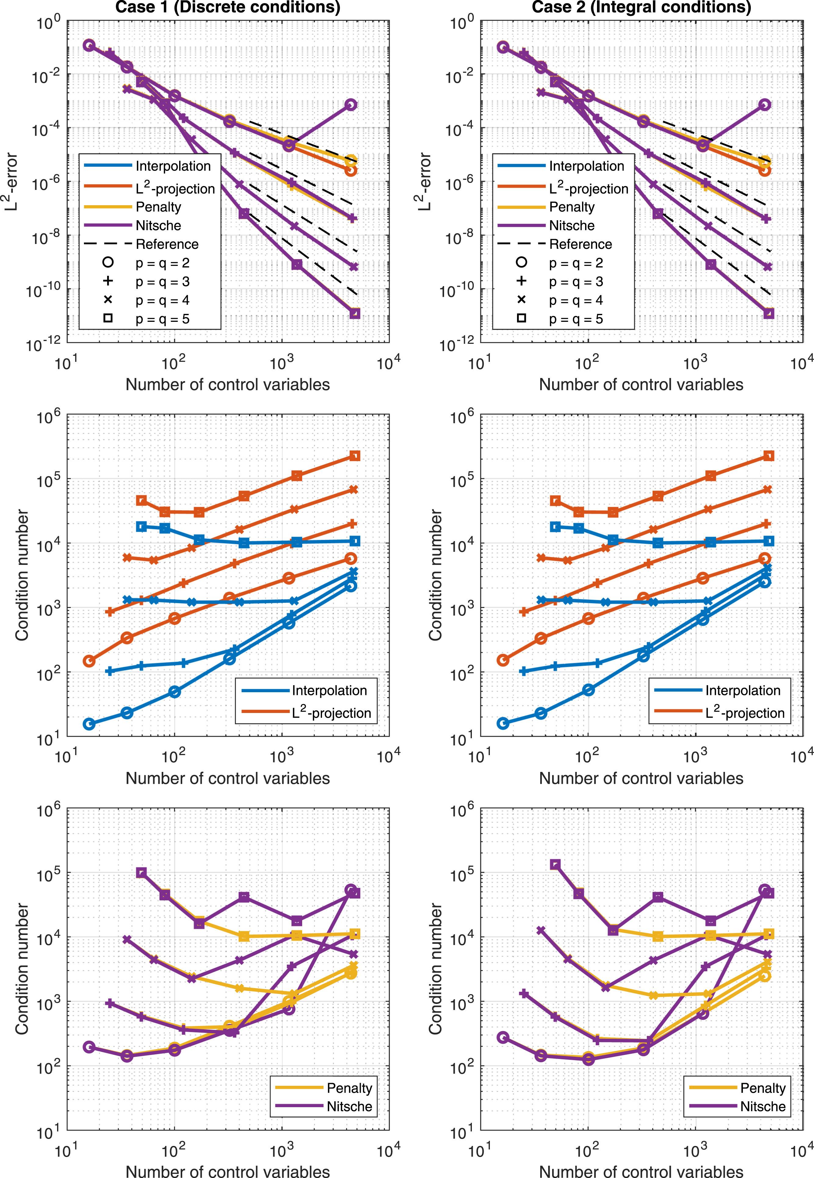
Fig. 6: The dependence of the $L^{2}$-error norms (top) and condition numbers of the global left-hand side matrices (middle and bottom) on the total number of control variables (degrees of freedom) under the refinement using basis functions of different degree. For the weak imposition methods we used a fixed penalty parameter $\beta$. Note that some lines are not visible. All methods except the penalty and Nitsche’s method in the case $p=q=2$ converge with the same rate. (For interpretation of the references to colour in this figure legend, the reader is referred to the web version of this article.)

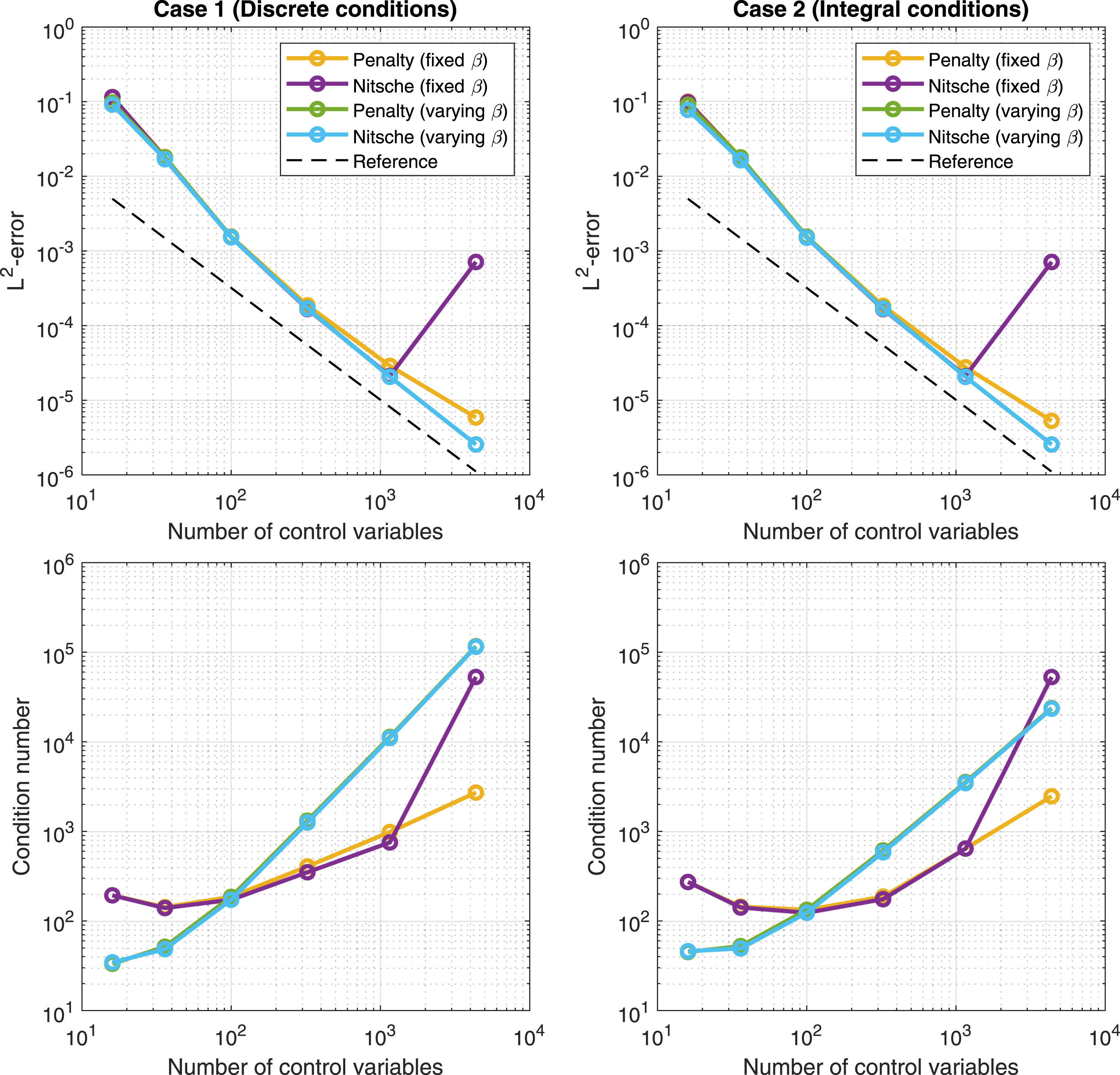
Fig. 7: The dependence of the $L^{2}$-error norms (top) and condition numbers of the global left-hand side matrices (bottom) on the total number of control variables (degrees of freedom). We compared a fixed and varying penalty parameter $\beta$. (For interpretation of the references to colour in this figure legend, the reader is referred to the web version of this article.)

7 Summary and concluding remarks

Imposing inhomogeneous Dirichlet (essential) boundary conditions is an important issue in computational approaches using non-interpolatory basis functions. Such functions are used in various meshfree methods, as well as in isogeometric analysis.

In this paper, we considered a model problem consisting of the Poisson equation equipped with nonlocal boundary conditions. Strong and weak methods for the imposition of Dirichlet-type nonlocal boundary condition were derived and compared experimentally in the isogeometric framework. The influence of nonlocal boundary conditions on the properties of the methods was investigated. Based on the results of numerical study, we derived the following conclusions:

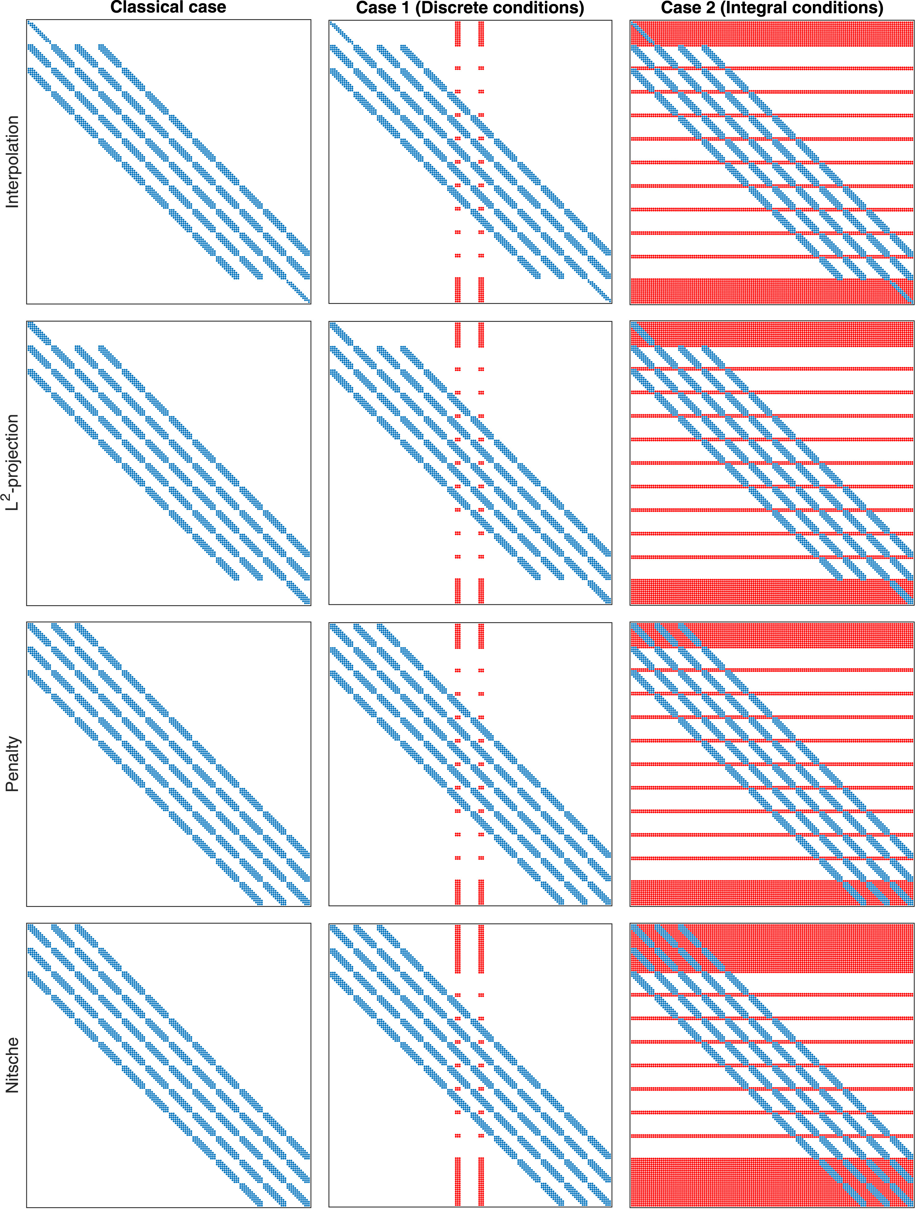
Fig. 8: The sparsity patterns of the global left-hand side matrices. The non-zero entries arisen due to nonlocal boundary conditions are marked in red. (For interpretation of the references to colour in this figure legend, the reader is referred to the web version of this article.)

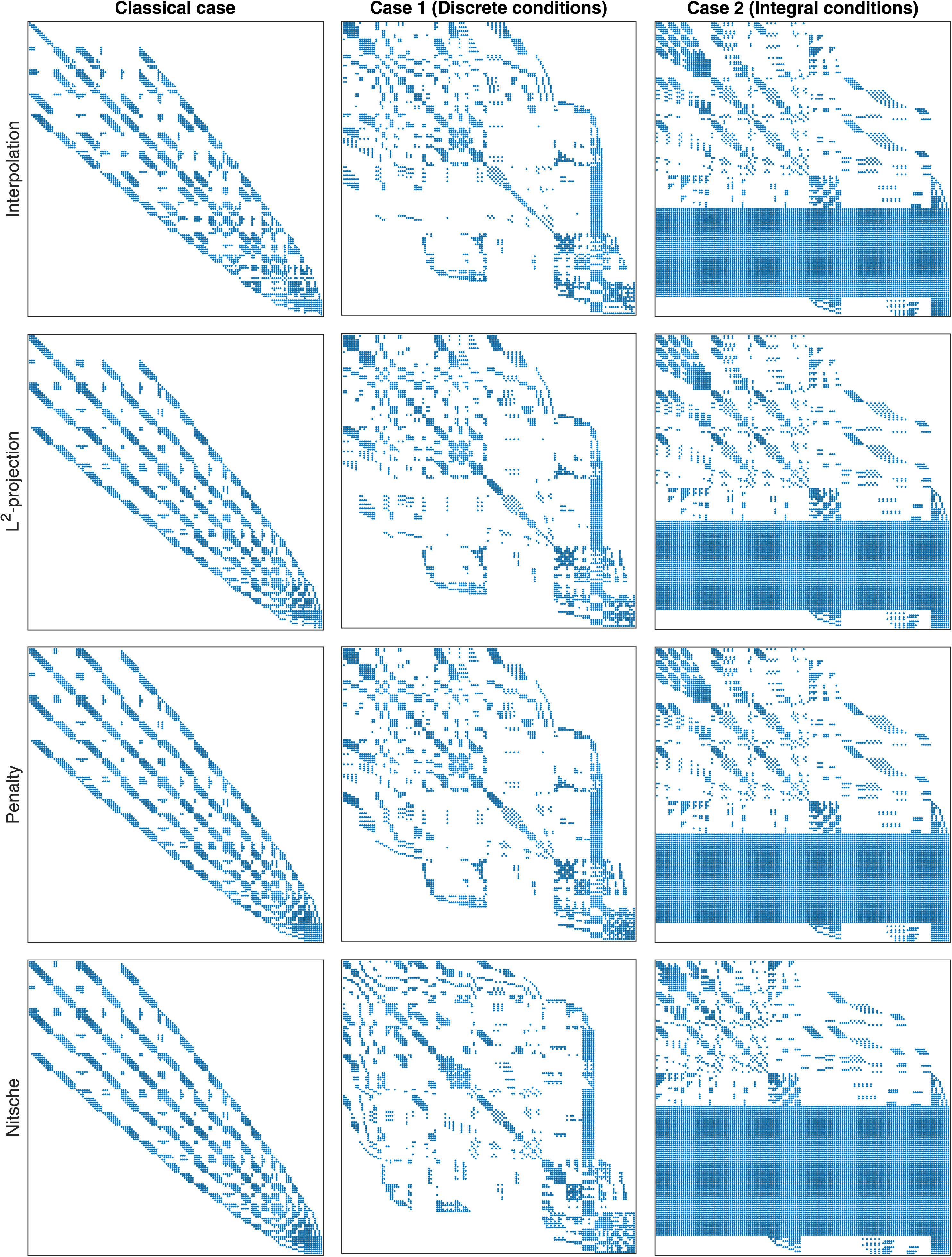
Fig. 9: The sparsity patterns of the symmetric reverse Cuthill–McKee orderings of the global left-hand side matrices.

1. Variational formulations with weakly imposed inhomogeneous Dirichlet-type nonlocal boundary conditions depend strongly on the choice of the penalty parameter. For small values of the penalty parameter, the accuracy is reduced. For larger values of the penalty parameter, the accuracy is improved, at the cost of the conditioning of the problem. The strong imposition method using the interpolation at the Greville abscissae has the best conditioning whereas the smallest error is reached using Nitsche’s method, if the penalty parameter is selected properly.

2. The appearance of nonlocal boundary conditions leads to an increased number of non-zero elements in the global left-hand side matrix. The weak imposition of Dirichlet-type nonlocal boundary condition leads to slightly denser global left-hand side matrices than those obtained when using the strong imposition methods. The global left-hand side matrices obtained when solving the problem with the nonlocal integral condition are much denser in comparison to the problems with nonlocal discrete boundary conditions.

3. Numerical evidence indicates that nonlocal boundary conditions might have a negative influence on the conditioning of the global left-hand side matrices.

Note that the density and structure of the resulting global left-hand side matrices also has an influence on the preferred choice of the solver, which may be of interest for future studies. The theoretical investigation of the considered variational formulations, as well as problems with nonlocal boundary conditions in general, is far from being a trivial task. Usually, the application of the Lax–Milgram theorem in the standard $H^{1}$ space is not possible. In some cases, the existence and uniqueness of the solution in the standard function spaces can be proved using embedding theorems. Otherwise, the introduction of special (weighted) function spaces is necessary. The reader is referred to [51, 52] for some examples of such investigations, while the theoretical investigation of the variational formulations considered in this paper is left as a future work.

CRediT authorship contribution statement

Svajūnas Sajavičius: Conceptualization, Methodology, Software, Investigation, Writing - original draft. Thomas Takacs: Validation, Formal analysis, Writing - review & editing.

References

- Belytschko et al. [1994] T. Belytschko, Y. Y. Lu, L. Gu, Element-free Galerkin methods, Int. J. Numer. Methods Engrg. 37 (1994) 229–256.
- Liu et al. [1995] W. K. Liu, S. Jun, Y. F. Zhang, Reproducing kernel particle methods, Internat. J. Numer. Methods Fluids 20 (1995) 1081–1106.
- Bonet and Lok [1999] J. Bonet, T.-S. L. Lok, Variational and momentum preservation aspects of smooth particle hydrodynamic formulations, Comput. Methods Appl. Mech. Engrg. 180 (1999) 97–115.
- Dumont et al. [2006] S. Dumont, O. Goubet, T. Ha-Duong, P. Villon, Meshfree methods and boundary conditions, Int. J. Numer. Methods Engrg. 67 (2006) 989–1011.
- Zhu and Atluri [1998] T. Zhu, S. N. Atluri, A modified collocation method and a penalty formulation for enforcing the essential boundary conditions in the element free Galerkin method, Comput. Mech. 21 (1998) 211–222.
- Bonet and Kulasegaram [2000] J. Bonet, S. Kulasegaram, Correction and stabilization of smooth particle hydrodynamics methods with applications in metal forming simulations, Int. J. Numer. Methods Engrg. 47 (2000) 1189–1214.
- Cho et al. [2008] J. Y. Cho, Y. M. Song, Y. H. Choi, Boundary locking induced by penalty enforcement of essential boundary conditions in mesh-free methods, Comput. Methods Appl. Mech. Engrg. 197 (2008) 1167–1183.
- Chu and Moran [1995] Y. A. Chu, B. Moran, A computational model for nucleation of solid–solid phase transformations, Model. Simul. Mater. Sci. Engrg. 3 (1995) 455–471.
- Gosz and Liu [1996] J. Gosz, W. K. Liu, Admissible approximations for essential boundary conditions in the reproducing kernel particle method, Comput. Mech. 19 (1996) 120–135.
- Günther and Liu [1998] F. C. Günther, W. K. Liu, Implementation of boundary conditions for meshless methods, Comput. Methods Appl. Mech. Engrg. 163 (1998) 205–230.
- Chen and Wang [2000] J.-S. Chen, H.-P. Wang, New boundary condition treatments in meshfree computation of contact problems, Comput. Methods Appl. Mech. Engrg. 187 (2000) 441–468.
- Wagner and Liu [2000] G. J. Wagner, W. K. Liu, Application of essential boundary conditions in mesh-free methods: a corrected collocation method, Int. J. Numer. Methods Engrg. 47 (2000) 1367–1379.
- Sukumar [2004] N. Sukumar, Construction of polygonal interpolants: a maximum entropy approach, Int. J. Numer. Methods Engrg. 61 (2004) 2159–2181.
- Oh and Jeong [2009] H.-S. Oh, J. W. Jeong, Almost everywhere partition of unity to deal with essential boundary conditions in meshless methods, Comput. Methods Appl. Mech. Engrg. 198 (2009) 3299–3312.
- Belytschko et al. [1995] T. Belytschko, D. Organ, Y. Krongauz, A coupled finite element–element-free Galerkin method, Comput. Mech. 17 (1995) 186–195.
- Krongauz and Belytschko [1996] Y. Krongauz, T. Belytschko, Enforcement of essential boundary conditions in meshless approximations using finite elements, Comput. Methods Appl. Mech. Engrg. 131 (1996) 133–145.
- Huerta and Fernández-Méndez [2000] A. Huerta, S. Fernández-Méndez, Enrichment and coupling of the finite element and meshless methods, Int. J. Numer. Methods Engrg. 48 (2000) 1615–1636.
- Wagner and Liu [2001] G. J. Wagner, W. K. Liu, Hierarchical enrichment for bridging scales and mesh-free boundary conditions, Int. J. Numer. Methods Engrg. 50 (2001) 507–524.
- Fougeron and Aubry [2019] G. Fougeron, D. Aubry, Imposition of boundary conditions for elliptic equations in the context of non boundary fitted meshless methods, Comput. Methods Appl. Mech. Engrg. 343 (2019) 506–529.
- Hughes et al. [2005] T. J. R. Hughes, J. A. Cottrell, Y. Bazilevs, Isogeometric analysis: CAD, finite elements, NURBS, exact geometry and mesh refinement, Comput. Methods Appl. Mech. Engrg. 194 (2005) 4135–4195.
- Cottrell et al. [2009] J. A. Cottrell, T. J. R. Hughes, Y. Bazilevs, Isogeometric Analysis: Toward Integration of CAD and FEA, Wiley, 2009.
- Beirão da Veiga et al. [2014] L. Beirão da Veiga, A. Buffa, G. Sangalli, R. Vázquez, Mathematical analysis of variational isogeometric methods, Acta Numer. 23 (2014) 157–287.
- Hughes and Sangalli [2017] T. J. R. Hughes, G. Sangalli, Mathematics of isogeometric analysis: A conspectus, in: E. Stein, R. de Borst, T. J. R. Hughes (Eds.), Encyclopedia of Computational Mechanics, Second Edition, Volume 1, Part 2. Fundamentals, 2017.
- Hughes et al. [2018] T. J. R. Hughes, G. Sangalli, M. Tani, Isogeometric analysis: Mathematical and implementational aspects, with applications, in: Splines and PDEs: From Approximation Theory to Numerical Linear Algebra, volume 2219 of Lecture Notes in Mathematics, Springer, Cham, 2018, pp. 237–315.
- Nguyen et al. [2015] V. P. Nguyen, C. Anitescu, S. P. A. Bordas, T. Rabczuk, Isogeometric analysis: An overview and computer implementation aspects, Math. Comput. Simulation 117 (2015) 89–116.
- Costantini et al. [2010] P. Costantini, C. Manni, F. Pelosi, M. L. Sampoli, Quasi-interpolation in isogeometric analysis based on generalized B-splines, Comput. Aided Geom. Design 27 (2010) 656–668.
- Wang and Xuan [2010] D. Wang, J. Xuan, An improved NURBS-based isogeometric analysis with enhanced treatment of essential boundary conditions, Comput. Methods Appl. Mech. Engrg. 199 (2010) 2425–2436.
- Chen et al. [2011] T. Chen, R. Mo, Z. W. Gong, Imposing essential boundary conditions in isogeometric analysis with Nitsche’s method, Applied Mechanics and Materials 121–126 (2011) 2779–2783.
- Mitchell et al. [2011] T. J. Mitchell, S. Govindjee, R. L. Taylor, A method for enforcement of Dirichlet boundary conditions in isogeometric analysis, in: D. Mueller-Hoeppe, S. Löehnert, S. Reese (Eds.), Recent Developments and Innovative Applications in Computational Mechanics, Springer Berlin Heidelberg, 2011, pp. 283–293.
- Govindjee et al. [2012] S. Govindjee, J. Strain, T. J. Mitchell, R. L. Taylor, Convergence of an efficient local least-squares fitting method for bases with compact support, Comput. Methods Appl. Mech. Engrg. 213–216 (2012) 84–92.
- Bazilevs and Hughes [2007] Y. Bazilevs, T. J. R. Hughes, Weak imposition of Dirichlet boundary conditions in fluid mechanics, Comput. Fluids 36 (2007) 12–26.
- Bazilevs et al. [2007] Y. Bazilevs, C. Michler, V. M. Calo, T. J. R. Hughes, Weak Dirichlet boundary conditions for wall-bounded turbulent flows, Comput. Methods Appl. Mech. Engrg. 196 (2007) 4853–4862.
- Ruess et al. [2014] M. Ruess, D. Schillinger, A. I. Özcan, E. Rank, Weak coupling for isogeometric analysis of non-matching and trimmed multi-patch geometries, Comput. Methods Appl. Mech. Engrg. 269 (2014) 46–71.
- Schillinger et al. [2012] D. Schillinger, L. Dedè, M. A. Scott, J. A. Evans, M. J. Borden, E. Rank, T. J. R. Hughes, An isogeometric design-through-analysis methodology based on adaptive hierarchical refinement of NURBS, immersed boundary methods, and T-spline CAD surfaces, Comput. Methods Appl. Mech. Engrg. 249–252 (2012) 116–150.
- Rank et al. [2012] E. Rank, M. Ruess, S. Kollmannsberger, D. Schillinger, A. Düster, Geometric modeling, isogeometric analysis and the finite cell method, Comput. Methods Appl. Mech. Engrg. 249–252 (2012) 104–115.
- Nitti et al. [2020] A. Nitti, J. Kiendl, A. Reali, M. D. de Tullio, An immersed-boundary/isogeometric method for fluid–structure interaction involving thin shells, Comput. Methods Appl. Mech. Engrg 364 (2020) 112977.
- Fernández-Méndez and Huerta [2004] S. Fernández-Méndez, A. Huerta, Imposing essential boundary conditions in mesh-free methods, Comput. Methods Appl. Mech. Engrg. 193 (2004) 1257–1275.
- Huerta et al. [2017] A. Huerta, T. Belytschko, S. Fernández-Méndez, T. Rabczuk, X. Zhuang, M. Arroyo, Meshfree methods, in: E. Stein, R. de Borst, T. J. R. Hughes (Eds.), Encyclopedia of Computational Mechanics, Second Edition, Part 2. Fundamentals, 2017, pp. 1–38.
- Embar et al. [2010] A. Embar, J. Dolbow, I. Harari, Imposing Dirichlet boundary conditions with Nitsche’s method and spline-based finite elements, Int. J. Numer. Methods Engrg. 83 (2010) 877–898.
- Day [1985] W. A. Day, Existence of a property of solutions of the heat equation subject to linear thermoelasticity and other theories, Quart. Appl. Math. 40 (1985) 319–330.
- Day [1992] W. A. Day, Parabolic equations and thermodynamics, Quart. Appl. Math. 50 (1992) 523–533.
- Hazanee and Lesnic [2014] A. Hazanee, D. Lesnic, Determination of a time-dependent coefficient in the bioheat equation, Int. J. Mech. Sci. 88 (2014) 259–266.
- Díaz et al. [1998] J. I. Díaz, J. F. Padial, J. M. Rakotoson, Mathematical treatment of the magnetic confinement in a current carrying stellarator, Nonlinear Anal. 34 (1998) 857–887.
- Glotov et al. [2016] D. Glotov, W. E. Hames, A. J. Meirc, S. Ngoma, An integral constrained parabolic problem with applications in thermochronology, Comp. Math. Appl. 71 (2016) 2301–2312.
- Madenci et al. [2018] E. Madenci, M. Dorduncu, A. Barut, N. Phan, Weak form of peridynamics for nonlocal essential and natural boundary conditions, Comput. Methods Appl. Mech. Engrg. 337 (2018) 598–631.
- Ainsworth [2001] M. Ainsworth, Essential boundary conditions and multi-point constraints in finite element analysis, Comput. Methods Appl. Mech. Engrg. 190 (2001) 6323–6339.
- Jendele and Červenka [2009] L. Jendele, J. Červenka, On the solution of multi-point constraints – Application to FE analysis of reinforced concrete structures, Comput. Struct. 87 (2009) 970–980.
- Kashiwabara et al. [2015] T. Kashiwabara, C. M. Colciago, L. Dedè, A. Quarteroni, Well-posedness, regularity, and convergence analysis of the finite element approximation of a generalized Robin boundary value problem, SIAM J. Numer. Anal. 53 (2015) 105–126.
- Bercovier and Soloveichik [2015] M. Bercovier, I. Soloveichik, Overlapping non matching meshes domain decomposition method in isogeometric analysis, 2015. arXiv:1502.03756.
- Kargaran et al. [2019] S. Kargaran, B. Jüttler, S. K. Kleiss, A. Mantzaflaris, T. Takacs, Overlapping multi-patch structures in isogeometric analysis, Comput. Methods Appl. Mech. Engrg. 356 (2019) 325--353.
- Avalishvili et al. [2011] G. Avalishvili, M. Avalishvili, D. Gordeziani, On a nonlocal problem with integral boundary conditions for a multidimensional elliptic equation, Appl. Math. Lett. 24 (2011) 566--571.
- Avalishvili et al. [2018] G. Avalishvili, M. Avalishvili, B. Miara, Nonclassical problem with integral boundary conditions for elliptic system, Complex Var. Elliptic Equ. 63 (2018) 836--853.
- Sajavičius [2014] S. Sajavičius, Radial basis function method for a multidimensional linear elliptic equation with nonlocal boundary conditions, Comput. Math. Appl. 67 (2014) 1407--1420.
- Sajavičius [2016] S. Sajavičius, Radial basis function collocation method for an elliptic problem with nonlocal multipoint boundary condition, Engrg. Anal. Bound. Elem. 67 (2016) 164--172.
- Piegl and Tiller [1997] L. Piegl, W. Tiller, The NURBS Book, Monographs in Visual Communications, 2nd ed., Springer Berlin Heidelberg, 1997.
- Rogers [2001] D. F. Rogers, An Introduction to NURBS: With Historical Perspective, Morgan Kaufmann, 2001.
- de Boor [2001] C. de Boor, A Practical Guide to Splines, revised ed., Springer-Verlag New York, 2001.
- Auricchio et al. [2010] F. Auricchio, L. Beirão da Veiga, T. J. R. Hughes, A. Reali, G. Sangalli, Isogeometric collocation methods, Math. Models Methods Appl. Sci. 20 (2010) 2075.
- Reali and Hughes [2015] A. Reali, T. J. R. Hughes, An introduction to isogeometric collocation methods, in: G. Beer, S. Bordas (Eds.), Isogeometric Methods for Numerical Simulation, volume 561 of CISM International Centre for Mechanical Sciences, Springer Vienna, 2015, pp. 173--204.
- Marussig and Hughes [2018] B. Marussig, T. J. R. Hughes, A review of trimming in isogeometric analysis: Challenges, data exchange and simulation aspects, Arch. Computat. Methods. Engrg. 25 (2018) 1059--1127.
- Vázquez [2016] R. Vázquez, A new design for the implementation of isogeometric analysis in Octave and Matlab: GeoPDEs 3.0, Comput. Math. Appl. 72 (2016) 523--554.
- Geo [2016] GeoPDEs: a package for Isogeometric Analysis in Matlab and Octave, 2016. URL: http://rafavzqz.github.io/geopdes/.