Predicting masked tokens in stochastic locations improves
masked image modeling

Abstract

Self-supervised learning is a promising paradigm in deep learning that enables learning from unlabeled data by constructing pretext tasks that require learning useful representations. In natural language processing, the dominant pretext task has been masked language modeling (MLM), while in computer vision there exists an equivalent called Masked Image Modeling (MIM). However, MIM is challenging because it requires predicting semantic content in accurate locations. E.g, given an incomplete picture of a dog, we can guess that there is a tail, but we cannot determine its exact location. In this work, we propose FlexPredict, a stochastic model that addresses this challenge by incorporating location uncertainty into the model. Specifically, we condition the model on stochastic masked token positions to guide the model toward learning features that are more robust to location uncertainties. Our approach improves downstream performance on a range of tasks, e.g, compared to MIM baselines, FlexPredict boosts ImageNet linear probing by 1.6% with ViT-B and by $2.5\%$ for semi-supervised video segmentation using ViT-L.

1 Introduction

Self-supervised learning (SSL) has emerged as a promising paradigm in deep learning. By constructing pretext training tasks, it’s possible to leverage unlabeled data to learn representations that can be transferred across a wide range of downstream tasks. This approach has shown remarkable progress in various domains, including natural language processing [16, 8, 15], speech recognition [4, 2, 44], and computer vision [50, 35, 10, 24].

In NLP, masked language modeling (MLM) has emerged as a prominent pre-training task. MLM’s primary goal is to predict masked parts in a text based on rest of the text. This task is an essential component of the training process for popular models such as BERT [16], GPT [8], and similar models. Likewise, in computer vision, there exists a natural counterpart to MLM, known as Masked Image Modeling (MIM). In MIM, part of an image is masked, and the pretext task is to complete it. While this approach has been considered for quite some time [35] and is a form of denoising auto-encoders [42], the dominant approach to semi-supervised learning (SSL) in computer vision relies on learning representations that are invariant to handcrafted image augmentations [39, 22, 6]. Although these approaches produce highly semantic representations, they necessitate prior knowledge of task-specific invariances [46].

More recently, new MIM methods have emerged. Masked Auto-Encoders (MAE) [24], which are trained to minimize a reconstruction error in pixel space, have demonstrated competitive performances in fine-tuning with respect to SSL methods relying on handcrafted image augmentations. Some follow up works have removed the pixel space decoder to allow reconstruction directly in the latent space [3, 53, 1]. The most recent is I-JEPA [1], which stressed the importance of masking large blocks, and of predicting latent representations rather than pixel values. These works have narrowed the gap between MIM methods and invariance-based methods. However, the latter still outperforms the former on tasks such as ImageNet linear probing.

Here we argue that MIM suffers from an inherent difficulty that makes it challenging to learn representations. For instance, let’s take a partial image of a dog, as depicted in Figure 1. We know that the image contains the tail of the dog, but we cannot predict its precise location. Yet, current MIM methods do not model this uncertainty and attempt to provide an accurately localized prediction.

In this work, we propose a solution to address this challenge by introducing a stochastic MIM model. There are various approaches to achieve this, and we suggest a simple yet effective one. Instead of training the model to make predictions in exact locations, we introduce noise to masked tokens positions, thereby forcing the model to make stochastic predictions. This approach guides the model towards features that are more resilient to location uncertainties, such as the fact that a tail exists somewhere in a broad region of the image. However, it is crucial to design the noise injection method carefully, so that the model does not merely scale down weights to “overcome” the noise. We demonstrate how to tackle this issue in our proposed method.

Our contributions are twofold. First, we propose a novel approach for MIM that addresses the uncertainty in the MIM pretext task (e.g, the location of semantic features in the image is stochastic). Second, we demonstrate that our approach outperforms existing methods across a variety of downstream tasks, highlighting its effectiveness.

2 Related Work

Invariance-based methods. Invariance-based methods involve training an encoder to ensure similar augmentations of the same image have similar representations while avoiding a trivial solution. For example, contrastive learning is used to prevent collapse to trivial solution by introducing negative examples [23, 18, 10, 25, 12, 19]. This can be achieved using a memory bank of previous instances [45, 34, 39, 33]. However, there are also non-contrastive solutions that have been proposed. Of particular interest, a momentum encoder has been shown to prevent collapse even without the use of negative pairs [22, 9, 38]. Other methods include stopping the gradient to one branch [13] or applying regularization using batch statistics [48, 6, 7, 20, 26]. Our approach is based on MIM, which doesn’t require assumptions on batch statistics or handcrafted invariances.

Masked image modeling (MIM). There is a significant body of research exploring visual representation learning by predicting corrupted sensory inputs. Denoising autoencoders [43], for example, use random noise as input corruption, while context encoders [35] regress an entire image region based on its surrounding. The idea behind masked image modeling [24, 47, 5] has emerged as a way to address image denoising. In this approach, a Vision Transformer [17] is used to reconstruct missing input patches. The Masked Autoencoders (MAE) architecture [24], for example, efficiently reconstructs missing patches in pixel space and achieves strong performance on large labeled datasets. Other approaches, such as BEiT [5], predict a latent code obtained using a pretrained tokenizer. However, pixel-level pre-training has been shown to outperform BEiT in fine-tuning. SimMiM [47] explores simple reconstruction targets like color clusters but shows no significant advantages over pixel space reconstruction.

Joint embedding predictive architecture (JEPA). The recently proposed JEPA [32] framework generalizes both the invariance-based and MIM approaches under the same umbrella. iBOT [53] is a state-of-the-art representation learning method that combines both global invariance loss and a MIM based loss, using an online tokenizer. Recently, Image-JEPA (I-JEPA) [1] was proposed as a non-generative approach for self-supervised learning of semantic image representations. I-JEPA predicts the representations of various target blocks in an image from a single context block to guide it toward producing semantic representations. We propose FlexPredict, a model that focuses on the prediction of coarse and more semantic features.

3 Preliminaries

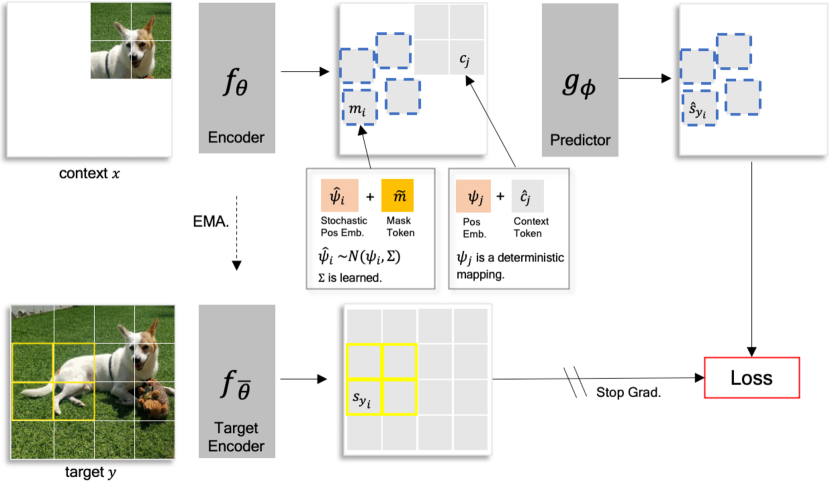
Figure 2: FlexPredict architecture. The model predictor $g_{\psi}$ predicts a target block given masked tokens with stochastic positions and the context representation (obtain via $f_{\theta}$). The objective is to minimize the error between the predicted features and the target features obtained via target encoder $f_{\bar{\theta}}$

Our work leverages the I-JEPA framework [1], which we introduce by outlining its key concept. Specifically, I-JEPA is designed to predict the features of target blocks, based on contextual blocks from the same image. We proceed to elaborate on this in more detail.

Patchification.

Given an image, the standard tokenization process presented at [17] is applied. Specifically, given an input image $I_{x}\in\mathbb{R}^{H\times W\times 3}$, it is first patchified into a sequence of non-overlapping image patches $\hat{p}=(\hat{p}_{1},...,\hat{p}_{k})$ where $\hat{p}_{i}\in\mathbb{R}^{H^{\prime}\times W^{\prime}\times 3}$ and $K=\frac{HW}{H^{\prime}W^{\prime}}$ is the number of patches. Then, each patch is projected to $\mathbb{R}^{d_{e}}$ through a linear fully connected layer. Next, for every patch $\hat{p}_{i}$ the positional embedding features of the $i^{th}$ token are added to it, resulting in the patchfied set $p=\{p_{1},...p_{K}\}$.

Context encoding.

Let $x=\{p_{i}|i\in B_{x}\}$ be the set of context patches where $B_{x}$ denotes the set of context indices. The set of context tokens is randomly chosen as in [1]. First, the context tokens are processed via an encoder model $f_{\theta}$ to obtain deep representations:

$${s}_{x}=f_{\phi}(x)$$

Where $s_{x_{i}}\in\mathbb{R}^{d_{e}}$ is the $i^{th}$ context token representation.

Prediction and loss.

First, a target block of patches is randomly chosen (e.g, tokens annotated in yellow in Figure 2). We denote its corresponding patch indices by $B_{y}$. Next, we define $m=\{\psi_{j}+\tilde{m}\}_{j\in B_{y}}$ to be the set of masked tokens, where for each $j\in B_{y}$, token $m_{j}$ is a summation of a learned masked token $\tilde{m}$, shared across all tokens, and a positional embedding $\psi_{j}$. The predictor $g$ is then used to map from the context tokens and masked tokens to the predicted tokens: $\hat{s}_{y}=g(s_{x},m)$.

To supervise the prediction, $s_{y}=\{s_{y_{i}}\}_{i\in B_{y}}$ is obtained by feeding the patchified image tokens $p$ into a target encoder $f_{\bar{\theta}}$, then selecting the tokens corresponding to $B_{y}$. Finally, the loss is the mean squared error between $s_{y}$ and the predicted tokens $\hat{s}_{y}$:

$$\frac{1}{\lvert B_{y}\rvert}\sum_{i\in B_{y}}\|s_{y_{i}}-\hat{s}_{y_{i}}\|$$ (1)

Here $s_{y}$ is taken as constant, and the parameters of the target encoder $f_{\bar{\theta}}$ are updated via an exponential moving average of the context encoder $f_{{\theta}}$ which has shown to prevent collapse [9, 22].

4 FlexPredict

The I-JEPA method and other MIM-like approaches condition the predictor model on the locations of the target patches, given by the masked tokens positional embeddings, and train the model to predict their content (either in pixel or latent space). This approach does not take into account that the exact location of objects is highly stochastic.

Instead, we force our model to be more flexible in representing locations by conditioning our model on stochastic positions, such that it is impossible to provide a location-accurate prediction. Hence, we refer to our approach as FlexPredict. A high-level schematic view of the model is included in Figure 2.

In what follows, we will explore the process of replacing the positional embeddings of the masked tokens with a stochastic alternative. This involves a few crucial steps, including defining the distribution of the stochastic positions, parameterizing it appropriately, and implementing measures to prevent the model from reducing the impact of the noise to the point where it becomes negligible.

Stochastic Position Embeddings.

In most Visual Transformer implementations, the position of a patch $i$ is encoded via an embedding vector $\psi_{i}$. A common choice is to map the position to sine and cosine features in different frequencies [41, 17]. Here we wish to replace this fixed, deterministic mapping with a stochastic map. This is contrary to past works that use a deterministic mapping to determine the positional embedding of a token [1, 24].

Given a position $i$, we denote by $\hat{\psi}_{i}$ the random variable providing the position embedding. We assume:

$$\hat{\psi}_{i}\sim N(\psi_{i},\Sigma)$$ (2)

Namely, $\hat{\psi}$ is distributed as Gaussian whose mean is the fixed embedding $\psi_{i}$, and covariance matrix $\Sigma\in\mathbb{R}^{d_{p}\times d_{p}}$.

Naturally, we want to learn an optimal $\Sigma$. However, this is challenging for two reasons. First, learning might result in the optimization process setting the values of $\Sigma$ to zero, leading to no randomness. We refer to this case as a “shortcut solution”. Second, the sampling process of $\hat{\psi}$ is non-differential, and therefore we cannot derive gradients to directly optimize it with SGD.

To solve these issues, we start by paramertizing $\Sigma$, then describe how to avoid the “shortcut solution”, and the reparametrization trick to derive a differential algorithm. We start by parameterizing $\Sigma$, and use a general formulation of a low-rank covariance matrix:

$$\Sigma=\sigma AA^{T}$$

Where $A\in\mathbb{R}^{d_{p}\times d_{e}}$ is a learned matrix and $\sigma\in\mathbb{R^{+}}$ is a positive predefined scalar (hyperparameter). By learning matrix $A$, this formulation is flexibile enough, e.g, it is possible learning to assign small variance to low-res location features, while assigning higher variance to higher-frequency features, and also capturing correlations between location features.

Avoiding “shortcuts”.

Without posing any constraints on $A$, it is easy for the model to scale down the noise by setting $A=0$ and making the prediction problem deterministic again, and thereby easier. This would collapse back to the standard I-JEPA model, and lose the advantage of noisy spatial predictions. To avoid this shortcut, we use the following simple trick. We use the matrix $A$ to linearly project every context token $s_{x_{i}}$ as follows: $\hat{c}_{i}=As_{x_{i}}+b$, where $b$ is a learned bias. With this simple trick, it is easy to see that setting $A$ to zero would set the context tokens to zero as well, making the prediction task too difficult for the network and successfully avoiding the above shortcut. This can also be viewed as a regularization of $A$, and we discuss this further in Section 7.

Reparametrization Trick.

Since $\hat{\psi}$ is sampled from a parameterized distribution, it isn’t immediately clear how to optimize over the learned parameters of the distribution $A$, because the sampling operation is non-differentiable in $A$. However, a standard trick in these cases is to reparameterize the distribution so that only sampling is from a fixed distribution that does not depend on $A$ (e.g., see [29]). Specifically, we generate samples from $\hat{\psi}$ by first sampling a vector $n_{i}\in\mathbb{R}^{d_{e}}$ from a standard Gaussian distribution: $n_{i}\sim N(0,\sigma I)$. Then we set $\hat{\psi}$ to the following function:

$$\hat{\psi}_{i}=An_{i}+\psi_{i}$$

The resulting distribution of $\hat{\psi}$ is equal to that in Equation 2, however, we can now differentiate directly through $A$.

Prediction and loss.

Finally, for every $i\in B_{x}$ and $j\in B_{y}$, we define the set of context and masked tokens to be:

$$c_{i}=\psi_{i}+\hat{c}_{i}$$

$$m_{i}=\hat{\psi}_{i}+\tilde{m}$$

Note that here the masked token $m_{i}$ has a stochastic position, and $\tilde{m}$ is a learned bias shared across all positions. We can then apply $g$ to predict the target features $\hat{s}_{y}=g(c,m)$ and use the same loss as in Equation 1.

Algorithm 1 FlexPredict pseudo-code

1:Input: num iterations $K$, image dist $S$, hyperparam $\sigma$,

2:params ${A,b,\tilde{m}}$, encoder $f_{\theta}$, target-encoder $f_{\bar{\theta}}$, predictor $g_{\phi}$, scalar $q$

3:Initialize: $\bar{\theta}=\theta$

4:for $i=1,2,...,K$ do

5:    # sample image mini-batch, apply mask, and encode

6:    $I_{x}\sim S$

7:    $x,y\leftarrow\text{context\_target\_mask}(I_{x})$

8:    $s_{x},s_{y}\leftarrow f_{\theta}(x),f_{\bar{\theta}}(y)$

9:    # apply FlexPredict

10:    $n\sim\mathcal{N}(0,\sigma I)$

11:    $m=An+\psi_{masked}+\tilde{m}$

12:    $c=As_{x}+b+\psi_{context}$

13:    # predict targets and compute loss

14:    $\hat{s}_{y}\leftarrow g_{\phi}(c,m)$

15:    $\text{loss}\leftarrow||\hat{s}_{y}-{s_{y}}\text{\scriptsize.detach()}||_{2}^{2}$

16:    # perform sgd step and update ${\bar{\theta}}$ via ema

17:    $\text{sgd\_step}(\text{loss};\{\theta,\phi,A,b,\tilde{m}\})$

18:    $\bar{\theta}=q{\bar{\theta}}+(1-q)\theta.\text{\scriptsize detach()}$

19:end for

Optimal Predictor.

Our approach relies on using stochastic positional embeddings. Here we provide further analysis of this prediction setting and show that the optimal prediction is indeed to perform spatial smoothing.

Consider a random variable $X$ (corresponding to the context in our case. For simplicity assume $X$ is just the positional embedding of the context) that is used to predict a variable $Y$ (corresponding to the target in our case). But now instead of predicting from $X$, we use a noise variable $Z$ that is independent of both $X,Y$, and provide the predictor with only the noisy result $R=g(X,Z)$. Here $g$ is some mixing function (in our case $g(x,z)=x+z$). We next derive the optimal predictor $f(R)$ in this case. Formally we want to minimize:

$$E_{R,Y}[(f(R)-Y)^{2}]$$ (3)

A classic result in estimation is that this is optimized by the conditional expectation $f(r)=E[Y|R=r]$. We simplify this as follows:

$$E[Y|R=r] = \sum_{x,y}yp(Y=y,X=x|R=r)$$

$$= \sum_{x,y}yp(y|X=x)p(X=x|R=r)$$

$$= \sum_{x}E[Y|X=x]p(X=x|R=r)$$

where in the second line we used the fact that:

$$p(y,x|r)=p(y|x,r)p(x|r)=p(y|x)p(x|r)$$ (4)

To further illustrate, consider the case where $z$ is Gaussian with zero mean and unit variance. Then $p(x|r)$ is also Gaussian with expectation $r$, and the expression above amounts to convolution of the clean expected values with a Gaussian:

$$\int_{x}E[Y|X=x]\frac{1}{\sqrt{2\pi}}e^{-0.5(x-r)^{2}}dx$$ (5)

5 Experiments

Next, we turn to discuss the main experiments presented in the paper. We start by discussing the ablation study and design choices in Section 5.1. Then in Section 5.2, we describe the application of FlexPredict to various downstream tasks including image recognition, dense prediction, and low-level vision tasks.

5.1 Ablation study

Our primary focus was to evaluate the effectiveness of adding noise. For this purpose, we experimented with learning $A$ given different hyper-parameter $\sigma$. We also investigated the impact of adding noise from fixed Gaussian distributions, namely $\Sigma=\sigma I$, without learning. Lastly, we evaluate the effect of applying FlexPredict to context and/or masked tokens positions.

We evaluated various design options for the FlexPredict model. For each setting, we implemented the encoder and predictor using ViT-B architecture and pre-trained them for $300$ epochs on IN-1k. We then assessed the linear probing performance on IN-1k using only 1% of the available labels.

5.2 Downstream Tasks

We conducted pre-training of the FlexPredict model on IN-1k for a period of $600$ epochs, utilizing either ViT-B or ViT-L architectures for the encoder and predictor. Subsequently, we proceeded to evaluate the model’s performance on a variety of downstream tasks. We include the full implementation details in the Supplementary Material.

Following past works, we focus on evaluating the (target) encoder representations [24, 1], and use the standard VISSL [21] evaluation protocol like in [1].

Image recognition.

For image classification, we evaluated the FlexPredict model linear probing performance on multiple datasets, including ImageNet (IN-1k) [37], Places 205 [51], iNaturalist 2018 [40], and CIFAR 100 [30]. These datasets vary in their size, their purpose, and the geographical environments from which the images were captured. For example, IN-1k contains over $1.2$ million images compared to CIFAR-100 which contains only $60,000$ images, and while IN-1k is focused on object recognition, Places is focused on scene recognition.

Dense prediction.

To evaluate how well FlexPredict performs on dense prediction tasks, e.g, tasks that require fine-grained spatial representations, we utilized the learned model for semi-supervised video object segmentation on the DAVIS 2017 [36] dataset. We follow previous works (e.g [27, 9]) and use the pretrained FlexPredict to extract frames features and use patch-level affinities between frames to propagate the first segmentation mask.

Low-level vision.

We assessed the linear probing performance of our model on downstream tasks related to low-level vision. These tasks included object counting and object ordering by depth, which were evaluated using the CLEVR [28] dataset. In order to accurately perform these tasks, the model needed to not only recognize objects but also capture their location features.

6 Results

We report the ablation study results in Section 6.1, then discuss results on various downstream tasks in Section 6.2.

6.1 Ablations

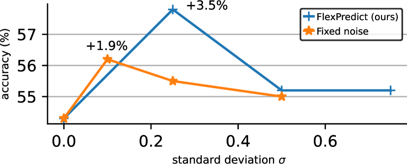
Figure 3: Using stochastic positional embeddings. sampling from distribution with learned covariance matrix as in FlexPredict, e.g, $\Sigma=\sigma AA^{T}$ leads to $+3.5\%$ improvement, while using a fixed covariance matrix $\Sigma=\sigma I$ leads to smaller $1.9\%$ improvement. Accuracy is based on probing using 1% of the data from IN-1k.

Method	Top-1
No Noise (I-JEPA [1])	54.3
Context tokens only	55.1
Masked tokens only	fbApp57.8
Masked + context tokens	56.8

Table 1: Applying noise to different tokens. Applying learned noise to context and/or masked tokens positional embeddings. Accuracy is based on linear probing using 1% of the data from IN-1k.

We present the results comparing different noise, and the impact when changing the hyperparam $\sigma$. Figure 3 indicates that it is optimal to learn the parameters of the distribution as in FlexPredict, rather than use fixed parameters. Our findings demonstrate that setting $\sigma=0.25$ leads to an improvement of $3.5\%$ points compared to I-JEPA. Additionally, Table 1 reveals that FlexPredict is most beneficial when applied solely to masked tokens positional embeddings, not to context.

6.2 Downstream Tasks

Next, we report the downstream performance of FlexPredict on image recognition, dense prediction, and low-level vision tasks.

Image recognition.

In Table 2, we present the linear probing image classification results conducted on IN-1k. Our approach, FlexPredict, achieves a performance improvement of $1.6\%$ and $0.9\%$ when using ViT-B and ViT-L, respectively, compared to previous MIM methods. Additionally, FlexPredict narrows the relative performance gap from iBOT [53] by 25%. Furthermore, our approach outperforms existing methods in downstream linear probing tasks. For example, FlexPredict leads to over 10% improvement on CIFAR-100 using ViT-B and 1% using ViT-L. This confirms that the learned representations lead to improvements in a large variety of image recognition tasks.

Method	Arch.	Epochs	Top-1
MIM methods, without view data augmentations
data2vec [3]	ViT-L/16	1600	53.5
MAE [24]	ViT-B/16	1600	68.0
	ViT-L/16	1600	76.0
I-JEPA [1]	ViT-B/16	600	72.9
	ViT-L/16	600	77.5
FlexPredict	fbAppViT-B/16	fbApp600	fbApp74.5
	fbAppViT-L/16	fbApp600	fbApp78.4
Invariance-based methods, using extra view data augmentations
SimCLR v2 [11]	RN152 ($2\times$)	800	79.1
DINO [9]	ViT-B/16	400	78.1
MoCo v3 [14]	ViT-B/16	300	76.7
iBOT [53]	ViT-B/16	250	79.8
	ViT-L/16	250	81.0

Table 2: Linear-evaluation on IN-1k. FlexPredict improves linear probing performance compared to other methods that do not rely on hand-crafted view data-augmentations during pretraining.

Method	Arch.	CIFAR100	Places205	iNat18
MIM methods, without view data augmentations
data2vec [3]	ViT-L/16	59.6	36.9	10.9
MAE [24]	ViT-B/16	68.1	49.2	26.8
	ViT-L/16	77.4	54.4	33.0
I-JEPA [1]	ViT-B/16	69.2	53.4	43.4
	ViT-L/16	83.6	56.5	48.4
FlexPredict	fbAppViT-B/16	fbApp81.2	fbApp54.3	fbApp44.7
	fbAppViT-L/16	fbApp84.7	fbApp57.2	fbApp49.2
Invariance-based methods, using extra view data augmentations
DINO [9]	ViT-B/16	84.8	55.2	50.1
iBOT [53]	ViT-B/16	85.5	56.7	50.0
	ViT-L/16	88.3	60.4	57.3

Table 3: Linear-probe transfer for image classification. Linear-evaluation on downstream image classification tasks. FlexPredict significantly outperforms previous methods that also do not use augmentations (MAE and data2vec), and decreases the gap with the best view-invariance-based methods that leverage hand-crafted data augmentations during pretraining.

Method	Arch.	J-Mean	F-Mean	J&F Mean
MIM methods, without view data augmentations
MAE [24]	ViT-B/16	49.4	52.6	50.9
	ViT-L/16	52.5	54.3	53.4
I-JEPA [1]	ViT-B/16	56.1	56.2	56.1
	ViT-L/16	56.1	55.7	55.9
FlexPredict	fbAppViT-B/16	fbApp56.6	fbApp57.3	fbApp57.0
	fbAppViT-L/16	fbApp58.1	fbApp58.7	fbApp58.4
Invariance-based methods, using extra view data augmentations
DINO [9]	ViT-B/16	60.7	63.9	62.3
iBOT [53]	ViT-B/16	60.9	63.3	62.1
	ViT-L/16	61.7	63.9	62.8

Table 4: Video objects semi-supervised segmentation. The results demonstrate that compared to MIM baselines, FlexPredict learns features in a finer level of granularity. Results reported on the DAVIS 2017 [36] dataset.

Method	Arch.	Clevr/Count	Clevr/Dist
MIM methods, without view data augmentations
data2vec [3]	ViT-L/16	72.7	53.0
MAE [24]	ViT-B/16	86.6	70.8
	ViT-L/16	92.1	73.0
I-JEPA [1]	ViT-B/16	82.2	70.7
	ViT-L/16	85.6	71.2
FlexPredict	fbAppViT-B/16	fbApp83.7	fbApp71.3
	fbAppViT-L/16	fbApp85.7	fbApp70.2
Invariance-based methods, using extra view data augmentations
DINO [9]	ViT-B/16	83.2	62.5
iBOT [53]	ViT-B/16	85.1	64.4
	ViT-L/16	85.7	62.8

Table 5: Linear-probing on low-level vision downstream tasks like object counting (CLEVR/Count) and depth prediction (Clevr/Dist). FlexPredict effectively captures low-level location features and it is on par or better than I-JEPA.

Dense prediction.

We include semi-supervised video-object segmentation results in Table 4. We find that FlexPredict significantly improves over I-JEPA [1], e.g, an improvement of $2.5\%$ on $J\&F$ using ViT-L. Notably, we find that while using I-JEPA does not lead to improvements here by scaling the model, scaling the model to ViT-L leads to a $1.4\%$ improvement compared to ViT-B using FlexPredict.

Low-level vision.

Table 5 provides evidence that the learned representations of FlexPredict performs at least on-par with I-JEPA models in low-level tasks such as counting and depth ordering on the CLEVR dataset.

7 Analysis

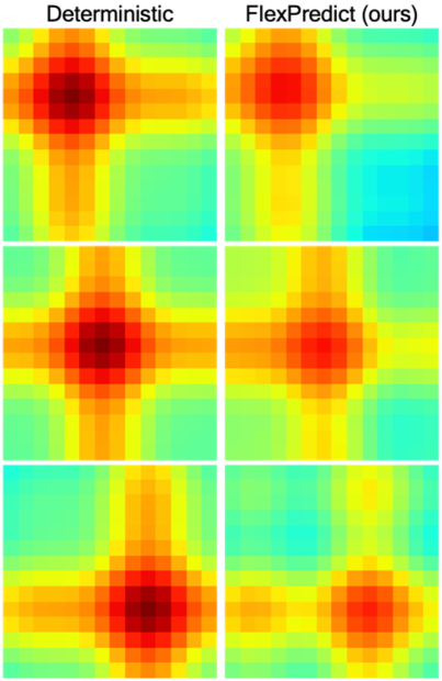
Figure 4: Similarity matrices of positional embeddings matrix between deterministic ($\psi\psi_{i}$) and stochastic FlexPredict ($\psi\hat{\psi}_{i}$) positions. Each row represents a different target position $i$. Position embeddings are based on sine and cosine features.

We perform a thorough analysis of FlexPredict. Specifically, we examine the stochastic effect of FlexPredict and attempt to interpret the properties of the learned model.

Regularization.

We train FlexPredict models, changing only the hyperparam $\sigma$. We find that increasing the value of $\sigma$ leads to a decrease in the norm of $A$, which can be viewed as regularization. On the other hand, increasing $\sigma$ leads to an increase in the norm of the masked token $m$. The mask token scale increases to prevent losing its information relative to the noise. We show this dynamic in Figure 5.

Regularized I-JEPA.

Based on the observations above, we train additional models to check whether FlexPredict can be explained by regularization. Specifically, we train I-JEPA models while applying $l_{1}$ regularization on the predictor’s linear projection layer weights. We evaluate linear probing performance using $1\%$ of the labels and find this leads to $1.5\%$ improvement over I-JEPA, compared to $3.5\%$ improvement using FlexPredict.

Stochastic positional embeddings visualization.

In order to visualize stochastic positional embeddings, we sampled stochastic positions and generated a similarity matrix of each sample with the predefined deterministic positions. Figure 4 provides examples of this. Our findings show that when noise is added to a positional embedding, the resulting similarity matrix changes, which makes it similar to a wider range of neighboring locations.

Low-res prediction.

We build on the observations above and train additional I-JEPA models to investigate if FlexPredict performance could be achieved through predicting lower-scale features. We trained models to predict features in both the original scale and a downscaled version by a factor of 2, using bilinear resizing and max pooling for downscaling. However, we found that these methods did not significantly improve performance, as reported in Table 6.

Predictions visualization.

We include heatmap visualization to visualize the similarity of a predicted token to all other tokens within the same image (see Figure 6). For a given image, mask, and a masked patch of interest, we apply cosine similarity between the predicted patch and all other token representations within the same image (given by the target encoder), followed by a softmax. For I-JEPA the visualization indicates that adjacent tokens tend to share similar features, implying a correlation between the features and spatial location. In contrast, FlexPredict produces predictions correlated with non-neighboring small areas. We speculate that training with stochastic positions prevents spatial adjacency bias.

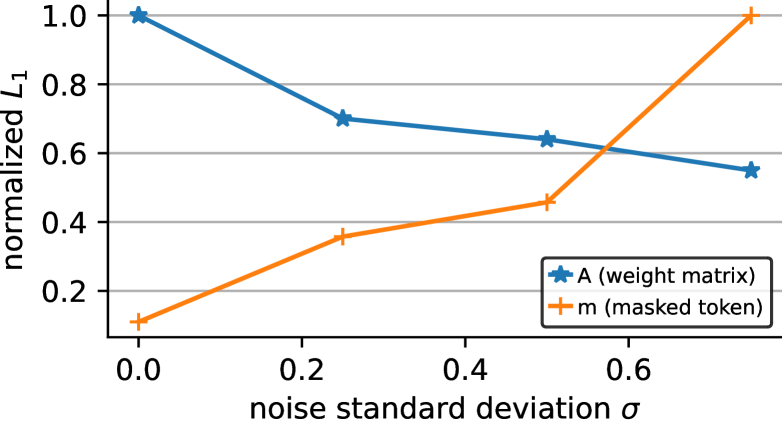
Figure 5: Increasing $\sigma$ induces regularization. The effect of changing the hyperparameter $\sigma$ on the norm of learned parameter $A$ and the masked token $m$. As we increase $\sigma$, the norm of $A$ decreases, indicating regularization. However, the norm of the masked token increases, likely to preserve its information relative to the added noise.

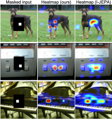
Figure 6: Predicted features visualization. We show a similarity heatmap between the predicted features of a given patch (marked in white within the masked area) and the other tokens encoded by the target encoder in the same image. For I-JEPA, adjacent tokens tend to share similar features, implying a correlation between the features and spatial location. In contrast, FlexPredict produces predictions correlated with non-neighboring small areas. We speculate that FlexPredict reduces spatial adjacency bias.

Method	Top-1
I-JEPA [1])	54.3
Low res pred (bilinear resize)	52.1
Low res (max pooling)	54.1
FlexPredict	fbApp57.8

Table 6: Low resolution prediction. We evaluated the performance of FlexPredict against models that predict features on the original scale and an $x2$ downscaled version using either max pooling or bilinear resizing. Reporting linear evaluation results on IN-1K using only 1% of the labels

8 Conclusion

In this work, we proposed FlexPredict, a stochastic model that tackles location uncertainties in the MIM task. By conditioning on stochastic masked tokens positions, our model learns features that are more robust to location uncertainties. The effectiveness of this approach is demonstrated on various datasets and downstream tasks, outperforming existing MIM methods and highlighting its potential for self-supervised learning. We speculate, based on our experiments and visualizations, that by modeling location uncertainties, FlexPredict suffers less from spatial adjacency bias. Other sources of uncertainty, like uncertainty in appearance, require further investigation in future work.

Acknowledgments:

AG’s group has received funding from the European Research Council (ERC) under the European Unions Horizon 2020 research and innovation programme (grant ERC HOLI 819080). TD’s group was funded by DoD including DARPA LwLL and the Berkeley AI Research (BAIR) Commons. This work was completed in partial fulfillment for the Ph.D degree of the first author.

Appendix

Appendix A Implementation Details

We include the full implementation details, pretraining configs and evaluation protocols for the Ablations (see Appendix A.1) and Downstream Tasks (Appendix A.2).

A.1 Ablations

Here we pretrain all models for $300$ epochs using $4$ V100 nodes, on a total batch size of $2048$. In all the ablation study experiments, we follow the recipe of [1]. We include the full config in Table 7.

To evaluate the pretrained models, we use linear probing evaluation using 1% of IN-1k [37]. To obtain the features of an image, we apply the target encoder over the image to obtain a sequence of tokens corresponding to the image. We then average the tokens to obtain a single representative vector. The linear classifier is trained over this representation, maintaining the rest of the target encoder layers fixed.

A.2 Downstream Tasks

Here we pretrain FlexPredict for $600$ epochs using $4$ V100 nodes, on a total batch size of $2048$ using ViT-B (see config in Table 8) and ViT-L (see config in Table 9). We follow a similar config compared to [1] except we use a lower learning rate. Intuitively, since FlexPredict is stochastic it is more sensitive to high learning rates.

For evaluation on downstream tasks, we use the features learned by the target-encoder and follow the protocol of VISSL [21] that was utilized by I-JEPA [1]. Specifically, we report the best linear evaluation number among the average-pooled patch representation of the last layer and the concatenation of the last $4$ layers of the average-pooled patch representations.

For baselines that use Vision Transformers [17] with a [cls] token (e.g, iBOT [53], DINO [9] or MAE [24]), we use the default configurations of VISSL [21] to evaluate the publicly available checkpoints on iNaturalist18 [40], CIFAR100 [31], Clevr/Count [28, 49], Clevr/Dist [28, 49], and Places205 [52]. Following the evaluation protocol of VISSL [21], we freeze the encoder and return the best number among the [cls] token representation of the last layer and the concatenation of the last $4$ layers of the [cls] token.

For semi-supervised video object segmentation, we propagate the first labeled frame in a video using the similarity between adjacent frames features. To label the video using the frozen features, we follow the code and hyperparams of [9]. To evaluate the segmented videos, we use the evaluation code of DAVIS 2017 [36].

config	value
optimizer	AdamW
epochs	300
learning rate	$1e^{-3}$
weight decay	$(0.04,0.4)$
batch size	2048
learning rate schedule	cosine decay
warmup epochs	15
encoder arch.	ViT-B
predicted targets	4
predictor depth	6
predictor attention heads	12
predictor embedding dim.	384
$\sigma$ (noise hyperparam)	$0.25$

Table 7: Pretraining setting for ablations. Using ViT-B encoder, trained for $300$ epochs, config strictly follows [1].

config	value
optimizer	AdamW
epochs	$600$
learning rate	$8e^{-4}$
weight decay	$(0.04,0.4)$
batch size	$2048$
learning rate schedule	cosine decay
warmup epochs	15
encoder arch.	ViT-B
predicted targets	4
predictor depth	6
predictor attention heads	12
predictor embedding dim.	384
$\sigma$ (noise hyperparam)	$0.25$

Table 8: Pretraining setting for downstream tasks (ViT-B). All models trained for $600$ epochs.

config	value
optimizer	AdamW
epochs	$600$
learning rate	$8e^{-4}$
weight decay	$(0.04,0.4)$
batch size	$2048$
learning rate schedule	cosine decay
warmup epochs	15
encoder arch.	ViT-L
predicted targets	4
predictor depth	12
predictor attention heads	16
predictor embedding dim.	384
$\sigma$ (noise hyperparam)	$0.25$

Table 9: Pretraining setting for downstream tasks (ViT-L). All models trained for $600$ epochs.

References

- [1] Mahmoud Assran, Quentin Duval, Ishan Misra, Piotr Bojanowski, Pascal Vincent, Michael Rabbat, Yann LeCun, and Nicolas Ballas. Self-supervised learning from images with a joint-embedding predictive architecture. arXiv preprint arXiv:2301.08243, 2023.
- [2] Alexei Baevski, Wei-Ning Hsu, Alexis Conneau, and Michael Auli. Unsupervised speech recognition. Advances in Neural Information Processing Systems, 34:27826–27839, 2021.
- [3] Alexei Baevski, Wei-Ning Hsu, Qiantong Xu, Arun Babu, Jiatao Gu, and Michael Auli. Data2vec: A general framework for self-supervised learning in speech, vision and language. arXiv preprint arXiv:2202.03555, 2022.
- [4] Alexei Baevski, Yuhao Zhou, Abdelrahman Mohamed, and Michael Auli. wav2vec 2.0: A framework for self-supervised learning of speech representations. Advances in neural information processing systems, 33:12449–12460, 2020.
- [5] Hangbo Bao, Li Dong, and Furu Wei. Beit: Bert pre-training of image transformers. arXiv preprint arXiv:2106.08254, 2021.
- [6] Adrien Bardes, Jean Ponce, and Yann LeCun. Vicreg: Variance-invariance-covariance regularization for self-supervised learning. arXiv preprint arXiv:2105.04906, 2021.
- [7] Adrien Bardes, Jean Ponce, and Yann LeCun. Vicregl: Self-supervised learning of local visual features. arXiv preprint arXiv:2210.01571, 2022.
- [8] Tom Brown, Benjamin Mann, Nick Ryder, Melanie Subbiah, Jared D Kaplan, Prafulla Dhariwal, Arvind Neelakantan, Pranav Shyam, Girish Sastry, Amanda Askell, et al. Language models are few-shot learners. Advances in neural information processing systems, 33:1877–1901, 2020.
- [9] Mathilde Caron, Hugo Touvron, Ishan Misra, Hervé Jégou, Julien Mairal, Piotr Bojanowski, and Armand Joulin. Emerging properties in self-supervised vision transformers. arXiv preprint arXiv:2104.14294, 2021.
- [10] Ting Chen, Simon Kornblith, Mohammad Norouzi, and Geoffrey Hinton. A simple framework for contrastive learning of visual representations. preprint arXiv:2002.05709, 2020.
- [11] Ting Chen, Simon Kornblith, Kevin Swersky, Mohammad Norouzi, and Geoffrey Hinton. Big self-supervised models are strong semi-supervised learners. arXiv preprint arXiv:2006.10029, 2020.
- [12] Xinlei Chen, Haoqi Fan, Ross Girshick, and Kaiming He. Improved baselines with momentum contrastive learning. arXiv preprint arXiv:2003.04297, 2020.
- [13] Xinlei Chen and Kaiming He. Exploring simple siamese representation learning. In Proceedings of the IEEE/CVF conference on computer vision and pattern recognition, pages 15750–15758, 2021.
- [14] Xinlei Chen, Saining Xie, and Kaiming He. An empirical study of training self-supervised vision transformers. arXiv preprint arXiv:2104.02057, 2021.
- [15] Kevin Clark, Minh-Thang Luong, Quoc V Le, and Christopher D Manning. Electra: Pre-training text encoders as discriminators rather than generators. arXiv preprint arXiv:2003.10555, 2020.
- [16] Jacob Devlin, Ming-Wei Chang, Kenton Lee, and Kristina Toutanova. Bert: Pre-training of deep bidirectional transformers for language understanding. arXiv preprint arXiv:1810.04805, 2018.
- [17] Alexey Dosovitskiy, Lucas Beyer, Alexander Kolesnikov, Dirk Weissenborn, Xiaohua Zhai, Thomas Unterthiner, Mostafa Dehghani, Matthias Minderer, Georg Heigold, Sylvain Gelly, et al. An image is worth 16x16 words: Transformers for image recognition at scale. arXiv preprint arXiv:2010.11929, 2020.
- [18] Alexey Dosovitskiy, Jost Tobias Springenberg, Martin A. Riedmiller, and Thomas Brox. Discriminative unsupervised feature learning with convolutional neural networks. In NIPS, 2014.
- [19] Debidatta Dwibedi, Yusuf Aytar, Jonathan Tompson, Pierre Sermanet, and Andrew Zisserman. With a little help from my friends: Nearest-neighbor contrastive learning of visual representations. In Proceedings of the IEEE/CVF International Conference on Computer Vision, pages 9588–9597, 2021.
- [20] Aleksandr Ermolov, Aliaksandr Siarohin, E. Sangineto, and N. Sebe. Whitening for self-supervised representation learning. In International Conference on Machine Learning, 2020.
- [21] Priya Goyal, Quentin Duval, Jeremy Reizenstein, Matthew Leavitt, Min Xu, Benjamin Lefaudeux, Mannat Singh, Vinicius Reis, Mathilde Caron, Piotr Bojanowski, Armand Joulin, and Ishan Misra. Vissl. https://github.com/facebookresearch/vissl, 2021.
- [22] Jean-Bastien Grill, Florian Strub, Florent Altché, Corentin Tallec, Pierre H Richemond, Elena Buchatskaya, Carl Doersch, Bernardo Avila Pires, Zhaohan Daniel Guo, Mohammad Gheshlaghi Azar, et al. Bootstrap your own latent: A new approach to self-supervised learning. arXiv preprint arXiv:2006.07733, 2020.
- [23] Raia Hadsell, Sumit Chopra, and Yann LeCun. Dimensionality reduction by learning an invariant mapping. 2006 IEEE Computer Society Conference on Computer Vision and Pattern Recognition (CVPR’06), 2:1735–1742, 2006.
- [24] Kaiming He, Xinlei Chen, Saining Xie, Yanghao Li, Piotr Dollár, and Ross Girshick. Masked autoencoders are scalable vision learners. arXiv preprint arXiv:2111.06377, 2021.
- [25] Kaiming He, Haoqi Fan, Yuxin Wu, Saining Xie, and Ross Girshick. Momentum contrast for unsupervised visual representation learning. arXiv preprint arXiv:1911.05722, 2019.
- [26] Tianyu Hua, Wenxiao Wang, Zihui Xue, Sucheng Ren, Yue Wang, and Hang Zhao. On feature decorrelation in self-supervised learning. In Proceedings of the IEEE/CVF International Conference on Computer Vision (ICCV), pages 9598–9608, October 2021.
- [27] Allan Jabri, Andrew Owens, and Alexei Efros. Space-time correspondence as a contrastive random walk. Advances in neural information processing systems, 33:19545–19560, 2020.
- [28] Justin Johnson, Bharath Hariharan, Laurens Van Der Maaten, Li Fei-Fei, C Lawrence Zitnick, and Ross Girshick. Clevr: A diagnostic dataset for compositional language and elementary visual reasoning. In Proceedings of the IEEE conference on computer vision and pattern recognition, pages 2901–2910, 2017.
- [29] Diederik P Kingma and Max Welling. Auto-encoding variational bayes. arXiv preprint arXiv:1312.6114, 2013.
- [30] Alex Krizhevsky. Learning multiple layers of features from tiny images. Technical report, 2009.
- [31] Alex Krizhevsky, Geoffrey Hinton, et al. Learning multiple layers of features from tiny images. 2009.
- [32] Yann LeCun. A path towards autonomous machine intelligence version 0.9. 2, 2022-06-27. 2022.
- [33] Ishan Misra and Laurens van der Maaten. Self-supervised learning of pretext-invariant representations. In Proceedings of the IEEE Conference on Computer Vision and Pattern Recognition, pages 6707–6717, 2020.
- [34] Aaron van den Oord, Yazhe Li, and Oriol Vinyals. Representation learning with contrastive predictive coding. arXiv preprint arXiv:1807.03748, 2018.
- [35] Deepak Pathak, Philipp Krahenbuhl, Jeff Donahue, Trevor Darrell, and Alexei A Efros. Context encoders: Feature learning by inpainting. In Proceedings of the IEEE conference on computer vision and pattern recognition, pages 2536–2544, 2016.
- [36] Jordi Pont-Tuset, Federico Perazzi, Sergi Caelles, Pablo Arbeláez, Alex Sorkine-Hornung, and Luc Van Gool. The 2017 davis challenge on video object segmentation. arXiv preprint arXiv:1704.00675, 2017.
- [37] Olga Russakovsky, Jia Deng, Hao Su, Jonathan Krause, Sanjeev Satheesh, Sean Ma, Zhiheng Huang, Andrej Karpathy, Aditya Khosla, Michael Bernstein, Alexander C. Berg, and Li Fei-Fei. Imagenet large scale visual recognition challenge. International Journal of Computer Vision, 115(3):211–252, 2015.
- [38] Ruslan Salakhutdinov and Geoff Hinton. Learning a nonlinear embedding by preserving class neighbourhood structure. In Artificial Intelligence and Statistics, pages 412–419. PMLR, 2007.
- [39] Yonglong Tian, Dilip Krishnan, and Phillip Isola. Contrastive multiview coding. In European Conference on Computer Vision, 2019.
- [40] Grant Van Horn, Oisin Mac Aodha, Yang Song, Yin Cui, Chen Sun, Alex Shepard, Hartwig Adam, Pietro Perona, and Serge Belongie. The inaturalist species classification and detection dataset. In Proceedings of the IEEE conference on computer vision and pattern recognition, pages 8769–8778, 2018.
- [41] Ashish Vaswani, Noam Shazeer, Niki Parmar, Jakob Uszkoreit, Llion Jones, Aidan N Gomez, Łukasz Kaiser, and Illia Polosukhin. Attention is all you need. In Advances in neural information processing systems, pages 5998–6008, 2017.
- [42] Pascal Vincent, Hugo Larochelle, Yoshua Bengio, and Pierre-Antoine Manzagol. Extracting and composing robust features with denoising autoencoders. In Proceedings of the 25th international conference on Machine learning, pages 1096–1103, 2008.
- [43] Pascal Vincent, Hugo Larochelle, Isabelle Lajoie, Yoshua Bengio, Pierre-Antoine Manzagol, and Léon Bottou. Stacked denoising autoencoders: Learning useful representations in a deep network with a local denoising criterion. Journal of machine learning research, 11(12), 2010.
- [44] Weiran Wang, Qingming Tang, and Karen Livescu. Unsupervised pre-training of bidirectional speech encoders via masked reconstruction. In ICASSP 2020-2020 IEEE International Conference on Acoustics, Speech and Signal Processing (ICASSP), pages 6889–6893. IEEE, 2020.
- [45] Zhirong Wu, Yuanjun Xiong, Stella X Yu, and Dahua Lin. Unsupervised feature learning via non-parametric instance discrimination. In Proceedings of the IEEE conference on computer vision and pattern recognition, pages 3733–3742, 2018.
- [46] Tete Xiao, Xiaolong Wang, Alexei A Efros, and Trevor Darrell. What should not be contrastive in contrastive learning. In International Conference on Learning Representations.
- [47] Zhenda Xie, Zheng Zhang, Yue Cao, Yutong Lin, Jianmin Bao, Zhuliang Yao, Qi Dai, and Han Hu. Simmim: A simple framework for masked image modeling. arXiv preprint arXiv:2111.09886, 2021.
- [48] Jure Zbontar, Li Jing, Ishan Misra, Yann LeCun, and Stéphane Deny. Barlow twins: Self-supervised learning via redundancy reduction. arXiv preprint arXiv:2103.03230, 2021.
- [49] Xiaohua Zhai, Joan Puigcerver, Alexander Kolesnikov, Pierre Ruyssen, Carlos Riquelme, Mario Lucic, Josip Djolonga, Andre Susano Pinto, Maxim Neumann, Alexey Dosovitskiy, Lucas Beyer, Olivier Bachem, Michael Tschannen, Marcin Michalski, Olivier Bousquet, Sylvain Gelly, and Neil Houlsby. A large-scale study of representation learning with the visual task adaptation benchmark, 2019.
- [50] Richard Zhang, Phillip Isola, and Alexei A Efros. Colorful image colorization. 2016.
- [51] Bolei Zhou, Agata Lapedriza, Jianxiong Xiao, Antonio Torralba, and Aude Oliva. Learning deep features for scene recognition using places database. In Z. Ghahramani, M. Welling, C. Cortes, N. Lawrence, and K.Q. Weinberger, editors, Advances in Neural Information Processing Systems, volume 27. Curran Associates, Inc., 2014.
- [52] Bolei Zhou, Agata Lapedriza, Jianxiong Xiao, Antonio Torralba, and Aude Oliva. Learning deep features for scene recognition using places database. Advances in neural information processing systems, 27, 2014.
- [53] Jinghao Zhou, Chen Wei, Huiyu Wang, Wei Shen, Cihang Xie, Alan Yuille, and Tao Kong. Ibot: Image bert pre-training with online tokenizer. arXiv preprint arXiv:2111.07832, 2021.