Electrically-programmable frequency comb for compact quantum photonic circuits

Abstract

Recent efforts have demonstrated the first prototypes of compact and programmable photonic quantum computers (PQCs). Utilization of time-bin encoding in loop-like architectures enabled programmable generation of quantum states and execution of different (programmable) logic gates on a single circuit. Actually, there is still space for better compactness and complexity of available quantum states: photonic circuits (PCs) can function at different frequencies. This necessitates an optical component which can make different frequencies talk with each other. This component should be integrable into PCs and be controlled –preferably– by voltage for programmable generation of multifrequency quantum states and PQCs. Here, we propose such a device which controls four-wave mixing process, essential for frequency combs. We utilize nonlinear Fano resonances. Entanglement generated by the device can be tuned continuously by the applied voltage which can be delivered to the device via nm-thick wires. The device is integrable, CMOS-compatible, and operates within a timescale of hundreds of femtoseconds.

I Introduction

Demonstrations of quantum supremacy over classical computers Harrow and Montanaro (2017); Zhong et al. (2020) intensified the research on integrated quantum circuits (IQCs) where generation, processing, and detection of quantum states can be carried out on a single chip Masada et al. (2015); Vaidya et al. (2020). This increased the demand for scalable integration of nonlinear optical components, such as squeezers Mondain et al. (2019); Zhang et al. (2021), frequency combs Kues et al. (2019) and other nonlinearity generators, into IQC chips. Though integration of various nonlinear components into IQCs are demonstrated successfully Pelucchi et al. (2022), nonlinearity (for squeezing and entanglement) generation in such devices are either fixed Zhao et al. (2020) or cannot be tuned conveniently Lu et al. (2021); Hallett et al. (2018); Foster et al. (2019); Wang et al. (2020).

In order to achieve the quantum supremacy on a wider range of computations, it is necessary to build programmable quantum computers (QCs) Madsen et al. (2022); Asavanant et al. (2021); Larsen et al. (2021); Takeda and Furusawa (2017); Arrazola et al. (2021); Enomoto et al. (2021); Arute et al. (2019), in which flexible quantum states can be generated Madsen et al. (2022); Arrazola et al. (2021) and various logic gates can be implemented Takeda and Furusawa (2017); Arrazola et al. (2021); Larsen et al. (2021). In state-of-the-art PQCs, a given initial squeezing (nonclassicality) is supplied to the circuit on the first module and different entangled states are produced via variable beam-splitters (VBSs) and phase-shifters Madsen et al. (2022); Arrazola et al. (2021). In the current PQCs, information is encoded in a pulse train where each pulse corresponds to a mode within the time-domain multiplexing Yokoyama et al. (2013). The pulses (modes) are made interact with each other in a loop-structure in order to obtain several-dimensional entangled states. That is, tunability of, for instance, squeezing is rather a new concept Günay et al. (2023). Computation can also be performed in similar loop-like architectures where different logic gates can be implemented using measurement-induced squeezing protocol with VBSs Takeda and Furusawa (2017); Arrazola et al. (2021); Larsen et al. (2021). A single circuit can execute a universal gate Braunstein and van Loock (2005) by winding the input pulse in that programmable circuit.

Such a loop architecture provides extreme compactness regarding both quantum state preparation and computing. Nevertheless, there is more to do with the compactness and complexity of PQCs Caspani et al. (2016). A given circuit can function at different frequencies Kues et al. (2019). If one can entangle (link) the pulses of different frequencies Mahmudlu et al. (2023), the functionality of the PQCs can be increased tremendously. For this reason, a close attention is paid on scalable (integrated) frequency combs Caspani et al. (2016); Kues et al. (2019, 2017); Mahmudlu et al. (2023). While important achievements are obtained, the fabricated combs are not conveniently (electrically) programmable, yet.

A frequency comb employs, e.g., four-wave mixing (FWM) process, where central (pump) pulse is split into two side bands. The new side bands also yield other side bands, resulting a comb of different frequencies. Thus, if one can control the FWM process, she/he can program the frequency comb.

Figure 1: Control mechanism of programmable frequency comb which introduces configurable links (entanglement) among different frequency modes in an IQC. A PNS is placed in a photonic cavity. The resonance of the QE, positioned at the hotspot of the PNS, is controlled electrically via a voltage applied over the PNS itself. The QE resonance controls the FWM process (see Fig. 3) taking place within the device. Cyclic use of the FWM process generates a frequency comb Kues et al. (2019). Thus, the links among different frequency components can be programmed electrically.

Here, we propose a device where the FWM process can be controlled (continuously tuned) by an applied voltage Shibata et al. (2013); Hallett et al. (2018); Chakraborty et al. (2015); Schwarz et al. (2016) which can be delivered through nm-thick wires. The device is integrable into quantum photonic circuits and CMOS-compatible. A quantum emitter (QE), located at the hot-spot of a plasmonic nanostructure (PNS), introduces a Fano resonance in the nonlinear response Singh et al. (2016); Tasgın et al. (2018), see Figs. 1 and 3. Depending on the QE’s resonance $\Omega_{\rm\scriptscriptstyle QE}$, the FWM process ($\omega_{3}=1.8\omega_{1}$) can either be turned off (at $\Omega_{\rm\scriptscriptstyle QE}=\omega_{3}=1.8000\omega_{1}$) or can be further enhanced (at $\Omega_{\rm\scriptscriptstyle QE}\simeq 1.8005\omega_{1}$) on top of the field-enhanced FWM of the bare nanostructure, see Fig. 3. (Here, $\omega_{1}$ is the pump frequency used in scaling and $\omega_{3}=1.8\omega_{1}$ corresponds to the FWM frequency.)

Fano resonances take place at sharp frequency intervals Postaci et al. (2018); Günay et al. (2020). This may be disadvantageous for broadband enhancement of nonlinearity. However, here it becomes extremely useful for programming the FWM process via a meV-tuning of the QE’s resonance Shibata et al. (2013); Hallett et al. (2018); Chakraborty et al. (2015). One should also note that while plasmonic excitations decay in a few femtoseconds, quantum optics experiments with plasmons Fasel et al. (2005); Tame et al. (2013); Fasel et al. (2006); Huck et al. (2009); Varró et al. (2011); Di Martino et al. (2012) clearly show that they can handle quantum features, like squeezing and entanglement, as long as $0.1$ nanoseconds. The latter is determined by noise features Simon et al. (1994).

In the proposed device, the QE resonance is electrically-tuned by an applied voltage, which is delivered to the QE over the nanostructure itself. A few volts is more than sufficient for the tuning $\Omega_{\rm\scriptscriptstyle QE}=1.8000$–$1.8005\times\omega_{1}$. This corresponds to a continuous-control over the FWM intensity, where modulation depths as high as 5 orders of magnitude can be achieved, see Fig. 3. That is, entanglement among the different frequency modes can be continuously-tuned (programmed, linked) in the same manner, see Fig. 4. Similarly, the single-mode nonclassicalities (e.g., squeezing) of the modes can be continuously-tuned, see Fig. 1 in the Supplementary Material (SM) sup .

Therefore, the proposed device provides an electrically-programmable frequency comb for quantum computers and information processing. The programming ability (tunability) of the device is continuous. The device provides a tremendous compactness and extremely enhanced complexity for the information processing due to the existence of programmable links between different frequency modes. The links among frequencies can be implemented using the off-line measurement-induced protocols Filip et al. (2005) rather than directly coupling the fragile quantum states to nonlinear media.

Below, we first describe the dynamics of the FWM process taking place in the proposed device where a PNS-QE coupled system is placed into a photonic cavity. (QE can be a quantum dot, defect-center in a 2D material or nanoparticle whose resonance can be electrically tuned.) We obtain Langevin equations governing the dysnamics of plasmon and cavity modes given in Fig. 2. Before calculating the entanglement among different frequencies, we demonstrate the enhancement of the FWM intensity using c-numbers (semiclassical) at their steady-states, see Fig. 3. Next, we calculate the entanglement (Fig. 4) and squeezing using the noise operators Genes et al. (2008); Vitali et al. (2007); Gardiner et al. (2004); Scully and Zubairy (1997).

Dynamics of the coupled system.— The scheme of the device, dynamics of the FWM process and entanglement generation can be described as follows. The PNS, e.g., a bow-tie antenna depicted in Fig. 1, is placed into a photonic cavity which supports the three related modes ($\hat{c}_{1{\text{--}3}}$, resonances $\Omega_{c_{1}}$–$\Omega_{c_{3}}$) for the FWM process, see Fig. 2. The $\hat{c}_{1}$ and $\hat{c}_{2}$ cavity modes are pumped with two integrated lasers of frequencies $\omega_{1}$ and $\omega_{2}$, hamiltonian $\hat{\mathcal{H}}_{\text{las-cav}}$. The cavity fields interact (strengths $g_{1\text{--}3}$) with the plasmon modes ($\hat{a}_{1\text{--}3}$) of the PNS, see resonances $\Omega_{a_{1}}$–$\Omega_{a_{3}}$ in Fig. 2 respectively; hamiltonian $\hat{\cal{H}}_{\text{cav-pls}}$. PNS localizes the cavity fields into hot-spots which appears at the centre, e.g., for the bow-tie structure. Localization not only enhances the hot-spot field intensities by orders of magnitude, but also increases the overlap integrals for the nonlinear processes Singh et al. (2016); Tasgın et al. (2018); Ginzburg et al. (2012), here for the FWM. Because of the notorious increase in the overlap integral, nonlinear conversion takes place over plasmons Grosse et al. (2012). The FWM frequency is $\omega_{3}=2\omega_{1}-\omega_{2}$. That is, two plasmons in $\hat{a}_{1}$ is annihilated and one plasmon in $\hat{a}_{2}$ and one plasmon in $\hat{a}_{3}$ modes are generated, hamiltonian $\hat{\mathcal{H}}_{\rm\scriptscriptstyle FWM}$.

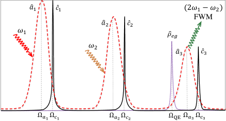
Figure 2: Resonances of the cavity ($\hat{c}_{1,2,3}$, $\Omega_{{c}_{1,2,3}}$) and plasmon ($\hat{a}_{1,2,3}$, $\Omega_{{a}_{1,2,3}}$) modes. Resonance of the QE $\Omega_{\rm\scriptscriptstyle QE}$ is selected around the $\Omega_{a_{3}}$ plasmon mode into which FWM oscillations $\omega_{3}=2\omega_{1}-\omega_{2}$ take place.

The QE is positioned at the hot-spot of the PNS. QE’s resonance, $\Omega_{\rm\scriptscriptstyle QE}$, is chosen such that its coupling (strength $f$) takes place mainly with the FWM plasmon mode ($\Omega_{a_{3}}$), hamiltonian $\hat{\cal H}_{\rm pls\text{-}{\scriptscriptstyle QE}}$. (Choice of the values for $\Omega_{\rm\scriptscriptstyle QE}$ in Figs. 3 and 4 justifies this notion.)

Including also energies of the QE, plasmon and cavity modes, hamiltonian $\hat{\mathcal{H}}_{0}$, the total hamiltonian can be written as

$$\hat{\mathcal{H}}=\hat{\mathcal{H}}_{0}+\hat{\mathcal{H}}_{\text{las-cav}}+\hat{\mathcal{H}}_{\text{cav-pls}}+\hat{\mathcal{H}}_{\rm\scriptscriptstyle FWM}+\hat{\mathcal{H}}_{\text{pls-}{\rm\scriptscriptstyle QE}},$$ (1)

where

$$\hat{\mathcal{H}}_{0}=\hbar\Omega_{\rm\scriptscriptstyle QE}\>\hat{\rho}_{ee}+\hbar\sum_{i=1}^{3}(\Omega_{a_{i}}\hat{a}^{\dagger}_{i}\hat{a}_{i}+\Omega_{c_{i}}\hat{c}^{\dagger}_{i}\hat{c}_{i}),$$ (2)

$$\hat{\mathcal{H}}_{\text{las-cav}}=i\hbar(\hat{c}^{\dagger}_{1}\varepsilon^{(1)}_{L}\text{e}^{-i\omega_{1}t}+\hat{c}^{\dagger}_{2}\varepsilon^{(2)}_{L}\text{e}^{-i\omega_{2}t}-\text{H.c.}),$$ (3)

$$\hat{\mathcal{H}}_{\text{cav-pls}}=\hbar(g_{1}\hat{c}_{1}\hat{a}^{\dagger}_{1}+g_{2}\hat{c}_{2}\hat{a}^{\dagger}_{2}+g_{3}\hat{c}_{3}\hat{a}^{\dagger}_{3}+\text{H.c.}),$$ (4)

$$\hat{\mathcal{H}}_{\rm\scriptscriptstyle FWM}=\hbar\chi_{\rm\scriptscriptstyle FWM}(\hat{a}^{\dagger}_{3}\hat{a}^{\dagger}_{2}\hat{a}^{2}_{1}+\hat{a}^{\dagger 2}_{1}\hat{a}_{2}\hat{a}_{3}),$$ (5)

$$\hat{\cal H}_{\rm pls\text{-}{\scriptscriptstyle QE}}=\hbar(f\hat{a}^{\dagger}_{3}\hat{\rho}_{ge}+f\hat{a}_{3}\hat{\rho}_{eg}).$$ (6)

Here, $\hat{\rho}_{ee}=|e\rangle\langle e|$, $\hat{\rho}_{eg}=|e\rangle\langle g|$ and $\hat{\rho}_{ge}=\hat{\rho}_{eg}^{\dagger}$ represent the density matrices for the QE Scully and Zubairy (1997). $\varepsilon^{(1)}_{L}$ and $\varepsilon^{(2)}_{L}$ are the pump amplitudes/strengths. $\chi_{\rm\scriptscriptstyle FWM}$ is the overlap integral Singh et al. (2016); Tasgın et al. (2018); Ginzburg et al. (2012) for the plasmon modes involving in the FWM process.

Entanglement is originally created among the plasmon modes in the first place. The plasmon modes interact with the cavity modes via a beam-splitter interactions $(\hat{c}_{i}^{\dagger}\hat{a}_{i}+\text{H.c.})$. This transfers the squeezing Ge et al. (2015) into the cavity modes. Moreover, cavity modes are entangled with each other due to entanglement swap mechanism Sen et al. (2005). That is, the entanglement among plasmon modes is swapped into the entanglement among the cavity modes. Cavity modes interact with the cavity output modes $\hat{c}_{\rm out}^{(1\text{-}3)}$ in a similar manner. Thus, the produced multimode entanglement finally swaps into the entanglement among the cavity output modes of three different frequencies.

We mention more about the calculation method of the entanglement in the following paragraphs, but the basics of the mechanism responsible for the entanglement generation is given in the above paragraph. By controlling the QE resonance with an applied voltage, one can control the FWM and the degree of entanglement (link) between different frequencies.

Time-evolution of the modes and QE can be obtained from the Heisenberg equations of motion, e.g., $i\hbar\dot{\hat{a}}=[\hat{a},\hat{H}]$. Including also the damping/decay rates for the cavity fields ($\kappa_{1\text{--}3}=10^{5}$ Hz), plasmon fields ($\gamma_{1\text{--}3}=10^{14}$ Hz) and the QE ($\gamma_{eg}=10^{9}$ Hz), the Langevin equations can be written as

$$\dot{\hat{c}}_{1}= -(\kappa_{1}+i\Omega_{{c}_{1}})\hat{c}_{1}-ig_{1}^{\ast}\hat{a}_{1}+\varepsilon_{L}^{(1)}\text{e}^{-i\omega_{1}t},$$ (7)

$$\dot{\hat{c}}_{2}= -(\kappa_{2}+i\Omega_{{c}_{2}})\hat{c}_{2}-ig_{2}^{\ast}\hat{a}_{2}+\varepsilon_{L}^{(2)}\text{e}^{-i\omega_{2}t},$$ (8)

$$\dot{\hat{c}}_{3}= -(\kappa_{3}+i\Omega_{{c}_{3}})\hat{c}_{3}-ig_{3}^{\ast}\hat{a}_{3},$$ (9)

$$\dot{\hat{a}}_{1}= -(\gamma_{1}+i\Omega_{{a}_{1}})\hat{a}_{1}-ig_{1}\hat{c}_{1}-i2\chi_{\rm\scriptscriptstyle FWM}\hat{a}^{\dagger}_{1}\hat{a}_{2}\hat{a}_{3},$$ (10)

$$\dot{\hat{a}}_{2}= -(\gamma_{2}+i\Omega_{{a}_{2}})\hat{a}_{2}-ig_{2}\hat{c}_{2}-i\chi_{\rm\scriptscriptstyle FWM}\hat{a}_{3}^{\dagger}\hat{a}_{1}^{2},$$ (11)

$$\dot{\hat{a}}_{3}= -(\gamma_{3}+i\Omega_{{a}_{3}})\hat{a}_{3}-ig_{3}\hat{c}_{3}-if\rho_{ge}-i\chi_{\rm\scriptscriptstyle FWM}\hat{a}_{2}^{\dagger}\hat{a}_{1}^{2},$$ (12)

$$\dot{\hat{\rho}}_{ge}= -(\gamma_{eg}+i\Omega_{\rm\scriptscriptstyle QE})\hat{\rho}_{ge}+if\hat{a}_{3}(\hat{\rho}_{gg}-\hat{\rho}_{ee}),$$ (13)

$$\dot{\hat{\rho}}_{ee}= -\gamma_{ee}\hat{\rho}_{ee}+if\hat{a}_{3}^{\dagger}\hat{\rho}_{ge}-if\hat{a}_{3}\hat{\rho}_{eg}.$$ (14)

Here, $\gamma_{ee}$ and $\gamma_{eg}$ are the diagonal and off-diagonal elements decay rates of the QE.

Fano-control of the FWM process.— We calculate the entanglement/squeezing by investigating the noise features (e.g., $\delta\hat{c}$) of the operators around their steady-state values (c-numbers) $\alpha_{c}=\langle\hat{c}\rangle$ with $\hat{c}=\alpha+\delta\hat{c}$. Thus, we first calculate the expectations $\alpha$ for the modes and investigate the fluctuations $\delta\hat{c}$ about them. The calculation of the expectations reveals also the Fano-control (suppression and enhancement) mechanism as follows.

We replace the operators in the Langevin equations (7)-(14) with their expectations. We determine their steady-state values $\alpha_{c_{1}\text{--}c_{3}}$ and $\alpha_{a_{1}\text{--}a_{3}}$, see Sec. 2 of SM sup . For instance, $|\alpha_{a_{3}}|^{2}$ gives the number of generated FWM plasmons at the frequency $\omega_{3}$. As described in Sec. 2 of the SM sup , an analytical expression for the FWM plasmon amplitude can be obtained as

$$\alpha_{a_{3}}=\frac{i\chi_{\rm\scriptscriptstyle FWM}\alpha_{a_{2}}^{\ast}\alpha_{a_{1}}^{2}}{\frac{|f|^{2}y}{i(\Omega_{\rm\scriptscriptstyle QE}-\omega_{3})+\gamma_{eg}}-(i(\Omega_{{a}_{3}}-\omega_{3})+\gamma_{3})},$$ (15)

with $y=\rho_{ee}-\rho_{gg}$ and $\omega_{3}=2\omega_{1}-\omega_{2}$. While we also calculate the numerical values for $\alpha_{a_{3}}$ in Fig. 3, this expression depicts the essential idea below the nonlinearity control. An interference taking place in the denominator of Eq. (15) is in charge for the enhancement of the FWM.

The resonance of the QE $\Omega_{\rm\scriptscriptstyle QE}$ can be arranged (tuned) so that the imaginary part of the first term in the denominator cancels the expression $i(\Omega_{{a}_{3}}-\omega_{3})$ in the second term. This gives the peak in Fig. 3. We note that enhancement factor (EF) given in Fig. 3 multiplies the EFs originating due to the field localization enhancements Singh et al. (2016).

On the contrary, FWM process can be turned off for the choice of $\Omega_{\rm\scriptscriptstyle QE}=\omega_{3}$. In this case, the FWM frequency $\omega_{3}$ production is suppressed. This can be observed from Eq. (15) as follows. $\Omega_{\rm\scriptscriptstyle QE}=\omega_{3}$, the first term of the denominator becomes $|f|^{2}y/\gamma_{eg}$ which turns out to be extremely large because of the small decay rate, e.g., $\gamma_{eg}=10^{-6}\omega_{1}$, of the QE Hallett et al. (2018). We scale frequencies by $\omega_{1}$. The second term of the denominator is below unity and can be neglected besides $|f|^{2}y/\gamma_{eg}$. Thus, the FWM intensity $|\alpha_{a_{3}}|^{2}$ is suppressed by orders of magnitude, see the dip ($10^{-4}$) in Fig. 3.

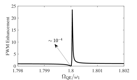
Figure 3: Control of FWM process via the choice of the QE resonance. Plotted enhancement factor (EF) multiplies the EF due to local field enhancement Renger et al. (2009). FWM process can be tuned continuously between $10^{-4}$ ($\Omega_{\rm\scriptscriptstyle QE}=\omega_{3}=1.8000\omega_{1}$) and 25 ($\Omega_{\rm\scriptscriptstyle QE}=\omega_{3}=1.8005\omega_{1}$) via voltage applied on the QE Shibata et al. (2013); Hallett et al. (2018); Chakraborty et al. (2015); Schwarz et al. (2016).

Control of entanglement and squeezing.— The links among different frequency modes can also be controlled by the applied voltage. Entanglement and squeezing features are determined by the quantum fluctuations (quantum noise $\delta\hat{c}_{i}$) about the expectation values $\alpha_{c_{i}}=\langle\hat{c}_{i}\rangle$ Gardiner et al. (2004). We employ a standard method Genes et al. (2008); Vitali et al. (2007) in our calculations. Equations of motions for the noise operators are obtained by inserting, e.g., the expressions $\hat{c}_{i}=\alpha_{i}+\delta\hat{c}_{i}$, into the Langevin equations (7)-(14), and including the noise operators $\delta\hat{c}_{\text{in}}^{(i)}(t)=-i\sum_{k}\text{e}^{-i\omega_{k}^{(i)}t}\>\hat{b}_{k}^{(i)}(0)$, see Sec. 3 of the SM sup . ($\hat{b}_{k}$ are vacuum modes, so $\hat{c}_{\text{in}}^{(i)}$ is the vacuum noise Gardiner et al. (2004).) Ignoring the higher order terms in the equations for the noise operators Genes et al. (2008); Vitali et al. (2007), one obtains

$$\delta\dot{\hat{c}}_{1}= -(\kappa_{1}+i\Delta_{c_{1}})\delta\hat{c}_{1}-ig_{1}^{\ast}\delta\hat{a}_{1}+\delta\hat{c}_{\text{in}}^{(1)}(t),$$ (16)

$$\delta\dot{\hat{c}}_{2}= -(\kappa_{2}+i\Delta_{c_{2}})\delta\hat{c}_{2}-ig_{2}^{\ast}\delta\hat{a}_{2}+\delta\hat{c}_{\text{in}}^{(2)}(t),$$ (17)

$$\delta\dot{\hat{c}}_{3}= -(\kappa_{3}+i\Delta_{c_{3}})\delta\hat{c}_{3}-ig_{3}^{\ast}\delta\hat{a}_{3},$$ (18)

$$\delta\dot{\hat{a}}_{1}= -(\Gamma_{1}+i\Delta_{a_{1}})\delta\hat{a}_{1}-ig_{1}\delta\hat{c}_{1}-i2\chi_{\rm\scriptscriptstyle FWM}$$

$$\times(\alpha_{a_{1}}^{\ast}\alpha_{a_{2}}\delta\hat{a}_{3}+\alpha_{a_{1}}^{\ast}\delta\hat{a}_{2}\alpha_{a_{3}}+\delta\hat{a}_{1}^{\dagger}\alpha_{a_{2}}\alpha_{a_{3}}),$$ (19)

$$\delta\dot{\hat{a}}_{2}= -(\Gamma_{2}+i\Delta_{a_{2}})\delta\hat{a}_{2}-ig_{2}\delta\hat{c}_{2}-i\chi_{\rm\scriptscriptstyle FWM}$$

$$\times(2\alpha_{a_{3}}^{\ast}\alpha_{a_{1}}\delta\hat{a}_{1}+\delta\hat{a}_{3}^{\dagger}\alpha_{a_{1}}^{2}),$$ (20)

$$\delta\dot{\hat{a}}_{3}= -(\Gamma_{3}+i\Delta_{a_{3}})\delta\hat{a}_{3}-ig_{3}\delta\hat{c}_{3}-i\chi_{\rm\scriptscriptstyle FWM}$$

$$\times(2\alpha_{a_{2}}^{\ast}\alpha_{a_{1}}\delta\hat{a}_{1}+\delta\hat{a}_{2}^{\dagger}\alpha_{a_{1}}^{2}).$$ (21)

where $\Delta_{c_{i}}=\omega_{{c}_{i}}-\omega_{i}$ and $\Delta_{a_{i}}=\omega_{{a}_{i}}-\omega_{i}$, with $i=1,2,3$, represent detuning of the cavity and plasmonic modes from the laser fields.

We note that the damping rates $\Gamma_{1\text{--}3}$ we use for the plasmonic noise operators $\delta\hat{a}_{1\text{--}3}$ are different than the ones $\gamma_{1\text{--}3}$ we use in calculating the decay of plasmon excitations. This is due to the following fact. The experiments with PNSs clearly demonstrate Fasel et al. (2005); Tame et al. (2013); Fasel et al. (2006); Huck et al. (2009); Varró et al. (2011); Di Martino et al. (2012) that plasmon excitations can handle nonclassicality features (entanglement and squeezing), determined by the noise operators Simon et al. (1994), for times as long as $10^{-10}$ s. This is only one order lower than, e.g., a quantum dot. We use $\Gamma_{1\text{--}3}=10^{10}$ Hz in our calculation.

We calculate the entanglement among the three output modes of the cavity $\hat{c}_{\text{out}}^{(1\text{--}3)}$ each operating at different frequencies $\omega_{1\text{--}3}$. The output modes are obtained from $\hat{c}_{\text{out}}^{(i)}=r_{i}\hat{c}_{i}(t)+\hat{c}_{\text{in}}^{(i)}$ using the input-output formalism Gardiner et al. (2004); Scully and Zubairy (1997), where $r_{i}$ are constants related with the cavity-vacuum coupling rates. See Sec. 3 of the SM sup .

We use logarithmic negativity (log-neg, $E_{\cal N}$) for quantifying the entanglement Życzkowski et al. (1998); Vidal and Werner (2002); Adesso et al. (2004); Plenio (2005); Tserkis and Ralph (2017). Log-neg is a measure Plenio (2005) of entanglement for Gaussian states. The linearization treatment Genes et al. (2008); Vitali et al. (2007), we employ here, leaves the quantum states Gaussian, so that here we can use log-neg as a measure. We also measure the nonclassicality (e.g., squeezing) of the output modes in units of log-neg. We employ the concept of entanglement-potential Asbóth et al. (2005), which weighs the nonclassicality of a mode in terms of the entanglement it generates after a beams-splitter Asbóth et al. (2005); Tasgin (2020).

In Fig. 4, we present the log-neg entanglement among the three output frequency modes of the cavity, i.e., $\hat{c}_{\text{out}}^{(1)}$-$\hat{c}_{\text{out}}^{(2)}$, $\hat{c}_{\text{out}}^{(2)}$-$\hat{c}_{\text{out}}^{(3)}$, and $\hat{c}_{\text{out}}^{(1)}$-$\hat{c}_{\text{out}}^{(3)}$. Tuning the QE resonance between $\Omega_{\rm\scriptscriptstyle QE}=1.8000\omega_{1}$ and $1.8005\omega_{1}$, one can continuously control the entanglement (link) between different frequencies. The interval $1.8005-1.8000=0.0005\omega_{1}$ corresponds to sub-meV tuning for a typical QE. For instance, in the experiment Shibata et al. (2013) 1 Volt can tune a QD about 10 meV and much betters ones are available Hallett et al. (2018); Chakraborty et al. (2015); Schwarz et al. (2016); Müller et al. (2005); Empedocles and Bawendi (1997).

Figure 4: Entanglement in units of log-neg ($E_{\cal N}$) Życzkowski et al. (1998); Vidal and Werner (2002); Adesso et al. (2004); Plenio (2005) between different frequency output modes of the cavity: $\hat{c}_{\text{out}}^{(1)}$–$\hat{c}_{\text{out}}^{(2)}$ (solid black line), $\hat{c}_{\text{out}}^{(1)}$–$\hat{c}_{\text{out}}^{(3)}$ (red dashed line) and $\hat{c}_{\text{out}}^{(2)}$–$\hat{c}_{\text{out}}^{(3)}$ (dotted green line). Entanglement can be continuously tuned by applied voltage which is below a single volt.

Summary and outlook.— Recent efforts seek programmable and compact QCs capable of generating and executing configurable quantum states and logic gates. An IQC can function at different frequencies. The recent compactness provided by the employment of time-bin encoding Yokoyama et al. (2013); Takeda and Furusawa (2017); Arrazola et al. (2021); Larsen et al. (2021) can be tremendously enhanced by enabling different frequency modes of the IQC to interact with each other Caspani et al. (2016); Kues et al. (2019, 2017); Mahmudlu et al. (2023). Here, we demonstrate the generation of programmable links among different frequency modes, leading to ultra-compact programmable QCs where links can be configured among time-bin encoded photons (modes) functioning at different frequencies. Programmed links among different frequency operations can be established via measurement-induced protocol Filip et al. (2005) without directly coupling the fragile quantum states into nonlinear media. The device operates at sub-picosecond frequencies and is CMOS-compatible. Thus, the device provides a game-changing increase in the capacity, compactness, and controllability of QCs.