Beyond-mean-field theory for the statistics of neuronal coordination

Abstract

Understanding the coordination structure of neurons in neuronal networks is essential for unraveling the distributed information processing mechanisms in brain networks. Recent advancements in measurement techniques have resulted in an increasing amount of data on neural activities recorded in parallel, revealing largely heterogeneous correlation patterns across neurons. Yet, the mechanistic origin of this heterogeneity is largely unknown because existing theoretical approaches linking structure and dynamics in neural circuits are mostly restricted to average connection patterns. Here we present a systematic inclusion of variability in network connectivity via tools from statistical physics of disordered systems. We study networks of spiking leaky integrate-and-fire neurons and employ mean-field and linear-response methods to map the spiking networks to linear rate models with an equivalent neuron-resolved correlation structure. The latter models can be formulated in a field-theoretic language that allows using disorder-average and replica techniques to systematically derive quantitatively matching beyond-mean-field predictions for the mean and variance of cross-covariances as functions of the average and variability of connection patterns. We show that heterogeneity in covariances is not a result of variability in single-neuron firing statistics but stems from the sparse realization and variable strength of connections, as ubiquitously observed in brain networks. Average correlations between neurons are found to be insensitive to the level of heterogeneity, which in contrast modulates the variability of covariances across many orders of magnitude, giving rise to an efficient tuning of the complexity of coordination patterns in neuronal circuits.

I Introduction

Neuronal networks in the brain display largely heterogeneous activity: common observables such as firing rates [1, 2, 3], coefficients of variation (CVs) [4], and pair-wise correlations [5, 6, 7, 8] are widely distributed across neurons. This has important implications for coding and information processing in the brain, as the coordinated activity across the enormous number of units in neuronal circuits is thought to underlie all complex functions [9, 10, 11, 12]. The causes of heterogeneity in neuronal dynamics are diverse: intrinsic neuronal properties, external inputs, and the network connectivity itself are all sources of variability. While these structural and dynamic heterogeneities can be readily observed with modern experimental techniques [13, 14, 15], understanding their mechanistic relations requires theoretical tools that are currently still lacking.

In this study, we focus on the effects of connectivity and investigate the influence of heterogeneity in connections on the activity of networks of identical neurons receiving homogeneous external input. Previous work [16] has shown that a considerable fraction of the variance, in the distribution of firing rates across neurons and in the coefficient of variation (CV) of individual neurons’ spike trains, in such networks can already be explained by the distributed number of inputs the neurons in a network receive. In this study, we go beyond single neuron activities and focus on the statistics of pair-wise correlations and the related covariances, which measure how strongly the activities of pairs of neurons co-fluctuate. Such coordination builds the basis for collective network activity and function.

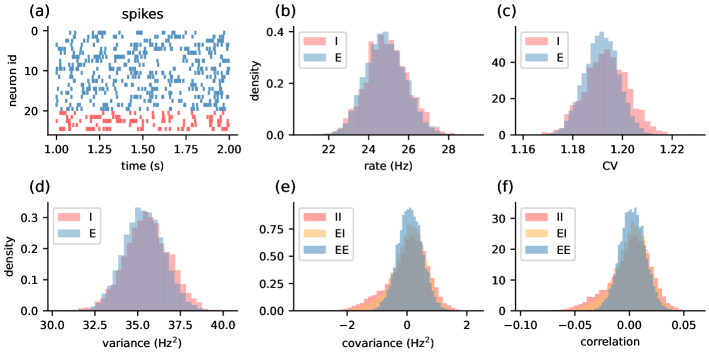
Figure 1: Simulation of excitatory-inhibitory (E-I) network of leaky integrate-and-fire (LIF) neurons. (a) Spike trains of a sample of 20 excitatory (E, blue) and 5 inhibitory (I, red) neurons. (b) Distributions of firing rates. (c) Distributions of coefficients of variation (CVs). (d) Distributions of variances of spike counts measured in time bins of $1\mathrm{s}$ (cf. Eq. (7)). (e) Distributions of spike-count covariances for different pairings of neurons. (f) Distributions of spike-count correlation coefficients for different pairings of neurons. For model details and simulation parameters see Appendix A for spectral radius $r=0.49$.

With the exception of small organisms such as C. elegans [17], the microconnectome of most biological neuronal networks is unknown. However, overall connectivity properties and statistics, like the connection probabilities between different cortical areas [18, 19] and cell types [15], the distance-dependence of connections [20, 15], or the statistics of synaptic strengths [21, 22, 23, 24, 25, 26, 15] are available nowadays. Hence, rather than a one-to-one relation between microconnectome and pair-wise covariances [27, 28, 29, 30, 31, 32], a relation between connectivity and covariance on a statistical level would readily allow the inclusion of this knowledge. To derive such a relation, common population level theories [33, 34, 27, 35, 36, 37, 38] cannot be used because they can only describe population averaged observables and, in particular, do not capture heterogeneity in covariances within populations. Here, we instead employ mean-field theory on the single neuron level [30], which we systematically compare to network simulations, and we go beyond mean-field theory by including non-trivial fluctuation terms to obtain the statistics of covariances between individual neuron pairs.

The main difficulty of a single-neuron level approach is that the predictions of the theory for individual neurons strongly depend on the specific details of the connectivity. To get a description on the level of connectivity statistics, we perform a disorder average, a technique originally developed for spin-glass systems [39, 40] that allows retaining information about the connectivity statistics while averaging over the realization randomness. As our main results, we show how to systematically calculate higher moments of neuronal activity averaged over the disorder in the connectivity using replica and beyond-mean-field theory, and we use this technique to derive a relation between the mean and variance of covariances and the mean and variance of the network connectivity. First results based on a similar but reduced theoretical approach have already been successfully applied in the neuroscientific context to infer the dynamical regime of cortical networks [7] and to explain spatial properties of coordination structures [8] and dimensionality [41].

To summarize, we investigate the origin of neuronal coordination structures, as experimentally observed across various species and cortical areas, by analyzing covariances in a prototypical network model of cortical dynamics [42], namely sparsely connected excitatory and inhibitory neurons that operate in the balanced state [34]. In this model, all neurons have identical parameters and receive homogeneous, uncorrelated external input. As in biological cortical networks, the sparsity in the connectivity between neurons [15], as well as the wide distribution in synaptic amplitudes [21, 22, 23, 24, 25, 26, 15] constitute the source of variability in connections and thereby the dynamics: Rates, CVs, variances, covariances, and hence correlation coefficients are all described by distributions with sizable variance (see Fig. 1).

The following sections investigate the sources of the variance in these quantities. Section II introduces mean-field theory on the single neuron level. In Section III, we derive the main results on how to compute disorder-averaged moments of neuronal activity, and we calculate explicit expressions for the mean and variance of covariances. In Section IV, we discuss our findings and their limitations in the context of the existing literature.

II Background: Linear-response theory of spiking neuronal networks on a single-neuron level

To understand the origin of the distribution of covariances, we start with analyzing a simulated network on a single-neuron level. The network comprises $8000$ excitatory (E) and $2000$ inhibitory (I) leaky integrate-and-fire (LIF) neurons with instantaneous synapses [43, 44] and with random sparse connectivity $\boldsymbol{J}$ (without self connections and prohibiting multiple connections between the same pair of neurons), with $10\,\%$ realized connections (fixed indegree per neuron) and normally distributed synaptic weights $j_{\mathrm{E}}\propto\mathcal{N}\left(j,0.2\cdot j\right)$, $j_{\mathrm{I}}\propto\mathcal{N}\left(gj,0.2\cdot j\right)$, with $g=-6$ (detailed parameters in Appendix A).

Working point

Given the parameters of the simulated network of leaky integrate-and-fire neurons, especially the specific realization of the connectivity matrix $\boldsymbol{J}$, we determine the stationary working point, comprising the input statistics $\left(\boldsymbol{\mu},\boldsymbol{\sigma}\right)$ and the firing rates $\boldsymbol{\nu}$, as done by Brunel and Hakim [45] and Brunel [42]. To this end, we first neglect correlations between the neurons and approximate the neurons’ inputs as independent Gaussian white noise processes. In this diffusion approximation, the mean input $\mu_{i}$ and input variance $\sigma_{i}^{2}$ of neuron $i$ are given by

$$\mu_{i} = \tau_{m}\left(\sum_{j}J_{ij}\nu_{j}+j\nu_{\mathrm{ext},\mathrm{E}}+gj\nu_{\mathrm{ext},\mathrm{I}}+\frac{I_{\mathrm{ext}}}{C}\right)\,,$$ (1)

$$\sigma_{i}^{2} = \tau_{m}\left(\sum_{j}J_{ij}^{2}\nu_{j}+j^{2}\nu_{\mathrm{ext},\mathrm{E}}+g^{2}j^{2}\nu_{\mathrm{ext},\mathrm{I}}\right)\,,$$ (2)

with membrane time constant $\tau_{\mathrm{m}}$, membrane capacitance $C$, constant input current $I_{\mathrm{ext}}$, and excitatory and inhibitory external Poisson noise with rates $\nu_{\mathrm{ext},\mathrm{E}}$ and $\nu_{\mathrm{ext},\mathrm{I}}$ which are fed into the system via weights $j$ and $gj$, respectively. The firing rates are given by the Siegert function [46]

$$\nu_{i} = \left\{\tau_{\mathrm{r}}+\tau_{\mathrm{m}}\sqrt{\pi}\int_{y_{\mathrm{r},i}}^{y_{\mathrm{th},i}}\mathrm{d}s\,f(s)\right\}^{-1}\,,$$ (3)

$$f\left(s\right) = \mathrm{e}^{s^{2}}\left[1+\mathrm{erf}\left(s\right)\right]\,,$$

with refractory period $\tau_{\mathrm{r}}$, and rescaled reset and threshold voltages

$$y_{\mathrm{r},i}=\frac{V_{\mathrm{r}}-\mu_{i}}{\sigma_{i}}\,,\quad y_{\mathrm{th},i}=\frac{V_{\mathrm{th}}-\mu_{i}}{\sigma_{i}}\,.$$

These equations can be solved iteratively in a self-consistent manner. Given the working point, we can determine the coefficients of variation using [42, Appendix A.1, note that they use different units]

$$\mathrm{CV}_{i}^{2}=2\pi\left(\tau_{\mathrm{m}}\nu_{i}\right)^{2}\int_{y_{\mathrm{r},i}}^{y_{\mathrm{th},i}}\mathrm{d}x\>\mathrm{e}^{x^{2}}\int_{-\infty}^{x}\mathrm{d}z\,\mathrm{e}^{z^{2}}\left[1+\mathrm{erf}\left(z\right)\right]^{2}\,.$$ (4)

Linearization

The full dynamics of LIF neurons are non-linear. However, as covariances measure co-fluctuations of neurons around their working points, we can study covariances by analyzing linearized dynamics as long as the fluctuations are sufficiently small. Grytskyy et al. [31, Section 5] show that a network of LIF neurons can be mapped to a linear rate model with output noise

$$x_{i}\left(t\right)=\int_{-\infty}^{t}h(t-t^{\prime})\sum_{j}W_{ij}\left[x_{j}\left(t^{\prime}-d\right)+\xi_{j}\left(t^{\prime}-d\right)\right]\,dt^{\prime},$$ (5)

with neuronal activity $x_{i}\left(t\right)$, normalized linear response kernel $h(t)$, synaptic delay $d$, and uncorrelated Gaussian white noise $\xi_{i}\left(t\right)$, $\left\langle\xi_{i}\right\rangle=0$, $\left\langle\xi_{i}\left(s\right)\xi_{j}\left(t\right)\right\rangle=D_{ij}\delta\left(s-t\right)$, with diagonal noise strength matrix $D_{ij}=\delta_{ij}D_{ii}$. The matrix $\boldsymbol{W}$, referred to as effective connectivity, combines the connectivity matrix $\boldsymbol{J}$ with the sensitivity of neurons to small fluctuations in their input. It is formally given by the derivative of the stationary firing rate of neuron $i$ Eq. (3) with respect to the firing rate of neuron $j$ evaluated at the stationary working point [47, Appendix A]

$$W_{ij}=\frac{\partial\nu_{i}}{\partial\nu_{j}}=\alpha_{i}J_{ij}+\beta_{i}J_{ij}^{2}\,,$$ (6)

with

$$\alpha_{i} = \sqrt{\pi}\left(\tau_{\mathrm{m}}\nu_{i}\right)^{2}\frac{1}{\sigma_{i}}\left[f\left(y_{\mathrm{th},i}\right)-f\left(y_{\mathrm{r},i}\right)\right]\,,$$

$$\beta_{i} = \sqrt{\pi}\left(\tau_{\mathrm{m}}\nu_{i}\right)^{2}\frac{1}{2\sigma_{i}^{2}}\left[f\left(y_{\mathrm{th},i}\right)y_{\mathrm{th},i}-f\left(y_{\mathrm{r},i}\right)y_{\mathrm{r},i}\right]\,.$$

Spike-count covariances

In this study we are interested in spike-count covariances in spiking networks

$$C_{ij}=\frac{1}{T}\left(\left\langle n_{i}n_{j}\right\rangle-\left\langle n_{i}\right\rangle\left\langle n_{j}\right\rangle\right)\,,$$ (7)

with spike counts $n_{i}$ occurring within bins of size $T$, where the average is taken across all bins. As shown in Dahmen et al. [7, Materials and Methods], for stationary processes and large bin sizes spike-count covariances $C_{ij}$ can be mapped to the time-lag integrated covariances $c_{ij}(\tau)$ between spike trains of neurons $i$ and $j$ (48, 49, see also, for more details on definitions of covariances see Appendix B)

$$C_{ij}\overset{T\rightarrow\infty}{\rightarrow}\int_{-\infty}^{\infty}c_{ij}\left(\tau\right)d\tau\,.$$

In the following the term covariance always refers to $C_{ij}$. Making use of the Wiener-Khinchin theorem (C) allows expressing the time-lag integrated covariances in terms of the neuronal activities’ Fourier components $X_{i}\left(\omega\right)$ at frequency zero

$$C_{ij}=\left\langle X_{i}\left(0\right)X_{j}\left(0\right)\right\rangle\,,$$ (8)

which can be evaluated by Fourier transforming Eq. (5), yielding

$$\boldsymbol{C}=\left(\boldsymbol{1}-\boldsymbol{W}\right)^{-1}\boldsymbol{D}\left(\boldsymbol{1}-\boldsymbol{W}\right)^{-\mathrm{T}}\,.$$ (9)

For calculating the covariances, we therefore only need the effective connectivity $\boldsymbol{W}$ and the noise strength $\boldsymbol{D}$. The correlation coefficients follow as

$$\kappa_{ij}=\frac{C_{ij}}{\sqrt{C_{ii}C_{jj}}}\,.$$

To estimate the noise strength $\boldsymbol{D}$, we assume that the spike trains are described sufficiently well as renewal processes for which the variances are given by [50]

$$C_{ii}=CV_{i}^{2}\nu_{i}\,.$$ (10)

Using that $\boldsymbol{D}$ is diagonal, we can solve Eq. (9) for $\boldsymbol{D}$, which results in

$$D_{ii}=\sum_{j}\left(B^{-1}\right)_{ij}CV_{j}^{2}\nu_{j}\,,$$ (11)

with

$$B_{ij}=\left[\left(\boldsymbol{1}-\boldsymbol{W}\right)^{-1}\right]_{ij}^{2}\,.$$ (12)

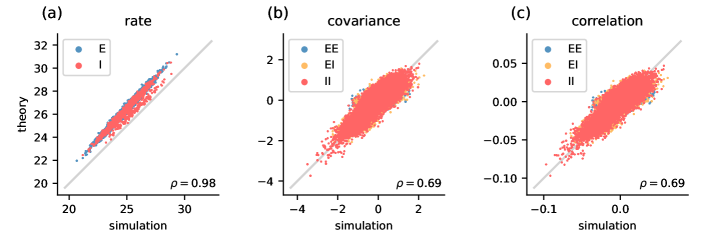
Figure 2: Simulation results and theoretical estimates for E-I network of LIF neurons. Here $\rho$ denotes the Pearson correlation coefficient. (a) Firing rates $\boldsymbol{\nu}$. (b) Covariances $\boldsymbol{C}$. (c) Correlation coefficients $\boldsymbol{\kappa}$. For model details and simulation parameters see A for spectral radius $r=0.49$.

The above expressions can be combined to compute theoretical estimates of the quantities measured in the simulation. To solve the self-consistency equations for the firing rates and to compute the covariances, we make use of the python package NNMT [51], which includes optimized implementations of the equations introduced above. A comparison of theoretical and simulation results is shown in Fig. 2. For the chosen parameters, simulation and theory correlate strongly, and the theory appears to capture the primary sources of heterogeneity in the rates, covariances, and correlation coefficients. Note that such a good match between theory and simulation can not be observed in all parameter regimes of the spiking network; the validity of the assumptions made and the resulting theoretical estimates depend on the network state (see Appendix D for further discussion on valid parameter regimes). Fig. 2 also reveals some unexplained variance, particularly pronounced in the covariances and correlations. This variance is the result of the finite simulation time and the associated uncertainty in the estimated covariances. As we show in Appendix K, the covariance estimate bias can be significant and it can only be corrected for on a statistical level rather than for individual covariances. Focusing on the statistics of covariances, however, has further advantages: For realistic network sizes, Eq. (9) is a high-dimensional equation that depends on each and every connection in the network. Understanding general mechanisms relating network structure and dynamics is therefore difficult. The covariance statistics instead summarize the most important aspects of covariances and, for large neuron populations, can be assumed to be self-averaging [52, 53, 40], which makes them less dependent on connectivity details. Second, Eq. (9) cannot be used for inference based on experimentally measured parameters because as of yet it is neither possible to determine the effective connectivity nor covariances of all neurons in a network. And lastly, as stated above, we will demonstrate that covariance statistics are more robust measures than single-neuron covariances, both with respect to finite measurements as well as to the assumptions made in the derivation above.

III Statistical description of covariances

The expression (9) reveals that the statistics of the covariances $\boldsymbol{C}$, in particular their heterogeneity, is determined by the statistics and heterogeneity of the effective connectivity matrix $\boldsymbol{W}$ and the external noise strength $\boldsymbol{D}$. Our aim here is to derive a description of the cross-covariance statistics in terms of the statistics of $\boldsymbol{W}$ and $\boldsymbol{D}$. To this end, we derive analytical expressions for the mean and the variance of the time-lag integrated cross-covariances averaged over the heterogeneities of the system.

To do this, simply averaging Eq. (9) is not feasible due to $\boldsymbol{W}$ appearing in the inverse matrix $\left(\boldsymbol{1}-\boldsymbol{W}\right)^{-1}$. Performing an average over a random connectivity is, however, a well known problem in the theory of disordered systems [52, 54, 55, 40], where it is handled on the level of generating functions. To proceed analogously, we start with Eq. (8), which expresses the covariances in terms of the moments of the dynamic variables’ Fourier components at frequency zero. This allows us to write the covariances in terms of the moment-generating function $Z\left(\boldsymbol{J}\right)$ of the zero-frequency Fourier components $X_{i}$ of the dynamical equation (5) (see Appendix E for more details):

$$C_{ij}=\left\langle X_{i}X_{j}\right\rangle=\left.\frac{\mathrm{\partial}}{\partial J_{i}}\frac{\mathrm{\partial}}{\partial J_{j}}Z\left(\boldsymbol{J}\right)\right|_{\boldsymbol{J}=0}\,,$$

with

$$Z\left(\boldsymbol{J}\right) = \frac{\widetilde{Z}\left(\boldsymbol{J}\right)}{\widetilde{Z}\left(\boldsymbol{0}\right)}$$

$$= \left|\det\left(1-\boldsymbol{W}\right)\right|\int\mathcal{D}\boldsymbol{X}\int\mathcal{D}\widetilde{\boldsymbol{X}}$$

$$\times\exp\left[\widetilde{\boldsymbol{X}}^{\mathrm{T}}\left(\boldsymbol{1}-\boldsymbol{W}\right)\boldsymbol{X}+\frac{1}{2}\widetilde{\boldsymbol{X}}^{\mathrm{T}}\boldsymbol{D}\widetilde{\boldsymbol{X}}+\boldsymbol{J}^{\mathrm{T}}\boldsymbol{X}\right]\,,$$

and $\widetilde{Z}\left(\boldsymbol{0}\right)^{-1}=\left|\det\left(1-\boldsymbol{W}\right)\right|$. Here, $\widetilde{\boldsymbol{X}}$ are auxiliary variables that can be used to calculate the response function $\left\langle X_{i}\widetilde{X}_{j}\right\rangle$ of neuron $i$ to a perturbation of neuron $j$ by introducing additional sources $\widetilde{\boldsymbol{J}}$ in the moment-generating function (see Appendix E). Equation (III) shows that calculating the disorder-average of the covariances boils down to calculating the disorder-average of the moment-generating function. In the following two sections, we use this approach to calculate the mean of the cross-covariances $\left\langle\boldsymbol{C}\right\rangle_{\boldsymbol{W},\boldsymbol{D}}$ and subsequently the variance of the cross-covariances $\left\langle\delta\boldsymbol{C}^{2}\right\rangle_{\boldsymbol{W},\boldsymbol{D}}$.

III.1 Mean of cross-covariances

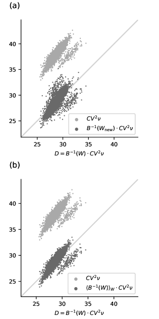
Figure 3: Effect of averaging noise strength over disorder in $\boldsymbol{W}$ and effect of applying $\boldsymbol{B}^{-1}$ on variances. (a) Noise strength computed using the procedure described above (noise strength in the following) vs. noise strength computed using a new realization of $\boldsymbol{W}$ (dark gray), and noise strength vs. variances (light gray). (b) Noise strength vs. noise strength computed using an average over $100$ realizations of $\boldsymbol{W}$ (dark gray) and noise strength vs. variances (light gray). Spectral radius $r=0.49$.

Disorder average

We begin with the mean cross-covariances, focusing first on the average over the ensemble of connectivities. In the moment generating function Eq. (III), $\boldsymbol{W}$ occurs linearly in the exponent of $\widetilde{Z}\left(\boldsymbol{J}\right)$, which is advantageous for performing the disorder-average. However, the averaging procedure is complicated by two aspects: 1) $\boldsymbol{W}$ contributes to the noise strength $\boldsymbol{D}$ through the variance-rescaling matrix $\boldsymbol{B}^{-1}$, and 2) the normalization $\widetilde{Z}\left(\boldsymbol{0}\right)$ depends on $\boldsymbol{W}$. However, as illustrated in Fig. 3, in practice the first point does not appear to be a problem: Panel a indicates that the specifics of $\boldsymbol{D}$ are largely determined by the details of the variances $\boldsymbol{CV}^{2}\boldsymbol{\nu}$, because a different realization of $\boldsymbol{W}$ essentially yields a similar $\boldsymbol{D}$, and Panel b suggests that the effect of the disorder-average on $\boldsymbol{D}$ is minimal. For these reasons, we treat $\boldsymbol{D}$ as though it was independent of the explicit realization of $\boldsymbol{W}$. To address the second point, an alternative approach based on the moment-generating functional for the full time-dependent dynamics (see Appendix E) could be utilized. This moment-generating functional has a unit determinant normalization independent of $\boldsymbol{W}$ [56]. The disorder-average of its frequency space complement, however, introduces cross-frequency couplings that complicate the further analysis. Here, instead, we follow Dahmen et al. [7], and separate the averages over $\widetilde{Z}\left(\boldsymbol{J}\right)$ and $\widetilde{Z}\left(\boldsymbol{0}\right)$

$$\left\langle Z\left(\boldsymbol{J}\right)\right\rangle_{\boldsymbol{W}} =\left\langle\frac{\widetilde{Z}\left(\boldsymbol{J}\right)}{\widetilde{Z}\left(\boldsymbol{0}\right)}\right\rangle_{\boldsymbol{W}}\approx \frac{\left\langle\widetilde{Z}\left(\boldsymbol{J}\right)\right\rangle_{\boldsymbol{W}}}{\left\langle\widetilde{Z}\left(\boldsymbol{0}\right)\right\rangle_{\boldsymbol{W}}}\,,$$ (14)

as we find that this factorization approach does yield accurate results. This leaves us with the task of calculating $\left\langle\widetilde{Z}\left(\boldsymbol{J}\right)\right\rangle_{\boldsymbol{W}}$.

The disorder-average only affects the coupling term and can be expressed using the moment-generating functions $\phi_{ij}$ of $W_{ij}$

$$\left\langle\exp\left(-\widetilde{\boldsymbol{X}}^{\mathrm{T}}\boldsymbol{W}\boldsymbol{X}\right)\right\rangle_{\boldsymbol{W}} =\left\langle\prod_{i,j}\exp\left(-W_{ij}\widetilde{X}_{i}X_{j}\right)\right\rangle_{\boldsymbol{W}}$$

$$=\prod_{i,j}\phi_{ij}\left(-\widetilde{X}_{i}X_{j}\right)\,,$$

assuming independently drawn weights $W_{ij}\sim p_{ij}\left(W_{ij}\right)$. The moment-generating function can be written in terms of a cumulant expansion $\phi_{ij}\left(X\right)=\exp\left(\sum_{k=1}^{\infty}\kappa_{k,ij}X^{k}/k!\right)$, with $k$-th cumulants $\kappa_{k,ij}\,$. For fixed connection probability, the number of inputs to a neuron scales with the network size $N$. To keep the input and its fluctuations finite when increasing the network size, we require synaptic weights to scale with $1/\sqrt{N}$ [34, 57], such that the cumulant expansion is an expansion in $1/\sqrt{N}$. A truncation at the second cumulant ($\propto N^{-1}$) maps $\boldsymbol{W}$ to a Gaussian connectivity with distribution $\mathcal{N}\left(\boldsymbol{M},\boldsymbol{\Delta}/N\right)$, such that

$$\left\langle\widetilde{Z}\left(\boldsymbol{J}\right)\right\rangle_{W} = \int\mathcal{D}\boldsymbol{X}\int\mathcal{D}\widetilde{\boldsymbol{X}}$$ (16)

$$\times\exp\left[S_{0}\left(\boldsymbol{X},\widetilde{\boldsymbol{X}}\right)+\boldsymbol{J}^{\mathrm{T}}\boldsymbol{X}\right]$$

$$\times\exp\left[\frac{1}{2N}\sum_{i,j}\Delta_{ij}\widetilde{X}_{i}\widetilde{X}_{i}X_{j}X_{j}\right]\,,$$

with

$$S_{0}\left(\boldsymbol{X},\widetilde{\boldsymbol{X}}\right)=\widetilde{\boldsymbol{X}}^{\mathrm{T}}\left(\boldsymbol{1}-\boldsymbol{M}\right)\boldsymbol{X}+\frac{1}{2}\widetilde{\boldsymbol{X}}^{\mathrm{T}}\boldsymbol{D}\widetilde{\boldsymbol{X}}\,,$$

and mean connection weights $M_{ij}=\mathcal{O}\left(1/\sqrt{N}\right)$ as well as variances $\Delta_{ij}=\mathcal{O}(1)$.

Auxiliary field formulation

To deal with the four-point coupling term in Eq. (16), we define auxiliary variables $Q_{i}:=\frac{1}{N}\sum_{j}\Delta_{ij}X_{j}X_{j}$, which we formally introduce by inserting an identity in the form of a Fourier transformed delta distribution

$$1 = \prod_{i}\int\mathrm{d}Q_{i}\,\delta\left(\frac{1}{N}\sum_{j}\Delta_{ij}X_{j}X_{j}-Q_{i}\right)$$

$$= \prod_{i}N\int_{-\infty}^{\infty}\mathrm{d}Q_{i}\int_{-\mathrm{i}\infty}^{\mathrm{i}\infty}\frac{\mathrm{d}\widetilde{Q}_{i}}{2\pi\mathrm{i}}\,$$

$$\times\exp\left[\widetilde{Q}_{i}\left(\sum_{j}\Delta_{ij}X_{j}X_{j}-NQ_{i}\right)\right]\,.$$

The auxiliary variables $\widetilde{Q}_{i}$ have been introduced to express the delta distribution as an integral. This leads to

$$\left\langle\widetilde{Z}\left(\boldsymbol{J}\right)\right\rangle_{\boldsymbol{W}} = \int\mathcal{D}\boldsymbol{Q}\int\mathcal{D}\widetilde{\boldsymbol{Q}}\,\exp\left(-N\boldsymbol{Q}^{T}\widetilde{\boldsymbol{Q}}\right)$$

$$\times \underbrace{\int\mathcal{D}\boldsymbol{X}\int\mathcal{D}\widetilde{\boldsymbol{X}}\,\exp\left[S_{\boldsymbol{Q},\widetilde{\boldsymbol{Q}}}\left(\boldsymbol{X},\widetilde{\boldsymbol{X}}\right)+\boldsymbol{J}^{\mathrm{T}}\boldsymbol{X}\right]}_{=:\widetilde{Z}_{\boldsymbol{Q},\widetilde{\boldsymbol{Q}}}\left(\boldsymbol{J}\right)}\,,$$

$$S_{\boldsymbol{Q},\widetilde{\boldsymbol{Q}}}\left(\boldsymbol{X},\widetilde{\boldsymbol{X}}\right) = \widetilde{\boldsymbol{X}}^{\mathrm{T}}\left(\boldsymbol{1}-\boldsymbol{M}\right)\boldsymbol{X}$$ (18)

$$+ \frac{1}{2}\widetilde{\boldsymbol{X}}^{\mathrm{T}}\left[\boldsymbol{D}+\mathrm{diag}\left(\boldsymbol{Q}\right)\right]\widetilde{\boldsymbol{X}}$$

$$+ \boldsymbol{X}^{\mathrm{T}}\mathrm{diag}\left(\widetilde{\boldsymbol{Q}}^{\mathrm{T}}\boldsymbol{\Delta}\right)\boldsymbol{X}\,.$$

Here $\mathrm{diag}\left(\boldsymbol{Q}\right)_{ij}$ refers to a diagonal matrix with diagonal elements $Q_{i}$. As the action $S_{\boldsymbol{Q},\widetilde{\boldsymbol{Q}}}\left(\boldsymbol{X},\widetilde{\boldsymbol{X}}\right)$ at fixed auxiliary variables describes an auxiliary free theory, Eq. (III.1) describes the activity of linear rate neurons in a network with disorder-averaged connectivity $\boldsymbol{M}$ that interact with fluctuating external variables $\boldsymbol{Q}$ and $\widetilde{\boldsymbol{Q}}$. Inserting Eq. (III.1) into Eq. (14) yields

$$\left\langle Z\left(\boldsymbol{J}\right)\right\rangle_{\boldsymbol{W}} = \int\mathcal{D}\boldsymbol{Q}\int\mathcal{D}\widetilde{\boldsymbol{Q}}\,\frac{\widetilde{Z}_{\boldsymbol{Q},\widetilde{\boldsymbol{Q}}}\left(\boldsymbol{J}\right)}{\widetilde{Z}_{\boldsymbol{Q},\widetilde{\boldsymbol{Q}}}\left(\boldsymbol{0}\right)}$$

$$\times\frac{\exp\left(-N\boldsymbol{Q}^{T}\widetilde{\boldsymbol{Q}}\right)\widetilde{Z}_{\boldsymbol{Q},\widetilde{\boldsymbol{Q}}}\left(\boldsymbol{0}\right)}{\int\mathcal{D}\boldsymbol{P}\int\mathcal{D}\widetilde{\boldsymbol{P}}\,\exp\left(-N\boldsymbol{P}^{T}\widetilde{\boldsymbol{P}}\right)\widetilde{Z}_{\boldsymbol{P},\widetilde{\boldsymbol{P}}}\left(\boldsymbol{0}\right)}$$

$$=: \int\mathcal{D}\boldsymbol{Q}\int\mathcal{D}\widetilde{\boldsymbol{Q}}\,p\left(\boldsymbol{Q},\widetilde{\boldsymbol{Q}}\right)Z_{\boldsymbol{Q},\widetilde{\boldsymbol{Q}}}\left(\boldsymbol{J}\right)\,,$$

with joint probability distribution

$$p\left(\boldsymbol{Q},\widetilde{\boldsymbol{Q}}\right) = \frac{\exp\left(-S\left(\boldsymbol{Q},\widetilde{\boldsymbol{Q}}\right)\right)}{\int\mathcal{D}\boldsymbol{P}\int\mathcal{D}\widetilde{\boldsymbol{P}}\,\exp\left(-S\left(\boldsymbol{P},\widetilde{\boldsymbol{P}}\right)\right)}\,,$$

$$S\left(\boldsymbol{Q},\widetilde{\boldsymbol{Q}}\right) = N\boldsymbol{Q}^{T}\widetilde{\boldsymbol{Q}}-\ln\left[\widetilde{Z}_{\boldsymbol{Q},\widetilde{\boldsymbol{Q}}}\left(\boldsymbol{0}\right)\right]\,,$$ (19)

and properly normalized moment generating function $Z_{\boldsymbol{Q},\widetilde{\boldsymbol{Q}}}\left(\boldsymbol{J}\right)=\widetilde{Z}_{\boldsymbol{Q},\widetilde{\boldsymbol{Q}}}\left(\boldsymbol{J}\right)/\widetilde{Z}_{\boldsymbol{Q},\widetilde{\boldsymbol{Q}}}\left(\boldsymbol{0}\right)$. These equations imply that the disorder-average of arbitrary moments $\left\langle X_{i_{1}}\dots X_{i_{k}}\right\rangle$ can be calculated by determining the corresponding moments $\left\langle X_{i_{1}}\dots X_{i_{k}}\right\rangle_{\boldsymbol{Q},\widetilde{\boldsymbol{Q}}}$ with respect to the auxiliary free theory and averaging them over the auxiliary variables

$$\left\langle\left\langle X_{i_{1}}\dots X_{i_{k}}\right\rangle\right\rangle_{\boldsymbol{W}} = \int\mathcal{D}\boldsymbol{Q}\int\mathcal{D}\widetilde{\boldsymbol{Q}}\,$$

$$\times p\left(\boldsymbol{Q},\tilde{\boldsymbol{Q}}\right)\left\langle X_{i_{1}}\dots X_{i_{k}}\right\rangle_{\boldsymbol{Q},\widetilde{\boldsymbol{Q}}}\,,$$

$$\left\langle X_{i_{1}}\dots X_{i_{k}}\right\rangle_{\boldsymbol{Q},\widetilde{\boldsymbol{Q}}} = \left.\frac{\partial}{\partial J_{i_{1}}}\dots\frac{\partial}{\partial J_{i_{k}}}Z_{\boldsymbol{Q},\widetilde{\boldsymbol{Q}}}\left(\boldsymbol{J}\right)\right|_{\boldsymbol{J}=\boldsymbol{0}}\,.$$

Saddle-point approximation

Due to the prefactor $N$ in Eq. (19) and the scalar products in $\widetilde{Z}_{\boldsymbol{Q},\widetilde{\boldsymbol{Q}}}\left(\boldsymbol{0}\right)$ with $N$ contributions, we expect $p\left(\boldsymbol{Q},\widetilde{\boldsymbol{Q}}\right)$ to peak sharply for $N\rightarrow\infty$, such that we can perform a saddle-point approximation. To lowest order, we expect $p\left(\boldsymbol{Q},\widetilde{\boldsymbol{Q}}\right)\approx\delta\left(\boldsymbol{Q}-\boldsymbol{Q}^{*}\right)\delta\left(\widetilde{\boldsymbol{Q}}-\widetilde{\boldsymbol{Q}}^{*}\right)$, with the saddle-point $\boldsymbol{Q}^{*},\widetilde{\boldsymbol{Q}}^{*}$ determined by

$$\left.\frac{\partial}{\partial\widetilde{Q}_{i}}S\left(\boldsymbol{Q},\widetilde{\boldsymbol{Q}}\right)\right|_{\boldsymbol{Q}^{*},\widetilde{\boldsymbol{Q}}^{*}}=0\,,\quad\left.\frac{\partial}{\partial Q_{i}}S\left(\boldsymbol{Q},\widetilde{\boldsymbol{Q}}\right)\right|_{\boldsymbol{Q}^{*},\widetilde{\boldsymbol{Q}}^{*}}=0\,,$$

which yields

$$Q_{i}^{*} = \frac{1}{N}\sum_{j}\Delta_{ij}\left\langle X_{j}X_{j}\right\rangle_{\boldsymbol{Q}^{*},\widetilde{\boldsymbol{Q}}^{*}}\,,$$ (21)

$$\widetilde{Q}_{i}^{*} = \frac{1}{2N}\left\langle\widetilde{X}_{i}\widetilde{X}_{i}\right\rangle_{\boldsymbol{Q}^{*},\widetilde{\boldsymbol{Q}}^{*}}\,,$$

with second moments evaluated at the saddle-point. The moments can be calculated explicitly by solving the Gaussian integrals (see Appendix F). Using the shorthand $\boldsymbol{R}\coloneqq\left(\boldsymbol{1}-\boldsymbol{M}\right)^{-1}$, we find $\left\langle X_{i}X_{j}\right\rangle_{\boldsymbol{Q}^{*},\widetilde{\boldsymbol{Q}}^{*}}=\left\{\boldsymbol{R}\left[\boldsymbol{D}+\mathrm{diag}\left(\boldsymbol{Q}^{*}\right)\right]\boldsymbol{R}^{\mathrm{T}}\right\}_{ij}$ and $\left\langle\widetilde{X}_{i}\widetilde{X}_{i}\right\rangle_{\boldsymbol{Q}^{*},\widetilde{\boldsymbol{Q}}^{*}}=0$, and solving for the saddle point yields

$$Q_{i}^{*} = \frac{1}{N}\sum_{j,k,l,m}\left(\boldsymbol{1}-\frac{1}{N}\Delta\cdot\left(\boldsymbol{R}\odot\boldsymbol{R}\right)\right)_{ij}^{-1}\Delta_{jk}R_{kl}D_{lm}R_{km}\,,$$

$$\widetilde{Q}_{i}^{*} = 0\,,$$

with $\odot$ denoting the element-wise (Hadamard) product.

Finally, making use of the Wiener-Khinchin theorem Eq. (38) and inserting the solution of the saddle-point equations into Eq. (III.1) yields the mean covariances averaged across the disorder of the connectivity

$$\left\langle\boldsymbol{C}\right\rangle_{\boldsymbol{W}} =\left\langle\boldsymbol{X}\boldsymbol{X}^{\mathrm{T}}\right\rangle_{\boldsymbol{Q}^{*},\widetilde{\boldsymbol{Q}}^{*}}$$

$$=\left(\boldsymbol{1}-\boldsymbol{M}\right)^{-1}\left[\boldsymbol{D}+\mathrm{diag}\left(\boldsymbol{Q}^{*}\right)\right]\left(\boldsymbol{1}-\boldsymbol{M}\right)^{-\mathrm{T}}\,.$$

Averaging over the disorder in $\boldsymbol{D}$ then yields

$$\left\langle\boldsymbol{C}\right\rangle_{\boldsymbol{W},\boldsymbol{D}}$$ (22)

$$=(\boldsymbol{1} -\boldsymbol{M})^{-1}\left\{\overline{\boldsymbol{D}}+\mathrm{diag}\left[\boldsymbol{Q}^{*}\left(\boldsymbol{D}=\overline{\boldsymbol{D}}\right)\right]\right\}\left(\boldsymbol{1}-\boldsymbol{M}\right)^{-\mathrm{T}}\,.$$

Here $\overline{\boldsymbol{D}}$ denotes the disorder-averaged noise strength (cf. Fig. 3b and discussion after Eq. (III.2)). Note that the saddle point $\boldsymbol{Q}^{*}\left(\boldsymbol{D}=\overline{\boldsymbol{D}}\right)$ together with $\overline{\boldsymbol{D}}$ yields an effective noise strength which shifts average variances and covariances. Importantly, it is only the heterogeneity in the connectivity $\boldsymbol{W}$ that causes this shift. Average covariances are insensitive to heterogeneity in the noise strengths $\boldsymbol{D}$; they only depend on the average $\overline{\boldsymbol{D}}$.

III.2 Variance of cross-covariances

Replica method

Calculating the variances of covariances across the ensemble of possible network connectivities

$$\left\langle\delta\boldsymbol{C}^{2}\right\rangle_{\boldsymbol{W}} = \left\langle\boldsymbol{C}\odot\boldsymbol{C}\right\rangle_{\boldsymbol{W}}-\left\langle\boldsymbol{C}\right\rangle_{\boldsymbol{W}}\odot\left\langle\boldsymbol{C}\right\rangle_{\boldsymbol{W}}$$ (23)

requires making use of the replica method [58, 40] and deriving an expression for the disorder-averaged moment-generating function of the replicated system $\left\langle Z\left(\boldsymbol{J}\right)Z\left(\boldsymbol{K}\right)\right\rangle_{\boldsymbol{W}}$, as this allows calculating disorder averages of arbitrary squared moments $\left\langle\left\langle X_{i_{1}}\dots X_{i_{k}}\right\rangle^{2}\right\rangle_{\boldsymbol{W}}$, which occur in the first term in Eq. (23). The procedure is completely analogous to the previous section’s derivations. However, the disorder-average now affects the term

$$\left\langle\exp\left(\widetilde{\boldsymbol{X}}^{\mathrm{T}}\boldsymbol{W}\boldsymbol{X}+\widetilde{\boldsymbol{Y}}^{\mathrm{T}}\boldsymbol{W}\boldsymbol{Y}\right)\right\rangle_{\boldsymbol{W}}$$

$$=\prod_{i,j}\exp\Bigg{[}\sum_{k=1}^{\infty}\frac{\kappa_{k,ij}}{k!} \left(\widetilde{X}_{i}X_{j}+\widetilde{Y}_{i}Y_{j}\right){}^{k}\Bigg{]}\,,$$

where $\boldsymbol{X}$ and $\boldsymbol{Y}$ refer to the activity in the first and second replicon, respectively. A cumulant expansion up to second order introduces — along four-point couplings separately in $\boldsymbol{X}$ and $\boldsymbol{Y}$ similar to the one in Eq. (16) — a replica coupling term

$$\exp\left(\frac{1}{N}\sum_{ij}\Delta_{ij}\widetilde{X}_{i}\widetilde{Y}_{i}X_{j}Y_{j}\right)\,.$$

To deal with the four-point couplings, we again introduce auxiliary variables

$$Q_{XX,i} = \frac{1}{N}\sum_{j}\Delta_{ij}X_{j}X_{j}\,,$$

$$Q_{YY,i} = \frac{1}{N}\sum_{j}\Delta_{ij}Y_{j}Y_{j}\,,$$

$$Q_{XY,i} = \frac{1}{N}\sum_{j}\Delta_{ij}X_{j}Y_{j}\,,$$

and obtain a relation similar to Eq. (III.1),

$$\left\langle\left\langle X_{i_{1}}\dots X_{i_{k}}\right\rangle^{2}\right\rangle_{\boldsymbol{W}} =\int\mathcal{D}\boldsymbol{Q}\int\mathcal{D}\widetilde{\boldsymbol{Q}}\,$$ (24)

$$\times p\left(\boldsymbol{Q},\widetilde{\boldsymbol{Q}}\right) \left\langle X_{i_{1}}\dots X_{i_{k}}Y_{i_{1}}\dots Y_{i_{k}}\right\rangle_{\boldsymbol{Q},\widetilde{\boldsymbol{Q}}}\,,$$

$$\left\langle X_{i_{1}}\dots X_{i_{k}}Y_{i_{1}}\dots Y_{i_{k}}\right\rangle_{\boldsymbol{Q},\widetilde{\boldsymbol{Q}}}$$

$$=\frac{\partial}{\partial J_{i_{1}}}\dots\frac{\partial}{\partial J_{i_{k}}} \frac{\partial}{\partial K_{i_{1}}}\dots\left.\frac{\partial}{\partial K_{i_{k}}}Z_{\boldsymbol{Q},\widetilde{\boldsymbol{Q}}}\left(\boldsymbol{J},\boldsymbol{K}\right)\right|_{\boldsymbol{J},\boldsymbol{K}=\boldsymbol{0}}\,,$$

but with

$$p\left(\boldsymbol{Q},\widetilde{\boldsymbol{Q}}\right) =\frac{\exp\left(-S\left(\boldsymbol{Q},\widetilde{\boldsymbol{Q}}\right)\right)}{\int\mathcal{D}\boldsymbol{P}\int\mathcal{D}\widetilde{\boldsymbol{P}}\,\exp\left(-S\left(\boldsymbol{P},\widetilde{\boldsymbol{P}}\right)\right)}\,,$$

$$\mathcal{S}\left(\boldsymbol{Q},\widetilde{\boldsymbol{Q}}\right) =N\boldsymbol{Q}_{XX}^{\mathrm{T}}\widetilde{\boldsymbol{Q}}_{XX}+N\boldsymbol{Q}_{XY}^{\mathrm{T}}\widetilde{\boldsymbol{Q}}_{XY}$$ (25)

$$+N\boldsymbol{Q}_{YY}^{\mathrm{T}}\widetilde{\boldsymbol{Q}}_{YY}-\ln\widetilde{Z}_{\boldsymbol{Q},\widetilde{\boldsymbol{Q}}}\left(\boldsymbol{0},\boldsymbol{0}\right)\,,$$

$$\widetilde{Z}_{\boldsymbol{Q},\widetilde{\boldsymbol{Q}}}\left(\boldsymbol{J},\boldsymbol{K}\right) =\int\mathcal{D}\boldsymbol{X}\int\mathcal{D}\widetilde{\boldsymbol{X}}\int\mathcal{D}\boldsymbol{Y}\int\mathcal{D}\widetilde{\boldsymbol{Y}}$$

$$\times\exp \Big{[}S_{\boldsymbol{Q}_{XX},\widetilde{\boldsymbol{Q}}_{XX}}\left(\boldsymbol{X},\widetilde{\boldsymbol{X}}\right)+S_{\boldsymbol{Q}_{YY},\widetilde{\boldsymbol{Q}}_{YY}}\left(\boldsymbol{Y},\widetilde{\boldsymbol{Y}}\right)$$

$$+\widetilde{\boldsymbol{X}}^{\mathrm{T}}\mathrm{diag}\left(\boldsymbol{Q}_{XY}\right)\widetilde{\boldsymbol{Y}}+\boldsymbol{X}^{\mathrm{T}}\mathrm{diag}\left(\widetilde{\boldsymbol{Q}}_{XY}^{\mathrm{T}}\boldsymbol{\Delta}\right)\boldsymbol{Y}$$

$$+\boldsymbol{J}^{\mathrm{T}}\boldsymbol{X}+\boldsymbol{K}^{\mathrm{T}}\boldsymbol{Y}\Big{]}\,,$$

$$Z_{\boldsymbol{Q},\widetilde{\boldsymbol{Q}}}\left(\boldsymbol{J},\boldsymbol{K}\right) =\widetilde{Z}_{\boldsymbol{Q},\widetilde{\boldsymbol{Q}}}\left(\boldsymbol{J},\boldsymbol{K}\right)/\widetilde{Z}_{\boldsymbol{Q},\widetilde{\boldsymbol{Q}}}\left(\boldsymbol{0},\boldsymbol{0}\right)\,,$$

where $\boldsymbol{Q}$ and $\widetilde{\boldsymbol{Q}}$ are shorthand notations denoting all auxiliary variables, and $S_{\boldsymbol{Q}_{XX},\widetilde{\boldsymbol{Q}}_{XX}}\left(\boldsymbol{X},\widetilde{\boldsymbol{X}}\right)$ and $S_{\boldsymbol{Q}_{YY},\widetilde{\boldsymbol{Q}}_{YY}}\left(\boldsymbol{Y},\widetilde{\boldsymbol{Y}}\right)$ are given by Eq. (18).

Saddle-point approximation

As in Section III.1, we approximate $p\left(\boldsymbol{Q},\widetilde{\boldsymbol{Q}}\right)$ as a delta function at the saddle-point $\boldsymbol{Q}^{*},\widetilde{\boldsymbol{Q}}^{*}$ (for details see Appendix F), and with Eq. (24) to lowest order we get

$$\left\langle C_{ij}^{2}\right\rangle_{\boldsymbol{W}} = \left\langle\left\langle X_{i}X_{j}\right\rangle^{2}\right\rangle_{\boldsymbol{W}}$$

$$= \int\mathcal{D}\boldsymbol{Q}\int\mathcal{D}\widetilde{\boldsymbol{Q}}\,p\left(\boldsymbol{Q},\widetilde{\boldsymbol{Q}}\right)\left\langle X_{i}X_{j}Y_{i}Y_{j}\right\rangle_{\boldsymbol{Q},\widetilde{\boldsymbol{Q}}}$$

$$= \int\mathcal{D}\boldsymbol{Q}\int\mathcal{D}\widetilde{\boldsymbol{Q}}\,p\left(\boldsymbol{Q},\widetilde{\boldsymbol{Q}}\right)$$

$$\times\Big{(}\left\langle X_{i}X_{j}\right\rangle_{\boldsymbol{Q},\widetilde{\boldsymbol{Q}}}\left\langle Y_{i}Y_{j}\right\rangle_{\boldsymbol{Q},\widetilde{\boldsymbol{Q}}}$$

$$+\left\langle X_{i}Y_{i}\right\rangle_{\boldsymbol{Q},\widetilde{\boldsymbol{Q}}}\left\langle X_{j}Y_{j}\right\rangle_{\boldsymbol{Q},\widetilde{\boldsymbol{Q}}}$$

$$+\left\langle X_{i}Y_{j}\right\rangle_{\boldsymbol{Q},\widetilde{\boldsymbol{Q}}}\left\langle X_{j}Y_{i}\right\rangle_{\boldsymbol{Q},\widetilde{\boldsymbol{Q}}}\Big{)}$$

$$\approx \left\langle X_{i}X_{j}\right\rangle_{\boldsymbol{Q}^{*},\widetilde{\boldsymbol{Q}}^{*}}\left\langle Y_{i}Y_{j}\right\rangle_{\boldsymbol{Q}^{*},\widetilde{\boldsymbol{Q}}^{*}}$$

$$+\left\langle X_{i}Y_{i}\right\rangle_{\boldsymbol{Q}^{*},\widetilde{\boldsymbol{Q}}^{*}}\left\langle X_{j}Y_{j}\right\rangle_{\boldsymbol{Q}^{*},\widetilde{\boldsymbol{Q}}^{*}}$$

$$+\left\langle X_{i}Y_{j}\right\rangle_{\boldsymbol{Q}^{*},\widetilde{\boldsymbol{Q}}^{*}}\left\langle X_{j}Y_{i}\right\rangle_{\boldsymbol{Q}^{*},\widetilde{\boldsymbol{Q}}^{*}}$$

$$= \left\langle X_{i}X_{j}\right\rangle_{\boldsymbol{Q}^{*},\widetilde{\boldsymbol{Q}}^{*}}\left\langle Y_{i}Y_{j}\right\rangle_{\boldsymbol{Q}^{*},\widetilde{\boldsymbol{Q}}^{*}}$$

$$\approx \left\langle\left\langle X_{i}X_{j}\right\rangle\right\rangle_{\boldsymbol{W}}^{2}$$

$$= \left\langle C_{ij}\right\rangle_{\boldsymbol{W}}^{2}\,,$$ (27)

where we used Wick’s theorem, which is allowed by the fact that, for $\boldsymbol{Q}$ and $\widetilde{\boldsymbol{Q}}$ given and fixed, $\widetilde{Z}_{\boldsymbol{Q},\widetilde{\boldsymbol{Q}}}\left(\boldsymbol{J},\boldsymbol{K}\right)$ describes a Gaussian theory, and the fact that all cross-replica correlators $\left\langle X_{i}Y_{j}\right\rangle_{\boldsymbol{Q}^{*},\widetilde{\boldsymbol{Q}}^{*}}$ vanish at the saddle point (see Appendix F).

Fluctuations around the saddle-point

Eq. (27) implies that the variance of covariances is zero in the saddle-point approximation, and we need to account for Gaussian fluctuations of the auxiliary fields around their saddle-points by making a Gaussian approximation of $p\left(\boldsymbol{Q},\widetilde{\boldsymbol{Q}}\right)$. The crucial fluctuations are the ones of $\boldsymbol{Q}_{XY}$ and $\widetilde{\boldsymbol{Q}}_{XY}$, as they can potentially preserve the replica coupling and thus lead to non-vanishing variance contributions of cross-replica correlators $\left\langle X_{i}Y_{i}\right\rangle_{\boldsymbol{Q}^{*},\widetilde{\boldsymbol{Q}}^{*}}$. Away from the saddle-points, the correlators in Eq. (III.2) depend on $\boldsymbol{Q}$ and $\widetilde{\boldsymbol{Q}}$ in a complicated manner. To render the integrals in Eq. (III.2) solvable in the Gaussian approximation, we perform a Taylor expansion of the correlators around the saddle points $\boldsymbol{Q}^{*},\widetilde{\boldsymbol{Q}}^{*}$, which effectively is an expansion of $\widetilde{Z}_{\boldsymbol{Q},\widetilde{\boldsymbol{Q}}}\left(\boldsymbol{J},\boldsymbol{K}\right)$ (see Appendix G for more details). In the first term of Eq. (III.2), leading order fluctuations in $\boldsymbol{Q}_{XY}$ and $\widetilde{\boldsymbol{Q}}_{XY}$ depend on correlators with an odd number of variables of each replicon. Therefore, this term cannot yield a contribution to the variance due to fluctuations of $\boldsymbol{Q}_{XY}$ and $\widetilde{\boldsymbol{Q}}_{XY}$. The major replica coupling arises from the second and third term in Eq. (III.2). We note that the third term contains off-diagonal elements of correlators which are suppressed by a factor $1/N$ with respect to the diagonal ones. Therefore, we can neglect this term for cross-covariances as well and only keep the second term in Eq. (III.2) as the leading order contribution. For autocovariances the second and third term in Eq. (III.2) are the same, yielding an additional factor $2$. Introducing $\delta\boldsymbol{Q}=\boldsymbol{Q}-\boldsymbol{Q}^{*}$ and defining $\delta\widetilde{\boldsymbol{Q}}$ equivalently, we obtain

$$\left\langle X_{i}Y_{i}\right\rangle_{\boldsymbol{Q},\widetilde{\boldsymbol{Q}}} =\sum_{k}\left\langle X_{i}Y_{i}\widetilde{X}_{k}\widetilde{Y}_{k}\right\rangle_{\boldsymbol{Q}^{*},\widetilde{\boldsymbol{Q}}^{*}}\delta Q_{XY,k}$$

$$+\sum_{k,l} \Delta_{kl}\left\langle X_{i}Y_{i}X_{l}Y_{l}\right\rangle_{\boldsymbol{Q}^{*},\widetilde{\boldsymbol{Q}}^{*}}\delta\widetilde{Q}_{XY,k}+\mathcal{O}\left(\left|\delta\boldsymbol{Q}\right|^{2},\left|\delta\widetilde{\boldsymbol{Q}}\right|^{2}\right)$$

$$=\sum_{k}\left\langle X_{i}\widetilde{X}_{k}\right\rangle_{\boldsymbol{Q}^{*},\widetilde{\boldsymbol{Q}}^{*}}^{2}\delta Q_{XY,k}$$

$$+\sum_{k,l} \Delta_{kl}\left\langle X_{i}X_{l}\right\rangle_{\boldsymbol{Q}^{*},\widetilde{\boldsymbol{Q}}^{*}}^{2}\delta\widetilde{Q}_{XY,k}+\mathcal{O}\left(\left|\delta\boldsymbol{Q}\right|^{2},\left|\delta\widetilde{\boldsymbol{Q}}\right|^{2}\right)\,,$$ (28)

where we used that cross-replica correlators vanish at the saddle point. Inserting the above fluctuation expansion result around $\boldsymbol{Q}_{XY}^{*}$ and $\widetilde{\boldsymbol{Q}}_{XY}^{*}$ into Eq. (III.2) leads to

$$\int \mathcal{D}\boldsymbol{Q}\int\mathcal{D}\widetilde{\boldsymbol{Q}}\,p\left(\boldsymbol{Q},\widetilde{\boldsymbol{Q}}\right)\left\langle X_{i}Y_{i}\right\rangle_{\boldsymbol{Q},\widetilde{\boldsymbol{Q}}}\left\langle X_{j}Y_{j}\right\rangle_{\boldsymbol{Q},\widetilde{\boldsymbol{Q}}}$$

$$=\sum_{k,l}\left\langle X_{i}\widetilde{X}_{k}\right\rangle_{\boldsymbol{Q}^{*},\widetilde{\boldsymbol{Q}}^{*}}^{2}\left\langle X_{j}\widetilde{X}_{l}\right\rangle_{\boldsymbol{Q}^{*},\widetilde{\boldsymbol{Q}}^{*}}^{2}\left\langle\delta Q_{XY,k}\delta Q_{XY,l}\right\rangle_{\boldsymbol{Q},\widetilde{\boldsymbol{Q}}}$$

$$+\sum_{k,l,m}\left\langle X_{i}\widetilde{X}_{k}\right\rangle_{\boldsymbol{Q}^{*},\widetilde{\boldsymbol{Q}}^{*}}^{2}\Delta_{lm}\left\langle X_{j}X_{m}\right\rangle_{\boldsymbol{Q}^{*},\widetilde{\boldsymbol{Q}}^{*}}^{2}\left\langle\delta Q_{XY,k}\delta\widetilde{Q}_{XY,l}\right\rangle_{\boldsymbol{Q},\widetilde{\boldsymbol{Q}}}$$

$$+\sum_{k,l,m}\left\langle X_{j}\widetilde{X}_{k}\right\rangle_{\boldsymbol{Q}^{*},\widetilde{\boldsymbol{Q}}^{*}}^{2}\Delta_{lm}\left\langle X_{i}X_{m}\right\rangle_{\boldsymbol{Q}^{*},\widetilde{\boldsymbol{Q}}^{*}}^{2}\left\langle\delta Q_{XY,k}\delta\widetilde{Q}_{XY,l}\right\rangle_{\boldsymbol{Q},\widetilde{\boldsymbol{Q}}}$$

$$+\sum_{k,l,m,n}\left\langle X_{i}X_{m}\right\rangle_{\boldsymbol{Q}^{*},\widetilde{\boldsymbol{Q}}^{*}}^{2}\left\langle X_{j}X_{n}\right\rangle_{\boldsymbol{Q}^{*},\widetilde{\boldsymbol{Q}}^{*}}^{2}\Delta_{km}\Delta_{ln}$$

$$\quad\times\left\langle\delta\widetilde{Q}_{XY,k}\delta\widetilde{Q}_{XY,l}\right\rangle_{\boldsymbol{Q},\widetilde{\boldsymbol{Q}}}\,.$$ (29)

Next, we consider the Gaussian approximation of $p\left(\boldsymbol{Q},\widetilde{\boldsymbol{Q}}\right)$ with

$$\mathcal{S}\left(\boldsymbol{Q},\widetilde{\boldsymbol{Q}}\right)=\mathcal{S}\left(\boldsymbol{Q}^{*},\widetilde{\boldsymbol{Q}}^{*}\right)+\frac{1}{2}\left(\delta\boldsymbol{Q}_{XY},\delta\widetilde{\boldsymbol{Q}}_{XY}\right)\boldsymbol{\mathcal{S}}^{(2)}\left(\begin{array}[]{c}\delta\boldsymbol{Q}_{XY}\\ \delta\widetilde{\boldsymbol{Q}}_{XY}\end{array}\right)\,,$$

where $\boldsymbol{S}^{(2)}$ contains the second derivatives with respect to the auxiliary fields

$$\boldsymbol{S}^{(2)}=\left(\begin{array}[]{cc}\left.\frac{\partial\mathcal{S}\left(\boldsymbol{Q},\widetilde{\boldsymbol{Q}}\right)}{\partial\boldsymbol{Q}_{XY}\partial\boldsymbol{Q}_{XY}}\right|_{\boldsymbol{Q}^{*},\widetilde{\boldsymbol{Q}}^{*}}&\left.\frac{\partial\mathcal{S}\left(\boldsymbol{Q},\widetilde{\boldsymbol{Q}}\right)}{\partial\boldsymbol{Q}_{XY}\partial\widetilde{\boldsymbol{Q}}_{XY}}\right|_{\boldsymbol{Q}^{*},\widetilde{\boldsymbol{Q}}^{*}}\\ \left.\frac{\partial\mathcal{S}\left(\boldsymbol{Q},\widetilde{\boldsymbol{Q}}\right)}{\partial\widetilde{\boldsymbol{Q}}_{XY}\partial\boldsymbol{Q}_{XY}}\right|_{\boldsymbol{Q}^{*},\widetilde{\boldsymbol{Q}}^{*}}&\left.\frac{\partial\mathcal{S}\left(\boldsymbol{Q},\widetilde{\boldsymbol{Q}}\right)}{\partial\widetilde{\boldsymbol{Q}}_{XY}\partial\widetilde{\boldsymbol{Q}}_{XY}}\right|_{\boldsymbol{Q}^{*},\widetilde{\boldsymbol{Q}}^{*}}\end{array}\right)\,,$$

which allows evaluating the correlators of the auxiliary fields in Eq. (29) (see Appendix H for details). Inserting the results, to leading order we find (see Appendix I for details)

$$\left\langle C_{ij}^{2}\right\rangle_{\boldsymbol{W}} = \left(1+\delta_{ij}\right)\biggl{[}\left(\boldsymbol{1}-\frac{1}{N}\boldsymbol{R}^{\mathrm{T}}\odot\boldsymbol{R}^{\mathrm{T}}\boldsymbol{\Delta}\right)^{-1}\left\langle\boldsymbol{X}\boldsymbol{X}^{\mathrm{T}}\right\rangle_{\boldsymbol{Q}^{*},\widetilde{\boldsymbol{Q}}^{*}}$$ (30)

$$\odot\left\langle\boldsymbol{X}\boldsymbol{X}^{\mathrm{T}}\right\rangle_{\boldsymbol{Q}^{*},\widetilde{\boldsymbol{Q}}^{*}}\left(\boldsymbol{1}-\frac{1}{N}\boldsymbol{R}^{\mathrm{T}}\odot\boldsymbol{R}^{\mathrm{T}}\boldsymbol{\Delta}\right)^{-\mathrm{T}}\biggr{]}_{ij}$$

$$-\delta_{ij}\left\langle C_{ij}\right\rangle_{\boldsymbol{W}}^{2}\,.$$

To get the variances rather than the second moments, we subtract the squared mean covariances $\left\langle C_{ij}\right\rangle_{\boldsymbol{W}}^{2}$. However, for the setup that we study here the squared mean cross-covariances are of the order $\mathcal{O}\left(1/N^{2}\right)$ and therefore negligible. Taking into account that $\boldsymbol{R}=\left(\boldsymbol{1}-\boldsymbol{M}\right)^{-1}\approx\boldsymbol{1}$, which holds as long as the network is inhibition dominated, we find the following expression for the disorder-averaged variance of cross-covariances (see Appendix I for full expression)

$$\left\langle\delta\boldsymbol{C}^{2}\right\rangle_{\boldsymbol{W}} = \left(\boldsymbol{1}-\boldsymbol{S}\right)^{-1}\left\{\boldsymbol{D}+\mathrm{diag}\left[\boldsymbol{Q}^{*}\left(\boldsymbol{D}\right)\right]\right\}$$

$$\odot\left\{\boldsymbol{D}+\mathrm{diag}\left[\boldsymbol{Q}^{*}\left(\boldsymbol{D}\right)\right]\right\}\left(\boldsymbol{1}-\boldsymbol{S}\right)^{-\mathrm{T}}\,,$$

where we wrote $\boldsymbol{S=}\boldsymbol{\Delta}/N$.

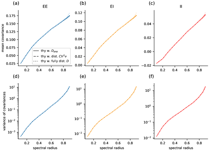
Figure A5: Dependence of population-resolved covariance statistics (Fig. A5 and Eq. (III.2) ) on heterogeneity in noise strength $\boldsymbol{D}$. The continuous lines show the results using the realization independent estimate of $\boldsymbol{D}$ Eq. (32). For the dashed lines, Eq. (32) with the single-neuron resolved estimates of $CV_{i}^{2}\nu_{i}$ introduced in Section II was used, whereas the dotted lines show the results using the full single-neuron resolved estimate of $\boldsymbol{D}$ (Eq. (11)). (a, b, c) Mean cross-covariances. (d, e, f) Variance of cross-covariances.

However, if the noise strength $\boldsymbol{D}$ has to be estimated using Eq. (11), this expression is still dependent on the specific realization of $\boldsymbol{W}$, both implicitly through the estimates of the single-neuron rates and CVs described in Section II and explicitly through the matrix $\boldsymbol{B}$ (Eq. (12)). Since the right hand side of Eq. (III.2) depends non-linearly on $\boldsymbol{D}$, averaging over the statistics of $\boldsymbol{D}$ introduces terms depending on the heterogeneity of $\boldsymbol{D}$. However, Fig. A5 in the Appendix shows that heterogeneity in $\boldsymbol{D}$ — both via the explicit dependence on $\boldsymbol{W}$ and via the implicit dependence through distributed firing rates and CVs — is negligible for the statistics of cross-covariances. This can be understood by considering the structure of Eq. (III.2): The matrices $\left(\boldsymbol{1}-\boldsymbol{S}\right)^{-1}$ are multiplied with $\boldsymbol{D}$, such that any heterogeneity in $\boldsymbol{D}$ is averaged out. An E-I network is an illustrative example, with $\left(\boldsymbol{1}-\boldsymbol{S}\right)^{-1}=\boldsymbol{1}+\boldsymbol{U}$ with a $2\times 2$ block matrix $\boldsymbol{U}$ whose entries are homogeneous in each population block, such that the matrix product effectively is an average over $\boldsymbol{D}$.

To obtain an average $\boldsymbol{D}$ that is not depending on a specific realization of $\boldsymbol{W}$, we follow Eq. (11) and set

$$\overline{D}_{ii}=\sum_{j}\left(\boldsymbol{1}-\boldsymbol{S}\right)_{ij}\cdot\overline{CV_{j}^{2}}\overline{\nu_{j}}\,,$$ (32)

which inserted into the disorder-averaged expression for the autocovariances (Eq. (22)) yields the correct autocovariances:

$$C_{ii} =\left[\left(\boldsymbol{1}-\boldsymbol{M}\right)^{-1}\left\{\overline{\boldsymbol{D}}+\mathrm{diag}\left[\boldsymbol{Q}^{*}\left(\overline{\boldsymbol{D}}\right)\right]\right\}\left(\boldsymbol{1}-\boldsymbol{M}\right)^{-\mathrm{T}}\right]_{ii}$$

$$\approx\left\{\overline{\boldsymbol{D}}+\mathrm{diag}\left[\left(\boldsymbol{1}-\boldsymbol{S}\right)^{-1}\boldsymbol{S}\cdot\mathrm{diag}\left(\overline{\boldsymbol{D}}\right)\right]\right\}_{ii}$$

$$=\sum_{j}\left(\boldsymbol{1}-\boldsymbol{S}\right)_{ij}^{-1}\overline{D}_{jj}$$

$$=\overline{CV_{i}^{2}}\overline{\nu_{i}}\,.$$

Here we used $\left(\boldsymbol{1}-\boldsymbol{M}\right)^{-1}\approx\boldsymbol{1}$ and $\boldsymbol{Q}^{*}\approx\left(\boldsymbol{1}-\boldsymbol{S}\right)^{-1}\boldsymbol{S}\cdot\mathrm{diag}\left(\boldsymbol{D}\right)$. The realization-independent estimates $\overline{\nu_{i}}$ and $\overline{CV_{i}^{2}}$ of the rates and CVs, respectively, can be obtained using standard population-resolved mean-field theory [45, 42], which only requires knowing the statistics of $\boldsymbol{W}$. A procedure similar to the one described in Section II can be used: In the population view, however, the indices $i,j$ no longer denote single neurons but rather populations of equal neurons. In Eq. (1) $J_{ij}$ is replaced by $K_{ij}J_{ij}$ and $J_{ij}^{2}$ in Eq. (2) is replaced by $K_{ij}J_{ij}^{2}$, where $K_{ij}$ is the indegree from population $j$ to population $i$, and $J_{ij}$ then is interpreted as the mean synaptic weight from population $j$ to population $i$.

Replacing $\boldsymbol{D}$ in Eq. (III.2) by Eq. (32) yields a fully realization-independent disorder-averaged estimate of the variance of cross-covariances.

III.3 Singularities

Next, we discuss the interpretation of the derived formulae. Thereto, we need to have a closer look at the effective noise strength $\boldsymbol{D}+\mathrm{diag}\left[\boldsymbol{Q}^{*}\left(\boldsymbol{D}\right)\right]$, which occurs in both the mean (Eq. (22)) and the variances (Eq. (III.2)) of covariances. Using Eq. (32), we find that the impact of heterogeneity on the effective noise cancels:

$$\mathrm{diag}\left(\boldsymbol{D}\right)+\boldsymbol{Q}^{*}\left(\boldsymbol{D}\right) \approx\mathrm{diag}\left(\boldsymbol{D}\right)+\left(\boldsymbol{1}-\boldsymbol{S}\right)^{-1}\boldsymbol{S}\cdot\mathrm{diag}\left(\boldsymbol{D}\right)$$

$$=\left(\boldsymbol{1}-\boldsymbol{S}\right)^{-1}\cdot\mathrm{diag}\left(\boldsymbol{D}\right)$$ (33)

$$=\left(\boldsymbol{1}-\boldsymbol{S}\right)^{-1}\left(\boldsymbol{1}-\boldsymbol{S}\right)\cdot\boldsymbol{a}$$

$$\approx\boldsymbol{a}\>,$$

where $a_{i}=\overline{CV_{i}^{2}}\overline{\nu_{i}}$ is the vector of estimated autocovariances. This is because we specifically chose the noise strength $\boldsymbol{D}$ such that autocovariances match those from the spiking networks: As heterogeneity is increased, external fluctuations get amplified by the factor $\left(\boldsymbol{1}-\boldsymbol{S}\right)^{-1}$ in Eq. (33). To achieve that autocovariances do not diverge, external inputs need to be scaled down according to Eq. (32). Hence, the mean and variance of cross-covariances are given by

$$\left\langle\boldsymbol{C}\right\rangle_{\boldsymbol{W},\boldsymbol{D}} \approx\left(\boldsymbol{1}-\boldsymbol{M}\right)^{-1}\mathrm{diag}\left(\boldsymbol{a}\right)\left(\boldsymbol{1}-\boldsymbol{M}\right)^{-\mathrm{T}}$$ (34)

$$\left\langle\delta\boldsymbol{C}^{2}\right\rangle_{\boldsymbol{W,D}} \approx\left(\boldsymbol{1}-\boldsymbol{S}\right)^{-1}\mathrm{diag}\left(\boldsymbol{a}\right)\odot\mathrm{diag}\left(\boldsymbol{a}\right)\left(\boldsymbol{1}-\boldsymbol{S}\right)^{-\mathrm{T}}\,.$$ (35)

Note that any inverse matrix can be written as $\boldsymbol{A}^{-1}=\det\left(\boldsymbol{A}\right)^{-1}\mathrm{adj}\left(\boldsymbol{A}\right)$, where $\mathrm{adj}\left(\boldsymbol{A}\right)$ denotes the adjugate matrix. As a result, the elements of an inverse matrix $\boldsymbol{A}^{-1}$ diverge if the determinant of the matrix $\boldsymbol{A}$ vanishes, which occurs when at least one eigenvalue of $\boldsymbol{A}$ is zero. Therefore, the divergence behavior of the mean and variance of covariances is determined by the eigenvalues of $\boldsymbol{M}$ and $\boldsymbol{S}$ with real parts close to $1$.

Eq. (34) reveals that mean cross-covariances are determined by the mean connectivity $\boldsymbol{M}$. By choosing $\boldsymbol{D}$ to match the autocovariances of the spiking model, they are, in particular, unaffected by network heterogeneity, represented by $\boldsymbol{S}$. A range of important network properties, such as population structure determining E-I balance [34, 36, 37, 47, 59], spatial structure like distance-dependent connection probabilities [60, 61, 62, 63, 64, 65, 8], or low-rank structures [66], can be encoded in $\boldsymbol{M}$. Divergences in mean covariances, caused by eigenvalues of $\boldsymbol{M}$ close to $1$, can thus be indicative of phenomena like loss of E-I balance with excessive excitation (cf. 59, Fig. 8D) or instability of the homogeneously active state in spatially organized networks [67].

Variances of cross-covariances are determined by network heterogeneity (Eq. (35)), encoded in the connectivity variance $\boldsymbol{S}$ and are to leading order independent of the mean connectivity $\boldsymbol{M}$. Note that sub-leading terms nevertheless can become sizable if eigenvalues of $\boldsymbol{M}$ are close to the instability line at $1$. As demonstrated by Aljadeff et al. [68], if $\boldsymbol{S}$ is a block structured matrix, its eigenvalue spectrum is circular, with a spectral radius $r$ that is determined by the square root of the maximum eigenvalue of $\boldsymbol{S}$. For the simple E-I network with target-agnostic connectivity studied here, the spectral radius is given by [69]

$$r^{2}=N_{\mathrm{E}}\sigma_{\mathrm{E}}^{2}+N_{\mathrm{I}}\sigma_{\mathrm{I}}^{2}\,.$$

The spectral radius, a measure of network heterogeneity, increases when the variance of synaptic strength grows, which is controlled by an interplay between the connection probabilities of different populations and the variances of the associated synaptic weights. Intuitively, as explained in Dahmen et al. [8], multi-synaptic signal transmission is very efficient in a network with a large spectral radius, such that pairs of neurons influence each other via a large number of neuronal pathways, possibly including differing numbers of excitatory and inhibitory neurons. The effects of these various pathways add up, and the large variety of potential pathways results in a broad distribution of covariances.

We see that the effects of $\boldsymbol{M}$ and $\boldsymbol{S}$ are mostly independent of one another, allowing the mean and variance of covariances to vary separately. This, however, only applies to synaptic weights that are identically and independently distributed (i.i.d.). If the weights are correlated, such as through chain structures in the connectivity, the respective eigenvalues cannot be changed independently. A more detailed analysis of this behavior is to be published elsewhere. As a final remark, it is worth noting that the independence of the mean covariances of $\boldsymbol{S}$ confirms that previously employed population models [36, 37, 47, 31, 59], which neglect the variance of connectivity, are valid for computing mean covariances.

To illustrate how the mean and variance of covariances change as functions of the network heterogeneity, we plot Eq. (22) and Eq. (III.2) with Eq. (32) for spectral radii between $0$ and $1$ in Fig. 4 (predicted linear). We kept the working point roughly constant for the different spectral radii by maintaining the mean $\mu$ and variance $\sigma^{2}$ of the total input to each neuron while modifying the synaptic efficacy. To compensate for the increased intrinsic input and fluctuations at larger spectral radii, we reduced the mean and fluctuations of the external input.

Confirming the discussion of Eq. (34) and Eq. (35), when the spectral radius is modified, the variances of covariances vary by several orders of magnitude, whereas mean covariances remain in the same order of magnitude. A range of prior research [37, 31, 59] has shown that a divergence of mean covariances would be observed as a function of E-I balance, e.g. by altering $g$. Here we focus on network scenarios away from the excitatory instability (fixed $g=-6$) and therefore do not see a divergence of mean covariances. Nevertheless, we observe a change of mean covariances when changing the spectral radius. This is because in the sparse random network chosen here, the variance of the synaptic weights is not independent from the mean of the weights. Adjusting the spectral radius requires modifying the weights, resulting in the residual change in the mean covariances visible in Fig. 4a, b, and c. Note that by keeping the working point of the network constant across spectral radii, we also keep the noise strength factor in Eq. (22) and Eq. (III.2) constant (cf. Eq. (34) and Eq. (35)). If the external noise strength was instead determined by a fixed external process, i.e $\boldsymbol{D}$ independent of $\boldsymbol{W}$, then mean covariances would also diverge as a function of the spectral radius due to the factor $\left(\boldsymbol{1}-\boldsymbol{S}\right)^{-1}$, which enters the noise strength term via $\boldsymbol{Q}^{*}$.

III.4 Comparison of prediction and measurement of covariance statistics

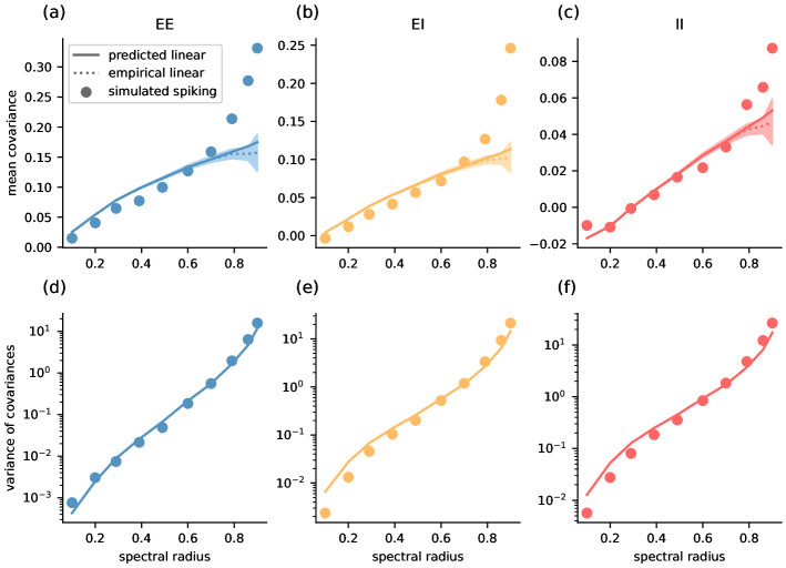
Figure 4: Covariance statistics for EE, EI, and II connections at different spectral radii. Dots show the population resolved mean (Panels a, b, c) or variance (Panels d, e, f) of the spike count cross-covariances (Eq. (7)) measured in spiking network simulations. Solid lines show the theoretical predictions of the mean (Eq. (22)) and variance (Eq. (III.2)) of cross-covariances, respectively, using the noise strength estimate Eq. (32). The dashed lines show the population resolved empirical mean and variance of cross-covariances from Eq. (9) averaged over 20 realizations of $W$, and the shaded area depicts a two standard deviation range around the mean. The variances computed from the simulation results have been corrected for bias due to finite simulation time (see Appendix K).

To check how closely the predictions match the outcomes of spiking network simulations, we ran 10 simulations for different spectral radii similarly to the one shown in Fig. 1 using the parameters specified in A. We ensured that the spiking networks have roughly similar working points for the different spectral radii in the same way we calculated the theoretical values (see Appendix Fig. A2a, b). We computed the mean and variance of the measured covariances and corrected the variances for bias due to finite simulation time (see Appendix K for details). The results are displayed in Fig. 4.

We observe that the order of magnitude of mean and variance are well predicted by Eq. (22) and Eq. (III.2), which is especially evident for the variances (Panels d,e,f), which span several orders of magnitude. However, there is some quantitative discrepancy between the predictions of the presented linear theory and the results of the simulated spiking network, which is visible in Panels a, b, and c, indicating that a linear theory cannot fully capture the non-linear spiking dynamics at high spectral radii, where potential non-renewal effects of spiking arise [70]. To verify that the discrepancy originates mostly from the linear-response approximation rather than our disorder-average approximations, we plotted the predictions of the linear theory Eq. (9) for 20 different network realizations: At small spectral radii, the predicted disorder-average based mean is equal to the empirical mean of the linear networks, and for large spectral radii, the predicted mean appears to be within the range of two standard deviations around the empirical mean. This shows that the deviations to the spiking network results mostly stem from the linear-response approximation. The remaining difference between the predicted and the empirical mean in linear networks could be explained by the fact that for high spectral radii, the effective connectivity matrix contributes much more strongly to the noise strength, such that we can no longer disregard its contribution to the noise strength (cf. Fig. 3) and averaging over $\boldsymbol{W}$ and $\boldsymbol{D}$ separately is no longer feasible.

IV Discussion

In this study, we introduce theoretical tools based on statistical physics of disordered systems to investigate the role of heterogeneous network connectivity in shaping the coordination structure in neural networks. While the presented methods are applicable to arbitrary independent connectivity statistics, for illustration we focus our analysis on the prototypical network model for cortical dynamics by Brunel [42], which is a spiking network of randomly connected excitatory and inhibitory leaky integrate-and-fire neurons receiving uncorrelated external Poisson input. This model has been extensively studied before using mean-field and linear response methods to understand neuronal spiking statistics such as average firing rates and CVs [71, 30] as well as average cross-covariances between populations of neurons [27, 37, 47, 59, 60]. In this study, we go beyond the population level and introduce tools from field theory of disordered systems to study the heterogeneity of activity across individual neurons. We show how to turn a linear-response result on the link between covariances and connectivity [27, 28, 29, 30, 31] into a field-theoretic problem using moment-generating functions. Then we apply disorder averages, replica theory and beyond-mean-field approximations to obtain quantitative predictions for the mean and variance of cross-covariances that take into account the statistics of connectivity, but are independent of individual network realizations. We show that this theory can faithfully predict the statistics of cross-covariances of spiking leaky integrate-and-fire networks across the whole linearly stable regime. In doing this, we fixed the statistics of individual neurons according to their theoretical prediction and showed that this one working point, defined by the firing rates of all neurons in the network, can correspond to very distinct correlations structures. Furthermore, we demonstrate that while the heterogeneity in single-neuron activities directly impacts the statistics of neuronal autocovariances, it does not have a sizable impact on the heterogeneity in cross-covariances. The latter heterogeneity is determined by the heterogeneity in neuronal couplings, quantified by the spectral radius of effective connectivity bulk eigenvalues.

Technically, by employing linear response theory, we study two systems: the spiking leaky integrate-and-fire network and a network of linear rate neurons. We derive a procedure to set the external input noise of the linear model in such a way that the covariance statistics of the spiking network and the linear network match quantitatively. This way, the autocovariances are fixed to values determined by single-neuron firing rates and CVs, as predicted by renewal theory for spike trains. Consequently, autocovariances remain finite in the matched rate network even when approaching the point of linear instability. This is achieved by reducing external input fluctuations to account for the increased intrinsically generated fluctuations when increasing the heterogeneity in network connectivity. As a result, also neuronal cross-covariances remain finite close to linear instability. The variance of cross-covariances nevertheless displays a residual divergence, which is why, within the linear regime, mean cross-covariances only vary mildly, while the variance of cross-covariances spans many orders of magnitude when changing the spectral radius of bulk connectivity eigenvalues.

The methods presented here are restricted to the linearly stable network regime, usually referred to as the asynchronous irregular state of the Brunel model [42]. We show that, while mean covariances are low in this state [34, 36, 5], individual cross-covariances between pairs of neurons can still be large, reflected by the large variance of cross-covariances in strongly heterogeneous network settings. Linear stability can for example be realized in excitatory-inhibitory networks if the overall recurrent feedback in the network is inhibition dominated or only marginally positive [37] and if synaptic amplitudes are not too strong. Previous work [70, 72] has shown that the here considered model transitions to a different asynchronous activity state if synaptic amplitudes become larger. This state, however, is not well described by linear response theory, as slow network fluctuations and nontrivial spike-train autocorrelations emerge, causing deviations from the renewal assumptions on spike trains used here. Note that such slow network fluctuations have not been observed in previous studies on spontaneous activity in macaque motor cortex [7, 8] and mouse visual cortex [41] that employed first results of the more general theoretical approach presented here to explain experimentally observed features, such as the large dispersion of covariances, long range neuronal coordination, a rich repertoire of time scales and low dimensional activity. These studies relied on Wick’s theorem to calculate the variance of covariances, which is, however, restricted to linear systems. Here we instead employ a more general replica approach that can be straightforwardly applied to nonlinear rate models [54], as extensively studied in the recent theoretical neuroscience literature [73, 74, 68, 75, 76, 77, 78, 79]. Importantly, the replica theory reveals in a systematic manner that the variance of covariances is an observable that is $\mathcal{O}(1/N)$ in the network size and requires beyond-mean-field methods to be computed. In mean-field or saddle-point approximation, the replica coupling term that yields the nontrivial variance of covariances vanishes. We here calculate the next-to-leading order Gaussian fluctuations around saddle points that yield good quantitative results across the whole linear regime. The fact that the linear rate model captures the covariance statistics of the spiking leaky integrate-and-fire model further shows that the presented results on the link between connectivity and covariances do not depend on model details and are generally valid in the linear regime, which enables applications to experimental data [7, 8, 41].

In this paper, we focus on intrinsic mechanisms for heterogeneity and study the first and second order statistics of network connectivity. The formalism can be applied to any network topology, as arbitrary connectivity structures can be encoded in the mean and variance matrices that are the central objects of the theory. Notably, we assumed that connection weights are independently drawn from an arbitrarily complex probability distribution. The focus on mean and variance of this distribution is justified as long as connection weights scale at least as $\mathcal{O}(1/\sqrt{N})$, because effects of higher order connectivity cumulants are then suppressed by the typically large network size. Generalization of dynamic mean-field methods to heavy-tailed connectivity have been proposed for studying single-neuron activity statistics [80, 81]. A similar approach could be combined with the methods presented here to investigate cross-covariances. Furthermore, extensions to correlated connection weights, reflecting an over- or under-representation of reciprocal, convergent, divergent and chain motifs, have been proposed in [41].

In addition to network connectivity, external inputs can be correlated and heterogeneous and thereby cause heterogeneity in covariances of local circuits. Previous works have shown that external inputs can have a strong impact on local covariances, especially in the limit of infinite network size [36, 60, 82, 83]. For biologically realistic network sizes of local circuits, the predominant contribution to covariances instead is typically generated intrinsically [59, 7] and thereby explainable with the presented methods. Nevertheless, more research is required to decipher the precise interplay between intrinsic heterogeneity and external inputs to arrive at a complete picture for the mechanistic origin of heterogeneous covariance structures in local circuits.

Many previous studies have linked connectivity and dynamics on an average level, taking into account particular connection pathways between neural populations [19], clustering [84, 85] or the spatial dependence of connections [86, 87, 88]. In contrast we here focus on heterogeneity as a key feature of neural network connectivity and show that it yields a wealth of complex coordination patterns that are progressively becoming experimentally accessible via recent advances in measurement techniques [15]. Our theoretical framework to systematically incorporate structural heterogeneity and predict dynamical heterogeneity in biologically plausible neural network models enables the use of this experimental knowledge about neural systems. Our work thus opens new avenues for the interpretation of data on network structure and dynamics and proposes a change of focus from population-averaged observables to higher-order statistics that uncover the central role of heterogeneity in biological networks.

Acknowledgments

This work was partially supported by European Union’s Horizon 2020 research and innovation program under Grant agreement No. 945539 (Human Brain Project SGA3) and by the Deutsche Forschungsgemeinschaft (DFG, German Research Foundation) - 368482240/GRK2416. Open access publication funded by the Deutsche Forschungsgemeinschaft (DFG, German Research Foundation) – 491111487. We are grateful to our colleagues in the NEST developer community for continuous collaboration. All network simulations were carried out with NEST (http://www.nest-simulator.org) [89, commit dd5b61342]. We thank Hannah Bos for the initial numerical implementation of the CVs.

Appendix

A Nest simulation

We simulate networks of leaky integrate-and-fire neuron models, where the subthreshold dynamics of the membrane potential $V_{i}$ of neuron $i$ is given by

$$\tau_{\mathrm{m}}\frac{\mathrm{d}V_{i}(t)}{\mathrm{d}t}=-V_{i}(t)+RI_{i}(t)\,,$$ (36)

with total input current $I_{i}(t)$ that consists of recurrent input via connections with strength $J_{ij}$ and delay $d$ as well as external input:

$$RI_{i}(t)=\tau_{\mathrm{m}}\left(\sum_{j}J_{ij}s_{j}(t-d)+js_{\mathrm{ext},\mathrm{E}}(t)+gjs_{\mathrm{ext},\mathrm{I}}(t)+\frac{I_{\mathrm{ext}}}{C}\right)\,.$$ (37)

The external input is decomposed into a constant current $I_{\mathrm{ext}}$ and Poisson spike trains $s_{\mathrm{ext},\mathrm{E}}(t)$ of rate $\nu_{\mathrm{ext},\mathrm{E}}$ and $s_{\mathrm{ext},\mathrm{I}}(t)$ of rate $\nu_{\mathrm{ext},\mathrm{I}}$ that affect neurons with excitatory weight $j$ and inhibitory weight $gj$, respectively. $R$ and $C$ denote the membrane resistance and capacitance, respectively. More information on the model parameters and their values can be found in Table  A1 and Table  A2.

Network Parameters
Neuron type	iaf_psc_delta
Synapse type	static_synapse
Connection rule	fixed_indegree
autapses	True	Connections of a neuron to itself
multapses	False	Multiple connections between a pair of neurons
$N_{\mathrm{E}}$	$8000$	Number of excitatory neurons
$N_{\mathrm{I}}$	$2000$	Number of inhibitory neurons
$K_{\mathrm{E}}$	$800$	Number of excitatory inputs
$K_{\mathrm{I}}$	$200$	Number of inhibitory inputs
$C$	$1\,\mathrm{pF}$	Membrane capacitance
$\tau_{\mathrm{m}}$	$20\,\mathrm{ms}$	Membrane time constant
$\tau_{\mathrm{r}}$	$2\,\mathrm{ms}$	Refractory period
$V_{\mathrm{th}}$	$15\,\mathrm{mV}$	Relative threshold voltage
$d$	$1\,\mathrm{ms}$	Synaptic delay
$j$	$\left[0.04,0.38\right]\,\mathrm{mV}$	Excitatory synaptic weight
$g$	$-6$	Ratio of inhibitory to excitatory weight
$\sigma_{j}$	$20\,\%$ of $j_{\mathrm{E}}$	Std of Gaussian distribution of E and I weights
$I_{\mathrm{ext}}$	$\left[5,125\right]\,\mathrm{pA}$	External DC current
$\nu_{\mathrm{ext},\mathrm{E}}$	$\left[800.73,315049.84\right]\,\mathrm{Hz}$	Rate of external excitatory Poisson noise
$\nu_{\mathrm{ext},\mathrm{I}}$	$\left[640.42,572214.84\right]\,\mathrm{Hz}$	Rate of external inhibitory Poisson noise
Simulation Parameters
$\mathrm{d}t$	$0.1\,\mathrm{ms}$	Simulation step size
$t_{\mathrm{sim}}$	$10,000,000\,\mathrm{ms}$	Simulation time
Analysis Parameters
$T$	$1000\,\mathrm{ms}$	Bin width for calculating spike-count correlations
$T_{\mathrm{init}}$	$1000\,\mathrm{ms}$	Initialization time

Table A1: Parameters used for NEST simulations and subsequent analysis.

$r$	$0.10$	$0.20$	$0.29$	$0.39$	$0.49$	$0.60$	$0.70$	$0.79$	$0.86$	$0.90$
$j$ (mV)	$0.04$	$0.08$	$0.12$	$0.16$	$0.2$	$0.25$	$0.29$	$0.33$	$0.36$	$0.38$
$I_{\mathrm{ext}}$ (pA)	$125.0$	$65.0$	$40.0$	$25.0$	$20.0$	$15.0$	$10.0$	$8.0$	$6.0$	$5.0$
$\nu_{\mathrm{ext},\text{E}}$ (Hz)	$315049.84$	$35406.98$	$27510.16$	$32862.34$	$13335.56$	$4292.70$	$6393.05$	$2149.08$	$1593.05$	$800.73$
$\nu_{\mathrm{ext},\mathrm{I}}$ (Hz)	$572214.84$	$139878.53$	$58597.12$	$29923.17$	$17262.46$	$9063.65$	$5147.04$	$2722.54$	$1360.93$	$640.42$

Table A2: Parameters adjusted for setting different spectral radii.

B Time-lag integrated covariances

The cross-covariance function of two stochastic zero-mean processes $x_{i}(t)$ and $x_{j}(t)$ is defined as

$$C_{ij}\left(s,t\right)=\left\langle x_{i}(s)x_{j}(t)\right\rangle\,,$$

where the average is over the ensemble of realizations of the processes. If the stochastic processes are stationary, the cross-covariance function solely depends on the time-lag $\tau=t-s$

$$C_{ij}\left(\tau\right)=\left\langle x_{i}(s)x_{j}(s+\tau)\right\rangle\,.$$

Here we are considering the time-lag integrated covariances, as they can be linked to the experimentally accessible spike-count covariances [6, 7],

$$C_{ij} \coloneqq \int_{-\infty}^{\infty}C_{ij}\left(\tau\right)\mathrm{d}\tau$$

$$= \lim_{T\rightarrow\infty}\frac{1}{T}\left(\left\langle n_{i}n_{j}\right\rangle-\left\langle n_{i}\right\rangle\left\langle n_{j}\right\rangle\right)\,,$$

which can be interpreted as a zero-frequency Fourier transform. The Wiener–Khinchin theorem (C) allows expressing the time-lag integrated covariances in terms of the time series’s Fourier components $X_{i}\left(\omega\right)$ at frequency zero

$$C_{ij}=\left\langle X_{i}\left(0\right)X_{j}\left(0\right)\right\rangle\,.$$ (38)

C Wiener–Khinchin theorem

Here in parts we follow the book by Gardiner [90]. Let $x(t)$ and $y(t)$ be stochastic, stationary processes. Stationary means that for any $n$-tuple $\left(t_{1},t_{2},\ldots,t_{n}\right)$ of time points and any real number $u$ the samples $x\left(t_{1}\right),\ldots,x\left(t_{n}\right)$ follow the same distribution as the samples $x\left(t_{1}+u\right),\ldots,x\left(t_{n}+u\right)$ [91]. Consequently we may define a raw correlation function as

$$c\left(\tau\right) = \left\langle x\left(t\right)y\left(t+\tau\right)\right\rangle\,,$$

which, due to the assumption of stationarity, does not depend on the time $t$. The average is over the ensemble of realizations of the processes. If the Fourier transforms of $x$ and $y$ exist, we may calculate the ensemble average over $X\left(\omega\right)$ and $Y\left(\omega\right)$ as

$$\left\langle X\left(\omega\right)Y\left(\omega^{\prime}\right)\right\rangle = \int\mathrm{d}t\,e^{-\mathrm{i}\omega t}\int\mathrm{d}t^{\prime}\,e^{-\mathrm{i}\omega^{\prime}t^{\prime}}\left\langle x\left(t\right)y\left(t^{\prime}\right)\right\rangle$$ (39)

$$\stackrel{{\scriptstyle\text{subst. }t^{\prime}=t+\tau}}{{=}} \int\mathrm{d}t\,e^{-\mathrm{i}\omega t}\int\mathrm{d}\tau\,e^{-\mathrm{i}\omega^{\prime}(t+\tau)}\left\langle x(t)y(t+\tau)\right\rangle$$

$$= \int\mathrm{d}t\,e^{-\mathrm{i}\left(\omega+\omega^{\prime}\right)t}\int\mathrm{d}\tau\,e^{-\mathrm{i}\omega^{\prime}\tau}\left\langle x(t)y(t+\tau)\right\rangle$$

$$= 2\pi\delta\left(\omega+\omega^{\prime}\right)\int\mathrm{d}\tau\,e^{-\mathrm{i}\omega^{\prime}\tau}\,c(\tau)$$

$$= 2\pi\delta\left(\omega+\omega^{\prime}\right)C\left(\omega^{\prime}\right)\,,$$

where we used the identity $\int\mathrm{d}t\,e^{-\mathrm{i}\omega t}=2\pi\delta(\omega)$ which follows from $\frac{1}{2\pi}\int\mathrm{d}\omega\,e^{\mathrm{i}\omega t}2\pi\delta(\omega)=1$, so that $2\pi\delta(\omega)$ is the Fourier transform of the constant function and vice versa. Eq. (39) states that the cross spectrum between two stationary processes vanishes except at those frequencies $\omega=-\omega^{\prime}$, where it is proportional to a $\delta$-distribution times the Fourier transform of the autocorrelation function.

D Validity of theoretical predictions

In this section, we discuss the conditions under which the theory and simulation described in this paper yield the same results. There are several factors to consider: the limits of the theory we built upon, the limitations of the newly presented theory, and the simulation’s constraints.

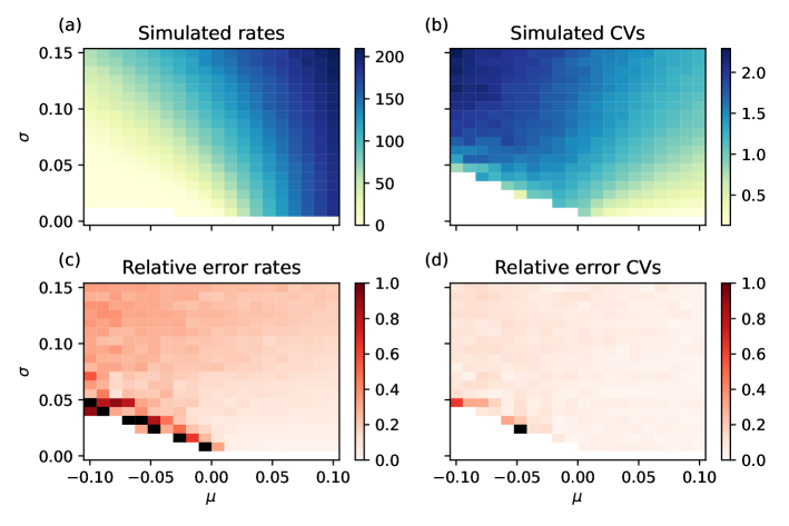
Figure A1: Validity of firing rate and CV prediction for single LIF neuron with instantaneous synapses provided with two independent Poisson inputs. (a) Simulated rates and (b) simulated CVs at given mean input $\mu$ and input variance $\sigma^{2}$. (c) Relative error $\epsilon=\left|\nu_{\mathrm{sim}}-\nu_{\mathrm{thy}}\right|/\nu_{\mathrm{sim}}$ of rate and (d) relative error of CV prediction using Eq. (3) and Eq. (4). Black pixels denote error values larger than $1.00$.

The estimation of covariances presented in this paper relies on the proper estimation of firing rates and CVs, for which we employ Eq. (3) and Eq. (4) [42]. However, these formulae have their own limitations, and they do not yield good estimates in all parameter regimes, as shown in Fig. A1 and Fig. A2a and b. Because the estimates for firing rates and CVs are used to calculate the effective connectivity matrix and noise strength, a poor estimate has a direct impact on the covariance estimation.

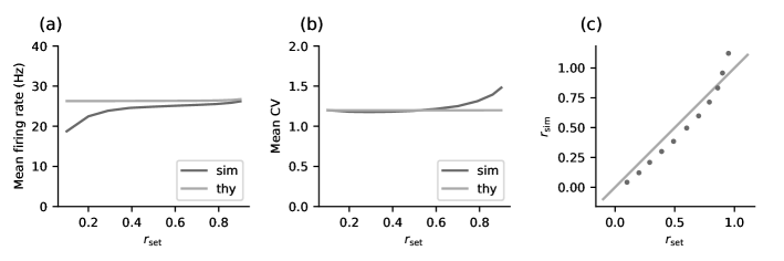
Figure A2: Prediction accuracy of spiking network simulation properties. Predicted and measured (a) mean firing rates and (b) mean CVs at different spectral radii. (c) Set spectral radius $r_{\mathrm{set}}$ vs. measured spectral radius $r_{\mathrm{sim}}$.

Furthermore, the quality of the rate estimates affects how closely the simulated network matches its analytical counterpart due to the way we set the parameters for the simulation: We fix mean and variance of the single neuron input, and therefore their firing rates $\boldsymbol{\nu}_{\mathrm{set}}$, and adjust the external input to set the spectral radius $r$, which we estimate using the result of Rajan and Abbott [69] for random Bernoulli E-I networks

$$r_{\mathrm{set}}=\sqrt{w_{\mathrm{eff,E}}^{2}\left(\boldsymbol{v}_{\mathrm{set}}\right)p\left(1-p\right)N_{\mathrm{E}}+w_{\mathrm{eff,I}}^{2}\left(\boldsymbol{v}_{\mathrm{set}}\right)p\left(1-p\right)N_{\mathrm{I}}}\,,$$

with connection probability $p$. The effective weights $w_{\mathrm{eff,E}}\left(\boldsymbol{\nu}\right)$, $w_{\mathrm{eff,I}}\left(\boldsymbol{\nu}\right)$ are computed using Eq. (6). Once we simulated the network, we can measure the firing rates, extract the connectivity matrix, and compute the effective connectivity matrix realized in the simulation. Its largest eigenvalue determines the spectral radius $r_{\mathrm{sim}}$. A comparison of $r_{\mathrm{set}}$ and $r_{\mathrm{sim}}$ is shown in Fig. A2c. They do not coincide perfectly, which is a direct result of the unreliable estimation of the firing rates, which are slightly overestimated by the theory (see Fig. 2a, Fig. A2a, and Fig. A4a, d, and g). To make sure the simulated network is always in a linearly stable regime, we restrict our analysis to spectral radii $r_{\mathrm{set}}\leq 0.90$, for which $r_{\mathrm{sim}}\leq 0.94$.

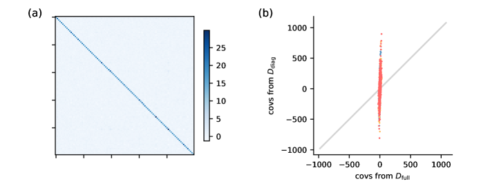
Figure A3: Noise strength properties. (a) First 100 entries of $\boldsymbol{D}_{\mathrm{full}}$ computed from simulated covariances. (b) Comparison of covariances computed using $\boldsymbol{D}_{\mathrm{full}}$ and using $\boldsymbol{D}_{\mathrm{diag}}=\mathrm{diag}\left(\boldsymbol{D}_{\mathrm{full}}\right)$.

We estimate the noise strength $\boldsymbol{D}$ by computing the variances using Eq. (10), assuming that $\boldsymbol{D}$ is diagonal, and inverting Eq. (9) which yields Eq. (11). First of all, the equation for the variances Eq. (10) relies on the assumption that the spike trains are well described by renewal processes [50]. Therefore, the noise strength estimate is reliable only if the spike trains are not too bursty. However, even for networks with $CV\approx 1$ we observed that for large spectral radii this approach of estimating the noise strength can yield negative values for $\boldsymbol{D}$, which has no physical interpretation. Measuring the covariances in a simulation and inverting Eq. (9) without restricting $\boldsymbol{D}$ to be diagonal, yields a matrix that seems to be almost diagonal, shown in Fig. A3a. Setting the off-diagonal elements to zero and using the result to compute the covariances via Eq. (9), however, reveals that the off-diagonal contribution cannot be neglected (Fig. A3b), which means that the external noise sources do have to be correlated to explain the observed covariance. In cases in which the lowest eigenvalue of $\boldsymbol{D}_{\mathrm{full}}$ is negative, we conclude that it is not possible to find a physical linear system (positive definite $\boldsymbol{D}$) that explains the individual pair-wise covariances observed in the spiking network simulation with a large spectral radius. Our theoretical predictions for the mean and variance of cross-covariances, Eq. (22) and Eq. (III.2), based on $\boldsymbol{D}$ computed with Eq. (11) and its averaged analog Eq. (32), nevertheless yield quantitatively matching results with respect to the spiking network simulations also in this regime (Fig. 4), because, as we show in Fig. A5, the results only depend on the average of $\boldsymbol{D}$. The theory based on the statistics of connections is therefore found to be more robust than the theory based on individual connectivity realizations.

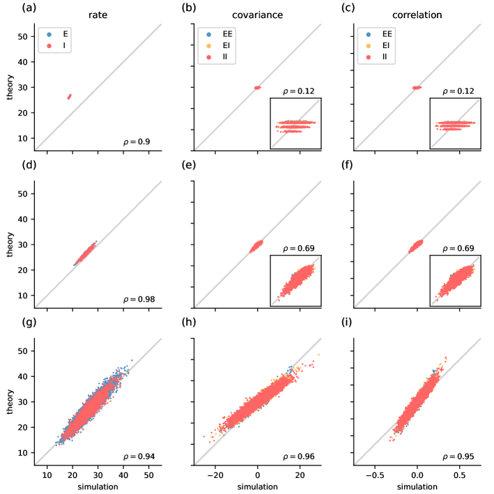
Figure A4: Simulation results vs. theoretical estimates for E-I networks with three different spectral radii $r=0.10$ (a, b, c), $r=0.49$ (d, e, f), $r=0.90$ (g, h, i). $\rho$ denotes the Pearson correlation coefficient. (a, d, g) Firing rates. (b, e, h) Covariances. (c, f, i) Correlation coefficients. The insets show a closer look at the data points.

Finally, simulations have one major limitation: their finite simulation time, which results in a biased estimation of the covariances at the single neuron level. As seen in Fig. A4b, c, e, f, h, and i, there is some variance in the simulations that is not explained by the theory. This variance is caused by the finite simulation time and vanishes for longer simulations. The relative unexplained variance is larger for small spectral radii, since the firing rates of the neurons are slightly smaller in these networks leading to poorer estimation of covariances, and overall the covariances are smaller for small spectral radii.

E Derivation of moment generating function

As discussed in Section II, in absence of correlated external input and in the regime of low average covariances, covariances can be understood in linear response theory [31], where the dynamical equation of LIF neurons describes a model network of Ornstein-Uhlenbeck processes Eq. (5). Grytskyy et al. [31] further showed that the relation Eq. (9) between time-lag integrated covariances and effective connections is independent of the particular filter kernel $h(t)$ and whether noise is injected in the input or output of neurons. Therefore, we here for simplicity choose Gaussian white noise in the input and $h(t)$ to be an exponential kernel with unit time constant. The stochastic differential equation becomes

$$\mathrm{d}\boldsymbol{x}(t)=-\boldsymbol{x}(t)\mathrm{d}t+\boldsymbol{W}\boldsymbol{x}(t)\mathrm{d}t+\mathrm{d}\boldsymbol{\xi}(t)\,,$$ (40)

with generating functional [7]

$$Z\left(\boldsymbol{j}\right)= \int\mathcal{D}\boldsymbol{x}\int\mathcal{D}\widetilde{\boldsymbol{x}}\,\exp\left[\widetilde{\boldsymbol{x}}^{\mathrm{T}}\left(\partial_{t}+1-\boldsymbol{W}\right)\boldsymbol{x}+\frac{D}{2}\widetilde{\boldsymbol{x}}^{\mathrm{T}}\widetilde{\boldsymbol{x}}+\boldsymbol{j}^{\mathrm{T}}\boldsymbol{x}\right]\,.$$

The latter can easily be interpreted in Fourier domain due to the linearity of Eq. (40) and the invariance of scalar products under unitary transforms

$$Z\left(\boldsymbol{J}\right)= \int\mathcal{D}\boldsymbol{X}\int\mathcal{D}\widetilde{\boldsymbol{X}}\,\exp\left[\widetilde{\boldsymbol{X}}^{\mathrm{T}}\left(\mathrm{i}\omega+1-\boldsymbol{W}\right)\boldsymbol{X}+\frac{D}{2}\widetilde{\boldsymbol{X}}^{\mathrm{T}}\widetilde{\boldsymbol{X}}+\boldsymbol{J}^{\mathrm{T}}\boldsymbol{X}\right]\,,$$

with Fourier transformed variables denoted by capital letters. The scalar product in frequency domain reads $\widetilde{\boldsymbol{X}}^{\mathrm{T}}\widetilde{\boldsymbol{X}}=\sum_{j}\int\mathrm{d}\omega\,\widetilde{X}_{j}(-\omega)X_{j}(\omega)$. The generating functional factorizes into generating functions for each frequency $\omega$. As we use Eq. (8) to calculate the time-lag integrated covariances, we only require the zero frequency components $\boldsymbol{X}\left(0\right)$. In the following, we will therefore only discuss zero frequency and omit the frequency argument, i.e. we write $\boldsymbol{X}\equiv\boldsymbol{X}\left(0\right)$ and correspondingly for sources $\boldsymbol{J}$. After integrating over all non-zero frequencies, we obtain the generating function for zero frequency

$$Z\left(\boldsymbol{J}\right)= \lambda\int\mathcal{D}\boldsymbol{X}\int\mathcal{D}\widetilde{\boldsymbol{X}}\,\exp\left[\widetilde{\boldsymbol{X}}^{\mathrm{T}}\left(\boldsymbol{1}-\boldsymbol{W}\right)\boldsymbol{X}+\frac{D}{2}\widetilde{\boldsymbol{X}}^{\mathrm{T}}\widetilde{\boldsymbol{X}}+\boldsymbol{J}^{\mathrm{T}}\boldsymbol{X}\right]\,,$$ (41)

with the single-frequency scalar product defined as $\widetilde{\boldsymbol{X}}^{\mathrm{T}}\widetilde{\boldsymbol{X}}=\sum_{j}\widetilde{X}_{j}\widetilde{X}_{j}$, integration measures $\int\mathcal{D}\boldsymbol{X}=\prod_{j}\int_{-\infty}^{\infty}\mathrm{d}X_{j}$ and $\int\mathcal{D}\widetilde{\boldsymbol{X}}=\prod_{j}\frac{1}{2\pi\mathrm{i}}\int_{-\mathrm{i}\infty}^{\mathrm{i}\infty}\mathrm{d}\widetilde{X}_{j}$, and normalization prefactor $\lambda$. We introduce another source variable $\widetilde{\boldsymbol{J}}$ so that later we can also compute correlators that include $\widetilde{\boldsymbol{X}}$

$$Z\left(\boldsymbol{J},\widetilde{\boldsymbol{J}}\right)= \lambda\int\mathcal{D}\boldsymbol{X}\int\mathcal{D}\widetilde{\boldsymbol{X}}\,\exp\left[\widetilde{\boldsymbol{X}}^{\mathrm{T}}\left(\boldsymbol{1}-\boldsymbol{W}\right)\boldsymbol{X}+\frac{D}{2}\widetilde{\boldsymbol{X}}^{\mathrm{T}}\widetilde{\boldsymbol{X}}+\boldsymbol{J}^{\mathrm{T}}\boldsymbol{X}+\widetilde{\boldsymbol{J}}^{\mathrm{T}}\widetilde{\boldsymbol{X}}\right]\,.$$

The Gaussian integrals are solved as follows

$$Z\left(\boldsymbol{J},\widetilde{\boldsymbol{J}}\right) =\lambda\prod_{i}\int_{-\infty}^{\infty}\mathrm{d}X_{i}\prod_{j}\frac{1}{2\pi\mathrm{i}}\int_{-\mathrm{i}\infty}^{\mathrm{i}\infty}\mathrm{d}\widetilde{X}_{j}\exp\left[\widetilde{\boldsymbol{X}}^{\mathrm{T}}\left(\boldsymbol{1}-\boldsymbol{W}\right)\boldsymbol{X}+\frac{D}{2}\widetilde{\boldsymbol{X}}^{\mathrm{T}}\widetilde{\boldsymbol{X}}+\boldsymbol{J}^{\mathrm{T}}\boldsymbol{X}+\widetilde{\boldsymbol{J}}^{\mathrm{T}}\widetilde{\boldsymbol{X}}\right]$$

$$=\lambda\prod_{i}\int_{-\infty}^{\infty}\mathrm{d}X_{i}\prod_{j}\frac{1}{2\pi}\int_{-\infty}^{\infty}\mathrm{d}\widetilde{X}_{j}\exp\left[\mathrm{i}\widetilde{\boldsymbol{X}}^{\mathrm{T}}\left(\boldsymbol{1}-\boldsymbol{W}\right)\boldsymbol{X}-\frac{D}{2}\widetilde{\boldsymbol{X}}^{\mathrm{T}}\widetilde{\boldsymbol{X}}+\boldsymbol{J}^{\mathrm{T}}\boldsymbol{X}+\mathrm{i}\widetilde{\boldsymbol{J}}^{\mathrm{T}}\widetilde{\boldsymbol{X}}\right]$$

$$=\lambda\left(\frac{1}{2\pi}\right)^{N}\prod_{i}\int_{-\infty}^{\infty}\mathrm{d}X_{i}\prod_{j}\int_{-\infty}^{\infty}\mathrm{d}\widetilde{X}_{j}\exp\left[-\frac{1}{2}\left(\boldsymbol{X}^{\mathrm{T}},\widetilde{\boldsymbol{X}}^{\mathrm{T}}\right)\left(\begin{array}[]{cc}0&-\mathrm{i}\left(\boldsymbol{1}-\boldsymbol{W}^{\mathrm{T}}\right)\\ -\mathrm{i}\left(\boldsymbol{1}-\boldsymbol{W}\right)&D\end{array}\right)\left(\begin{array}[]{c}\boldsymbol{X}\\ \widetilde{\boldsymbol{X}}\end{array}\right)+\left(\boldsymbol{J}^{\mathrm{T}},\mathrm{i}\widetilde{\boldsymbol{J}}^{\mathrm{T}}\right)\left(\begin{array}[]{c}\boldsymbol{X}\\ \widetilde{\boldsymbol{X}}\end{array}\right)\right]$$

$$=\lambda\left(\frac{1}{2\pi}\right)^{N}\sqrt{\frac{\left(2\pi\right)^{2N}}{\det\left(\begin{array}[]{cc}0&-\mathrm{i}\left(\boldsymbol{1}-\boldsymbol{W}^{\mathrm{T}}\right)\\ -\mathrm{i}\left(\boldsymbol{1}-\boldsymbol{W}\right)&D\end{array}\right)}}\exp\left[\frac{1}{2}\left(\boldsymbol{J}^{\mathrm{T}},\mathrm{i}\widetilde{\boldsymbol{J}}^{\mathrm{T}}\right)\left(\begin{array}[]{cc}0&-\mathrm{i}\left(\boldsymbol{1}-\boldsymbol{W}^{\mathrm{T}}\right)\\ -\mathrm{i}\left(\boldsymbol{1}-\boldsymbol{W}\right)&D\end{array}\right)^{-1}\left(\begin{array}[]{c}\boldsymbol{J}\\ \mathrm{i}\widetilde{\boldsymbol{J}}\end{array}\right)\right]$$

$$=\frac{\lambda}{\sqrt{\det\left(\begin{array}[]{cc}0&-\mathrm{i}\left(\boldsymbol{1}-\boldsymbol{W}^{\mathrm{T}}\right)\\ -\mathrm{i}\left(\boldsymbol{1}-\boldsymbol{W}\right)&D\end{array}\right)}}\exp\left[\frac{1}{2}\left(\boldsymbol{J}^{\mathrm{T}},\mathrm{i}\widetilde{\boldsymbol{J}}^{\mathrm{T}}\right)\left(\begin{array}[]{cc}\left(\boldsymbol{1}-\boldsymbol{W}\right)^{-1}D\left(\boldsymbol{1}-\boldsymbol{W}^{\mathrm{T}}\right)^{-1}&\mathrm{i}\left(\boldsymbol{1}-\boldsymbol{W}\right)^{-1}\\ \mathrm{i}\left(\boldsymbol{1}-\boldsymbol{W}^{\mathrm{T}}\right)^{-1}&0\end{array}\right)\left(\begin{array}[]{c}\boldsymbol{J}\\ \mathrm{i}\widetilde{\boldsymbol{J}}\end{array}\right)\right]$$

$$=\frac{\lambda}{\sqrt{\det\left(\begin{array}[]{cc}0&-\mathrm{i}\left(\boldsymbol{1}-\boldsymbol{W}^{\mathrm{T}}\right)\\ -\mathrm{i}\left(\boldsymbol{1}-\boldsymbol{W}\right)&D\end{array}\right)}}\exp\left[\frac{1}{2}\left(\boldsymbol{J}^{\mathrm{T}},\widetilde{\boldsymbol{J}}^{\mathrm{T}}\right)\left(\begin{array}[]{cc}\left(\boldsymbol{1}-\boldsymbol{W}\right)^{-1}D\left(\boldsymbol{1}-\boldsymbol{W}^{\mathrm{T}}\right)^{-1}&-\left(\boldsymbol{1}-\boldsymbol{W}\right)^{-1}\\ -\left(\boldsymbol{1}-\boldsymbol{W}^{\mathrm{T}}\right)^{-1}&0\end{array}\right)\left(\begin{array}[]{c}\boldsymbol{J}\\ \widetilde{\boldsymbol{J}}\end{array}\right)\right]\,.$$

The identity matrix and the matrix of ones commute, therefore we can use $\det\left(\begin{array}[]{cc}A&B\\ C&D\end{array}\right)=\det(AD-BC)$, and we get

$$\det\left(\begin{array}[]{cc}0&-\mathrm{i}\left(\boldsymbol{1}-\boldsymbol{W}^{\mathrm{T}}\right)\\ -\mathrm{i}\left(\boldsymbol{1}-\boldsymbol{W}\right)&D\end{array}\right) =\det\left[-\mathrm{i}^{2}\left(\boldsymbol{1}-\boldsymbol{W}^{\mathrm{T}}\right)\left(\boldsymbol{1}-\boldsymbol{W}\right)\right]$$

$$=\left[\det\left(\boldsymbol{1}-\boldsymbol{W}\right)\right]^{2}\,.$$

The normalization condition $Z\left(\boldsymbol{J}=0\right)=1$ yields $\lambda=\left|\det\left(1-\boldsymbol{W}\right)\right|$, and the generating function becomes

$$Z\left(\boldsymbol{J},\widetilde{\boldsymbol{J}}\right) =\exp\left[\frac{1}{2}\left(\boldsymbol{J}^{\mathrm{T}},\widetilde{\boldsymbol{J}}^{\mathrm{T}}\right)\left(\begin{array}[]{cc}\left(\boldsymbol{1}-\boldsymbol{W}\right)^{-1}D\left(\boldsymbol{1}-\boldsymbol{W}^{\mathrm{T}}\right)^{-1}&-\left(\boldsymbol{1}-\boldsymbol{W}\right)^{-1}\\ -\left(\boldsymbol{1}-\boldsymbol{W}\right)^{-\mathrm{T}}&0\end{array}\right)\left(\begin{array}[]{c}\boldsymbol{J}\\ \widetilde{\boldsymbol{J}}\end{array}\right)\right]\,,$$

or

$$Z\left(\boldsymbol{J},\widetilde{\boldsymbol{J}}=0\right) =\left|\det\left(1-\boldsymbol{W}\right)\right|\int\mathcal{D}\boldsymbol{X}\int\mathcal{D}\widetilde{\boldsymbol{X}}\,\exp\left[\widetilde{\boldsymbol{X}}^{\mathrm{T}}\left(\boldsymbol{1}-\boldsymbol{W}\right)\boldsymbol{X}+\frac{D}{2}\widetilde{\boldsymbol{X}}^{\mathrm{T}}\widetilde{\boldsymbol{X}}+\boldsymbol{J}^{\mathrm{T}}\boldsymbol{X}\right]$$ (42)

$$=\exp\left(\frac{1}{2}\boldsymbol{J}^{\mathrm{T}}\left(\boldsymbol{1}-\boldsymbol{W}\right)^{-1}\boldsymbol{D}\left(\boldsymbol{1}-\boldsymbol{W}\right)^{-\mathrm{T}}\boldsymbol{J}\right)\,,$$

respectively. We obtain the time-lag integrated covariances

$$C_{ij} =\left\langle X_{i}X_{j}\right\rangle$$

$$=\left.\frac{\mathrm{\partial}}{\partial J_{i}}\frac{\mathrm{\partial}}{\partial J_{j}}Z\left(\boldsymbol{J},\widetilde{\boldsymbol{J}}\right)\right|_{\boldsymbol{J},\widetilde{\boldsymbol{J}}=0}$$

$$=\left[\left(\boldsymbol{1}-\boldsymbol{W}\right)^{-1}\boldsymbol{D}\left(\boldsymbol{1}-\boldsymbol{W}\right)^{-\mathrm{T}}\right]_{ij}\,.$$

F Saddle points and correlators of activity fields

The saddle points $\boldsymbol{Q}^{*},\widetilde{\boldsymbol{Q}}^{*}$ are given by $\left.\frac{\partial}{\partial Q_{i}}S\left(\boldsymbol{Q},\widetilde{\boldsymbol{Q}}\right)\right|_{\boldsymbol{Q}^{*},\widetilde{\boldsymbol{Q}}^{*}}=0$ and $\left.\frac{\partial}{\partial\widetilde{Q}_{i}}S\left(\boldsymbol{Q},\widetilde{\boldsymbol{Q}}\right)\right|_{\boldsymbol{Q}^{*},\widetilde{\boldsymbol{Q}}^{*}}=0$, which yield

$$Q_{i}^{*} = \frac{1}{N}\sum_{j}\Delta_{ij}\left\langle X_{j}X_{j}\right\rangle_{\boldsymbol{Q}^{*},\widetilde{\boldsymbol{Q}}^{*}}\,,$$

$$\widetilde{Q}_{i}^{*} = \frac{1}{2N}\left\langle\widetilde{X}_{i}\widetilde{X}_{i}\right\rangle_{\boldsymbol{Q}^{*},\widetilde{\boldsymbol{Q}}^{*}}\,,$$

including correlators evaluated at the saddle point $\boldsymbol{Q}^{*},\widetilde{\boldsymbol{Q}}^{*}$. To evaluate them, we need to solve the Gaussian integral in Eq. (III.1)

$$\widetilde{Z}\left(\boldsymbol{J},\widetilde{\boldsymbol{J}}\right) = \int\mathcal{D}\boldsymbol{X}\int\mathcal{D}\widetilde{\boldsymbol{X}}\,\exp\left[\widetilde{\boldsymbol{X}}^{\mathrm{T}}\left(\boldsymbol{1}-\boldsymbol{M}\right)\boldsymbol{X}+\frac{1}{2}\widetilde{\boldsymbol{X}}^{\mathrm{T}}\left[\boldsymbol{D}+\mathrm{diag}\left(\boldsymbol{Q}\right)\right]\widetilde{\boldsymbol{X}}+\boldsymbol{X}^{\mathrm{T}}\mathrm{diag}\left(\widetilde{\boldsymbol{Q}}^{\mathrm{T}}\boldsymbol{\Delta}\right)\boldsymbol{X}+\boldsymbol{J}^{\mathrm{T}}\boldsymbol{X}+\widetilde{\boldsymbol{J}}^{\mathrm{T}}\widetilde{\boldsymbol{X}}\right]\,,$$

where we added the additional source term $\widetilde{\boldsymbol{J}}^{\mathrm{T}}\widetilde{\boldsymbol{X}}$ to allow for the calculation of correlators including $\widetilde{\boldsymbol{X}}$. We can rewrite the equation as

$$\widetilde{Z}\left(\boldsymbol{J}\right) =\int\mathcal{D}\boldsymbol{Z}\,\exp\left[-\frac{1}{2}\boldsymbol{Z}^{\mathrm{T}}\boldsymbol{A}\boldsymbol{Z}+\boldsymbol{B}^{\mathrm{T}}\boldsymbol{Z}\right]$$

$$=\left(2\pi\right)^{-N}\sqrt{\frac{\left(2\pi\right)^{2n}}{\mathrm{det}\boldsymbol{A}}}\exp\left(\frac{1}{2}\boldsymbol{B}^{T}\boldsymbol{A}^{-1}\boldsymbol{B}\right)$$

$$=\frac{1}{\sqrt{\mathrm{det}\boldsymbol{A}}}\exp\left(\frac{1}{2}\boldsymbol{B}^{T}\boldsymbol{A}^{-1}\boldsymbol{B}\right)\,,$$

using

$$\boldsymbol{Z} = \left(\begin{array}[]{c}\boldsymbol{X}\\ \widetilde{\boldsymbol{X}}\end{array}\right)\,,\quad\boldsymbol{B}=\left(\begin{array}[]{c}\boldsymbol{J}\\ \mathrm{i}\widetilde{\boldsymbol{J}}\end{array}\right)\,,$$

$$\boldsymbol{A} = \left(\begin{array}[]{cc}-2\mathrm{diag}\left(\widetilde{\boldsymbol{Q}}^{\mathrm{T}}\boldsymbol{\Delta}\right)&-\mathrm{i}\left(\boldsymbol{1}-\boldsymbol{M}\right)^{\mathrm{T}}\\ -\mathrm{i}\left(\boldsymbol{1}-\boldsymbol{M}\right)&\left[\boldsymbol{D}+\mathrm{diag}\left(\boldsymbol{Q}\right)\right]\end{array}\right)\,,$$

where the prefactor $\left(2\pi\right)^{-N}$ came from the integration measure $\mathcal{D}\widetilde{\boldsymbol{X}}$ , such that

$$\boldsymbol{A}_{11}^{-1} = \left\{-2\mathrm{diag}\left(\widetilde{\boldsymbol{Q}}^{\mathrm{T}}\boldsymbol{\Delta}\right)+\left(\boldsymbol{1}-\boldsymbol{M}\right)^{\mathrm{T}}\left[\boldsymbol{D}+\mathrm{diag}\left(\boldsymbol{Q}\right)\right]^{-1}\left(\boldsymbol{1}-\boldsymbol{M}\right)\right\}^{-1}\,,$$

$$\boldsymbol{A}_{12}^{-1} = \mathrm{i}\left\{-2\mathrm{diag}\left(\widetilde{\boldsymbol{Q}}^{\mathrm{T}}\boldsymbol{\Delta}\right)+\left(\boldsymbol{1}-\boldsymbol{M}\right)^{\mathrm{T}}\left[\boldsymbol{D}+\mathrm{diag}\left(\boldsymbol{Q}\right)\right]^{-1}\left(\boldsymbol{1}-\boldsymbol{M}\right)\right\}^{-1}\left(\boldsymbol{1}-\boldsymbol{M}\right)^{\mathrm{T}}\left[\boldsymbol{D}+\mathrm{diag}\left(\boldsymbol{Q}\right)\right]^{-1}\,,$$

$$\boldsymbol{A}_{21}^{-1} = \mathrm{i}\left[\boldsymbol{D}+\mathrm{diag}\left(\boldsymbol{Q}\right)\right]^{-1}\left(\boldsymbol{1}-\boldsymbol{M}\right)\left\{-2\mathrm{diag}\left(\widetilde{\boldsymbol{Q}}^{\mathrm{T}}\boldsymbol{\Delta}\right)+\left(\boldsymbol{1}-\boldsymbol{M}\right)^{\mathrm{T}}\left[\boldsymbol{D}+\mathrm{diag}\left(\boldsymbol{Q}\right)\right]^{-1}\left(\boldsymbol{1}-\boldsymbol{M}\right)\right\}^{-1}\,,$$

$$\boldsymbol{A}_{22}^{-1} = \left[\boldsymbol{D}+\mathrm{diag}\left(\boldsymbol{Q}\right)\right]^{-1}$$

$$-\left[\boldsymbol{D}+\mathrm{diag}\left(\boldsymbol{Q}\right)\right]^{-1}\left(\boldsymbol{1}-\boldsymbol{M}\right)\left\{-2\mathrm{diag}\left(\widetilde{\boldsymbol{Q}}^{\mathrm{T}}\boldsymbol{\Delta}\right)+\left(\boldsymbol{1}-\boldsymbol{M}\right)^{\mathrm{T}}\left[\boldsymbol{D}+\mathrm{diag}\left(\boldsymbol{Q}\right)\right]^{-1}\left(\boldsymbol{1}-\boldsymbol{M}\right)\right\}^{-1}\left(\boldsymbol{1}-\boldsymbol{M}\right)^{\mathrm{T}}\left[\boldsymbol{D}+\mathrm{diag}\left(\boldsymbol{Q}\right)\right]^{-1}\,.$$

Deriving the normalized moment generating function $Z\left(\boldsymbol{J},\widetilde{\boldsymbol{J}}\right)=\widetilde{Z}\left(\boldsymbol{J},\widetilde{\boldsymbol{J}}\right)/\widetilde{Z}\left(0,0\right)$ twice with respect to $\widetilde{\boldsymbol{J}}$ yields

$$\widetilde{\boldsymbol{Q}}^{*} = \frac{1}{2N}\left\langle\widetilde{\boldsymbol{X}}\widetilde{\boldsymbol{X}}^{\mathrm{T}}\right\rangle_{\boldsymbol{Q}^{*},\widetilde{\boldsymbol{Q}}^{*}}$$

$$= \frac{1}{2N}A_{22}^{-1}$$

$$= \frac{1}{2N}\biggl{(}\left[\boldsymbol{D}+\mathrm{diag}\left(\boldsymbol{Q}\right)\right]^{-1}$$

$$-\left[\boldsymbol{D}+\mathrm{diag}\left(\boldsymbol{Q}\right)\right]^{-1}\left(\boldsymbol{1}-\boldsymbol{M}\right)\left\{-2\mathrm{diag}\left(\widetilde{\boldsymbol{Q}}^{\mathrm{T}}\boldsymbol{\Delta}\right)+\left(\boldsymbol{1}-\boldsymbol{M}\right)^{\mathrm{T}}\left[\boldsymbol{D}+\mathrm{diag}\left(\boldsymbol{Q}\right)\right]^{-1}\left(\boldsymbol{1}-\boldsymbol{M}\right)\right\}^{-1}\left(\boldsymbol{1}-\boldsymbol{M}\right)^{\mathrm{T}}\left[\boldsymbol{D}+\mathrm{diag}\left(\boldsymbol{Q}\right)\right]^{-1}\biggr{)}\,,$$

which is solved by $\widetilde{\boldsymbol{Q}}^{*}=0$. Inserting this results, we find

$$\left\langle\boldsymbol{X}\boldsymbol{X}^{\mathrm{T}}\right\rangle_{\boldsymbol{Q}^{*},\widetilde{\boldsymbol{Q}}^{*}} = \left(\boldsymbol{1}-\boldsymbol{M}\right)^{-1}\left[\boldsymbol{D}+\mathrm{diag}\left(\boldsymbol{Q}\right)\right]\left(\boldsymbol{1}-\boldsymbol{M}\right)^{-\mathrm{T}}\,,$$

$$\left\langle\widetilde{\boldsymbol{X}}\boldsymbol{X}^{\mathrm{T}}\right\rangle_{\boldsymbol{Q}^{*},\widetilde{\boldsymbol{Q}}^{*}} = -\left(\boldsymbol{1}-\boldsymbol{M}\right)^{-\mathrm{T}}\,,$$

$$\left\langle\widetilde{\boldsymbol{X}}\widetilde{\boldsymbol{X}}^{\mathrm{T}}\right\rangle_{\boldsymbol{Q}^{*},\widetilde{\boldsymbol{Q}}^{*}} = 0\,.$$

Inserting the correlators into the saddle-point equations and solving for $\boldsymbol{Q}^{*}$ yields

$$Q_{i}^{*} = \frac{1}{N}\sum_{j,k,l,m}\left(\boldsymbol{1}-\frac{1}{N}\Delta\cdot\boldsymbol{R}\odot\boldsymbol{R}\right)_{ij}^{-1}\Delta_{jk}R_{kl}D_{lm}R_{km}\,,$$ (45)

$$\widetilde{Q}_{i}^{*} = 0\,.$$

with $\boldsymbol{R}=\left(\boldsymbol{1}-\boldsymbol{M}\right)^{-1}$.

The saddle point of the auxiliary fields $\boldsymbol{Q}_{XX}$, $\boldsymbol{Q}_{XY}$, $\boldsymbol{Q}_{YY}$ in the replica-theory are determined by finding the zeros of the first derivative of the action Eq. (25). This yields

$$Q_{XX,i}^{*} = \frac{1}{N}\sum_{j}\Delta_{ij}\left\langle X_{j}X_{j}\right\rangle_{\boldsymbol{Q}^{*},\widetilde{\boldsymbol{Q}}^{*}}=Q_{i}^{*}\,,$$

$$Q_{YY,i}^{*} = \frac{1}{N}\sum_{j}\Delta_{ij}\left\langle Y_{j}Y_{j}\right\rangle_{\boldsymbol{Q}^{*},\widetilde{\boldsymbol{Q}}^{*}}=Q_{i}^{*}\,,$$

$$Q_{XY,i}^{*} = \frac{1}{N}\sum_{j}\Delta_{ij}\left\langle X_{j}Y_{j}\right\rangle_{\boldsymbol{Q}^{*},\widetilde{\boldsymbol{Q}}^{*}}\,,$$

$$\widetilde{Q}_{XX,i}^{*} = \frac{1}{2N}\left\langle\widetilde{X}_{i}\widetilde{X}_{i}\right\rangle_{\boldsymbol{Q}^{*},\widetilde{\boldsymbol{Q}}^{*}}=0\,,$$

$$\widetilde{Q}_{YY,i}^{*} = \frac{1}{2N}\left\langle\widetilde{Y}_{i}\widetilde{Y}_{i}\right\rangle_{\boldsymbol{Q}^{*},\widetilde{\boldsymbol{Q}}^{*}}=0\,,$$

$$\widetilde{Q}_{XY,i}^{*} = \frac{1}{N}\left\langle\widetilde{X}_{i}\widetilde{Y}_{i}\right\rangle_{\boldsymbol{Q}^{*},\widetilde{\boldsymbol{Q}}^{*}}=0\,,$$

and in an analogous fashion to the derivation above, we find

$$\left\langle\boldsymbol{X}\boldsymbol{Y}^{\mathrm{T}}\right\rangle_{\boldsymbol{Q}^{*},\widetilde{\boldsymbol{Q}}^{*}}=\left(\boldsymbol{1}-\boldsymbol{M}\right)^{-1}\mathrm{diag}\left(\boldsymbol{Q}_{XY}^{*}\right)\left(\boldsymbol{1}-\boldsymbol{M}\right)^{-\mathrm{T}}\,.$$

Inserting the latter solution into the saddle point equations again yields a linear self-consistency equation for $\boldsymbol{Q}_{XY}^{*}$ with the solution

$$Q_{XY,i}^{*}=0\,,$$

such that

$$\left\langle\boldsymbol{X}\boldsymbol{Y}^{\mathrm{T}}\right\rangle_{\boldsymbol{Q}^{*},\widetilde{\boldsymbol{Q}}^{*}}=0\,.$$

G Fluctuations around saddle-points

Here we showcase how to perform a fluctuation expansion of the correlator $\left\langle X_{i}Y_{i}\right\rangle_{\boldsymbol{Q},\widetilde{\boldsymbol{Q}}}$ around $\boldsymbol{Q}_{XY}^{*}$ and $\widetilde{\boldsymbol{Q}}_{XY}^{*}$. Other correlators follow analogously. Following the definition in Eq. (24), the correlator is given by

$$\left\langle X_{i}Y_{i}\right\rangle_{\boldsymbol{Q},\widetilde{\boldsymbol{Q}}} =\left.\frac{\partial}{\partial J_{i}}\frac{\partial}{\partial K_{i}}Z_{\boldsymbol{Q},\widetilde{\boldsymbol{Q}}}\left(\boldsymbol{J},\boldsymbol{K}\right)\right|_{\boldsymbol{J},\boldsymbol{K}=0}\,.$$

Now, we expand $Z_{\boldsymbol{Q},\widetilde{\boldsymbol{Q}}}$ around the saddle points

$$Z_{\boldsymbol{Q},\widetilde{\boldsymbol{Q}}}\left(\boldsymbol{J},\boldsymbol{K}\right)\approx Z_{\boldsymbol{Q}^{*},\widetilde{\boldsymbol{Q}}^{*}}\left(\boldsymbol{J},\boldsymbol{K}\right)$$

$$+\sum_{k}\left.\frac{\partial}{\partial Q_{XY,k}}Z_{\boldsymbol{Q},\widetilde{\boldsymbol{Q}}}\left(\boldsymbol{J},\boldsymbol{K}\right)\right|_{\boldsymbol{Q}^{*},\widetilde{\boldsymbol{Q}}^{*}}\left(Q_{XY,k}-Q_{XY,k}^{*}\right)$$

$$+\sum_{k}\left.\frac{\partial}{\partial\widetilde{Q}_{XY,k}}Z_{\boldsymbol{Q},\widetilde{\boldsymbol{Q}}}\left(\boldsymbol{J},\boldsymbol{K}\right)\right|_{\boldsymbol{Q}^{*},\widetilde{\boldsymbol{Q}}^{*}}\left(\widetilde{Q}_{XY,k}-\widetilde{Q}_{XY,k}^{*}\right)\,,$$

and use $Z_{\boldsymbol{Q},\widetilde{\boldsymbol{Q}}}\left(\boldsymbol{J},\boldsymbol{K}\right)=\widetilde{Z}_{\boldsymbol{Q},\widetilde{\boldsymbol{Q}}}\left(\boldsymbol{J},\boldsymbol{K}\right)/\widetilde{Z}_{\boldsymbol{Q},\widetilde{\boldsymbol{Q}}}\left(\boldsymbol{0},\boldsymbol{0}\right)$ to obtain

$$\frac{\partial}{\partial Q_{XY,k}}Z_{\boldsymbol{Q},\widetilde{\boldsymbol{Q}}}\left(\boldsymbol{J},\boldsymbol{K}\right) =\frac{1}{\widetilde{Z}_{\boldsymbol{Q},\widetilde{\boldsymbol{Q}}}\left(\boldsymbol{0},\boldsymbol{0}\right)}\frac{\partial}{\partial Q_{XY,k}}\widetilde{Z}_{\boldsymbol{Q},\widetilde{\boldsymbol{Q}}}\left(\boldsymbol{J},\boldsymbol{K}\right)-\frac{\widetilde{Z}_{\boldsymbol{Q},\widetilde{\boldsymbol{Q}}}\left(\boldsymbol{J},\boldsymbol{K}\right)}{\widetilde{Z}_{\boldsymbol{Q},\widetilde{\boldsymbol{Q}}}\left(\boldsymbol{0},\boldsymbol{0}\right)^{2}}\frac{\partial}{\partial Q_{XY,k}}\widetilde{Z}_{\boldsymbol{Q},\widetilde{\boldsymbol{Q}}}\left(0,0\right)\,.$$ (46)

Using the definition of $\widetilde{Z}_{\boldsymbol{Q},\widetilde{\boldsymbol{Q}}}\left(\boldsymbol{J},\boldsymbol{K}\right)$ in Eq. (25), its derivative is given by

$$\frac{\partial}{\partial Q_{XY,k}}\widetilde{Z}_{\boldsymbol{Q},\widetilde{\boldsymbol{Q}}}\left(\boldsymbol{J},\boldsymbol{K}\right)= \int\mathcal{D}\boldsymbol{X}\int\mathcal{D}\widetilde{\boldsymbol{X}}\int\mathcal{D}\boldsymbol{Y}\int\mathcal{D}\widetilde{\boldsymbol{Y}}\,\widetilde{X}_{k}\widetilde{Y}_{k}$$

$$\times\exp\Big{[} S_{\boldsymbol{Q}_{XX},\widetilde{\boldsymbol{Q}}_{XX}}\left(\boldsymbol{X},\widetilde{\boldsymbol{X}}\right)+S_{\boldsymbol{Q}_{YY},\widetilde{\boldsymbol{Q}}_{YY}}\left(\boldsymbol{Y},\widetilde{\boldsymbol{Y}}\right)+\widetilde{\boldsymbol{X}}^{\mathrm{T}}\mathrm{diag}\left(\boldsymbol{Q}_{XY}\right)\widetilde{\boldsymbol{Y}}+\boldsymbol{X}^{\mathrm{T}}\mathrm{diag}\left(\widetilde{\boldsymbol{Q}}_{XY}^{\mathrm{T}}\boldsymbol{\Delta}\right)\boldsymbol{Y}+\boldsymbol{J}^{\mathrm{T}}\boldsymbol{X}+\boldsymbol{K}^{\mathrm{T}}\boldsymbol{Y}\Big{]}\,,$$

such that normalizing and evaluating at the saddle point and for zero sources yields

$$\left.\frac{\left.\frac{\partial}{\partial J_{i}}\frac{\partial}{\partial K_{i}}\frac{\partial}{\partial Q_{XY,k}}\widetilde{Z}_{\boldsymbol{Q},\widetilde{\boldsymbol{Q}}}\left(\boldsymbol{J},\boldsymbol{K}\right)\right|_{\boldsymbol{J},\boldsymbol{K}=0}}{\widetilde{Z}_{\boldsymbol{Q},\widetilde{\boldsymbol{Q}}}\left(\boldsymbol{0},\boldsymbol{0}\right)}\right|_{\boldsymbol{Q}^{*},\widetilde{\boldsymbol{Q}}^{*}} =\left\langle X_{i}Y_{i}\widetilde{X}_{k}\widetilde{Y}_{k}\right\rangle_{\boldsymbol{Q}^{*},\widetilde{\boldsymbol{Q}}^{*}}\,.$$

The second term on the right hand side of Eq. (46) vanishes at the saddle point and for $\boldsymbol{J}=\boldsymbol{K}=0$

$$\left.\left.\frac{\partial}{\partial J_{i}}\frac{\partial}{\partial K_{i}}\frac{\widetilde{Z}_{\boldsymbol{Q},\widetilde{\boldsymbol{Q}}}\left(\boldsymbol{J},\boldsymbol{K}\right)}{\widetilde{Z}_{\boldsymbol{Q},\widetilde{\boldsymbol{Q}}}\left(\boldsymbol{0},\boldsymbol{0}\right)^{2}}\frac{\partial}{\partial Q_{XY,k}}\widetilde{Z}_{\boldsymbol{Q},\widetilde{\boldsymbol{Q}}}\left(0,0\right)\right|_{\boldsymbol{J},\boldsymbol{K}=0}\right|_{\boldsymbol{Q}^{*},\widetilde{\boldsymbol{Q}}^{*}}=\left\langle X_{i}Y_{i}\right\rangle_{\boldsymbol{Q}^{*},\widetilde{\boldsymbol{Q}}^{*}}\left\langle\widetilde{X}_{k}\widetilde{Y}_{k}\right\rangle_{\boldsymbol{Q}^{*},\widetilde{\boldsymbol{Q}}^{*}}=0\,.$$

The derivative with respect to $\widetilde{Q}_{XY,k}$ can be computed analogously, with $\widetilde{X}_{k}\widetilde{Y}_{k}$ replaced by $\sum_{l}\Delta_{kl}X_{l}Y_{l}$. Therefore, the first order expansion in the replica coupling term reads

$$\left\langle X_{i}Y_{i}\right\rangle_{\boldsymbol{Q},\widetilde{\boldsymbol{Q}}}=\underbrace{\left\langle X_{i}Y_{i}\right\rangle_{\boldsymbol{Q}^{*},\widetilde{\boldsymbol{Q}}^{*}}}_{=0}+\sum_{k}\left\langle X_{i}Y_{i}\widetilde{X}_{k}\widetilde{Y}_{k}\right\rangle_{\boldsymbol{Q}^{*},\widetilde{\boldsymbol{Q}}^{*}}\left(Q_{XY,k}-Q_{XY,k}^{*}\right)+\sum_{k,l}\Delta_{kl}\left\langle X_{i}Y_{i}X_{l}Y_{l}\right\rangle_{\boldsymbol{Q}^{*},\widetilde{\boldsymbol{Q}}^{*}}\left(\widetilde{Q}_{XY,k}-\widetilde{Q}_{XY,k}^{*}\right)\,,$$ (47)

which we use in Eq. (28).

H Correlators of auxiliary fields

We consider the Gaussian approximation of $p\left(\boldsymbol{Q},\widetilde{\boldsymbol{Q}}\right)$ with

$$\mathcal{S}\left(\boldsymbol{Q},\widetilde{\boldsymbol{Q}}\right)=\mathcal{S}\left(\boldsymbol{Q}^{*},\widetilde{\boldsymbol{Q}}^{*}\right)+\frac{1}{2}\left(\delta\boldsymbol{Q}_{XY},\delta\widetilde{\boldsymbol{Q}}_{XY}\right)\boldsymbol{\mathcal{S}}^{(2)}\left(\begin{array}[]{c}\delta\boldsymbol{Q}_{XY}\\ \delta\widetilde{\boldsymbol{Q}}_{XY}\end{array}\right)\,,$$

where $\boldsymbol{S}^{(2)}$ contains the second derivatives with respect to the auxiliary fields

$$\boldsymbol{S}^{(2)}=\left(\begin{array}[]{cc}\left.\frac{\partial\mathcal{S}\left(\boldsymbol{Q},\widetilde{\boldsymbol{Q}}\right)}{\partial\boldsymbol{Q}_{XY}\partial\boldsymbol{Q}_{XY}}\right|_{\boldsymbol{Q}^{*},\widetilde{\boldsymbol{Q}}^{*}}&\left.\frac{\partial\mathcal{S}\left(\boldsymbol{Q},\widetilde{\boldsymbol{Q}}\right)}{\partial\boldsymbol{Q}_{XY}\partial\widetilde{\boldsymbol{Q}}_{XY}}\right|_{\boldsymbol{Q}^{*},\widetilde{\boldsymbol{Q}}^{*}}\\ \left.\frac{\partial\mathcal{S}\left(\boldsymbol{Q},\widetilde{\boldsymbol{Q}}\right)}{\partial\widetilde{\boldsymbol{Q}}_{XY}\partial\boldsymbol{Q}_{XY}}\right|_{\boldsymbol{Q}^{*},\widetilde{\boldsymbol{Q}}^{*}}&\left.\frac{\partial\mathcal{S}\left(\boldsymbol{Q},\widetilde{\boldsymbol{Q}}\right)}{\partial\widetilde{\boldsymbol{Q}}_{XY}\partial\widetilde{\boldsymbol{Q}}_{XY}}\right|_{\boldsymbol{Q}^{*},\widetilde{\boldsymbol{Q}}^{*}}\end{array}\right)\,,$$

with

$$\mathcal{S}_{11,ij}^{(2)} = 0$$

$$\mathcal{S}_{12,ij}^{(2)} = N\delta_{ij}-\sum_{k}\Delta_{jk}\left\langle\widetilde{X}_{i}\widetilde{Y}_{i}X_{k}Y_{k}\right\rangle_{\boldsymbol{Q}^{*},\widetilde{\boldsymbol{Q}}^{*}}=N\delta_{ij}-\sum_{k}\Delta_{jk}R_{ki}^{2}$$

$$\mathcal{S}_{21,ij}^{(2)} = N\delta_{ij}-\sum_{k}\Delta_{ik}\left\langle\widetilde{X}_{j}\widetilde{Y}_{j}X_{k}Y_{k}\right\rangle_{\boldsymbol{Q}^{*},\widetilde{\boldsymbol{Q}}^{*}}=N\delta_{ij}-\sum_{k}\Delta_{ik}R_{kj}^{2}$$

$$\mathcal{S}_{22,ij}^{(2)} = -\sum_{k,l}\Delta_{ik}\Delta_{jl}\left\langle X_{k}Y_{k}X_{l}Y_{l}\right\rangle_{\boldsymbol{Q}^{*},\widetilde{\boldsymbol{Q}}^{*}}=-\sum_{k,l}\Delta_{ik}\Delta_{jl}\left\langle X_{k}X_{l}\right\rangle_{\boldsymbol{Q}^{*},\widetilde{\boldsymbol{Q}}^{*}}\left\langle Y_{k}Y_{l}\right\rangle_{\boldsymbol{Q}^{*},\widetilde{\boldsymbol{Q}}^{*}}\,.$$

Using

$$\boldsymbol{\mathcal{S}}^{(2)}=\left(\begin{array}[]{cc}0&\boldsymbol{\mathcal{S}}_{21}^{(2)\mathrm{T}}\\ \boldsymbol{\mathcal{S}}_{21}^{(2)}&\boldsymbol{\mathcal{S}}_{22}^{(2)}\end{array}\right)\,,\quad\left(\boldsymbol{\mathcal{S}}^{(2)}\right)^{-1}=\left(\begin{array}[]{cc}-\boldsymbol{\mathcal{S}}_{21}^{(2)-1}\boldsymbol{\mathcal{S}}_{22}^{(2)}\boldsymbol{\mathcal{S}}_{21}^{(2)-\mathrm{T}}&\boldsymbol{\mathcal{S}}_{21}^{(2)-1}\\ \boldsymbol{\mathcal{S}}_{21}^{(2)-\mathrm{T}}&0\end{array}\right)\,,$$

we find

$$\left\langle\delta\boldsymbol{Q}_{XY}\delta\boldsymbol{Q}_{XY}^{\mathrm{T}}\right\rangle = -\boldsymbol{\mathcal{S}}_{21}^{(2)-1}\boldsymbol{\mathcal{S}}_{22}^{(2)}\boldsymbol{\mathcal{S}}_{21}^{(2)-\mathrm{T}}$$

$$= \frac{1}{N^{2}}\left[\boldsymbol{1}-\frac{1}{N}\boldsymbol{\Delta}\cdot\left(\boldsymbol{R}\odot\boldsymbol{R}\right)\right]^{-1}\boldsymbol{\Delta}\left\langle\boldsymbol{X}\boldsymbol{X}^{\mathrm{T}}\right\rangle_{\boldsymbol{Q}^{*},\widetilde{\boldsymbol{Q}}^{*}}\odot\left\langle\boldsymbol{X}\boldsymbol{X}^{\mathrm{T}}\right\rangle_{\boldsymbol{Q}^{*},\widetilde{\boldsymbol{Q}}^{*}}\boldsymbol{\Delta}^{\mathrm{T}}\left[\boldsymbol{1}-\frac{1}{N}\boldsymbol{\Delta}\cdot\left(\boldsymbol{R}\odot\boldsymbol{R}\right)\right]^{-\mathrm{T}}$$

$$\left\langle\delta\boldsymbol{Q}_{XY}\delta\widetilde{\boldsymbol{Q}}_{XY}^{\mathrm{T}}\right\rangle = \boldsymbol{\mathcal{S}}_{21}^{(2)-1}=\frac{1}{N}\left[\boldsymbol{1}-\frac{1}{N}\boldsymbol{\Delta}\cdot\left(\boldsymbol{R}\odot\boldsymbol{R}\right)\right]^{-1}$$

$$\left\langle\delta\widetilde{\boldsymbol{Q}}_{XY}\delta\widetilde{\boldsymbol{Q}}_{XY}^{\mathrm{T}}\right\rangle = 0\,.$$

I Disorder-averaged variance of covariances

Starting with Eq. (III.2), we find

$$\left\langle C_{ij}^{2}\right\rangle_{\boldsymbol{W}} = \left\langle\left\langle X_{i}X_{j}\right\rangle^{2}\right\rangle_{\boldsymbol{W}}$$

$$= \int D\boldsymbol{Q}\int D\widetilde{\boldsymbol{Q}}\,p\left(\boldsymbol{Q},\widetilde{\boldsymbol{Q}}\right)\left\langle X_{i}X_{j}Y_{i}Y_{j}\right\rangle_{\boldsymbol{Q},\widetilde{\boldsymbol{Q}}}$$

$$= \int D\boldsymbol{Q}\int D\widetilde{\boldsymbol{Q}}\,p\left(\boldsymbol{Q},\widetilde{\boldsymbol{Q}}\right)\left(\left\langle X_{i}X_{j}\right\rangle_{\boldsymbol{Q},\widetilde{\boldsymbol{Q}}}\left\langle Y_{i}Y_{j}\right\rangle_{\boldsymbol{Q},\widetilde{\boldsymbol{Q}}}+\left\langle X_{i}Y_{i}\right\rangle_{\boldsymbol{Q},\widetilde{\boldsymbol{Q}}}\left\langle X_{j}Y_{j}\right\rangle_{\boldsymbol{Q},\widetilde{\boldsymbol{Q}}}+\left\langle X_{i}Y_{j}\right\rangle_{\boldsymbol{Q},\widetilde{\boldsymbol{Q}}}\left\langle X_{j}Y_{i}\right\rangle_{\boldsymbol{Q},\widetilde{\boldsymbol{Q}}}\right)$$

$$\approx \left\langle\left\langle X_{i}X_{j}\right\rangle\right\rangle_{\boldsymbol{W}}^{2}+\left(1+\delta_{ij}\right)\int D\boldsymbol{Q}\int D\widetilde{\boldsymbol{Q}}\,p\left(\boldsymbol{Q},\widetilde{\boldsymbol{Q}}\right)\left\langle X_{i}Y_{i}\right\rangle_{\boldsymbol{Q},\widetilde{\boldsymbol{Q}}}\left\langle X_{j}Y_{j}\right\rangle_{\boldsymbol{Q},\widetilde{\boldsymbol{Q}}}$$

$$= \left\langle C_{ij}\right\rangle_{\boldsymbol{W}}^{2}+\left(1+\delta_{ij}\right)\int D\boldsymbol{Q}\int D\widetilde{\boldsymbol{Q}}\,p\left(\boldsymbol{Q},\widetilde{\boldsymbol{Q}}\right)\left\langle X_{i}Y_{i}\right\rangle_{\boldsymbol{Q},\widetilde{\boldsymbol{Q}}}\left\langle X_{j}Y_{j}\right\rangle_{\boldsymbol{Q},\widetilde{\boldsymbol{Q}}}\,.$$

Inserting the derived expressions for the correlators into Eq. (29) yields

$$\int D\boldsymbol{Q} \int D\widetilde{\boldsymbol{Q}}\,p\left(\boldsymbol{Q},\widetilde{\boldsymbol{Q}}\right)\left\langle X_{i}Y_{i}\right\rangle_{\boldsymbol{Q},\widetilde{\boldsymbol{Q}}}\left\langle X_{j}Y_{j}\right\rangle_{\boldsymbol{Q},\widetilde{\boldsymbol{Q}}}$$

$$= \sum_{k,l}\left\langle X_{i}\widetilde{X}_{k}\right\rangle_{\boldsymbol{Q}^{*},\widetilde{\boldsymbol{Q}}^{*}}^{2}\left\langle X_{j}\widetilde{X}_{l}\right\rangle_{\boldsymbol{Q}^{*},\widetilde{\boldsymbol{Q}}^{*}}^{2}\left\langle\delta Q_{XY,k}\delta Q_{XY,l}\right\rangle_{\boldsymbol{Q},\widetilde{\boldsymbol{Q}}}$$

$$+\sum_{k,l,m}\left\langle X_{i}\widetilde{X}_{k}\right\rangle_{\boldsymbol{Q}^{*},\widetilde{\boldsymbol{Q}}^{*}}^{2}\Delta_{lm}\left\langle X_{j}X_{m}\right\rangle_{\boldsymbol{Q}^{*},\widetilde{\boldsymbol{Q}}^{*}}^{2}\left\langle\delta Q_{XY,k}\delta\widetilde{Q}_{XY,l}\right\rangle_{\boldsymbol{Q},\widetilde{\boldsymbol{Q}}}$$

$$+\sum_{k,l,m}\left\langle X_{j}\widetilde{X}_{k}\right\rangle_{\boldsymbol{Q}^{*},\widetilde{\boldsymbol{Q}}^{*}}^{2}\Delta_{lm}\left\langle X_{i}X_{m}\right\rangle_{\boldsymbol{Q}^{*},\widetilde{\boldsymbol{Q}}^{*}}^{2}\left\langle\delta Q_{XY,k}\delta\widetilde{Q}_{XY,l}\right\rangle_{\boldsymbol{Q},\widetilde{\boldsymbol{Q}}}$$

$$+\sum_{k,l,m,n}\left\langle X_{i}X_{m}\right\rangle_{\boldsymbol{Q}^{*},\widetilde{\boldsymbol{Q}}^{*}}^{2}\left\langle X_{j}X_{n}\right\rangle_{\boldsymbol{Q}^{*},\widetilde{\boldsymbol{Q}}^{*}}^{2}\Delta_{km}\Delta_{ln}\left\langle\delta\widetilde{Q}_{XY,k}\delta\widetilde{Q}_{XY,l}\right\rangle_{\boldsymbol{Q},\widetilde{\boldsymbol{Q}}}$$

$$= \sum_{k,l}R_{ik}^{2}\left\{\frac{1}{N^{2}}\left[\boldsymbol{1}-\frac{1}{N}\boldsymbol{\Delta}\cdot\left(\boldsymbol{R}\odot\boldsymbol{R}\right)\right]^{-1}\boldsymbol{\Delta}\left\langle\boldsymbol{X}\boldsymbol{X}^{\mathrm{T}}\right\rangle_{\boldsymbol{Q}^{*},\widetilde{\boldsymbol{Q}}^{*}}\odot\left\langle\boldsymbol{X}\boldsymbol{X}^{\mathrm{T}}\right\rangle_{\boldsymbol{Q}^{*},\widetilde{\boldsymbol{Q}}^{*}}\boldsymbol{\Delta}^{\mathrm{T}}\left[\boldsymbol{1}-\frac{1}{N}\boldsymbol{\Delta}\cdot\left(\boldsymbol{R}\odot\boldsymbol{R}\right)\right]^{-\mathrm{T}}\right\}_{kl}R_{jl}^{2}$$

$$+\sum_{k,l,m}R_{ik}^{2}\Delta_{lm}\left\langle X_{j}X_{m}\right\rangle_{\boldsymbol{Q}^{*},\widetilde{\boldsymbol{Q}}^{*}}^{2}\left\{\frac{1}{N}\left[\boldsymbol{1}-\frac{1}{N}\boldsymbol{\Delta}\cdot\left(\boldsymbol{R}\odot\boldsymbol{R}\right)\right]^{-1}\right\}_{kl}$$

$$+\sum_{k,l,m}R_{jk}^{2}\Delta_{lm}\left\langle X_{i}X_{m}\right\rangle_{\boldsymbol{Q}^{*},\widetilde{\boldsymbol{Q}}^{*}}^{2}\left\{\frac{1}{N}\left[\boldsymbol{1}-\frac{1}{N}\boldsymbol{\Delta}\cdot\left(\boldsymbol{R}\odot\boldsymbol{R}\right)\right]^{-1}\right\}_{kl}$$

$$= \left\{\text{$\left(\boldsymbol{R}\odot\boldsymbol{R}\right)$}\frac{1}{N^{2}}\left[\boldsymbol{1}-\frac{1}{N}\boldsymbol{\Delta}\cdot\left(\boldsymbol{R}\odot\boldsymbol{R}\right)\right]^{-1}\boldsymbol{\Delta}\left\langle\boldsymbol{X}\boldsymbol{X}^{\mathrm{T}}\right\rangle_{\boldsymbol{Q}^{*},\widetilde{\boldsymbol{Q}}^{*}}\odot\left\langle\boldsymbol{X}\boldsymbol{X}^{\mathrm{T}}\right\rangle_{\boldsymbol{Q}^{*},\widetilde{\boldsymbol{Q}}^{*}}\boldsymbol{\Delta}^{\mathrm{T}}\left[\boldsymbol{1}-\frac{1}{N}\boldsymbol{\Delta}\cdot\left(\boldsymbol{R}\odot\boldsymbol{R}\right)\right]^{-\mathrm{T}}\text{$\left(\boldsymbol{R}\odot\boldsymbol{R}\right)$}^{\mathrm{T}}\right\}_{ij}$$

$$+\left\{\text{$\left(\boldsymbol{R}\odot\boldsymbol{R}\right)\frac{1}{N}\left[\boldsymbol{1}-\frac{1}{N}\boldsymbol{\Delta}\cdot\left(\boldsymbol{R}\odot\boldsymbol{R}\right)\right]^{-1}$ }\boldsymbol{\Delta}\left\langle\boldsymbol{X}\boldsymbol{X}^{\mathrm{T}}\right\rangle_{\boldsymbol{Q}^{*},\widetilde{\boldsymbol{Q}}^{*}}\odot\left\langle\boldsymbol{X}\boldsymbol{X}^{\mathrm{T}}\right\rangle_{\boldsymbol{Q}^{*},\widetilde{\boldsymbol{Q}}^{*}}^{\mathrm{T}}\right\}_{ij}$$

$$+\left\{\left\langle\boldsymbol{X}\boldsymbol{X}^{\mathrm{T}}\right\rangle_{\boldsymbol{Q}^{*},\widetilde{\boldsymbol{Q}}^{*}}\odot\left\langle\boldsymbol{X}\boldsymbol{X}^{\mathrm{T}}\right\rangle_{\boldsymbol{Q}^{*},\widetilde{\boldsymbol{Q}}^{*}}\boldsymbol{\Delta}^{\mathrm{T}}\frac{1}{N}\left[\boldsymbol{1}-\frac{1}{N}\boldsymbol{\Delta}\cdot\left(\boldsymbol{R}\odot\boldsymbol{R}\right)\right]^{-\mathrm{T}}\left(\boldsymbol{R}\odot\boldsymbol{R}\right)^{\mathrm{T}}\right\}_{ij}$$

$$= \left\{\text{$\left(\boldsymbol{R}\odot\boldsymbol{R}\right)$}\boldsymbol{\Delta}\frac{1}{N^{2}}\left[\boldsymbol{1}-\frac{1}{N}\left(\boldsymbol{R}\odot\boldsymbol{R}\right)\cdot\boldsymbol{\Delta}\right]^{-1}\left\langle\boldsymbol{X}\boldsymbol{X}^{\mathrm{T}}\right\rangle_{\boldsymbol{Q}^{*},\widetilde{\boldsymbol{Q}}^{*}}\odot\left\langle\boldsymbol{X}\boldsymbol{X}^{\mathrm{T}}\right\rangle_{\boldsymbol{Q}^{*},\widetilde{\boldsymbol{Q}}^{*}}\boldsymbol{\Delta}^{\mathrm{T}}\left[\boldsymbol{1}-\frac{1}{N}\boldsymbol{\Delta}\cdot\left(\boldsymbol{R}\odot\boldsymbol{R}\right)\right]^{-\mathrm{T}}\text{$\left(\boldsymbol{R}\odot\boldsymbol{R}\right)$}^{\mathrm{T}}\right\}_{ij}$$

$$+ +\left\{\text{$\left(\boldsymbol{R}\odot\boldsymbol{R}\right)\boldsymbol{\Delta}\frac{1}{N}\left[\boldsymbol{1}-\frac{1}{N}\left(\boldsymbol{R}\odot\boldsymbol{R}\right)\cdot\boldsymbol{\Delta}\right]^{-1}$ }\left\langle\boldsymbol{X}\boldsymbol{X}^{\mathrm{T}}\right\rangle_{\boldsymbol{Q}^{*},\widetilde{\boldsymbol{Q}}^{*}}\odot\left\langle\boldsymbol{X}\boldsymbol{X}^{\mathrm{T}}\right\rangle_{\boldsymbol{Q}^{*},\widetilde{\boldsymbol{Q}}^{*}}^{\mathrm{T}}\right\}_{ij}$$

$$+\left\{\left\langle\boldsymbol{X}\boldsymbol{X}^{\mathrm{T}}\right\rangle_{\boldsymbol{Q}^{*},\widetilde{\boldsymbol{Q}}^{*}}\odot\left\langle\boldsymbol{X}\boldsymbol{X}^{\mathrm{T}}\right\rangle_{\boldsymbol{Q}^{*},\widetilde{\boldsymbol{Q}}^{*}}\frac{1}{N}\left[\boldsymbol{1}-\frac{1}{N}\left(\boldsymbol{R}\odot\boldsymbol{R}\right)\cdot\boldsymbol{\Delta}\right]^{-\mathrm{T}}\boldsymbol{\Delta}^{\mathrm{T}}\left(\boldsymbol{R}\odot\boldsymbol{R}\right)^{\mathrm{T}}\right\}_{ij}$$

$$= \Bigg{\{}\left(\boldsymbol{1}+\frac{1}{N}\text{$\left(\boldsymbol{R}\odot\boldsymbol{R}\right)$}\boldsymbol{\Delta}\left[\boldsymbol{1}-\frac{1}{N}\left(\boldsymbol{R}\odot\boldsymbol{R}\right)\cdot\boldsymbol{\Delta}\right]^{-1}\right)\left\langle\boldsymbol{X}\boldsymbol{X}^{\mathrm{T}}\right\rangle_{\boldsymbol{Q}^{*},\widetilde{\boldsymbol{Q}}^{*}}$$

$$\odot\left\langle\boldsymbol{X}\boldsymbol{X}^{\mathrm{T}}\right\rangle_{\boldsymbol{Q}^{*},\widetilde{\boldsymbol{Q}}^{*}}\left(\boldsymbol{1}+\left[\boldsymbol{1}-\frac{1}{N}\left(\boldsymbol{R}\odot\boldsymbol{R}\right)\cdot\boldsymbol{\Delta}\right]^{-\mathrm{T}}\frac{1}{N}\boldsymbol{\Delta}^{\mathrm{T}}\text{$\left(\boldsymbol{R}\odot\boldsymbol{R}\right)$}^{\mathrm{T}}\right)\Bigg{\}}_{ij}$$

$$-\left[\left\langle\boldsymbol{X}\boldsymbol{X}^{\mathrm{T}}\right\rangle_{\boldsymbol{Q}^{*},\widetilde{\boldsymbol{Q}}^{*}}\odot\left\langle\boldsymbol{X}\boldsymbol{X}^{\mathrm{T}}\right\rangle_{\boldsymbol{Q}^{*},\widetilde{\boldsymbol{Q}}^{*}}\right]_{ij}$$

$$= \left\{\left[\boldsymbol{1}-\frac{1}{N}\left(\boldsymbol{R}\odot\boldsymbol{R}\right)\cdot\boldsymbol{\Delta}\right]^{-1}\left\langle\boldsymbol{X}\boldsymbol{X}^{\mathrm{T}}\right\rangle_{\boldsymbol{Q}^{*},\widetilde{\boldsymbol{Q}}^{*}}\odot\left\langle\boldsymbol{X}\boldsymbol{X}^{\mathrm{T}}\right\rangle_{\boldsymbol{Q}^{*},\widetilde{\boldsymbol{Q}}^{*}}\left[\boldsymbol{1}-\frac{1}{N}\left(\boldsymbol{R}\odot\boldsymbol{R}\right)\cdot\boldsymbol{\Delta}\right]^{-\mathrm{T}}\right\}_{ij}$$

$$-\left[\left\langle\boldsymbol{X}\boldsymbol{X}^{\mathrm{T}}\right\rangle_{\boldsymbol{Q}^{*},\widetilde{\boldsymbol{Q}}^{*}}\odot\left\langle\boldsymbol{X}\boldsymbol{X}^{\mathrm{T}}\right\rangle_{\boldsymbol{Q}^{*},\widetilde{\boldsymbol{Q}}^{*}}\right]_{ij}$$

$$= \left\{\left[\boldsymbol{1}-\frac{1}{N}\left(\boldsymbol{R}\odot\boldsymbol{R}\right)\cdot\boldsymbol{\Delta}\right]^{-1}\left\langle\boldsymbol{X}\boldsymbol{X}^{\mathrm{T}}\right\rangle_{\boldsymbol{Q}^{*},\widetilde{\boldsymbol{Q}}^{*}}\odot\left\langle\boldsymbol{X}\boldsymbol{X}^{\mathrm{T}}\right\rangle_{\boldsymbol{Q}^{*},\widetilde{\boldsymbol{Q}}^{*}}\left[\boldsymbol{1}-\frac{1}{N}\left(\boldsymbol{R}\odot\boldsymbol{R}\right)\cdot\boldsymbol{\Delta}\right]^{-\mathrm{T}}\right\}_{ij}$$

$$-\left\langle C_{ij}\right\rangle_{\boldsymbol{W}}^{2}$$

where we used

$$\left(\boldsymbol{R}\odot\boldsymbol{R}\right)\left[\boldsymbol{1}-\frac{1}{N}\boldsymbol{\Delta}\left(\boldsymbol{R}\odot\boldsymbol{R}\right)\right]^{-1}\boldsymbol{\Delta} = \left(\boldsymbol{R}\odot\boldsymbol{R}\right)\sum_{k}\left[\frac{1}{N}\boldsymbol{\Delta}\left(\boldsymbol{R}\odot\boldsymbol{R}\right)\right]^{k}\boldsymbol{\Delta}$$

$$= \left(\boldsymbol{R}\odot\boldsymbol{R}\right)\left[\boldsymbol{1}+\frac{1}{N}\boldsymbol{\Delta}\left(\boldsymbol{R}\odot\boldsymbol{R}\right)+\frac{1}{N^{2}}\boldsymbol{\Delta}\left(\boldsymbol{R}\odot\boldsymbol{R}\right)\boldsymbol{\Delta}\left(\boldsymbol{R}\odot\boldsymbol{R}\right)+...\right]\boldsymbol{\Delta}$$

$$= \left(\boldsymbol{R}\odot\boldsymbol{R}\right)\boldsymbol{\Delta}\left[\boldsymbol{1}+\frac{1}{N}\left(\boldsymbol{R}\odot\boldsymbol{R}\right)\boldsymbol{\Delta}+\frac{1}{N^{2}}\left(\boldsymbol{R}\odot\boldsymbol{R}\right)\boldsymbol{\Delta}\left(\boldsymbol{R}\odot\boldsymbol{R}\right)\boldsymbol{\Delta}+...\right]$$

$$= \left(\boldsymbol{R}\odot\boldsymbol{R}\right)\boldsymbol{\Delta}\left[\boldsymbol{1}-\frac{1}{N}\left(\boldsymbol{R}\odot\boldsymbol{R}\right)\boldsymbol{\Delta}\right]^{-1}\,.$$

Finally, we obtain the second moment to leading order

$$\left\langle C_{ij}^{2}\right\rangle_{\boldsymbol{W}} =\left(1+\delta_{ij}\right)\left\{\left[\boldsymbol{1}-\frac{1}{N}\left(\boldsymbol{R}\odot\boldsymbol{R}\right)\cdot\boldsymbol{\Delta}\right]^{-1}\left\langle\boldsymbol{X}\boldsymbol{X}^{\mathrm{T}}\right\rangle_{\boldsymbol{Q}^{*},\widetilde{\boldsymbol{Q}}^{*}}\odot\left\langle\boldsymbol{X}\boldsymbol{X}^{\mathrm{T}}\right\rangle_{\boldsymbol{Q}^{*},\widetilde{\boldsymbol{Q}}^{*}}\left[\boldsymbol{1}-\frac{1}{N}\left(\boldsymbol{R}\odot\boldsymbol{R}\right)\cdot\boldsymbol{\Delta}\right]^{-\mathrm{T}}\right\}_{ij}-\delta_{ij}\left\langle C_{ij}\right\rangle_{\boldsymbol{W}}^{2}\,,$$

and for the covariance we find

$$\left\langle\delta C_{ij}^{2}\right\rangle_{\boldsymbol{W}} = \left\langle C_{ij}^{2}\right\rangle_{\boldsymbol{W}}-\left\langle C_{ij}\right\rangle_{\boldsymbol{W}}^{2}$$

$$= \left(1+\delta_{ij}\right)\left\{\left[\boldsymbol{1}-\frac{1}{N}\left(\boldsymbol{R}\odot\boldsymbol{R}\right)\cdot\boldsymbol{\Delta}\right]^{-1}\left\langle\boldsymbol{X}\boldsymbol{X}^{\mathrm{T}}\right\rangle_{\boldsymbol{Q}^{*},\widetilde{\boldsymbol{Q}}^{*}}\odot\left\langle\boldsymbol{X}\boldsymbol{X}^{\mathrm{T}}\right\rangle_{\boldsymbol{Q}^{*},\widetilde{\boldsymbol{Q}}^{*}}\left[\boldsymbol{1}-\frac{1}{N}\left(\boldsymbol{R}\odot\boldsymbol{R}\right)\cdot\boldsymbol{\Delta}\right]^{-\mathrm{T}}\right\}_{ij}-\left(1+\delta_{ij}\right)\left\langle C_{ij}\right\rangle_{\boldsymbol{W}}^{2}$$

$$\approx \left(1+\delta_{ij}\right)\left[\left(\boldsymbol{1}-\boldsymbol{S}\right)^{-1}\left[\boldsymbol{D}+\mathrm{diag}\left(\boldsymbol{Q}\right)\right]\left(\boldsymbol{1}-\boldsymbol{S}\right)^{-\mathrm{T}}\right]_{ij}-\left(1+\delta_{ij}\right)\left\langle C_{ij}\right\rangle_{\boldsymbol{W}}^{2}\,.$$

J Dependence of population-resolved covariance statistics on heterogeneity in noise strength $\boldsymbol{D}$

K Bias correction of variance of covariances

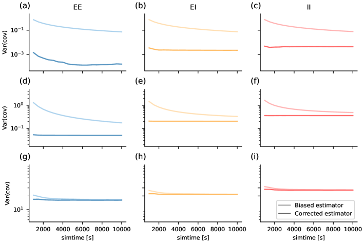
Figure A6: Bias correction of variance of covariance estimation for different simulation lengths at three different spectral radii $r$. The light color depicts the biased estimator, the dark color the corrected estimator Eq. (48). (a, b, c) $r=0.10$; (d, e, f) $r=0.49$; (g, h, i) $r=0.90$.

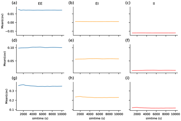
Figure A7: Mean of covariance estimation for different simulation lengths at three different spectral radii $r$. (a, b, c) $r=0.10$; (d, e, f) $r=0.49$; (g, h, i) $r=0.90$.

We utilize Eq. (4) in the supplementary information of Dahmen et al. [7] to correct for the bias in the estimation of the variances of covariances due to the finite simulation time. The analogous correction for two populations $a,b$ is given by

$$\delta C_{ab}^{2}=\delta\hat{C}_{ab}^{2}-\frac{\left\langle A_{a}\right\rangle\left\langle A_{b}\right\rangle-\left\langle C_{ab}\right\rangle^{2}}{N+1}\,,$$ (48)

with the biased estimator of the variance of cross-covariances $\delta\hat{C}_{ab}^{2}$, mean autocovariance $\left\langle A_{a}\right\rangle$, mean cross-covariance $\left\langle C_{ab}\right\rangle$, and the number of bins the spike trains are divided into $N=T_{\mathrm{sim}}/T_{\mathrm{bin}}$. Fig. A6 illustrates that after a simulation time of $10000\,\mathrm{s}$, the corrected estimator converges to a fixed value while the biased estimator does not, especially for smaller spectral radii. In contrast, the mean covariance estimator converges much faster for all spectral radii, as shown in Fig. A7.

L Numerical implementation of CVs

For computing the theoretical prediction of the CVs, we make use the equation found in Appendix A.1 in Brunel [42], which in our units reads

$$\mathrm{CV}^{2} = 2\pi\left(\tau_{\mathrm{m}}\nu\right)^{2}\int_{y_{\mathrm{r}}}^{y_{\mathrm{th}}}\mathrm{d}x\,\mathrm{e}^{x^{2}}\int_{-\infty}^{x}\mathrm{d}s\,\mathrm{e}^{s^{2}}\left[1+\mathrm{erf}\left(s\right)\right]^{2}\,.$$ (49)

However, a naive implementation of Eq. (49) is numerically unstable due to the diverging integrals. To proceed, we rewrite Eq. (49) using the following steps:

$$\mathrm{CV}^{2} =2\pi\left(\tau_{\mathrm{m}}\nu\right)^{2}\int_{y_{\mathrm{r}}}^{y_{\mathrm{th}}}\mathrm{d}x\,\mathrm{e}^{x^{2}}\int_{-\infty}^{x}\mathrm{d}s\,\mathrm{e}^{s^{2}}\left(1+\mathrm{erf}\left(s\right)\right)^{2}$$

$$=2\pi\left(\tau_{\mathrm{m}}\nu\right)^{2}\int_{y_{\mathrm{r}}}^{y_{\mathrm{th}}}\mathrm{d}x\,\mathrm{e}^{x^{2}}\int_{-\infty}^{x}\mathrm{d}s\,\mathrm{e}^{s^{2}}\left(\frac{2}{\sqrt{\pi}}\int_{-\infty}^{s}\mathrm{e}^{-w^{2}}\mathrm{d}w\right)^{2}$$

$$=8\left(\tau_{\mathrm{m}}\nu\right)^{2}\int_{y_{\mathrm{r}}}^{y_{\mathrm{th}}}\mathrm{d}x\int_{-\infty}^{x}\mathrm{d}s\int_{-\infty}^{s}\mathrm{d}v\int_{-\infty}^{s}\mathrm{d}w\,\mathrm{e}^{x^{2}+s^{2}-v^{2}-w^{2}}\,.$$

We make a change of variables $v^{\prime}=s-v$, $w^{\prime}=s-w$, where we immediately drop the prime, yielding

$$\mathrm{CV}^{2} = 8\left(\tau_{\mathrm{m}}\nu\right)^{2}\int_{y_{\mathrm{r}}}^{y_{\mathrm{th}}}\mathrm{d}x\int_{0}^{\infty}\mathrm{d}v\int_{0}^{\infty}\mathrm{d}w\int_{-\infty}^{x}\mathrm{d}s\,\mathrm{e}^{x^{2}-s^{2}-v^{2}-w^{2}+2\left(v+w\right)s}\,.$$

Another change of variables $s^{\prime}=x+v+w-s$ gives

$$\mathrm{CV}^{2} = 8\left(\tau_{\mathrm{m}}\nu\right)^{2}\int_{y_{\mathrm{r}}}^{y_{\mathrm{th}}}\mathrm{d}x\int_{0}^{\infty}\mathrm{d}v\int_{0}^{\infty}\mathrm{d}w\int_{v+w}^{\infty}\mathrm{d}s\,\mathrm{e}^{-s^{2}+2vw+2sx}\,.$$

We switch the order of integration using $\int_{0}^{\infty}\mathrm{d}v\int_{0}^{\infty}\mathrm{d}w\int_{v+w}^{\infty}\mathrm{d}s=\int_{0}^{\infty}\mathrm{d}s\int_{0}^{s}\mathrm{d}v\int_{0}^{s-v}\mathrm{d}w$, which yields the form we used for the numerical implementation

$$\mathrm{CV}^{2} =8\left(\tau_{\mathrm{m}}\nu\right)^{2}\int_{0}^{\infty}\mathrm{d}s\int_{0}^{s}\mathrm{d}v\int_{0}^{s-v}\mathrm{d}w\int_{y_{\mathrm{r}}}^{y_{\mathrm{th}}}\mathrm{d}x\,\mathrm{e}^{-s^{2}+2vw+2sx}$$

$$=8\left(\tau_{\mathrm{m}}\nu\right)^{2}\int_{0}^{\infty}\mathrm{d}s\int_{0}^{s}\mathrm{d}v\,\mathrm{e}^{-s^{2}}\int_{0}^{s-v}\mathrm{d}w\,\mathrm{e}^{2vw}\int_{y_{\mathrm{r}}}^{y_{\mathrm{th}}}\mathrm{d}x\,\mathrm{e}^{2sx}$$

$$=2\left(\tau_{\mathrm{m}}\nu\right)^{2}\int_{0}^{\infty}\mathrm{d}s\int_{0}^{s}\mathrm{d}v\,\mathrm{e}^{-s^{2}}\frac{1}{v}\left[\mathrm{e}^{2v\left(s-v\right)}-1\right]\frac{1}{s}\left[\mathrm{e}^{2sy_{\mathrm{th}}}-\mathrm{e}^{2sy_{\mathrm{r}}}\right]$$

$$=2\left(\tau_{\mathrm{m}}\nu\right)^{2}\int_{0}^{\infty}\mathrm{d}s\,\frac{1}{s}\left[\mathrm{e}^{2sy_{\mathrm{th}}}-\mathrm{e}^{2sy_{\mathrm{r}}}\right]\int_{0}^{s}\mathrm{d}v\,\frac{1}{v}\left[\mathrm{e}^{-s^{2}-2v^{2}+2sv}-\mathrm{e}^{-s^{2}}\right]\,.$$

References

- Griffith and Horn [1966] J. S. Griffith and G. Horn, An analysis of spontaneous impulse activity of units in the striate cortex of unrestrained cats, J. Physiol. 186, 516 (1966).
- Koch and Fuster [1989] K. W. Koch and J. M. Fuster, Unit activity in monkey parietal cortex related to haptic perception and temporary memory, Exp. Brain Res. 76, 292 (1989).
- Dąbrowska et al. [2021] P. A. Dąbrowska, N. Voges, M. von Papen, J. Ito, D. Dahmen, A. Riehle, T. Brochier, and S. Grün, On the Complexity of Resting State Spiking Activity in Monkey Motor Cortex, Cereb. Cortex Commun. 2 (2021), 10.1093/texcom/tgab033, tgab033.
- Shinomoto et al. [2003] S. Shinomoto, K. Shima, and J. Tanji, Differences in spiking patterns among cortical neurons, Neural Comput. 15, 2823 (2003).
- Ecker et al. [2010] A. S. Ecker, P. Berens, G. A. Keliris, M. Bethge, and N. K. Logothetis, Decorrelated neuronal firing in cortical microcircuits, Science 327, 584 (2010).
- Cohen and Kohn [2011] M. R. Cohen and A. Kohn, Measuring and interpreting neuronal correlations, Nat. Rev. Neurosci. 14, 811 (2011).
- Dahmen et al. [2019] D. Dahmen, S. Grün, M. Diesmann, and M. Helias, Second type of criticality in the brain uncovers rich multiple-neuron dynamics, Proc. Natl. Acad. Sci. USA 116, 13051 (2019).
- Dahmen et al. [2022a] D. Dahmen, M. Layer, L. Deutz, P. A. Dąbrowska, N. Voges, M. von Papen, T. Brochier, A. Riehle, M. Diesmann, S. Grün, et al., Global organization of neuronal activity only requires unstructured local connectivity, eLife 11, e68422 (2022a).
- da Silveira and Berry [2013] R. A. da Silveira and M. J. Berry, High-fidelity coding with correlated neurons, ArXiv (2013).
- Moreno-Bote et al. [2014] R. Moreno-Bote, J. Beck, I. Kanitscheider, X. Pitkow, P. Latham, and A. Pouget, Information-limiting correlations, Nat. Neurosci. 17, 1410 (2014).
- Stringer et al. [2019] C. Stringer, M. Pachitariu, N. Steinmetz, M. Carandini, and K. D. Harris, High-dimensional geometry of population responses in visual cortex, Nature 571, 361 (2019).
- Vyas et al. [2020] S. Vyas, M. D. Golub, D. Sussillo, and K. V. Shenoy, Computation Through Neural Population Dynamics, Annu. Rev. Neurosci. 43, 249 (2020).
- Jun et al. [2017] J. J. Jun, N. A. Steinmetz, J. H. Siegle, D. J. Denman, M. Bauza, B. Barbarits, A. K. Lee, C. A. Anastassiou, A. Andrei, Ç. Aydın, M. Barbic, T. J. Blanche, V. Bonin, J. Couto, B. Dutta, S. L. Gratiy, D. A. Gutnisky, M. Häusser, B. Karsh, P. Ledochowitsch, C. M. Lopez, C. Mitelut, S. Musa, M. Okun, M. Pachitariu, J. Putzeys, P. D. Rich, C. Rossant, W.-l. Sun, K. Svoboda, M. Carandini, K. D. Harris, C. Koch, J. O’Keefe, and T. D. Harris, Fully integrated silicon probes for high-density recording of neural activity, Nature 551, 232 (2017).
- Steinmetz et al. [2021] N. A. Steinmetz, C. Aydin, A. Lebedeva, M. Okun, M. Pachitariu, M. Bauza, M. Beau, J. Bhagat, C. Böhm, M. Broux, S. Chen, J. Colonell, R. J. Gardner, B. Karsh, F. Kloosterman, D. Kostadinov, C. Mora-Lopez, J. O’Callaghan, J. Park, J. Putzeys, B. Sauerbrei, R. J. J. van Daal, A. Z. Vollan, S. Wang, M. Welkenhuysen, Z. Ye, J. T. Dudman, B. Dutta, A. W. Hantman, K. D. Harris, A. K. Lee, E. I. Moser, J. O’Keefe, A. Renart, K. Svoboda, M. Häusser, S. Haesler, M. Carandini, and T. D. Harris, Neuropixels 2.0: A miniaturized high-density probe for stable, long-term brain recordings, Science 372 (2021), 10.1126/science.abf4588.
- Campagnola et al. [2022] L. Campagnola, S. C. Seeman, T. Chartrand, L. Kim, A. Hoggarth, C. Gamlin, S. Ito, J. Trinh, P. Davoudian, C. Radaelli, et al., Local connectivity and synaptic dynamics in mouse and human neocortex, Science 375, eabj5861 (2022).
- Roxin et al. [2011] A. Roxin, N. Brunel, D. Hansel, G. Mongillo, and C. van Vreeswijk, On the distribution of firing rates in networks of cortical neurons, J. Neurosci. 31, 16217 (2011).
- White et al. [1986] J. G. White, E. Southgate, J. N. Thomson, and S. Brenner, The structure of the nervous system of the nematode caenorhabditis elegans, Philos. Trans. R. Soc. B 314, 1 (1986).
- Markov et al. [2014] N. T. Markov, M. M. Ercsey-Ravasz, A. R. Ribeiro Gomes, C. Lamy, L. Magrou, J. Vezoli, P. Misery, A. Falchier, R. Quilodran, M. A. Gariel, J. Sallet, R. Gamanut, C. Huissoud, S. Clavagnier, P. Giroud, D. Sappey-Marinier, P. Barone, C. Dehay, Z. Toroczkai, K. Knoblauch, D. C. Van Essen, and H. Kennedy, A weighted and directed interareal connectivity matrix for macaque cerebral cortex, Cereb. Cortex 24, 17 (2014).
- van Albada et al. [2022] S. J. van Albada, A. Morales-Gregorio, T. Dickscheid, A. Goulas, R. Bakker, S. Bludau, G. Palm, C.-C. Hilgetag, and M. Diesmann, Bringing anatomical information into neuronal network models, in Computational Modelling of the Brain: Modelling Approaches to Cells, Circuits and Networks, edited by M. Giugliano, M. Negrello, and D. Linaro (Springer International Publishing, Cham, 2022) pp. 201–234.
- Schnepel et al. [2015] P. Schnepel, A. Kumar, M. Zohar, A. Aertsen, and C. Boucsein, Physiology and impact of horizontal connections in rat neocortex, Cereb. Cortex 25, 3818 (2015).
- Sayer et al. [1990] R. Sayer, M. Friedlander, and S. Redman, The time course and amplitude of epsps evoked at synapses between pairs of ca3/ca1 neurons in the hippocampal slice, J. Neurosci. 10, 826 (1990).
- Feldmeyer et al. [1999] D. Feldmeyer, V. Egger, J. Lübke, and B. Sakmann, Reliable synaptic connections between pairs of excitatory layer 4 neurones within a single "barrel" of developing rat somatosensory cortex, J. Physiol. 521, 169 (1999).
- Song et al. [2005] S. Song, P. Sjöström, M. Reigl, S. Nelson, and D. Chklovskii, Highly nonrandom features of synaptic connectivity in local cortical circuits, PLOS Biol. 3, e68 (2005).
- Lefort et al. [2009] S. Lefort, C. Tomm, J.-C. F. Sarria, and C. C. H. Petersen, The excitatory neuronal network of the C2 barrel column in mouse primary somatosensory cortex, Neuron 61, 301 (2009).
- Ikegaya et al. [2013] Y. Ikegaya, T. Sasaki, D. Ishikawa, N. Honma, K. Tao, N. Takahashi, G. Minamisawa, S. Ujita, and N. Matsuki, Interpyramid spike transmission stabilizes the sparseness of recurrent network activity, Cereb. Cortex 23, 293 (2013).
- Loewenstein et al. [2011] Y. Loewenstein, A. Kuras, and S. Rumpel, Multiplicative dynamics underlie the emergence of the log-normal distribution of spine sizes in the neocortex in vivo, J. Neurosci. 31, 9481 (2011).
- Lindner et al. [2005] B. Lindner, B. Doiron, and A. Longtin, Theory of oscillatory firing induced by spatially correlated noise and delayed inhibitory feedback, Phys. Rev. E 72, 061919 (2005).
- Pernice et al. [2011] V. Pernice, B. Staude, S. Cardanobile, and S. Rotter, How structure determines correlations in neuronal networks, PLOS Comput. Biol. 7, e1002059 (2011).
- Pernice et al. [2012] V. Pernice, B. Staude, S. Cardanobile, and S. Rotter, Recurrent interactions in spiking networks with arbitrary topology, Phys. Rev. E 85, 031916 (2012).
- Trousdale et al. [2012] J. Trousdale, Y. Hu, E. Shea-Brown, and K. Josic, Impact of network structure and cellular response on spike time correlations. PLOS Comput. Biol. 8, e1002408 (2012).
- Grytskyy et al. [2013] D. Grytskyy, T. Tetzlaff, M. Diesmann, and M. Helias, A unified view on weakly correlated recurrent networks, Front. Comput. Neurosci. 7, 131 (2013).
- Dahmen et al. [2016] D. Dahmen, H. Bos, and M. Helias, Correlated fluctuations in strongly coupled binary networks beyond equilibrium, Phys. Rev. X 6, 031024 (2016).
- Ginzburg and Sompolinsky [1994] I. Ginzburg and H. Sompolinsky, Theory of correlations in stochastic neural networks, Phys. Rev. E 50, 3171 (1994).
- van Vreeswijk and Sompolinsky [1996] C. van Vreeswijk and H. Sompolinsky, Chaos in neuronal networks with balanced excitatory and inhibitory activity, Science 274, 1724 (1996).
- Buice et al. [2010] M. A. Buice, J. D. Cowan, and C. C. Chow, Systematic fluctuation expansion for neural network activity equations, Neural Comput. 22, 377 (2010).
- Renart et al. [2010] A. Renart, J. De La Rocha, P. Bartho, L. Hollender, N. Parga, A. Reyes, and K. D. Harris, The asynchronous state in cortical circuits, Science 327, 587 (2010).
- Tetzlaff et al. [2012] T. Tetzlaff, M. Helias, G. T. Einevoll, and M. Diesmann, Decorrelation of neural-network activity by inhibitory feedback, PLOS Comput. Biol. 8, e1002596 (2012).
- Montbrió et al. [2015] E. Montbrió, D. Pazó, and A. Roxin, Macroscopic description for networks of spiking neurons, Phys. Rev. X 5, 021028 (2015).
- Sompolinsky and Zippelius [1982] H. Sompolinsky and A. Zippelius, Relaxational dynamics of the edwards-anderson model and the mean-field theory of spin-glasses, Phys. Rev. B 25, 6860 (1982).
- Helias and Dahmen [2020] M. Helias and D. Dahmen, Statistical Field Theory for Neural Networks (Springer International Publishing, 2020) p. 203.
- Dahmen et al. [2022b] D. Dahmen, S. Recanatesi, X. Jia, G. K. Ocker, L. Campagnola, T. Jarsky, S. Seeman, M. Helias, and E. Shea-Brown, Strong and localized recurrence controls dimensionality of neural activity across brain areas, BioRxiv (2022b).
- Brunel [2000] N. Brunel, Dynamics of sparsely connected networks of excitatory and inhibitory spiking neurons, J. Comput. Neurosci. 8, 183 (2000).
- Stein [1967] R. B. Stein, Some models of neuronal variability, Biomed. Pharmacol. J. 7, 37 (1967).
- Tuckwell [1988] H. C. Tuckwell, Introduction to Theoretical Neurobiology, Vol. 1 (Cambridge University Press, Cambridge, 1988).
- Brunel and Hakim [1999] N. Brunel and V. Hakim, Fast global oscillations in networks of integrate-and-fire neurons with low firing rates, Neural Comput. 11, 1621 (1999).
- Siegert [1951] A. J. Siegert, On the first passage time probability problem, Phys. Rev. 81, 617 (1951).
- Helias et al. [2013] M. Helias, T. Tetzlaff, and M. Diesmann, Echoes in correlated neural systems, New. J. Phys. 15, 023002 (2013).
- Tetzlaff et al. [2007] T. Tetzlaff, S. Rotter, E. Stark, M. Abeles, A. Aertsen, and M. Diesmann, Dependence of neuronal correlations on filter characteristics and marginal spike-train statistics, (2007), in press.
- Shea-Brown et al. [2008] E. Shea-Brown, K. c. v. Josić, J. de la Rocha, and B. Doiron, Correlation and synchrony transfer in integrate-and-fire neurons: Basic properties and consequences for coding, Phys. Rev. Lett. 100, 108102 (2008).
- Cox and Lewis [1966] D. R. Cox and P. A. W. Lewis, The Statistical Analysis of Series of Events, Methuen’s Monographs on Applied Probability and Statistics (Methuen, London, 1966).
- Layer et al. [2022] M. Layer, J. Senk, S. Essink, A. van Meegen, H. Bos, and M. Helias, NNMT: Mean-field based analysis tools for neuronal network models, Front. Neuroinform. 16, 835657 (2022).
- Fischer and Hertz [1991] K. Fischer and J. Hertz, Spin glasses (Cambridge University Press, 1991).
- Hertz et al. [2017] J. A. Hertz, Y. Roudi, and P. Sollich, Path integral methods for the dynamics of stochastic and disordered systems, J. Phys. A 50, 033001 (2017).
- Sompolinsky et al. [1988] H. Sompolinsky, A. Crisanti, and H. J. Sommers, Chaos in random neural networks, Phys. Rev. Lett. 61, 259 (1988).
- Sommers et al. [1988] H. Sommers, A. Crisanti, H. Sompolinsky, and Y. Stein, Spectrum of large random asymmetric matrices, Phys. Rev. Lett. 60, 1895 (1988).
- De Dominicis [1978] C. De Dominicis, Dynamics as a substitute for replicas in systems with quenched random impurities, Phys. Rev. B 18, 4913 (1978).
- van Vreeswijk and Sompolinsky [1998] C. van Vreeswijk and H. Sompolinsky, Chaotic balanced state in a model of cortical circuits, Neural Comput. 10, 1321 (1998).
- Zinn-Justin [1996] J. Zinn-Justin, Quantum field theory and critical phenomena (Clarendon Press, Oxford, 1996).
- Helias et al. [2014] M. Helias, T. Tetzlaff, and M. Diesmann, The correlation structure of local cortical networks intrinsically results from recurrent dynamics, PLOS Comput. Biol. 10, e1003428 (2014).
- Rosenbaum and Doiron [2014] R. Rosenbaum and B. Doiron, Balanced networks of spiking neurons with spatially dependent recurrent connections, Phys. Rev. X 4, 021039 (2014).
- Pyle and Rosenbaum [2017a] R. Pyle and R. Rosenbaum, Spatiotemporal dynamics and reliable computations in recurrent spiking neural networks, Phys. Rev. Lett. 118, 018103 (2017a).
- Pyle and Rosenbaum [2017b] R. Pyle and R. Rosenbaum, Spatiotemporal dynamics and reliable computations in recurrent spiking neural networks, Phys. Rev. Lett. 118 (2017b), 10.1103/physrevlett.118.018103.
- Darshan et al. [2018] R. Darshan, C. van Vreeswijk, and D. Hansel, Strength of correlations in strongly recurrent neuronal networks, Phys. Rev. X 8, 031072 (2018).
- Smith et al. [2018] G. B. Smith, B. Hein, D. E. Whitney, D. Fitzpatrick, and M. Kaschube, Distributed network interactions and their emergence in developing neocortex, Nat. Neurosci. 21, 1600 (2018).
- Huang et al. [2019] C. Huang, D. A. Ruff, R. Pyle, R. Rosenbaum, M. R. Cohen, and B. Doiron, Circuit models of low-dimensional shared variability in cortical networks, Neuron 101, 337 (2019).
- Mastrogiuseppe and Ostojic [2018] F. Mastrogiuseppe and S. Ostojic, Linking connectivity, dynamics, and computations in low-rank recurrent neural networks, Neuron 99, 609 (2018).
- Kriener et al. [2014a] B. Kriener, M. Helias, S. Rotter, M. Diesmann, and G. T. Einevoll, How pattern formation in ring networks of excitatory and inhibitory spiking neurons depends on the input current regime, Front. Comput. Neurosci. 7, 1 (2014a).
- Aljadeff et al. [2016] J. Aljadeff, D. Renfrew, M. Vegué, and T. O. Sharpee, Low-dimensional dynamics of structured random networks, Phys. Rev. E 93, 022302 (2016).
- Rajan and Abbott [2006] K. Rajan and L. F. Abbott, Eigenvalue spectra of random matrices for neural networks, Phys. Rev. Lett. 97, 188104 (2006).
- Ostojic [2014] S. Ostojic, Two types of asynchronous activity in networks of excitatory and inhibitory spiking neurons, Nat. Neurosci. 17, 594 (2014).
- Amit and Brunel [1997] D. J. Amit and N. Brunel, Model of global spontaneous activity and local structured activity during delay periods in the cerebral cortex, Cereb. Cortex 7, 237 (1997).
- Kriener et al. [2014b] B. Kriener, H. Enger, T. Tetzlaff, H. E. Plesser, M.-O. Gewaltig, and G. T. Einevoll, Dynamics of self-sustained asynchronous-irregular activity in random networks of spiking neurons with strong synapses. Front. Comput. Neurosci. 8, 136 (2014b).
- Stern et al. [2014] M. Stern, H. Sompolinsky, and L. F. Abbott, Dynamics of random neural networks with bistable units, Phys. Rev. E 90, 062710 (2014).
- Aljadeff et al. [2015] J. Aljadeff, M. Stern, and T. Sharpee, Transition to chaos in random networks with cell-type-specific connectivity, Phys. Rev. Lett. 114, 088101 (2015).
- Martí et al. [2018] D. Martí, N. Brunel, and S. Ostojic, Correlations between synapses in pairs of neurons slow down dynamics in randomly connected neural networks, Phys. Rev. E 97, 062314 (2018).
- Schuecker et al. [2018] J. Schuecker, S. Goedeke, and M. Helias, Optimal sequence memory in driven random networks, Phys. Rev. X 8, 041029 (2018).
- Crisanti and Sompolinsky [2018] A. Crisanti and H. Sompolinsky, Path integral approach to random neural networks, Phys. Rev. E 98, 062120 (2018).
- Muscinelli et al. [2019] S. P. Muscinelli, W. Gerstner, and T. Schwalger, How single neuron properties shape chaotic dynamics and signal transmission in random neural networks, PLOS Comput. Biol. 15, e1007122 (2019).
- Beiran and Ostojic [2019] M. Beiran and S. Ostojic, Contrasting the effects of adaptation and synaptic filtering on the timescales of dynamics in recurrent networks, PLOS Comput. Biol. 15, e1006893 (2019).
- Kuśmierz et al. [2020] L. Kuśmierz, S. Ogawa, and T. Toyoizumi, Edge of chaos and avalanches in neural networks with heavy-tailed synaptic weight distribution, Phys. Rev. Lett. 125, 028101 (2020).
- Wardak and Gong [2022] A. Wardak and P. Gong, Extended anderson criticality in heavy-tailed neural networks, Phys. Rev. Lett. 129, 048103 (2022).
- Rosenbaum et al. [2017] R. Rosenbaum, M. A. Smith, A. Kohn, J. E. Rubin, and B. Doiron, The spatial structure of correlated neuronal variability, Nat. Neurosci. 20, 107 (2017).
- Baker et al. [2019] C. Baker, C. Ebsch, I. Lampl, and R. Rosenbaum, Correlated states in balanced neuronal networks, Phys. Rev. E 99, 052414 (2019).
- Litwin-Kumar and Doiron [2012] A. Litwin-Kumar and B. Doiron, Slow dynamics and high variability in balanced cortical networks with clustered connections, Nat. Neurosci. 15, 1498 (2012).
- Brinkman et al. [2022] B. A. Brinkman, H. Yan, A. Maffei, I. M. Park, A. Fontanini, J. Wang, and G. La Camera, Metastable dynamics of neural circuits and networks, Applied Physics Reviews 9 (2022).
- Bressloff [2012] P. C. Bressloff, Spatiotemporal dynamics of continuum neural fields, J. Phys. A Math. Theor. 45, 033001 (2012).
- Zeraati et al. [2023] R. Zeraati, Y.-L. Shi, N. A. Steinmetz, M. A. Gieselmann, A. Thiele, T. Moore, A. Levina, and T. A. Engel, Intrinsic timescales in the visual cortex change with selective attention and reflect spatial connectivity, Nat. Commun. 14, 1858 (2023).
- Shi et al. [2023] Y.-L. Shi, R. Zeraati, A. Levina, and T. A. Engel, Spatial and temporal correlations in neural networks with structured connectivity, Phys. Rev. Res. 5, 013005 (2023).
- Gewaltig and Diesmann [2007] M.-O. Gewaltig and M. Diesmann, NEST (NEural Simulation Tool), Scholarpedia J. 2, 1430 (2007).
- Gardiner [1985] C. W. Gardiner, Handbook of Stochastic Methods for Physics, Chemistry and the Natural Sciences, 2nd ed., Springer Series in Synergetics No. 13 (Springer-Verlag, Berlin, 1985).
- Khintchine [1934] A. Khintchine, Korrelationstheorie der stationaeren stochastischen prozesse, Math. Ann. , 604 (1934).