Gravitational wave effects and phenomenology of a two-component dark matter model

Abstract

We study an extension of the Standard Model (SM) which could have two candidates for dark matter (DM) including a Dirac fermion and a Vector Dark Matter (VDM) under new $U(1)$ gauge group in the hidden sector. The model is classically scale invariant and the electroweak symmetry breaks because of the loop effects. We investigate the parameter space allowed by current experimental constraints and phenomenological bounds. We probe the parameter space of the model in the mass range $1<M_{V}<5000$ GeV and $1<M_{\psi}<5000$ GeV. It has been shown that there are many points in this mass range that are in agreement with all phenomenological constraints. The electroweak phase transition have been discussed and shown that there is region in the parameter space of the model consistent with DM relic density and direct detection constraints, while at the same time can lead to first order electroweak phase transition. The gravitational waves produced during the phase transition could be probed by future space-based interferometers such as LISA and BBO.

1 Introduction

The Standard Model (SM) has been the most effective way to describe the functioning of the world around us, but that is incomplete because of challenges like matter-antimatter asymmetry, hierarchy problem, and DM. DM is estimated to make up approximately 27 percent of our universe, as indicated by a lot of astrophysical and cosmological evidence[1]. One of the main goals of particle physicists is to predict and find a particle that can satisfy the properties of DM, which can be a window to physics beyond the standard model (BSM).

Weakly interacting massive particles (WIMPs) are the most popular candidate for DM, with the Freeze-out scenario being the most popular choice[2]. WIMP paradigm is essential background for almost any discussion of particle DM and the triple coincidence of motivations from particle theory, particle experiment, and cosmology is known as the WIMP miracle. However, no trace of DM has so far been found in direct detection experiments. Due to the strong constraints on direct detection experiments in one-component DM models, multi-component DM models seem more appropriate in some ways [3, 4, 5, 6, 7, 8, 9, 10, 11, 12, 13, 14, 15, 16, 17, 18, 19, 20, 21, 22, 23, 24, 25, 26, 27, 28, 29, 30, 31, 32, 33, 34, 35, 36, 37, 38, 39, 40, 41, 42, 43, 44, 45, 46, 47, 48, 49, 50, 51, 52].

In the SM, electroweak phase transition is of second order[53, 54] and does not generate the gravitational wave (GW) signal (for a recent review see [55]). A first-order phase transition can be caused by certain extensions of the SM and the DM candidate, leading to the creation of GWs[56, 57, 58, 59, 60, 61, 62, 63, 64, 65, 66, 67, 68, 69, 70, 71, 72, 73, 74, 75, 76, 77, 78, 79, 80, 81, 82, 83, 84]. In the early Universe when two local minima of free energy (potential) co-exist for some range of temperatures (critical temperature), strongly first order electroweak phase transition can take place. After that, the relevant scalar field can quantum mechanically tunnel into the new phase and through the nucleation of bubbles and collide with each other to cause a significant background of GWs[85, 86, 87, 88, 89].The discovery of GWs resulting from the first-order phase transition can be the consequence of physics BSM, which can be a supplement to ground experiments like LHC. Unlike GWs from strong astrophysical sources[90], these waves have a range between milli-hertz and deci-hertz[91]. The Laser Interferometer Space Antenna (LISA)[92] and Big Bang Observer (BBO)[93] are two space-based GWs detectors which are expected to observe GWs resulting from cosmological phase transitions in future years. On the other hand, one of the Sakharov conditions[94] that explains the matter-antimatter asymmetry in universe is the thermal imbalance that occurs in first-order phase transitions.

As mentioned, one of the fundamental challenges of particle physics is the hierarchy problem. A potential solution to this problem is to drop the Higgs mass term in the potential. SM without the Higgs mass term is scale invariant. In this paper, we present a classically scale-invariant extension of the SM where all the particle masses are generated using the Coleman-Weinberg mechanism[95]. The model includes three new fields, a fermion, a complex singlet scalar and a vector field with $U_{D}(1)$ gauge symmetry. We examine two scenarios in this paper. In scenario A, we consider only the fermionic field as DM. In scenario B, both fermionic and vector fields are considered as DM. We probe the parameter space of the model according to constraints from relic density and direct detection. DM relic density is reported by Planck Collaboration[96] and DM-Nucleon cross section is constrained by XENONnT experiment results[97]. We investigate the possibility of the electroweak phase transition with respect to the bounded parameter space, where we use the effects of the effective potential of the finite temperature. We probe parameter space of the model which is consistent with the said phenomenological constraints and also lead to a strong first-order electroweak phase transition. Also the GW signal resulting from this phase transition have been studied in the LISA and BBO detectors.

Here is the organization of the paper. In the next section, we introduce the model. In section. 3, we study the phenomenology of the Scenario A including relic density, direct detection, invisible Higgs decay and the resulting GWs. Section. 4 is dedicated to the phenomenology of the Scenario B and its GWs signals. Finally, our conclusion comes in section. 5.

2 The Model

In this section, we consider an extension of the SM to explain DM phenomenology. In this regards, the model contains three new fields in which a vector dark matter $V_{\mu}$ and a Dirac fermion field $\psi$ can play role of DM. Also a complex scalar S mediates between SM and dark sector. In the model $V_{\mu}$, $\psi$ and S are charged under a new dark $U(1)_{D}$ gauge group. All of these fields are singlet under SM gauge groups. We suppose mass of fermion was produced by breaking of dark $U_{D}(1)$ gauge symmetry and so was constrained by other parameters of the model. However, in the model, the dark sector is invariant under the transformations of $U_{D}(1)$ gauge group:

$$\psi_{L}\rightarrow e^{iQ_{l}\alpha(x)}\psi_{L},$$

$$\psi_{R}\rightarrow e^{iQ_{r}\alpha(x)}\psi_{R},$$

$$S\rightarrow e^{iQ_{s}\alpha(x)}S,$$

$$V_{\mu}\rightarrow V_{\mu}-\frac{1}{g_{v}}\partial_{\mu}{\alpha(x)}.$$ (2.1)

where the $U(1)_{D}$ charge of the new particles, $Q_{l,r,s}$, are given in Table 1.

The Lagrangian for the model is given by the following renormalizable interactions,

$${\cal L}={\cal L}_{SM}+i\bar{\psi}_{L}\gamma^{\mu}D_{\mu}\psi_{L}+i\bar{\psi}_{R}\gamma^{\mu}D_{\mu}\psi_{R}-g_{s}\bar{\psi}_{L}\psi_{R}S+h.c.-\frac{1}{4}V_{\mu\nu}V^{\mu\nu}+(D_{\mu}S)^{*}(D^{\mu}S)-V(H,S).$$ (2.2)

where ${\cal L}_{SM}$ is the SM Lagrangian without the Higgs potential term, The covariant derivative is

$$D_{\mu}=(\partial_{\mu}+iQg_{v}V_{\mu}),\quad\text{and}$$

$$V_{\mu\nu}=\partial_{\mu}V_{\nu}-\partial_{\nu}V_{\mu},$$ (2.3)

On the imposition of dark charge conjugation symmetry, we do not assume a kinetic mixing term between $V_{\mu}$ and the $U(1)_{Y}$ gauge boson of the SM.

Field	$S$	$\psi_{L}$	$\psi_{R}$
$U(1)_{D}$ charge	1	$\frac{1}{2}$	$-\frac{1}{2}$

Table 1: The charges of the dark sector particles under the new $U(1)_{D}$ symmetry.

The most general scale-invariant potential $V(H,S)$ which is renormalizable and invariant under gauge symmetry is

$$V(H,S)=\frac{1}{6}\lambda_{H}(H^{\dagger}H)^{2}+\frac{1}{6}\lambda_{S}(S^{*}S)^{2}+2\lambda_{SH}(S^{*}S)(H^{\dagger}H).$$ (2.4)

Note that the quartic portal interaction, $\lambda_{SH}(S^{*}S)(H^{\dagger}H)$, is the only connection between the dark sector and the SM.

SM Higgs field $H$ as well as dark scalar $S$ can receive VEVs breaking respectively the electroweak and $U_{D}(1)$ symmetries. In unitary gauge, the imaginary component of $S$ can be absorbed as the longitudinal part of $V_{\mu}$. In this gauge, we can write

$$H=\frac{1}{\sqrt{2}}\begin{pmatrix}0\\ h_{1}\end{pmatrix}\,\,\,and\,\,\,S=\frac{1}{\sqrt{2}}h_{2},$$ (2.5)

where $h_{1}$ and $h_{2}$ are real scalar fields which can get VEVs. Now, the tree-level potential becomes

$$V^{tree}=\frac{1}{4!}\lambda_{H}h_{1}^{4}+\frac{1}{4!}\lambda_{S}h_{2}^{4}+\frac{1}{2}\lambda_{SH}h_{1}^{2}h_{2}^{2}.$$ (2.6)

There is a $Z_{2}$ symmetry for $\psi$, making it a stable particle. In addition, if the mass of $V_{\mu}$ is less than two times of the mass of $\psi$, then both $V_{\mu}$ and $\psi$ are viable DM candidates.

For the Hessian matrix, we define:

$$H_{ij}(h_{1},h_{2})\equiv\frac{\partial^{2}V^{tree}}{\partial h_{i}\partial h_{j}}.$$ (2.7)

Necessary and sufficient conditions for local minimum of $V^{tree}$ in which vacuum expectation values $\langle h_{1}\rangle=\nu_{1}$ $\rm and$ $\langle h_{2}\rangle=\nu_{2}$, have be written as:

$$\frac{\partial V^{tree}}{\partial h_{i}}\bigg{\rvert}_{\nu_{1},\nu_{2}}=0$$ (2.8)

$$\frac{\partial^{2}V^{tree}}{\partial h_{i}^{2}}\bigg{\rvert}_{\nu_{1},\nu_{2}}>0$$ (2.9)

$$det(H(\nu_{1},\nu_{2}))>0,$$ (2.10)

where $det(H(\nu_{1},\nu_{2}))$ is determinant of the Hessian matrix. Condition (2.8) for non-vanishing VEVs leads to the following constraints

$$\lambda_{H}\lambda_{S}=(3!\lambda_{SH})^{2} \frac{\nu_{1}^{2}}{\nu_{2}^{2}}=-\frac{3!\lambda_{SH}}{\lambda_{H}}.$$ (2.11)

Conditions (2.8) and (2.9) require $\lambda_{H}>0$, $\lambda_{S}>0$, and $\lambda_{SH}<0$. However, condition (2.10) will not be satisfied, because $det(H(\nu_{1},\nu_{2}))=0$. When the determinant of the Hessian matrix is zero, the second derivative test is inconclusive, and the point $(\nu_{1},\nu_{2})$ could be any of a minimum, maximum or saddle point. However, in the model, constraint (2.11) defines as a flat direction, in which $V^{tree}=0$. Thus, it is the stationary line or a local minimum.

The important point is that for other directions $V_{eff}^{1-loop(T=0)}>0$, and the tree level potential only vanishes along the flat direction. Thus, the full potential of the theory will be dominated by higher-loop contributions along flat direction and specifically by the one-loop effective potential. Considering one-loop effective potential, $V_{eff}^{1-loop}$, can lead to a small curvature in the flat direction which picks out a specific value along the ray as the minimum with $V_{eff}^{1-loop}<0$ and vacuum expectation value $\nu^{2}=\nu_{1}^{2}+\nu_{2}^{2}$ characterized by a RG scale $\Lambda$. Since at the minimum of the one-loop effective potential $V^{tree}\geqslant 0$ and $V_{eff}^{1-loop}<0$, the minimum of $V_{eff}^{1-loop}$ along the flat direction (where $V^{tree}=0$) is a global minimum of the full potential, and so spontaneous symmetry breaking take places. As a result, we suppose $h_{1}\rightarrow\nu_{1}+h_{1}$ and $h_{2}\rightarrow\nu_{2}+h_{2}$ and the electroweak symmetry breaks with value $\nu_{1}=246$ GeV. In tree level potential since $h_{1}$ and $h_{2}$ mix with each other, they can be rewritten by the mass eigenstates $H_{1}$ and $H_{2}$ as

$$\begin{pmatrix}H_{1}\\ H_{2}\end{pmatrix}=\begin{pmatrix}cos\alpha~{}~{}~{}-sin\alpha\\ sin\alpha~{}~{}~{}~{}~{}cos\alpha\end{pmatrix}\begin{pmatrix}h_{1}\\ h_{2}\end{pmatrix},$$ (2.12)

where $H_{2}$ is along the flat direction, thus $M_{H_{2}}=0$, and $H_{1}$ is perpendicular to the flat direction which we identify it as the SM-like Higgs observed at the LHC with $M_{H_{1}}=125$ GeV. After the symmetry breaking, we have the following constraints:

$$\nu_{2}=\frac{M_{V}}{g_{v}}, sin\alpha=\frac{\nu_{1}}{\sqrt{\nu_{1}^{2}+\nu_{2}^{2}}}$$

$$M_{\psi}=\frac{g_{s}M_{V}}{\sqrt{2}g_{v}} \lambda_{H}=\frac{3M_{H_{1}}^{2}}{\nu_{1}^{2}}cos^{2}\alpha$$

$$\lambda_{S}=\frac{3M_{H_{1}}^{2}}{\nu_{2}^{2}}sin^{2}\alpha \lambda_{SH}=-\frac{M_{H_{1}}^{2}}{2\nu_{1}\nu_{2}}sin\alpha\,cos\alpha,$$

where $M_{\psi}$ and $M_{V}$ are the masses of vector and fermion fields after symmetry breaking. Conditions (LABEL:2-12) constrain free parameters of the model up to three independent parameters. We choose $M_{V}$, $M_{\psi}$ and $g_{v}$ as the independent parameters of the model.

Since in tree level, $M_{H_{2}}=0$, and the elastic scattering cross section of DM off nuclei becomes severely large, the model actually is excluded by direct detection experiments. However, the radiative corrections give a mass to the massless eigenstate $H_{2}$. The one-loop corrections to the potential, via the Gildener-Weinberg formalism [98], shift the scalon mass to the values that can be even higher than SM Higgs mass. Along the flat direction, the one-loop effective potential, has the general form [98]

$$V_{eff}^{1-loop(T=0)}=aH_{2}^{4}+bH_{2}^{4}\,\ln\frac{H_{2}^{2}}{\Lambda^{2}},$$ (2.14)

where $a$ and $b$ are the dimensionless constants that given by

$$a=\frac{1}{64\pi^{2}\nu^{4}}\sum_{k=1}^{n}g_{k}M_{k}^{4}\ln\frac{M_{k}^{2}}{\nu^{2}},$$

$$b=\frac{1}{64\pi^{2}\nu^{4}}\sum_{k=1}^{n}g_{k}M_{k}^{4}.$$ (2.15)

In (2.15), $M_{k}$ and $g_{k}$ are, the tree-level mass and the internal degrees of freedom of the particle $k$, respectively (In our convention $g_{k}$ takes positive values for bosons and negative ones for fermions).

Minimizing (2.14) shows that the potential has a non-trivial stationary point at a value of the RG scale $\Lambda$, given by

$$\Lambda=\nu\exp\left(\frac{a}{2b}+\frac{1}{4}\right),$$ (2.16)

Eq. (2.16) can now be used to find the form of the one-loop effective potential along the flat direction in terms of the one-loop VEV $\nu$

$$V_{eff}^{1-loop(T=0)}=bH_{2}^{4}\,\left(\ln\frac{H_{2}^{2}}{\nu^{2}}-\frac{1}{2}\right),$$ (2.17)

It is remarkable that the scalon does not remain massless beyond the tree approximation. Regarding $V_{eff}^{1-loop(T=0)}$, $M_{H_{2}}$ will be

$$M_{H_{2}}^{2}=\frac{d^{2}V_{eff}^{1-loop(T=0)}}{dH_{2}^{2}}\bigg{\rvert}_{\nu}=8b\nu^{2}.$$ (2.18)

Considering (2.15), the scalon mass can be expressed in terms of other particle masses

$$M_{H_{2}}^{2}=\frac{1}{8\pi^{2}\nu^{2}}\left(M_{H_{1}}^{4}+6M_{W}^{4}+3M_{Z}^{4}+3M_{V}^{4}-12M_{t}^{4}-4M_{\psi}^{4}\right).$$ (2.19)

where $M_{W,Z,t}$ are the masses of W, Z gauge bosons, and top quark, respectively. As it was mentioned before $M_{H_{1}}=125$ GeV and $\nu^{2}=\nu_{1}^{2}+\nu_{2}^{2}$. Notice that in order to $V_{eff}^{1-loop(T=0)}$ be a minimum, it must be less than the value of the potential at the origin, hence it must be negative. From (2.19), we have a constraint on the parameter space of our model where $M_{H_{2}}>0$.

Note that according to (2.19) and (LABEL:2-12), $M_{H_{2}}$ is completely determined by the independent parameters of the model, i.e., $M_{V}$, $M_{\psi}$ and the coupling $g_{v}$ . These constraints are due to the scale invariance conditions which were imposed to the model. Depending on the new particle masses of our model, we examine two different scenarios. In scenario A, $\psi$ field is considered as DM. In scenario B, $M_{V}<2M_{\psi}$ and both $V_{\mu}$ and $\psi$ fields are considered as DM. In the following, we examine the phenomenology of each scenario separately.

3 Scenario A

3.1 DM phenomenology

3.1.1 Relic density

In this case, since we do not assume $M_{V}<2M_{\psi}$, the only candidate for DM is $\psi$. In the WIMP scenario, first early Universe is hot and very dense and all particles are in thermal equilibrium. Then Universe cools until its temperature reaches below the mass of DM particles, the number of DM becomes Boltzmann suppressed, dropping exponentially as $e^{-m_{X}/T}$. As the universe expands, the DM particles are diluted and can no longer find each other until they are annihilated and are out of thermal equilibrium with the SM particles. Then the DM particles freeze out and their number asymptotically reaches a constant value as their thermal relic density. The evolution of the number density of DM particle $(n_{\psi})$ with time is governed by the Boltzmann equation:

$$\dot{n_{\psi}}+3Hn_{\psi}=-\langle\sigma_{ann}\nu_{rel}\rangle[n_{\psi}^{2}-(n_{\psi}^{eq})^{2}],$$ (3.1)

where $H$ is the Hubble parameter and $n_{\psi}^{eq}\sim(m_{\psi}T)^{3/2}e^{-m_{\psi}/T}$ is the particle density before particles get out of equilibrium. The relevant Feynman diagrams for DM production are shown in the Figure 1. We calculate the relic density numerically for the $\psi$ particle by implementing the model into micrOMEGAs [99]. Figure 2 shows the parameter space of the model in agreement with the observed density relic[96]. As can be seen, there is agreement for $700<M_{V}<5000$ GeV , $30<M_{\psi}<5000$ GeV and $0.1<g_{v}<6$.

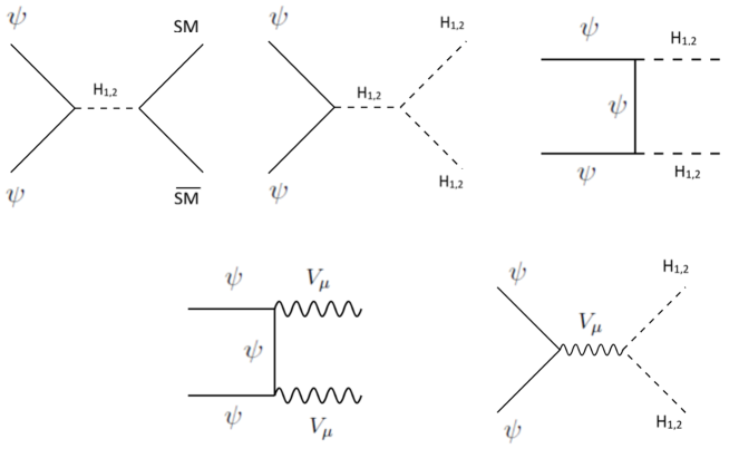
Figure 1: The relevant Feynman diagrams for DM relic density production cross section.

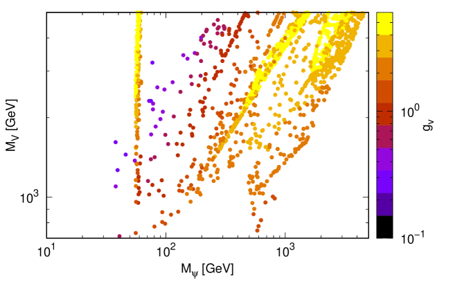
Figure 2: The allowed range of parameter space consistent with DM relic density.

3.1.2 Direct detection

WIMPs may be detected by its scattering off normal matter through processes $XSM$ → $XSM$. Given a typical WIMP mass of $m_{X}\sim 100$ GeV and WIMP velocity $\upsilon\sim 10^{-3}$, the deposited recoil energy is limited to $\sim 100$ keV, so it requires highly-sensitive, low-background and deep-site detectors. Such detectors are insensitive to very strongly-interacting DM, which would be stopped in the atmosphere or earth and would be undetectable underground. The spin-independent direct detection(DD) cross sections of ${\psi}$ was obtained using the micrOMEGAs package [99].

In figure 3, the parameter space of the model is drawn in agreement with the limits of relic density, XENONnT and neutrino floor. For $30<M_{\psi}<4000$ GeV, there will be points of the parameter space that fall below the XENONnT limit. As can be seen from Figure 3, for $M_{\psi}<M_{H_{1}}/2$ there will be points that allow the investigation of the invisibility Higgs decay, which will be investigated in the next section.

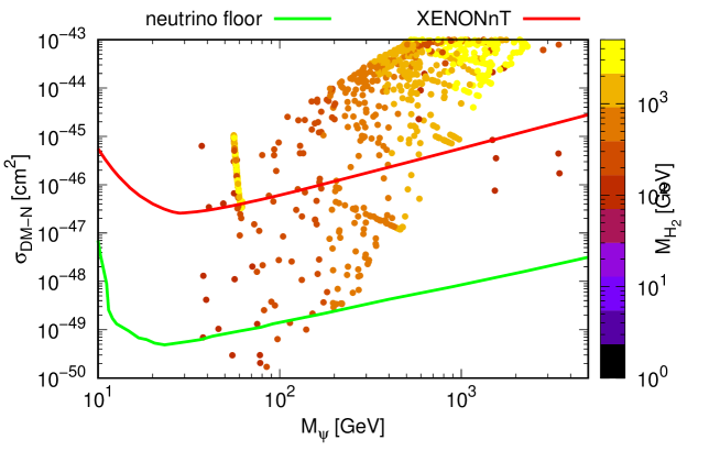
Figure 3: The allowed range of parameter space consistent with DM relic density and DD.

3.1.3 Invisible Higgs decay

As mentioned for parameters space consistent with $\psi$ relic density and DD, SM Higgs($H_{1}$) can only kinematically decay into a pair of ${\psi}$. Therefore, $H_{1}$ can contribute to the invisible decay mode with a branching ratio:

$$Br(H_{1}\rightarrow\rm Invisible) =\frac{\Gamma(H_{1}\rightarrow{\psi}{\psi})}{\Gamma(h)_{SM}+\Gamma(H_{1}\rightarrow{\psi}{\psi})},$$ (3.2)

where $\Gamma(h)_{SM}=4.15~{}\rm[MeV]$ is total width of Higgs boson[100]. The partial width for process $H_{1}\rightarrow{\psi}{\psi}$ is given by:

$$\Gamma(H_{1}\rightarrow{\psi}{\psi}) =\frac{M_{H_{1}}g_{s}^{2}sin^{2}\theta}{8\pi}(1-\frac{4M_{{\psi}}^{2}}{{M_{H_{1}}^{2}}})^{3/2}.$$ (3.3)

The SM prediction for the branching ratio of the Higgs boson decaying to invisible particles which coming from process $h\rightarrow ZZ^{*}\rightarrow 4\nu$ [101],[102],[103],[104] is, $1.2\times 10^{-3}.$ CMS Collaboration has reported the observed (expected) upper limit on the invisible branching fraction of the Higgs boson to be $0.18(0.10)$ at the $95\%$ confidence level, by assuming the SM production cross section [105]. A Similar analysis was performed by ATLAS collaboration in which an observed upper limit of $0.145$ is placed on the branching fraction of its decay into invisible particles at a $95\%$ confidence level[106].

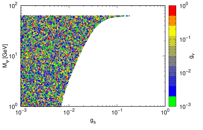
Figure 4: The cross points depict allowed region which is consistent with invisible Higgs decay at [106].

Figure 4, shows the allowed range of parameters by considering ATLAS [106] upper limit for invisible Higgs mode.

3.2 Electroweak phase transition and gravitational waves

3.2.1 Finite temperature potential

In addition to the 1-loop zero-temperature potential (2.17), we can also consider the 1-loop corrections at finite temperature in the effective potential, which is as follows[107]

$$V_{eff}^{1-loop(T\neq 0)}(H_{2},T)=\frac{T^{4}}{2\pi^{2}}\sum_{k=1}^{n}g_{k}J_{B,F}\Bigl{(}\frac{M_{k}}{\nu}\frac{H_{2}}{T}\Bigl{)},$$ (3.4)

with thermal functions

$$J_{B,F}(x)=\int_{0}^{\infty}dyy^{2}ln\Bigl{(}1\mp e^{-\sqrt{y^{2}+x^{2}}}\Bigl{)}.$$ (3.5)

The above functions can be expanded in terms of modified Bessel functions of the second kind, $K_{2}(x)$[70],

$$J_{B}(x)\simeq-\sum_{k=1}^{3}\frac{1}{k^{2}}x^{2}K_{2}(kx),$$

$$J_{F}(x)\simeq-\sum_{k=1}^{2}\frac{(-1)^{k}}{k^{2}}x^{2}K_{2}(kx).$$

The contribution of resummed daisy graphs is also as follows[108]

$$V_{daisy}(H_{2},T)=\sum_{k=1}^{n}\frac{g_{k}T^{4}}{12\pi}\Biggl{(}\Bigl{(}\frac{M_{k}}{\nu}\frac{H_{2}}{T}\Bigl{)}^{3}-\biggl{(}\Bigl{(}\frac{M_{k}}{\nu}\frac{H_{2}}{T}\Bigl{)}^{2}+\frac{\Pi_{k}(T)}{T^{2}}\biggl{)}^{\frac{3}{2}}\Biggl{)},$$ (3.7)

where the sum runs only over scalar bosons and longitudinal degrees of freedom of the gauge bosons. Thermal masses, $\Pi_{k}(T)$, are given by

$$\Pi_{W}=\frac{11}{6}g_{SM}^{2}T^{2},~{}~{}~{}~{}~{}~{}~{}~{}~{}~{}\Pi_{V}=\frac{2}{3}g_{v}^{2}T^{2},~{}~{}~{}~{}~{}~{}~{}~{}\Pi_{Z/\gamma}=\frac{11}{6}\begin{pmatrix}g_{SM}^{2}~{}~{}~{}~{}~{}~{}0\\ 0~{}~{}~{}~{}~{}~{}g_{SM}^{\prime 2}\end{pmatrix}T^{2},$$

$$\Pi_{H_{1}/H_{2}}=\begin{pmatrix}\frac{\lambda_{H}}{24}+\frac{\lambda_{SH}}{12}+\frac{3g_{SM}^{2}}{16}+\frac{g_{SM}^{\prime 2}}{16}+\frac{\lambda_{t}^{2}}{4}~{}~{}~{}~{}~{}~{}~{}~{}~{}0~{}~{}~{}~{}~{}\\ ~{}~{}~{}~{}~{}~{}~{}~{}~{}~{}~{}~{}~{}~{}~{}~{}~{}0~{}~{}~{}~{}~{}~{}~{}~{}~{}~{}~{}~{}~{}~{}~{}~{}~{}~{}~{}\frac{\lambda_{S}}{24}+\frac{\lambda_{SH}}{12}+\frac{g_{v}^{2}}{4}\end{pmatrix}T^{2}.$$ (3.8)

Finally, the one-loop effective potential including both one-loop zero temperature 2.17 and finite temperature 3.4 and 3.7 corrections is given by

$$V_{eff}(H_{2},T)=V^{1-loop(T=0)}(H_{2})+V^{1-loop(T\neq 0)}(H_{2},T)+V_{daisy}(H_{2},T)$$ (3.9)

In order to get $V_{eff}(0,T)=0$ at all temperatures, We make the following substitution:

$$V_{eff}(H_{2},T)\longrightarrow V_{eff}(H_{2},T)-V_{eff}(0,T).$$ (3.10)

Now we are ready to study the phase transition and the resulting gravitational waves.

3.2.2 Gravitational waves

The characteristic of first order phase transitions is existence of a barrier between the symmetric and broken phases. The electroweak phase transition takes place after the temperature of the universe drops below the critical temperature($T_{C}$). In this temperature, effective potential(3.9) has two degenerate minimums and (one in $H_{2}=0$ and the other in $H_{2}=\nu_{C}\neq 0$) :

$$V_{eff}(0,T_{C})=V_{eff}(\nu_{C},T_{C}),$$

$$\left.\frac{dV_{eff}(H_{2},T_{C})}{dH_{2}}\right|_{H_{2}=\nu_{C}}=0.$$ (3.11)

By solving these two equations, one can obtain $\nu_{C}$ and $T_{C}$ . If this phase transition is strongly first order, it can satisfy the condition of departure from thermal equilibrium, which is one of Sakharov conditions for creating baryonic asymmetry in the Universe. There is a criteria for strongly electroweak phase transition[94, 109] which is as follows

$$\frac{\nu_{C}}{T_{C}}>1.$$ (3.12)

The transition from the false to the true vacuum proceeds via thermal tunneling at finite temperature. The concept of this can be grasped in the context of formation of bubbles of the broken phase in the sea of the symmetric phase. Once this has happened, the bubble spreads throughout the Universe converting false vacuum into true one. The bubbles formation starts at the nucleation temperature $T_{N}$, where one can estimates $T_{N}$ by the condition $S_{3}(T_{N})/T_{N}\sim 140$[110]. The function $S_{3}(T)$ is the three-dimensional Euclidean action for a spherical symmetric bubble given by

$$S_{3}(T)=4\pi\int_{0}^{\infty}drr^{2}\Biggl{(}\frac{1}{2}\Bigl{(}\frac{dH_{2}}{dr}\Bigl{)}^{2}+V_{eff}(H_{2},T)\Biggl{)},$$ (3.13)

where $H_{2}$ satisfies the differential equation which minimizes $S_{3}$:

$$\frac{d^{2}H_{2}}{dr^{2}}+\frac{2}{r}\frac{dH_{2}}{dr}=\frac{dV_{eff}(H_{2},T)}{dH_{2}},$$ (3.14)

with the boundary conditions:

$$\left.\frac{dH_{2}}{dr}\right|_{r=0}=0,~{}~{}~{}~{}and~{}~{}~{}~{}H_{2}(r\longrightarrow\infty)=0.$$ (3.15)

In order to solve Eq. 3.14 and find the Euclidean action 3.13, we have used AnyBubble package[111]. In the following, we will show that the nucleation temperature($T_{N}$) will be much lower than the critical temperature ($T_{C}$) and this will indicate a very strong phase transition.

GWs resulting from the strong first-order electroweak phase transitions are caused by three contributions, which are as follows:

$\bullet$ collisions of bubble walls and shocks in the plasma,

$\bullet$ sound waves to the stochastic background after collision of bubbles but before expansion

has dissipated the kinetic energy in the plasma

$\bullet$ turbulence forming after bubble collisions.

These three processes may coexist, and each one contributes to the stochastic GW background:

$$\Omega_{GW}h^{2}\simeq\Omega_{coll}h^{2}+\Omega_{sw}h^{2}+\Omega_{turb}h^{2}.$$ (3.16)

There are four thermal parameters that control the above contributions:

$\bullet$ $T_{N}$: the nucleation temperature,

$\bullet$ $\alpha$: the ratio of the free energy density difference between the true and false vacuum and

the total energy density,

$$\alpha=\frac{\Delta\Bigl{(}V_{eff}-T\frac{\partial V_{eff}}{\partial T}\Bigl{)}\bigg{|}_{T_{N}}}{\rho_{\ast}},$$ (3.17)

where $\rho_{\ast}$ is

$$\rho_{\ast}=\frac{\pi^{2}g_{\ast}}{30}T_{N}^{4},$$ (3.18)

$\bullet$ $\beta$: the inverse time duration of the phase transition,

$$\frac{\beta}{H_{\ast}}=T_{N}\frac{d}{dT}\Bigl{(}\frac{S_{3}(T)}{T}\Bigl{)}\bigg{|}_{T_{N}},$$ (3.19)

$\bullet$ $\upsilon_{\omega}$: the velocity of the bubble wall which is anticipated to be close to 1 for the strong transitions[112].

Isolated spherical bubbles cannot be used as a source of GWs and these waves arise during the collision of the bubbles. The collision contribution to the spectrum is given by[113]

$$\Omega_{coll}(f)h^{2}=1.67\times 10^{-5}\Bigl{(}\frac{\beta}{H_{\ast}}\Bigl{)}^{-2}\Bigl{(}\frac{\kappa\alpha}{1+\alpha}\Bigl{)}^{2}\Bigl{(}\frac{g_{\ast}}{100}\Bigl{)}^{-\frac{1}{3}}\Bigl{(}\frac{0.11\upsilon_{\omega}^{3}}{0.42+\upsilon_{\omega}^{2}}\Bigl{)}S_{coll},$$ (3.20)

where $S_{coll}$ parametrises the spectral shape and is given by

$$S_{coll}=\frac{3.8(f/f_{coll})^{2.8}}{2.8(f/f_{coll})^{3.8}+1},$$ (3.21)

where

$$f_{coll}=1.65\times 10^{-5}\Bigl{(}\frac{0.62}{\upsilon_{\omega}^{2}-0.1\upsilon_{\omega}+1.8}\Bigl{)}\Bigl{(}\frac{\beta}{H_{\ast}}\Bigl{)}\Bigl{(}\frac{T_{N}}{100}\Bigl{)}\Bigl{(}\frac{g_{\ast}}{100}\Bigl{)}^{1/6}Hz.$$ (3.22)

The collision of bubbles produces a massive movement in the fluid in the form of sound waves that generate GWs. This is the dominant contribution to the GW signal which is given by[114]

$$\Omega_{sw}(f)h^{2}=2.65\times 10^{-6}\Bigl{(}\frac{\beta}{H_{\ast}}\Bigl{)}^{-1}\Bigl{(}\frac{\kappa_{\upsilon}\alpha}{1+\alpha}\Bigl{)}^{2}\Bigl{(}\frac{g_{\ast}}{100}\Bigl{)}^{-\frac{1}{3}}\upsilon_{\omega}S_{sw}.$$ (3.23)

The spectral shape of $S_{sw}$ is

$$S_{sw}=(f/f_{sw})^{3}\Bigl{(}\frac{7}{3(f/f_{sw})^{2}+4}\Bigl{)}^{3.5},$$ (3.24)

where

$$f_{sw}=1.9\times 10^{-5}\frac{1}{\upsilon_{\omega}}\Bigl{(}\frac{\beta}{H_{\ast}}\Bigl{)}\Bigl{(}\frac{T_{N}}{100}\Bigl{)}\Bigl{(}\frac{g_{\ast}}{100}\Bigl{)}^{1/6}Hz.$$ (3.25)

Plasma turbulence can also be caused by bubble collisions, which is a contributing factor to the GW spectrum and is given by[115]

$$\Omega_{turb}(f)h^{2}=3.35\times 10^{-4}\Bigl{(}\frac{\beta}{H_{\ast}}\Bigl{)}^{-1}\Bigl{(}\frac{\kappa_{turb}\alpha}{1+\alpha}\Bigl{)}^{3/2}\Bigl{(}\frac{g_{\ast}}{100}\Bigl{)}^{-\frac{1}{3}}\upsilon_{\omega}S_{turb},$$ (3.26)

where

$$S_{turb}=\frac{(f/f_{turb})^{3}}{(1+8\pi f/h_{\ast})(1+f/f_{turb})^{11/3}},$$ (3.27)

and

$$f_{turb}=2.27\times 10^{-5}\frac{1}{\upsilon_{\omega}}\Bigl{(}\frac{\beta}{H_{\ast}}\Bigl{)}\Bigl{(}\frac{T_{N}}{100}\Bigl{)}\Bigl{(}\frac{g_{\ast}}{100}\Bigl{)}^{1/6}Hz.$$ (3.28)

In Eq.3.27, $h_{\ast}$ is the value of the inverse Hubble time at GW production, redshifted to today,

$$h_{\ast}=1.65\times 10^{-5}\Bigl{(}\frac{T_{N}}{100}\Bigl{)}\Bigl{(}\frac{g_{\ast}}{100}\Bigl{)}^{1/6}.$$ (3.29)

In computing GW spectrum we have used[116, 117]

$$\kappa=\frac{1}{1+0.715\alpha}(0.715\alpha+\frac{4}{27}\sqrt{\frac{3\alpha}{2}}),$$

$$\kappa_{\upsilon}=\frac{\alpha}{0.73+0.083\sqrt{\alpha}+\alpha},~{}~{}~{}~{}\kappa_{turb}=0.05\kappa_{\upsilon},$$ (3.30)

where the parameters $\kappa$, $\kappa_{\upsilon}$, and $\kappa_{turb}$ denote the fraction of latent heat that is transformed into gradient energy of the Higgs-like field, bulk motion of the fluid, and MHD turbulence, respectively.

To investigate the GWs resulting from the first-order electroweak phase transition, we choose three benchmark points. These points are presented in table 2. Figure 5 shows the potential behavior for both critical and nucleation temperatures. Also, $S_{3}/T$ changes in terms of temperature are shown. In table 2 all relevant quantities, including independent parameters of the model, DM properties, and phase transition parameters, are given. The benchmarks 1 and 2 are consistent with direct detection constraint while the benchmark 3 is outside the range of XENONnT and is placed under the neutrino floor. The GW spectrum for these benchmark points is depicted in figure 6. The GW spectrum for these benchmarks 1,2(3) falls within the observational window of BBO(LISA). Therefore, for benchmark 3, GW can be a special way to probe it.

     

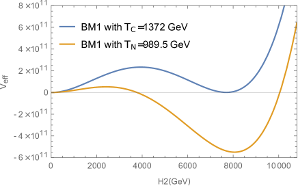
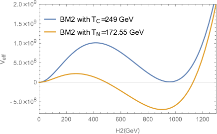
             (a)                                                                     (b)

     

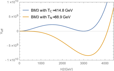
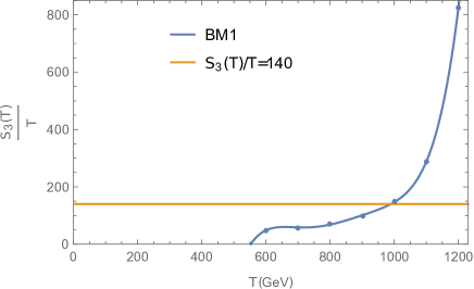
             (c)                                                                     (d)

     

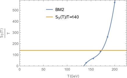
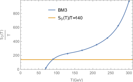
             (e)                                                                     (f)

Figure 5: In (a), (b) and (c) Potential behavior are given for critical temperature and nucleation temperature. In (d), (e) and (f) $S_{3}/T$ changes in terms of temperature are also given for all three benchmarks.

$\#$	$M_{V}(GeV)$	$M_{\psi}(GeV)$	$g_{v}$	$g_{s}$	$M_{H_{2}}(GeV)$	$\Omega_{{\psi}}h^{2}$	$\sigma_{{\psi}}(cm^{2})$
1	4302	220	0.53	0.038	447.9	$1.19\times 10^{-1}$	$3.4\times 10^{-49}$
2	1662	1531	2	2.6	123.5	$1.18\times 10^{-1}$	$7.56\times 10^{-47}$
3	1375	54.89	0.43	0.024	115.4	$1.10\times 10^{-1}$	$2.95\times 10^{-50}$
$\#$	$T_{C}(GeV)$	$T_{N}(GeV)$	$\alpha$	$\beta/H_{\ast}$	$(\Omega_{GW}h^{2})_{max}$
1	1372	989.5	0.047	581.26	$3.13\times 10^{-14}$	—–	—–
2	249	172.55	0.043	1141.97	$1.13\times 10^{-14}$	—–	—–
3	414.8	88.9	4.18	381.52	$3.22\times 10^{-9}$	—–	—–

Table 2: Three benchmark points with DM and phase transition parameters.

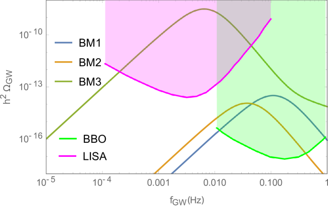
Figure 6: GW spectrum for benchmark points of the table 2.

4 Scenario B

4.1 DM phenomenology

4.1.1 Relic density

In this scenario, $M_{V}<2M_{\psi}$ and both $V_{\mu}$ and $\psi$ fields are considered as DM. The evolution of the number density of DM particles with time are governed by the Boltzmann equation. The coupled Boltzmann equations for fermion ${\psi}$ and vector DM are given by:

$$\frac{dn_{V}}{dt}+3Hn_{V}=-\sum_{j}\langle\sigma_{VV\rightarrow jj}\upsilon\rangle(n_{V}^{2}-n_{V,eq}^{2})-\langle\sigma_{VV\rightarrow{\psi}{\psi}}\upsilon\rangle(n_{V}^{2}-n_{V,eq}^{2}\frac{n_{\psi}^{2}}{n_{{\psi},eq}^{2}}),$$ (4.1)

$$\frac{dn_{\psi}}{dt}+3Hn_{\psi}=-\sum_{j}\langle\sigma_{{\psi}{\psi}\rightarrow jj}\upsilon\rangle(n_{\psi}^{2}-n_{{\psi},eq}^{2})-\langle\sigma_{{\psi}{\psi}\rightarrow VV}\upsilon\rangle(n_{\psi}^{2}-n_{{\psi},eq}^{2}\frac{n_{V}^{2}}{n_{V,eq}^{2}}),$$ (4.2)

where $j$ runs over SM massive particles, $H_{1}$ and $H_{2}$. In $\langle\sigma_{ab\rightarrow cd}\upsilon\rangle$ all annihilations are taken into account except $\langle\sigma_{{\psi}V\rightarrow{\psi}V}\upsilon\rangle$ which does not affect the number density. The relevant Feynman diagrams for DM production are shown in the Figure 7. By choosing $x=M/T$ and $Y=n/s$, , where $T$ and $s$ are the photon temperature and the entropy density respectively, one can rewrite the Boltzmann equations in terms of $Y=n/s$:

$$\frac{dY_{V}}{dx}=-\sqrt{\frac{45}{\pi}}M_{pl}g_{*}^{1/2}\frac{M}{x^{2}}[\sum_{j}\langle\sigma_{VV\rightarrow jj}\upsilon\rangle(Y_{V}^{2}-Y_{V,eq}^{2})+\langle\sigma_{VV\rightarrow{\psi}{\psi}}\upsilon\rangle(Y_{V}^{2}-Y_{V,eq}^{2}\frac{Y_{\psi}^{2}}{Y_{{\psi},eq}^{2}})],$$ (4.3)

$$\frac{dY_{\psi}}{dx}=-\sqrt{\frac{45}{\pi}}M_{pl}g_{*}^{1/2}\frac{M}{x^{2}}[\sum_{j}\langle\sigma_{{\psi}{\psi}\rightarrow jj}\upsilon\rangle(Y_{\psi}^{2}-Y_{{\psi},eq}^{2})+\langle\sigma_{{\psi}{\psi}\rightarrow VV}\upsilon\rangle(Y_{\psi}^{2}-Y_{{\psi},eq}^{2}\frac{Y_{V}^{2}}{Y_{V,eq}^{2}})],$$ (4.4)

where $g_{*}^{1/2}$ is the degrees of freedom parameter and $M_{pl}$ is the Planck mass. It is clear from the above equations that there are new terms in Boltzmann equations which describe the conversion of two DM particles into each other. Because these two cross sections are also described by the same matrix element, we expect $\langle\sigma_{VV\rightarrow{\psi}{\psi}}\upsilon\rangle$ and $\langle\sigma_{{\psi}{\psi}\rightarrow VV}\upsilon\rangle$ are not independent and their relation is:

$$Y_{V,eq}^{2}\langle\sigma_{VV\rightarrow{\psi}{\psi}}\upsilon\rangle=Y_{{\psi},eq}^{2}\langle\sigma_{{\psi}{\psi}\rightarrow VV}\upsilon\rangle.$$ (4.5)

The interactions between the two DM components take place by exchanging two scalar mass eigenstates $H_{1}$ and $H_{2}$ where the coupling of $V$ to $H_{1}$ is suppressed by $\sin\alpha$. For this reason, it usually is the $H_{2}$ -mediated diagram that gives the dominant contribution. We also know that the conversion of the heavier particle into the lighter one is relevant. The relic density for any DM candidate associated with the $Y$ at the present temperature is given by the following relation:

$$\Omega_{{\psi},V}h^{2}=2.755\times 10^{8}\frac{M_{{\psi},V}}{GeV}Y_{{\psi},V}(T_{0})$$ (4.6)

where $h$ is the Hubble expansion rate at present times in units of $100(km/s)/Mpc$. We use the micrOMEGAs package[99] to numerically solve coupled Boltzmann differential equations. According to the data by Planck collaboration[96], the DM constraint in this model reads

$$\Omega_{DM}h^{2}=\Omega_{V}h^{2}+\Omega_{{\psi}}h^{2}=0.120\pm 0.001.$$ (4.7)

We also define the fraction of the DM density of each component by,

$$\xi_{V}=\frac{\Omega_{V}}{\Omega_{DM}},~{}~{}~{}~{}~{}\xi_{\psi}=\frac{\Omega_{{\psi}}}{\Omega_{DM}},~{}~{}~{}\xi_{V}+\xi_{\psi}=1.$$ (4.8)

In Figure 8, the parameter space consistent with DM relic density is obtained. As can be seen, there is an agreement with the relic density observed for $800<M_{V}<5000$ GeV, $500<M_{\psi}<4700$ GeV and $1<g_{v}<6$. On the other hand, according to 2.19 and that the allowed points in figure 8 are above the $M_{V}$=$M_{\psi}$ line, $M_{\psi}$ should be smaller than $M_{V}$, therefore we expect that the dominate DM component is fermionic($V_{\mu}$ includes approximately 1.5% of Relic Density’s share).

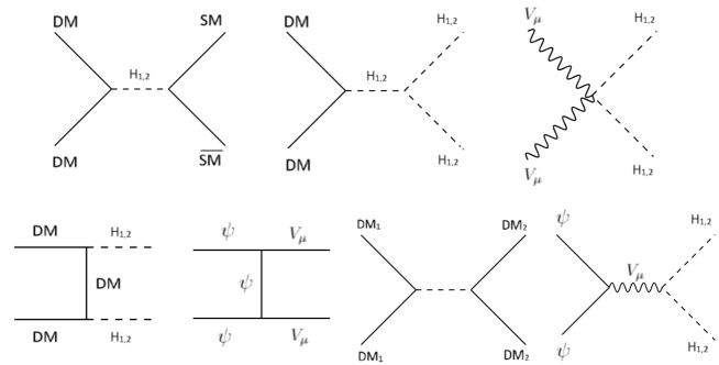
Figure 7: The relevant Feynman diagrams for DM relic density production cross section.

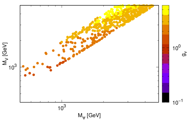
Figure 8: The allowed range of parameter space consistent with DM relic density.

4.1.2 Direct detection

We investigate constraints on parameters space of the model which are imposed by searching for scattering of DM-nuclei. The spin-independent direct detection(DD) cross sections of $V$ and ${\psi}$ are determined by $H_{1}$ and $H_{2}$ exchanged diagrams[69, 30]:

$$\sigma_{DM-N}^{V}=\frac{4\lambda_{SH}^{2}M_{V}^{2}M_{N}^{2}\mu_{VN}^{2}(M_{H1}^{2}-M_{H2}^{2})^{2}}{\pi M_{H1}^{8}M_{H2}^{4}}f_{N}^{2},$$ (4.9)

$$\sigma_{DM-N}^{\psi}=\xi_{\psi}\frac{g_{s}^{3}\nu_{1}}{\pi M_{\psi}(1+(\nu_{1}g_{s}/M_{\psi})^{2})}\mu_{\psi}^{2}(\frac{1}{M_{H1}^{2}}-\frac{1}{M_{H2}^{2}})^{2}f_{N}^{2},$$ (4.10)

where

$$\mu_{VN}=M_{N}M_{V}/(M_{N}+M_{V}),~{}~{}~{}~{}~{}\mu_{\psi}=M_{N}M_{\psi}/(M_{N}+M_{\psi}).$$ (4.11)

$M_{N}$ is the nucleon mass and $f_{N}\simeq 0.3$ parametrizes the Higgs-nucleon coupling.

Various DD experiments have placed constraints on DM-Nucleon spin independent cross section, such as LUX[118], PandaX-II[119], XENON1T[120],LZ[121] and XENONnT[97]. Of course, these experiments are gradually approaching what is called the neutrino floor[122], which is a the irreducible background coming from scattering of SM neutrinos on nucleons. We use the XENONnT[97] experiment results to constrain the parameter space of our model. In this experiment there is a minimum upper limit on the spin-independent WIMP-nucleon cross section of $2.58\times 10^{-47}$ $cm^{2}$ for a WIMP mass of $28$ GeV . In order to study the effect of the direct detection experiment on the model, we use rescaled DM-Nucleon cross section $\xi_{V}\sigma_{V}$ and $\xi_{\psi}\sigma_{\psi}$.

In Figure 9, rescaled DM-Nucleon cross sections($\xi_{V}\sigma_{V}$ and $\xi_{\psi}\sigma_{\psi}$) are depicted for the parameters that are in agreement with the relic density. What is clear from the Figure, there are some points between the XENONnT direct detection bound and the neutrino floor which can be probed in the future direct detection experiments.

     

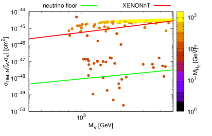
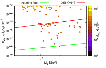
             (a)                                                                     (b)

Figure 9: The allowed range of parameter space consistent with DM relic density and DD. In (a) $\xi_{V}\sigma_{V}$ VS $M_{V}$ and in (b) $\xi_{\psi}\sigma_{\psi}$ VS $M_{\psi}$ has shown.

4.1.3 Invisible Higgs decay

In this scenario, according to figure 9, because there is no point where $M_{\psi,V,H_{2}}<M_{H1}/2$, it is not necessary to check the invisible Higgs decay.

4.2 Electroweak phase transition and gravitational waves

To investigate the phase transition and the resulting GWs, we follow the procedure of Section 3.2. We select three benchmark points as shown in Table 3. The benchmarks 1 and 2 are consistent with direct detection constraint while the benchmark 3 is placed under the neutrino floor. Figure 10 shows the changes of potential and $S_{3}/T$ in terms of temperature. The GW spectrum for these benchmark points is depicted in figure 11. The GW spectrum for these benchmark falls within the observational window of BBO. For the benchmark 3 which is below the neutrino floor limit, future gravitational wave detectors can be a special way to discover and investigate it.

$\#$	$M_{V}(GeV)$	$M_{\psi}(GeV)$	$g_{v}$	$g_{s}$	$M_{H_{2}}(GeV)$
1	1136	1021	1.69	2.15	126.3
2	2207	2045	2.3	3.01	126.2
3	2097	1941	2.26	2.96	124.7
$\#$	$\Omega_{V}h^{2}$	$\Omega_{{\psi}}h^{2}$	$\Omega_{DM}h^{2}$	$\xi_{V}\sigma_{V}(cm^{2})$	$\xi_{{\psi}}\sigma_{{\psi}}(cm^{2})$
1	$1.7\times 10^{-3}$	$1.11\times 10^{-1}$	$1.13\times 10^{-1}$	$1.43\times 10^{-48}$	$7.62\times 10^{-47}$
2	$1.9\times 10^{-3}$	$1.19\times 10^{-1}$	$1.21\times 10^{-1}$	$1.14\times 10^{-48}$	$6.15\times 10^{-47}$
3	$1.83\times 10^{-3}$	$1.14\times 10^{-1}$	$1.16\times 10^{-1}$	$2.3\times 10^{-50}$	$1.23\times 10^{-48}$
$\#$	$T_{C}(GeV)$	$T_{N}(GeV)$	$\alpha$	$\beta/H_{\ast}$	$(\Omega_{GW}h^{2})_{max}$
1	179	137.15	0.02	1352.63	$5.09\times 10^{-16}$
2	470	254.4	0.03	645.6	$5.06\times 10^{-15}$
3	404	252.85	0.01	2850.45	$1.66\times 10^{-17}$

Table 3: Three benchmark points with DM and phase transition parameters.

     

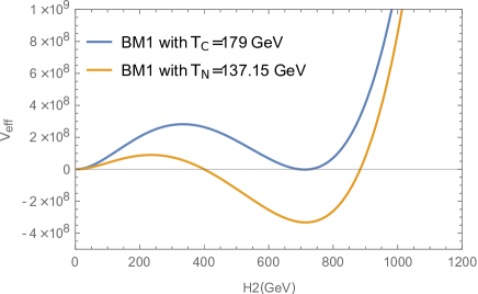
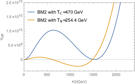
             (a)                                                                     (b)

     

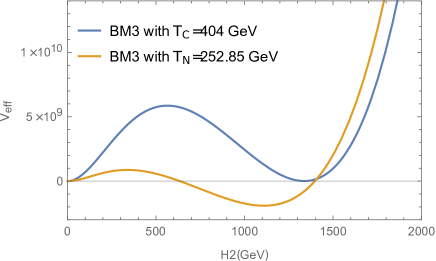
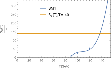
             (c)                                                                     (d)

     

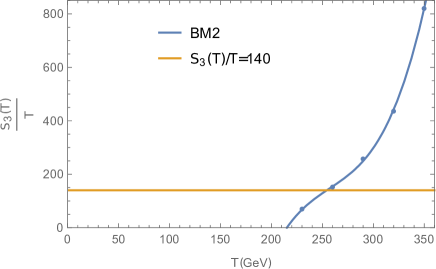
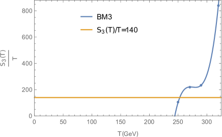
             (e)                                                                     (f)

Figure 10: In (a), (b) and (c) Potential behavior are given for critical temperature and nucleation temperature. In (d), (e) and (f) $S_{3}/T$ changes in terms of temperature are also given for all three benchmarks.

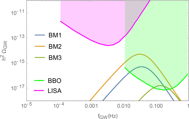
Figure 11: GW spectrum for benchmark points of the table 3.

5 Conclusion

We have considered an extension of the SM with the new $U(1)$ symmetry in the dark part. According to the new particle mass in the model, we considered two different scenarios. The model consists three new fields: a fermion, a complex scalar, and a vector field. In scenario A, only fermionic particle is considered as DM. In scenario B, both vector and fermionic particles are considered as DM. The model has classical scale symmetry and electroweak symmetry breaking occurs through Gildener-Weinberg mechanism and gives a natural solution to the hierarchy problem. Numerical solution of the Boltzmann equations for both scenarios was conducted to determine a parameter space region which is compatible with Planck and XENONnT data and collider constraints (Invisible Higgs decay in scenario A), a three-dimensional parameter space acquisition was completed.

We focused our attention on the phase transition dynamics after presenting the model and exploring DM phenomenology. The full finite-temperature effective potential of the model at one loop level has been obtained to investigate the nature and strength of the electroweak phase transition, with the aim of exploring its nature and strength. A first-order electroweak phase transition can exist when there is a barrier between the broken and symmetric phase. it was demonstrated that the finite-temperature effects induce such an barrier and thereby give rise to a phase transition which can generate GWs.

After studying the phase transition, we investigated the resulting GWs. The parameters required to investigate GWs can all be calculated from our presented model and are a function of the independent parameters of the model. We have demonstrated that the model can survive DM relic density, direct detection and collider constraints, while also producing GWs during the first order electroweak phase transition. We also showed that GWs can be a special probe for the benchmarks that are placed under the neutrino floor(benchmark 3 in both scenarios). These waves can be placed within the observation window of LISA and BBO, which is hoped to be a path to new physics.

References

- [1] G. Bertone and D. Hooper, History of dark matter, Rev. Mod. Phys. 90 (2018) 045002 [1605.04909].
- [2] J. L. Feng, The WIMP Paradigm: Theme and Variations, in Les Houches summer school on Dark Matter, 12, 2022, 2212.02479, DOI.
- [3] K. M. Zurek, Multi-Component Dark Matter, Phys. Rev. D 79 (2009) 115002 [0811.4429].
- [4] S. Profumo, K. Sigurdson and L. Ubaldi, Can we discover multi-component WIMP dark matter?, JCAP 12 (2009) 016 [0907.4374].
- [5] M. Aoki, M. Duerr, J. Kubo and H. Takano, Multi-Component Dark Matter Systems and Their Observation Prospects, Phys. Rev. D 86 (2012) 076015 [1207.3318].
- [6] A. Biswas, D. Majumdar, A. Sil and P. Bhattacharjee, Two Component Dark Matter : A Possible Explanation of 130 GeV Ray Line from the Galactic Centre, JCAP 12 (2013) 049 [1301.3668].
- [7] P.-H. Gu, Multi-component dark matter with magnetic moments for Fermi-LAT gamma-ray line, Phys. Dark Univ. 2 (2013) 35 [1301.4368].
- [8] M. Aoki, J. Kubo and H. Takano, Two-loop radiative seesaw mechanism with multicomponent dark matter explaining the possible excess in the Higgs boson decay and at the Fermi LAT, Phys. Rev. D 87 (2013) 116001 [1302.3936].
- [9] Y. Kajiyama, H. Okada and T. Toma, Multicomponent dark matter particles in a two-loop neutrino model, Phys. Rev. D 88 (2013) 015029 [1303.7356].
- [10] L. Bian, R. Ding and B. Zhu, Two Component Higgs-Portal Dark Matter, Phys. Lett. B 728 (2014) 105 [1308.3851].
- [11] S. Bhattacharya, A. Drozd, B. Grzadkowski and J. Wudka, Two-Component Dark Matter, JHEP 10 (2013) 158 [1309.2986].
- [12] C.-Q. Geng, D. Huang and L.-H. Tsai, Imprint of multicomponent dark matter on AMS-02, Phys. Rev. D 89 (2014) 055021 [1312.0366].
- [13] S. Esch, M. Klasen and C. E. Yaguna, A minimal model for two-component dark matter, JHEP 09 (2014) 108 [1406.0617].
- [14] K. R. Dienes, J. Kumar, B. Thomas and D. Yaylali, Dark-Matter Decay as a Complementary Probe of Multicomponent Dark Sectors, Phys. Rev. Lett. 114 (2015) 051301 [1406.4868].
- [15] L. Bian, T. Li, J. Shu and X.-C. Wang, Two component dark matter with multi-Higgs portals, JHEP 03 (2015) 126 [1412.5443].
- [16] C.-Q. Geng, D. Huang and C. Lai, Revisiting multicomponent dark matter with new AMS-02 data, Phys. Rev. D 91 (2015) 095006 [1411.4450].
- [17] A. DiFranzo and G. Mohlabeng, Multi-component Dark Matter through a Radiative Higgs Portal, JHEP 01 (2017) 080 [1610.07606].
- [18] M. Aoki and T. Toma, Implications of Two-component Dark Matter Induced by Forbidden Channels and Thermal Freeze-out, JCAP 01 (2017) 042 [1611.06746].
- [19] A. Dutta Banik, M. Pandey, D. Majumdar and A. Biswas, Two component WIMP–FImP dark matter model with singlet fermion, scalar and pseudo scalar, Eur. Phys. J. C 77 (2017) 657 [1612.08621].
- [20] M. Pandey, D. Majumdar and K. P. Modak, Two Component Feebly Interacting Massive Particle (FIMP) Dark Matter, JCAP 06 (2018) 023 [1709.05955].
- [21] D. Borah, A. Dasgupta, U. K. Dey, S. Patra and G. Tomar, Multi-component Fermionic Dark Matter and IceCube PeV scale Neutrinos in Left-Right Model with Gauge Unification, JHEP 09 (2017) 005 [1704.04138].
- [22] J. Herrero-Garcia, A. Scaffidi, M. White and A. G. Williams, On the direct detection of multi-component dark matter: sensitivity studies and parameter estimation, JCAP 11 (2017) 021 [1709.01945].
- [23] A. Ahmed, M. Duch, B. Grzadkowski and M. Iglicki, Multi-Component Dark Matter: the vector and fermion case, Eur. Phys. J. C 78 (2018) 905 [1710.01853].
- [24] S. Peyman Zakeri, S. Mohammad Moosavi Nejad, M. Zakeri and S. Yaser Ayazi, A Minimal Model For Two-Component FIMP Dark Matter: A Basic Search, Chin. Phys. C 42 (2018) 073101 [1801.09115].
- [25] M. Aoki and T. Toma, Boosted Self-interacting Dark Matter in a Multi-component Dark Matter Model, JCAP 10 (2018) 020 [1806.09154].
- [26] S. Chakraborti and P. Poulose, Interplay of Scalar and Fermionic Components in a Multi-component Dark Matter Scenario, Eur. Phys. J. C 79 (2019) 420 [1808.01979].
- [27] N. Bernal, D. Restrepo, C. Yaguna and O. Zapata, Two-component dark matter and a massless neutrino in a new model, Phys. Rev. D 99 (2019) 015038 [1808.03352].
- [28] A. Poulin and S. Godfrey, Multicomponent dark matter from a hidden gauged SU(3), Phys. Rev. D 99 (2019) 076008 [1808.04901].
- [29] J. Herrero-Garcia, A. Scaffidi, M. White and A. G. Williams, On the direct detection of multi-component dark matter: implications of the relic abundance, JCAP 01 (2019) 008 [1809.06881].
- [30] S. Yaser Ayazi and A. Mohamadnejad, Scale-Invariant Two Component Dark Matter, Eur. Phys. J. C 79 (2019) 140 [1808.08706].
- [31] F. Elahi and S. Khatibi, Multi-Component Dark Matter in a Non-Abelian Dark Sector, Phys. Rev. D 100 (2019) 015019 [1902.04384].
- [32] D. Borah, A. Dasgupta and S. K. Kang, Two-component dark matter with cogenesis of the baryon asymmetry of the Universe, Phys. Rev. D 100 (2019) 103502 [1903.10516].
- [33] S. Bhattacharya, P. Ghosh, A. K. Saha and A. Sil, Two component dark matter with inert Higgs doublet: neutrino mass, high scale validity and collider searches, JHEP 03 (2020) 090 [1905.12583].
- [34] A. Biswas, D. Borah and D. Nanda, Type III seesaw for neutrino masses in U(1)B-L model with multi-component dark matter, JHEP 12 (2019) 109 [1908.04308].
- [35] D. Nanda and D. Borah, Connecting Light Dirac Neutrinos to a Multi-component Dark Matter Scenario in Gauged Model, Eur. Phys. J. C 80 (2020) 557 [1911.04703].
- [36] C. E. Yaguna and O. Zapata, Multi-component scalar dark matter from a symmetry: a systematic analysis, JHEP 03 (2020) 109 [1911.05515].
- [37] G. Bélanger, A. Pukhov, C. E. Yaguna and O. Zapata, The Z5 model of two-component dark matter, JHEP 09 (2020) 030 [2006.14922].
- [38] P. Van Dong, C. H. Nam and D. Van Loi, Canonical seesaw implication for two-component dark matter, Phys. Rev. D 103 (2021) 095016 [2007.08957].
- [39] S. Khalil, S. Moretti, D. Rojas-Ciofalo and H. Waltari, Multicomponent dark matter in a simplified E6SSM, Phys. Rev. D 102 (2020) 075039 [2007.10966].
- [40] A. Dutta Banik, R. Roshan and A. Sil, Two component singlet-triplet scalar dark matter and electroweak vacuum stability, Phys. Rev. D 103 (2021) 075001 [2009.01262].
- [41] J. Hernandez-Sanchez, V. Keus, S. Moretti, D. Rojas-Ciofalo and D. Sokolowska, Complementary Probes of Two-component Dark Matter, 2012.11621.
- [42] N. Chakrabarty, R. Roshan and A. Sil, Two-component doublet-triplet scalar dark matter stabilizing the electroweak vacuum, Phys. Rev. D 105 (2022) 115010 [2102.06032].
- [43] C. E. Yaguna and O. Zapata, Two-component scalar dark matter in Z2n scenarios, JHEP 10 (2021) 185 [2106.11889].
- [44] B. Díaz Sáez, P. Escalona, S. Norero and A. R. Zerwekh, Fermion singlet dark matter in a pseudoscalar dark matter portal, JHEP 10 (2021) 233 [2105.04255].
- [45] B. Díaz Sáez, K. Möhling and D. Stöckinger, Two real scalar WIMP model in the assisted freeze-out scenario, JCAP 10 (2021) 027 [2103.17064].
- [46] Y. G. Kim, K. Y. Lee and S.-h. Nam, Phenomenology of a two-component dark matter model, Phys. Lett. B 834 (2022) 137412 [2201.11485].
- [47] S.-Y. Ho, P. Ko and C.-T. Lu, Scalar and fermion two-component SIMP dark matter with an accidental symmetry, JHEP 03 (2022) 005 [2201.06856].
- [48] F. Costa, S. Khan and J. Kim, A two-component dark matter model and its associated gravitational waves, JHEP 06 (2022) 026 [2202.13126].
- [49] S. Bhattacharya, P. Ghosh, J. Lahiri and B. Mukhopadhyaya, Mono-X signal and two component dark matter: new distinction criteria, 2211.10749.
- [50] S. Bhattacharya, P. Ghosh, J. Lahiri and B. Mukhopadhyaya, Distinguishing two dark matter component particles at e+e- colliders, JHEP 12 (2022) 049 [2202.12097].
- [51] S. Bhattacharya, P. Ghosh and N. Sahu, Multipartite Dark Matter with Scalars, Fermions and signatures at LHC, JHEP 02 (2019) 059 [1809.07474].
- [52] S. Bhattacharya, P. Poulose and P. Ghosh, Multipartite Interacting Scalar Dark Matter in the light of updated LUX data, JCAP 04 (2017) 043 [1607.08461].
- [53] K. Kajantie, M. Laine, K. Rummukainen and M. E. Shaposhnikov, Is there a hot electroweak phase transition at ?, Phys. Rev. Lett. 77 (1996) 2887 [hep-ph/9605288].
- [54] Y. Aoki, F. Csikor, Z. Fodor and A. Ukawa, The Endpoint of the first order phase transition of the SU(2) gauge Higgs model on a four-dimensional isotropic lattice, Phys. Rev. D 60 (1999) 013001 [hep-lat/9901021].
- [55] D. J. Weir, Gravitational waves from a first order electroweak phase transition: a brief review, Phil. Trans. Roy. Soc. Lond. A 376 (2018) 20170126 [1705.01783].
- [56] M. Chala, G. Nardini and I. Sobolev, Unified explanation for dark matter and electroweak baryogenesis with direct detection and gravitational wave signatures, Phys. Rev. D 94 (2016) 055006 [1605.08663].
- [57] A. Soni and Y. Zhang, Gravitational Waves From SU(N) Glueball Dark Matter, Phys. Lett. B 771 (2017) 379 [1610.06931].
- [58] R. Flauger and S. Weinberg, Gravitational Waves in Cold Dark Matter, Phys. Rev. D 97 (2018) 123506 [1801.00386].
- [59] I. Baldes, Gravitational waves from the asymmetric-dark-matter generating phase transition, JCAP 05 (2017) 028 [1702.02117].
- [60] W. Chao, H.-K. Guo and J. Shu, Gravitational Wave Signals of Electroweak Phase Transition Triggered by Dark Matter, JCAP 09 (2017) 009 [1702.02698].
- [61] A. Beniwal, M. Lewicki, J. D. Wells, M. White and A. G. Williams, Gravitational wave, collider and dark matter signals from a scalar singlet electroweak baryogenesis, JHEP 08 (2017) 108 [1702.06124].
- [62] F. P. Huang and J.-H. Yu, Exploring inert dark matter blind spots with gravitational wave signatures, Phys. Rev. D 98 (2018) 095022 [1704.04201].
- [63] F. P. Huang and C. S. Li, Probing the baryogenesis and dark matter relaxed in phase transition by gravitational waves and colliders, Phys. Rev. D 96 (2017) 095028 [1709.09691].
- [64] E. Madge and P. Schwaller, Leptophilic dark matter from gauged lepton number: Phenomenology and gravitational wave signatures, JHEP 02 (2019) 048 [1809.09110].
- [65] L. Bian and Y.-L. Tang, Thermally modified sterile neutrino portal dark matter and gravitational waves from phase transition: The Freeze-in case, JHEP 12 (2018) 006 [1810.03172].
- [66] L. Bian and X. Liu, Two-step strongly first-order electroweak phase transition modified FIMP dark matter, gravitational wave signals, and the neutrino mass, Phys. Rev. D 99 (2019) 055003 [1811.03279].
- [67] V. R. Shajiee and A. Tofighi, Electroweak Phase Transition, Gravitational Waves and Dark Matter in Two Scalar Singlet Extension of The Standard Model, Eur. Phys. J. C 79 (2019) 360 [1811.09807].
- [68] K. Kannike and M. Raidal, Phase Transitions and Gravitational Wave Tests of Pseudo-Goldstone Dark Matter in the Softly Broken U(1) Scalar Singlet Model, Phys. Rev. D 99 (2019) 115010 [1901.03333].
- [69] S. Yaser Ayazi and A. Mohamadnejad, Conformal vector dark matter and strongly first-order electroweak phase transition, JHEP 03 (2019) 181 [1901.04168].
- [70] A. Mohamadnejad, Gravitational waves from scale-invariant vector dark matter model: Probing below the neutrino-floor, Eur. Phys. J. C 80 (2020) 197 [1907.08899].
- [71] K. Kannike, K. Loos and M. Raidal, Gravitational wave signals of pseudo-Goldstone dark matter in the complex singlet model, Phys. Rev. D 101 (2020) 035001 [1907.13136].
- [72] A. Paul, B. Banerjee and D. Majumdar, Gravitational wave signatures from an extended inert doublet dark matter model, JCAP 10 (2019) 062 [1908.00829].
- [73] B. Barman, A. Dutta Banik and A. Paul, Singlet-doublet fermionic dark matter and gravitational waves in a two-Higgs-doublet extension of the Standard Model, Phys. Rev. D 101 (2020) 055028 [1912.12899].
- [74] D. Marfatia and P.-Y. Tseng, Gravitational wave signals of dark matter freeze-out, JHEP 02 (2021) 022 [2006.07313].
- [75] T. Alanne, N. Benincasa, M. Heikinheimo, K. Kannike, V. Keus, N. Koivunen et al., Pseudo-Goldstone dark matter: gravitational waves and direct-detection blind spots, JHEP 10 (2020) 080 [2008.09605].
- [76] X.-F. Han, L. Wang and Y. Zhang, Dark matter, electroweak phase transition, and gravitational waves in the type II two-Higgs-doublet model with a singlet scalar field, Phys. Rev. D 103 (2021) 035012 [2010.03730].
- [77] Y. Wang, C. S. Li and F. P. Huang, Complementary probe of dark matter blind spots by lepton colliders and gravitational waves, Phys. Rev. D 104 (2021) 053004 [2012.03920].
- [78] X. Deng, X. Liu, J. Yang, R. Zhou and L. Bian, Heavy dark matter and Gravitational waves, Phys. Rev. D 103 (2021) 055013 [2012.15174].
- [79] W. Chao, X.-F. Li and L. Wang, Filtered pseudo-scalar dark matter and gravitational waves from first order phase transition, JCAP 06 (2021) 038 [2012.15113].
- [80] Z. Zhang, C. Cai, X.-M. Jiang, Y.-L. Tang, Z.-H. Yu and H.-H. Zhang, Phase transition gravitational waves from pseudo-Nambu-Goldstone dark matter and two Higgs doublets, JHEP 05 (2021) 160 [2102.01588].
- [81] J. Liu, X.-P. Wang and K.-P. Xie, Searching for lepton portal dark matter with colliders and gravitational waves, JHEP 06 (2021) 149 [2104.06421].
- [82] K. Hashino, M. Kakizaki, S. Kanemura, P. Ko and T. Matsui, Gravitational waves from first order electroweak phase transition in models with the U(1)X gauge symmetry, JHEP 06 (2018) 088 [1802.02947].
- [83] P. Athron, C. Balázs, A. Fowlie, L. Morris and L. Wu, Cosmological phase transitions: from perturbative particle physics to gravitational waves, 2305.02357.
- [84] V. V. Khoze and D. L. Milne, Gravitational waves and dark matter from classical scale invariance, Phys. Rev. D 107 (2023) 095012 [2212.04784].
- [85] E. Witten, Cosmological Consequences of a Light Higgs Boson, Nucl. Phys. B 177 (1981) 477.
- [86] A. H. Guth and E. J. Weinberg, Cosmological Consequences of a First Order Phase Transition in the SU(5) Grand Unified Model, Phys. Rev. D 23 (1981) 876.
- [87] P. J. Steinhardt, The Weinberg-Salam Model and Early Cosmology, Nucl. Phys. B 179 (1981) 492.
- [88] P. J. Steinhardt, Relativistic Detonation Waves and Bubble Growth in False Vacuum Decay, Phys. Rev. D 25 (1982) 2074.
- [89] E. Witten, Cosmic Separation of Phases, Phys. Rev. D 30 (1984) 272.
- [90] LIGO Scientific, Virgo collaboration, Observation of Gravitational Waves from a Binary Black Hole Merger, Phys. Rev. Lett. 116 (2016) 061102 [1602.03837].
- [91] C. Caprini et al., Detecting gravitational waves from cosmological phase transitions with LISA: an update, JCAP 03 (2020) 024 [1910.13125].
- [92] LISA collaboration, Laser Interferometer Space Antenna, 1702.00786.
- [93] J. Crowder and N. J. Cornish, Beyond LISA: Exploring future gravitational wave missions, Phys. Rev. D 72 (2005) 083005 [gr-qc/0506015].
- [94] M. E. Shaposhnikov, Baryon Asymmetry of the Universe in Standard Electroweak Theory, Nucl. Phys. B 287 (1987) 757.
- [95] S. R. Coleman and E. J. Weinberg, Radiative Corrections as the Origin of Spontaneous Symmetry Breaking, Phys. Rev. D 7 (1973) 1888.
- [96] Planck collaboration, Planck 2018 results. VI. Cosmological parameters, Astron. Astrophys. 641 (2020) A6 [1807.06209].
- [97] XENON collaboration, First Dark Matter Search with Nuclear Recoils from the XENONnT Experiment, 2303.14729.
- [98] E. Gildener and S. Weinberg, Symmetry Breaking and Scalar Bosons, Phys. Rev. D 13 (1976) 3333.
- [99] D. Barducci, G. Belanger, J. Bernon, F. Boudjema, J. Da Silva, S. Kraml et al., Collider limits on new physics within micrOMEGAs4.3, Comput. Phys. Commun. 222 (2018) 327 [1606.03834].
- [100] LHC Higgs Cross Section Working Group collaboration, Handbook of LHC Higgs Cross Sections: 1. Inclusive Observables, 1101.0593.
- [101] A. Denner, S. Heinemeyer, I. Puljak, D. Rebuzzi and M. Spira, Standard Model Higgs-Boson Branching Ratios with Uncertainties, Eur. Phys. J. C 71 (2011) 1753 [1107.5909].
- [102] S. Dittmaier et al., Handbook of LHC Higgs Cross Sections: 2. Differential Distributions, 1201.3084.
- [103] O. Brein, A. Djouadi and R. Harlander, NNLO QCD corrections to the Higgs-strahlung processes at hadron colliders, Phys. Lett. B 579 (2004) 149 [hep-ph/0307206].
- [104] LHC Higgs Cross Section Working Group collaboration, Handbook of LHC Higgs Cross Sections: 3. Higgs Properties, 1307.1347.
- [105] CMS collaboration, Search for invisible decays of the Higgs boson produced via vector boson fusion in proton-proton collisions at s=13 TeV, Phys. Rev. D 105 (2022) 092007 [2201.11585].
- [106] ATLAS collaboration, Search for invisible Higgs-boson decays in events with vector-boson fusion signatures using 139 fb-1 of proton-proton data recorded by the ATLAS experiment, JHEP 08 (2022) 104 [2202.07953].
- [107] L. Dolan and R. Jackiw, Symmetry Behavior at Finite Temperature, Phys. Rev. D 9 (1974) 3320.
- [108] M. E. Carrington, The Effective potential at finite temperature in the Standard Model, Phys. Rev. D 45 (1992) 2933.
- [109] M. E. Shaposhnikov, Possible Appearance of the Baryon Asymmetry of the Universe in an Electroweak Theory, JETP Lett. 44 (1986) 465.
- [110] R. Apreda, M. Maggiore, A. Nicolis and A. Riotto, Gravitational waves from electroweak phase transitions, Nucl. Phys. B 631 (2002) 342 [gr-qc/0107033].
- [111] A. Masoumi, K. D. Olum and J. M. Wachter, Approximating tunneling rates in multi-dimensional field spaces, JCAP 10 (2017) 022 [1702.00356].
- [112] D. Bodeker and G. D. Moore, Can electroweak bubble walls run away?, JCAP 05 (2009) 009 [0903.4099].
- [113] S. J. Huber and T. Konstandin, Gravitational Wave Production by Collisions: More Bubbles, JCAP 09 (2008) 022 [0806.1828].
- [114] M. Hindmarsh, S. J. Huber, K. Rummukainen and D. J. Weir, Numerical simulations of acoustically generated gravitational waves at a first order phase transition, Phys. Rev. D 92 (2015) 123009 [1504.03291].
- [115] C. Caprini, R. Durrer and G. Servant, The stochastic gravitational wave background from turbulence and magnetic fields generated by a first-order phase transition, JCAP 12 (2009) 024 [0909.0622].
- [116] C. Caprini et al., Science with the space-based interferometer eLISA. II: Gravitational waves from cosmological phase transitions, JCAP 04 (2016) 001 [1512.06239].
- [117] M. Kamionkowski, A. Kosowsky and M. S. Turner, Gravitational radiation from first order phase transitions, Phys. Rev. D 49 (1994) 2837 [astro-ph/9310044].
- [118] LUX collaboration, Results from a search for dark matter in the complete LUX exposure, Phys. Rev. Lett. 118 (2017) 021303 [1608.07648].
- [119] PandaX-II collaboration, Dark Matter Results from First 98.7 Days of Data from the PandaX-II Experiment, Phys. Rev. Lett. 117 (2016) 121303 [1607.07400].
- [120] XENON collaboration, Dark Matter Search Results from a One Ton-Year Exposure of XENON1T, Phys. Rev. Lett. 121 (2018) 111302 [1805.12562].
- [121] LZ collaboration, First Dark Matter Search Results from the LUX-ZEPLIN (LZ) Experiment, 2207.03764.
- [122] J. Billard, L. Strigari and E. Figueroa-Feliciano, Implication of neutrino backgrounds on the reach of next generation dark matter direct detection experiments, Phys. Rev. D 89 (2014) 023524 [1307.5458].