A macroscopic quantum three-box paradox: finding consistency with weak macroscopic realism

Abstract

The quantum three-box paradox considers a ball prepared in a superposition of being in one of three Boxes. Bob makes measurements by opening either Box 1 or Box 2. After performing some unitary operations (shuffling), Alice can infer with certainty that the ball was detected by Bob, regardless of which box he opened, if she detects the ball after opening Box 3. The paradox is that the ball would have been found with certainty in either box, if that box had been opened. Resolutions of the paradox include that Bob’s measurement cannot be made non-invasively, or else that realism cannot be assumed at the quantum level. Here, we strengthen the case for the former argument, by constructing macroscopic versions of the paradox. Macroscopic realism implies that the ball is in one of the boxes, prior to Bob or Alice opening any boxes. We demonstrate consistency of the paradox with macroscopic realism, if carefully defined (as weak macroscopic realism, wMR) to apply to the system at the times prior to Alice or Bob opening any Boxes, but after the unitary operations associated with preparation or shuffling. By solving for the dynamics of the unitary operations, and comparing with mixed states, we demonstrate agreement between the predictions of wMR and quantum mechanics: The paradox only manifests if Alice’s shuffling combines both local operations (on Box 3) and nonlocal operations, on the other Boxes. Following previous work, the macroscopic paradox is shown to correspond to a violation of a Leggett-Garg inequality, which implies non-invasive measurability, if wMR holds.

I Introduction

The quantum three-box paradox three-box-paradox concerns results inferred for a system at a time intermediate between two times where the system is in a preselected and postselected state abl . The paradox was introduced by Aharonov and Vaidmann and has attracted much interest kastner ; Maroney ; three-box-revisited ; aharonov-disappearing ; e-george-exp ; e-resch-exp ; e-kol-exp ; kirkpatrick-2007 ; kirkpatrick2003 ; leier-spekkens-prl ; liefer-spekkens ; causal-app ; finkelstein ; lv-reply . The paradox involves a ball prepared in a quantum superposition of being in one of the three boxes. Bob makes a measurement by opening either Box 1 or Box 2, to determine whether or not the ball is in the box he opens. Alice then makes specific transformations on the system, by “shuffling” the ball between the boxes. After these operations, she knows that if she detects the ball in the Box 3, then Bob must have detected the ball in the box he opened. The paradox is that the ball would have been found with certainty in either box, if that box had been opened. The paradox can be considered a quantum game, in which Alice can infer that Bob detected a particle with odds not possible classically three-box-revisited ; Maroney .

The three-box paradox raised questions about what quantum effect is involved, and how to understand the paradox kirkpatrick2003 ; kirkpatrick-2007 ; three-box-revisited ; Maroney ; leier-spekkens-prl ; finkelstein ; liefer-spekkens ; lv-reply . One response is to argue that for a system described as a quantum superposition, it cannot be assumed that the system is in one of those states until measured. Hence, it cannot be assumed that the ball is in one of the boxes, prior to the box being opened, and that this is the origin of the paradox. This approach defies the concept of realism. The argument is not so convincing for a macroscopic version of the paradox, where the states of the system are macroscopically distinct. Macroscopic realism (MR) would posit that the ball must be in one of the boxes, irrespective of Alice or Bob opening a box. On the other hand, it could be argued that decoherence prevents the creation of macroscopic superposition states, so that the paradox could not be realised. This motivates the challenge of a macroscopic version of the three-box paradox. The three-box paradox has been experimentally verified, but at microscopic levels only e-george-exp ; e-kol-exp ; e-resch-exp .

In this paper, we present a mesoscopic three-box paradox corresponding to $N$ quanta (the ball) placed in a superposition of being in one of three modes (boxes). We also present a macroscopic paradox in which the states of the system correspond to macroscopically distinct coherent states of a single-mode field. Since macroscopic quantum superposition states have been created cat-states-super-cond ; collapse-revival-super-circuit-1 , we anticipate these predictions could be tested. This motivates consideration of other approaches to explain the paradox consistently with macroscopic realism.

We show in this paper that the three-box paradox can be explained consistently with macroscopic realism, if the definition of macroscopic realism is carefully refined, as weak macroscopic realism manushan-bell-cat-lg ; ghz-cat ; wigner-friend-macro . Following previous work wigner-friend-macro ; ghz-cat ; manushan-bell-cat-lg , weak macroscopic realism (wMR) posits that the outcome of Bob’s or Alice’s measurement in opening any one of the boxes at the time $t_{i}$ is predetermined: each box is either occupied by the ball or not, and the ball is in one of the boxes. The outcome of Alice or Bob opening box $K$ is represented by a variable $\lambda_{K}$ which takes the value $-1$ or $+1$, if the ball is in the box $K$ or not. Weak macroscopic realism posits specifically that prior to Alice or Bob opening the box $K$, this value is fixed, at the time $t_{i}$ once any preparation and unitary transformations (shuffling) involving the box $K$ is completed. We refer to any such transformations involving Box $K$ as “local” to $K$. The definition of wMR also posits that the ball being in a particular box $K$ at the time $t_{i}$ is not affected by any further measurement or shuffling procedure that might occur solely for the other boxes manushan-bell-cat-lg ; ghz-cat ; wigner-friend-macro . Since the boxes may be spatially separated, we refer to such operations as “nonlocal”.

It is important to note that the definition of wMR is not concerned with microscopic details about the state of the ball. Hence, wMR does not posit that the ’state’ of the ball prior to this measurement needs to be a quantum state. In fact, for macroscopic superposition states, it has been argued previously that if the predetermination given by $\lambda$ is valid, it is not possible to associate the ’state’ of the system given by $\lambda$ with a quantum state manushan-bell-cat-lg ; s-cat .

In this paper, we verify consistency with weak macroscopic realism for the results of the paradox, showing that (in this wMR-model) the paradox arises due to disturbance from Bob’s measurement, but a measurable paradoxical effect occurs in the final joint probabilities, only when Alice’s further unitary transformations involve both the local box $K$ and the other nonlocal boxes. We refer to this as a local-nonlocal operation. This allows us to test the predictions of weak macroscopic realism in a potential experiment. The dynamics of Alice’s transformations are modelled by specific interaction Hamiltonians, and are illustrated by the $Q$ function.

Our results support earlier conclusions which emphasize the role of Bob’s measurement disturbance in explaining the paradox leier-spekkens-prl ; Maroney ; causal-app . Maroney pointed out that the conditions under which the paradox occurs are the same as for the set-up to violate a Leggett-Garg inequality Maroney . Leggett-Garg inequalities are derived from the assumptions of macrorealism legggarg . Macrorealism posits macroscopic realism (MR) (that a system with two or more macroscopically-distinct states available to it must be in one of those states) and also macroscopic noninvasive measurability (NIM)$-$ that it is possible to measure which of two macroscopically-distinct states the system is in, with minimal disturbance to the macroscopic dynamics of the system. Violation of the inequalities can therefore arise from a failure of NIM, and be consistent with MR. By illustrating violation of a new class of Leggett-Garg inequality, Maroney argues that the quantum feature of the paradox is measurement disturbance that cannot be explained classically. In this paper, we show that the negation of macrorealism is possible for the macroscopic and mesoscopic versions of the three-box paradox, along the lines proposed by Maroney, thereby illustrating the quantum nature of the proposed experiments. Similarly, Blasiak and Borsuk identify causal structures for the three-box paradox, showing that a realist viewpoint necessitates measurement disturbance in order to maintain consistency with the assumption of realism causal-app .

Our model extends previous work, since a parameter $\alpha$ or $N$ is introduced, which defines the size of the separation of the states of the system, corresponding to the ball being in the Box or not. The disturbance to the system due to Bob’s measurement can be evaluated, by comparing the states before and after. We find that the $Q$ function for the two states becomes identical, as the system becomes macroscopic ($\alpha\rightarrow\infty$). This supports Leggett and Garg’s macrorealism premise that a noninvasive measurement should exist, for a sufficiently large system. However, when we evaluate the predictions for Alice detecting a Ball in Box 3, we find that the difference between the predictions, depending on whether Bob makes a measurement or not, remains macroscopically measurable, even as $\alpha\rightarrow\infty$. The paradoxical results arise from microscopic differences existing at a prior time, similar to a quantum revival.

These results also support the work of Thenabadu et al manushan-bellcats-noon and Thenabadu and Reid manushan-bell-cat-lg ; manushan-cat-lg , who gave predictions for violations of Leggett-Garg and Bell inequalities involving macroscopically distinct coherent states, $|\alpha\rangle$ and $|-\alpha\rangle$. These authors showed how the violations were consistent with wMR, demonstrating similarly that the Bell-nonlocal effect only occurs when the unitary transformations that determine the measurement settings are carried out at both locations (in a local-nonlocal operation) ghz-cat . Similar results are obtained in delayed-choice-cats ; wigner-friend-macro ; ghz-cat .

The layout of the paper is as follows. In Section II, we summarise the three-box paradox. In Section III, we present a mesoscopic paradox where the three boxes are distinct modes, and the ball corresponds to $N$ quanta. A macroscopic (modified) version of the paradox involving macroscopically distinct coherent states (cat states) is presented in Section V. In Sections IV and V, we give the definition of wMR, and show consistency with wMR for both versions of the paradox. The violation of the Leggett-Garg inequalities is demonstrated for the mesoscopic and macroscopic three-box paradox, in Section VI.

II Three box paradox

We first summarise the states, transformations, measurements involved in the paradox three-box-paradox . The system has three boxes and one ball. The state of the ball being in box $k$ is denoted $|k\rangle$. The system is prepared with the ball in box three i.e. in state $|3\rangle$. A unitary transformation $U_{i}$ transforms the initial system into the superposition state

$$|\psi_{1}\rangle=\frac{1}{\sqrt{3}}(|1\rangle+|2\rangle+|3\rangle)$$ (1)

at time $t_{1}$, so that $U_{i}|3\rangle=|\psi_{1}\rangle$. Using the basis set $\{|1\rangle,$ $|2\rangle$, $|3\rangle$}, we find

$$U_{i} = \frac{1}{\sqrt{6}}\left(\begin{array}[]{ccc}\sqrt{3}&1&\sqrt{2}\\ \sqrt{3}&1&\sqrt{2}\\ 0&2&\sqrt{2}\end{array}\right)$$ (5)

where the basis states $|k\rangle$ correspond to column matrices $(a_{j1})$ with coefficients given as $a_{j1}=\delta_{jk}$. The transformation can be carried out by first applying

$$U_{1i}=\frac{1}{\sqrt{3}}\left(\begin{array}[]{ccc}\sqrt{3}&0&0\\ 0&1&\sqrt{2}\\ 0&\sqrt{2}&1\end{array}\right)$$ (6)

to create the superposition $\sqrt{\frac{2}{3}}|2\rangle+\frac{1}{\sqrt{3}}|3\rangle$, and then applying

$$U_{2i}=\frac{1}{\sqrt{2}}\left(\begin{array}[]{ccc}-1&1&0\\ 1&1&0\\ 0&0&\sqrt{2}\end{array}\right)$$ (7)

to create the superposition $\frac{1}{\sqrt{2}}(|2\rangle+|1\rangle)$ from $|2\rangle$. Hence, $U_{i}=U_{2i}U_{1i}$.

Now, Bob can make a measurement to determine whether the system is in $|1\rangle$ (the ball in box 1), or not. Assuming Bob makes an ideal projective measurement, the state of the system after the measurement according to quantum mechanics is $|1\rangle$ if he detects the ball in box 1. Otherwise, the system is in the superposition state $\frac{1}{\sqrt{2}}(|2\rangle+|3\rangle)$. Alternatively, Bob may make a measurement to determine if the system is in state $|2\rangle$ (the ball is in box 2), or not. Assuming an ideal projective measurement, the state of the system after the measurement according to quantum mechanics is $|2\rangle$ if he detects the ball in box 2. Otherwise, the system is in the superposition state $\frac{1}{\sqrt{2}}(|1\rangle+|3\rangle)$.

After the interactions given by Bob’s measurements, at time $t_{2}$, Alice makes further measurements, to postselect for the state

$$|\psi_{f}\rangle=\frac{1}{\sqrt{3}}(|1\rangle+|2\rangle-|3\rangle)$$ (8)

which is orthogonal to both $\frac{1}{\sqrt{2}}(|2\rangle+|3\rangle)$ and $\frac{1}{\sqrt{2}}(|1\rangle+|3\rangle)$. The measurement is realised as a transformation $U_{f}$, so that $|\psi_{f}\rangle$ maps to $|3\rangle$, at the time $t_{3}$. Alice then performs the postselection by determining whether the ball is in box 3 at the time $t_{3}$. $U_{f}$ has the property that its inverse satisfies

$$U_{f}^{-1}|3\rangle=|\psi_{f}\rangle$$ (9)

To find $U_{f}$, we follow the above procedure and first apply the unitary transformation $U_{1f}$ that transforms $|3\rangle$ into the superposition $\sqrt{\frac{2}{3}}|2\rangle-\frac{1}{\sqrt{3}}|3\rangle$. Then we create superposition $\frac{1}{\sqrt{2}}(|2\rangle+|1\rangle)$ from $|2\rangle$, which defines $U_{2f}=U_{2i}$. We find

$$U_{1f}=\frac{1}{\sqrt{3}}\left(\begin{array}[]{ccc}\sqrt{3}&0&0\\ 0&1&\sqrt{2}\\ 0&\sqrt{2}&-1\end{array}\right)$$ (10)

Hence, $U_{f}^{-1}=U_{2f}U_{1f}$. Hence, the required transformation is $U_{f}=U_{1f}^{-1}U_{2f}^{-1}$ which, noting the transformations are unitary so that $U_{2f}^{-1}=U_{2f}$ and $U_{1f}^{-1}=U_{1f}$, becomes $U_{f}^{-1}|3\rangle=|\psi_{f}\rangle$. Hence, Alice’s transformation is

$$U_{f} = \frac{1}{\sqrt{6}}\left(\begin{array}[]{ccc}-\sqrt{3}&\sqrt{3}&0\\ 1&1&2\\ \sqrt{2}&\sqrt{2}&-\sqrt{2}\end{array}\right)$$ (14)

If after his measurements Bob determines the system to be in $|1\rangle$, then the output after Alice’s transformations is

$$U_{f}|1\rangle = \frac{1}{\sqrt{6}}\left(\begin{array}[]{c}-\sqrt{3}\\ 1\\ \sqrt{2}\end{array}\right)$$ (18)

If Bob measures that the system is not in $|1\rangle$, then the output after Alice’s operations is

$$U_{f}\frac{1}{\sqrt{2}}\left(\begin{array}[]{c}0\\ 1\\ 1\end{array}\right) = \frac{1}{2\sqrt{3}}\left(\begin{array}[]{c}\sqrt{3}\\ 3\\ 0\end{array}\right)$$ (25)

If after his measurements Bob determined the system to be in $|2\rangle$, then the final state is

$$U_{f}|2\rangle = \frac{1}{\sqrt{6}}\left(\begin{array}[]{c}\sqrt{3}\\ 1\\ \sqrt{2}\end{array}\right)$$ (29)

If Bob measures that the system is not in $|2\rangle$, then the final state is

$$U_{f}\frac{1}{\sqrt{2}}\left(\begin{array}[]{c}1\\ 0\\ 1\end{array}\right) = \frac{1}{2\sqrt{3}}\left(\begin{array}[]{c}-\sqrt{3}\\ 3\\ 0\end{array}\right)$$ (36)

We see that if Bob determines that the system is not in state $|1\rangle$ (or $|2\rangle)$, then the probability of Alice determining that the system is in state $|3\rangle$ at time $t_{3}$ is zero. Whenever Alice measures that the ball is in Box 3 (i.e. when she confirms the system at time $t_{3}$ is in the state $|3\rangle$), it is certain that Bob found the ball in the box he measured. This leads to the paradox.

The measured probabilities for the paradox can be summarised. We follow the notation where $I_{k}$ represents the ball is in Box I at time $t_{k}$. The probabilities for detection of a Ball if Bob opens the Box 1 is $P_{B1}(1_{2})=1/3$. Similarly, $P_{B2}(2_{2})=1/3$. From (18), if Bob detects the ball in Box 1, then $P_{B1}(3_{3}|1_{2})=1/3$. If Bob opens Box 1, the joint probabilities are $P_{B1}(1_{2},3_{3})=P_{B1}(3_{3}|1_{2})P_{B1}(1_{2})=1/9$. Also, if Bob opens Box 1, then $P_{B1}(3_{3})=1/9$. Hence, $P_{B1}(1_{2}|3_{3})=1$. Similarly, if Bob opens Box 2, the probability of him detecting the ball given Alice detects a Ball in Box 3 is $P_{B2}(2_{2}|3_{3})=1$. We find

$$P_{B1}(1_{2}|3_{3})=P_{B2}(2_{2}|3_{3})=1$$ (37)

If there is no measurement by Bob, then the final state at time $t_{3}$ after Alice’s operations is

$$U_{f}|\psi_{1}\rangle = \frac{1}{3\sqrt{2}}\left(\begin{array}[]{c}0\\ 4\\ \sqrt{2}\end{array}\right)$$ (41)

The probability of Alice detecting a ball if Bob makes no measurement is $P_{N}(3_{3})=1/9$. We note that

$$P_{N}(3_{3})=P_{B1}(3_{3})=P_{B2}(3_{3})=1/9$$ (42)

Hence, the probability that Alice detects the ball in Box 3 is not changed by Bob making a measurement. Maroney referred to such a measurement as operationally nondisturbing Maroney , since Alice cannot detect Bob’s inteference, if she is restricted to opening Box 3. On the other hand, if Bob makes a measurement, then the final state on average after Alice’s transformations will be the mixture

$$\rho_{mix,m} = \frac{1}{6}U_{f}|1\rangle\langle 1|U_{f}^{\dagger}+\frac{2}{6}U_{f}(\frac{|2\rangle+|3\rangle}{\sqrt{2}})(\frac{\langle 2|+\langle 3|}{\sqrt{2}})U_{f}^{\dagger}$$

$$+\frac{1}{6}U_{f}|2\rangle\langle 2|U_{f}^{\dagger}+\frac{2}{6}U_{f}(\frac{|1\rangle+|3\rangle}{\sqrt{2}})(\frac{\langle 1|+\langle 3|}{\sqrt{2}})U_{f}^{\dagger}$$

The relative probabilities for Alice detecting the Ball in Box 1, 2 or 3 if Bob makes a measurement are $1/3$, $5/9$ and $1/9$, compared to $0,8/9,1/9$ given by (41), if Bob makes no measurement. We see that overall, the probabilities are changed.

III Mesoscopic paradox

A macroscopic version of the paradox can be constructed by considering that the three states $|1\rangle$, $|2\rangle$ and $|3\rangle$ become macroscopically distinct. It is also necessary to identify suitable unitary transformations. Macroscopic and mesoscopic versions can be constructed in a number of ways. In this section, we first consider a mesoscopic example which is a direct mapping of the original three-box paradox, with the generalisation that the “particle” comprises $N$ quanta. In Section V, we consider a macroscopic example involving coherent states of a single-mode field, which allows a greater depth of study of the dynamics associated with the unitary operations.

III.1 Number states

We analyse a proposal that maps directly onto the original paradox described in Section II, where the three boxes correspond to spatially separated modes. We let

$$|1\rangle = |N\rangle_{1}|0\rangle_{2}|0\rangle_{3}$$

$$|2\rangle = |0\rangle_{1}|N\rangle_{2}|0\rangle_{3}$$

$$|3\rangle = |0\rangle_{1}|0\rangle_{2}|N\rangle_{3}$$ (44)

where $|N\rangle$ is a number state. The state $|n\rangle_{i}$ of the $i$th mode is denoted by the subscript $i=1,2,3$. The subscript is omitted where the meaning is clear. The modes are prepared in the superposition state

$$|\psi_{sup}\rangle\equiv|\psi_{1}\rangle=\frac{e^{i\varphi}}{\sqrt{3}}(|3\rangle+e^{i\varphi_{1}}(i|2\rangle-|1\rangle)$$ (45)

where $\varphi$ and $\varphi_{1}$ are phase shifts, and the modes spatially separated. These states are tripartite extensions of NOON states noon-dowling-1 .

The unitary transformations necessary for the three-box paradox are achieved by an interaction $H_{kl}$ that transforms the state $|N\rangle_{k}|0\rangle_{l}$ into the superposition nonlinear-Ham-1 ; josHam-collett-steel-2-1 ; manushan-bellcats-noon ; carr-two-well

$$e^{i\varphi(\theta)}(\cos\theta|N\rangle_{k}|0\rangle_{l}-i\sin\theta|0\rangle_{k}|N\rangle_{l})$$ (46)

and also the state $|0\rangle_{k}|N\rangle_{l}$ into

$$e^{i\varphi^{\prime}(\theta)}(\sin\theta|N\rangle_{k}|0\rangle_{l}+i\cos\theta|0\rangle_{k}|N\rangle_{l})$$ (47)

For $N=1$, this is achieved by beam splitters or polarising beam splitters. For $N\geq 1$, we use the Josephson interaction that couples modes $k$ and $l$, given as

$$H_{kl}=\kappa(\hat{a}_{k}^{\dagger}\hat{a}_{l}+\hat{a}_{k}\hat{a}_{l}^{\dagger})+g\hat{a}_{k}^{\dagger 2}\hat{a}_{k}^{2}+g\hat{a}_{l}^{\dagger 2}\hat{a}_{l}^{2}$$ (48)

so that $U=e^{-iH_{kl}t/\hbar}$. Calculations have shown the result (46) to be realised to an excellent approximation, for $N\lesssim 100$, to the extent that Bell violations are predicted for systems where the spin states $|\uparrow\rangle$ and $|\downarrow\rangle$ become the mesoscopically distinct states $|N\rangle_{k}|0\rangle_{l}$ and $|0\rangle_{k}|N\rangle_{l}$ manushan-bellcats-noon . Here, $\hat{a}_{k}$, $\hat{a}_{l}$ are the boson destruction operators for two field modes $k$ and $l$, and $\kappa$ and $g$ are the interaction constants. The $\theta$ is a function of the interaction time $t$ and can be selected so that $0\leq\theta\leq 2\pi$. We introduce a scaled time $\theta=\omega_{N}t$ where solutions are given in carr-two-well . Here, we determine $\theta$ numerically, by solving for the time $T_{NOON}$ taken for the system to evolve from $|N\rangle_{k}|0\rangle_{l}$ to (46) where $\theta=\pi/4$. The solutions illustrating (46) are shown in Figure 1.

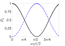
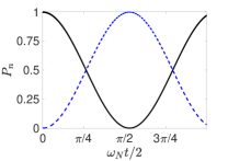
Figure 1: Realisation of a nonlinear beam splitter: Solutions are shown for the Hamiltonian $H_{kl}$ after a time $t$ with initial state $|N\rangle_{k}|0\rangle_{l}$. Top: $N=2$, $\kappa=1$, $g=30$ (left), and $N=5$, $\kappa=20$, $g=333.33$ (right). $P_{N}$ (black solid line) is the probability for all $N$ bosons to be in mode $a_{k}$; $P_{0}$ (blue dashed line) is the probability for all $N$ bosons to be in mode $a_{l}$. The parameters identify regimes optimal, or nearly optimal, for the nonlinear beam splitter interaction, where $P_{N}+P_{0}\sim 1$ and $P_{N}\sim\cos^{2}\omega_{N}t$.

The state $|\psi_{sup}\rangle$ is created from state $|3\rangle$ using the interaction $H_{kl}$ as follows. We define $U_{f}$ so that

$$U_{f}|\psi_{f}\rangle = |3\rangle$$

$$U_{f}^{-1}|3\rangle = |\psi_{f}\rangle$$ (49)

where $|\psi_{f}\rangle$ will be the postselected state. First, we examine how to create the initial superposition state $|\psi_{sup}\rangle$ from $|3\rangle$ i.e. we find $U_{i}$ such that $U_{i}|3\rangle=|\psi_{sup}\rangle$. The state

$$|\psi_{2i}\rangle=e^{i\varphi}(\frac{1}{\sqrt{3}}|3\rangle+i\sqrt{\frac{2}{3}}|2\rangle)$$ (50)

is first created from the initial state $|3\rangle$ by evolving with $H_{32}$ for a suitable time $t_{1i}$, given by $\theta=\omega_{N}t_{1i}=\cos^{-1}(1/\sqrt{3})$ where $3\pi/2<\theta<2\pi$. We find $U_{1i}|3\rangle=e^{-iH_{32}t_{1i}/\hbar}|3\rangle$ where

$$U_{1i}=\frac{1}{\sqrt{3}}\left(\begin{array}[]{ccc}\sqrt{3}&0&0\\ 0&-ie^{i\varphi}&ie^{i\varphi}\sqrt{2}\\ 0&e^{i\varphi}\sqrt{2}&e^{i\varphi}\end{array}\right)$$ (51)

Then the interaction $H_{21}$ for the time $t_{2i}$ given by $\theta=\omega_{N}t_{2}=7\pi/4$ creates $|2\rangle\rightarrow\frac{e^{i\varphi_{1}}}{\sqrt{2}}(|2\rangle+i|1\rangle)$, to give

$$|\psi_{sup}\rangle=\frac{e^{i\varphi}}{\sqrt{3}}(|3\rangle+e^{i\varphi_{1}}(i|2\rangle-|1\rangle)$$ (52)

We find $U_{2i}|\psi_{2i}\rangle=e^{-iH_{21}t_{2i}/\hbar}|\psi_{2i}\rangle$ where

$$U_{2i}=\frac{1}{\sqrt{2}}\left(\begin{array}[]{ccc}-ie^{i\varphi_{1}}&ie^{i\varphi_{1}}&0\\ e^{i\varphi_{1}}&e^{i\varphi_{1}}&0\\ 0&0&\sqrt{2}\end{array}\right)$$ (53)

We find

$$U_{i} = U_{2i}U_{1i}$$ (57)

$$= \frac{1}{\sqrt{6}}\left(\begin{array}[]{ccc}-i\sqrt{3}e^{i\varphi_{1}}&e^{i\varphi_{1}}e^{i\varphi}&i\sqrt{2}e^{i\varphi_{1}}e^{i\varphi}\\ e^{i\varphi_{1}}\sqrt{3}&-ie^{i\varphi_{1}}e^{i\varphi}&ie^{i\varphi_{1}}\sqrt{2}e^{i\varphi}\\ 0&2e^{i\varphi}&\sqrt{2}e^{i\varphi}\end{array}\right)$$

Hence

$$U_{i}^{\dagger}=\frac{1}{\sqrt{6}}\left(\begin{array}[]{ccc}i\sqrt{3}e^{-i\varphi_{1}}&e^{-i\varphi_{1}}\sqrt{3}&0\\ e^{-i\varphi_{1}}e^{-i\varphi}&ie^{-i\varphi}e^{-i\varphi_{1}}&2e^{-i\varphi}\\ -\sqrt{2}e^{-i\varphi_{1}}e^{-i\varphi}&-i\sqrt{2}e^{-i\varphi_{1}}e^{-i\varphi}&\sqrt{2}e^{-i\varphi}\end{array}\right)$$ (58)

The dynamics arising from the Hamiltonians $H_{32}$ and $H_{21}$ for actual values of $g$ and $\kappa$ does not in general constrain the system to the states $|1\rangle$, $|2\rangle$ or $|3\rangle.$ Full solutions are depicted in Figure 2. For the parameters given, the probability that the system is found in a state different to $|1\rangle$, $|2\rangle$ or $|3\rangle$ is however negligible.

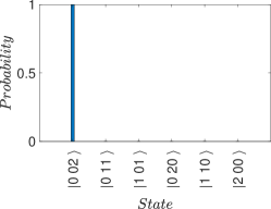
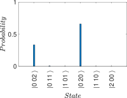
Figure 2: Creation of the superposition $|\psi_{sup}\rangle$ from $|3\rangle$, for $N=2$. The values of $\kappa$ and $g$ are chosen as in Figure 1. Each sequence shows the initial state $|3\rangle$ (far left), the intermediate state $U_{1i}|3\rangle$ (centre), and the final state $U_{2i}U_{1i}|3\rangle$ (far right), where $U_{1i}=e^{-iH_{32}t_{1i}/\hbar}$ and $U_{2i}=e^{-iH_{21}t_{2i}/\hbar}$ for suitable choices of times $t_{1i}$ and $t_{2i}$. Depicted is the probability the system is in state $|k,l,m\rangle\equiv|k\rangle_{1}|l\rangle_{2}|m\rangle_{3}$ at the given time in the sequence. The probability that the system is in a state different to $|1\rangle$, $|2\rangle$ or $|3\rangle$ is less than $3\times 10^{-3}$.

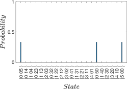
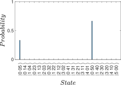
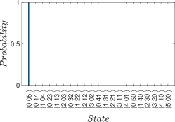
Figure 3: Creation of the superposition $|3\rangle$ from the postselected state $|\psi_{f}\rangle$ using the operations $U_{f}$, for $N=5$. The values of $\kappa$ and $g$ are chosen as in Figure 1. Each sequence shows the initial state $|\psi_{f}\rangle$ (far left), the intermediate state $U_{2f}^{-1}|\psi_{f}\rangle$ (centre), and the final state $U_{1f}^{-1}U_{2f}^{-1}|\psi_{f}\rangle$ (far right), where $U_{1f}\equiv U_{32}$ and $U_{2f}\equiv U_{21}$ as defined in the text. Depicted is the probability the system is in state $|k,l,m\rangle\equiv|k\rangle_{1}|l\rangle_{2}|m\rangle_{3}$ at the given time in the sequence. The probability that the system is in a state different to $|1\rangle$, $|2\rangle$ or $|3\rangle$ is less than $6\times 10^{-3}$.

Now reversing, we see that the postselected state

$$|\psi_{f}\rangle=\frac{e^{i\varphi}}{\sqrt{3}}(-|3\rangle+e^{i\varphi_{1}}(i|2\rangle-|1\rangle))$$ (59)

can be created from $|3\rangle$ using $U_{f}^{-1}$, by applying $H_{32}$ with $\theta=\omega_{N}t$, so that $\cos\theta=-\frac{1}{\sqrt{3}}$, $\sin\theta=-\sqrt{2/3}$, followed by $H_{21}$. We start with $|3\rangle$ and act with $U_{1f}=U_{32}=e^{-iH_{32}t/\hbar}$, for $t=\theta/\omega_{N}$, so that where

$$U_{1f}=\frac{1}{\sqrt{3}}\left(\begin{array}[]{ccc}\sqrt{3}&0&0\\ 0&-ie^{i\varphi}&ie^{i\varphi}\sqrt{2}\\ 0&-e^{i\varphi}\sqrt{2}&-e^{i\varphi}\end{array}\right)$$ (60)

Here,

$$U_{1f}^{\dagger}=\frac{1}{\sqrt{3}}\left(\begin{array}[]{ccc}\sqrt{3}&0&0\\ 0&ie^{-i\varphi}&-e^{-i\varphi}\sqrt{2}\\ 0&-ie^{-i\varphi}\sqrt{2}&-e^{-i\varphi}\end{array}\right)$$

This creates state $|\psi_{1f}\rangle=\frac{e^{i\varphi}}{\sqrt{3}}(-|3\rangle+i\sqrt{2}|2\rangle)$. Then we act on $|\psi_{1f}\rangle$ with $U_{2f}=U_{21}=e^{-iH_{21}t/\hbar}$ for $t$ such that $t=7\pi/4\omega_{N}$ so that $U_{2f}=U_{2i}$. We see that

$$U_{f}^{-1} = U_{2f}U_{1f}$$ (64)

$$= \frac{1}{\sqrt{6}}\left(\begin{array}[]{ccc}-i\sqrt{3}e^{i\varphi_{1}}&e^{i\varphi_{1}}e^{i\varphi}&-e^{i\varphi_{1}}e^{i\varphi}\sqrt{2}\\ \sqrt{3}e^{i\varphi_{1}}&-ie^{i\varphi_{1}}e^{i\varphi}&ie^{i\varphi}e^{i\varphi_{1}}\sqrt{2}\\ 0&-2e^{i\varphi}&-\sqrt{2}e^{i\varphi}\end{array}\right)$$

This gives state $|\psi_{f}\rangle$. Hence, $U_{f}^{-1}|3\rangle=|\psi_{f}\rangle$ where $U_{f}^{-1}=U_{2f}U_{1f}$. Hence, $U_{f}=U_{1f}^{\dagger}U_{2f}^{\dagger}$. Hence, Alice’s measurements are $U_{2f}^{-1}$ followed by $U_{1f}^{-1}$. This gives $U_{f}|\psi_{f}\rangle=|3\rangle$. We find

$$U_{f} = \frac{1}{\sqrt{6}}\left(\begin{array}[]{ccc}i\sqrt{3}e^{-i\varphi_{1}}&\sqrt{3}e^{-i\varphi_{1}}&0\\ e^{-i\varphi_{1}}e^{-i\varphi}&ie^{-i\varphi_{1}}e^{-i\varphi}&-2e^{-i\varphi}\\ -e^{-i\varphi_{1}}e^{-i\varphi}\sqrt{2}&-ie^{-i\varphi}e^{-i\varphi_{1}}\sqrt{2}&-\sqrt{2}e^{-i\varphi}\end{array}\right)$$ (69)

Full solutions are depicted in Figure 3.

The paradox follows as for the original paradox. Bob determines whether the system is in state $|1\rangle$ or not. Alternatively, he determines whether the system is in state $|2\rangle$, or not. If after Bob’s measurements the system is in state $|1\rangle$, then after Alice’s measurements the system is in

$$U_{f}|1\rangle=\frac{e^{-i\varphi_{1}}}{\sqrt{6}}\left(\begin{array}[]{c}i\sqrt{3}\\ e^{-i\varphi}\\ -e^{-i\varphi}\sqrt{2}\end{array}\right)$$ (71)

The solutions in Figure 4 for the optimal choice of $\kappa$ and $g$ give agreement for $N=2$. Similarly, if Bob determines that the system is in state $|2\rangle$, then after Alice’s measurements the system is in

$$U_{f}|2\rangle=\frac{e^{-i\varphi_{1}}}{\sqrt{6}}\left(\begin{array}[]{c}\sqrt{3}\\ ie^{-i\varphi}\\ -ie^{-i\varphi}\sqrt{2}\end{array}\right)$$ (72)

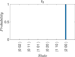
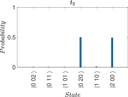
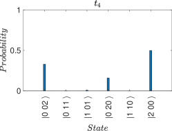
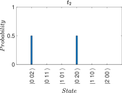
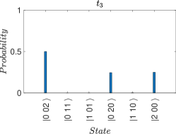
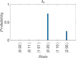
Figure 4: The dynamics corresponding to Alice’s transformations $U_{f}$ if (top row): Bob detects $N$ photons in Box 1 at time $t_{2}$ (top row); or (lower row), if Bob detects the photons are not in Box 1 at time $t_{2}$. The histograms give the probabilities for detecting $N$ photons in Box $k$. Depicted is the probability the system is in state $|k,l,m\rangle\equiv|k\rangle_{1}|l\rangle_{2}|m\rangle_{3}$ at the given time in the sequence. Here, we show the initial state after Bob’s measurement, at time $t_{2}$ (far left), the state generated at time $t_{3}$ after Alice’s transformation $U_{2f}^{-1}$ (centre), and the state generated at time $t_{4}$ after Alice’s further transformation $U_{1f}^{-1}$ (far right). The final state after Alice’s total transformation $U_{f}$ is (71) to an excellent approximation. The probability that the system is in any other state apart from $|00N\rangle$, $|0N0\rangle$ or $|N00\rangle$ is less than $8\times 10^{-3}$. The solutions are for $N=2$. .

If Bob determines the system is not in $|1\rangle$, then at time $t_{2}$ the system is in $(|3\rangle+e^{i\varphi_{1}}i|2\rangle)/\sqrt{2}$. The final state after Alice’s transformations is

$$U_{f}\frac{1}{\sqrt{2}}\left(\begin{array}[]{c}0\\ ie^{i\varphi_{1}}\\ 1\end{array}\right) = \frac{1}{2\sqrt{3}}\left(\begin{array}[]{c}\sqrt{3}\\ -3e^{-i\varphi}\\ 0\end{array}\right)$$ (79)

This is depicted in Figure 4. If Bob determines the system is not in $|2\rangle$, then at time $t_{2}$ the system is in $(|3\rangle-e^{i\varphi_{1}}|1\rangle)/\sqrt{2}$. The final state after Alice’s transformations is

$$U_{f}\frac{1}{\sqrt{2}}\left(\begin{array}[]{c}-e^{i\varphi_{1}}\\ 0\\ 1\end{array}\right) = \frac{1}{2\sqrt{3}}\left(\begin{array}[]{c}-i\sqrt{3}\\ -3e^{-i\varphi}\\ 0\end{array}\right)$$ (86)

The paradox occurs because Alice finds that there is zero probability of finding the system in the state $|3\rangle$ in both cases.

The calculations for the marginal and joint probabilities follows along the same lines as in Section II for the original paradox. We note that if there is no measurement by Bob, then the final state at time $t_{3}$ is

$$U_{f}|\psi_{sup}\rangle = \frac{1}{3\sqrt{2}}\left(\begin{array}[]{c}0\\ -4\\ \sqrt{2}\end{array}\right)$$ (90)

This implies $P_{N}(3_{3})=1/9$. As for the original paradox, this agrees with the value of $P_{B1}(3^{3})=1/9$, calculated from the above results, where Bob opens Box 1. Similarly, $P_{B2}(3^{3})=1/9$. Hence,

$$P_{B1}(1_{2}|3_{3})=1,P_{B2}(2_{2}|3_{3})=1$$

If Bob makes a measurement, the system reduces to the mixture corresponding to the outcomes obtained by Bob. Overall, if he opens Box 1, the state is

$$\rho_{mix,1}(t_{3}) = \frac{1}{3}U_{f}|1\rangle\langle 1|U_{f}^{\dagger}$$

$$+\frac{1}{3}U_{f}(|3\rangle+e^{i\varphi_{1}}i|2\rangle)(\langle 3|-ie^{-i\varphi_{1}}\langle 2|)U_{f}^{\dagger}$$

Similarly, if he opens Box 2, the state is

$$\rho_{mix,2}(t_{3}) = \frac{1}{3}U_{f}|2\rangle\langle 2|U_{f}^{\dagger}$$

$$+\frac{1}{3}U_{f}(|3\rangle-e^{i\varphi_{1}}|2\rangle)(\langle 3|-e^{i\varphi_{1}}\langle 2|)U_{f}^{\dagger}$$

We emphasize that the solution (46) for the evolution given by $H$ is approximate. Actual solutions are given in the figures, and are sufficient to confirm the three-box paradox for moderate $N$, illustrated by $N=2$ and $N=5$.

IV Consistency with weak macroscopic realism: three mode example

By definition, macroscopic realism posits that the system described by the macroscopic superposition states $|\psi_{k}\rangle$ at time $t_{k}$ can be described by a set of values $\lambda_{i}^{(k)}$ which determines the outcome of $\hat{n}_{i}$ for each mode manushan-bell-cat-lg . The variable $\lambda_{i}^{(k)}$ assumes the values $+1$ or $-1$: $1$ indicates the outcome to be $N$; $-1$ indicates the outcome to be $0$.

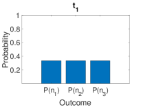
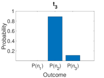
Figure 5: Measurable macroscopic differences occur for the probabilities of outcomes at time $t_{3}$, depending on whether Bob makes a measurement or not, but the differences emerge only after the dynamics of Alice’s operations (shuffling). This gives consistency with weak macroscopic realism. Plotted are the probabilities $P(n_{k})$ of obtaining $N$ on measuring $\hat{n}$ of mode $k$ at the time $t$. The top sequence shows the sequence of probabilities if Bob makes no measurement. The lower sequence shows the probabilities if Bob makes a measurement between times $t_{1}$ and $t_{2}$. The far right plots show the probabilities at time $t_{3}$, after Alice’s operation $U_{f}$, which takes place between times $t_{2}$ and $t_{3}$.

If it is assumed that macroscopic realism holds, then how does the three-box paradox occur? We solve for the dynamics as Bob and Alice make their measurements, which includes the unitary transformations $U$. At the times $t_{1}$, $t_{2}$ and $t_{3}$, after the unitary transformations corresponding to the shuffle, macroscopic realism posits the system to have predetermined values for the final measurement of $\hat{X}$ (or $\hat{n}$) at each mode i.e. relative to the measurement basis. This is not inconsistent with the paradox, because the predictions for the probabilities are indistinguishable from those of a mixture, for which there is a predetermination of the outcome of $\hat{n}$. However, the system is not at the time $t_{k}$ in any of the quantum eigenstates given by $|1\rangle$, $|2\rangle$ or $|3\rangle$. In between the times $t_{k}$, unitary dynamics occurs which leads to different final states for the superposition and the mixed state.

This is illustrated in Figure 5, where we compare the dynamics if Bob does or does not make a measurement at time $t_{2}$. The probabilities for the outcome of $\hat{n}$ for each mode immediately before and after Bob’s measurements are indistinguishable. However, after Alice’s unitary transformations, macroscopic differences occur.

Now we comment on the subtle distinction between possible definitions of macroscopic realism. We specify in the definition of macroscopic realism that the hidden variable $\lambda_{i}^{(k)}$ applies to the system created at the times $t_{k}$ after the system is prepared in the measurement basis of $\hat{n}$ i.e. after any reversible “shuffling” corresponding to the unitary operations. Prior to $t_{k}$, before the shuffling, the system is not prepared for the measurement. We also specify that macroscopic realism for each mode $i$ includes the assumption that the value $\lambda_{i}^{(k)}$ is not affected by any operations occurring at the other modes. Since other definitions of macroscopic realism exist, where the unitary operations associated with the preparation of the measurement setting are not considered manushan-bell-cat-lg ; legggarg , we refer to the definition used in this paper as weak macroscopic realism (wMR).

We next illustrate that the predictions of weak macroscopic realism are not negated by the paradox. Consider where Alice acts on the system in the state

$$|\psi_{sup}\rangle=\frac{e^{i\varphi}}{\sqrt{3}}(|3\rangle+e^{i\varphi_{1}}(i|2\rangle-|1\rangle))$$ (93)

We consider where the unitary parts $U_{21}$ and $U_{32}$ of Alice’s measurements are performed in sequence. Her measurement is

$$U_{f}=U_{1f}^{-1}U_{2f}^{-1}$$ (94)

given by Eq. (LABEL:eq:alice-uf). Alice performs $U_{2f}^{-1}$ first, which involves only systems $1$ and $2$, arising from $H_{21}$. Then, weak macroscopic realism (wMR) posits that the hidden variables $\lambda_{3}^{(k)}$ for mode $3$ should not be affected by this transformation.

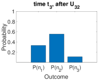
Figure 6: Validating the predictions of weak macroscopic realism: The sequence as Alice makes the operations $U_{f}$ on the states (top) $|\psi_{sup}\rangle$ and (lower) $\rho_{3,mix}$, which is the state after Bob’s measurement detects the system in state $|3\rangle$ at time $t_{2}$. Alice first transforms (shuffling between boxes 1 and 2) according to $U_{f2}^{-1}=U_{21}$, leaving Box 3 untouched. Then she transforms (shuffling between boxes 3 and 2) by $U_{1f}^{-1}=U_{32}$. Far left are the plots of $P(n_{k})$ for the initial states (top) $|\psi_{sup}\rangle$ and (lower) $\rho_{mix}$. Second from left are the states after Alice’s transformation $U_{21}$. The predictions for the $|\psi_{sup}\rangle$ and the mixture $\rho_{3,mix}$ are identical. Far right are the states after Alice’s transformation (shuffling between boxes 2 and 3) $U_{32}$, where the predictions diverge. The results are in agreement with the predictions of weak macroscopic realism, which posits that the system has a definite property $\lambda_{3}$ for Box 3 (the ball is in the box or not) at time $t_{2}$, and this property cannot be changed by any shuffling $U_{21}$ on boxes 2 and 1. This is because throughout the shuffling $U_{21}$, the predictions are identical to those of the mixture $\rho_{3,mix}$, which is consistent with the definite value $\lambda_{3}$.

We now confirm that the predictions of the quantum paradox are indeed consistent with this hypothesis. We see that $U_{2f}=U_{2i}$. Hence, the state after this transformation is

$$U_{2f}^{-1}|\psi_{sup}\rangle = \frac{1}{\sqrt{2}}\left(\begin{array}[]{ccc}ie^{-i\varphi_{1}}&e^{-i\varphi_{1}}&0\\ -ie^{-i\varphi_{1}}&e^{-i\varphi_{1}}&0\\ 0&0&\sqrt{2}\end{array}\right)\frac{e^{-i\varphi}}{\sqrt{3}}\left(\begin{array}[]{c}-e^{i\varphi_{1}}\\ ie^{i\varphi_{1}}\\ 1\end{array}\right)$$ (101)

$$= \frac{e^{-i\varphi}}{\sqrt{6}}\left(\begin{array}[]{c}0\\ 2i\\ \sqrt{2}\end{array}\right)$$ (105)

which gives relative probabilities of $0$, $2/3$ and $1/3$, for detection of the system in the states $|1\rangle$, $|2\rangle$ and $|3\rangle$. We next compare the evolution under $U_{2f}^{-1}$ for the mixed state

$$\rho_{3,mix} = \frac{1}{3}(ie^{i\varphi_{1}}|2\rangle-e^{i\varphi_{1}}|1\rangle)(-ie^{-i\varphi_{1}}\langle 2|-e^{-i\varphi_{1}}\langle 1|)$$ (106)

$$+\frac{1}{3}|3\rangle\langle 3|$$

The system in a mixed state can be viewed as being in a state with a definite outcome for $\hat{n}$ on the mode $3$. Hence, there is a hidden variable $\lambda_{3}$ for the system in this description. Beginning with $\rho_{3,mix}$, the state after the transformation $U_{2f}^{-1}$ is

$$\rho_{3,mix,I} = \frac{2}{3}|2\rangle\langle 2|+\frac{1}{3}|3\rangle\langle 3|$$ (107)

which has identical relative probabilities of $0$, $2/3$ and $1/3$. There is consistency with wMR for mode $3$.

On the other hand, if we continue to evolve with $U_{1f}^{-1}$, then the evolution of the two states $|\psi_{sup}\rangle$ and $\rho_{3,mix}$ diverges macroscopically. For $|\psi_{sup}\rangle$, we find

$$U_{1f}^{\dagger}U_{2f}^{\dagger} = \frac{1}{\sqrt{3}}\left(\begin{array}[]{ccc}\sqrt{3}&0&0\\ 0&ie^{-i\varphi}&-e^{-i\varphi}\sqrt{2}\\ 0&-ie^{-i\varphi}\sqrt{2}&-e^{-i\varphi}\end{array}\right)\frac{e^{-i\varphi}}{\sqrt{6}}\left(\begin{array}[]{c}0\\ 2i\\ \sqrt{2}\end{array}\right)$$ (114)

$$= \frac{e^{-i\varphi}}{\sqrt{18}}\left(\begin{array}[]{c}0\\ -4e^{-i\varphi}\\ \sqrt{2}e^{-i\varphi}\end{array}\right)$$ (118)

There is zero probability of finding the system in state $|1\rangle$. The relative probabilities are $0$, $8/9$, $1/9$. On the other hand, for the system initially in $\rho_{3,mix}$, the final state after both the transformations $U_{2f}^{-1}$ and then $U_{1f}^{-1}$ is

$$\rho_{3,mix,F}=\frac{2}{3}U_{1f}^{-1}|2\rangle\langle 2|U_{1f}+\frac{1}{3}U_{1f}^{-1}|1\rangle\langle 1|U_{1f}$$ (119)

where

$$U_{1f}^{-1}|2\rangle=\frac{e^{-i\varphi}}{\sqrt{3}}\left(\begin{array}[]{c}0\\ i\\ -i\sqrt{2}\end{array}\right)$$ (120)

and

$$U_{1f}^{-1}|1\rangle=\left(\begin{array}[]{c}1\\ 0\\ 0\end{array}\right)$$ (121)

The probability of finding the system in state $|1\rangle$ is $1/3$. The evolution of $|\psi_{sup}\rangle$ leads to the paradox, but does not contradict the premise of weak macroscopic realism, because the local unitary transformation $U_{32}$ acts on both mode $3$ and $2$. The transformations are depicted in Figure 6.

The paradox is seen to arise from the distinction between the state before and after Bob’s measurement, which is initially microscopic. This gives the seemingly paradoxical situation whereby the measurement disturbance from Bob vanishes, but the effect of it nonetheless can be extracted by suitable dynamics.

V Macroscopic three-box paradox with cat states

The example of Sections III and IV considered states distinct by $N$ quanta. However, the calculations involved the interaction $H_{kl}$, which was solved for $N\sim 10$. One way to achieve a more macroscopic realisation of the three-box paradox is to consider the coherent states $|\alpha\rangle$ of a single-mode field. In this section, we propose such a paradox, where the separation between the relevant coherent states can be made arbitrarily large. In order to achieve a feasible realisation, the macroscopic paradox is based on a modified version of the original three-box paradox.

Superpositions of macroscopically distinct coherent sates are referred to as “cat states” s-cat ; cat-states ; cat-states-review ; yurke-stoler-1 . Such states can be generated in optical cavities with dissipation and /or using conditional measurements cat-states ; cat-det-map ; cat-state-phil ; collapse-revival-super-circuit-1 ; cat-states-super-cond ; cat-bell-wang-1 ; cat-states-wc ; transient-cat-states-leo ; cats-hach ; cat-even-odd-transient ; cat-dynamics-ry ; IBM-macrorealism-1 ; omran-cats . Here, we take a simple model in which the cat states are created from a nonlinear dispersive medium, where losses are assumed minimal yurke-stoler-1 ; wright-walls-gar-1 . The unitary operations are solved analytically, and have been realised experimentally, to create cat states for large $\alpha$ collapse-revival-super-circuit-1 ; collapse-revival-bec-2 .

V.1 Coherent-state model: $k>2$

We propose four states defined as

$$|1\rangle = |-i\alpha_{0}\rangle$$

$$|2\rangle = |i\alpha_{0}\rangle$$

$$|3\rangle = |\alpha_{0}\rangle$$

$$|4\rangle = |-\alpha_{0}\rangle$$ (122)

where $|\alpha\rangle$ is a coherent state of a single-mode field. As $\alpha_{0}\rightarrow\infty$, these states become orthogonal. We note that for sufficiently large $\alpha_{0}$, the states can be distinguished by simultaneous quadrature phase amplitude measurements $\hat{X}=\hat{a}+\hat{a}^{\dagger}$ and $\hat{P}=(\hat{a}-\hat{a}^{\dagger})/i$, where $\hat{a}$ and $\hat{a}^{\dagger}$ are the field boson destruction and creation operators yurke-stoler-1 .

The system can be prepared at time $t_{1}$ from the state $|3\rangle$ in the superposition yurke-stoler-1 ; manushan-cat-lg of type Eq. (1), by applying a set of unitary transformations based on nonlinear interactions. Following the work of Yurke and Stoler yurke-stoler-1 , we consider the evolution of a single mode system prepared in a coherent state under the influence of a nonlinear Hamiltonian written in the Schrödinger picture as,

$$H_{NL}=\omega\hat{n}+\Omega\hat{n}^{k}$$ (123)

where $\varOmega$ represents the strength of the nonlinear term and $\hat{n}=\hat{a}^{\dagger}\hat{a}$ is the field number operator. We take $\hbar=1$. Here, $k$ is a positive integer. After an interaction time of $t=\frac{\pi}{2\Omega}$, the system with $k>2$ initially prepared in a coherent state $|\alpha\rangle$ becomes

$$|\psi_{sup}\rangle = \frac{1}{2}(|1\rangle-|2\rangle+|3\rangle+|4\rangle)$$ (124)

$$= \frac{1}{2}(|-i\alpha_{0}\rangle-|i\alpha_{0}\rangle+|\alpha_{0}\rangle+|-\alpha_{0}\rangle)$$

which for large $\alpha_{0}$ is a a four-component cat state. Since it is produced at time $t_{1}$, we also refer to the state $|\psi_{sup}\rangle$ as $|\psi_{1}\rangle$. We can interpret the creation of the state as a transformation using a unitary operator $U_{i}=U_{\left(\frac{\pi}{2\Omega}\right)}$ given by

$$U_{i}|3\rangle=U_{i}|\alpha_{0}\rangle=|\psi_{sup}\rangle$$ (125)

where $U_{\left(\frac{\pi}{2\Omega}\right)}=e^{-i\Omega\hat{n}^{k}t}$ with $\hbar=1$. For large $\alpha_{0}$ where the four states can form a basis set $\{|1\rangle,$ $|2\rangle$, $|3\rangle$, $|4\rangle$}, it is convenient to identify the transformation as a matrix

$$U_{i} = \frac{1}{2}\left(\begin{array}[]{cccc}1&1&1&-1\\ 1&1&-1&1\\ -1&1&1&1\\ 1&-1&1&1\end{array}\right)$$ (130)

where the basis states $|k\rangle$ correspond to column matrices $(a_{j1})$ with coefficients given as $a_{j1}=\delta_{jk}$. It is straightforward to verify that the operations $U_{i}|k\rangle$ realise the correct final states.

To account for the four states, we consider a modified version of the three-box paradox. Bob can consider to determine whether the system is in one of the four states $|k\rangle$, analogous to four boxes. The initial state $|\psi_{sup}\rangle\equiv|\psi_{1}\rangle$ which Bob makes a measurement on is $|1\rangle-|2\rangle+|3\rangle+|4\rangle$. Bob may make measurements to determine whether the system is in one of the states $|2\rangle$ or $|4\rangle$, or not. If the system can be determined to be in neither $|2\rangle$ nor $|4\rangle$, then the reduced state for the system is $|1\rangle+|3\rangle$. Alternatively, Bob may make measurements to determine whether the system is in one of the states $|1\rangle$ or $|4\rangle$, or not. If the system is determined to be in neither $|1\rangle$ or $|4\rangle$, then the reduced state for the system is $-|2\rangle+|3\rangle$.

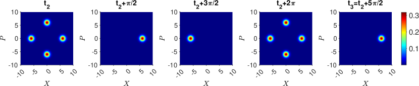
Figure 7: Dynamics of Alice’s transformation $U_{f}$ performed on the system in state $|\psi_{f}\rangle=-|1\rangle+|2\rangle+|3\rangle+|4\rangle$ at time $t_{2}$. The operation $U_{f1}$ is carried out by evolving under $H_{NL}$ for a time $t=3\pi/2\Omega$. Next, the operation $U_{f2}$ is carried out by evolving under $H_{NL}$ for a further time $t=\pi/\Omega$. At time $t_{3}$ after the combined operation $U_{f}=U_{f2}U_{f1}$, the system is in state $|3\rangle$.

Suppose Alice postselects for the state

$$|\psi_{f}\rangle = -|1\rangle+|2\rangle+|3\rangle+|4\rangle$$ (131)

$$= \frac{1}{2}(|\alpha_{0}\rangle+|-\alpha_{0}\rangle-|-i\alpha_{0}\rangle+|i\alpha_{0}\rangle))$$ (132)

which is generated from $|\alpha_{0}\rangle=|3\rangle$ by a transformation

$$U_{f}^{-1}|3\rangle=|\psi_{f}\rangle$$ (133)

The dynamics for $U_{f}$ is shown in Figure 7. The inverse is done by first transforming $|\alpha_{0}\rangle\rightarrow$$|-\alpha_{0}\rangle$, using the nonlinear interaction modelled by the Hamiltonian $H_{NL}$ of Eq. (123). Defining $U_{f2}=U_{\left(\frac{\pi}{\Omega}\right)}=e^{-i\Omega\hat{n}^{k}t}$ where the interaction time is $t=\pi/\Omega$, the state $|\alpha_{0}\rangle$ becomes $|-\alpha_{0}\rangle$, for all integers $k$. We identify

$$U_{f2}^{-1} = \left(\begin{array}[]{cccc}0&1&0&0\\ 1&0&0&0\\ 0&0&0&1\\ 0&0&1&0\end{array}\right)$$ (138)

and note that $U_{f2}^{-1}|\alpha_{0}\rangle=|-\alpha_{0}\rangle$. We also see that $U_{f2}^{-1}=U_{f2}$. The second stage of the generation is to transform $|4\rangle=|-\alpha_{0}\rangle$ by the unitary transformation $U_{f1}^{-1}$ so that

$$U_{f1}^{-1}|4\rangle=|\psi_{f}\rangle$$ (139)

We find that $U_{f1}^{-1}=U_{\left(\frac{\pi}{2\Omega}\right)}=e^{-i\Omega\hat{n}^{k}t}$ where $t=\pi/2\Omega$, and note that $U_{f1}^{-1}=U_{i}$. It is straightforward to verify that $U_{f1}^{-1}|4\rangle=|\psi_{f}\rangle$. In fact, $U_{f1}=U_{i}^{-1}$. Since for any unitary interaction $U=e^{-iHt}$, $U^{-1}=U^{\dagger}$, the inverse $U^{-1}$ corresponds to $U^{-1}=e^{iHt}$. Since the evolution is periodic, with period $2\pi/\Omega$ yurke-stoler-1 , this corresponds to $U^{-1}=e^{iH_{NL}(t-2\pi/\Omega)}=e^{-iH_{NL}(2\pi/\Omega-t)}$ and we find that $U_{f1}=U_{i}^{-1}=U_{\left(\frac{3\pi}{2\Omega}\right)}$. The $U_{f1}$ is realised by Alice evolving the system forward in time by the amount $t=3\pi/2\Omega$. We may express this as

$$U_{f1}^{-1}U_{f2}^{-1}|3\rangle=|\psi_{f}\rangle$$ (140)

which implies

$$U_{f}|\psi_{f}\rangle\equiv U_{f2}U_{f1}|\psi_{f}\rangle=|3\rangle$$ (141)

The operations $U_{f}$ correspond to Alice first evolving the system under $H$ with $k>2$ for a time $t=3\pi/2\Omega$, and then applying the evolution $H$ for a time $t=\pi/\Omega$. We find that $U_{f}=U_{f2}U_{f1}=U_{f2}^{-1}U_{i}^{-1}$: Hence, in matrix form

$$U_{f} = \frac{1}{2}\left(\begin{array}[]{cccc}1&1&1&-1\\ 1&1&-1&1\\ -1&1&1&1\\ 1&-1&1&1\end{array}\right)$$ (146)

Figure 7 shows the dynamics of Alice’s $U_{f}$, where the system is initially in the state $|\psi_{f}\rangle$. The evolution confirms that the final state is indeed $|3\rangle$.

The paradox is realised when Alice performs the measurement given by the transformation $U_{f}$ and detects whether the system is in state $|3\rangle$. We check for the paradox as follows. If Bob detects the system to be in $|2\rangle$, then the evolution by Alice gives

$$U_{f}|2\rangle = \frac{1}{2}\left(\begin{array}[]{c}1\\ 1\\ 1\\ -1\end{array}\right)$$ (151)

If Bob detects that the system is in state $|4\rangle$, then the evolution by Alice gives

$$U_{f}|4\rangle = \frac{1}{2}\left(\begin{array}[]{c}-1\\ 1\\ 1\\ 1\end{array}\right)$$ (156)

If Bob detects that the system is in state $|1\rangle$, then the evolution by Alice gives

$$U_{f}|1\rangle = \frac{1}{2}\left(\begin{array}[]{c}1\\ 1\\ -1\\ 1\end{array}\right)$$ (161)

If Bob detected that the system is not in $|2\rangle$ or $|4\rangle$, then the system is in reduced state $|1\rangle+|3\rangle$, and the evolution by Alice gives the final state

$$U_{f}(|1\rangle+|3\rangle)/\sqrt{2} = \frac{1}{\sqrt{2}}\left(\begin{array}[]{c}1\\ 0\\ 0\\ 1\end{array}\right)$$ (166)

If Bob detected that the system is not in $|1\rangle$ or $|4\rangle$, then the system is in reduced state $-|2\rangle+|3\rangle$, and the evolution by Alice gives the final state

$$U_{f}(-|2\rangle+|3\rangle)/\sqrt{2} = \frac{1}{\sqrt{2}}\left(\begin{array}[]{c}0\\ -1\\ 0\\ 1\end{array}\right)$$ (171)

In both cases, there is zero probability of Alice measuring the system to be in state $|3\rangle=|\alpha\rangle$. Hence, if Alice detects the system to be in $|\alpha_{0}\rangle$ at time $t_{3}$, she knows that Bob detected the ball to be in one of the boxes he opened. The dynamics is confirmed in Figures 8 and 9. The figures plot the dynamical sequences where Bob detects the Ball, and where Bob detects no Ball in Boxes 1 or 4. We confirm for the latter, there is zero probability of the system being found by Alice in state $|3\rangle.$

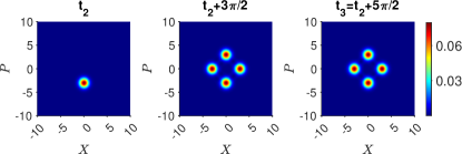
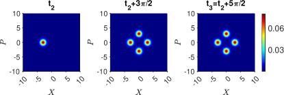
Figure 8: Dynamics of Alice’s transformation $U_{f}$ performed at time $t_{2}$ after Bob makes his measurement. Here, we take the case where Bob obtains the result: (top) that the Ball is in Box $1$ (implying the system is in state $|1\rangle$ at time $t_{2}$); or (lower) that the Ball is in Box 4 (implying the system is in state $|4\rangle$ at time $t_{2}$). The figures show contour plots of $Q(\alpha)$ for $\alpha_{0}=3$ and $k=3$. Here, $U_{f}=U_{f2}U_{f1}$. The plots show the state after the first transformation $U_{f1}$ at time $t_{2}+3\pi/2$. In both cases, there is a finite probability of Alice finding the Ball in Box $3$.

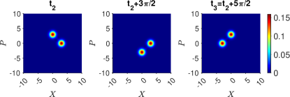
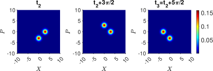
Figure 9: Dynamics of Alice’s transformation $U_{f}$ performed at time $t_{2}$ after Bob makes his measurement. Here, we take the case where Bob obtains the result: (top) that the Ball is not in Box 1 or 4 (implying the system in state $-|2\rangle+|3\rangle$ at time $t_{2}$); or (lower) that the Ball is not in Box 2 or 4 (so that the system in state $|1\rangle+|3\rangle$ at time $t_{2}$). The figures show contour plots of $Q(\alpha)$ for $\alpha_{0}=3$ and $k=3$. In both cases, there is zero probability of Alice finding the ball in Box 3.

The calculations can be summarised. If Bob opens Box 1 ($B1$) , then the probability of him detecting the ball is $1/4$. Following Maroney , we write this as $P_{B1}(1_{2})=1/4$. We see also that $P_{B1}(3_{3}|1_{2})=1/4$ and hence $P_{B1}(1_{2},3_{3})=P_{B1}(3_{3}|1_{2})P_{B1}(1_{2})=1/16$. Similarly, denoting the probability of detecting the ball in either Box 1 or 4 if both boxes are opened as $P_{B1,B4}(\{1_{2},4_{2}\})$, we find $P_{B1,B2}(\{1_{2},4_{2}\})=1/2$. From above, $P_{B1}(3_{3}|1_{2})=1/4$, and similarly, $P_{B1}(3_{3}|1_{2})=1/4$, but only one box can be detected with a ball. Hence, the probability of detecting a ball in Box 3 at time $t_{3}$, given Bob detected a ball in either Box 1 or 4 at time $t_{2}$, is $P_{B1,B4}(3_{3}|\{1_{2},4_{2}\})=1/4$. Hence

$$P_{B1,B4}(\{1_{2},4_{2}\},3_{3}) = P_{B1,B4}(3_{3}|\{1_{2},4_{2}\})$$ (172)

$$\times P_{B1,B4}(\{1_{2},4_{2}\})$$

$$= 1/8$$

The probability the ball is detected in Box 3, if Bob opens Boxes 1 and 4, is $P_{B1,B4}(3_{3})=\frac{1}{2}\{\frac{1}{4}\}+\frac{1}{2}\{0\}=1/8$. Hence, we obtain the key result:

$$P_{B1,B4}(\{1_{2},4_{2}\}|3_{3})=1$$ (173)

Similarly,

$$P_{B2,B4}(\{2_{2},4_{2}\}|3_{3})=1$$ (174)

We also note that

$$P_{B1,B4}(4_{2},3_{3}) = P_{B1,B4}(3_{3}|4_{2})P_{B1,B4}(4_{2})$$

$$= 1/16$$

which implies, since $P_{B1,B4}(3_{3})=1/8$,

$$P_{B1,B4}(4_{2}|3_{3})=1/2$$

Hence, Alice knows that, if she detects the ball in Box 3, the ball was detected in Box 4 only $50\%$ of the time. Yet, we see that the ball was detected with certainty in the set of boxes (either $1$ and $4$, or $2$ and $4$) that Bob opened. The paradox is that it seems as though for 50% of the time, the ball would be have to be detected in box 2 or 1, had that box been opened. The paradox is expressed as a violation of a Leggett-Garg inequality, in Section VI.

The effect of measurement disturbance is made apparent in this example. If Bob makes no measurement at time $t_{2}$, then the final state at time $t_{3}$ is $U_{f}|\psi_{sup}\rangle$:

$$U_{f}|\psi_{sup}\rangle = \left(\begin{array}[]{c}0\\ 0\\ 0\\ 1\end{array}\right)$$ (179)

There is zero probability that Alice detects a ball in Box 3: $P_{N}(3_{3})=0$. Yet, from the results above, if Bob opens Boxes 1 and 4, the probability of Alice observing the ball in Box 3 is $1/4$. Unlike the standard paradox, $P_{N}(3_{3})\neq P_{B1,B4}(3_{3})$. This means that Condition 1 of Ref. Maroney is not satisfied. We note however that the probability of Alice’s detecting a ball in Box 3, given Bob makes a measurement, is not affected by which pair of Boxes he opens: $P_{B1,B4}(3^{3})=1/4$ and $P_{B2,B4}(3^{3})=1/4$. This means part of Condition 1 of Maroney is satisfied. The transformation $U_{f}$, equivalent to a shuffle, does not give a relative enhancement of the probability of Alice detecting a Ball in Box 3 depending on which Boxes Bob opened.

V.2 Coherent-state model: $k=2$

The experimental realisation of $k>2$ may be challenging. However, the unitary interactions described in Yurke and Stoler have been experimentally verified for $k=2$ collapse-revival-super-circuit-1 ; collapse-revival-bec-2 . We can use

$$|1\rangle = |-i\alpha_{0}\rangle$$

$$|2\rangle = |i\alpha_{0}\rangle$$

$$|3\rangle = e^{-i\pi/4}|\alpha_{0}\rangle$$

$$|4\rangle = e^{-i\pi/4}|-\alpha_{0}\rangle$$ (180)

We consider

$$|\psi_{sup}\rangle\equiv|\psi_{1}\rangle=\frac{1}{2}\{|1\rangle+|2\rangle+|3\rangle-|4\rangle\}$$

This state yurke-stoler-1 ; manushan-cat-lg

$$\begin{array}[]{c}|\psi_{sup}\rangle=\frac{1}{2}\{|-i\alpha_{0}\rangle+|i\alpha_{0}\rangle+e^{-i\pi/4}|\alpha_{0}\rangle-e^{-i\pi/4}|-\alpha_{0}\rangle\}\\ \\ \end{array}$$ (181)

is formed at time $t=\pi/4\Omega$ from $|\alpha_{0}\rangle$, using the evolution given by $H_{NL}$ of Eq. (123) with $k=2$. We can interpret the creation of the state as a transformation using a unitary operator $U_{i}=U_{\left(\frac{\pi}{4\Omega}\right)}$ given by

$$U_{i}|3\rangle=U_{i}|\alpha_{0}\rangle=|\psi_{sup}\rangle$$ (182)

where $U_{\left(\frac{\pi}{4\Omega}\right)}=e^{\frac{-i\Omega\hat{n}^{k}t}{\hbar}}$ with $\hbar=1$.

Bob measures whether the system is in state $|1\rangle$ or $|4\rangle$, or not. If the system can be determined to be in neither $|1\rangle$ nor $|4\rangle$, then the reduced state for the system is $|2\rangle+|3\rangle$. Alternatively, Bob may make measurements to determine whether the system is in one of the states $|2\rangle$ or $|4\rangle$, or not. If the system is determined to be in neither $|2\rangle$ or $|4\rangle$, then the reduced state for the system is $|1\rangle+|3\rangle$.

Alice postselects for the state

$$|\psi_{f}\rangle = \frac{1}{2}\{|1\rangle+|2\rangle-|3\rangle+|4\rangle\}$$ (183)

$$= \frac{1}{2}\{|-i\alpha_{0}\rangle+|i\alpha_{0}\rangle$$

$$-e^{-i\pi/4}|\alpha_{0}\rangle+e^{-i\pi/4}|-\alpha_{0}\rangle\}$$

which is formed at time $t=\pi/4\Omega$ from $|-\alpha_{0}\rangle$, using $k=2$. We aim to find $U_{f}$ such that

$$U_{f}^{-1}|3\rangle=|\psi_{f}\rangle$$ (184)

As above, we first transform to $|4\rangle$. Defining $U_{f2}=U_{\left(\frac{\pi}{\Omega}\right)}=e^{\frac{-i\Omega\hat{n}^{k}t}{\hbar}}$ where the interaction time is $t=\pi/\Omega$, the state $|\alpha_{0}\rangle$ becomes $|-\alpha_{0}\rangle$, for $k=2$. We see that $U_{f2}=U_{f2}^{-1}$. We then apply

$$U_{f3}^{-1}U_{f2}^{-1}|3\rangle=|\psi_{f}\rangle$$ (185)

where we define $U_{f3}^{-1}=U_{\left(\frac{\pi}{4\Omega}\right)}=e^{-i\Omega\hat{n}^{k}t}$ with interaction time is $t=\pi/4\Omega$. We note that $U_{f3}=U_{\left(\frac{7\pi}{4\Omega}\right)}=e^{-i\Omega\hat{n}^{k}t}$ which corresponds to the interaction time $t=7\pi/4\Omega$. We find that $U_{f}=U_{f2}U_{f3}$.We find that $U_{f}=U_{f2}U_{f3}$.

Hence, Alice transforms the system according to $U_{f}$ and then detects whether the system is in state $|3\rangle$. The operations $U_{f}$ correspond to Alice first evolving the system under $H_{NL}$ with $k=2$ for a time $t=7\pi/4\Omega$, and then applying the evolution $H$ for a time $t=\pi/\Omega$. For the system in either $|2\rangle+|3\rangle$ or $|1\rangle+|3\rangle$ at time $t_{2}$, the probability for Alice obtaining a result $|3\rangle$ is zero, which leads to the paradox.

Realisation of the interactions $H_{NL}$ of Eq. (123) with $k=2$ have been achieved in the experiments of Kirchmair et al collapse-revival-super-circuit-1 . Bob’s projective measurements can be performed in principle by measuring the quadrature phase amplitude, along a chosen direction. For example, determining whether the system is in $|3\rangle$ or $|4\rangle$ can be determined by measuring $\hat{X}$. This will distinguish $|3\rangle$ and $|4\rangle$, but the outcome of zero gives no information about whether the system is in $|1\rangle$ or $|2\rangle$. Similarly, whether the system is in $|2\rangle$ or $|4\rangle$ (or $|1\rangle$ or $|4\rangle$) can be determined by measuring whether $\hat{X}_{\theta}$ is zero or not, for the right choice of rotated axis.

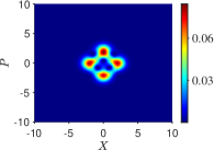
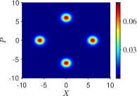
Figure 10: The $Q$ functions for the superposition $|\psi_{sup}\rangle$ (Eq. 124) (left) and the mixture $\rho_{mix,14}$ (Eq. 188) (right) become indistinguishable for large $\alpha_{0}$. The top and lower pairs are for $\alpha_{0}=2$ and $\alpha_{0}=6$ respectively.

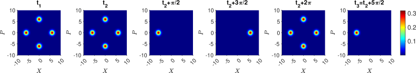
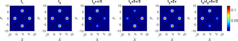
Figure 11: The dynamics of the macroscopic three-box paradox. The dynamics induced by Alice’s transformations $U_{f}$ is macroscopically sensitive to whether or not Bob has made a prior measurement on the system at time $t_{1}$, despite Bob’s measurement being seemingly non-invasive. The figure shows contour plots of $Q(\alpha)$ for the system prepared at time $t_{1}$ in the superposition state $|\psi_{sup}\rangle$ (Eq. (124)) (far left), as it evolves under the action of Bob and Alice’s operations. The top sequence shows the dynamics if there is no measurement made by Bob. Alice makes her transformation $U_{f}$ on the system starting at time $t_{2}$ (second from left). The dynamics of the transformation $U_{f}$ is completed at time $t_{3}$. The lower sequence shows the evolution if Bob makes a measurement on the system at time $t_{1}$ (the outcome revealing whether the system is in the state $|1\rangle$ or $|4\rangle$, or not). At time $t_{2}$, after Bob’s measurement, the system is in the mixed state $\rho_{mix,14}$. While the $Q$ function for $\rho_{mix,4}$ (lower second from left) is indistinguishable from that of $|\psi_{sup}\rangle$ (top second from left) as $\alpha\rightarrow\infty$, indicating a non-invasive measurement, there is a macroscopic difference between the final probabilities (top far right and lower far right) after the dynamics of Alice’s transformations, at time $t_{3}$. Here, $\alpha_{0}=6$ and $k=3$.

V.3 Consistency with macroscopic realism

We now analyse the dynamics of the three-box paradox for the macroscopic example using coherent states. The paradox can be modelled using the $Q$ function, defined by Husimi-Q-1

$$Q(\alpha)=\frac{\langle\alpha|\rho|\alpha\rangle}{\pi}$$ (186)

where $\rho$ is the system density operator. We examine the case of $k>2$. The case of $k=2$ will show similar behaviour. The system at time $t_{1}$ is in the superposition $|\psi_{sup}\rangle$ (Eq. (124)). The Q function is

$$Q(x,p) = e^{-\frac{(|\alpha|^{2}+|\alpha_{0}|^{2})}{2\pi}}\Bigr{(}2\cos\left(x\alpha_{0}-p\alpha_{0}\right)\sinh\left(x\alpha_{0}-p\alpha_{0}\right)$$ (187)

$$-2\cos\left(x\alpha_{0}+p\alpha_{0}\right)\sinh\left(x\alpha_{0}+p\alpha_{0}\right)$$

$$+\cosh\left(2x\alpha_{0}\right)+\cosh\left(2p\alpha_{0}\right)$$

$$+\cos\left(2p\alpha_{0}\right)-\cos\left(2x\alpha_{0}\right)\Bigl{)}$$

where $\alpha=x+ip$ and $\alpha_{0}$ is taken to be real. The function is depicted by the contour graph, in Figure 10.

Suppose Bob looks at Boxes 1 and 4. After the projective measurement by Bob to determine whether the system is in state $|1\rangle$ or $|4\rangle$, or not ($i=1,2$), the system is in the mixed state given by density operator

$$\rho_{mix,14}=\frac{1}{4}|1\rangle\langle 1|+\frac{1}{4}|4\rangle\langle 4|+\frac{1}{4}(-|2\rangle+|3\rangle)(-\langle 2|+\langle 3|)$$ (188)

The Q function of the mixed state created at time $t_{2}$ is

$$Q_{mix,14}(x,p) = e^{-\frac{(|\alpha|^{2}+|\alpha_{0}|^{2})}{2\pi}}\Bigr{(}\cosh\left(2x\alpha_{0}\right)+\cosh\left(2p\alpha_{0}\right)$$ (189)

$$-\exp\bigl{(}x\alpha_{0}+p\alpha_{0}\bigr{)}\cos\bigl{(}x\alpha_{0}+p\alpha_{0}\bigr{)}\Bigr{)}$$

plotted in Figure 10. Comparison of $Q(x,p)$ with $Q(x,p)_{mix,14}$ shows that as $\alpha_{0}\rightarrow\infty$, $Q(x,p)\rightarrow Q_{mix,14}(x,p)$. The terms contributing from the superposition are damped by a term exponential in $\alpha_{0}$.

Now Alice performs the transformations. The system evolves according to $U_{f}$. The final state if Bob made no measurement is given by Eq. (179), since the system remains in the superposition $|\psi_{sup}\rangle$ (Figure 11). On the other hand, the result if Bob opened Boxes 1 and 4 is different. The system is $\rho_{mix,14}$ at time $t_{2}$. After the transformations $U_{f}$, the system is in the mixed state

$$\rho_{mix,14}(t_{3}) = \frac{1}{4}[U_{f}|1\rangle\langle 1|U_{f}^{\dagger}]+\frac{1}{4}[U_{f}|4\rangle\langle 4|U_{f}^{\dagger}]$$

$$+\frac{1}{2}U_{f}(\frac{-|2\rangle+|3\rangle}{\sqrt{2}})(\frac{-\langle 2|+\langle 3|}{\sqrt{2}})U_{f}^{\dagger}$$

The states $U_{f}|1\rangle$, $U_{f}|4\rangle$ and $U_{f}(-|2\rangle+|3\rangle)/\sqrt{2}$ are given by Eqs. (161), (156) and (171). Figure 11 shows the final state after Alice’s operations $U_{f}$, for the two initial states $|\psi_{sup}\rangle$ and $\rho_{mix,14}$ at time $t_{2}$. While the $Q$ functions are initially indistinguishable, after the $U_{f}$, a macroscopic difference between the final states emerges. This is consistent with a model in which weak macroscopic realism holds, but where there is measurement disturbance due to Bob’s interactions.

VI Leggett-Garg test of macrorealism

The Leggett-Garg inequality can be violated for systems which do not jointly satisfy the combined premise of macroscopic realism and no measurement-disturbance. Leggett and Garg considered a system which at three times $T_{1}<T_{2}<T_{3}$ can be found to be in one of two macroscopically distinguishable states. If macroscopic realism holds, then the system is at each time always in one or other of the states, and can be ascribed the variable $\lambda_{k}$ at time $T_{k}$, where $\lambda_{k}=\pm 1$. If noninvasive measurability holds, there is no disturbance from a measurement made on the system to determine the value of $\lambda_{k}$. In this case, macrorealism is said to hold, and inequalities follow.

The application of a Leggett-Garg test to the three-box paradox elucidates the origin of the paradox Maroney . Maroney derived new versions of the Leggett-Garg inequality that applied to the paradox. The Condition 1 by Bob ensures that

$$P_{N}(3_{3})=P_{B1}(3_{3})=P_{B2}(3_{3})$$ (191)

This means that Alice observes no change in the probability of her detecting a Ball in Box 3, due to whether Bob opens one of the Boxes or not. Maroney referred to Bob’s measurement, which satisfies this condition, as operationally nondisturbing. Maroney pointed out that this condition is satisfied in the three-box paradox, but has not been satisfied in other tests of Leggett-Garg inequalities. The condition gives a particularly strong test of macrorealism. Here, we illustrate that the mesoscopic paradox of Section IV will satisfy the strict Maroney-Leggett-Garg test of macrorealism, and that violation of a Leggett-Garg inequality is also possible for the macroscopic system of Section III.

Following Maroney, we let $\lambda_{k}=-1$ if the system is found in $|1\rangle$ or $|2\rangle$, and $\lambda_{k}=1$ if the system is found in Box 3. At time $T_{1}$, the ball is in Box 3, and $\lambda_{1}=1$. The premise of macrorealism implies the Leggett-Garg inequality $-1\leq Q\leq 3$, where

$$Q=\langle\lambda_{1}\lambda_{2}\rangle+\langle\lambda_{2}\lambda_{3}\rangle+\langle\lambda_{1}\lambda_{3}\rangle$$ (192)

Consideration that macrorealism holds leads to constraints on the relations between the probabilities. We summarise the work of Maroney, since this will apply directly to the mesoscopic example. Using the initial condition, we find that $Q=\langle\lambda_{2}\rangle+\langle\lambda_{3}\rangle+\langle\lambda_{2}\lambda_{3}\rangle$ where $\langle\lambda_{2}\rangle=-P(1_{2})-P(2_{2})+P(3_{2})=2P(3_{2})-1$, and

$\langle\lambda_{3}\rangle=2P(3_{3})-1$. Macrorealism posits the ball to be in one of the boxes, which implies

$$P(3_{2})=P(3_{2},1_{3})+P(3_{2},2_{3})+P(3_{2},3_{3})$$ (193)

and similarly,

$$P(3_{3})=P(1_{2},3_{3})+P(2_{2},3_{3})+P(3_{2},3_{3})$$ (194)

Macrorealism also implies relations between joint probabilities and marginals, for example

$$P(1_{2}+2_{2},1_{3}+2_{3}+3_{3}) = \sum_{I_{2}=1,2}\sum_{J_{3}=1,2,3}P(I_{2},J_{3})$$ (195)

$$= P(1_{2}+2_{2})$$

$$= 1-P(3_{2})$$

Hence, macrorealism implies

$$\langle\lambda_{2}\lambda_{3}\rangle = P(3_{2},3_{3})+P(2_{2},2_{3})+P(1_{2},1_{3})+P(1_{2},2_{3})$$ (196)

$$+P(2_{2},1_{3})-P(3_{2},1_{3})-P(3_{2},2_{3})$$

$${\color[rgb]{1,0,0}{\normalcolor-P(1_{2},3_{3})-P(2_{2},3_{3})}}$$

$$= P(3_{2},3_{3})-(P(3_{2})-P(3_{2},3_{3}))$$

$$-(P(3_{3})-P(3_{2},3_{3}))$$

$$+1-P(3_{2})-(P(3_{3})-P(3_{2},3_{3}))$$

This leads to

$$Q = 4P(3_{2},3_{3})-1$$ (197)

$$= 4(P(3_{3})-P(1_{2},3_{3})-P(2_{2},3_{3}))-1$$

$$= 4P(3_{3})(1-P(1_{2}|3_{3})-P(2_{2}|3_{3}))-1$$

Considering the paradox of Section III, the probability of Alice detecting a Ball in box 3 at time $T_{3}$, regardless of a measurement by Bob, is $1/9$. The joint probability $P(1_{2},3_{3})$ is measurable by Alice and Bob, and calculable as $P(1_{2})P(3_{3}|1_{2})$. Here, $P(1_{2})=1/3$ and $P(3_{3}|1_{2})=1/3$, from the earlier sections. Alternatively, $P(1_{2},3_{3})=P(3_{3})P(1_{2}|3_{3})=P(3_{3})=1/9$, since $P(1_{2}|3_{3})=1$. The results for $P(2_{2},3_{3})$ are identical, giving $Q=-13/9$, which is a violation of the Leggett-Garg inequality, implying a negation of macrorealism. The test can be performed using the mesoscopic version of Section III, since the predictions are identical to the original paradox.

The calculation of the prediction $P(3_{3}|1_{2})$ assumes the system at time $T_{2}$ after Bob’s measurement is $|1\rangle$ which is the eigenstate. We have seen how the $Q$ function for the superposition differs from that of a mixed state. Prior to Bob’s measurement, the system can be viewed to be in a state with a definite outcome for the detection of the ball in the box, but the “state” the system is in is not the corresponding eigenstate.

The Leggett-Garg test is also applicable to the macroscopic set-up proposed in Section IV. We we let $\lambda_{k}=-1$ if the system is found in $|1\rangle$ or $|4\rangle$, $|2\rangle$ or $|4\rangle$, and $\lambda_{k}=1$ if the system is found in Box 3. At time $T_{1}$, the ball is in Box 3, and $\lambda_{1}=1$. We find $\langle\lambda_{2}\rangle=2P(3_{2})-1$ and $\langle\lambda_{3}\rangle=2P(3_{3})-1$. To derive $\langle\lambda_{2}\lambda_{3}\rangle$, extending the logic to apply to four possible states is straightforward e.g. macrorealism implies

$$P(3_{2}) = P(3_{2},1_{3})+P(3_{2},2_{3})+P(3_{2},3_{3})+P(3_{2},4_{3})$$

This leads to the expression above, and

$$Q = 4P(3_{2},3_{3})-1$$

$$= 4(P(3_{3})-P(1_{2},3_{3})-P(2_{2},3_{3})-P(4_{2},3_{3}))-1$$

Now, we know that since the ball can only be in one box, $P(\{1_{2},4_{2}\},3_{3})=P(1_{2},3_{3})+P(4_{2},3_{3})$. Hence,

$$Q = 4(P(3_{3})-P(1_{2},3_{3})-P(2_{2},3_{3})-P(4_{2},3_{3}))-1$$ (200)

$$= 4(P(3_{3})-P(\{1_{2},4_{2}\},3_{3})-P(\{2_{2},4_{2}\},3_{3})$$

$$+P(4_{2},3_{3}))-1$$

$$= 4(P(3_{3})-P_{B1,B4}(\{1_{2},4_{2}\},3_{3})-P_{B2,B4}(\{2_{2},4_{2}\},3_{3})$$

$$+P_{B1,B4}(4_{2},3_{3}))-1$$

$$= 4P_{B1,B4}(3_{3})\{1-\{P(\{1_{2},4_{2}\}|3_{3})-P(\{2_{2},4_{2}\}|3_{3})$$

$$+P_{B4}(4_{2}|3_{3})\}-1$$

Using the solutions $P_{B1,B4}(3_{3})=P_{B1,B2}(3_{3})=1/8$, $P_{B4}(4_{2}|3_{3})=1/2$ and $P(1_{2},4_{2}|3_{3})=1$ and $P(2_{2},4_{2}|3_{3})=1$, we find $Q=-5/4$, giving a violation of the Leggett-Garg inequality and hence a negation of macrorealism.

VII Conclusion

This paper gives proposals for mesoscopic and macroscopic quantum three-box paradoxes. The unitary operations (shuffling) required for the three-box paradox are realised by nonlinear interactions which we model by specific Hamiltonians. The motivation for considering the macroscopic versions is to argue the case for realism: The paradox may be explained as a failure of realism, or else explained by measurement disturbance.

We show how macroscopic realism can be upheld consistently with the paradox. Macroscopic realism asserts that the system found to be in two macroscopically distinct states has a predetermined value for the outcome of a measurement that distinguishes those states. In order to achieve consistency with macroscopic realism, the definition of macroscopic realism is refined, so that it applies to the system created at the time $t_{i}$ after the unitary operations that determine the local measurement basis. Moreover, the predetermined value cannot be changed by any operations or measurements on spatially separated systems. We refer to this restricted definition as weak macroscopic realism (wMR). Weak macroscopic realism has been shown consistent with violations of macroscopic Bell inequalities manushan-bell-cat-lg .

Following Maroney Maroney , we have shown that the realisation of the paradox corresponds to a violation of a Leggett-Garg inequality. Hence, the combined assumptions of macroscopic realism and noninvasive measurability (“macrorealism”) are negated by the paradox. Our proposals however are macroscopic, and have the advantage that macrorealism is tested in the spirit of the Leggett-Garg paper legggarg , applying to a system where macroscopic realism can be genuinely applied. We illustrate how the Leggett-Garg inequality is violated, and yet macroscopic realism upheld, the violation occurring due to a failure of noninvasive measurability.

Further, in this paper we illustrate the paradoxical features of the measurement disturbance, by manipulating the parameter that determines the size of the system. The disturbance becomes minimal with increasing size, yet the probabilities after Alice’s unitary operations remain macroscopically distinguishable, depending on whether a measurement occurred or not. This effect is similar to a quantum revival. We expect the origin is non-classical, arising from future boundary conditions based on the Q function DrummondReid2020 .

The definition of macroscopic realism is required to be minimal. Macroscopic realism posits that there is a predetermined value for the outcome of the macroscopic measurement: This means that the ball is either in the Box, or not, prior to Alice or Bob opening the Box. However, it can be shown that if the system is viewed as being in a ’state’ with the predetermined outcome $+$ or $-$, then that ’state’ cannot be given as a quantum state $|\psi_{+}\rangle$ or $|\psi_{-}\rangle$, prior to measurement manushan-bell-cat-lg . This points to an inconsistency between wMR and (the standard interpretation of) quantum mechanics, as in Schrödinger’s argument s-cat . The acceptance of wMR as part of the explanation of the paradox may raise other open questions.

Finally, we consider the possibility of an experiment. The unitary dynamics required for the proposal with coherent states has been realised in experiments collapse-revival-super-circuit-1 . The mesoscopic system may be realised for $N=2$ using the Hong-Ou-Mandel effect. We note that similar mesoscopic interactions may also be realisable for moderate $N$, by applying the CNOT gates of the IBM computer IBM-macrorealism-1 .

References

- (1) Y. Aharonov and L. Vaidman, Y. Aharonov and L. Vaidman, Complete description of a quantum system at a given time, J. Phys. A: Math. Gen. 24 2315 (1991). J. Phys. A: Math. Gen. 24 2315 (1991).
- (2) Y. Aharonov, P. G. Bergmann & J. L. Lebowitz, Time Symmetry in the Quantum Process of Measurement, Phys. Rev. B 134, 1410 (1964).
- (3) K. A. Kirkpatrick, Classical three-box ’paradox’, Journal of Physics A 36, 4891 (2003).
- (4) M. S. Leifer & R. W. Spekkens, Logical Pre- and Post-Selection Paradoxes, Measurement-Disturbance and Contextuality, International Journal of Theoretical Physics 44 1977 (2005).
- (5) M. S. Leifer & R. W. Spekkens, Pre- and Post-Selection Paradoxes and Contextuality in Quantum Mechanics, Phys. Rev. Lett. 95, 200405 (2005).
- (6) J. Finkelstein, What is paradoxical about the "Three-box paradox"? ArXiv. /abs/quant-ph/0606218 (2006).
- (7) Tamar Ravon and Lev Vaidman, The three-box paradox revisited, J. Phys. A: Math. Theor. 40 2873 (2007).
- (8) K. A. Kirkpatrick, Reply to ’The three-box paradox revisited’ by T Ravon and L Vaidman, Journal of Physics A 40, 2883 (2007).
- (9) O. J. E. Maroney, Measurements, disturbance and the three-box paradox, Studies in History and Philosophy of Science Part B: Studies in History and Philosophy of Modern Physics, 58, 41 (2017).
- (10) R. E. Kastner, The Three-Box “Paradox” and Other Reasons to Reject the Counterfactual Usage of the ABL Rule, Foundations of Physics, 29, 851 (1999).
- (11) L. Vaidman, The Meaning of Elements of Reality and Quantum Counterfactuals: Reply to Kastner, Foundations of Physics 29, 865 (1999).
- (12) Yakir Aharonov, Eliahu Cohen, Ariel Landau & Avshalom C. Elitzur, The Case of the Disappearing (and Re-Appearing) Particle, Scientific Reports 7: 531 (2017).
- (13) Pawel Blasiak and Ewa Borsuk, Causal reappraisal of the quantum three-box paradox, Phys. Rev. A 105, 012207 (2021).
- (14) P. Kolenderski, U. Sinha, L. Youning, T. Zhao, M. Volpini, A. Cabello, et al. (2011). Playing the Aharon-Vaidman quantum game with a Young type photonic qutrit (2011). ArXiv e-print service, arXiv:1107.5828.
- (15) K. J. Resch, J. S. Lundeen, & A. M. Steinberg (2004). Experimental Realization of the Quantum Box Problem, Physics Letters A, 324, 125(2004).
- (16) R. E. George, L. Robledo, O. J. E. Maroney, M. S. Blok, H. Bernien, M. L. Markham, et al., Opening up three quantum boxes causes classically undetectable wavefunction collapse, Proceedings of the National Academy of Sciences, 110, 3777 (2013).
- (17) G. Kirchmair et al., Observation of the quantum state collapse and revival due to a single-photon Kerr effect, Nature 495, 205 (2013).
- (18) B. Vlastakis, G. Kirchmair, Z. Leghtas, S. E. Nigg, L. Frunzio, S. M. Girvin, M. Mirrahimi, M. H. Devoret, R. J. Schoelkopf, Deterministically encoding quantum information using 100-photon schrödinger cat states, Science 342, 607 (2013).
- (19) M. Thenabadu and M.D. Reid, Bipartite Leggett-Garg and macroscopic Bell inequality violations using cat states: distinguishing weak and deterministic macroscopic realism, Phys. Rev. A 105, 052207 (2022); arXiv:2012.14997 [quant-ph]; M. D. Reid and M Thenabadu, Weak versus deterministic macroscopic realism, arXiv:2101.09476 [quant-ph].
- (20) Jesse Fulton, Run Yan Teh, and M. D. Reid, Argument for the incompleteness of quantum mechanics based on macroscopic and contextual realism: GHZ and Bohm-EPR paradoxes with cat states, arXiv:2208.01225
- (21) R. Rushin Joseph, M. Thenabadu, C. Hatharasinghe, J. Fulton, R-Y Teh, P. D. Drummond and M. D. Reid, Wigner’s Friend paradoxes: consistency with weak-contextual and weak-macroscopic realism models, arXiv 2211.02877 [quant-ph].
- (22) E. Schrödinger, The Present Status of Quantum Mechanics, Die Naturwissenschaften. 23, 807 (1935).
- (23) A. Leggett and A. Garg, Quantum mechanics versus macroscopic realism: is the flux there when nobody looks?, Phys. Rev. Lett. 54, 857 (1985).
- (24) M. Thenabadu, G-L. Cheng, T. L. H. Pham, L. V. Drummond, L. Rosales-Zárate and M. D. Reid, Testing macroscopic local realism using local nonlinear dynamics and time settings, Phys. Rev. A 102, 022202 (2020).
- (25) M. Thenabadu and M. D. Reid, Leggett-Garg tests of macrorealism for dynamical cat states evolving in a nonlinear medium, Phys. Rev. A 99, 032125 (2019).
- (26) M. Thenabadu and M. D. Reid, Macroscopic delayed-choice and retrocausality: quantum eraser, Leggett-Garg and dimension witness tests with cat states, Phys. Rev. A 105, 062209 (2022).
- (27) J. P. Dowling, Quantum optical metrology –the lowdown on high-n00n states, Contemporary Physics 49, 125 (2008).
- (28) H. J. Lipkin, N. Meshkov, and A. J. Glick, Validity of many-body approximation methods for a solvable model: exact solutions and perturbation theory, Nucl. Phys. 62,188 (1965).
- (29) M. Steel and M. J. Collett, Quantum state of two trapped Bose-Einstein condensates with a Josephson coupling, Phys. Rev. A 57, 2920 (1998).
- (30) L. D. Carr, D. R. Dounas-Frazer, and M. A. Garcia-March, Dynamical realization of macroscopic superposition states of cold bosons in a tilted double well, Europhys. Lett. 90, 10005 (2010).
- (31) Florian Fröwis, Pavel Sekatski, Wolfgang Dür, Nicolas Gisin, and Nicolas Sangouard, Macroscopic quantum states: measures, fragility, and implementations, Rev. Mod. Phys. 90, 025004 (2018).
- (32) B. Yurke and D. Stoler, Generating quantum mechanical superpositions of macroscopically distinguishable states via amplitude dispersion, Phys. Rev. Lett. 57, 13 (1986).
- (33) S. Haroche, “Nobel Lecture: Controlling photons in a box and exploring the quantum to classical boundary”, Rev. Mod. Phys. 85, 1083 (2013). D. J. Wineland, “Nobel Lecture: Superposition, entanglement, and raising Schrödinger’s cat”, Rev. Mod. Phys. 85, 1103 (2013).
- (34) Zaki Leghtas, Gerhard Kirchmair, Brian Vlastakis, Michel H. Devoret, Robert J. Schoelkopf, and Mazyar Mirrahimi, Deterministic protocol for mapping a qubit to coherent state superpositions in a cavity. Phys. Rev. A 87, 042315 (2013).
- (35) A. Ourjoumtsev, H. Jeong, R. Tualle-Brouri, P. Grangier, Generation of optical ‘Schrödinger cats’ from photon number states, Nature 448,784 (2007).
- (36) C. Wang et al., A Schrödinger cat living in two boxes, Science 352, 1087 (2016).
- (37) M. Wolinsky, H. J. Carmichael, Quantum noise in the parametric oscillator: From squeezed states to coherent-state superpositions, Phys. Rev. Lett. 60,1836 (1988).
- (38) L. Krippner, W. J. Munro, M. D. Reid, Transient macroscopic quantum superposition states in degenerate parametric oscillation: Calculations in the large-quantum-noise limit using the positive p representation, Phys. Rev. A 50, 4330 (1994).
- (39) E. E. Hach III, C. C. Gerry, Generation of mixtures of Schrödinger-cat states from a competitive two-photon process, Phys. Rev. A 49, 490 (1994).
- (40) L. Gilles, B. M. Garraway, P. L. Knight, Generation of nonclassical light by dissipative two-photon processes, Phys. Rev. A 49, 2785 (1994).
- (41) R. Y. Teh, F.-X. Sun, R. Polkinghorne, Q. Y. He, Q. Gong, P. D. Drummond, M. D. Reid, Dynamics of transient cat states in degenerate parametric oscillation with and without nonlinear kerr interactions, Phys. Rev. A 101, 043807 (2020).
- (42) H.-Y. Ku, N. Lambert, F.-J. Chan, C. Emary, Y.-N. Chen, F. Nori, Experimental test of non-macrorealistic cat states in the cloud, npj Quantum Information 6, 98 (2020).
- (43) A. Omran, H. Levine, A. Keesling, G. Semeghini, T. T. Wang, S. Ebadi, H. Bernien, A. S. Zibrov, H. Pichler, S. Choi, et al., Generation and manipulation of Schrödinger cat states in Rydberg atom arrays, Science 365, 570 (2019).
- (44) E. Wright, D. Walls and J. Garrison, Collapses and Revivals of Bose-Einstein Condensates Formed in Small Atomic Samples, Phys. Rev. Lett. 77, 2158 (1996).
- (45) M. Greiner, O. Mandel, T. Hånsch and I. Bloch, Collapse and revival of the matter wave field of a Bose-Einstein condensate, Nature 419, 51 (2002).
- (46) Kôdi Husimi. Some Formal Properties of the Density Matrix, Proc. Phys. Math. Soc. Jpn. 22: 264 (1940).
- (47) P. D. Drummond and M. D. Reid, Retrocausal model of reality for quantum fields, Phys. Rev. Research 2, 033266 (2020); P. D. Drummond and M. D. Reid, Objective Quantum Fields, Retrocausality and Ontology, Entropy 23, 749 (2021).