Quantum tunneling in the real-time path integral by the Lefschetz thimble method

Abstract

Quantum tunneling is mostly discussed in the Euclidean path integral formalism using instantons. On the other hand, it is difficult to understand quantum tunneling based on the real-time path integral due to its oscillatory nature, which causes the notorious sign problem. We show that recent development of the Lefschetz thimble method enables us to investigate this issue numerically. In particular, we find that quantum tunneling occurs due to complex trajectories, which are actually observable experimentally by using the so-called weak measurement.

1 Introduction

Quantum tunneling has been mostly discussed in the imaginary-time path integral formalism using instantons [1, 2, 3], which enables us to investigate interesting phenomena such as the decay rate of a false vacuum in quantum field theory (QFT), bubble nucleation in first order phase transitions and domain wall fusions. The tunneling amplitude one obtains in this way is suppressed in general by $e^{-S_{0}/\hbar}$ with $S_{0}$ being the Euclidean action for the instanton configuration, which reveals its genuinely nonperturbative nature.

A natural question to ask here is how to describe quantum tunneling directly in the real-time path integral. This is motivated since, in reality, there are also contributions from classical motion over the barrier (c.f., sphalerons in QFT), which cannot be taken into account by instantons. Also the real-time path integral is needed to obtain the quantum state after tunneling and its subsequent time-evolution. However, a naive analytic continuation of instantons leads to singular complex trajectories [4]. We clarify this issue completely by explicit Monte Carlo calculations.

The main obstacle in performing first-principle calculations in the real-time path integral by using a Monte Carlo method is the severe sign problem, which occurs due to the integrand involving an oscillating factor $e^{iS[x(t)]}$, where the action $S[x(t)]\in{\mathbb{R}}$ depends on the path $x(t)$. In order to overcome this problem, we use the generalized Lefschetz thimble method (GTM) [5], which was developed along the earlier proposals [6, 7, 8].

Recently there have been further important developments of this method. First, an efficient algorithm to generate a new configuration was developed based on the Hybrid Monte Carlo algorithm (HMC), which is applied to the variables after the flow [6, 9] or before the flow [10]. The former has an advantage that the modulus of the Jacobian associated with the change of variables is included in the HMC procedure of generating a new configuration, whereas the latter has an advantage that the HMC procedure simplifies drastically without increasing the cost as far as one uses the backpropagation to calculate the HMC force. Second, the integration of the flow time within an appropriate range has been proposed [11] to overcome the multi-modality problem that occurs when there are contributions from multiple thimbles that are far separated from each other in the configuration space. Third, it has been realized that, when the system size becomes large, there is a problem that occurs in solving the anti-holomorphic gradient flow equation, which can be cured by optimizing the flow equation with a kernel acting on the drift term [12].

Here we apply the GTM to the real-time path integral for the transition amplitude in a simple quantum mechanical system, where the use of various new techniques mentioned above turns out to be crucial [13]. This, in particular, enables us to identify the relevant complex saddle points that contribute to the path integral from first principles, which was not possible before. By introducing a large enough momentum in the initial wave function, we find that the saddle point becomes close to real, which clearly indicates the transition to classical dynamics.

In fact, the complex trajectories can be probed [14, 15] by the ensemble average of the coordinate $x(t)$ at time $t$, which gives the “weak value” [16] of the Hermitian coordinate operator $\hat{x}$ evaluated at time $t$ with a post-selected final wave function. Note that this is actually a physical quantity that can be measured by experiments (“weak measurement”) at least in principle. We calculate this quantity by taking the ensemble average numerically and reproduce the result obtained by solving the Schrödinger equation, which confirms the validity of our calculations.

The rest of this article is organized as follows. In section 2 we briefly review some previous works in the case of a double-well potential, which will be important in our analysis. In section 3 we explain the details of the calculation method used in applying the GTM to the real-time path integral. In section 4 we show our main result thus obtained. In particular, we identify relevant complex saddle points, which are responsible for quantum tunneling. Section 5 is devoted to a summary and discussions.

2 Brief review of previous works

In this section we review some previous works on a quantum system with a double-well potential

$$V(x)=\lambda(x^{2}-a^{2})^{2}\ ,$$ (1)

which is a typical example used to discuss quantum tunneling. Here we take $\lambda=1/2$ and $a=1$ in the potential (1). The Lagrangian is given by

$$L=\left(\frac{dx}{dt}\right)^{2}-(x^{2}-1)^{2}\ ,$$ (2)

up to an overall factor, where the mass is set to unity.

First we review Ref. [4], which discusses the analytic continuation of the instanton solution in the imaginary-time formalism. Then we review Ref. [17], in which all the solutions to the classical equation of motion were obtained analytically although it was not possible to identify the relevant complex solutions from the viewpoint of the Picard-Lefschetz theory.

2.1 Analytic continuation of the instanton

Here we discuss a complex classical solution that can be obtained by analytic continuation of the instanton solution in the imaginary-time formalism [4].

For that, we consider the Wick rotation $t=e^{-i\alpha}\tau$, where $\tau\in{\mathbb{R}}$ runs from $-\infty$ to $\infty$. In particular, $\alpha=0$ corresponds to the real time and $\alpha=\pi/2$ corresponds the imaginary time. The Lagrangian (2) becomes

$$L^{(\alpha)}=e^{2i\alpha}\left(\frac{dz}{d\tau}\right)^{2}-(z^{2}-1)^{2}\ ,$$ (3)

where $z(t)$ represents a complex path. For $\alpha=\frac{\pi}{2}$, we obtain a real solution

$$z^{\star}(\tau)=\tanh\tau\ ,$$ (4)

which satisfies the boundary condition

$$z^{\star}(-\infty)=-1\ ,\quad z^{\star}(\infty)=1$$ (5)

and therefore connects the two potential minima as we plot in Fig. 1 (Left). This is the instanton solution in the imaginary-time formalism, and it actually describes quantum tunneling as is discussed, for instance, in Ref. [1].

By making an analytic continuation from (4), we can obtain a solution for arbitrary $0<\alpha\leq\frac{\pi}{2}$, which is given by

$$z^{\star}(\tau)=\tanh\Big{(}i\tau e^{-i\alpha}\Big{)}$$ (6)

satisfying the same boundary condition (5). Note that this solution is complex for $\alpha<\frac{\pi}{2}$ and it gives a trajectory with a spiral shape as shown in Fig. 1 (Right) for $\alpha=0.1\times\frac{\pi}{2}$. For smaller and smaller $\alpha$, the trajectory winds more and more around the potential minima as $\tau\rightarrow\pm\infty$ and it also extends farther and farther in the complex plane. Thus the solution that can be obtained by analytic continuation from the instanton is actually singular in the $\alpha\rightarrow 0$ limit.

Figure 1: (Left) The instanton solution (4) in the imaginary time formalism ($\alpha=\frac{\pi}{2}$), which connects the two potential minima indicated by the horizontal dashed line. (Right) The trajectory of the complex solution obtained by analytic continuation from the instanton solution is shown in the complex plane for $\alpha=0.1\times\frac{\pi}{2}$.

On the other hand, if one plugs (6) in the action $S=\int dtL=e^{-i\alpha}\int d\tau L^{(\alpha)}$, one finds that the $\tau$ integration for different $\alpha$ is related to each other by just rotating the integration contour of $\tau$ in the complex plane, which implies that the action is independent of $\alpha$ due to Cauchy’s theorem. Therefore, the amplitude one obtains for this solution in the $\alpha\rightarrow 0$ limit is suppressed by $e^{iS[z^{\star}]/\hbar}=e^{-S_{\rm E}/\hbar}$, where $S_{\rm E}>0$ is the Euclidean action for the instanton solution (4), which implies that the amplitude can be correctly reproduced by the complex saddle point obtained in this way as far as one introduces an infinitesimal $\alpha>0$ as a kind of regulator.

2.2 Exact classical solutions for a double-well potential

From the Lagrangian (2), one can derive the complex version of the energy conservation

$$\left(\frac{dz}{dt}\right)^{2}+(z^{2}-1)^{2}=q^{2}\ ,$$ (7)

where $q$ is some complex constant. This differential equation can be readily solved as

$$z(t)=\sqrt{\frac{q^{2}-1}{2q}}\,\text{sd}\left(\sqrt{2q}(t+c),\sqrt{\frac{1+q}{2q}}\right)\ ,$$ (8)

where $c$ is another complex constant and $\text{sd}(x,k)$ is the Jacobi elliptic function. Thus the general classical solution can be parametrized by the two integration constants $q$ and $c$.

Let us fix the end points of the solution to be $z(0)=x_{\text{i}}$ and $z(T)=x_{\text{f}}$, which can be complex in general. Then one finds that the parameter $k=\sqrt{(1+q)/2q}$, which is called the elliptic modulus, must satisfy the condition [17]

$$n\omega_{1}(k)+m\omega_{3}(k)$$

$$=\frac{T}{2}+\sqrt{\frac{2k^{2}-1}{8}}\left[\text{sd}^{-1}\left(\frac{\sqrt{2k^{2}-1}}{k\sqrt{2-2k^{2}}}x_{\text{i}},k\right)-(-)^{n+m}\text{sd}^{-1}\left(\frac{\sqrt{2k^{2}-1}}{k\sqrt{2-2k^{2}}}x_{\text{f}},k\right)\right]$$ (9)

with $\omega_{1}(k)$ and $\omega_{3}(k)$ defined by

$$\omega_{1}(k) =K(k)\sqrt{k^{2}-\frac{1}{2}}\ ,$$ (10)

$$\omega_{3}(k) =iK\left(\sqrt{1-k^{2}}\right)\sqrt{k^{2}-\frac{1}{2}}\ ,$$ (11)

where $K(k)$ is the complete elliptic integral of the first kind. Note that the solution after fixing the end points still depends on two integers $(n,m)$, which we will refer to as modes of the solution in what follows. Once we have $k$ and hence $q=1/(2k^{2}-1)$ for a given mode $(m,n)$, we can determine the complex parameter $c$ in (8) from $z(0)=x_{\text{i}}$.

For each solution $z(t)$ obtained above, we can obtain a solution $\tilde{z}(t)=az(a\sqrt{2\lambda}t)$ for arbitrary $\lambda$ and $a$ in (1) that satisfies the boundary conditions $\tilde{z}(0)=ax_{\text{i}}$ and $\tilde{z}(T)=ax_{\text{f}}$.

3 The calculation method used in this work

In this section we explain how to perform Monte Carlo calculations for the real-time path integral. First we briefly review the basic idea of the GTM to solve the sign problem. Then we review the idea of integrating the flow time to solve the multi-modality problem. Finally we explain the problem of the anti-holomorphic gradient flow that occurs in large systems, and discuss how to solve it by optimizing the gradient flow.

3.1 The basic idea of the GTM

In this section we give a brief review of the GTM, which is a promising method for solving the sign problem based on the Picard-Lefschetz theory. Here we consider a general model defined by the partition function and the observable

$$Z=\int d^{N}x\,e^{-S(x)}\ ,\quad\langle\mathcal{O}\rangle=\frac{1}{Z}\int d^{N}x\,\mathcal{O}(x)\,e^{-S(x)}\ ,$$ (12)

where $x=(x_{1},x_{1},\cdots,x_{N})\in{\mathbb{R}}^{N}$ and $d^{N}x=\prod_{n=1}^{N}dx_{n}$. The action $S(x)$ is a complex-valued holomorphic function of $x$, which makes (12) a highly oscillating multi-dimensional integral and hence causes the sign problem when the number $N$ of variables becomes large.

Let us first recall that the Picard-Lefschetz theory makes the oscillating integral well-defined by deforming the integration contour using the anti-holomorphic gradient flow equation

$$\frac{dz_{i}(\sigma)}{d\sigma}=\overline{\frac{\partial S(z(\sigma))}{\partial z_{i}}}$$ (13)

with the initial condition $z(0)=x\in\mathbb{R}^{N}$, where $\sigma$ plays the role of the deformation parameter. This flow equation defines a one-to-one map from $x=z(0)\in{\mathbb{R}}^{N}$ to $z=z(\tau)\in\mathcal{M}_{\tau}\in{\mathbb{C}}^{N}$. Due to Cauchy’s theorem, the partition function and the observable (12) can be rewritten as

$$Z=\int_{\mathcal{M}_{\tau}}d^{N}z\,e^{-S(z)}\ ,\quad\langle\mathcal{O}\rangle=\frac{1}{Z}\int_{\mathcal{M}_{\tau}}d^{N}z\,\mathcal{O}(z)\,e^{-S(x)}\ .$$ (14)

The important property of the anti-holomorphic gradient flow equation (13) is that

$$\frac{dS(z(\sigma))}{d\sigma}=\sum_{i}\frac{\partial S(z(\sigma))}{\partial z_{i}}\frac{dz_{i}(\sigma)}{d\sigma}=\sum_{i}\left|\frac{\partial S(z(\sigma))}{\partial z_{i}}\right|^{2}\geq 0\ ,$$ (15)

which means that the imaginary part of the effective action is constant along the flow, whereas the real part $S(z(\sigma))$ keeps on growing with $\sigma$ unless one reaches some saddle point $z=z^{\star}$ defined by

$$\frac{\partial S(z^{\star})}{\partial z_{i}} =0\ .$$ (16)

Thus, in the $\tau\rightarrow\infty$ limit, the manifold $\mathcal{M}_{\tau}$ is decomposed into the so-called Lefschetz thimbles, each of which is associated with some saddle point. The saddle points one obtains in this way are called “relevant” in the Picard-Lefschetz theory. In particular, the saddle points on the original integration contour are always relevant. Note also that there can be many saddle points that are not obtained by deforming the original contour in this way, which are called “irrelevant”.

In the $\tau\rightarrow\infty$ limit, ${\rm Im}\,S(z)$ becomes constant on each Lefschetz thimble due to the property (15) so that the sign problem is solved except for the one coming from the measure $d^{N}z$. In the GTM [5], the flow time $\tau\rightarrow\infty$ limit is not taken, which has a big advantage over the earlier proposals [6, 7, 8] with $\tau=\infty$, which require prior knowledge of the relevant saddle points.

The sign problem can still be ameliorated by choosing $\tau\sim\log N$, which makes the reweighting method work. However, the large flow time $\tau$ causes the multi-modality problem (or the ergodicity problem) since the transitions among different regions of $\mathcal{M}_{\tau}$ that flow into different thimbles in the $\tau\rightarrow\infty$ limit are highly suppressed during the simulation.

3.2 Integrating the flow time

In order to solve both the sign problem and the multi-modality problem, it was proposed [11] to integrate the flow time $\tau$ as

$$Z_{W}=\int_{\tau_{\rm min}}^{\tau_{\rm max}}d\tau\,e^{-W(\tau)}\int_{\mathcal{M}_{\tau}}d^{N}z\,e^{-S(z)}$$ (17)

with some weight $W(\tau)$, which is chosen to make the $\tau$-distribution roughly uniform in the region $[\tau_{\rm min},\tau_{\rm max}]$. The use of this idea is important in our work since we have to be able to sample all the saddle points and the associated thimbles that contribute to the path integral.

For an efficient sampling in (17), we use the Hybrid Monte Carlo algorithm [18], which updates the configuration by solving a fictitious classical Hamilton dynamics treating ${\rm Re}S(z)$ as the potential. When we apply this idea to (17), there are actually two options.

One option is to define a fictitious classical Hamilton dynamics for $(z,\tau)\in\mathcal{R}$ with $z\in\mathcal{M}_{\tau}$, where $\mathcal{R}$ is the “worldvolume” obtained by the foliation of $\mathcal{M}_{\tau}$ with $\tau\in[\tau_{\rm min},\tau_{\rm max}]$. While this option has an important advantage (See footnote 2.), one has to treat a system constrained on the worldvolume, which makes the algorithm quite complicated. Another problem is that the worldvolume is pinched if there is a saddle point on the original integration contour, which causes the ergodicity problem.

Here we adopt the other option, which is to rewrite (17) as

$$Z_{W}=\int_{\tau_{\rm min}}^{\tau_{\rm max}}d\tau\,e^{-W(\tau)}\int d^{N}x\,\det J(x,\tau)\,e^{-S(z(x,\tau))}\ ,$$ (18)

where $z(x,\tau)$ represents the configuration obtained after the flow starting from $x\in{\mathbb{R}}^{N}$ and

$$J_{ij}(x,\tau)=\frac{\partial z_{i}(x,\tau)}{\partial x_{j}}$$ (19)

is the Jacobi matrix associated with the change of variables. Then one can define a fictitious classical Hamilton dynamics for $(x,\tau)\in{\mathbb{R}}^{N}\times[\tau_{\rm min},\tau_{\rm max}]$. Here one only has to deal with an unconstrained system, which makes the algorithm simple. The disadvantage, however, is that the Jacobian $\det J(x,\tau)$ that appears in (18) has to be taken into account by reweighting, which causes the overlap problem when the modulus $|\det J(x,\tau)|$ fluctuates considerably during the simulation. In that case, only a small number of configurations with large $|\det J(x,\tau)|$ dominate the ensemble average and hence the statistics cannot be increased efficiently. It turns out that this problem does not occur in the simulations performed in this work if we optimize the flow equation as we describe in section 3.3. In all the simulations, we have chosen $\tau_{\rm min}=0.2$, which is small enough to solve the multi-modality problem, and $\tau_{\rm max}=4$, which is large enough to obtain typical trajectories close to the relevant saddle point. Note also that the sign problem is solved already at $\tau\sim 2$.

Once we generate the configurations $(x,\tau)$, we can calculate the expectation value $\langle\mathcal{O}\rangle$ by taking the ensemble average of $\mathcal{O}(z(x,\tau))$ with the reweighting factor

$$R(x,\tau)=\det J(x,\tau)\,e^{-i\,{\rm Im}S(z(x,\tau))}$$ (20)

using the configurations $(x,\tau)$ obtained for an appropriate range of $\tau$ [19].

In either option of the HMC algorithm, the most time-consuming part is the calculation of the Jacobian $\det J(x,\tau)$, which is needed only in the reweighting procedure. In order to calculate the Jacobi matrix $J(x,\tau)$, one has to solve the flow equation

$$\frac{\partial}{\partial\sigma}J_{ij}(\sigma)=\overline{H_{ik}(z(\sigma))\,J_{kj}(\sigma)}$$ (21)

with the initial condition $J(0)=\textbf{1}_{N}$, where we have defined the Hessian

$$H_{ij}(z) =\frac{\partial^{2}S(z)}{\partial z_{i}\partial z_{j}}\ .$$ (22)

3.3 Optimizing the flow equation

In this section we discuss a problem that occurs when we use the original flow equation (13) for a system with many variables such as the one studied below. We solve this problem by optimizing the flow equation, which actually has large freedom of choice if we are just to satisfy the property (15). Here we explain the basic idea and defer a detailed discussion to the forth-coming paper [12].

The problem with the original flow (13) can be readily seen by considering how its solution $z(x,\sigma)$ changes when the initial value $z(x,0)=x\in{\mathbb{R}}^{N}$ changes infinitesimally. Note that the displacement $\zeta_{i}(\sigma)\equiv z_{i}(x+\delta x,\sigma)-z_{i}(x,\sigma)$ for an infinitesimal $\delta x$ can be obtained as

$$\zeta_{i}(\sigma)=J_{ij}(\sigma)\,\delta x_{j}\ ,$$ (23)

where $J_{ij}(\sigma)$ is the Jacobi matrix at the flow time $\sigma$, which satisfies the flow equation (21). Thus we find that the displacement satisfies the flow equation

$$\frac{d\zeta_{i}(\sigma)}{d\sigma}=\overline{H_{ij}(z(\sigma))\,\zeta_{j}(\sigma)}$$ (24)

with the boundary condition $\zeta_{i}(0)=\delta x_{i}$, where $H_{ij}(z)$ is the Hessian defined by (22).

Let us consider the singular value decomposition (SVD) of the Hessian $H_{ij}(z(\sigma))$ given as

$$H(z(\sigma))=U^{\top}(\sigma)\,\Lambda(\sigma)\,U(\sigma)\ ,$$ (25)

where $U(\sigma)$ is a unitary matrix and $\Lambda={\rm diag}(\lambda_{1},\cdots,\lambda_{N})$ is a diagonal matrix with $\lambda_{1}\geq\cdots\geq\lambda_{N}\geq 0$. Plugging this in (21), we obtain

$$\frac{dJ(\sigma)}{d\sigma}=U(\sigma)^{\dagger}\,\Lambda(\sigma)\,\overline{U(\sigma)\,J(\sigma)}\ ,$$ (26)

and similarly for the displacement

$$\frac{d\zeta(\sigma)}{d\sigma}=U(\sigma)^{\dagger}\,\Lambda(\sigma)\,\overline{U(\sigma)\,\zeta(\sigma)}\ .$$ (27)

Roughly speaking, the magnitude of the displacement $\zeta(\sigma)$ grows exponentially with $\sigma$, and the growth rate is given by a weighted average of the singular values with a weight depending on $\delta x$. If the singular values have a hierarchy $\lambda_{1}\gg\lambda_{N}$, some modes grow much faster than the others. This causes a serious technical problem in solving the flow equation since it may easily diverge.

In order to solve this problem, we pay attention to the freedom in defining the flow equation. As we discussed in section 3.1, the important property of the flow equation (13) is (15). Let us therefore consider a generalized flow equation

$$\frac{dz_{i}(\sigma)}{d\sigma}=\mathcal{A}_{ij}(z(\sigma),\overline{z(\sigma)})\overline{\frac{\partial S(z(\sigma))}{\partial z_{j}}}\ .$$ (28)

Then the equation (15) becomes

$$\frac{dS(z(\sigma))}{d\sigma}=\sum_{i}\frac{\partial S(z(\sigma))}{\partial z_{i}}\frac{dz_{i}(\sigma)}{d\sigma}=\sum_{ij}\frac{\partial S(z(\sigma))}{\partial z_{i}}\mathcal{A}_{ij}(z(\sigma),\overline{z(\sigma)})\overline{\frac{\partial S(z(\sigma))}{\partial z_{j}}}\ .$$ (29)

For this to be positive semi-definite, the kernel $\mathcal{A}_{ij}(z,\bar{z})$ has only to be Hermitian positive, and it does not have to be holomorphic.

The flow of the Jacobi matrix becomes

$$\frac{\partial}{\partial\sigma}J_{ij}(\sigma)=\mathcal{A}_{ik}\overline{H_{kl}(z(\sigma))\,J_{lj}(\sigma)}+\left(\frac{\partial\mathcal{A}_{il}}{\partial z_{k}}J_{kj}(\sigma)+\frac{\partial\mathcal{A}_{il}}{\partial\bar{z}_{k}}\overline{J_{kj}(\sigma)}\right)\overline{\frac{\partial S(z(\sigma))}{\partial z_{l}}}\ .$$ (30)

From (30), we obtain the flow of the displacement as

$$\frac{\partial}{\partial\sigma}\zeta_{i}(\sigma)=\mathcal{A}_{ik}\overline{H_{kl}(z(\sigma))\,\zeta_{l}(\sigma)}+\left(\frac{\partial\mathcal{A}_{il}}{\partial z_{k}}\zeta_{k}(\sigma)+\frac{\partial\mathcal{A}_{il}}{\partial\bar{z}_{k}}\overline{\zeta_{k}(\sigma)}\right)\overline{\frac{\partial S(z(\sigma))}{\partial z_{l}}}\ .$$ (31)

Let us here assume that the first term is dominant in (31). Then plugging (25) in (31), we obtain

$$\frac{d\zeta(\sigma)}{d\sigma}\sim\mathcal{A}\,U(\sigma)^{\dagger}\,\Lambda(\sigma)\,\overline{U(\sigma)\,\zeta(\sigma)}\ .$$ (32)

Therefore, by choosing

$$\mathcal{A}=U(\sigma)^{\dagger}\,\Lambda^{-1}(\sigma)\,U(\sigma)\ ,$$ (33)

we obtain

$$\frac{d\zeta(\sigma)}{d\sigma}\sim U(\sigma)^{\dagger}\,\overline{U(\sigma)\,\zeta(\sigma)}\ ,$$ (34)

in which the problematic hierarchy of singular values $\lambda_{i}$ in (27) is completely eliminated. From this point of view, (33) seems to be the optimal choice for the “preconditioner” $\mathcal{A}$ in the generalized flow equation (28). Note also that, under a similar assumption, the flow of the Jacobi matrix changes from (26) to

$$\frac{\partial}{\partial\sigma}J(\sigma)\sim U(\sigma)^{\dagger}\,\overline{U(\sigma)\,J(\sigma)}\ .$$ (35)

Therefore, the use of the optimal flow equation reduces the overlap problem that occurs due to the large fluctuation of $|\det J|$ in our algorithm.

In order to implement this idea in the simulation, let us first note that (33) can be written as

$$\mathcal{A}(z(\sigma),\overline{z(\sigma)}) =\Big{\{}H^{\dagger}(z(\sigma))H(z(\sigma))\Big{\}}^{-1/2}=\Big{\{}\overline{H(z(\sigma))}H(z(\sigma))\Big{\}}^{-1/2}\ .$$ (36)

Here we use the rational approximation

$$x^{-1/2} \approx a_{0}+\sum_{q=1}^{Q}\frac{a_{q}}{x+b_{q}}\ ,$$ (37)

which can be made accurate for a wide range of $x$ with the real positive parameters $a_{q}$ and $b_{q}$ generated by the Remez algorithm. Thus we obtain

$$\mathcal{A}(z,\bar{z}) \approx a_{0}\,\textbf{1}_{N}+\sum_{q=1}^{Q}a_{q}\,\Big{\{}\overline{H(z)}H(z)+b_{q}\,\textbf{1}_{N}\Big{\}}^{-1}\ ,$$ (38)

which is much easier to handle on a computer than (33). In particular, the matrix inverse $(\bar{H}H+b_{q}\textbf{1}_{N})^{-1}$ does not have to be calculated explicitly since it only appears in the algorithm as a matrix that acts on a particular vector, which allows us to use an iterative method for solving a linear equation such as the conjugate gradient (CG) method. The factor of $Q$ in the computational cost can be avoided by the use of a multi-mass CG solver [21]. These techniques are well known in the so-called Rational HMC algorithm [22, 23], which is widely used in QCD with dynamical strange quarks [24] and supersymmetric theories such as the BFSS and IKKT matrix models (See Refs. [25, 26, 27], for example.).

4 Monte Carlo results obtained by the GTM

In this section we present our results obtained by Monte Carlo calculations based on the GTM. The path integral for the time-evolved wave function can be represented as

$$\Psi(x_{\rm f};T)=\int dx\,e^{-S_{\rm eff}(x)}\ ,$$ (39)

where $dx=\prod_{n=0}^{N-1}dx_{n}$. The effective action $S_{\rm eff}(x)$ is a function of $x=(x_{0},\cdots,x_{N-1})$ given by

$$S_{\rm eff}(x)=-\frac{i\epsilon}{\hbar}\sum_{n=0}^{N-1}\left\{\frac{1}{2}\,m\left(\frac{x_{n+1}-x_{n}}{\epsilon}\right)^{2}-\frac{V(x_{n+1})+V(x_{n})}{2}\right\}-\log\Psi(x_{0})\ ,$$ (40)

where $x_{N}=x_{\rm f}$ and the initial wave function is chosen as

$$\Psi(x)=\frac{1}{(2\pi)^{1/4}\sigma^{1/2}}\exp\left\{-\frac{1}{4\sigma^{2}}(x-b)^{2}+\frac{ipx}{\hbar}\right\}\ .$$ (41)

In all the simulations in this article, we set $m=1$, $\hbar=1$, and the total time to $T=2$, which is divided into $N=20$ intervals.

Here we consider the double-well potential (1) with $a=1$. The height of the potential at the local maximum $x=0$ is $V_{0}=\lambda$. We use $b=-1$ and $\sigma=0.3$ for the initial wave function (41) so that it is well localized around $x=-1$, which is one of the potential minima. We choose the end point $x_{\rm f}=1$ to be the other potential minimum.

In order to choose an appropriate value for $\lambda$ in the potential to probe quantum tunneling, we consider the probability

$$P=\sum_{E\geq V_{0}}|\langle E|\Psi\rangle|^{2}$$ (42)

of the initial quantum state having energy larger than the potential barrier $V_{0}$, where $|E\rangle$ represents the normalized energy eigenstate with the energy $E$. If we choose the momentum $p=0$ in the initial wave function (41), we obtain $P\sim 0.11$ for $\lambda=2.5$. We therefore use $\lambda=2.5$ in our calculation.

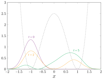
Figure 2: The distribution $|\Psi(x;t)|^{2}$ at time $t=0$ (purple line), $t=2$ (yellow line) and $t=5$ (green line) are shown for the initial wave function (41) with $\sigma=0.3$, $b=-1$, $p=0$ in the double-well potential (1) with $\lambda=2.5$, $a=1$ (gray, dashed line).

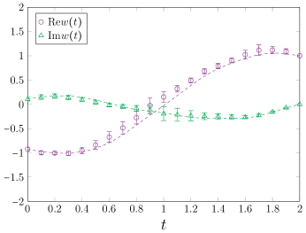
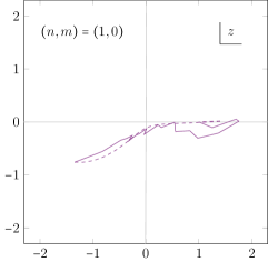
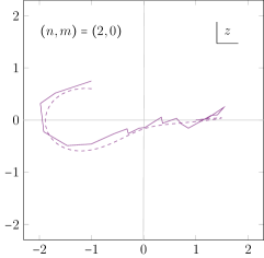
Figure 3: The results obtained for the initial wave function (41) with $\sigma=0.3$, $b=-1$, $p=0$ and $x_{\rm f}=1$ in the double-well potential (1) with $\lambda=2.5$, $a=1$. (Top) The weak value of the coordinate is plotted against time $t$ in the Left panel, while the trajectory of the weak value is plotted in the complex plane in the Right panel. The dashed lines represent the result obtained from (44) by solving the Schrödinger equation. (Bottom) Two typical trajectories obtained from the numerical simulation with the same parameters as in the Top panels. The dashed lines represent the closest classical solutions obtained by choosing the mode $(n,m)$ and the initial point $x_{\rm i}$ with the final point $x_{\rm f}=1$ fixed.

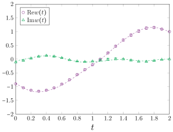
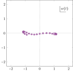
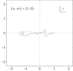
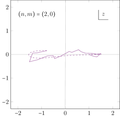
Figure 4: The results obtained for the initial wave function (41) with the momentum $p=-2$. All the other parameters are the same as in Fig. 3. (Top) The weak value of the coordinate is plotted against time $t$ in the Left panel, while the trajectory of the weak value is plotted in the complex plane in the Right panel. The dashed lines represent the result obtained from (44) by solving the Schrödinger equation. (Bottom) Two typical trajectories obtained from the numerical simulation with the same parameters as in the Top panels. The dashed lines represent the closest classical solutions obtained by choosing the mode $(n,m)$ and the initial point $x_{\rm i}$ with the final point $x_{\rm f}=1$ fixed.

Note that a typical tunneling time can be evaluated by

$$t_{0}\sim\frac{\pi\hbar}{\Delta E}\ ,$$ (43)

where $\Delta E$ is the energy difference between the ground state and the first excited state. For $\lambda=2.5$, we find $t_{0}\sim 5$. In Fig. 2 we plot the wave functions at $t=0$, $t=2$ and $t=5$ obtained for this setup by solving the Schrödinger equation with Hamiltonian diagonalization. The result for $t=2$ shows that the significant portion of the distribution has moved to the other potential minimum $x=1$, which implies that quantum tunneling has indeed occurred.

The expectation value of the coordinate $x(t)$ at time $t$ in the path integral (39) gives the weak value defined as [16]

$$w(t) =\frac{\langle x_{\rm f}|\,\hat{U}(T-t)\,\hat{x}\,\hat{U}(t)\,|\Psi\rangle}{\langle x_{\rm f}|\,\hat{U}(T)\,|\Psi\rangle}\ ,$$ (44)

where $\hat{U}(t)=\exp(-i\,t\hat{H}/\hbar)$ is the time-evolution unitary operator with the Hamiltonian $\hat{H}$. The quantum state $|\Psi\rangle$ corresponds to the initial wave function and $|x_{\rm f}\rangle$ represents the eigenstate of the coordinate operator. Note that the weak value is complex in general unlike the expectation value, which is real for a Hermitian operator such as $\hat{x}$. It is not only a mathematically well-defined quantity but also a physical quantity that can be measured by experiments using the so-called “weak measurement” [16]. Below we will see that the effects of the complex saddle points can be probed by the “weak value” of the coordinate operator $\hat{x}$ as pointed out in Refs. [14, 15].

In Fig. 3 (Top), we show our results for the weak value $w(t)$ of the coordinate at time $t$ defined by (44) for the initial wave function (41) with $\sigma=0.3$, $b=-1$, $p=0$ and $x_{\rm f}=1$ in the double-well potential (1) with $\lambda=2.5$, $a=1$. The dashed lines represent the results obtained directly from (44) by solving the Schrödinger equation with Hamiltonian diagonalization. The agreement between our data and the direct results confirms the validity of our calculation. We find that the weak value $w(t)$ is indeed complex except for the end point, which is fixed to $w(T)=x_{\rm f}=1$. Note that $w(0)$ is also complex although it is close to $x=-1$, which is the center of the Gaussian wave function (41).

In the Bottom panels of Fig. 3, we show two typical trajectories obtained from the simulation with the same parameters as in the Top panels. These trajectories are obtained for a relatively long flow time $\tau=4$ in the GTM (See section 3.2.) and therefore they are expected to be close to some relevant saddle points. Indeed we are able to find a classical solution discussed in section 2.2, which is close to each of these trajectories by choosing the mode $(n,m)$ and the initial point $x_{\rm i}$ with the final point $x_{\rm f}=1$ fixed. We find that the typical trajectories have a larger imaginary part on the left and a smaller imaginary part on the right, which suggests that quantum tunneling occurs first and then some classical motion follows. Note that this is different from the behaviors of the weak value $w(t)$ shown in the Top-Right panel. This is due to the fact that the weak value $w(t)$ is a weighted average of $x(t)$ obtained from the simulation, where the weight (20) is complex in general since it consists of the phase factor $e^{-i{\rm Im}S_{\rm eff}}$ and the Jacobian for the change of variables.

Next we introduce nonzero momentum $p=-2$ in the initial wave function (41). In Fig. 4 we show our results with all the other parameters the same as in Fig. 3. Since the initial kinetic energy is $p^{2}/2=2$, which is close to the potential barrier $\lambda=2.5$, a classical motion over the potential barrier is possible if the initial point $x(0)$ is slightly shifted from the potential minimum. Indeed we find that the weak value and the typical trajectories become close to real.

5 Summary and discussions

We have investigated quantum tunneling in the real-time path integral [13], which has important applications in QFT, quantum cosmology and so on. Unlike the previous works, we performed explicit Monte Carlo calculations based on the GTM. In particular, we were able to identify the complex trajectories that are relevant from the viewpoint of the Picard-Lefschetz theory. When we introduce momentum in the initial wave function, we found that the trajectories come closer to real, which clearly indicates the transition to classical dynamics.

In actual calculations, we integrate the flow time within an appropriate range to overcome the sign problem and the multi-modality problem [9]. We use the HMC algorithm on the real axis instead of using it on the deformed contour. This is made feasible by calculating the force using backpropagation [10]. Optimizing the flow equation [12] is also important. In particular, we do not observe the overlap problem due to reweighting $|{\rm det}J|$ in our calculations. We hope that our approach is useful in studying the real-time dynamics of various quantum systems.

Acknowledgements

We would like to thank Katsuta Sakai and Atis Yosprakob for collaborations [13, 12] that produced the results reported in this article. We are also grateful to Yuhma Asano and Masafumi Fukuma for valuable discussions. The computations were carried out on the PC clusters in KEK Computing Research Center and KEK Theory Center.

References

- [1] S. Coleman, Aspects of Symmetry: Selected Erice Lectures, Cambridge University Press (1985), 10.1017/CBO9780511565045.
- [2] S. Coleman, Fate of the false vacuum: Semiclassical theory, Phys. Rev. D 15 (1977) 2929.
- [3] C.G. Callan and S. Coleman, Fate of the false vacuum. ii. first quantum corrections, Phys. Rev. D 16 (1977) 1762.
- [4] A. Cherman and M. Unsal, Real-Time Feynman Path Integral Realization of Instantons, 1408.0012.
- [5] A. Alexandru, G. Basar, P.F. Bedaque, G.W. Ridgway and N.C. Warrington, Sign problem and monte carlo calculations beyond lefschetz thimbles, JHEP 05 (2016) 053 [1512.08764].
- [6] H. Fujii, D. Honda, M. Kato, Y. Kikukawa, S. Komatsu and T. Sano, Hybrid monte carlo on lefschetz thimbles - a study of the residual sign problem, JHEP 10 (2013) 147 [1309.4371].
- [7] AuroraScience collaboration, New approach to the sign problem in quantum field theories: High density qcd on a lefschetz thimble, Phys.Rev.D 86 (2012) 074506 [1205.3996].
- [8] E. Witten, Analytic continuation of Chern-Simons theory, AMS/IP Stud. Adv. Math. 50 (2011) 347 [1001.2933].
- [9] M. Fukuma, N. Matsumoto and N. Umeda, Implementation of the HMC algorithm on the tempered Lefschetz thimble method, 1912.13303.
- [10] G. Fujisawa, J. Nishimura, K. Sakai and A. Yosprakob, Backpropagating Hybrid Monte Carlo algorithm for fast Lefschetz thimble calculations, JHEP 04 (2022) 179 [2112.10519].
- [11] M. Fukuma and N. Matsumoto, Worldvolume approach to the tempered Lefschetz thimble method, PTEP 2021 (2021) 023B08 [2012.08468].
- [12] J. Nishimura, K. Sakai and A. Yosprakob, in preparation .
- [13] J. Nishimura, K. Sakai and A. Yosprakob, A new picture of quantum tunneling in the real-time path integral from Lefschetz thimble calculations, 2307.11199.
- [14] A. Tanaka, Semiclassical theory of weak values, Phys. Lett. A 297 (2002) 307 [quant-ph/0203149].
- [15] N. Turok, On Quantum Tunneling in Real Time, New J. Phys. 16 (2014) 063006 [1312.1772].
- [16] Y. Aharonov, D.Z. Albert and L. Vaidman, How the result of a measurement of a component of the spin of a spin-1/2 particle can turn out to be 100, Phys. Rev. Lett. 60 (1988) 1351.
- [17] Y. Tanizaki and T. Koike, Real-time Feynman path integral with Picard–Lefschetz theory and its applications to quantum tunneling, Annals Phys. 351 (2014) 250 [1406.2386].
- [18] S. Duane, A.D. Kennedy, B.J. Pendleton and D. Roweth, Hybrid Monte Carlo, Phys. Lett. B 195 (1987) 216.
- [19] M. Fukuma, N. Matsumoto and Y. Namekawa, Statistical analysis method for the worldvolume hybrid Monte Carlo algorithm, PTEP 2021 (2021) 123B02 [2107.06858].
- [20] J. Feldbrugge and N. Turok, Existence of real time quantum path integrals, Annals Phys. 454 (2023) 169315 [2207.12798].
- [21] B. Jegerlehner, Krylov space solvers for shifted linear systems, hep-lat/9612014.
- [22] A.D. Kennedy, I. Horvath and S. Sint, A New exact method for dynamical fermion computations with nonlocal actions, Nucl. Phys. B Proc. Suppl. 73 (1999) 834 [hep-lat/9809092].
- [23] M.A. Clark, The Rational Hybrid Monte Carlo Algorithm, PoS LAT2006 (2006) 004 [hep-lat/0610048].
- [24] M.A. Clark, A.D. Kennedy and Z. Sroczynski, Exact 2+1 flavour RHMC simulations, Nucl. Phys. B Proc. Suppl. 140 (2005) 835 [hep-lat/0409133].
- [25] S. Catterall and T. Wiseman, Towards lattice simulation of the gauge theory duals to black holes and hot strings, JHEP 12 (2007) 104 [0706.3518].
- [26] K.N. Anagnostopoulos, M. Hanada, J. Nishimura and S. Takeuchi, Monte Carlo studies of supersymmetric matrix quantum mechanics with sixteen supercharges at finite temperature, Phys. Rev. Lett. 100 (2008) 021601 [0707.4454].
- [27] S.-W. Kim, J. Nishimura and A. Tsuchiya, Expanding (3+1)-dimensional universe from a Lorentzian matrix model for superstring theory in (9+1)-dimensions, Phys. Rev. Lett. 108 (2012) 011601 [1108.1540].