Scalable quantum measurement error mitigation via conditional independence and transfer learning

Abstract

Mitigating measurement errors in quantum systems without relying on quantum error correction is of critical importance for the practical development of quantum technology. Deep learning-based quantum measurement error mitigation has exhibited advantages over the linear inversion method due to its capability to correct non-linear noise. However, scalability remains a challenge for both methods. In this study, we propose a scalable quantum measurement error mitigation method that leverages the conditional independence of distant qubits and incorporates transfer learning techniques. By leveraging the conditional independence assumption, we achieve an exponential reduction in the size of neural networks used for error mitigation. This enhancement also offers the benefit of reducing the number of training data needed for the machine learning model to successfully converge. Additionally, incorporating transfer learning provides a constant speedup. We validate the effectiveness of our approach through experiments conducted on IBM quantum devices with 7 and 13 qubits, demonstrating excellent error mitigation performance and highlighting the efficiency of our method.

I Introduction

Quantum computing offers computational advantages over classical algorithms across various problems, such as factoring integers, simulating quantum systems, solving linear systems of equations, machine learning, and simulating stochastic processes [1, 2, 3, 4, 5, 6, 7, 8, 9, 10]. However, the susceptibility of quantum computing to noise and imperfections poses a significant challenge, limiting its ability to surpass classical capabilities in solving real-world problems. While the theory of quantum error correction (QEC) and fault-tolerance holds the promise of scalable quantum computation [11, 12], building a fault-tolerant quantum computer remains a long-term endeavor. In the ongoing efforts to build full-fledged fault-tolerant quantum computers, there is a desire for techniques that improve the utility of quantum hardware in the presence of noise without relying solely on QEC.

Quantum error mitigation (QEM) refers to a set of techniques aimed at reducing the impact of errors on the outcomes of quantum computations [13, 14, 15, 16]. Unlike QEC, which completely removes errors, QEM focuses on minimizing their effects on the final result of an algorithm. By relaxing the requirement for full recovery of the desired state, QEM techniques can be implemented without the need for additional physical qubits. This makes QEM particularly well-suited for near-term quantum computing, where the size of quantum circuits that can be reliably executed is limited. In fact, QEM plays a crucial role in the Noisy Intermediate-Scale Quantum (NISQ) era [17], as it maximizes the utilization of limited quantum resources and expands the capacity of quantum systems for solving real-world problems [18, 19]. In this respect, developing the most efficient and scalable QEM techniques is an important task.

Measurement is an essential operation in quantum computing, but is prone to errors. In certain quantum devices, measurement errors can severely damage the overall computation. For instance, IBM quantum devices available on the cloud typically exhibit measurement error rates on the order of $1\%$, with some cases reaching as high as $40\%$. Various methods have been proposed to mitigate measurement errors [20, 21, 22, 23, 24], all of which are based on fully characterizing the underlying noise model using techniques such as tomography and machine learning. However, the computational costs associated with these methods scale exponentially with the number of qubits, imposing limitations on both scalability and practicality.

In this paper, we present a scalable deep learning-based method for quantum measurement error mitigation (QMEM). Our method leverages the concepts of conditional independence and transfer learning [25] to significantly improve the efficiency compared to previous methods. Conditional independence assumes that the impact of measurement cross-talk between distant qubits is negligible. This assumption is especially relevant for quantum devices with limited connectivity among physical qubits, such as those constrained by nearest-neighbor couplings [26] or employing distributed modular architectures [27, 28, 29, 30, 31]. By incorporating this assumption, we are able to exponentially reduce the size of neural networks used for QMEM. Transfer learning assumes the existence of an error component that is shared across all qubits. This assumption facilitates a constant factor reduction in training time by effectively leveraging pre-trained models. To validate our approach, we conducted proof-of-principle experiments on IBM quantum devices with 7 and 13 qubits. The results demonstrate that the underlying assumptions hold and affirm the effectiveness of our QMEM method in reducing measurement errors.

The remainder of the paper is organized as follows. We begin by setting up the problems and reviewing the two common approaches of QMEM in Section II. Section III presents the theoretical framework of our work, describing how the concept of conditional independence and transfer learning techniques are incorporated into the proposed QMEM method. In Section IV, we provide detailed instructions on how to implement the proposed QMEM methods and describe experiments conducted through the IBM quantum cloud service. This section also includes a comprehensive performance comparison between the proposed QMEM methods and existing methods. Conclusions are drawn in Section V, along with discussions on directions for future works and open problems.

II Background

Many experimental setups for both the quantum circuit model and quantum annealing use projective measurement in the computational basis to perform readout of a quantum state. Moreover, positive operator-valued measurements can be realized through the projective measurement with ancillary qubits [32, 33]. Therefore, our primary focus is the development of error mitigation techniques to enhance the projective measurement in the computational basis. An ideal measurement on $n$ qubits results in the probability distribution, which can be represented as a vector $\bm{p}=[p_{1},p_{2},...,p_{2^{n}}]$. However, the observed probability distribution in experiments deviate from $\bm{p}$ due to measurement errors. We denote the observed probability for each bitstring as $\hat{p}_{i}$ and the error map as $\mathcal{N}$ such that $\hat{\bm{p}}=\mathcal{N}(\bm{p})$. The goal of QMEM is to minimize the loss function, $D(\bm{p},\hat{\bm{p}})$ where $D$ is a distance measure that quantifies the discrepancy between the true and observed probability distributions.

The linear inversion method (LI-QMEM) assumes a noise model $\mathcal{N}(\bm{p})=\bm{\Lambda}\bm{p}$ and aims to reconstruct the noise matrix $\bm{\Lambda}$ through tomography. It produces an error-mitigated probability vector $\tilde{\bm{p}}=\bm{\Lambda}^{-1}\hat{\bm{p}}$ [20, 21, 22]. In contrast, QMEM can be performed by training a deep neural network $\mathcal{F}$ to approximate the inverse noise function $\mathcal{N}^{-1}$ [23, 24]. The trained neural network produces an error-mitigated probability vector $\tilde{\bm{p}}=\mathcal{F}(\hat{\bm{p}})\approx\mathcal{N}^{-1}(\hat{\bm{p}})=\bm{p}$. This approach, referred to as NN-QMEM, is capable of correcting non-linear errors, which is not possible with LI-QMEM [24]. However, both LI-QMEM and NN-QMEM suffer from scalability limitations as the memory and computation time grow exponentially with the number of qubits. Recent estimations suggest that the current classical computational resources can only handle NN-QMEM for quantum systems of up to 16 qubits [24]. This work focuses on overcoming the scalability limitation of NN-QMEM, since it can effectively correct non-linear errors.

III Theoretical Framework

III.1 Conditional Independence

Conditional independence (CI) is a fundamental concept in probability theory. It plays an important role in probabilistic models, simplifying the structure of the model and enabling an efficient analysis of the relationships between variables [34, 35]. It is valuable when modeling a large set of variables, where directly representing the joint distribution becomes challenging or impractical. By utilizing conditional independence relationships between variables, the joint distribution can be decomposed into smaller, more manageable components. This decomposition allows for a more tractable representation and analysis of complex probabilistic models. To illustrate this, consider the example of two random variables, $X$ and $Y$. We define $X$ and $Y$ as independent if and only if $p(X,Y)=p(X)p(Y)$. Independence between these variables leads to a partitioning of the probability distribution into two parts. For instance, if $X$ and $Y$ each take $2^{10}$ values, the full joint distribution $p(X,Y)$ would involve $2^{20}$ probabilities. Nevertheless, assuming independence between $X$ and $Y$ enables the decomposition of the joint distribution into the product of the individual distributions $p(X)$ and $p(Y)$. This decomposition significantly reduces the number of required probabilities to just $2^{10}+2^{10}=2^{11}$. Moreover, the definition of conditional independence is as follows. Let $X$, $Y$, and $Z$ be random variables. We say that $X$ and $Y$ are conditionally independent given $Z$ if the joint probability of $X$ and $Y$ given $Z$ can be expressed as $p(X,Y|Z)=p(X|Z)p(Y|Z)$. This indicates that the dependence between $X$ and $Y$ can be accounted for solely through their relationship with $Z$.

(a)

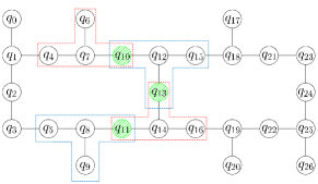
(b)

Figure 1: Layouts of the IBM quantum devices used in this work: (a) 7-qubit device and (b) 27-qubit device. Each circle labeled with $q_{i}$ represents the $i^{\mathrm{th}}$ physical qubit on the devices, while the connecting lines represent the qubit connectivity. In (b), we selected 13 qubits (from $q_{4}$ to $q_{16}$) for the experiment. The shaded yellow qubits indicate conditional qubits, and the qubits grouped within T-shaped boundaries represent subsystems with their respective conditional qubits (i.e., the leaf node and its parent in Fig. 2).

To understand how the concept of CI can be applied to QMEM, let us consider a 7 qubit system depicted in Fig. 1a, where $q_{i}$ denotes an $i^{\mathrm{th}}$ qubit. The circles and the wires in the figure represent physical qubits and their connectivity, respectively. The set of qubits $A=\{q_{0},q_{1},q_{2}\}$ and $B=\{q_{4},q_{5},q_{6}\}$ are connected only through $C=\{q_{3}\}$. Then assuming conditional independence of subsystems $A$ and $B$ given $C$, the joint probability distribution can be written as

$$p(A,B,C)=p(A,B|C)p(C)=p(A|C)p(B|C)p(C).$$

In the naive NN-QMEM, which aims to directly correct the full joint probability distribution $p(A,B,C)$, the number of input nodes of the neural network must grow exponentially with the number of qubits. Typically, the total number of nodes grows linearly with the number of input nodes, and the number of parameters grows quadratically. On the other hand, under the conditional independence assumptions, one needs three machine learning models that correct for $p(A|C)$, $p(B|C)$, and $p(C)$ independently. In this example, the number of input nodes for $p(A|C)$ and $p(B|C)$ is $2^{3}$, and is $2^{1}$ for $p(C)$. Since $C$ can take on two values (0 or 1), each conditional probability distribution requires two distinct neural networks. Consequently, the total number of parameters to be trained is proportional to $2((2^{3})^{2}+(2^{3})^{2})+(2^{1})^{2}=260$. In contrast, the full model requires it to be proportional to $(2^{7})^{2}=16384$. The reduced parameter count in neural networks also implies that a smaller amount of training data is needed for the models to converge successfully. Therefore, by capitalizing on the conditional independence assumption, the overall training time can be significantly decreased. Additionally, smaller networks result in faster inference runtimes. Hereinafter, we refer to as the qubit corresponding to $C$ as the conditional qubit.

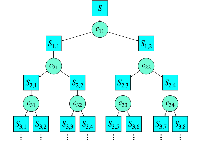
Figure 2: The partitioning of qubits according to the conditional independence assumption. $S_{i,j}$ represents the $j^{\mathrm{th}}$ subsystem at partition level $i$. $c_{ij}$ represents the conditional qubit that connects the subsystems $S_{i,2j-1}$ and $S_{i,2j}$. This partitioning scheme assumes that the subsystems are independent given the state of $c_{ij}$. This process allows us to factorize a joint probability distribution into conditional probability distributions.

The partitioning of the given quantum system based on the principle of conditional independence is illustrated in Fig. 2. In this figure, $S_{i,j}$ represents the $j^{\mathrm{th}}$ subsystem at partition level $i$, while $c_{ij}$ denotes the conditional qubit that connects the subsystems $S_{i,2j-1}$ and $S_{i,2j}$. This partitioning scheme assumes that the subsystems are independent given the state of $c_{ij}$. Let us denote a set of conditional qubits that connect a leaf $S_{i,j}$ and the root by $C_{S_{i,j}}$. For example, $C_{S_{3,3}}=\{c_{11},c_{21},c_{32}\}$ and $C_{S_{3,6}}=\{c_{11},c_{22},c_{33}\}$. The partitioning process continues until the leaf nodes are reached, where each leaf node consists of a small number of qubits (e.g., less than 10). For instance, if the partitioning in Fig. 2 terminates at level 3, we would have eight leaf nodes. Each leaf node is associated with a conditional probability distribution $p(S_{3,i}|C_{S_{3,i}})$, where $i\in\{1,\ldots,8\}$. The full joint probability distribution under CI is then computed by $\prod_{i=1}^{8}p(S_{3,i}|C_{S_{3,i}})\prod_{i=1}^{3}\prod_{j=1}^{2^{i-1}}p(c_{ij})$. In this example, each conditional probability distribution requires the training of eight separate neural networks, taking into account all computational basis states of the conditional qubits in $C_{S_{3,i}}$. However, the number of conditional qubits grows with the depth of the tree, which grows logarithmically with the number of total qubits. Moreover, it is evident that the number of leaf nodes cannot exceed the number of total qubits. Therefore, the number of neural networks to be trained independently grows linearly with the number of total qubits. The size of each neural network is constant because the leaf nodes are designed to contain only a small constant number of qubits. This constitutes an efficient QMEM method, which we refer to as CI-QMEM, that is exponentially faster than previous methods that aim to correct for the full joint probability distribution model without conditional independence, for which the size of the neural network or the size of the linear response matrix grows exponentially with the number of qubits.

The general formula for computing the joint probability distribution of a total system $S$ whose partitioning under CI terminates at level $L$ is

$$p(S)=\prod_{i=1}^{2^{L}}p(S_{L,i}|C_{S_{L,i}})\prod_{i=1}^{L}\prod_{j=1}^{2^{i-1}}p(c_{ij}).$$ (1)

III.2 Transfer Learning

Transfer learning (TL) can further reduce the training run-time by leveraging pre-trained neural networks. Instead of training a new neural network from scratch on a new dataset, transfer learning involves using parameters of a pre-trained network on a reference dataset that shares some similarities with the new dataset [36, 37, 38]. Typically, the lower (earlier) hidden layers of a neural network, which capture low-level features, are kept frozen, while only the upper (later) layers are fine-tuned or trained. This strategy eliminates the need to relearn the common low-level features, enabling faster convergence and reducing the overall training time.

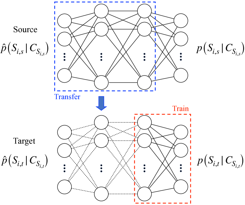
Figure 3: Transfer learning process for training neural networks in CI-QMEM. Initially, a neural network is trained to correct measurement errors of the source subsystem, denoted by $S_{i,s}$. The training utilizes the noisy probability distribution, $\hat{p}(S_{i,s}|C_{S_{i,s}})$ and $p(S_{i,s}|C_{S_{i,s}})$, as the input and the output, respectively. The parameters within the hidden layers, enclosed by a blue dashed box in the source model, are transferred to a new neural network designed to address measurement errors in a target subsystem, $S_{i,t}$. This transfer is achieved by initializing the dashed edges in the target neural network with their corresponding parameters from the source neural network. Subsequently, only the last hidden layer of the target model, represented by a red dashed box, undergoes training.

To understand how TL works in QMEM, let us consider a source subsystem denoted as $S_{i,s}$ with its associated conditional qubits represented by $C_{S_{i,s}}$. CI-QMEM trains a neural network for each computational basis state of the conditional qubits $C_{S_{i,s}}$ by utilizing the noisy and ideal conditional probability distributions, $\hat{p}(S_{i,s}|C_{S_{i,s}})$ and $p(S_{i,s}|C_{S_{i,s}})$, as input and output, respectively. Now, consider a target subsystem $S_{i,t}$ with the same number of qubits as $S_{i,s}$, also having its associated conditional qubits denoted by $C_{S_{i,t}}$. One might initially attempt repeat the entire CI-QMEM procedure described above to train a neural network for this new system. However, if the noise characteristics experienced by these subsystems exhibit similarities that can be captured by the neural network trained for the source system, it is unnecessary to train a separate neural network for the target system from the beginning. Instead, it is possible to transfer selected parameters learned from the source system to the target system, thereby reducing the number of parameters that need to be trained. Therefore, the application of TL is a justifiable approach, particularly when assuming the presence of systematic sources of noise that are common across different qubits within the quantum device. This concept is illustrated in Fig. 3. Importantly, a source model can be utilized for multiple target subsystems, as long as they share similar features with the source. Transfer learning typically reduces the number of parameters subject to training in the target model by a constant amount. Consequently, the reduction in trainable parameters also leads to a decrease in the amount of training data required for the model to converge. Henceforth, we refer to the QMEM technique that combines both CI and TL as CITL-QMEM.

IV Implementation

IV.1 Data collection

Deep learning-based QMEM methods require sample data for training neural networks. When constructing a family of quantum circuits to generate the training dataset, an essential requirement is the efficient computation of the associated probability distribution on a classical computer. This is necessary because training involves both noisy and ideal measurement results. Moreover, it is crucial that the error introduced by the gates used to prepare quantum states for the training data is negligible compared to the measurement error. In modern quantum devices, single-qubit gate errors are typically insignificant compared to measurement errors. Therefore, using quantum circuits composed solely of single-qubit gates satisfies these conditions.

Since the objective of QMEM is to mitigate errors in projective measurements in the computational basis, defined by the eigenstates of $\sigma_{z}$, the relative phase between computational basis states is irrelevant. Consequently, quantum circuits that generate training data employ only single-qubit $R_{y}(\theta)$ gates. Specifically, the unitary operation preparing the state is $\prod_{i=1}^{n}R^{(i)}{y}(\theta_{i})$, where the superscript $(i)$ denotes that the single-qubit rotation is applied to the $i^{\mathrm{th}}$ qubit. The rotation angles are sampled randomly in a way that resulting quantum states are distributed uniformly on the boundary of the $xz$-plane of the Bloch sphere. This is achieved by randomly generating values for $z_{i}\in[-1,1]$ and computing $\theta_{i}=\arccos(z_{i})$. The noisy probability distribution $\hat{\bm{p}}$ generated by the quantum circuit serves as the input for the neural network, while the ideal probability distribution $\bm{p}$ represents the desired output. The computation of $\bm{p}$ can be expressed as follows:

$$p(b)=\left|\prod_{i}^{n}\cos^{1-b_{i}}(\theta_{i}/2)\sin^{b_{i}}(\theta_{i}/2)\right|^{2},$$

where $b_{i}$ is the $i^{\mathrm{th}}$ bit of the binary string $b$.

In the LI-QMEM method, the training data comprises all computational basis states of the target qubit system, requiring $2^{n}$ circuit executions for an $n$-qubit system. The data acquisition and error mitigation process can be facilitated using the Qiskit Ignis package [39]. This package constructs a $2^{n}\times 2^{n}$ calibration matrix for the $n$-qubit system based on $2^{n}$ pairs of noisy and ideal results.

IV.2 Model construction

The neural network architecture comprises multiple layers, including the input, hidden, and output layers. For a joint probability distribution involving $n$ qubits, there exist $2^{n}$ possible computational basis states. Hence, both the input and output layers consist of $2^{n}$ nodes. To achieve an optimal balance between convergence speed and accuracy, thorough experimentation was conducted to select appropriate hyperparameters. Specifically, we configured the network with 4 hidden layers, and each hidden layer contained $5\times 2^{n}$ nodes. All hidden layers are fully connected layers, and each hidden node employs the Scaled Exponential Linear Unit (SELU) as the activation function [40, 23]. The output layer employs the softmax activation function, which normalizes the outputs into a probability distribution, ensuring that the sum of the output values is equal to one. The weights and biases of the neural network are optimised using the categorical cross-entropy loss function. The parameters are updated by the Adam optimizer [41]. As part of the hyperparameter tuning, we set the learning rate, batch size, and number of epochs to 0.0001, 16, and 300, respectively.

IV.3 Experimental Results

(a) ibmq_jakarta

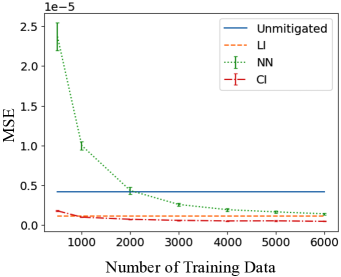
(b) ibm_lagos

Figure 4: Experimental results showing the mean squared error (MSE) between the ideal and error-mitigated probability distributions as a function of the number of training data. In the figure legend, we label the results from LI-QMEM, NN-QMEM, and CI-QMEM as LI, NN, and CI, respectively. The experiments were conducted on two 7-qubit devices: (a) ibmq_jakarta and (b) ibm_lagos. To evaluate the performance, 1500 test data points were used after training the model on varying numbers of training data. Each experiment was repeated five times, with the data set randomly split into training and test sets for each run. For NN and CI, the plotted values represent the mean MSE, with the error bars indicating one standard deviation. For the unmitigated and LI results, the smallest MSE obtained across the five experiments is shown.

To validate the effectiveness of the proposed QMEM methods and to compare their performances against existing ones, we conducted experiments on 7-qubit and 13-qubit quantum systems. We assessed the performance of different QMEM methods using three metrics: Mean Squared Error (MSE), Kullback-Leibler Divergence (KLD), and Infidelity (IF). These metrics quantify the dissimilarity between the ideal and mitigated probability distributions and are computed as follows:

$$D_{\mathrm{MSE}}={1\over 2^{n}}\sum_{i=1}^{2^{n}}\left|\tilde{p}_{i}-p_{i}\right|^{2},$$

$$D_{\mathrm{KLD}}=\sum_{i=1}^{2^{n}}p_{i}\log{{p_{i}}\over{\tilde{p}_{i}}},$$

$$D_{\mathrm{IF}}=1-\left(\sum_{i=1}^{2^{n}}\sqrt{p_{i}\tilde{p}_{i}}\right)^{2}.$$

Here, $p_{i}$ and $\tilde{p}_{i}$ represent the $i^{\mathrm{th}}$ elements of the vectors representing the ideal and the mitigated probability distributions, respectively. A lower value for these measures indicates better performance, as it signifies a closer match between the ideal and mitigated distributions. Additionally, to quantify the rate of error reduction, we use the rate of improvement for each loss function $D_{i}$, where the subscript $i$ corresponds to MSE, KLD, or IF. This rate of improvement, denoted as $R_{i}$, is calculated as follows [24]:

$$R_{i}=\frac{D_{i}^{\text{Unmitigated}}-D_{i}^{\text{QMEM}}}{D_{i}^{\text{Unmitigated}}}\times 100(\%).$$

A higher value of $R_{i}$ indicates better performance in reducing errors using QMEM.

The 7-qubit experiments were conducted using two IBM quantum devices, namely ibmq_jakarta and ibm_lagos. To obtain the calibration matrix for LI-QMEM, we generated a set of $2^{7}$ calibration circuits. For training the deep learning-based QMEM method, we generated 7500 data points for each device, which were then split into 6000 samples for training and 1500 samples for testing. To estimate the probability distribution, each quantum circuit was repeated $3.2\times 10^{4}$ times.

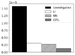
(a) MSE

(b) KLD

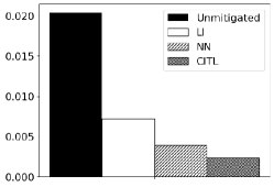
(c) Infidelity

Figure 5: To compare the 7-qubit QMEM results obtained using different methods on the ibmq_jakarta, we measured (a) MSE, (b) KLD, and (c) IF. The filled bars represent the unmitigated results, the unfilled bars represent the results obtained using the LI-QMEM method, the lighter hatched bars (third from the left) represent the results obtained using the NN-QMEM method, and the darker hatched bars (fourth from the left) represent the results obtained using the CITL-QMEM method.

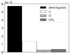
(a) MSE

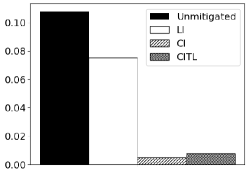
(b) KLD

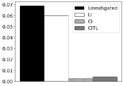
(c) Infidelity

Figure 6: To compare the 13-qubit QMEM results obtained using different methods on the ibmq_kolkata, we measured (a) MSE, (b) KLD, and (c) IF. The filled bars represent the unmitigated results, the unfilled bars represent the results obtained using the LI-QMEM method, the lighter hatched bars (third from the left) represent the results obtained using the CI-QMEM method, and the darker hatched bars (fourth from the left) represent the results obtained using the CITL-QMEM method.

		LI	NN	CI	CITL
	$R_{\mathrm{MSE}}$	80.47	82.56	91.76	91.91
ibmq_jakarta	$R_{\mathrm{KLD}}$	70.08	79.23	87.80	87.21
	$R_{\mathrm{IF}}$	64.68	80.64	88.24	87.54
	$R_{\mathrm{MSE}}$	72.02	63.27	87.96	89.32
ibm_lagos	$R_{\mathrm{KLD}}$	53.67	64.57	83.52	85.13
	$R_{\mathrm{IF}}$	43.29	66.67	84.20	85.76

Table 1: Performance evaluation of each QMEM method on the 7-qubit quantum devices, represented by the rate of improvement ($R_{i}$). The results for LI-QMEM, NN-QMEM, CI-QMEM, and CITL-QMEM are displayed in the first, second, third and fourth columns, respectively.

The results of the 7-qubit QMEM experiments for evaluating the MSE between the ideal and error-mitigated probability distributions as a function of the number of training data are shonw in Fig. 4. The results indicate that CI-QMEM achieves substantial error mitigation using less data compared to NN-QMEM. This observation is consistent with the well-known fact that the amount of data required for training deep neural networks depends on the model complexity [42, 43, 44, 45]. As CI-QMEM significantly reduces the size of neural networks and the number of model parameters, it improves the error mitigation performance, even with fewer data. Specifically, the conventional NN-QMEM trains a neural neural network with about $1.8\times 10^{6}$ parameters, while CI-QMEM uses only about $2.9\times 10^{4}$ parameters. The LI-QMEM, despite using only 128 data, cannot effectively mitigate non-linear errors as the deep learning-based approaches can. Consequently, CI-QMEM achieves smaller measurement errors, underscoring its superior performance in error mitigation compared to other methods. Based on the observation that the improvement from LI-QMEM to CI-QMEM is more pronounced in ibmq_jakarta compared to ibm_lagos, we speculate that the non-linear error is stronger in the former than in the latter. Moreover, it is important to note that the number of data required in LI-QMEM grows exponentially with the number of qubits.

CITL-QMEM, which incorporates TL in addition to CI, achieves a further reduction in the number of parameters to about $1.5\times 10^{4}$. This is accomplished by selecting the neural network trained for learning the conditional probability distribution, $p(q_{0},q_{1},q_{2}|q_{3})$, as the source model. Subsequently, the target model learns the new conditional probability distribution, $p(q_{4},q_{5},q_{6}|q_{3})$. In this TL approach, only the last layer of the target neural network is fine-tuned (trained), while the rest of the hidden layers retain the parameters from the source model.

The overall results for the 7-qubit QMEM are reported in Table  1, and Fig. 5 illustrates the effectiveness of transfer learning in reducing errors. Since the amount of error mitigated by CI-QMEM and CITL-QMEM is comparable as shown in the table, the figure only presents the results from the latter.

		LI	CI	CITL
	$R_{\mathrm{MSE}}$	51.35	93.65	94.40
ibmq_mumbai	$R_{\mathrm{KLD}}$	-20.82	92.09	92.25
	$R_{\mathrm{IF}}$	-31.75	94.21	94.34
	$R_{\mathrm{MSE}}$	76.01	95.38	93.68
ibm_kolkata	$R_{\mathrm{KLD}}$	30.11	95.53	92.78
	$R_{\mathrm{IF}}$	13.14	96.43	93.91

Table 2: Performance evaluation of each QMEM method on the 13-qubit quantum devices, represented by the rate of improvement ($R_{i}$). The results for LI-QMEM, CI-QMEM, and CITL-QMEM are displayed in the first, second, and third columns, respectively.

The 13-qubit QMEM experiments were conducted using two IBM quantum devices, namely ibmq_mumbai and ibmq_kolkata. These devices consist of 27 qubits, and for our experiment, we selected 13 of them as shown in Fig. 1b. We generated 6000 data for each device and split them into 5950 for training and 50 for testing. To estimate the probability distribution, we repeated the quantum circuit $1.0\times 10^{5}$ times, which is the maximum number available as the cloud service allows.

As shown in Fig. 1b. The joint probability distribution for the 13-qubit system decomposes as $\prod_{i=1}^{2^{2}}p(S_{2,i}|C_{S_{2,i}})\prod_{i=1}^{2}\prod_{j=1}^{2^{i-1}}p(c_{ij})$, where $S_{2,1}=\{q_{4},q_{6},q_{7}\}$, $S_{2,2}=\{q_{12},q_{15}\}$, $S_{2,3}=\{q_{5},q_{8},q_{9}\}$, $S_{2,4}=\{q_{14},q_{16}\}$, $c_{11}=q_{13}$, $c_{21}=q_{10}$, and $c_{22}=q_{11}$. Each conditional probability distribution requires training four separate neural networks, taking into account all computational basis states of the conditional qubits. Consequently, the total number of neural networks to be trained is $4\times 4+3=19$. For transfer learning, we selected $S_{2,1}$ and $S_{2,2}$ as source subsystems. The results are presented in Fig. 6 and Table 2. For the 13-qubit system, we did not perform conventional NN-QMEM experiments as it requires training a neural network with about $7.3$ billion parameters, leading to unreasonably long data collection and training times. As evident from both the figures and the table, our methods significantly reduce errors in all performance measures. Interestingly, on the ibmq_mumbai device, CITL-QMEM performs slightly better than CI-QMEM. This can be attributed to the use of a pre-trained model, enabling the creation of a simpler neural network with enhanced generalization capability [46, 47]. It is important to note that while LI-QMEM requires 8192 data points and NN-QMEM requires 7.3 billion parameters, our method is trained with only 5950 data points and $7.4\times 10^{4}$ parameters for CI-QMEM, and $3.9\times 10^{4}$ parameters for CITL-QMEM.

V Conclusions and Discussion

We introduced a scalable quantum measurement error mitigation method that overcomes the limitations of existing approaches. By utilizing conditional independence and transfer learning techniques, we achieve exponential reductions in the size of neural networks while maintaining excellent error-mitigation capabilities. Our method not only reduces the size of neural networks and the number of parameters to optimize but also significantly decreases the amount of data required for effective training. Experimental results on four IBM quantum devices, featuring 7 and 13 qubits, provide strong evidence of the efficiency and effectiveness of our method in mitigating measurement errors. Notably, CI-QMEM demonstrates a substantial reduction of neural network parameters by approximately 60 times for 7-qubit systems and $10^{5}$ times for 13-qubit systems. Transfer learning allows for the additional reduction of parameters by approximately a factor of two in both cases, leading to even more efficient training. As a result, CI-QMEM and CITL-QMEM consistently outperformed the full NN-QMEM under similar training conditions in all experiments. Moreover, these deep learing-based methods outperformed the LI-QMEM due to their ability to correct non-linear errors. In particular, for the 13-qubit experiments, the enhancements were achieved while using a smaller amount of data.

In the following, we discuss interesting future research directions and open problems. While the primary focus of this study is to mitigate measurement errors, the techniques developed here can be combined with existing methods for mitigating gate errors [13, 14, 48, 15, 16], thereby enhancing overall quantum computing performance. Integrating gate error mitigation approaches with measurement error mitigation techniques holds great potential for significant improvements in the accuracy and reliability of quantum computations. Moreover, it would be intriguing to extend the concepts of CI and TL explored in this work to improve the efficiency and scalability of the existing machine learning-based gate error mitigation technique [15]. The QMEM methods discussed in this work operate on the probability distribution obtained as the final outcome of a quantum computation at the software level. Consequently, these approaches are particularly suitable for cloud-based quantum computing environments. An interesting future endeavor is to optimize the performance by combining these approaches with hardware-level techniques that specifically addresses improving qubit-state-assignment fidelity by working directly with the readout signals [23]. Furthermore, the success of CI-QMEM implies that the underlying assumption of negligible measurement cross-talk among distant qubits holds. Exploring the reverse scenario and developing techniques to characterize measurement crosstalk by leveraging the concept of conditional independence presents an interesting avenue for future research. An important open problem in the general NN-QMEM, including our approach, pertains to the potential impact of shot noise in large systems. For instance, when working with training data that is close to a uniformly-distributed state, the number of shots required to obtain its noisy distribution grows exponentially with the number of qubits. Future research can explore the effectiveness of CI and TL based QMEM on a biased training set, where the smallest probability is in $O(1/\mathrm{poly(n)})$, or develop tailored methods for such conditions.

References

- [1] Peter W Shor. Polynomial-time algorithms for prime factorization and discrete logarithms on a quantum computer. SIAM review, 41(2):303–332, 1999.
- [2] Richard P Feynman. Simulating physics with computers. In Feynman and computation, pages 133–153. CRC Press, 2018.
- [3] Alberto Peruzzo, Jarrod McClean, Peter Shadbolt, Man-Hong Yung, Xiao-Qi Zhou, Peter J. Love, Alán Aspuru-Guzik, and Jeremy L. O’Brien. A variational eigenvalue solver on a photonic quantum processor. Nature Communications, 5(1):4213, July 2014.
- [4] Jarrod R McClean, Jonathan Romero, Ryan Babbush, and Alán Aspuru-Guzik. The theory of variational hybrid quantum-classical algorithms. New Journal of Physics, 18(2):023023, feb 2016.
- [5] Aram W Harrow, Avinatan Hassidim, and Seth Lloyd. Quantum algorithm for linear systems of equations. Physical review letters, 103(15):150502, 2009.
- [6] Patrick Rebentrost, Masoud Mohseni, and Seth Lloyd. Quantum support vector machine for big data classification. Phys. Rev. Lett., 113:130503, Sep 2014.
- [7] Seth Lloyd, Masoud Mohseni, and Patrick Rebentrost. Quantum principal component analysis. Nature Physics, 10(9):631–633, 2014.
- [8] Ashley Montanaro. Quantum speedup of monte carlo methods. Proceedings of the Royal Society A: Mathematical, Physical and Engineering Sciences, 471(2181):20150301, 2015.
- [9] Thomas J. Elliott, Chengran Yang, Felix C. Binder, Andrew J. P. Garner, Jayne Thompson, and Mile Gu. Extreme dimensionality reduction with quantum modeling. Phys. Rev. Lett., 125:260501, Dec 2020.
- [10] Carsten Blank, Daniel K. Park, and Francesco Petruccione. Quantum-enhanced analysis of discrete stochastic processes. npj Quantum Information, 7(1):126, August 2021.
- [11] Dorit Aharonov and Michael Ben-Or. Fault-tolerant quantum computation with constant error. In Proceedings of the twenty-ninth annual ACM symposium on Theory of computing, pages 176–188, 1997.
- [12] Austin G Fowler, Matteo Mariantoni, John M Martinis, and Andrew N Cleland. Surface codes: Towards practical large-scale quantum computation. Physical Review A, 86(3):032324, 2012.
- [13] Kristan Temme, Sergey Bravyi, and Jay M Gambetta. Error mitigation for short-depth quantum circuits. Physical review letters, 119(18):180509, 2017.
- [14] Suguru Endo, Simon C Benjamin, and Ying Li. Practical quantum error mitigation for near-future applications. Physical Review X, 8(3):031027, 2018.
- [15] Changjun Kim, Kyungdeock Daniel Park, and June-Koo Rhee. Quantum error mitigation with artificial neural network. IEEE Access, 8:188853–188860, 2020.
- [16] Tomochika Kurita, Hammam Qassim, Masatoshi Ishii, Hirotaka Oshima, Shintaro Sato, and Joseph Emerson. Synergetic quantum error mitigation by randomized compiling and zero-noise extrapolation for the variational quantum eigensolver. arXiv preprint arXiv:2212.11198, 2022.
- [17] John Preskill. Quantum computing in the nisq era and beyond. Quantum, 2:79, 2018.
- [18] Ying Li and Simon C Benjamin. Efficient variational quantum simulator incorporating active error minimization. Physical Review X, 7(2):021050, 2017.
- [19] Youngseok Kim, Andrew Eddins, Sajant Anand, Ken Xuan Wei, Ewout van den Berg, Sami Rosenblatt, Hasan Nayfeh, Yantao Wu, Michael Zaletel, Kristan Temme, and Abhinav Kandala. Evidence for the utility of quantum computing before fault tolerance. Nature, 618(7965):500–505, 2023.
- [20] Yanzhu Chen, Maziar Farahzad, Shinjae Yoo, and Tzu-Chieh Wei. Detector tomography on ibm quantum computers and mitigation of an imperfect measurement. Phys. Rev. A, 100:052315, Nov 2019.
- [21] Filip B. Maciejewski, Zoltán Zimborás, and Michał Oszmaniec. Mitigation of readout noise in near-term quantum devices by classical post-processing based on detector tomography. Quantum, 4:257, April 2020.
- [22] Hyeokjea Kwon and Joonwoo Bae. A hybrid quantum-classical approach to mitigating measurement errors in quantum algorithms. IEEE Transactions on Computers, 70(9):1401–1411, 2021.
- [23] Benjamin Lienhard, Antti Vepsäläinen, Luke C.G. Govia, Cole R. Hoffer, Jack Y. Qiu, Diego Ristè, Matthew Ware, David Kim, Roni Winik, Alexander Melville, Bethany Niedzielski, Jonilyn Yoder, Guilhem J. Ribeill, Thomas A. Ohki, Hari K. Krovi, Terry P. Orlando, Simon Gustavsson, and William D. Oliver. Deep-neural-network discrimination of multiplexed superconducting-qubit states. Phys. Rev. Applied, 17:014024, Jan 2022.
- [24] Jihye Kim, Byungdu Oh, Yonuk Chong, Euyheon Hwang, and Daniel K Park. Quantum readout error mitigation via deep learning. New Journal of Physics, 24(7):073009, 2022.
- [25] Sinno Jialin Pan and Qiang Yang. A survey on transfer learning. IEEE Transactions on knowledge and data engineering, 22(10):1345–1359, 2010.
- [26] Norbert M. Linke, Dmitri Maslov, Martin Roetteler, Shantanu Debnath, Caroline Figgatt, Kevin A. Landsman, Kenneth Wright, and Christopher Monroe. Experimental comparison of two quantum computing architectures. Proceedings of the National Academy of Sciences, 114(13):3305–3310, 2017.
- [27] C. Monroe, R. Raussendorf, A. Ruthven, K. R. Brown, P. Maunz, L.-M. Duan, and J. Kim. Large-scale modular quantum-computer architecture with atomic memory and photonic interconnects. Phys. Rev. A, 89:022317, Feb 2014.
- [28] Naomi H. Nickerson, Joseph F. Fitzsimons, and Simon C. Benjamin. Freely scalable quantum technologies using cells of 5-to-50 qubits with very lossy and noisy photonic links. Phys. Rev. X, 4:041041, Dec 2014.
- [29] Sergey Bravyi, Oliver Dial, Jay M. Gambetta, Darío Gil, and Zaira Nazario. The future of quantum computing with superconducting qubits. Journal of Applied Physics, 132(16):160902, 10 2022.
- [30] Edwin Tham, Ilia Khait, and Aharon Brodutch. Quantum circuit optimization for multiple qpus using local structure. In 2022 IEEE International Conference on Quantum Computing and Engineering (QCE), pages 476–483, 2022.
- [31] Ilia Khait, Edwin Tham, Dvira Segal, and Aharon Brodutch. Variational quantum eigensolvers in the era of distributed quantum computers. arXiv preprint arXiv:2302.14067, 2023.
- [32] Yordan S. Yordanov and Crispin H. W. Barnes. Implementation of a general single-qubit positive operator-valued measure on a circuit-based quantum computer. Phys. Rev. A, 100:062317, Dec 2019.
- [33] Dongkeun Lee, Kyunghyun Baek, Joonsuk Huh, and Daniel K Park. Variational quantum state discriminator for supervised machine learning. arXiv preprint arXiv:2303.03588, 2023.
- [34] A Philip Dawid. Conditional independence in statistical theory. Journal of the Royal Statistical Society Series B: Statistical Methodology, 41(1):1–15, 1979.
- [35] Daphne Koller and Nir Friedman. Probabilistic graphical models: principles and techniques. MIT press, 2009.
- [36] Matthew E Taylor and Peter Stone. Transfer learning for reinforcement learning domains: A survey. Journal of Machine Learning Research, 10(7), 2009.
- [37] Chuanqi Tan, Fuchun Sun, Tao Kong, Wenchang Zhang, Chao Yang, and Chunfang Liu. A survey on deep transfer learning. In Artificial Neural Networks and Machine Learning–ICANN 2018: 27th International Conference on Artificial Neural Networks, Rhodes, Greece, October 4-7, 2018, Proceedings, Part III 27, pages 270–279. Springer, 2018.
- [38] Colin Raffel, Noam Shazeer, Adam Roberts, Katherine Lee, Sharan Narang, Michael Matena, Yanqi Zhou, Wei Li, and Peter J Liu. Exploring the limits of transfer learning with a unified text-to-text transformer. The Journal of Machine Learning Research, 21(1):5485–5551, 2020.
- [39] Md Sajid Anis, Héctor Abraham, R Agarwal AduOffei, Gabriele Agliardi, Merav Aharoni, Ismail Yunus Akhalwaya, Gadi Aleksandrowicz, Thomas Alexander, Matthew Amy, Sashwat Anagolum, et al. Qiskit: An open-source framework for quantum computing. Qiskit/qiskit, 2021.
- [40] Günter Klambauer, Thomas Unterthiner, Andreas Mayr, and Sepp Hochreiter. Self-normalizing neural networks. In I. Guyon, U. Von Luxburg, S. Bengio, H. Wallach, R. Fergus, S. Vishwanathan, and R. Garnett, editors, Advances in Neural Information Processing Systems, volume 30. Curran Associates, Inc., 2017.
- [41] Diederik P Kingma and Jimmy Ba. Adam: A method for stochastic optimization. arXiv preprint arXiv:1412.6980, 2014.
- [42] Marvin Höge, Thomas Wöhling, and Wolfgang Nowak. A primer for model selection: The decisive role of model complexity. Water Resources Research, 54(3):1688–1715, 2018.
- [43] Laith Alzubaidi, Jinglan Zhang, Amjad J Humaidi, Ayad Al-Dujaili, Ye Duan, Omran Al-Shamma, José Santamaría, Mohammed A Fadhel, Muthana Al-Amidie, and Laith Farhan. Review of deep learning: Concepts, cnn architectures, challenges, applications, future directions. Journal of big Data, 8:1–74, 2021.
- [44] Xia Hu, Lingyang Chu, Jian Pei, Weiqing Liu, and Jiang Bian. Model complexity of deep learning: A survey. Knowledge and Information Systems, 63:2585–2619, 2021.
- [45] Iqbal H Sarker. Deep learning: a comprehensive overview on techniques, taxonomy, applications and research directions. SN Computer Science, 2(6):420, 2021.
- [46] Jason Yosinski, Jeff Clune, Yoshua Bengio, and Hod Lipson. How transferable are features in deep neural networks? Advances in neural information processing systems, 27, 2014.
- [47] Laith Alzubaidi, Mohammed A Fadhel, Omran Al-Shamma, Jinglan Zhang, Jorge Santamaría, Ye Duan, and Sameer R. Oleiwi. Towards a better understanding of transfer learning for medical imaging: a case study. Applied Sciences, 10(13):4523, 2020.
- [48] Kyle Willick, Daniel K. Park, and Jonathan Baugh. Efficient continuous-wave noise spectroscopy beyond weak coupling. Phys. Rev. A, 98:013414, Jul 2018.