Circumvent spherical Bessel function nulls for open sphere microphone arrays with physics informed neural network

Abstract

Open sphere microphone arrays (OSMAs) are simple to design and do not introduce scattering fields, and thus can be advantageous than other arrays for implementing spatial acoustic algorithms under spherical model decomposition. However, an OSMA suffers from spherical Bessel function nulls which make it hard to obtain some sound field coefficients at certain frequencies. This paper proposes to assist an OSMA for sound field analysis with physics informed neural network (PINN). A PINN models the measurement of an OSMA and predicts the sound field on another sphere whose radius is different from that of the OSMA. Thanks to the fact that spherical Bessel function nulls vary with radius, the sound field coefficients which are hard to obtain based on the OSMA measurement directly can be obtained based on the prediction. Simulations confirm the effectiveness of this approach and compare it with the rigid sphere approach.

Keywords: Microphone array signal processing, physics informed neural network, spherical harmonics.

1 Introduction

The products of the spherical harmonics (SHs) and the spherical Bessel functions (or the spherical Hankel functions) form the spherical nodes [williams2000fourier], a complete and orthogonal function set for the Helmholtz equation, the governing partial differential equation (PDE) of acoustic wave propagation. The SH decomposition of a sound field (the angular dependent SHs, the radial dependent spherical Bessel functions, and the frequency dependent sound field coefficients) greatly facilitates its analysis and manipulation [williams2000fourier, thushara_near_1999, Rafaely2015]. Thus, spherical modal decomposition has become popular in many diverse spatial acoustic applications, such as spatial active noise control [Wen_2018, ma2018active, Fei_2020], beamforming [5745011, Rafaely2015, huang2018insights], and direction of arrival estimation [moore2016direction, hafezi2017augmented, jo2019parametric].

Due to their simplicity, open sphere microphone arrays (OSMAs) are intuitively chosen for implementing the spherical modal decomposition [5745011]. However, the spherical Bessel function nulls make it hard to obtain some order of the sound field coefficients at certain frequencies with an OSMA. We can mitigate this problem through arranging microphones on a rigid sphere [5744968], inside a spherical shell, or using vector sensors on an open sphere [Rafaely2015, Ma2018, huang_flexible]. However, those approaches will unavoidably introduce scattering fields, request more microphones, and significantly increase the cost, respectively.

In this paper, we propose to circumvent the problem of spherical Bessel function nulls for an OSMA with the help of physics informed neural network (PINN) [raissi2019physics, cuomo2022scientific, karniadakis2021physics], a neural work which incorporates physical knowledge into its architecture and training. We model the measurement of an OSMA with a PINN, and then use it to predict the sound field on another sphere whose radius is different from that of the OSMA. Thanks to the fact that the spherical Bessel function nulls vary with radius, we can obtain the sound field coefficients which are difficult to obtain with the OSMA measurement based on the predicted sound field. The effectiveness of this approach is confirmed by simulations and compared with the rigid sphere approach.

2 Problem formulation

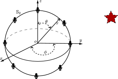
Figure 1: A microphone array on an open sphere and some sound sources $\star$.

We consider the set up shown in Fig. 1, where there are $Q$ omni-directional pressure microphones on an open sphere $\mathbb{S}_{2}$ of radius $r_{a}$ and some sound sources. The Cartesian coordinates and the spherical coordinates of a point with respect to an origin are denoted as $O$ as $(x,y,z)$ and $(r,\theta,\phi)$, respectively [Rafaely2015]. One would like to reconstruct the sound field around the sphere or locate the sound sources based on the OSMA measurement.

The tasks could be approached with SH decomposition. We decompose the sound pressure at microphone position $\{(r_{a},\theta_{q},\phi_{q})\}_{q=1}^{Q}$ onto SHs as [williams2000fourier] rcl P(ω,r_a,θ_q,ϕ_q) &≈∑_u=0^U∑_v=-u^uP_u,v(ω,r_a)Y_u,v(θ_q,ϕ_q)
=∑_u=0^U∑_v=-u^uK_u,v(ω) j_u(ωr_a/s)
×Y_u,v(θ_q,ϕ_q), where $\omega=2\pi{f}$ is the angular frequency ($f$ is the frequency), $s$ is the speed of sound propagation, $U=\lceil{2\pi{f}r_{a}/s}\rceil$ is the up-order of the SHs that are needed to represent the sound pressure accurately [Thusharahigh] ($\lceil{\cdot}\rceil$ is the ceiling operation),. $\mathsf{P}_{u,v}(\omega,r_{a})$ are the pressure field coefficients, $\mathsf{K}_{u,v}(\omega)$ are the sound field coefficients [williams2000fourier], $j_{u}(\cdot)$ is the spherical Bessel function of the first kind of order $u$, $Y_{u,v}(\theta,\phi)$ is the SH of order $u$ and degree $v$ [williams2000fourier] at is evaluated at $(\theta,\phi)$.

The sound field coefficients $\mathsf{K}_{u,v}(\omega)$ characterize the sound sources and allow us to reconstruct the sound field or to locate the sound sources [Rafaely2015]. To obtain the sound field coefficients, we first estimate the pressure field coefficients through [Rafaely2015] rcl ^P_u,v(ω,r_a)=∑_q=1^Q P(ω,r_a,θ_q,ϕ_q)Y_u,v(θ_q,ϕ_q)γ_q, where $\{\gamma_{q}\}_{q=1}^{Q}$ are the sampling weights, and then estimate the sound field coefficients through rcl ^K_u,v(ω) &=^P_u,v(ω,r_a)/j_u(ωr_a/s). The problem with (1) is the spherical Bessel function ${j}_{u}(\cdot)$ nulls [Rafaely2015, Ma2018, huang_flexible]. Figure 2 presents $j_{u}(2\pi{f}r_{a}/s)$ with $r_{a}=0.05$ m, $s=343$ m/s, $u=0,1,2,3,4$. We can see that $j_{0}(2\pi{f}r_{a}/s)=0$ for $f=3430$ Hz, and $j_{1}(2\pi{f}r_{a}/s)=0$ for $f=4905$ Hz. This makes it difficult to estimate the sound field coefficients of order 0, $\mathsf{K}_{0,0}(\omega)$, and order 1, $\mathsf{K}_{1,v}(\omega)$, at frequency 3430 Hz and 4905 Hz with an OSMA array of radius $r_{a}=0.05$ m.

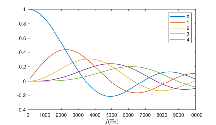
Figure 2: The spherical Bessel function $j_{u}(2\pi{f}r_{a}/s)$ as a function of frequency, $r_{a}=0.05$ m, $s=343$ m/s, $u=0,1,2,3,4$.

In this paper, we aim to circumvent the problem of spherical Bessel function nulls for an OSMA.

3 PINN Assisted OSMA

In this section, we propose a PINN method to assist an OSMA for sound field analysis. To simplify the calculation of the Laplacian, we express acoustic quantities in Cartesian coordinates.

The key idea is to exploit the fact that spherical Bessel function nulls vary with radius. The spherical Bessel function $j_{u}(\cdot)$ is a function of both frequency $f$ and radius $r$, and thus that $j_{u}(2\pi{f}r_{b}/s)\neq 0$ if $r_{b}{}\neq{}r_{a}$ and $j_{u}(2\pi{f}r_{a}/s)=0$. Thus that we can obtain the sound field coefficients which are difficult to obtain with an OSMA of radius $r_{a}$ based on the sound field on another sphere of radius $r_{b}$. An OSMA of radius $r_{a}$ can not measure the sound field on another sphere of radius $r_{b}$ directly, but we can build a PINN [raissi2019physics, cuomo2022scientific, karniadakis2021physics] to predict the sound field on the other sphere based on the measurement of the OSMA.

We build up a $L$ layer $N$ node (on each layer) full connected feedforward neural network [raissi2019physics] whose inputs are Cartesian coordinates $(x,y,z)$ and output is the sound field estimation $\hat{P}_{\mathrm{PI}}(\omega,x,y,z)$, and update the trainable parameters of the network by minimizing the following cost function rcl &L= ⏟1Q∑_q=1^Q∥ P(ω,x_q,y_q,z_q)- ^P_PI(ω,x_q,y_q,z_q) ∥_2^2 _L_data
+⏟1A∑_a=1^A ∥ ∇^PPI(ω,xa,ya,za) (w/s)2+^P_PI(ω,x_a,y_a,z_a) ∥_2^2 _L_PDE,    where $\|\cdot\|_{2}$ is the 2-norm, $\nabla\equiv\frac{\partial^{2}}{\partial{}x^{2}}+\frac{\partial^{2}}{\partial{}y^{2}}+\frac{\partial^{2}}{\partial{}z^{2}}$ is the Laplacian. The data loss $\mathfrak{L}_{\mathrm{data}}$ makes the network output to approximate the OSMA measurement $\{P(\omega,x_{q},y_{q},z_{q})\}_{q=1}^{Q}$ where $(x_{q},y_{q},z_{q})_{q=1}^{Q}$ correspond to $(r_{a},\theta_{q},\phi_{q})_{q=1}^{Q}$. The PDE loss $\mathfrak{L}_{\mathrm{PDE}}$ informs the network output to conform with the Helmholtz equation on the measurement sphere of radius $r_{a}$, where $\{(x_{a},y_{a},z_{a})\}_{a=1}^{A}$ are uniformly arranged sampling points on the sphere.

To obtain the sound field coefficients, we first train the PINN and use it to estimate the pressure $\hat{P}_{\mathrm{PI}}(\omega,x_{d},y_{d},z_{d})$ (which are equal to $\hat{P}_{\mathrm{PI}}(\omega,r_{b},\theta_{d},\phi_{d})$) on a sphere of radius $r_{b}$. Next we estimate the pressure field coefficients $\hat{\mathsf{P}}_{u,v}(\omega,r_{b})$ rcl ^P_u,v(ω,r_b)=∑_d=1^D ^P_PI(ω,r_b,θ_d,ϕ_d)Y_u,v(θ_d,ϕ_d)γ_d, where $\{\gamma_{d}\}_{d=1}^{D}$ are the sampling weights [Rafaely2015]. We further estimate the sound field coefficients through rcl ^K_u,v(ω) &= ^P_u,v(ω,r_b)/j_u(ωr_b/s). In summary, for spatial acoustics with an OSMA, we can estimate the sound field coefficients through (1) when $j_{u}(kr_{a})\neq 0$ and through (3), (3), (3) when $j_{u}(kr_{a})=0$. In this way, the problem of spherical Bessel function nulls is circumvented.

Note that the spherical Bessel function nulls is a problem under the spherical modal decomposition, but it is not a problem with the PINN. This is the fundamental fact that make the PINN assisted OSMA sound field analysis possible.

4 Simulation

In this section, we use a sound field reconstruction task to demonstrate the performance of the PINN assisted OSMA and compare it with the rigid sphere approach.

We consider the setup shown in Fig. 1. There is a radius $r_{a}=0.05$ m OSMA with 36 uniformly arranged omni-directional pressure microphones on it. There is a sound source located at $(0.5\;\mathrm{m,0.5\;\mathrm{m}},0.75\;\mathrm{m})$. The sound source generates a unit amplitude sinusoidal signal at $f=3430$ Hz. In the case, the up-order of SHs needed to represent the sound field is $U=\lceil{2\pi\times 3430\times 0.05/343}\rceil$ = 4 [Thusharahigh]. The transfer functions between the sound source and the microphones are simulated based on the Green’s function [williams2000fourier]. The aim is to reconstruct the sound field on a smaller sphere of radius $r_{c}=0.04$ m.

Three approaches for sound field reconstruction are considered. The first is the OSMA approach based on the spherical modal decomposition. For this approach, we estimate the sound field coefficients $\{\hat{\mathsf{K}}_{u,v}(\omega)\}_{u=1}^{4}$ through (1) and reconstruct the sound field on the smaller sphere by rcl ^P_SH(ω,r_c,θ,ϕ) &≈∑_u=1^U∑_v=-u^u^K_u,v(ω) j_u(ωr_c/s) Y_u,v(θ,ϕ),   because $\hat{\mathsf{K}}_{0,0}(\omega)$ is not obtainable.

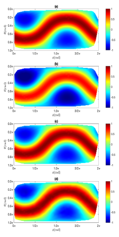
Figure 3: Sound field at $f=3430$ Hz : (a) the ground truth, (b) OSMA reconstruction, (c) PINN assisted OSMA reconstruction, and (d) the rigid sphere reconstruction.

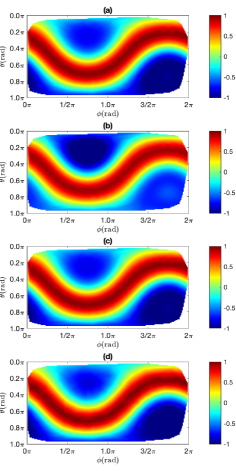
Figure 4: Sound field at $f=4905$ Hz : (a) the ground truth, (b) OSMA reconstruction, (c) PINN assisted OSMA reconstruction, and (d) the rigid sphere reconstruction.

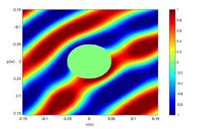
Figure 5: The scattering field around a rigid sphere at 3430 Hz.

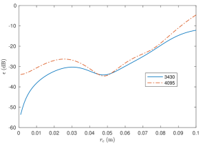
Figure 6: Sound field reconstruction error $\epsilon$ of the pure PINN method as a function of the reconstruction sphere radius $r$ at 3430 Hz and 4095 Hz.

The second one is the PINN assisted OSMA method. For this method, we build up a $L=3$ layer and $N=3$ node PINN, with the activation function being $\tanh$, and initialize the trainable parameters with the Xavier initialization [glorot2010understanding]. PINN is trained for 10⁸ epochs with a learning rate of 10^-5 using the ADAM optimizer. The data loss $\mathfrak{L}_{\mathrm{data}}$ is evaluated with respect to the 36 microphone measurements, and the PDE losses $\mathfrak{L}_{\mathrm{PDE}}$ with respect to the Cartesian coordinates of 500 uniformly arranged sampling points on the sphere of radius $r_{a}=0.05$ m. We first estimate the sound field coefficients $\{\hat{\mathsf{K}}_{u,v}(\omega)\}_{u=1}^{4}$ through (1), $\hat{\mathsf{K}}_{0,0}(\omega)$ through (3), (3) with (3) with $r_{b}=0.048$ m, and next reconstruct the sound field on the smaller sphere similar as (4) but with $\hat{K}_{0,0}(\omega)j_{u}(\omega{r_{c}}/s)Y_{0,0}(\theta,\phi)$ included.

The third one is the rigid sphere approach. The OSMA in Fig. 1 is replaced with a rigid sphere of the same radius, and the rest of simulation setting is the same. we reconstruct the sound field on the sphere of radius $r_{c}$ as rcl P(ω,r_c,θ,ϕ)&≈∑_u=0^U G_u(ω,r_c,r