An increasing rank Riemannian method for generalized Lyapunov equations

Abstract

In this paper, we consider finding a low-rank approximation to the solution of a large-scale generalized Lyapunov matrix equation in the form of $AXM+MXA=C$, where $A$ and $M$ are symmetric positive definite matrices. An algorithm called an Increasing Rank Riemannian Method for Generalized Lyapunov Equation (IRRLyap) is proposed by merging the increasing rank technique and Riemannian optimization techniques on the quotient manifold $\mathbb{R}_{*}^{n\times p}/\mathcal{O}_{p}$. To efficiently solve the optimization problem on $\mathbb{R}_{*}^{n\times p}/\mathcal{O}_{p}$, a line-search-based Riemannian inexact Newton’s method is developed with its global convergence and local superlinear convergence rate guaranteed. Moreover, we derive a preconditioner which takes $M\neq I$ into consideration. Numerical experiments show that the proposed Riemannian inexact Newton’s method and preconditioner has superior performance and IRRLyap is preferable compared to the tested state-of-the-art methods when the lowest rank solution is desired.

Keywords: Generalized Lyapunov equations, Riemannian optimization, Low-rank approximation, Riemannian truncated Newton’s method, Increasing rank method

1 Introduction

This paper considers the large-scale generalized Lyapunov matrix equation

$$AXM+MXA-C=0,$$ (1.1)

where $A,M\in\mathbb{R}^{n\times n}$ are large-scale, sparse, and symmetric positive definite matrices and $C\in\mathbb{R}^{n\times n}$ is symmetric positive semidefinite. It has been shown in [Chu87, Pen98] that Equation (1.1) has a unique solution $X^{*}$ and $X^{*}$ is symmetric positive semidefinite. Moreover, it is known that under certain circumstances such as $C$ is low rank, the solution $X^{*}$ of the Lyapunov equation (1.1) can be well approximated by a low-rank matrix, since the eigenvalues of the solution $X^{*}$ numerically has an exponential decay [Pen00, Gra04].

In recent years, solving Equation (1.1) has attracted much attention since it plays a significant role in model reduction [Moo81, SVdVR08, HJR21, GGB22], signal processing [GDA⁺20], systems and control theory [J9́6, Ant05], and solutions of PDEs [PS16]. Equation (1.1) with a large-scale sparse system matrix $A$ and a large-scale sparse mass matrix $M$ can be yielded by the finite element method semidiscretized in space [VV10].

1.1 Contributions

In this paper, Problem (1.1) is formulated as an optimization problem on a quotient manifold $\mathbb{R}_{*}^{n\times p}/\mathcal{O}_{p}$ (see definition in Section 2). A line-search-based Riemannian truncated Newton’s method is developed by using the truncated Newton in [DS83a] and the line search conditions in [BN89]. The global convergence and local superlinear convergence rates are established. As far as we know, this is the first line-search-based generic Riemannian inexact Newton’s method for optimization and guarantees global and local superlinear convergence. In addition, the line search conditions that we used allow conditions other than the Wolfe conditions in [DS83a]. We equip the quotient manifold $\mathbb{R}_{*}^{n\times p}/\mathcal{O}_{p}$ with a Riemannian metric in [ZHVZ23] and explore the performance of the Riemannian truncated Newton’s method for solving (1.1). Moreover, we propose an new preconditioner which is more effective compared to the one in [VV10] in the sense that the new one takes $M\neq I$ into consideration whereas the one in [VV10] does not. We finally combine the Riemannian truncated Newton’s method with the increasing rank algorithm in [VV10] and give Algorithm 4 for solving (1.1). Numerically, the proposed Riemannian truncated Newton’s method is able to find higher accurate solutions compared to the Riemannian trust-region Newton’s method in [ABG07], the Riemannian conjugate gradient method [BA15], and the Riemannian memory-Limited BFGS method [HAGH18]; the proposed preconditioner can further reduce the number of actions of the Hessian evaluations when $M\neq I$ compared to the pre-conditioner in [VV10]; and the increasing rank method with the Riemannian truncated Newton’s method is able to find lower rank solutions compared to the three state-of-the-art low-rank methods K-PIK [Sim07], RKSM [DS11, KS20], and mess_lradi [SKB22] when the residual $\|AXM+MXA-C\|_{F}$ is roughly the same.

1.2 Related Work

Classical numerical methods for the standard Lyapunov matrix equations, i.e., setting $M=I$, include the Bartels-Stewart method [BS72], the Hessenberg–Schur method [GNVL79], and the Hammarling method [Ham82]. These methods are direct methods and the computations involve $O(n^{3})$ number of floating point operations, which prevents the use for large-scale problems, where the floating point operation is defined in [GL96]. One approach to develop an efficient method for large-scale problems is to explore the low-rank structure of the solution $X^{*}$.

Low-rank methods for Lyapunov equations.

In practice, there is a class of applications of generalized Lyapunov equation (1.1), whose solution can be approximated with a low-rank matrix of rank $p\ll n$. In this case, the number of unknowns is reduced to $np$, which is greatly less than $n^{2}$. If we can compute a low-rank approximation in $O(np^{c})$ operations with constant $c$, for large problems, then the complexity is significantly reduced. Based on this idea, very diverse low-rank methods have been proposed. Majority of these methods are based on Smith method [GSA03], low-rank alternating direction implicit iterative (LR-ADI) [LW04, BLT09, BK14, BPS22], sign function methods [BB06, Bau08], Krylov subspace techniques [Sim07, DS11, HJR21], and Riemannain optimization [VV10]. It is worth noting that there exist several low-rank methods for algebraic Riccati equations [MV14, BHW21], which, in some cases, are also suited for Lyapunov equations.

The low-rank methods listed above in addition to [VV10, MV14] all start from well-known iterative methods and skillfully rewrite the problem so that the problem can be transformed into a low-rank setting. Although the calculations of these methods are cheap at each step since they work on a factor $Y$ of iterate $X=YY^{T}$, the convergence rate of these methods is usually unknown or at most linear and no good acceleration strategy has been given. As a consequence, Bart et al. [VV10] reformulated Equation (1.1) into an optimization problem defined on the set of fixed rank symmetric positive semidefinite matrices. In this paper, we follow this idea but from the perspective of quotient manifold and propose a Riemannian Newton’s method to solve the problem. Moreover, it is empirically shown in Section 7.2 that the quotient manifold geometry is superior to the embedded submanifold geometry and the intuition is also discussed therein.

Riemannian Newton’s methods.

Newton’s method is a powerful tool for finding the minimizer of nonlinear functions in Euclidean spaces. Although Newton’s method has a fast local convergence rate, it is highly sensitive to the initial iterate (i.e., it is not globally convergent); it is not defined at points where the Hessian is singular; and for non-convex problems, it does not necessarily generate a sequence of descent directions. In order to overcome these issues, Dembo et al. [DS83a] proposed a truncated-Newton’s method. The truncated-Newton’s method contains two parts. The outer iteration executes Newton’s method based on line search, and the inner iteration solves the Newton equation inexactly by a truncated conjugate gradient method. Absil et al. [ABG07] proposed a Riemannian trust-region Newton’s method similar to this idea which is based on the trust-region method. The proposed method is a generalization of the one in [DS83a] to manifolds and further relaxes the line search condition used in [DS83a]. It is worth mentioning that there are some Riemannian Newton’s methods based on line search; see, e.g., [dABFFY18, ZBJ18, WZB20, dABFF22]. As far as we know, all the existing Riemannian Newton’s methods aim to find a root of a vector field, whereas the proposed Riemannian truncated-Newton’s method is used to optimize a sufficiently smooth function.

1.3 Outline

This paper is stated as follows. In Section 2, we introduce preliminaries on algebra and manifold. In Section 3, we reformulate Equation (1.1) as an optimization problem on quotient manifold $\mathbb{R}_{*}^{n\times p}/\mathcal{O}_{p}$. The classical truncated Newton’s method is generalized to Riemannian setting in Section 4 and it is proven that the proposed Riemannian truncated Newton’s method converges to a stationary point from any starting point and has a local superlinear convergence rate. In Section 5, we give ingredients for optimization on Riemannian quotient manifolds with three metrics. In Section 6, the proposed preconditioner is discussed, and the increasing rank algorithm for solving Equation (1.1) is given. Subsequently, in Section 7, we demonstrate the performance of the proposed Riemannian truncated-Newton’s method preconditioner, and compare the proposed method with other existing low-rank methods for Lyapunov equations. Finally, concluding remarks are given in Section 8.

2 Preliminaries and Notation

Throughout this paper, we denote the real matrices space of size $m$-by-$n$ by $\mathbb{R}^{m\times n}$. For $A\in\mathbb{R}^{m\times n}$, the matrix $A^{T}\in\mathbb{R}^{n\times m}$ denotes the transpose of $A$. Define $\mathrm{vec}(\cdot):\mathbb{R}^{m\times n}\rightarrow\mathbb{R}^{mn}$ as an isomorphism operator which transforms a matrix into a vector by column-wise stacking, that is, for any $A=[a_{1},a_{2},\cdots,a_{n}]\in\mathbb{R}^{m\times n}$. We have $\mathrm{vec}(A)=[a_{1}^{T},a_{2}^{T},\dots,a_{n}^{T}]\in\mathbb{R}^{mn}$. Let $\otimes$ denote the Kronecker product, i.e., for $A=[a_{ij}]\in\mathbb{R}^{m\times n}$ and $B=[b_{ij}]\in\mathbb{R}^{p\times q}$, it holds that $A\otimes B=[a_{ij}B]\in\mathbb{R}^{mp\times nq}$.

Riemannian geometry.

The Riemannian geometry and optimization used in this paper can be found in the standard literatures, e.g., [Boo75, AMS08], and the notation below follows [AMS08]. Denote a manifold by $\mathcal{M}$. For any $x\in\mathcal{M}$, $\mathrm{T}_{x}\mathcal{M}$ is the tangent space of $\mathcal{M}$ at $x$ and elements in $\mathrm{T}_{x}\mathcal{M}$ are call tangent vectors of $\mathcal{M}$. Tangent bundle, $\mathrm{T}\mathcal{M}$, of manifold $\mathcal{M}$ is the union set of all tangent spaces. Mapping $\eta:\mathcal{M}\rightarrow\mathrm{T}\mathcal{M}$ maps a point $x\in\mathcal{M}$ into a tangent vector $\eta_{x}\in\mathrm{T}_{x}\mathcal{M}$ and is called a vector field. A metric on a manifold $\mathcal{M}$ is defined as $g(\cdot,\cdot):\mathrm{T}\mathcal{M}\oplus\mathrm{T}\mathcal{M}\rightarrow\mathbb{R}$, where $\mathrm{T}\mathcal{M}\oplus\mathrm{T}\mathcal{M}=\{(\eta_{x},\xi_{x}):x\in\mathcal{M},\eta_{x}\in\mathcal{T}_{x}\mathcal{M},\xi_{x}\in\mathrm{T}_{x}\mathcal{M}\}$ is the Whitney sum of tangent bundle. Given $\eta_{x}\in\operatorname{\mathrm{T}}_{x}\mathcal{M}$, its induced norm is defined by $\|\eta_{x}\|=\sqrt{g(\eta_{x},\eta_{x})}$. If $g$ is smooth in the sense that for any two smooth vector fields $\xi$ and $\eta$, function $g(\xi,\eta):\mathcal{M}\rightarrow\mathbb{R}$ is smooth, then $\mathcal{M}$ equipped with $g$ is a Riemannian manifold and $g$ is called a Riemannian metric. If $\mathcal{M}$ is a Riemannian manifold, then the tangent space $\mathrm{T}_{x}\mathcal{M}$ is a Euclidean space with the Euclidean metric $g_{x}(\cdot,\cdot)=g(\cdot,\cdot)|_{\mathrm{T}_{x}\mathcal{M}}$. For a smooth function $f:\mathcal{M}\rightarrow\mathbb{R}$, notations $\mathrm{grad}f(x)$ and $\mathrm{Hess}f(x)$ denote the Riemannian gradient and Hessian of $f$ at $x$ respectively, and the action of $\mathrm{Hess}f(x)$ on a tangent vector $\eta_{x}\in\mathrm{T}_{x}\mathcal{M}$ is denoted by $\mathrm{Hess}f(x)[\eta_{x}]$. Let $\mathcal{H}_{x}$ be a linear operator on $\operatorname{\mathrm{T}}_{x}\mathcal{M}$. Its adjoint operator, denoted by $\mathcal{H}_{x}^{*}$, satisfies $g_{x}(\eta_{x},\mathcal{H}_{x}\xi_{x})=g_{x}(\mathcal{H}^{*}_{x}\eta_{x},\xi_{x})$ for all $\eta_{x},\xi_{x}\in\operatorname{\mathrm{T}}_{x}\mathcal{M}$. With $\mathcal{H}_{x}=\mathcal{H}_{x}^{*}$, we call $\mathcal{H}_{x}$ self-adjoint with respect to $g$.

Let $\gamma:\mathcal{I}\rightarrow\mathcal{M}$ denote a smooth curve and $\dot{\gamma}(t)\in\mathrm{T}_{\gamma(t)}\mathcal{M}$ denotes its velocity at $t$, where $\mathcal{I}\subset\mathbb{R}$ is open and $[0,1]\subset\mathcal{I}$. The distance between $x=\gamma(0)$ and $y=\gamma(1)$ is defined by $\mathrm{dist}(x,y)=\inf_{\{\gamma:\gamma(0)=x,\gamma(1)=y\}}\int_{0}^{1}\|\dot{\gamma}(t)\|\mathrm{d}t$. A smooth curve $\gamma:[0,1]\rightarrow\mathcal{M}$ is called the geodesic if it locally minimizes the distance between $\gamma(0)=x$ and $\gamma(1)=y$. Notation $B_{\mu}(0_{x})=\{\xi_{x}\in\mathrm{T}_{x}\mathcal{M}:\|\eta_{x}\|\leq\mu\}$ is used to denote the open ball in $\mathrm{T}_{x}\mathcal{M}$ of radius $\mu$ centered at $0_{x}$ and $B_{\mu}(x)=\{y\in\mathcal{M}:\mathrm{dist}(x,y)\leq\mu\}$ is an open ball in $\mathcal{M}$ of radius $\mu$ centered at $x$. A retraction $R:\operatorname{\mathrm{T}}\mathcal{M}\rightarrow\mathcal{M}$ is a map satisfying (i) $R(0_{x})=x$ for all $x\in\mathcal{M}$ and (ii) for each fixed $x\in\mathcal{M}$, $\frac{\mathrm{d}}{\mathrm{d}t}R(t\eta_{x})\big{|}_{t=0}=\eta_{x}$ for all $\eta_{x}\in\operatorname{\mathrm{T}}_{x}\mathcal{M}$.

The considered manifold.

The set of symmetric positive semidefinite matrices of size $n$ with fixed rank $p$, denoted by $\mathcal{S}_{+}(p,n)$, is a Riemannian manifold with dimension $np-\frac{1}{2}p(p-1)$ (see, e.g., [HS95]). For any $X\in\mathcal{S}_{+}(p,n)$, there exists a matrix $Y\in\mathbb{R}^{n\times p}_{*}$ such that $X=YY^{T}$, where $\mathbb{R}^{n\times p}_{*}=\{Y\in\mathbb{R}^{n\times p}:\mathrm{rank}(Y)=p\}$ is called a noncompact Stiefel manifold [AMS08, Chapter 3]. The orthogonal group $\mathcal{O}_{p}=\{O\in\mathbb{R}^{p\times p}:O^{T}O=I_{p}\}$ is a Lie group with the group operator given by the matrix product; it can be equipped with the smooth structure as an embedded submanifold of $\mathbb{R}^{p\times p}$; and its identity is the identity matrix $I_{p}$. Define a right group action of $\mathcal{O}_{p}$ on $\mathbb{R}^{n\times p}_{*}$ as:

$$\theta:\mathbb{R}^{n\times p}_{*}\times\mathcal{O}_{p}\rightarrow\mathbb{R}^{n\times p}_{*}:\theta(Y,Q)=YQ.$$

Obviously, this group action satisfies the identity and compatibility conditions [Bou20, Definition 9.11], and therefore it induces an equivalent relation $\sim$ on $\mathbb{R}^{n\times p}_{*}$:

$$Z\sim Y\Leftrightarrow Y=\theta(Z,Q)=ZQ\text{ for some }Q\in\mathcal{O}_{p}.$$

The orbit of $Y$ forms an equivalence class, namely, $[Y]=\{YQ:Q\in\mathcal{O}_{p}\}$. We denote the quotient space $\mathbb{R}^{n\times p}_{*}/\sim$ as $\mathbb{R}_{*}^{n\times p}/\mathcal{O}_{p}$. The natural projection between $\mathbb{R}^{n\times p}_{*}$ and $\mathbb{R}_{*}^{n\times p}/\mathcal{O}_{p}$ is given by

$$\pi:\mathbb{R}^{n\times p}_{*}\rightarrow\mathbb{R}^{n\times p}_{*}/\mathcal{O}_{p}:Y\mapsto\pi(Y)=[Y].$$

From now on, out of clarity, we denote $[Y]$ by $\pi(Y)$ as an element of the quotient manifold $\mathbb{R}_{*}^{n\times p}/\mathcal{O}_{p}$ and use $\pi^{-1}(\pi(Y))$ to denote $[Y]$ when it is regarded as a subset of $\mathbb{R}_{*}^{n\times p}$.

Since the Lie group $\mathcal{O}_{p}$ acts smoothly, freely and properly with the group action $\theta$ on the smooth manifold $\mathbb{R}^{n\times p}_{*}$, by [Bou20, Theorem 9.17], the quotient space $\mathbb{R}^{n\times p}_{*}/\mathcal{O}_{p}$ is a manifold called a quotient manifold of $\mathbb{R}^{n\times p}_{*}$. The manifold $\mathbb{R}_{*}^{n\times p}$ is therefore called the total space of $\mathbb{R}^{n\times p}_{*}/\mathcal{O}_{p}$. Since $\mathbb{R}^{n\times p}_{*}/\mathcal{O}_{p}$ is diffeomorphic to $\mathcal{S}_{+}(p,n)$, the quotient manifold $\mathbb{R}^{n\times p}_{*}/\mathcal{O}_{p}$ can be viewed as a representation of the manifold $\mathcal{S}_{+}(p,n)$.

Function classes.

For the convergence analysis, we need notions of a pullback of a real-valued function $f$ with respect to a retraction $R$ and the radially Lipschitz continuous differentiability of a pullback.

Definition 2.1.

Let $f:\mathcal{M}\rightarrow\mathbb{R}^{n}$ be a real-valued function on manifold $\mathcal{M}$ with a retraction $R$. We call $\hat{f}:\mathrm{T}\mathcal{M}\rightarrow\mathbb{R}:\eta_{x}\mapsto\hat{f}(\eta_{x})=f(R(\eta_{x}))$ the pullback of $f$ with respect to $R$. When restricted on $\mathrm{T}_{x}\mathcal{M}$, we denote $\hat{f}\big{|}_{\mathrm{T}_{x}\mathcal{M}}$ by $\hat{f}_{x}$.

Definition 2.2.

([AMS08, Definition 7.4.1]) Let $\hat{f}$ be a pullback of $f$ with respect to a retraction $R$. $\hat{f}$ is referred to as a radially $L$-$C^{1}$ function for all $x\in\mathcal{M}$ if there exists a positive constant $L$ such that for all $x\in\mathcal{M}$ and all $\eta_{x}\in\mathrm{T}_{x}\mathcal{M}$, it holds that

$$\bigg{|}\frac{\mathrm{d}}{\mathrm{d}\tau}\hat{f}(t\eta_{x})\big{|}_{t=\tau}-\frac{\mathrm{d}}{\mathrm{d}t}\hat{f}(t\eta_{x})\big{|}_{t=0}\bigg{|}\leq L\tau\|\eta\|^{2},$$ (2.1)

where $\tau$ and $\eta_{x}$ satisfy that $\mathrm{R}_{x}(\tau\eta_{x})\in\mathcal{M}$.

Notations.

For any $Y\in\mathbb{R}_{*}^{n\times p}$ with $p<n$, the matrix $Y_{\perp}$ of size $n\times(n-p)$ denotes the normalized orthogonal completment of $Y$, i.e., $Y_{\perp}^{T}Y_{\perp}=I_{n-p}$ and $Y_{\perp}^{T}Y=0$. Furthermore, $Y_{\perp_{M}}$ is the normalized orthogonal complement of $MY$. The sysmmetric matrices space of size $n\times n$ is denoted by $\mathcal{S}_{n}^{\mathrm{sym}}$. For any matrix $X\in\mathcal{S}_{n}^{\mathrm{smy}}$, the symbols $X\succ 0$ and $X\succeq 0$ mean that $X$ is positive definite and positive semidefinite respectively; notation $\lambda(X)$ denotes any eigenvalue of $X$, whereas $\lambda_{\min}(X)$ and $\lambda_{\max}(X)$ denote the minimum eigenvalue and the maximum eigenvalue of $X$. For a square matrix $X$, $\mathrm{tr}(X)$ denotes the sum of all diagonal elements. For $Y\in\mathbb{R}^{n\times p}$, let $\mathrm{sym}(Y)=(Y+Y^{T})/2$ and $\mathrm{skew}(Y)=(Y-Y^{T})/2$.

3 Problem Statement

We consider a fixed-rank optimization formulation of (1.1) in [VV10]

$$\min_{X\in\mathbb{R}^{n\times n}}h(X):=\mathrm{tr}(XAXM)-\mathrm{tr}(XC),$$ (3.1)

$$\quad\text{ s.t. }X\in\mathcal{S}_{+}(p,n).$$

Note that the Euclidean gradient of (LABEL:Pro_stat-OptProb_Bart) is $\nabla h(X)=AXM+MXA-C.$ It follows that any stationary point of $h(X)$ is a solution of (1.1). Since $\mathbb{R}_{*}^{n\times p}/\mathcal{O}_{p}$ is diffeomorphic to $\mathcal{S}_{+}(p,n)$, Problem (LABEL:Pro_stat-OptProb_Bart) can be equivalently reformulated as:

$$\min_{\pi(Y)}f:\mathbb{R}_{*}^{n\times p}/\mathcal{O}_{p}\rightarrow\mathbb{R}:\pi(Y)\mapsto h(YY^{T})=\mathrm{tr}(Y^{T}AYY^{T}MY)-\mathrm{tr}(Y^{T}CY),$$ (3.2)

which is defined on the quotient manifold $\mathbb{R}_{*}^{n\times p}/\mathcal{O}_{p}$. Therefore, Riemannian optimization algorithms can be used. It is shown later in Section 7 that the reformulated Problem (3.2) in the quotient manifold $\mathbb{R}_{*}^{n\times p}/\mathcal{O}_{p}$ has advantages over the original Problem (LABEL:Pro_stat-OptProb_Bart) from the viewpoint of Riemannian optimization. Note that Problem (3.2) is different from the Burer and Monteiro approach [BM03] in the sense that [BM03] optimizes over the factor $Y$ but Problem (3.2) is over the quotient manifold $\mathbb{R}_{*}^{n\times p}/\mathcal{O}_{p}$.

Problem (3.2) requires a good estimation of the rank $p$, which is usually unknown in practice. It has been shown in [VV10] that if the rank of the solution of (1.1) is larger than $p$, then any local minimizer of the fixed-rank formulation (3.2) must have full rank $p$. Therefore, one can estimate the rank $p$ by using a rank-increasing algorithm. The proposed Riemannian optimization over fixed rank manifold is discussed in Section 4 and the rank-increasing algorithm is described in Section 6.

4 A Riemannian Truncated Newton’s Method

Riemannian optimization has attracted more and more researchers’ attention for recent years and many related algorithms have been investigated, such as the Riemannian trust-region methods [ABG07], the Riemannian steepest descent method [AMS08], the Riemannian Barzilai Borwein method [IP18], the Riemannian nonlinear conjugate gradient methods [RW12, Sat16, SI15, Zhu17], the Riemannian versions of quasi-Newton’s methods [HGA15, HAG15, HAG18, HG22]. This paper considers the Riemannian optimization problems in the form of

$$\min_{x}f(x)\text{ s.t. }x\in\mathcal{M},$$ (4.1)

where $\mathcal{M}$ is a finite dimensional Riemannian manifold, and $f:\mathcal{M}\rightarrow\mathbb{R}$ is a real-valued function. It is further assumed throughout this paper that the below assumptions hold.

Assumption 4.1.

$f$ is twice continuously differentiable.

Assumption 4.2.

For all starting $x_{0}\in\mathcal{M}$ the level set

$$L(x_{0}):=\{x\in\mathcal{M}:f(x)\leq f(x_{0})\}$$

are bounded.

Assumption 4.3.

$f$ is radially Lipschitz continuous (Definition 2.2).

4.1 Algorithm Statement

The proposed Riemannian Truncated-Newton’s method is stated in Algorithm 1.

Algorithm 1 Riemannian Truncated-Newton’s method

0:  initial iterate $x_{0}$; line search parameters $\chi_{1}$ and $\chi_{2}\in(0,1)$; a preconditioner $\mathscr{P}(x):\operatorname{\mathrm{T}}_{x}\mathcal{M}\rightarrow\operatorname{\mathrm{T}}_{x}\mathcal{M}$ is a linear operator; a truncated conjugate gradient parameter $\epsilon>0$ and a forcing sequence $\{\phi_{k}\}$ satisfying $\phi_{k}>0$ and $\lim_{k\rightarrow\infty}\phi_{k}=0$;

0:  sequence $\{x_{k}\}$;

1:  Set $k\leftarrow 0$;

2:  while do not accurate enough do

3:      Approximately solve the Newton equation $\operatorname{\mathrm{Hess}}f(x_{k})[\eta_{k}]=-\operatorname{\mathrm{grad}}f(x_{k})$ by the truncated conjugate gradient algorithm in Algorithm 2 with inputs $(\operatorname{\mathrm{grad}}f(x_{k}),\operatorname{\mathrm{Hess}}f(x_{k}),\mathscr{P}(x_{k}),\epsilon,\phi_{k})$;

4:      Find a step size $\alpha_{k}$ satisfying

$$h_{k}(\alpha_{k})-h_{k}(0)\leq-\chi_{1}\frac{h^{\prime}_{k}(0)^{2}}{\|\eta_{k}\|^{2}},$$ (4.2)

or

$$h_{k}(\alpha_{k})-h_{k}(0)\leq\chi_{2}h^{\prime}_{k}(0),$$ (4.3)

where $h_{k}(t)=f(R_{x_{k}}(t\eta_{k}))$;

5:      Set $x_{k+1}\leftarrow R_{x_{k}}(\alpha_{k}\eta_{k})$;

6:      Set $k\leftarrow k+1$;

7:  end while

Algorithm 2 Truncated Preconditioned Conjugate Gradient Method (tPCG)

0:  $(\mathrm{grad}f(x_{k}),\mathrm{Hess}f(x_{k}),\mathscr{P}(x_{k}),\epsilon,\phi_{k})$, where $\epsilon>0$ and $\phi_{k}>0$;

0:  $\eta_{k}$;

1:   Initializations: Set $\eta^{(0)}\leftarrow 0$, $r^{(0)}\leftarrow-\mathrm{grad}f(x_{k})$, $y^{(0)}\leftarrow\mathscr{P}(x_{k})^{-1}[r^{(0)}]$, $d^{(0)}\leftarrow y^{(0)}$, $\delta^{(0)}\leftarrow g_{x_{k}}(y^{(0)},y^{(0)})$, and $i\leftarrow 0$;

2:   Check for negative curvature: Set $q^{(i)}\leftarrow\mathrm{Hess}f(x_{k})[d^{(i)}]$; If $g_{x_{k}}(d^{(i)},q^{(i)})\leq\epsilon\delta_{i}$, return $\eta_{k}\leftarrow\begin{cases}d^{(0)},&\text{ if }i=0,\\ \eta^{(i)},&\text{ otherwise};\end{cases}$

3:   Generate next inner iterate: Set $\alpha^{(i)}\leftarrow g_{x_{k}}(r^{(i)},y^{(i)})/g_{x_{k}}(d^{(i)},q^{(i)})$;Set $\eta^{(i+1)}\leftarrow\eta^{(i)}+\alpha^{(i)}d^{(i)}$;

4:   Update residual and search direction: Set $r^{(i+1)}\leftarrow r^{(i)}-\alpha^{(i)}q^{(i)}$; Set $y^{(i+1)}\leftarrow\mathscr{P}(x_{k})^{-1}[r^{(i+1)}]$; Set $\beta^{(i+1)}\leftarrow g_{x_{k}}(r^{(i+1)},y^{(i+1)})/g_{x_{k}}(r^{(i)},y^{(i)})$;Set $d^{(i+1)}\leftarrow y^{(i+1)}+\beta^{(i+1)}d^{(i)}$;Set $\delta^{(i+1)}\leftarrow g_{x_{k}}(y^{(i+1)},y^{(i+1)})+\left(\beta^{(i+1)}\right)^{2}\delta^{(i)}$;

5:   Check residual: If $\|r^{(i+1)}\|/\|\mathrm{grad}f(x_{k})\|\leq\phi_{k}$, return $\eta_{k}\leftarrow\eta^{(i+1)}$; Set $i\leftarrow i+1$; Return to Step 2;

Step 3 of Algorithm 1 invokes Algorithm 2, which approximately solves the Newton equation $\operatorname{\mathrm{Hess}}f(x_{k})[\eta_{k}]=-\operatorname{\mathrm{grad}}f(x_{k})$ by the truncated preconditioned conjugate gradient (tPCG) method. If $\operatorname{\mathrm{Hess}}f(x_{k})$ is not sufficiently positive definite along the direction $d^{(i)}$ in the sense that $g_{x_{k}}(d^{(i)},\operatorname{\mathrm{Hess}}f(x_{k})[d^{(i)}])$ is sufficiently greater than 0, then the preconditioned conjugate gradient is terminated, see Step 2 of Algorithm 2. This early termination guarantees that the output $\eta_{k}$ is a sufficient descent direction, see Lemma 4.1. Moreover, the preconditioned conjugate gradient method is terminated if the relative residual is sufficiently small in the sense that $\|r^{(i+1)}\|/\|\operatorname{\mathrm{grad}}f(x_{k})\|$ is smaller than the forcing term $\phi_{k}$, see Step 5 of Algorithm 2. This condition not only reduces the computational cost by not requiring solving the Newton equation exactly but also ensures the local superlinear convergence rate of Algorithm 1, see Theorem 4.3. Since the Newton equation is defined on the Euclidean space $\operatorname{\mathrm{T}}_{x_{k}}\mathcal{M}$, Algorithm 2 is equivalent to the one in [DS83a, Minor Iteration] when the preconditioner $\mathscr{P}(x):\mathrm{T}_{x}\mathcal{M}\rightarrow\mathrm{T}_{x}\mathcal{M}$ is an identity operator.

Step 4 is used to find a step size satisfying inequalities (4.2) and (4.3), which is a Riemannian generalization of the line search conditions in [BN89]. It has been pointed out in [HAG18] that if the function $f$ is radially $L$-$C^{1}$ function (see Definition 2.2), then many commonly-used line search conditions including the Wolfe conditions and Armijo-Glodstein conditions imply one or both of (4.2) and (4.3). Therefore, Algorithm 1 uses a weaker line search condition than the one in [DS83a].

4.2 Convergence Analysis

In this section, we establish the convergence results by merging the theoretical techniques in [DS83a] and [HAG18].

We firstly suppose the preconditioner $\mathscr{P}$ is self-adjoint positive definite and its maximum and minimum eigenvalues are respectively upper and below bounded by two constants independent of $x$. The formal statement is referred to Assumption 4.4.

Assumption 4.4.

The preconditioner $\mathscr{P}(x):\mathrm{T}_{x}\mathcal{M}\rightarrow\mathrm{T}_{x}\mathcal{M}$ is self-adjoint positive definite and there exists two constant $p_{1}$ and $p_{2}$ such that for all $x\in L(x_{0})$,

$$p_{1}\leq\lambda_{\min}(\mathscr{P}(x))\leq\lambda_{\max}(\mathscr{P}(x))\leq p_{2}$$

holds, where $\lambda_{\min}(\mathscr{P}(x))$ and $\lambda_{\max}(\mathscr{P}(x))$ denote the minimum and maximum eigenvalues of $\mathscr{P}(x)$.

Theorem 4.1 generalizes the properties of the conjugate gradient method in [HS52] to a generic Euclidean space while considering preconditioning. Essentially, preconditioning is a variable substitution, which is then solved by the ordinary conjugate gradient method. Then the variables are substituted back, and then the preconditioned scheme is obtained. Their theoretical properties are consistent. We refer interested readers to [NW06, P.118] for more details. Such generalizations are trivial and have been used in [AMS08]. These results are given here for completeness and will be used in Lemma 4.1.

Theorem 4.1.

If $g_{x}(\mathrm{Hess}f(x)[d^{(i)}],d^{(i)})>\epsilon\delta^{(i)}$, $i=0,1,\dots,k$, then

$$g_{x}(\mathrm{Hess}f(x)[d^{(i)}],d^{(j)})=0,\quad\quad\quad\quad\;\;i\not=j,\;i,j=0,1,\cdots,k,$$ (4.4)

$$g_{x}(d^{(i)},r^{(j)})=0,\quad\quad\quad\quad\quad\quad\quad\quad\quad i<j,\;i,j=0,1,\cdots,k+1,$$ (4.5)

$$g_{x}(r^{(i)},d^{(j)})=g_{x}(r^{(j)},y^{(j)})=g_{x}(r^{(0)},d^{(j)}),\;i\leq j,\;i,j=0,1,\cdots,k,$$ (4.6)

$$\mathrm{span}\{d^{(0)},d^{(1)},\cdots,d^{(k)}\}=\mathrm{span}\big{\{}y^{(0)},\mathrm{Hess}f(x)[y^{(0)}],\cdots,(\mathrm{Hess}f(x))^{k-1}[y^{(0)}]\big{\}},$$ (4.7)

$$\delta^{(i)}=g_{x}(d^{(i)},d^{(i)}),\;i=0,1,\cdots,k.$$ (4.8)

Lemma 4.1 proves that the search direction $\eta_{k}$ from Algorithm 2 is a descent direction and its norm is not small compared to the norm of $\operatorname{\mathrm{grad}}f(x_{k})$. It is a Riemannian generalization of [DS83a, Lemma A.2]. Since $\eta_{k}$ is a descent direction, there exists a step size satisfying Inequality (4.2) or (4.3) as shown in [NW06, HAG18]. Thus, Algorithm 1 is well-defined.

Lemma 4.1.

There exist two positive constants $\gamma_{1}$ and $\gamma_{2}$ that only rest with $\|\mathrm{Hess}f(x_{k})\|$, $p_{1}$, $p_{2}$, and $\epsilon$ respectively so that

$$g_{x_{k}}(\mathrm{grad}f(x_{k}),\eta_{k})\leq-\gamma_{1}\|\mathrm{grad}f(x_{k})\|^{2}$$ (4.9)

and

$$\|\eta_{k}\|\leq\gamma_{2}\|\mathrm{grad}f(x_{k})\|.$$ (4.10)

Proof.

Out of convenience, use $g_{k}$, $\mathcal{H}_{k}$ and $\left<\cdot,\cdot\right>_{k}$ to denote $\mathrm{grad}f(x_{k})$, $\mathrm{Hess}f(x_{k})$ and $g_{x_{k}}(\cdot,\cdot)$. Suppose that $\eta_{k}=\eta^{(i)}$, $i\geq 0$. From Algorithm 2, we have

$$\eta_{k}=\eta^{(i)}=\sum_{j=0}^{i-1}\alpha^{(j)}d^{(j)}.$$ (4.11)

From Step 3 in Algorithm 2 and (4.6) we have that

$$\alpha^{(j)}=\frac{\left<d^{(j)},r^{(0)}\right>_{k}}{\left<d^{(j)},q^{(j)}\right>_{k}}.$$ (4.12)

Hence using (4.11) and (4.12) results in

$$\left<\eta_{k},g_{k}\right>_{k} =\left<\eta^{(i)},-r^{(0)}\right>_{k}=-\left<\sum_{j=0}^{i-1}\frac{\left<d^{(j)},r^{(0)}\right>_{k}d^{(j)}}{\left<d^{(j)},q^{(j)}\right>_{k}},r^{(0)}\right>_{k}=-\sum_{j=0}^{i-1}\frac{\left<d^{(j)},r^{(0)}\right>_{k}^{2}}{\left<d^{(j)},q^{(j)}\right>_{k}}$$

$$\leq-\frac{\left<d^{(0)},r^{(0)}\right>_{k}^{2}}{\left<d^{(0)},q^{(0)}\right>_{k}}=-\frac{\left<d^{(0)},r^{(0)}\right>_{k}^{2}}{\left<d^{(0)},\mathcal{H}_{k}[d^{(0)}]\right>_{k}}.$$

Noting that $r(0)=\mathscr{P}_{k}d^{(0)}$, and $r^{(0)}=-g_{k}$, by the Cauchy-Swartz inequality, we have

$$\left<d^{(0)},r^{(0)}\right>^{2}_{k}\geq\frac{p_{1}}{p_{2}}\left<d^{(0)},d^{(0)}\right>_{k}\|g_{k}\|^{2}.$$

Consequently, it follows that

$$\frac{\left<d^{(0)},d^{(0)}\right>^{2}_{k}}{\left<d^{(0)},\mathcal{H}_{x}[d^{(0)}]\right>_{k}}\geq\frac{\|g_{k}\|^{2}}{\bar{\kappa}{\|\mathcal{H}_{k}}\|}\geq\frac{1}{\bar{\kappa}\bar{\gamma}_{1}}\|g_{k}\|^{2},$$

where $\bar{\kappa}:=p_{2}/p_{1}$, $\bar{\gamma}_{1}>0$ is a constant and the existence of $\bar{\gamma_{1}}$ is guaranteed by the uniformly boundedness of $\mathcal{H}_{k}$ from Assumptions 4.1 and 4.2. Therefore, inequality (4.9) with $\gamma_{1}=1/(\bar{\kappa}\bar{\gamma}_{1})$ holds. Note from (4.11) and (4.12) that

$$\eta^{(i)}=\sum_{j=0}^{i-1}\frac{\left<d^{(j)},r^{(0)}\right>_{k}}{\left<d^{(j)},q^{(j)}\right>_{k}}d^{(j)}.$$

Hence we have

$$\|\eta_{k}\|=\|\eta^{(i)}\| =\left\|\sum_{j=0}^{i-1}\frac{\left<d^{(j)},r^{(0)}\right>_{k}}{\left<d^{(j)},q^{(j)}\right>_{k}}d^{(j)}\right\|\leq\sum_{j=0}^{i-1}\frac{|\left<d^{(j)},r^{(0)}\right>_{k}|}{\left<d^{(j)},q^{(j)}\right>_{k}}\|d^{(j)}\|$$

$$\leq\sum_{j=0}^{i-1}\frac{\|d^{(j)}\|\|r^{(0)}\|\|d^{(j)}\|}{\left<d^{(j)},q^{(j)}\right>_{k}}=\sum_{j=0}^{i-1}\frac{\|d^{(j)}\|^{2}}{\left<d^{(j)},q^{(j)}\right>_{k}}\|r^{(0)}\|$$

$$=\sum_{j=0}^{i-1}\frac{\left<d^{(j)},d^{(j)}\right>_{k}}{\left<d^{(j)},q^{(j)}\right>_{k}}\|r^{(0)}\|\leq i\frac{1}{\epsilon}\|r^{(0)}\|$$

$$=i\frac{1}{\epsilon}\|g_{k}\|.$$

So for $\gamma_{2}=\max\{n\epsilon^{-1},1\}$, we have the desired result (4.10), where $n=\dim(\mathrm{T}_{x_{k}}\mathcal{M}$). ∎

Now, we are ready to give the global convergence result of Algorithm 1 in Theorem 4.2. The proofs of Theorem 4.2 rely on the techniques in [HAG18], not the ones in [DS83a].

Theorem 4.2.

Let $\{x_{n}\}$ denote the sequence generated by Algorithm 1. Then it holds that

$$\lim_{n\rightarrow\infty}\|\mathrm{grad}f(x_{n})\|=0.$$

If $x^{*}$ is accumulation point of the sequence $\{x_{k}\}$ and $\mathrm{Hess}f(x^{*})$ is positive definite, then $x_{k}\rightarrow x^{*}$.

Proof.

Let $\{x_{n}\}$, $\{\eta_{n}\}$ be generated by Algorithm 1 and Algorithm 2 respectively and step sizes $\{\alpha_{n}\}$ satisfy either (4.2) or (4.3). Noting that (4.9) and (4.10), we have

$$\infty >f(x_{0})-f(x_{n})=\sum\limits_{k=0}^{n-1}(f(x_{k})-f(x_{k+1}))=\sum\limits_{k=0}^{n}(h_{k}(0)-h_{k}(\alpha_{k}))$$

$$\geq\sum\limits_{k=0}^{n-1}\min\left(\chi_{1}\frac{h_{k}^{\prime}(0)^{2}}{\|\eta_{k}\|^{2}},-\chi_{2}h_{k}^{\prime}(0)\right)$$

$$=\sum\limits_{k=0}^{n-1}\min\left(\chi_{1}\frac{g(\mathrm{grad}f(x_{k}),\eta_{k})^{2}}{\|\eta_{k}^{2}\|},-\chi_{2}g(\mathrm{grad}f(x_{k}),\eta_{k})\right)$$

$$\geq\sum\limits_{k=0}^{n-1}\min\left(\chi_{1}\gamma_{1}\frac{\|\mathrm{grad}f(x_{k})\|^{2}}{\|\eta_{k}\|^{2}}(-g(\mathrm{grad}f(x_{k}),\eta_{k})),-\chi_{2}g(\mathrm{grad}f(x_{k}),\eta_{k})\right)$$

$$\geq\sum\limits_{k=0}^{n-1}\min\left(\chi_{1}{\gamma_{1}}{\gamma_{2}^{-2}},\chi_{2}\right)(-g(\mathrm{grad}f(x_{k}),\eta_{k})),$$

which implies

$$\lim_{n\rightarrow\infty}(-g(\mathrm{grad}f(x_{n}),\eta_{n}))=0.$$ (4.13)

Combining (4.9) and (4.13) we have

$$0\leq\gamma_{1}\|\mathrm{grad}f(x_{n})\|^{2}\leq(-g(\mathrm{grad}f(x_{n}),\eta_{n}))\rightarrow 0\;(n\rightarrow\infty).$$

For the second part, noting that $\|\mathrm{grad}f(x_{k})\|\rightarrow 0$ and continuity of $\mathrm{grad}f$, any accumulation point $\tilde{x}$ of the sequence $\{x_{k}\}$ is a stationary point of $f$. Under Assumption 4.2, each subsequence of $\{x_{k}\}$ converges to a stationary point. Therefore, $\{x_{k}\}$ converges to $x^{*}$ since $\mathrm{Hess}f(x^{*})$ is positive definite. ∎

The local convergence rate of Algorithm 1 is established in Theorem 4.3. The convergence rates are generalizations of the results in [DS83a]. However, the proofs are not simply generalizations of [DS83a]. That the step size one eventually satisfies the line search condition is guaranteed by the Riemannian Dennis-Moré condition in [RW12]. The analysis of the order of convergence requires the relationship between multiple definitions of Riemannian gradients and Riemannian Hessians, i.e., $\operatorname{\mathrm{grad}}f(R_{x}(\eta_{x}))$ versus $\operatorname{\mathrm{grad}}(f\circ R_{x})(\eta_{x})$ and $\operatorname{\mathrm{Hess}}f(x_{k})$ versus $\operatorname{\mathrm{Hess}}(f\circ R_{x})(0_{x})$.

Theorem 4.3.

Let $\{x_{k}\}$ be the sequence generated by Algorithm 1 with forcing sequence $\phi_{k}=\min\left\{\beta,\|\mathrm{grad}f(x_{k})\|^{t}\right\},0<\beta,t\leq 1.$ Suppose that $\{x_{k}\}$ converges to $x^{*}$ at which $\mathrm{Hess}f(x^{*})$ is positive definite. Then

1. the stepsize $\alpha_{k}=1$ is acceptable for sufficiently large $k$; and

2. the convergence rate is superlinear.

Moreover, suppose that $\mathrm{Hess}\hat{f}(0_{x_{k}})$ is sufficiently close to $\mathrm{Hess}f(x_{k})$, i.e., it holds that $\|\mathrm{Hess}f(x_{k})-\mathrm{Hess}\hat{f}_{x_{k}}(0_{x_{k}})\|\leq\beta_{1}\|\mathrm{grad}f(x_{k})\|$, $\hat{f}$ as defined in Definition 2.1, with a positive constant $\beta_{1}$, and that $\mathrm{Hess}\hat{f}_{x}$ is Lipschitz-continous at $0_{x}$ uniformly in $x$ in a neighborhood of $x^{*}$, i.e., there exist $\beta_{2}>0,\mu_{1}>0$ and $\mu_{2}>0$ such that for all $x\in B_{\mu_{1}}(x^{*})$ and all $\eta_{x}\in B_{\mu_{2}}(0_{x})$, it holds that $\|\mathrm{Hess}\hat{f}_{x}(\eta_{x})-\mathrm{Hess}\hat{f}_{x}(0_{x})\|\leq\beta_{2}\|\eta_{x}\|$. Then,

1. the convergence rate is $1+\min(1,t)$.

It is worth mentioning that in Theorem 4.3 the assumption “$\|\mathrm{Hess}f(x_{k})-\mathrm{Hess}\hat{f}_{x_{k}}(0_{x_{k}})\|\leq\beta_{1}\|\mathrm{grad}f(x_{k})\|$” [AMS08, Theorem 7.4.10] is reasonable since that for sufficiently large $k$, $x_{k}$ is sufficiently close to $x^{*}$ and the right-hand side can take zero at the stationary point $x^{*}$. On the other hand, if a second-order retraction is used, this assumption naturally holds since the right-hand side of the inequality can take up to zero [AMS08, Proposition 5.5.5]. The another assumption “$\mathrm{Hess}\hat{f}_{x}$ is Lipschitz-continous at $0_{x}$ uniformly in $x$ in a neighborhood of $x^{*}$” [AMS08, Theorem 7.4.10] is the counterpart in the classical Newton-tCG method [DES82].

Proof.

Since $\mathrm{Hess}f(x^{*})$ is positive definite, there exists a neighborhood $\mathcal{U}_{x^{*}}$ of $x^{*}$ in $\mathcal{M}$ such that $\mathrm{Hess}f(x)$ is also positive definite for all $x\in\mathcal{U}_{x^{*}}$. From Theorem 4.2 it follows that there exists a positive constant integer $k_{0}$ such that $\mathrm{Hess}f(x_{k})$ is positive definite for $k\geq k_{0}$. By Algorithm 2, we have

$$\|r_{k}\|=\|\mathrm{Hess}f(x_{k})[\eta_{k}]+\mathrm{grad}f(x_{k})\|\leq\|\mathrm{grad}f(x_{k})\|\phi_{k}\leq\|\mathrm{grad}f(x_{k})\|^{1+t}.$$ (4.14)

By the trigonometric inequality of norm and (4.14), we have

$$\|\mathrm{grad}f(x_{k})\|-\|\mathrm{Hess}f(x_{k})[\eta_{k}]\|\leq\|\mathrm{grad}f(x_{k})\|^{1+t}.$$

It continues

$$(1-\|\mathrm{grad}f(x_{k})\|^{t})\|\mathrm{grad}f(x_{k})\|\leq\|\mathrm{Hess}f(x_{k})[\eta_{k}]\|.$$

By Assumption 4.1, there exist $L>0,\tilde{L}>0$ such that $\|\mathrm{Hess}f(x_{k})\|\leq L$ and $\|\mathrm{Hess}f(x_{k})^{-1}\|\leq\tilde{L}$ for sufficiently large $k$ since $\mathrm{Hess}f(x^{*})$ is positive definite. it follows that

$$(1-\|\mathrm{grad}f(x_{k})\|^{t})\|\mathrm{grad}f(x_{k})\|\leq L\|\eta_{k}\|.$$

By Theorem 4.2, for sufficiently large $k$, we have $\frac{1}{2}\|\mathrm{grad}f(x_{k})\|\leq L\|\eta_{k}\|,$ that is,

$$\|\mathrm{grad}f(x_{k})\|\leq 2L\|\eta_{k}\|.$$ (4.15)

Besides, noting that $\|r_{k}\|\leq\|\mathrm{grad}f(x_{k})\|$, we have

$$\|\eta_{k}\| =\|\mathrm{Hess}f(x_{k})^{-1}[r_{k}-\mathrm{grad}f(x_{k})]\|\leq\tilde{L}(\|r_{k}\|+\|\mathrm{grad}f(x_{k})\|)$$ (4.16)

$$\leq 2\tilde{L}\|\mathrm{grad}f(x_{k})\|.$$

Thus, we have

$$\frac{\|\mathrm{grad}f(x_{k})+\mathrm{Hess}f(x_{k})\eta_{k}\|}{\|\eta_{k}\|} \leq\frac{\|\mathrm{grad}f(x_{k})\|^{1+t}}{\|\eta_{k}\|}\leq{(2L)^{1+t}\|\eta_{k}\|^{t}}$$

$$\leq(2L)^{1+t}\gamma_{2}^{t}\|\mathrm{grad}f(x_{k})\|^{t},$$

which gives that

$$\lim_{k\rightarrow\infty}\frac{\|\mathrm{grad}f(x_{k})+\mathrm{Hess}f(x_{k})\eta_{k}\|}{\|\eta_{k}\|}=0.$$ (4.17)

By [RW12, Proposition 5], (4.17) implies that for sufficiently large $k$, the step size $\alpha_{k}=1$ is acceptable for Wolfe conditions and thus is too for (4.2) or (4.3) under Assumptions 4.1 and 4.3. In addition, the superlinear convergence rate is obtained by [RW12, Proposition 8].

By [AMS08, Lemma 7.4.8] and [AMS08, Lemma 7.4.9], there exist constants $c_{0}>0,c_{1}>0$ and $c_{2}>0$ such that

$$c_{0}\mathrm{dist}(x,x^{*})\leq\|\mathrm{grad}f(x)\|\leq c_{1}\mathrm{dist}(x,x^{*}),\;\forall\;x\in B_{\mu_{1}}(x^{*}),$$ (4.18)

and

$$\|\mathrm{grad}f(R_{x}(\eta_{x}))\|\leq c_{2}\|\mathrm{grad}\hat{f}_{x}(\eta_{x})\|,\;\forall\;x\in B_{\mu_{1}}(x^{*}),\;\forall\;\eta_{x}\in B_{\mu_{2}}(0_{x}).$$ (4.19)

From the Taylor’s formula for $\hat{f}_{x_{k}}$ at $0_{x_{k}}$, for sufficiently large $k$, we have

$$\mathrm{grad}\hat{f}_{x_{k}}(\eta_{k}) =\mathrm{grad}\hat{f}_{x_{k}}(0_{x_{k}})+\mathrm{Hess}\hat{f}_{x_{k}}(0_{x_{k}})[\eta_{k}]+O(\|\eta_{k}\|^{2})$$

$$=\mathrm{grad}f(x_{k})+\mathrm{Hess}f(x_{k})[\eta_{x}]+(\mathrm{Hess}\hat{f}_{x_{k}}(0_{x_{k}})-\mathrm{Hess}f(x_{k}))[\eta_{k}]$$

$$\quad+O(\|\eta_{k}\|^{2})$$

$$=r_{k}+(\mathrm{Hess}\hat{f}_{x_{k}}(0_{x_{k}})-\mathrm{Hess}f(x_{k}))[\eta_{k}]+O(\|\eta_{k}\|^{2}).$$

It, together with (4.14), (4.16), (4.18) and (4.19), implies that

$$\|\mathrm{grad}f(x_{k+1})\| \leq c_{2}\|\mathrm{grad}\hat{f}_{x_{k}}(\eta_{k})\|$$

$$\leq c_{2}\|r_{k}\|+c_{2}\|\mathrm{Hess}\hat{f}_{x_{k}}(0_{x_{k}})-\mathrm{Hess}f(x_{k})\|\|\eta_{k}\|+c_{2}c_{3}\|\eta_{k}\|^{2}$$

$$\leq c_{2}\|r_{k}\|+c_{2}(\beta_{1}+c_{3})\|\eta_{k}\|^{2}$$

$$\leq c_{2}(\|\mathrm{grad}f(x_{k})\|^{t}+4\tilde{L}^{2}(\beta_{1}+c_{3})\|\mathrm{grad}f(x_{k})\|)\|\mathrm{grad}f(x_{k})\|,$$

where $c_{3}>0$ is a constant. Hence, we obtain that

$$\frac{\mathrm{dist}(x_{k+1},x^{*})}{\mathrm{dist}(x_{k},x^{*})^{1+\min(1,t)}} \leq\frac{c_{1}^{1+\min(1,t)}}{c_{0}}\frac{\|\mathrm{grad}f(x_{k+1})\|}{\|\mathrm{grad}f(x_{k})\|^{1+\min(1,t)}}$$

$$\leq\frac{c_{2}c_{1}^{1+\min(1,t)}}{c_{0}}\bigg{(}\|\mathrm{grad}f(x_{k})\|^{t-\min(1,t)}$$

$$\quad+4\tilde{L}^{2}(\beta_{1}+c_{3})\|\mathrm{grad}f(x_{k})\|^{1-\min(1,t)}\bigg{)}$$

$$\leq C,$$

for a constant $C>0$, which completes the proof.

∎

5 Ingredients on Riemannian Quotient Manifold $\mathbb{R}_{*}^{n\times p}/\mathcal{O}_{p}$

In this section, the optimization tools of $\mathbb{R}_{*}^{n\times p}/\mathcal{O}_{p}$ are reviewed, including tangent space, horizontal space, vertical space, Riemannian metric, retraction, Riemannian gradient, and Riemannian Hessian. The detailed derivations can be found in [ZHVZ23].

Vertical spaces.

For any $Y\in\mathbb{R}_{*}^{n\times p}$, it has been shown in  [AMS08, Proposition 3.4.4] that the equivalence class $\pi^{-1}(\pi(Y))$ is an embedded submanifold $\mathbb{R}_{*}^{n\times p}$. The tangent space of $\pi^{-1}(\pi(Y))$ at $Y$ is called the vertical space of $\mathbb{R}_{*}^{n\times p}/\mathcal{O}_{p}$ at $Y$, denoted by $\mathrm{V}_{Y}$, and is given by

$$\mathrm{V}_{Y}=\mathrm{T}_{Y}\pi^{-1}(\pi(Y))=\{Y\Omega:\Omega\in\mathrm{Skew}(p)\}\subseteq\mathrm{T}_{Y}\mathbb{R}_{*}^{n\times p},$$

where $\mathrm{Skew}(p)=\{A\in\mathbb{R}^{p\times p}:A^{T}=-A\}$.

Riemannian metric on $\mathbb{R}_{*}^{n\times p}$.

The Riemannian metric on $\mathbb{R}_{*}^{n\times p}$ given in [ZHVZ23] is considered:

$$g_{Y}(\eta_{Y},\xi_{Y})=2\mathrm{tr}(Y^{T}\eta_{Y}Y^{T}\xi_{Y}+Y^{T}Y\eta_{Y}^{T}\xi_{Y})+\mathrm{tr}\left(Y^{T}Y(\eta_{Y}^{\mathrm{V}})^{T}(\xi_{Y}^{\mathrm{V}})\right),$$ (5.1)

where $\eta_{Y},\xi_{Y}\in\mathrm{T}_{Y}\mathbb{R}_{*}^{n\times p}=\mathbb{R}^{n\times p}$, $\eta_{Y}^{\mathrm{V}}=Y\left((Y^{T}Y)^{-1}Y^{T}\eta_{Y}-\eta_{Y}^{T}Y(Y^{T}Y)^{-1}\right)/2$, $\xi_{Y}^{\mathrm{V}}=Y((Y^{T}Y)^{-1}Y^{T}\xi_{Y}-$ $\xi_{Y}^{T}Y(Y^{T}Y)^{-1})/2$. This Riemannian metric is essentially equivalent to the Euclidean metric on $\mathcal{S}_{+}(p,n)$, see details in [ZHVZ23]. We also take two other Riemannian metrics on $\mathbb{R}^{n\times p}_{*}$ into consideration, and the detialed discussion is refered to Appendix A.

Horizontal spaces.

Given a Riemannian metric $g$ on the total space $\mathbb{R}_{*}^{n\times p}$, the orthogonal complement space in $\mathrm{T}_{Y}\mathbb{R}_{*}^{n\times p}$ of $\mathrm{V}_{Y}$ with respect to $g_{Y}$ is called the horizontal space at $Y$, denoted by $\mathrm{H}_{Y}$. The horizontal spaces with respect to the Riemannian metric in (5.1) are respectively given by

$$\mathrm{H}_{Y}=\{YS+Y_{\perp}K:S^{T}=S,S\in\mathrm{R}^{p\times p},K\in\mathbb{R}^{(n-p)\times p}\}$$

By [AMS08, Section 3.5.8], the mapping $\mathrm{D}\pi(Y)$ is a bijection from $\mathrm{H}_{Y}$ to $\mathrm{T}_{\pi(Y)}\mathbb{R}_{*}^{n\times p}/\mathcal{O}_{p}$, so for each $\eta_{\pi(Y)}\in\mathrm{T}_{\pi(Y)}\mathbb{R}_{*}^{n\times p}/\mathcal{O}_{p}$, there exists unique vector $\eta_{Y}\in\mathrm{H}_{Y}$ such that $\mathrm{D}\pi(Y)[\eta_{Y}]=\eta_{\pi(Y)}$. This $\eta_{Y}$ is called the horizontal lift of $\eta_{\pi(Y)}$ at $Y$, denoted by $\eta_{\uparrow_{Y}}$.

Projections onto Vertical Spaces and Horizontal Spaces.

For any $Y\in\mathbb{R}_{*}^{n\times p}$ and $\eta_{Y}\in\mathrm{T}_{Y}\mathbb{R}_{*}^{n\times p}$, the orthogonal projections of $\eta_{Y}$ to $\mathrm{V}_{Y}$ and $\mathrm{H}_{Y}$ with respect to the Riemannian metric are given by

$$\mathcal{P}_{Y}^{\mathrm{V}}(\eta_{Y})=Y\Omega,\text{ and }\mathcal{P}_{Y}^{\mathrm{H}}(\eta_{Y}) =\eta_{Y}-\mathcal{P}_{Y}^{\mathrm{V}}(\eta_{Y})=\eta_{Y}-Y\Omega$$

$$=Y\left(\frac{(Y^{T}Y)^{-1}Y^{T}\eta_{Y}+\eta_{Y}^{T}Y(Y^{T}Y)^{-1}}{2}\right)+Y_{\perp}Y_{\perp}^{T}\eta_{Y},$$

where $\Omega=\frac{(Y^{T}Y)^{-1}Y^{T}\eta_{Y}-\eta_{Y}^{T}Y(Y^{T}Y)^{-1}}{2}$.

Riemannian metric on $\mathbb{R}_{*}^{n\times p}/\mathcal{O}_{p}$.

If for all $\xi_{\pi(Y)},\eta_{\pi(Y)}\in\mathrm{T}_{\pi(Y)}\mathbb{R}_{*}^{n\times p}/\mathcal{O}_{p}$, it holds that

$$Y\sim Z\Rightarrow g_{Y}(\xi_{\uparrow_{Y}},\eta_{\uparrow_{Y}})=g_{Z}(\xi_{\uparrow_{Z}},\eta_{\uparrow_{Z}}),$$ (5.2)

the Riemannian metric on $\mathbb{R}_{*}^{n\times p}/\mathcal{O}_{p}$ induced by $g$ is defined as $g_{\pi(Y)}(\xi_{\pi(Y)},\eta_{\pi(Y)})=g_{Y}(\xi_{\uparrow_{Y}},\eta_{\uparrow_{Y}}).$ Since the Riemannian metric $g_{Y}$ on $\mathbb{R}_{*}^{n\times p}$ satisfy (5.2) by [ZHVZ23], the induced Riemannian metric on $\mathbb{R}_{*}^{n\times p}/\mathcal{O}_{p}$ is given by:

$$g_{[Y]}(\xi_{[Y]},\eta_{[Y]})=2\mathrm{tr}(Y^{T}\xi_{\uparrow_{Y}}Y^{T}\eta_{\uparrow_{Y}}+Y^{T}Y\xi_{\uparrow_{Y}}^{T}\eta_{\uparrow_{Y}}),$$ (5.3)

for all $\xi_{\pi(Y)},\eta_{\pi(Y)}\in\mathrm{T}_{\pi(Y)}\mathbb{R}_{*}^{n\times p}/\mathcal{O}_{p}$. In the following, with a slight abuse of notation, we use $g$ to denote the Riemannian metric on both $\mathbb{R}_{*}^{n\times p}$ and $\mathbb{R}_{*}^{n\times p}/\mathcal{O}_{p}$.

Retraction.

We choose the retraction on $\mathbb{R}_{*}^{n\times p}/\mathcal{O}_{p}$ defined by

$$R_{\pi(Y)}(\xi_{\pi(Y)})=\pi(Y+\xi_{\uparrow_{Y}}),$$ (5.4)

where $Y\in\mathbb{R}_{*}^{n\times p}$ and $\xi_{\pi(Y)}\in\operatorname{\mathrm{T}}_{\pi(Y)}\mathbb{R}_{*}^{n\times p}/\mathcal{O}_{p}$. Retraction (5.4) has been used in [MA20, ZHVZ23].

The horizontal lifts of Riemannian Gradients and the actions of Riemannian Hessians.

It follows from [ZHVZ23] that the Riemannian gradients and Riemannian Hessian of $f$ in (3.2) can be characterized by the Euclidean gradient and the Euclidean Hessian of $h$ in (LABEL:Pro_stat-OptProb_Bart), see Proposition 5.1.

Proposition 5.1.

The Riemannian gradients of the smooth real-valued function $f$ in (3.2) on $\mathbb{R}_{*}^{n\times p}/\mathcal{O}_{p}$ with respect to the Riemannian metric (5.1) is given by

$$(\mathrm{grad}f(\pi(Y)))_{\uparrow_{Y}}=\mathrm{grad}\bar{f}(Y)=\left(I-\frac{1}{2}P_{Y}\right)\nabla h(YY^{T})Y(Y^{T}Y)^{-1},$$

and the action of the Riemannian Hessian is given by

$$(\mathrm{Hess}f(\pi(Y))[\eta_{\pi(Y)}])_{\uparrow_{Y}}=\left(I-\frac{1}{2}P_{Y}\right)\nabla^{2}h(YY^{T})[Y\eta_{\uparrow_{Y}}^{T}+\eta_{\uparrow_{Y}}Y^{T}]Y(Y^{T}Y)^{-1}+T_{1},$$ (5.5)

where $\nabla^{2}h(YY^{T})[V]=AVM+MVA$, $P_{Y}=Y(Y^{T}Y)^{-1}Y^{T}$, $T_{1}=(I-P_{Y})\nabla h(YY^{T})(I-P_{Y})\eta_{\uparrow_{Y}}(Y^{T}Y)^{-1}$.

6 Preconditioning and Increasing Rank Algorithm

6.1 Preconditioning

When the condition number of the Riemannian Hessian of $f$ at the minimizer $x^{*}$ is large and the sequence $\{x_{k}\}$ generated by Algorithm 1 converges to $x^{*}$, the number of iterations in the conjugate gradient method (Algorithm 2) can be large. To improve the efficiency, the preconditioned conjugate gradient method given in [NW06] is used. In this section, we derive preconditioners that approximate the inverse of the Riemannian Hessian with respect to Riemannian metric (5.3).

The Newton direction is given by solving the Newton equation, i.e.,

$$\hbox{ find }\xi_{\pi(Y)}\in\operatorname{\mathrm{T}}_{\pi(Y)}\mathbb{R}_{*}^{n\times p}/\mathcal{O}_{p}$$

$$\hbox{ such that }\operatorname{\mathrm{Hess}}f(\pi(Y))[\xi_{\pi(Y)}]=-\operatorname{\mathrm{grad}}f(\pi(Y)).$$

Therefore, when the Riemannian metric (5.3) is used, Algorithm 1 needs to approximately solve

$$\left(I-\frac{1}{2}P_{Y}\right)\nabla^{2}h(YY^{T})[Y\xi_{\uparrow_{Y}}^{T}+\xi_{\uparrow_{Y}}Y^{T}]Y(Y^{T}Y)^{-1}+(I-P_{Y})\nabla h(YY^{T})(I-P_{Y})\xi_{\uparrow_{Y}}(Y^{T}Y)^{-1}=\eta_{\uparrow_{Y}},$$ (6.1)

for $\xi_{\uparrow_{Y}}\in\mathrm{H}_{Y}$, where $\eta_{\uparrow_{Y}}\in\mathrm{H}_{Y}$ denotes the horizontal lift of $-\operatorname{\mathrm{grad}}f(\pi(Y))$.

The preconditioner that we proposed is given by

$$\mathscr{P}(\pi(Y)):\; \mathrm{T}_{\pi(Y)}(\mathbb{R}_{*}^{n\times p}/\mathcal{O}_{p})\rightarrow\mathrm{T}_{\pi(Y)}(\mathbb{R}_{*}^{n\times p}/\mathcal{O}_{p})$$

$$\eta_{\pi(Y)}\mapsto\mathscr{P}(\pi(Y))[\eta_{\pi}(Y)]=\xi_{\pi(Y)},$$

where $\xi_{\pi(Y)}$ and $\eta_{\pi(Y)}$ satisfies the following

$$\left(I-\frac{1}{2}P_{Y}\right)\nabla^{2}h(YY^{T})[Y\xi_{\uparrow_{Y}}^{T}+\xi_{\uparrow_{Y}}Y^{T}]Y(Y^{T}Y)^{-1}=\eta_{\uparrow_{Y}}.$$ (6.2)

Therefore, applying the preconditioner aims to solve (6.2) by omitting the second term in (6.1). Such an approximation is reasonable since (i) the second term is approximately zero if $Y_{k}Y_{k}^{T}\approx X^{*}$ and (ii) our numerical experiments show that this preconditioner effectively reduces the number of inner iterations.

Positive definiteness of the preconditioner.

We claim that the proposed preconditioner satisfies Assumption 4.4, which is formally stated in Theorem 6.1.

Theorem 6.1.

Assume $A$ and $M$ are positive definite and let $\mathcal{L}=A\otimes M+A\otimes M$. Then for any $\pi(Y)$, the proposed preconditioner $\mathscr{P}(\pi(Y))$ is self-adjoint positive definite and it satisfies Assumption 4.4 with parameters $p_{1}=1/\lambda_{\max}(\mathcal{L})$ and $p_{2}=1/\lambda_{\min}(\mathcal{L})$.

Proof.

In what follows, we focus on the self-adjoint positive definiteness of $\mathscr{P}(\pi(Y))^{-1}$, since the self-adjoint positive definiteness of $\mathscr{P}(\pi(Y))$ is the same as that of $\mathscr{P}(\pi(Y))^{-1}$. First consider the self-adjointness. From (6.2), we have

$$(\mathscr{P}(\pi(Y))^{-1}[\xi_{\pi(Y)}])_{\uparrow_{Y}}=\left(I-\frac{1}{2}P_{Y}\right)\nabla^{2}h(YY^{T})[Y\xi_{\uparrow_{Y}}^{T}+\xi_{\uparrow_{Y}}Y^{T}]Y(Y^{T}Y)^{-1},$$

where we assume the invertibility of $\mathscr{P}$ and its rigorous proof is shown later. For any $\xi_{\pi(Y)}$ and $\eta_{\pi(Y)}\in\mathrm{T}_{\pi(Y)}\mathbb{R}_{*}^{n\times p}/\mathcal{O}_{p}$ whose corresponding horizontal lifts are denoted by $\xi_{\uparrow_{Y}}$ and $\eta_{\uparrow_{Y}}\in\mathrm{H}_{Y}$, we have

$$g_{\pi(Y)}(\mathscr{P}(\pi(Y))^{-1}[{\xi}_{\pi(Y)}],{\eta}_{\pi(Y)})=g_{Y}((\mathscr{P}(\pi(Y))^{-1}[{\xi}_{\pi(Y)}])_{\uparrow_{Y}},{\eta}_{\uparrow_{Y}})$$

$$=2\mathrm{tr}(Y^{T}(I-\frac{1}{2}P_{Y})\nabla^{2}h(YY^{T})[Y\xi_{\uparrow_{Y}}^{T}+\xi_{\uparrow_{Y}}Y^{T}]Y(Y^{T}Y)^{-1}Y^{T}\eta_{\uparrow_{Y}})$$

$$\quad+2\mathrm{tr}(Y^{T}Y((I-\frac{1}{2}P_{Y})\nabla^{2}h(YY^{T})[Y\xi_{\uparrow_{Y}}^{T}+\xi_{\uparrow_{Y}}Y^{T}]Y(Y^{T}Y)^{-1})^{T}\eta_{\uparrow_{Y}})$$

$$=2\mathrm{tr}(\frac{1}{2}Y^{T}\nabla^{2}h(YY^{T})[Y\xi_{\uparrow_{Y}}^{T}+\xi_{\uparrow_{Y}}Y^{T}]P_{Y}\eta_{\uparrow_{Y}})$$

$$\quad+2\mathrm{tr}(Y^{T}\nabla^{2}h(YY^{T})[Y\xi_{\uparrow_{Y}}^{T}+\xi_{\uparrow_{Y}}Y^{T}](I-\frac{1}{2}P_{Y})\eta_{\uparrow_{Y}})$$

$$=2\mathrm{tr}(Y^{T}\nabla^{2}h(YY^{T})[Y\xi_{\uparrow_{Y}}^{T}+\xi_{\uparrow_{Y}}Y^{T}]\eta_{\uparrow_{Y}})$$

$$=2\mathrm{tr}(Y^{T}\nabla^{2}h(YY^{T})[Y\eta_{\uparrow_{Y}}^{T}+\eta_{\uparrow_{Y}}Y^{T}]\xi_{\uparrow_{Y}})$$

$$=g_{Y}(\xi_{\uparrow_{Y}},((\mathscr{P}(\pi(Y))^{-1}[{\eta}_{\pi(Y)}])_{\uparrow_{Y}}))$$

$$=g_{\pi(Y)}(\xi_{\pi(Y)},\mathscr{P}(\pi(Y))^{-1}[{\eta}_{\pi(Y)}]),$$

where the third to the last equation is due to that

$$\mathrm{tr}(Y^{T}\nabla^{2}h(YY^{T})[Y\xi_{\uparrow_{Y}}^{T}+\xi_{\uparrow_{Y}}Y^{T}]\eta_{\uparrow_{Y}})$$

$$=\mathrm{tr}(\eta_{\uparrow_{Y}}Y^{T}AY\xi_{\uparrow_{Y}}^{T}M)+\mathrm{tr}(\eta_{\uparrow_{Y}}Y^{T}MY\xi_{\uparrow_{Y}}^{T}A)+\mathrm{tr}(\eta_{\uparrow_{Y}}Y^{T}A\xi_{\uparrow_{Y}}Y^{T}M)+\mathrm{tr}(\eta_{\uparrow_{Y}}Y^{T}M\xi_{\uparrow_{Y}}Y^{T}A)$$

$$=\mathrm{tr}(Y\xi_{\uparrow_{Y}}^{T}M\eta_{\uparrow_{Y}}Y^{T}A)+\mathrm{tr}(Y\xi_{\uparrow_{Y}}^{T}A\eta_{\uparrow_{Y}}Y^{T}M)+\mathrm{tr}(\xi_{\uparrow_{Y}}Y^{T}M\eta_{\uparrow_{Y}}Y^{T}A)+\mathrm{tr}(\xi_{\uparrow_{Y}}Y^{T}A\eta_{\uparrow_{Y}}Y^{T}M)$$

$$=\mathrm{tr}(Y\xi_{\uparrow_{Y}}\nabla^{2}h(YY^{T})[\eta_{\uparrow_{Y}}Y^{T}])+\mathrm{tr}(\xi_{\uparrow_{Y}}Y^{T}\nabla^{2}h(YY^{T})[YY^{T}][\eta_{\uparrow_{Y}}Y^{T}])$$

$$=\mathrm{tr}(Y\nabla^{2}h(YY^{T})[Y\eta_{\uparrow_{Y}}^{T}+\eta_{\uparrow_{Y}}Y^{T}]\xi_{\uparrow_{Y}}).$$

Consequently the proposed preconditioner $\mathscr{P}(\pi(Y))^{-1}$ is self-adjoint.

Let $\lambda$ and $\xi_{\pi(Y)}$ (whose horizontal lift is ${\xi}_{\uparrow_{Y}}$) be an arbitrary eigenpair of $\mathscr{P}(\pi(Y))$. Then we have

$$g_{\pi(Y)}(\mathscr{P}(\pi(Y))^{-1}[{\xi}_{\pi(Y)}],{\xi}_{\pi(Y)}) =\lambda g_{\pi(Y)}(\xi_{\pi(Y)},\xi_{\pi(Y)}),$$

which is equivalent to

$$g_{Y}((\mathscr{P}(\pi(Y))^{-1}[{\xi}_{\pi(Y)}])_{\uparrow_{Y}},{\xi}_{\uparrow_{Y}}) =\lambda g_{Y}(\xi_{\uparrow_{Y}},\xi_{\uparrow_{Y}}).$$

The left-hand side equals to

$$\mathrm{left} =2\mathrm{tr}(Y^{T}\nabla^{2}h(YY^{T})[Y\xi_{\uparrow_{Y}}^{T}+\xi_{\uparrow_{Y}}Y^{T}]\xi_{\uparrow_{Y}})$$ (6.3)

$$=2\mathrm{tr}(Y^{T}AY\xi_{\uparrow_{Y}}^{T}M\xi_{\uparrow_{Y}})+2\mathrm{tr}(Y^{T}MY\xi_{\uparrow_{Y}}^{T}A\xi_{\uparrow_{Y}})+2\mathrm{tr}(Y^{T}A\xi_{\uparrow_{Y}}Y^{T}M\xi_{\uparrow_{Y}})+2\mathrm{tr}(Y^{T}M\xi_{\uparrow_{Y}}Y^{T}A\xi_{\uparrow_{Y}}).$$

Let $F=Y\xi_{\uparrow_{Y}}^{T}+\xi_{\uparrow_{Y}}Y^{T}$. We have

$$\mathrm{tr}(F\nabla^{2}h(YY^{T})[F])=\mathrm{vec}(F)^{T}\mathcal{L}\mathrm{vec}(F)\geq 0.$$

The equation holds if and only if $F=0$, because $\mathcal{L}=A\otimes M+M\otimes A$ is positive definite [VV10]. On the other hand, we note that

$$\mathrm{tr}(F\nabla^{2}h(YY^{T})[F])$$ (6.4)

$$=\mathrm{tr}(\xi_{\uparrow_{Y}}Y^{T}\nabla^{2}h(YY^{T})[Y\xi_{\uparrow_{Y}}^{T}+\xi_{\uparrow_{Y}}Y^{T}])+\mathrm{tr}(Y\xi_{\uparrow_{Y}}^{T}\nabla^{2}h(YY^{T})[Y\xi_{\uparrow_{Y}}^{T}+\xi_{\uparrow_{Y}}Y^{T}])$$

$$=\mathrm{tr}(Y^{T}AY\xi_{\uparrow_{Y}}^{T}M\xi_{\uparrow_{Y}})+\mathrm{tr}(Y^{T}MY\xi_{\uparrow_{Y}}^{T}A\xi_{\uparrow_{Y}})+\mathrm{tr}(Y^{T}A\xi_{\uparrow_{Y}}Y^{T}M\xi_{\uparrow_{Y}})+\mathrm{tr}(Y^{T}M\xi_{\uparrow_{Y}}Y^{T}A\xi_{\uparrow_{Y}})$$

$$\quad+\mathrm{tr}(\xi_{\uparrow_{Y}}^{T}A\xi_{\uparrow_{Y}}Y^{T}MY)+\mathrm{tr}(\xi_{\uparrow_{Y}}^{T}M\xi_{\uparrow_{Y}}Y^{T}AY)+\mathrm{tr}(\xi_{\uparrow_{Y}}^{T}AY\xi_{\uparrow_{Y}}^{T}MY)+\mathrm{tr}(\xi_{\uparrow_{Y}}^{T}MY\xi_{\uparrow_{Y}}^{T}AY)$$

$$=g_{Y}((\mathscr{P}(\pi(Y))^{-1}[\xi_{\pi(Y)}])_{\uparrow_{Y}},[\xi_{\uparrow_{Y}}]),$$

and

$$\mathrm{vec}(F)^{T}\mathrm{vec}(F) =\mathrm{tr}(F^{T}F)$$ (6.5)

$$=\mathrm{tr}((Y\xi_{\uparrow_{Y}}^{T}+\xi_{\uparrow_{Y}}Y^{T})(Y\xi_{\uparrow_{Y}}^{T}+\xi_{\uparrow_{Y}}Y^{T}))$$

$$=\mathrm{tr}(Y\xi_{\uparrow_{Y}}^{T}Y\xi_{\uparrow_{Y}}^{T}+\xi_{\uparrow_{Y}}Y^{T}Y\xi_{\uparrow_{Y}}^{T}+Y\xi_{\uparrow_{Y}}^{T}\xi_{\uparrow_{Y}}Y^{T}+\xi_{\uparrow_{Y}}Y^{T}\xi_{\uparrow_{Y}}Y^{T})$$

$$=2\mathrm{tr}(Y^{T}\xi_{\uparrow_{Y}}Y^{T}\xi_{\uparrow_{Y}}+Y^{T}Y\xi_{\uparrow_{Y}}^{T}\xi_{\uparrow_{Y}})$$

$$=g_{Y}(\xi_{\uparrow_{Y}},\xi_{\uparrow_{Y}}).$$

Hence by (6.3), (LABEL:pre:02), and (6.5), we have

$$\lambda =\frac{g_{Y}((\mathscr{P}(\pi(Y))^{-1}[\xi_{\pi(Y)}])_{\uparrow_{Y}},\xi_{\uparrow_{Y}})}{g_{Y}(\xi_{\uparrow_{Y}},\xi_{\uparrow_{Y}})}=\frac{\mathrm{tr}(F\nabla^{2}h(YY^{T})[F])}{\mathrm{tr}(F^{T}F)}$$

$$=\frac{\mathrm{vec}(F)^{T}\mathcal{L}\mathrm{vec}(F)}{\mathrm{vec}(F)^{T}\mathrm{vec}(F)},$$

which implies that

$$0<\lambda_{\min}(\mathcal{L})\leq\lambda(\mathscr{P}(\pi(Y))^{-1})\leq\lambda_{\max}(\mathcal{L}).$$ (6.6)

Therefore, Assumption 4.4 holds with $p_{1}=1/\lambda_{\max}(\mathcal{L})$ and $p_{2}=1/\lambda_{\min}(\mathcal{L})$. It follows that $\mathscr{P}(\pi(Y))$ is invertible. ∎

Positive definiteness of the Hessian.

It is natural to characterize the positive definiteness of the Hessian of Problem (3.2), which is stated in Theorem 6.2, after analysing the positive definiteness of the proposed preconditioner.

Theorem 6.2.

For all point $\pi(Y)\in\mathbb{R}_{*}^{n\times p}/\mathcal{O}_{p}$, if $2\lambda_{\min}(Y^{T}Y)\lambda_{\min}(A)\lambda_{\min}(M)>p\mathcal{R}_{Y}$, where $\mathcal{R}_{Y}:=\|AYY^{T}M+MYY^{T}-C\|_{F}$ is the residual of Equation (1.1) at $YY^{T}$, then the Hessian of $f$ in Problem (3.2) is self-adjoint positive definite at $\pi(Y)$. Moreover, if $\pi(Y^{*})$ is a critical point of $f$, then $\mathrm{Hess}f(\pi(Y^{*}))$ is self-adjoint positive definite if $2\lambda_{min}((Y^{*})^{T}Y^{*})\lambda_{\min}(A)\lambda_{\min}(M)>\mathcal{R}_{Y^{*}}$.

Proof.

For any $\pi(Y)\in\mathbb{R}_{*}^{n\times p}/\mathcal{O}_{p}$, $\xi_{\pi(Y)}\in\mathrm{T}_{\pi(Y)}\mathbb{R}_{*}^{n\times p}/\mathcal{O}_{p}$ (whose horizontal lift is $\xi_{\uparrow_{Y}}$), we have

$$g_{Y}((\mathrm{Hess}f(\pi(Y))[\xi_{\pi(Y)}])_{\uparrow_{Y}},\xi_{\uparrow_{Y}})$$

$$=g_{Y}((\mathscr{P}(\pi(Y))^{-1}[\xi_{\pi(Y)}])_{\uparrow_{Y}},\xi_{\uparrow_{Y}})$$

$$\quad+g_{Y}((I-P_{Y})\nabla h(YY^{T})(I-P_{Y})\xi_{\uparrow_{Y}}(Y^{T}Y)^{-1},\xi_{\uparrow_{Y}})$$

$$=g_{Y}((\mathscr{P}(\pi(Y))^{-1}[\xi_{\pi(Y)}])_{\uparrow_{Y}},\xi_{\uparrow_{Y}})+2\mathrm{tr}(\xi_{\uparrow_{Y}}^{T}(I-P_{Y})\nabla h(YY^{T})(I-P_{Y})\xi_{\uparrow_{Y}})$$ (6.7)

$$\geq\lambda_{\min}(\mathcal{L})\|\xi_{\uparrow_{Y}}\|_{Y}^{2}-2p\mathcal{R}_{Y}\|\xi_{\uparrow_{Y}}\|_{F}^{2}$$

$$\geq 2\lambda_{\min}(A)\lambda_{\min}(M)\|\xi_{\uparrow_{Y}}\|_{Y}^{2}-2p\mathcal{R}_{Y}\|\xi_{\uparrow_{Y}}\|_{F}^{2},$$

where $\mathcal{R}_{Y}:=\|\nabla h(YY^{T})\|_{F}=\|AYY^{T}M+MYY^{T}-C\|_{F}$, the second to the last inequality is due to (6.6),

$$\mathrm{tr}(\xi_{\uparrow_{Y}}^{T}(I-P_{Y})\nabla h(YY^{T})(I-P_{Y})\xi_{\uparrow_{Y}}) =-\mathrm{tr}(\xi_{\uparrow_{Y}}^{T}(P_{Y}-I)\nabla h(YY^{T})(I-P_{Y})\xi_{\uparrow_{Y}})$$

$$\geq-\|I-P_{Y}\|_{F}^{2}\mathcal{R}_{Y}\|\xi_{\uparrow_{Y}}\|_{F}^{2},$$

and $\|I-P_{Y}\|_{F}^{2}=p$; and the last due to $\lambda_{\min}(A\otimes M)=\lambda_{\min}(A)\lambda_{\min}(M)$. Additionally, we note that

$$\|\xi_{\uparrow_{Y}}\|_{Y}^{2} =g_{Y}(\xi_{\uparrow_{Y}},\xi_{\uparrow_{Y}})\geq 2\mathrm{tr}(Y^{T}Y\xi_{\uparrow_{Y}}^{T}\xi_{\uparrow_{Y}})=2\mathrm{tr}((Y\xi_{\uparrow_{Y}}^{T})^{T}Y\xi_{\uparrow_{Y}}^{T})$$

$$=2\mathrm{vec}(\xi_{\uparrow_{Y}}^{T})(I\otimes Y^{T}Y)\mathrm{vec}(\xi_{\uparrow_{Y}}^{T})$$

$$\geq 2\lambda_{\min}(Y^{T}Y))\|\xi_{\uparrow_{Y}}\|_{F}^{2}.$$

Thus we have

$$g_{Y}((\mathrm{Hess}f(\pi(Y))[\xi_{\pi(Y)}])_{\uparrow_{Y}},\xi_{\uparrow_{Y}})\geq(4\lambda_{\min}(Y^{T}Y)\lambda_{\min}(A)\lambda_{\min}(M)-2p\mathcal{R}_{Y})\|\xi_{\uparrow_{Y}}\|_{F}^{2}.$$

Let $\pi(Y^{*})$ be a critical point of Problem (3.2). Then we have

$$(\mathrm{grad}f(\pi(Y^{*})))_{\uparrow_{Y^{*}}}=\left(I-\frac{1}{2}P_{Y^{*}}\right)\nabla h(Y^{*}(Y^{*})^{T})Y^{*}((Y^{*})^{T}Y^{*})^{-1}=0,$$

which gives that

$$\nabla h(Y^{*}(Y^{*})^{T})P_{Y^{*}}=0,$$

where we multiply by $(I+P_{Y^{*}})$ and $(Y^{*})^{T}$ from left and right-hand sides respectively. This shows that $\nabla h(Y^{*}(Y^{*})^{T})\in\mathrm{range}(Y^{*})^{\perp}$, and thus $(I-P_{Y^{*}})\nabla h(Y^{*}(Y^{*})^{T})=\nabla h(Y^{*}(Y^{*})^{T})$. Using this fact, for any $\xi_{\uparrow_{Y^{*}}}\in\mathrm{H}_{Y^{*}}$, we have that

$$\eqref{thm:PosDefHess:1} =g_{Y^{*}}((\mathscr{P}(\pi(Y^{*}))^{-1}[\xi_{\pi(Y^{*})}])_{\uparrow_{Y^{*}}},\xi_{\uparrow_{Y^{*}}})+2\mathrm{tr}(\xi_{\uparrow_{Y^{*}}}^{T}\nabla h(Y^{*}(Y^{*})^{T})\xi_{\uparrow_{Y^{*}}})$$

$$\geq(4\lambda_{\min}((Y^{*})^{T}Y^{*})\lambda_{\min}(A)\lambda_{\min}(M)-2\mathcal{R}_{Y^{*}})\|\xi_{\uparrow_{Y^{*}}}\|^{2}_{F},$$

which completes the proof. ∎

Computing the preconditioner.

Note that for any $Z\in\mathrm{T}_{Y}\mathbb{R}_{*}^{n\times p}=\mathbb{R}^{n\times p}$, there exist $W\in\mathbb{R}^{p\times p},K\in\mathbb{R}^{(n-p)\times p}$ such that $Z=YW+Y_{\perp_{M}}K$. Furthermore, we have $Z=Y\mathrm{sym}(W)+Y\mathrm{skew}(W)+Y_{\perp_{M}}K$. Note that $Y\mathrm{skew}(W)\in\mathrm{V}_{Y}$, we have $Y(Y\mathrm{skew}(W))^{T}+Y\mathrm{skew}(W)Y^{T}=0$, which implies the skew symmetric part of $W$ does not affect the solution of (6.2). Next, we show an approach to find the solution of

$$\left(I-\frac{1}{2}P_{Y}\right)\nabla^{2}h(YY^{T})[Y\xi_{Y}^{T}+\xi_{Y}Y^{T}]Y(Y^{T}Y)^{-1}=\eta_{\uparrow_{Y}},$$ (6.8)

over the space $\{YS+Y_{\perp_{M}}K\mid S\in\mathcal{S}_{p}^{\mathrm{sym}},K\in\mathbb{R}^{(n-p)\times p}\}$.

Multiplying (6.8) by $I+P_{Y}$ and $(Y^{T}Y)$ from left and right respectively yields

$$\nabla^{2}h(YY^{T})[Y\xi_{Y}^{T}+\xi_{Y}Y^{T}]Y=(I+P_{Y})\eta_{\uparrow_{Y}}(Y^{T}Y).$$ (6.9)

It follows from (6.9) and the expression of $\nabla^{2}h(YY^{T})$ in Proposition 5.1 that

$$[A(Y\xi_{Y}^{T}+\xi_{Y}Y^{T})M+M(Y\xi_{Y}^{T}+\xi_{Y}Y^{T})A]Y=(I+P_{Y})\eta_{\uparrow_{Y}}(Y^{T}Y).$$ (6.10)

Multiplying (6.10) from left by $Y$ yields

$$Y^{T}AY\xi_{Y}^{T}MY+Y^{T}A\xi_{Y}Y^{T}MY+Y^{T}MY\xi_{Y}^{T}AY+Y^{T}M\xi_{Y}Y^{T}AY$$ (6.11)

$$=2Y^{T}\eta_{\uparrow_{Y}}(Y^{T}Y)$$

and multiplying (6.10) from left by $Y_{\perp_{M}}$ yields

$$Y_{\perp_{M}}^{T}AY\xi_{Y}^{T}MY+Y_{\perp_{M}}^{T}A\xi_{Y}Y^{T}MY+Y_{\perp_{M}}^{T}M\xi_{Y}Y^{T}AY$$ (6.12)

$$=Y_{\perp_{M}}^{T}(I+Y(Y^{T}Y)^{-1}Y^{T})\eta_{\uparrow_{Y}}(Y^{T}Y).$$

Plugging the decomposition $\xi_{Y}=YS_{\xi}+Y_{\perp_{M}}K_{\xi}$ into (LABEL:Precond-Metric1-1) and (LABEL:Precond-Metric1-2) respectively gives

$$2Y^{T}AYS_{\xi}Y^{T}MY+Y^{T}AY_{\perp_{M}}K_{\xi}Y^{T}MY+Y^{T}MYK_{\xi}^{T}Y_{\perp_{M}}^{T}AY+2Y^{T}MYS_{\xi}Y^{T}AY$$ (6.13)

$$=2Y^{T}\eta_{\uparrow_{Y}}(Y^{T}Y),$$

and

$$2Y_{\perp_{M}}^{T}AYS_{\xi}Y^{T}MY+Y_{\perp_{M}}^{T}AY_{\perp_{M}}K_{\xi}Y^{T}MY+Y_{\perp_{M}}^{T}MY_{\perp_{M}}K_{\xi}Y^{T}AY$$ (6.14)

$$=Y_{\perp_{M}}^{T}(I+Y(Y^{T}Y)^{-1}Y^{T})\eta_{\uparrow_{Y}}(Y^{T}Y).$$

Let $Z_{\xi}=Y_{\perp_{M}}K_{\xi}$. We obtain from (LABEL:Precond-Metric1-22) that

$$Y_{\perp_{M}}^{T}AZ_{\xi}Y^{T}MY+Y_{\perp_{M}}^{T}MZ_{\xi}Y^{T}AY=Y_{\perp_{M}}^{T}(I+Y(Y^{T}Y)^{-1}Y^{T})\eta_{\uparrow_{Y}}(Y^{T}Y)-2Y_{\perp_{M}}^{T}AYS_{\xi}Y^{T}MY.$$

Let $Y^{T}MY=LL^{T}$ be the Cholesky factorization. We have

$$Y_{\perp_{M}}^{T}AZ_{\xi}L+Y_{\perp_{M}}^{T}MZ_{\xi}LL^{-1}Y^{T}AYL^{-T}$$

$$=(Y_{\perp_{M}}^{T}(I+Y(Y^{T}Y)^{-1}Y^{T})\eta_{\uparrow_{Y}}(Y^{T}Y)-2Y_{\perp_{M}}^{T}AYS_{\xi}Y^{T}MY)L^{-T}.$$

Let $L^{-1}Y^{T}AYL^{-T}=Q\Lambda Q^{T}$ be the eigenvalue decomposition. We have

$$Y_{\perp_{M}}^{T}AZ_{\xi}LQ+Y_{\perp_{M}}^{T}MZ_{\xi}LQ\Lambda$$

$$=(Y_{\perp_{M}}^{T}(I+Y(Y^{T}Y)^{-1}Y^{T})\eta_{\uparrow_{Y}}(Y^{T}Y)-2Y_{\perp_{M}}^{T}AYS_{\xi}Y^{T}MY)L^{-T}Q.$$

Let $\tilde{Z}_{\xi}=Z_{\xi}LQ$. Then $Y^{T}M\tilde{Z}_{\xi}=Y^{T}MY_{\perp_{M}}K_{\xi}LQ=0$ and we have

$$Y_{\perp_{M}}^{T}A\tilde{Z}_{\xi}+Y_{\perp_{M}}^{T}M\tilde{Z}_{\xi}\Lambda=(Y_{\perp_{M}}^{T}(I+Y(Y^{T}Y)^{-1}Y^{T})\eta_{\uparrow_{Y}}(Y^{T}Y)-2Y_{\perp_{M}}^{T}AYS_{\xi}Y^{T}MY)L^{-T}Q,$$

that is,

$$(I-\hat{V}\hat{V}^{T})(A\tilde{Z}_{\xi}+M\tilde{Z}_{\xi}\Lambda)=(I-\hat{V}\hat{V}^{T})((I+Y(Y^{T}Y)^{-1}Y^{T})\eta_{\uparrow_{Y}}(Y^{T}Y)-2AYS_{\xi}Y^{T}MY)L^{-T}Q,$$ (6.15)

where $\hat{V}=\mathrm{orthonormal}(MY)=MYG$. Using $\tilde{Z}_{\xi}(:,i)$ to denote the $i$-th column of $\tilde{Z}_{\xi}$, we have the saddle-point problems from (6.15) as follows

$$\begin{bmatrix}A+\lambda_{i}M&\hat{V}\\ \hat{V}^{T}&0\end{bmatrix}\begin{bmatrix}\tilde{Z}_{\xi}(:,i)\\ y\end{bmatrix}=\begin{bmatrix}F_{\eta,\xi}(:,i)\\ 0\end{bmatrix}$$ (6.16)

where $\Lambda=\mathrm{diag}\{\lambda_{1},\cdots,\lambda_{p}\}$, $y\in\mathbb{R}^{p}$, $F_{\eta,\xi}=(I-\hat{V}\hat{V}^{T})((I+Y(Y^{T}Y)^{-1}Y^{T})\eta_{\uparrow_{Y}}(Y^{T}Y)-2AYS_{\xi}Y^{T}MY)L^{-T}Q$, and the second equation holds due to $\hat{V}^{T}\tilde{Z}_{\xi}=G^{T}Y^{T}MY_{\perp_{M}}K_{\xi}LQ=0$. Therefore, if we denote the solution of the $i$-th saddle-point problem, corresponding to (6.16), with right-hand side $F$ by $\mathcal{T}_{i}^{-1}(F)$, then (6.16) can be write as

$$\tilde{Z}_{\xi}(:,i) =\mathcal{T}_{i}^{-1}\left((I-\hat{V}\hat{V}^{T})(I+Y(Y^{T}Y)^{-1}Y^{T})\eta_{\uparrow_{Y}}(Y^{T}Y)L^{-1}Q(:,i)\right)$$ (6.17)

$$\quad-\mathcal{T}_{i}^{-1}\left((I-\hat{V}\hat{V}^{T})2AY\right)L^{-T}Q\tilde{S}_{\xi}(:,i),$$

where $\tilde{S}_{\xi}=Q^{T}L^{T}S_{\xi}LQ$.

Plugging $\tilde{S}_{\xi}=Q^{T}L^{T}S_{\xi}LQ$ into (LABEL:Precond-Metric1-1), we obtain

$$2\Lambda\tilde{S}_{\xi}+2\tilde{S}_{\xi}\Lambda+Q^{T}L^{-1}Y^{T}A\tilde{Z}_{\xi}+\tilde{Z}_{\xi}^{T}AYL^{-T}Q=2Q^{T}L^{-1}Y^{T}\eta_{Y}(Y^{T}Y)L^{-T}Q.$$ (6.18)

Let

$$v_{i} =Q^{T}L^{-1}Y^{T}A\mathcal{T}_{i}^{-1}\left((I-\hat{V}\hat{V}^{T})(I+Y(Y^{T}Y)^{-1}Y^{T})\eta_{Y}(Y^{T}Y)L^{-T}Q(:,i)\right),$$

$$w_{i} =Q^{T}L^{-1}Y^{T}A\mathcal{T}_{i}^{-1}\left((I-\hat{V}\hat{V}^{T})2AYL^{-T}Q\right)\tilde{S}_{\xi}(:,i).$$

It follows from (6.18) that

$$2\Lambda\tilde{S}_{\xi}+2\tilde{S}_{\xi}\Lambda+\begin{bmatrix}v_{1}-w_{1}&\cdots&v_{k}-w_{k}\end{bmatrix}+\begin{bmatrix}(v_{1}-w_{1})^{T}\\ \cdots\\ (v_{k}-w_{k})^{T}\end{bmatrix}=2Q^{T}L^{-1}Y^{T}\eta_{Y}(Y^{T}Y)L^{-T}Q,$$

that is,

$$(\mathcal{K}+\Pi\mathcal{K}\Pi)\mathrm{vec}(\tilde{S}_{\xi})=\mathrm{vec}(R),$$ (6.19)

where $\mathcal{K}=\mathrm{diag}(K_{i})\in\mathbb{R}^{p^{2}\times p^{2}}$, $K_{i}=2\lambda_{i}I-Q^{T}L^{-1}Y^{T}A\mathcal{T}_{i}^{-1}\left((I-\hat{V}\hat{V}^{T})2AYL^{-T}Q\right)$, $\Pi$ is the perfect shuttle matrix [Loa00] such that $\mathrm{vec}(X)=\Pi\mathrm{vec}(X)^{T}$ and $R=2Q^{T}L^{-1}Y^{T}\eta_{\uparrow_{Y}}(Y^{T}Y)L^{-T}Q-[v_{1},\cdots,v_{k}]-[v_{1},\cdots,v_{k}]^{T}$. To sum up, after solving (6.19), we obtain $\tilde{Z}_{\xi}$ from (6.17). Therefore, the solution $\xi_{Y}$ of (6.8) is obtained.

Since $\xi_{Y}=\mathcal{P}_{Y}^{\mathrm{V}}(\xi_{Y})+\mathcal{P}_{Y}^{\mathrm{H}}(\xi_{Y})$ and $\mathcal{P}_{Y}^{\mathrm{V}}(\xi_{Y})$ does not influence the left hand side of (6.8) because of $Y(\mathcal{P}_{Y}^{\mathrm{V}}(\xi_{Y}))^{T}+\mathcal{P}_{Y}^{\mathrm{V}}(\xi_{Y})Y^{T}=0$, the solution to (6.2) is $\xi_{\uparrow_{Y}}=\mathcal{P}_{Y}^{\mathrm{H}}(\xi_{Y})$. The final algorithm for solving (6.2) is stated in Algorithm 3.

Algorithm 3 Preconditioner under Riemannian metric (5.3)

0:  Matrices $A$ and $M$ and horizontal vector $\eta_{\uparrow_{Y}}\in\mathrm{H}_{Y}^{1}$;

0:  $\xi_{\uparrow_{Y}}$ satisfying (6.10);

1:  Set $LL^{T}\leftarrow Y^{T}MY$ (Cholesky factorization);

2:  Set $Q\Lambda Q^{T}\leftarrow L^{-1}Y^{T}AYL^{-T}$ (Eigenvalues decomposition);

3:  Set $\hat{V}\leftarrow\mathrm{orthonormal}(MY)$;

4:  Set $v_{i}\leftarrow Q^{T}L^{-1}Y^{T}A\mathcal{T}_{i}^{-1}\left((I-\hat{V}\hat{V}^{T})(I+Y(Y^{T}Y)^{-1}Y^{T})\eta_{\uparrow_{Y}}(Y^{T}Y)L^{-T}Q(:,i)\right)$;

5:  Set $K_{i}\leftarrow 2\lambda_{i}I-Q^{T}L^{-1}Y^{T}A\mathcal{T}_{i}^{-1}\left((I-\hat{V}\hat{V}^{T})2AYL^{-T}Q\right)$;

6:  Set $R\leftarrow 2Q^{T}L^{-1}Y^{T}\eta_{\uparrow_{Y}}(Y^{T}Y)L^{-T}Q-[v_{1},\cdots,v_{k}]-[v_{1},\cdots,v_{k}]^{T}$;

7:  Solve for $\tilde{S}_{\xi}$ by $(\mathcal{K}+\Pi\mathcal{K}\Pi)\mathrm{vec}(\tilde{S}_{\xi})=\mathrm{vec}(R)$;

8:  Solve for $\tilde{Z}_{\xi}$ by

$$\tilde{Z}_{\xi}(:,i) \leftarrow\mathcal{T}_{i}^{-1}\left((I-\hat{V}\hat{V}^{T})(I+Y(Y^{T}Y)^{-1}Y^{T})\eta_{\uparrow_{Y}}(Y^{T}Y)L^{-1}Q(:,i)\right)$$

$$\;\;\;\;\;-\mathcal{T}_{i}^{-1}\left((I-\hat{V}\hat{V}^{T})2AY\right)L^{-T}Q\tilde{S}_{\xi}(:,i);$$

9:  Set $Z_{\xi,1}\leftarrow\frac{1}{2}Y\left((Y^{T}Y)^{-1}Y^{T}\tilde{Z}_{\xi}Q^{T}L^{-1}+L^{-T}Q\tilde{Z}_{\xi}^{T}Y(Y^{T}Y)^{-1}\right)$;

10:  Set $Z_{\xi,2}\leftarrow(I-Y(Y^{T}Y)^{-1}Y^{T}\tilde{Z}_{\xi}Q^{T}L^{-1}$;

11:  Set $\xi_{\uparrow_{Y}}\leftarrow YL^{-T}Q\tilde{S}_{\xi}Q^{T}L^{-1}+Z_{\xi,1}+Z_{\xi,2}$.

For applying this preconditioner, the dominating costs lie in solving the saddle-point problems and solving the linear system (6.19). As for the saddle-point problems (6.16), we firstly can solve $\mathcal{T}_{i}(X_{i})=B_{i}$ by eliminating the (negative) Schur complement $S_{i}=\hat{V}^{T}(A+\lambda_{i}M)^{-1}\hat{V}$ (see [BGL05] for details), where

$$B_{i}=[(I-\hat{V}\hat{V}^{T})(I+Y(Y^{T}Y)^{-1}Y^{T})\eta_{\uparrow_{Y}}(Y^{T}Y)^{-1}L^{-1}Q(:,i),\;(I-\hat{V}\hat{V}^{T})2AYL^{-1}Q].$$

Therefore, we have

$$v_{i} =Q^{T}L^{-1}Y^{T}AX_{i}(:,1),$$

$$K_{i} =2\lambda_{i}I-Q^{T}L^{-1}Y^{T}AJ_{i}(:,2:\text{end}),$$

where $N_{i}=S_{i}^{-1}(\hat{V}^{T}(A+\lambda_{i}M)^{-1}B_{i})$ and $J_{i}=(A+\lambda_{i}M)^{-1}B_{i}-(A+\lambda_{i}M)^{-1}\hat{V}N_{i}$. The linear system (6.19) therefore can be solved by the conjugate gradient method.

6.2 Increasing Rank Algorithm

Algorithm 1 gives a low-rank approximation when the rank of the exact solution to Equation (1.1) is known in advance. In practice, however, it is unknown beforehand. Therefore, we propose a rank-increasing algorithm, which solves Equation (1.1) with a low estimation of the rank. If the residual of the accumulation point is not sufficiently small, then the rank is increased and Problem (3.2) is solved by Algorithm 1 with an initial iterate motivated from the accumulation point of the lower rank. The details are stated in Algorithm 4 (IRRLyap).

Algorithm 4 An Increasing Rank Riemannian Method for Lyapunov Equations (IRRLyap)

0:  minimum rank $p_{\min}$; maximum rank $p_{\max}$; rank increment $p_{\mathrm{inc}}$; initial iterate $Y_{p_{\min}}^{\mathrm{initial}}\in\mathbb{R}_{*}^{n\times p_{\min}}$; tolerance sequence of inner iteration $\{\tau_{p}:p\in\{p_{\min},p_{\min}+p_{\mathrm{inc}},p_{\min}+2p_{\mathrm{inc}},\ldots,p_{\max}\}\}$; residual tolerance $\tau$;

0:  low-rank approximation $\widetilde{Y}$;

1:  for $p=p_{\min},p_{\min}+p_{\mathrm{inc}},p_{\min}+2p_{\mathrm{inc}},\ldots,p_{\max}$ do

2:      Invoke an optimization algorithm, such as Algorithm 1, to approximately solve Problem (3.2) with the initial iterate $\pi(Y_{p}^{\mathrm{initial}})$ until the last iterate $\pi(Y_{p})$ satisfies $\|\operatorname{\mathrm{grad}}f(\pi(Y_{p}))\|\leq\tau_{p}\|\mathrm{grad}f(\pi(Y_{p}^{\mathrm{initial}}))\|$;

3:      Compute relative residual of $Y_{p}$: $r_{p}\leftarrow\|AY_{p}Y_{p}^{T}M+MY_{p}Y_{p}^{T}A-C\|_{F}/\|C\|_{F}$;

4:     if $r_{p}\leq\tau$ then

5:         Return $\widetilde{Y}\leftarrow Y_{p}$;

6:     else

7:         Calculate the next initial iterate $Y_{p+p_{\mathrm{inc}}}^{\mathrm{initial}}$ by performing one step of steepest descent on $\begin{bmatrix}Y_{p}&\mathbf{0}_{n\times p_{\text{inc}}}\end{bmatrix}$;

8:     end if

9:  end for

10:  Return $\widetilde{Y}\leftarrow Y_{p_{\max}}$;

Step 2 in Algorithm 4 can invoke Algorithm 1, which approximately solves Proplem (3.2) with fixed rank $p$ in the sense that the norm of gradient is reduced sufficiently, i.e., $\|\operatorname{\mathrm{grad}}f(\pi(Y_{p}))\|\leq\tau_{p}\|\mathrm{grad}f(\pi(Y_{p}^{\mathrm{initial}}))\|$. The tolerance sequence $\{\tau_{p}\}$ can be prescribed parameters or adaptively dependent on the current iterate.

Step 3 computes the relative residual $r_{p}$ by following the steps in [VV10]. Note that the steps in [VV10] avoid the computations of the $n$-by-$n$ matrices in the residual and only require $O(np^{2})$ flops.

Step 7 performs one step steepest descent with initial iterate $[Y_{p}\;0_{n\times p_{\mathrm{inc}}}]$ for minimizing the cost function $\tilde{f}:\mathbb{R}^{n\times(p+p_{\mathrm{inc}})}\rightarrow\mathbb{R}:Y\mapsto\mathrm{tr}(Y^{T}AYY^{T}MY)-\mathrm{tr}(Y^{T}CY)$. Since $\tilde{f}$ is defined on the Euclidean space $\mathbb{R}^{n\times(p+p_{\mathrm{inc}})}$, the steepest descent algorithm can be defined at $[Y_{p}\;0_{n\times p_{\mathrm{inc}}}]$. In our implementation, the step size is found by the backtracking line search algorithm. Therefore, Algorithm 4 is a descent algorithm in the sense that the value of $h(Y_{p}Y_{p}^{T})>h(Y_{p+p_{\mathrm{inc}}}Y_{p+p_{\mathrm{inc}}}^{T})$.

7 Numerical Experiments

In this section, we illustrate the performance of the proposed algorithms. In Section 7.2, we demonstrate the performance of the proposed algorithm 1 compared with some existing Riemannian methods and the gain of the proposed preconditioner for Algorithm 1, and investigate the superiority defining the problem on quotient manifold $\mathbb{R}_{*}^{n\times p}/\mathcal{O}_{p}$ over defining the problem on the embedded submanifold $\mathcal{S}_{+}(p,n)$. In Section 7.3. we investigate the quality of the solutions and the efficiency of Algorithm 4 by comparing with some state-of-the-art low-rank methods.

7.1 Testing Environment, Data, and Parameter Settings

All experiments are done in MATLAB R2021b on a 64-bit GNU/Linux platform with 2.10 GHz CPU (Intel Xeon Gold 5318Y). The Riemannian optimization methods used in this paper are implemented based on ROPTLIB [HAGH18].

In the first example, we generate the data by discretizing the finite difference of $2D$ poisson problem on the square, as listed Listing 1. In remaining two examples, the generalized Lyapunov equation is drawn from a RAIL benchmark problem stemmed from a semidiscretized heat transfer problem for optimal cooling of steel profiles [BS05, SB04].

The elements of the initial iterate $Y_{0}$ are drawn from the standard normal distribution. In Algorithm 1, the step sizes satisfy the Armijo-Goldstein conditions and are found by interpolation-based backtracking algorithm [DS83b]. The default parameters in ROPTLIB are used. In Algorithm 4, the tolerance for the inner iteration is chosen adaptively by $\tau_{p}=\min(10^{-6},r_{p}/10)$.

Listing 1: the finite difference discretized $2D$ poisson problem on the square

⬇

h = 1 / (n + 1);

A = 1 / (h * h) * spdiags(ones(n, 1) * [-1 2 1], [-1 0 1], n, n)

M = spdiags([rand(n - 1, 1); 0] + 0.1 , 0, n, n);

c = randn(n, 1);

C = c * c’;

7.2 Comprehensive Comparisons of Algorithm 1

In this section, we demonstrate the performance of the proposed Algorithm 1 compared to RTRNewton [ABG07], RCG [BA15], and LRBFGS [HAG18], the gain of the proposed preconditioner in Section 6.1 compared to the one in [VV10], as well as the superiority reformulating the problem on the quotient manifold $\mathbb{R}_{*}^{n\times p}/\mathcal{O}_{p}$ against the embedded submanifold $\mathcal{S}_{+}(p,n)$. The testing data are generated according to Listing 1, and the results are reported in Figure 1, Table 1 and Table 2.

Comparisons with Existing Riemannian Optimization Methods.

Here we compared RNewton (i.e., Algorithm 1 combined with Algorithm 2), RTRNewton, RCG, and LRBFGS methods, which are commonly used Riemannian smooth methods. The Lyapunov equations are generated according to Listing 1, and the comparisons are reported in Figure 1, where the first row corresponds to the parameters $n=6000$ and $p=5$, and the second row corresponds to the parameters $n=8000$ and $p=6$. In Figure 1, all methods apply the proposed preconditioner.

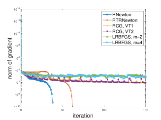
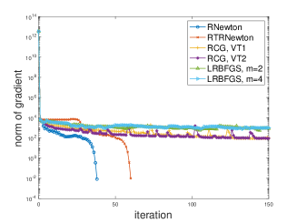
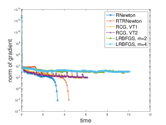
Figure 1: Compare RNewton, RTRNewton, RCG, and LRBFGS methods. For RCG, VT1 and VT2 respectively means that the vector transport is given vector transport by parallelization and by projection. For LRBFGS, $m$ means memory size.

We observe that all methods under consideration declined sharply at the beginning, which is due to the use of the proposed preconditioner (it will be discussed in detail later). Then both RCG and LRBFGS slowly decrease. RNewton and RTRNewton outperform the other two methods both in terms of the number of iterations and CPU time and they both exhibit superlinear convergence locally. While we note that RNewton is superior to RTRNewton in the number of iterations and CPU time. This shows the superiority of RNewton over other methods under consideration for solving Problem (3.2).

The Proposed Preconditioner v.s. the Preconditioner in [VV10].

We observe that from Table 1, after applying preconditioners, the number of inner iterations is significantly reduced, which greatly improves the efficiency of the algorithm. Since the proposed preconditioner is a generalization of the one in [VV10], we should expect that when the mass matrix $M=I$, the gain of applying the two preconditioners is coincident due to that the preconditioner [VV10] is derived under setting $M=I$. When $M\not=I$, due to that the preconditioner in [VV10] does not consider the structure of $M$, it can be expected that the efficiency of using the preconditioner in [VV10] is significantly lower than the efficiency of using the proposed preconditioner. These are verified by Table 1 and Table 2.

Table 1: Comparison of RNewton and RTRNewton on $\mathbb{R}_{*}^{n\times p}/\mathcal{O}_{p}$ for solving Problem (3.2) with data from Listing 1. There exist two choices for the mass matrix $M$: i) $M=I$ or ii) $M=\mathrm{diag}([\mathrm{rand}(n-1,1);0]+0.1)$. Algorithm stops if $\|\mathrm{grad}f(x_{i})\|/\|\mathrm{grad}f(x_{0})\|<10^{-12}$. Indices “iter” and “nH” denote the number of iterations and the number of action of Hessian evaluations, respectively. Besides, the number $a.bc_{-k}$ denotes $a.bc\times 10^{-k}$.

			RNewton			RTRNewton
			no precond.	proposed precond.	precond [VV10]	no precond	proposed precond.	precond. [VV10]
$M=I$	$n=4000$ $p=3$	iter	$3.80_{1}$	$3.00_{1}$	$3.10_{1}$	$6.70_{1}$	$5.50_{1}$	$5.50_{1}$
		nH	$8.01_{3}$	$5.50_{1}$	$5.60_{1}$	$7.68_{3}$	$1.30_{2}$	$1.30_{2}$
	$n=8000$ $p=5$	iter	$5.70_{1}$	$3.30_{1}$	$3.30_{1}$	$9.20_{1}$	$6.00_{1}$	$6.00_{1}$
		nH	$2.44_{4}$	$5.20_{1}$	$5.00_{1}$	$2.18_{4}$	$1.34_{2}$	$1.34_{2}$
	$n=20000$ $p=8$	iter	$7.00_{1}$	$3.60_{1}$	$3.80_{1}$	$9.60_{1}$	$5.80_{1}$	$6.00_{1}$
		nH	$2.96_{4}$	$5.60_{1}$	$5.70_{1}$	$2.53_{4}$	$1.26_{2}$	$1.29_{2}$
	$n=40000$ $p=10$	iter	$7.90_{1}$	$9.00$	$9.00$	$1.24_{2}$	$4.20_{1}$	$4.50_{1}$
		nH	$2.70_{4}$	$1.50_{1}$	$1.30_{1}$	$2.38_{4}$	$8.30_{1}$	$9.10_{1}$
$M\not=I$	$n=4000$ $p=3$	iter	$7.20_{1}$	$2.90_{1}$	$3.90_{1}$	$7.70_{1}$	$4.90_{1}$	$5.40_{1}$
		nH	$2.10_{4}$	$6.10_{1}$	$1.31_{2}$	$1.53_{4}$	$1.19_{2}$	$2.60_{2}$
	$n=8000$ $p=5$	iter	$1.07_{2}$	$4.00_{1}$	$4.40_{1}$	$1.22_{2}$	$5.90_{1}$	$6.40_{1}$
		nH	$4.01_{4}$	$8.90_{1}$	$1.56_{2}$	$3.65_{4}$	$1.47_{2}$	$3.04_{2}$
	$n=20000$ $p=8$	iter	$7.10_{1}$	$5.00_{1}$	$6.80_{1}$	$1.17_{2}$	$7.70_{1}$	$8.40_{1}$
		nH	$2.84_{4}$	$1.22_{2}$	$2.50_{2}$	$3.11_{4}$	$2.12_{2}$	$3.57_{2}$
	$n=40000$ $p=10$	iter	$7.40_{1}$	$2.00_{1}$	$6.30_{1}$	$1.38_{2}$	$5.00_{1}$	$6.20_{1}$
		nH	$2.86_{4}$	$4.40_{1}$	$2.27_{2}$	$1.66_{4}$	$1.25_{2}$	$2.41_{2}$

Quotient Manifold $\mathbb{R}_{*}^{n\times p}/\mathcal{O}_{p}$ v.s. Embedded Manifold $\mathcal{S}_{+}(p,n)$.

Applying the preconditioner proposed in Section 6.1, RNewton and RTRNewton have a remarkable advantage for solving Problem (3.2) over them for solving Problem (LABEL:Pro_stat-OptProb_Bart), which can be observed from Table 1 and Table 2, in terms of the number of iterations and the number of the actions of Hessian. Theoretically, the quotient manifold $\mathbb{R}_{*}^{n\times p}/\mathcal{O}_{p}$ is diffeomorphic to the embedded manifold $\mathcal{S}_{+}(p,n)$, but there exists significant difference lying in optimization. The main difference is the choice of retraction. For $\mathcal{S}_{+}(p,n)$, a projection-type retraction is used (see [VV10]), while an addition-type retraction (5.4) is used for $\mathbb{R}_{*}^{n\times p}/\mathcal{O}_{p}$. In most cases, the number of inner iterations (i.e., Algorithm 2 for quotient manifold) is very small, generally 0 or 1. That is, Algorithm 2 returns the approximate solution to Equation (6.2) with $-(\mathrm{grad}f(\pi(Y_{k})))_{\uparrow_{Y_{k}}}$ as the right-hand side. Specifically, the solution $\xi_{\uparrow_{Y_{k}}}$ satisfies

$$\left(I-\frac{1}{2}P_{Y_{k}}\right)\nabla^{2}h(Y_{k}Y_{k}^{T})[Y_{k}\xi_{\uparrow_{Y_{k}}}^{T}+\xi_{\uparrow_{Y_{k}}}Y_{k}^{T}]Y_{k}(Y_{k}^{T}Y_{k})^{-1}\approx-\left(I-\frac{1}{2}P_{Y_{k}}\right)\nabla h(Y_{k}Y_{k}^{T})Y_{k}(Y_{k}^{T}Y_{k})^{-1}.$$

This is equivalent to

$$(\nabla^{2}h(Y_{k}Y_{k}^{T})[Y_{k}\xi_{\uparrow_{Y_{k}}}^{T}+\xi_{\uparrow_{Y_{k}}}Y_{k}^{T}]+\nabla h(Y_{k}Y_{k}^{T}))Y_{k}\approx 0,$$

this is,

$$(A(Y_{k}\xi_{\uparrow_{Y_{k}}}^{T}+\xi_{\uparrow_{Y_{k}}}Y_{k}^{T}+Y_{k}Y_{k}^{T})M+M(Y_{k}\xi_{\uparrow_{Y_{k}}}^{T}+\xi_{\uparrow_{Y_{k}}}Y_{k}^{T}+YY^{T})A-C)Y_{k}\approx 0,$$

which implies

$$(A(Y_{k}+\xi_{\uparrow_{Y_{k}}})(Y_{k}+\xi_{\uparrow_{Y_{k}}})^{T}M+M(Y_{k}+\xi_{\uparrow_{Y_{k}}})(Y_{k}+\xi_{\uparrow_{Y_{k}}})^{T}A-C)Y_{k}\approx(A\xi_{\uparrow_{Y_{k}}}\xi_{\uparrow_{Y_{k}}}^{T}M+M\xi_{\uparrow_{Y_{k}}}\xi_{\uparrow_{Y_{k}}}^{T}A)Y_{k}.$$

For a randomly given initial guess $Y_{0}\in\mathbb{R}_{*}^{n\times p}$, we observe that $\|A\xi_{\uparrow_{Y_{k}}}\xi_{\uparrow_{Y_{k}}}^{T}M+M\xi_{\uparrow_{Y_{k}}}\xi_{\uparrow_{Y_{k}}}^{T}A\|_{F}$ is far less than $\|AY_{0}Y_{0}^{T}M+MY_{0}Y_{0}^{T}A-C\|_{F}$ from Table 3. That is to say, $Y+\eta_{\uparrow_{Y}}$ is a suitable candidate for the solution of (3.2) in the column space of $Y_{0}$. This also partly explains why it is better to define the problem on the quotient manifold $\mathbb{R}_{*}^{n\times p}/\mathcal{O}_{p}$ than on the embedded submanifold $\mathcal{S}_{+}(p,n)$.

Table 2: Comparisons of RNewton and RTRNewton on $\mathcal{S}_{+}(p,n)$ for solving Problem (LABEL:Pro_stat-OptProb_Bart) and on $\mathbb{R}_{*}^{n\times p}/\mathcal{O}_{p}$ for solving Problem (3.2) with data from Listing 1. The mass matrix is given by $M=\mathrm{diag}([\mathrm{rand}(n-1,1);0]+0.1)$. Algorithms stop if $\|\mathrm{grad}f(x_{i})\|/\|\mathrm{grad}f(x_{0})\|<10^{-11}$.

			RNewton		RTRNewton
			proposed precond.	precond. [VV10]	proposed precond.	precond. [VV10]
$\mathcal{S}_{+}(p,n)$	$n=20000$ $p=6$	iter	$6.90_{1}$	$9.30_{1}$	$1.21_{2}$	$1.41_{2}$
		nH	$1.38_{2}$	$2.89_{2}$	$2.57_{2}$	$4.27_{2}$
	$n=50000$ $p=12$	iter	$5.50_{1}$	$6.80_{1}$	$1.15_{2}$	$1.26_{2}$
		nH	$1.01_{2}$	$1.58_{2}$	$2.45_{2}$	$3.67_{2}$
	$n=80000$ $p=18$	iter	$6.50_{1}$	$1.04_{2}$	$1.04_{2}$	$1.23_{2}$
		nH	$8.50_{1}$	$2.08_{2}$	$2.11_{2}$	$3.57_{2}$
$\mathbb{R}_{*}^{n\times p}/\mathcal{O}_{p}$	$n=20000$ $p=6$	iter	$2.10_{1}$	$3.60_{1}$	$5.40_{1}$	$6.00_{1}$
		nH	$5.70_{1}$	$1.21_{2}$	$1.23_{2}$	$2.76_{2}$
	$n=50000$ $p=12$	iter	$4.00$	$1.70_{1}$	$4.10_{1}$	$4.10_{1}$
		nH	$6.00$	$4.90_{1}$	$8.20_{1}$	$1.39_{2}$
	$n=80000$ $p=18$	iter	$2.00$	$1.20_{1}$	$3.70_{1}$	$3.70_{1}$
		nH	$2.00$	$4.20_{1}$	$7.30_{1}$	$1.88_{2}$

Table 3: The data and the parameters are the same as Table 1. Here approx_res = $\|A\xi_{\uparrow_{Y_{k}}}\xi_{\uparrow_{Y_{k}}}^{T}M+M\xi_{\uparrow_{Y_{k}}}\xi_{\uparrow_{Y_{k}}}^{T}A\|_{F}/\|AY_{0}Y_{0}^{T}+MY_{0}Y_{0}^{T}A-C\|_{F}$.

			RNewton		RTRNewton
			proposed precond.	precond. [VV10]	proposed precond.	precond. [VV10]
$\mathcal{S}_{+}(p,n)$	$(n,p)=(20000,6)$	approx_res	$2.32_{-12}$	$4.32_{-14}$	$8.26_{-12}$	$4.12_{-14}$
	$(n,p)=(50000,12)$	approx_res	$3.34_{-7}$	$1.13_{-10}$	$3.09_{-11}$	$8.11_{-11}$
	$(n,p)=(80000,18)$	approx_res	$8.07_{-9}$	$1.95_{-11}$	$8.39_{-11}$	$1.30_{-11}$

7.3 Comparison with Existing Low-Rank Methods

In this section, Algorithm 4, called IRRLayp, is compared with three existing state-of-the-art low-rank methods for Lyapunov equations, including K-PIK from [Sim07], RKSM from [DS11, KS20], and mess_lradi from a Matlab toolbox named M-M.E.S.S [SKB22]. These methods are respectively based on Krylov subspace techniques (K-PIK, RKSM), and alternating direction implicit iterative (mess_lradi). For mess_lradi, there are three methods for selecting shifts, “heuristic”, “wachspress”, and “projection”, which are all tested in our experiments. Since, in Algorithm 4, other Riemannian methods can be used to solve the subproblem, we further use the Riemannian trust-region Newton’s method in [ABG07] and the resulting algorithm is denoted by IRRLyap-RTRNewton. Algorithm 4 combined with Algorithm 1 is denoted by IRRLyap-RNewton. As a reference, the notation “best low rank” with rank $p$ denotes a best low-rank approximation by the truncated singular value decomposition to the exact solution of (1.1).

Quality of low-rank solutions.

The generalized Lyapunov equation was drawn from a RAIL benchmark problem with the coefficient matrix of size $n=1357$. For the sake of simplicity, the right-hand side is taken as $C=B(:,1)B(:,1)^{T}$. Figure 2 shows the experiment results.

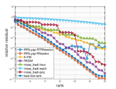
Figure 2: The relative residual for one-rank right-hand-side RAIL benchmark with $n=1357$.

It can be seen from Figure 2 that under the same rank, the relative residuals of the low-rank approximations from K-PIK and mess_lradi are notably greater than those from “best low rank”. Therefore, mess_lradi and K-PIK are not preferred if lower-rank solutions are desired. In addition, selecting shifts method by projection performs best for mess_lradi. When the relative residual is greater than $10^{-6}$, that is, highly accurate solutions are not needed, the solutions from IRRLyap-RTRNewton and IRRLyap-RNewton are close in the sense of the relative residual. This is because IRRLyap-RTRNewton and IRRLyap-RNewton solve the same optimization problem. However, when the relative residual is smaller than $10^{-6}$, the relative residuals from IRRLyap-RTRNewton begin to fluctuate without falling. We find that for this problem, RTRNewton is more sensitive to numerical error than RNewton in the sense that RTRNewon sometimes terminates before reaching the stopping criterion. Such behavior of RTRNewton prevents it from finding highly accurate solutions. Therefore, we conclude that IRRLyap-RNewton is preferable compared to IRRLyap-RTRNewton. The solutions found by IRRLyap-RNewton and RKSM are close to the ones by “best low rank”. IRRLyap-RNewton even have smaller relative residuals than those from “best low rank”. This is not surprising since “best low rank” uses truncated SVD and completely ignore the original problem whereas IRRLyap-RNewton aims to find a stationary point, i.e., minimizes the Riemannian gradient—the residual in the horizontal space, see Proposition 5.1. Overall, IRRLyap-RNewton is able to find the best solution compared to the tested methods in the sense of the relative residual.

Efficiency and performance.

K-PIK, RKSM, mess_lradi, IRRLyap-RNewton, and lradi-RNewton (i.e., mess_lradi provides a coarse solution that is used to be an initial guess of RNewton) are compared by using the RAIL benchmark problems with size $n=5177,20209,79841$. The stopping criterion for all methods are unified as $\|R\|_{F}=\|AXM+MXA-C\|_{F}\leq\tau\cdot\|C\|_{F}$ with a tolerance $\tau=10^{-6}$. The results are reported in Table 4.

Table 4: Comparison for the simplified RAIL benchmark with existing methods. “rank”, “time”, “rel_res”, “numSys”, and “timeSys” respectively denote the rank of the approximation, running time, the relative residual of the approximation, the number of solving shift systems $(A+\lambda M)X=b$ for $X$ with given $A,\lambda,M$ and $b$ (column vector or matrix, the numbers in parentheses indicate the number of matrices), and the CPU time for solving all those shift systems. Besides, the number $a.bc_{-k}$ denotes $a.bc\times 10^{-k}$.

	rannk	time(s.)	rel_res	numSys	timeSys	rannk	time(s.)	rel_res	numSys	timeSys	rannk	time(s.)	rel_res	numSys	timeSys
	5177					20209					79841
K-PIK	126	$4.61$	$1.46_{-6}$	64	$1.44$	182	$4.78_{1}$	$2.65_{-6}$	92	$7.47$	248	$5.34_{2}$	$4.39_{-6}$	125	$6.36_{1}$
RKSM	27	$1.94$	$7.07_{-7}$	28	$1.67_{-1}$	38	$2.66_{1}$	$2.65_{-6}$	39	$1.31$	41	$2.70_{2}$	$4.39_{-6}$	42	$7.79$
mess_lradi	32	$3.58_{-1}$	$1.47_{-7}$	64		37	$1.12$	$5.90_{-7}$	74		38	$4.14$	$6.12_{-8}$	76
lradi-RNewton	26	$2.37$	$6.31_{-7}$	8268(156)	$1.29$	32	$7.56$	$2.28_{-7}$	6240(96)	$4.61$	32	$7.26_{1}$	$4.13_{-6}$	14560(224)	$4.67_{1}$
IRRlyap-RNewton	22	$5.78$	$7.12_{-7}$	16095(521)	$3.51$	27	$4.44_{1}$	$3.29_{-7}$	28410(822)	$3.04_{1}$	27	$2.71_{2}$	$5.21_{-7}$	36950(1038)	$1.79_{2}$

For the three Lyapunov equations, K-PIK fails to satisfy the stopping criterion, implying that K-PIK has difficulty finding highly accurate solutions. Moreover, K-PIK needs to use a higher rank to reach a similar residual compared to other methods. Therefore, K-PIK is not preferred. The method mess_lradi is the most efficient algorithm in the sense of computational time. However, it also requires a higher rank for similar accuracy when compared to lradi_RNewton and IRRLyap-RNewton. Thus, mess_lradi is preferred if one has strict requirements on efficiency but not on rank. In view of this, noting the fact that mess_lradi can rapid provides a coarse solution and the fact that RNewton can refine the coarse solution, we integrate mess_lradi with RNewton. The resulting method, lradi_RNewton, requires a relative lower rank for similar accuracy while reduces significantly computational time. Additionally, the method RKSM also requires a higher rank for similar accuracy compared to IRRLya-RNewton, and for two medium to large-scale problems, it seems to be difficult to find highly accurate solutions. However, the proposed method IRRLyap-RNewton gives the solutions with lowest rank compared to the rest methods. We can observe from Table 4 that most of the time in lradi_RNewton and IRRLyap-RNewton are taken to solve the shift systems. Therefore, for some problems, if the resulting shift systems can be solved more efficiently, then the efficiency of lradi_RNewton and IRRLyap-RNewton can be further improved. Overall, we suggest using IRRLyap-RNewton if one does not have strict restrictions on computational time and desires as low-rank solutions as possible.

8 Conclusions

In this paper, we have generalized the truncated Newton’s method from Euclidean spaces to Riemannian manifolds, called Riemannian truncated-Newton’s method, and shown the convergence results, e.g., global convergence and local superlinear convergence. Moreover, the cost function from [VV10] is reformulated as an optimization problem defined on the Riemannian quotient manifold $\mathbb{R}^{n\times p}/\mathcal{O}_{p}$. An algorithm, called IRRLyap-RNewton, is proposed and is used to find a low-rank approximation of the generalized Lyapunov equations. We develop a new preconditioner that take $M\neq I$ into consideration. The numerical results show that the proposed RNewton has superior advangate over RTRNewton, RCG, and LRBGFS for solving Problem (3.2), and that the new preconditioner significantly reduce the number of actions of Riemannian Hessian evaluations even when $M\neq I$. In addition, IRRLyap-RNewton is able to find a similar accurate solution with the lowest rank compared to some state-of-the-art methods, including K-PIK, and mess_lradi.

Appendix A Appendix

A.1 The Other Two Metrics and Corresponding Preconditioners.

Riemannian metrics on $\mathbb{R}_{*}^{n\times p}$.

Two other Riemannian metrics on $\mathbb{R}_{*}^{n\times p}$ given in [ZHVZ23] also are considered here:

$$g^{i}_{Y}(\eta_{Y},\xi_{Y})=\begin{cases}\mathrm{tr}(Y^{T}Y\eta_{Y}^{T}\xi_{Y})&i=2,\\ \mathrm{tr}(\eta_{Y}^{T}\xi_{Y})&i=3,\end{cases}$$ (A.1)

the Riemannian metric $g_{Y}^{2}$ has been used in [HGZ17], where the space under consideration is on the complex field; and the Riemannian metric $g_{Y}^{3}$ is the standard Euclidean inner product on $\mathbb{R}^{n\times p}$ and has been considered in [MA20].

Horizontal spaces.

Given a Riemannian metric $g$ on the total space $\mathbb{R}_{*}^{n\times p}$, the orthogonal complement space in $\mathrm{T}_{Y}\mathbb{R}_{*}^{n\times p}$ of $\mathrm{V}_{Y}$ with respect to $g_{Y}$ is called the horizontal space at $Y$, denoted by $\mathrm{H}_{Y}$. The horizontal spaces with respect to the three Riemannian metrics in (A.1) are respectively given by

$$\mathrm{H}_{Y}^{i}=\begin{cases}\{YS+Y_{\perp}K:S^{T}=S,S\in\mathrm{R}^{p\times p},K\in\mathbb{R}^{(n-p)\times p}\}&i=2,\\ \{Y(Y^{T}Y)^{-1}S+Y_{\perp}K:S^{T}=S,S\in\mathbb{R}^{p\times p},K\in\mathbb{R}^{(n-p)\times p}\}&i=3.\end{cases}$$

Projections onto Vertical Spaces and Horizontal Spaces.

For any $Y\in\mathbb{R}_{*}^{n\times p}$ and $\eta_{Y}\in\mathrm{T}_{Y}\mathbb{R}_{*}^{n\times p}$, the orthogonal projections of $\eta_{Y}$ to $\mathrm{V}_{Y}$ and $\mathrm{H}_{Y}^{i}$ with respect to the second metric are respectively given by

$$\mathcal{P}_{Y}^{\mathrm{V}^{2}}(\eta_{Y})=Y\Omega,\text{ and }\mathcal{P}_{Y}^{\mathrm{H}^{2}}(\eta_{Y}) =\eta_{Y}-\mathcal{P}_{Y}^{\mathrm{V}^{2}}(\eta_{Y})=\eta_{Y}-Y\Omega$$

$$=Y\left(\frac{(Y^{T}Y)^{-1}Y^{T}\eta_{Y}+\eta_{Y}^{T}Y(Y^{T}Y)^{-1}}{2}\right)+Y_{\perp}Y_{\perp}^{T}\eta_{Y},$$

where $\Omega=\frac{(Y^{T}Y)^{-1}Y^{T}\eta_{Y}-\eta_{Y}^{T}Y(Y^{T}Y)^{-1}}{2}$. The orthogonal projections to vertical and horizontal spaces with respect to the third metric are

$$\mathcal{P}_{Y}^{\mathrm{V}^{3}}(\eta_{Y})=Y\Omega,\text{ and }\mathcal{P}_{Y}^{\mathrm{H}^{3}}(\eta_{Y})=\eta_{Y}-\mathcal{P}_{Y}^{\mathrm{V}^{3}}(\eta_{Y})=\eta_{Y}-Y\Omega,$$

where $\Omega$ is the skew-symmetric matrix satisfying $\Omega Y^{T}Y+Y^{T}Y\Omega=Y^{T}\eta_{Y}-\eta^{T}_{Y}Y.$

Riemannian metrics on $\mathbb{R}_{*}^{n\times p}/\mathcal{O}_{p}$.

Since the two Riemannian metrics $g_{Y}^{2},g_{Y}^{3}$ on $\mathbb{R}_{*}^{n\times p}$ satisfy (5.2) by [ZHVZ23], the corresponding three metrics on $\mathbb{R}_{*}^{n\times p}/\mathcal{O}_{p}$ are given by:

$$g^{i}_{\pi(Y)}(\xi_{\pi(Y)},\eta_{\pi(Y)})= \mathrm{tr}(Y^{T}Y\xi_{\uparrow_{Y}}^{T}\eta_{\uparrow_{Y}}) i=2,$$ (A.2a)

$$g^{i}_{\pi(Y)}(\xi_{\pi(Y)},\eta_{\pi(Y)})= \mathrm{tr}(\xi_{\uparrow_{Y}}^{T}\eta_{\uparrow_{Y}}) i=3,$$ (A.2b)

for all $\xi_{\pi(Y)},\eta_{\pi(Y)}\in\mathrm{T}_{\pi(Y)}\mathbb{R}_{*}^{n\times p}/\mathcal{O}_{p}$. In the following, with a slight abuse of notation, we use $g^{i}$, $i=2,3$, to denote the Riemannian metrics on both $\mathbb{R}_{*}^{n\times p}$ and $\mathbb{R}_{*}^{n\times p}/\mathcal{O}_{p}$.

The horizontal lifts of Riemannian Gradients and the actions of Riemannian Hessians.

It follows from [ZHVZ23] that the Riemannian gradients and Riemannian Hessian of $f$ in (3.2) can be characterized by the Euclidean gradient and the Euclidean Hessian of $h$ in (LABEL:Pro_stat-OptProb_Bart), see Proposition 5.1.

Proposition A.1.

The Riemannian gradients of the smooth real-valued function $f$ in (3.2) on $\mathbb{R}_{*}^{n\times p}/\mathcal{O}_{p}$ with respect to the two other Riemannian metrics are respectively given by

$$(\mathrm{grad}f(\pi(Y)))_{\uparrow_{Y}}=\mathrm{grad}\bar{f}(Y)=\begin{cases}2\nabla h(YY^{T})Y(Y^{T}Y)^{-1}&\text{ under metric }g^{2},\\ 2\nabla h(YY^{T})Y&\text{ under metric }g^{3},\end{cases}$$

and the actions of the Riemannian Hessians are respectively given by

$$(\mathrm{Hess}f(\pi(Y))[\eta_{\pi(Y)}])_{\uparrow_{Y}}= 2\nabla^{2}h(YY^{T})[Y\eta_{\uparrow_{Y}}^{T}+\eta_{\uparrow_{Y}}Y^{T}]Y(Y^{T}Y)^{-1}+T_{2} i=2,$$ (A.3a)

$$(\mathrm{Hess}f(\pi(Y))[\eta_{\pi(Y)}])_{\uparrow_{Y}}= 2\nabla^{2}h(YY^{T})[Y\eta_{\uparrow_{Y}}^{T}+\eta_{\uparrow_{Y}}Y^{T}]Y+T_{3} i=3,$$ (A.3b)

where $\nabla^{2}h(YY^{T})[V]=AVM+MVA$, $P_{Y}=Y(Y^{T}Y)^{-1}Y^{T}$, $T_{2}=\mathcal{P}_{Y}^{\mathrm{H}^{2}}\{\nabla h(YY^{T})P_{Y}^{\perp}\eta_{\uparrow_{Y}}(Y^{T}Y)^{-1}+P_{Y}^{\perp}\nabla h(YY^{T})\eta_{\uparrow_{Y}}(Y^{T}Y)^{-1}+2\mathrm{skew}(\eta_{\uparrow_{Y}}Y^{T})\nabla h(YY^{T})Y(Y^{T}Y)^{-2}+2\mathrm{skew}\{\eta_{\uparrow_{Y}}(Y^{T}Y)^{-1}Y^{T}\nabla h(YY^{T})\}Y(Y^{T}Y)^{-1}\}$, and $T_{3}=2\mathcal{P}_{Y}^{\mathrm{H}^{3}}\{\nabla h(YY^{T})\eta_{\uparrow_{Y}}\}$.

A.2 Preconditioning under Riemannian Metrics (A.2a) and (A.2b)

Similar to the approach in Section 6.1, the preconditioners for Riemannian metrics (A.2a) and (A.2b) respectively solves the equations

$$[A(Y\xi_{\uparrow_{Y}}^{T}+\xi_{\uparrow_{Y}}Y^{T})M+M(Y\xi_{\uparrow_{Y}}^{T}+\xi_{\uparrow_{Y}}Y^{T})A]Y=\eta_{\uparrow_{Y}}(Y^{T}Y),\hbox{ for $\xi_{\uparrow_{Y}}\in\mathrm{H}_{Y}^{2}$ }$$ (A.4)

and

$$2[A(Y\xi_{\uparrow_{Y}}^{T}+\xi_{\uparrow_{Y}}Y^{T})M+M(Y\xi_{\uparrow_{Y}}^{T}+\xi_{\uparrow_{Y}}Y^{T})A]Y=\eta_{\uparrow_{Y}},\hbox{ for $\xi_{\uparrow_{Y}}\in\mathrm{H}_{Y}^{3}$}.$$ (A.5)

The derivations are analogous to those in Section 6.1 and therefore are not repeated here. The algorithms for solving (A.4) and (A.4) are respectively stated in Algorithm 5 and Algorithm 6. Note that in Step 9 and 10 of Algorithm 6, two small-scale Sylvester equations of size $p\times p$ need be solved and can be done by using lyap function in MATLAB.

Algorithm 5 Preconditioner under Riemannian metric (A.2a)

0:  Matrices $A$ and $M$ and horizontal vector $\eta_{\uparrow_{Y}}\in\mathrm{H}_{Y}^{2}$;

0:  $\xi_{\uparrow_{Y}}$ satisfying (A.4);

1:  Set $LL^{T}\leftarrow Y^{T}MY$ (Cholesky factorization);

2:  Set $Q\Lambda Q^{T}\leftarrow L^{-1}Y^{T}AYL^{-T}$ (Eigenvalues decomposition);

3:  Set $\hat{V}\leftarrow\mathrm{orthonormal}(MY)$;

4:  Set $v_{i}\leftarrow Q^{T}L^{-1}Y^{T}A\mathcal{T}_{i}^{-1}\left((I-\hat{V}\hat{V}^{T})\frac{1}{2}\eta_{\uparrow_{Y}}(Y^{T}Y)L^{-T}Q(:,i)\right)$;

5:  Set $K_{i}\leftarrow 2\lambda_{i}I-Q^{T}L^{-1}Y^{T}A\mathcal{T}_{i}^{-1}\left((I-\hat{V}\hat{V}^{T})2AYL^{-T}Q\right)$;

6:  Set $R\leftarrow\frac{1}{2}Q^{T}L^{-1}Y^{T}\eta_{\uparrow_{Y}}(Y^{T}Y)L^{-T}Q-[v_{1},\cdots,v_{k}]-[v_{1},\cdots,v_{k}]^{T}$;

7:  Solve for $\tilde{S}_{\xi}$ by $(\mathcal{K}+\Pi\mathcal{K}\Pi)\mathrm{vec}(\tilde{S}_{\xi})=\mathrm{vec}(R)$;

8:  Solve for $\tilde{Z}_{\xi}$ by

$$\tilde{Z}_{\xi}(:,i)\leftarrow\mathcal{T}_{i}^{-1}\left((I-\hat{V}\hat{V}^{T})\frac{1}{2}\eta_{\uparrow_{Y}}(Y^{T}Y)L^{-1}Q(:,i)\right)-\mathcal{T}_{i}^{-1}\left((I-\hat{V}\hat{V}^{T})2AYL^{-T}Q\right)\tilde{S}_{\xi}(:,i);$$

9:  Set $Z_{\xi,1}\leftarrow\frac{1}{2}Y\left((Y^{T}Y)^{-1}Y^{T}\tilde{Z}_{\xi}Q^{T}L^{-1}+L^{-T}Q\tilde{Z}_{\xi}^{T}Y(Y^{T}Y)^{-1}\right)$;

10:  Set $Z_{\xi,2}\leftarrow(I-Y(Y^{T}Y)^{-1}Y^{T}\tilde{Z}_{\xi}Q^{T}L^{-1}$;

11:  Set $\xi_{\uparrow_{Y}}\leftarrow YL^{-T}Q\tilde{S}_{\xi}Q^{T}L^{-1}+Z_{\xi,1}+Z_{\xi,2}$.

Algorithm 6 Preconditioner under Riemannian metric (A.2b)

0:  Matrices $A$ and $M$ and horizontal vector $\eta_{\uparrow_{Y}}\in\mathrm{H}_{Y}^{3}$;

0:  $\xi_{\uparrow_{Y}}$ satisfying (A.5);

1:  Set $LL^{T}\leftarrow Y^{T}MY$ (Cholesky factorization);

2:  Set $Q\Lambda Q^{T}\leftarrow L^{-1}Y^{T}AYL^{-T}$ (Eigenvalues decomposition);

3:  Set $\hat{V}\leftarrow\mathrm{orthonormal}(MY)$;

4:  Set $v_{i}\leftarrow Q^{T}L^{-1}Y^{T}A\mathcal{T}_{i}^{-1}\left((I-\hat{V}\hat{V}^{T})\frac{1}{2}\eta_{\uparrow_{Y}}L^{-T}Q(:,i)\right)$;

5:  Set $K_{i}\leftarrow 2\lambda_{i}I-Q^{T}L^{-1}Y^{T}A\mathcal{T}_{i}^{-1}\left((I-\hat{V}\hat{V}^{T})2AYL^{-T}Q\right)$;

6:  Set $R\leftarrow\frac{1}{2}Q^{T}L^{-1}Y^{T}\eta_{\uparrow_{Y}}L^{-T}Q-[v_{1},\cdots,v_{k}]-[v_{1},\cdots,v_{k}]^{T}$;

7:  Solve for $\tilde{S}_{\xi}$ by $(\mathcal{K}+\Pi\mathcal{K}\Pi)\mathrm{vec}(\tilde{S}_{\xi})=\mathrm{vec}(R)$;

8:  Solve for $\tilde{Z}_{\xi}$ by

$$\tilde{Z}_{\xi}(:,i)\leftarrow\mathcal{T}_{i}^{-1}\left((I-\hat{V}\hat{V}^{T})\frac{1}{2}\eta_{\uparrow_{Y}}L^{-1}Q(:,i)\right)-\mathcal{T}_{i}^{-1}\left((I-\hat{V}\hat{V}^{T})2AYL^{-T}Q\right)\tilde{S}_{\xi}(:,i);$$

9:  Solve for $S_{\xi}$ by $S_{\xi}(Y^{T}Y)^{-1}+(Y^{T}Y)^{-1}S_{\xi}=2L^{-T}Q\tilde{S}_{\xi}Q^{T}L^{-1}$;

10:  Solve for $\Omega$ by $\Omega Y^{T}Y+Y^{T}Y\Omega=Y^{T}\tilde{Z}_{\xi}Q^{T}L^{-1}-L^{-T}Q\tilde{Z}_{\xi}^{T}Y$;

11:  Set $\xi_{\uparrow_{Y}}\leftarrow Y(Y^{T}Y)^{-1}S_{\xi}+\tilde{Z}_{\xi}Q^{T}L^{-1}-Y\Omega$.

References

- [ABG07] P.-A. Absil, C.G. Baker, and K.A. Gallivan. Trust-region methods on Riemannian manifolds. Foundations of Computational Mathematics, 7:303–330, 2007.
- [AMS08] P.-A. Absil, Robert Mahony, and Rodolphe Sepulchre. Optimization algorithms on matrix manifolds. Princeton University Press, 2008.
- [Ant05] Athanasios C. Antoulas. Approximation of large-scale dynamical systems. In Advances in Design and Control, 2005.
- [BA15] Nicolas Boumal and Pierre-Antoine Absil. Low-rank matrix completion via preconditioned optimization on the grassmann manifold. Linear Algebra and its Applications, 475:200–239, 2015.
- [Bau08] Ulrike Baur. Low rank solution of data-sparse Sylvester equations. Numerical Linear Algebra with Applications, 15:837–851, 2008.
- [BB06] Ulrike Baur and Peter Benner. Factorized solution of Lyapunov equations based on hierarchical matrix arithmetic. Computing, 78(3):211–234, 2006.
- [BGL05] Michele Benzi, Gene H. Golub, and Jörg Liesen. Numerical solution of saddle point problems. Acta Numerica, 14:1–137, 2005.
- [BHW21] Peter Benner, Jan Heiland, and Steffen W. R. Werner. A low-rank solution method for Riccati equations with indefinite quadratic terms. Numerical Algorithms, 92:1083–1103, 2021.
- [BK14] Peter Benner and Patrick Kürschner. Computing real low-rank solutions of Sylvester equations by the factored ADI method. Computers and Mathematics with Applications, 67(9):1656–1672, 2014.
- [BLT09] Peter Benner, Ren-Cang Li, and Ninoslav Truhar. On the ADI method for Sylvester equations. Journal of Computational and Applied Mathematics, 233(4):1035–1045, 2009.
- [BM03] Samuel Burer and Renato D.C. Monteiro. A nonlinear programming algorithm for solving semidefinite programs via low-rank factorization. Mathematical Programming, 95(2):329–357, 2003.
- [BN89] Richard H. Byrd and Jorge Nocedal. A tool for the analysis of quasi-Newton methods with application to unconstrained minimization. SIAM Journal on Numerical Analysis, 26:727–739, 1989.
- [Boo75] W. M. Boothby. In An introduction to differentiable manifolds and Riemannian geometry, volume 63 of Pure and Applied Mathematics. Elsevier, 1975.
- [Bou20] Nicolas Boumal. An introduction to optimization on smooth manifolds. Cambridge University Press, 2020.
- [BPS22] Peter Benner, Davide Palitta, and Jens Saak. On an integrated Krylov-ADI solver for large-scale Lyapunov equations. Numerical Algorithms, 92(1):35–63, 2022.
- [BS72] R. H. Bartels and G. W. Stewart. Algorithm 432 [c2]: Solution of the matrix equation AX + XB = C [f4]. Communications of the ACM, 15(9):820–826, 1972.
- [BS05] Peter Benner and Jens Saak. A semi-discretized heat transfer model for optimal cooling of steel profiles. In Dimension Reduction of Large-Scale Systems, pages 353–356. Springer Berlin Heidelberg, 2005.
- [Chu87] King-wah Eric Chu. The solution of the matrix equations AXB-CXD=E and (YA-DZ,YC-BZ)=(E,F). Linear Algebra and its Applications, 93:93–105, 1987.
- [dABFF22] Márcio Antônio de Andrade Bortoloti, Teles A. Fernandes, and Orizon Pereira Ferreira. An efficient damped Newton-type algorithm with globalization strategy on Riemannian manifolds. Journal of Computational and Applied Mathematics, 403(3):113853, 2022.
- [dABFFY18] Márcio Antônio de Andrade Bortoloti, Teles A. Fernandes, Orizon Pereira Ferreira, and Jinyun Yuan. Damped Newton’s method on Riemannian manifolds. Journal of Global Optimization, 77(3):643–660, 2018.
- [DES82] Ron S. Dembo, Stanley C. Eisenstat, and Trond Steihaug. Inexact Newton methods. SIAM Journal on Numerical Analysis, 19(2):400–408, 1982.
- [DS83a] Ron S. Dembo and Trond Steihaug. Truncated-Newton algorithms for large-scale unconstrained optimization. Mathematical Programming, 26(2):190–212, 1983.
- [DS83b] John E. Dennis and Bobby Schnabel. Numerical methods for unconstrained optimization and nonlinear equations. In Prentice Hall series in computational mathematics, 1983.
- [DS11] Vladimir Druskin and Valeria Simoncini. Adaptive rational Krylov subspaces for large-scale dynamical systems. Systems and Control Letters, 60:546–560, 2011.
- [GDA+20] Bhawna Goyal, Ayush Dogra, Sunil Agrawal, B. S. Sohi, and Apoorav Sharma. Image denoising review: From classical to state-of-the-art approaches. Information Fusion, 55:220–244, 2020.
- [GGB22] Ion Victor Gosea, Serkan Gugercin, and Christopher Beattie. Data-driven balancing of linear dynamical systems. SIAM Journal on Scientific Computing, 44(1):A554–A582, 2022.
- [GL96] Gene H. Golub and Charles Van Loan. In Matrix computations (3rd ed.), 1996.
- [GNVL79] G. Golub, S. Nash, and C. Van Loan. A Hessenberg-Schur method for the problem AX + XB= C. IEEE Transactions on Automatic Control, 24(6):909–913, 1979.
- [Gra04] Lars Grasedyck. Existence of a low rank or H-matrix approximant to the solution of a Sylvester equation. Numerical Linear Algebra with Applications, 11:371–389, 2004.
- [GSA03] S. Gugercin, D.C. Sorensen, and A.C. Antoulas. A modified low-rank Smith method for large-scale Lyapunov equations. Numerical Algorithms, 32(1):27–55, 2003.
- [HAG15] Wen Huang, Pierre-Antoine Absil, and Kyle A. Gallivan. A Riemannian symmetric rank-one trust-region method. Mathematical Programming, 150:179–216, 2015.
- [HAG18] Wen Huang, P.-A. Absil, and K. A. Gallivan. A Riemannian BFGS method without differentiated retraction for nonconvex optimization pproblems. SIAM Journal on Optimization, 28(1):470–495, 2018.
- [HAGH18] Wen Huang, P.-A. Absil, Kyle A. Gallivan, and Paul Hand. ROPTLIB: An object-oriented C++ library for optimization on Riemannian manifolds. ACM Transactions on Mathematical Software, 44(4), jul 2018.
- [Ham82] S. J. Hammarling. Numerical solution of the stable, non-negative definite Lyapunov equation. SIMA Journal of Numerical Analysis, 2(3):303–323, 07 1982.
- [HG22] Wen Huang and Kyle A. Gallivan. A limited-memory Riemannian symmetric rank-one trust-region method with a restart strategy. Journal of Scientific Computing, 93(1), 2022.
- [HGA15] Wen Huang, Kyle A. Gallivan, and Pierre-Antoine Absil. A Broyden class of quasi-Newton methods for Riemannian optimization. SIAM Journal on Optimization, 25:1660–1685, 2015.
- [HGZ17] Wen Huang, K. A. Gallivan, and Xiangxiong Zhang. Solving PhaseLift by low-rank Riemannian optimization methods for complex semidefinite constraints. SIAM Journal on Scientific Computing, 39(5):B840–B859, 2017.
- [HJR21] Majed Hamadi, Khalide Jbilou, and Ahmed Ratnani. A model reduction method in large scale dynamical systems using an extended-rational block Arnoldi method. Journal of Applied Mathematics and Computing, 68:271–293, 2021.
- [HS52] Magnus R. Hestenes and Eduard Stiefel. Methods of conjugate gradients for solving linear systems. Journal of research of the National Bureau of Standards, 49:409–435, 1952.
- [HS95] Uwe Helmke and Mark A. Shayman. Critical points of matrix least squares distance functions. Linear Algebra and its Applications, 215:1–19, 1995.
- [IP18] Bruno Iannazzo and Margherita Porcelli. The Riemannian Barzilai–Borwein method with nonmonotone line search and the matrix geometric mean computation. Ima Journal of Numerical Analysis, 38:495–517, 2018.
- [J9́6] Lucas Jódar. Lyapunov matrix equation in system stability and control (Zoran Gajic and Muhammad Tahir Javed Qureshi). SIAM Review, 38(4):691–691, 1996.
- [KS20] Gerhard Kirsten and Valeria Simoncini. Order reduction methods for solving large-scale differential matrix riccati equations. SIAM Journal on Scientific Computing, 42(4):A2182–A2205, 2020.
- [Loa00] Charles F.Van Loan. The ubiquitous Kronecker product. Journal of Computational and Applied Mathematics, 123(1):85–100, 2000.
- [LW04] Jing-Rebecca Li and Jacob White. Low-rank solution of Lyapunov equations. SIAM Review, 46(4):693–713, 2004.
- [MA20] Estelle Massart and P.-A. Absil. Quotient geometry with simple geodesics for the manifold of fixed-rank positive-semidefinite matrices. SIAM Journal on Matrix Analysis and Applications, 41(1):171–198, 2020.
- [Moo81] Bradley Alan Moore. Principal component analysis in linear systems: Controllability, observability, and model reduction. IEEE Transactions on Automatic Control, 26:17–32, 1981.
- [MV14] B. Mishra and B. Vandereycken. A Riemannian approach to low-rank algebraic Riccati equations, 2014.
- [NW06] Jorge Nocedal and Stephen J. Wright. Numerical optimization. Springer series in operations research. Springer, 2nd ed edition, 2006.
- [Pen98] Thilo Penzl. Numerical solution of generalized Lyapunov equations. Advances in Computational Mathematics, 8(1):33–48, 1998.
- [Pen00] Thilo Penzl. Eigenvalue decay bounds for solutions of Lyapunov equations: the symmetric case. Systems and Control Letters, 40(2):139–144, 2000.
- [PS16] Davide Palitta and Valeria Simoncini. Matrix-equation-based strategies for convection–diffusion equations. BIT Numerical Mathematics, 56(2):751–776, 2016.
- [RW12] Wolfgang Ring and Benedikt Wirth. Optimization methods on Riemannian manifolds and their application to shape space. SIAM Journal on Optimization, 22(2):596–627, 2012.
- [Sat16] Hiroyuki Sato. A Dai–Yuan-type Riemannian conjugate gradient method with the weak wolfe conditions. Computational Optimization and Applications, 64(1):101–118, 2016.
- [SB04] Jens Saak and Peter Benner. Efficient numerical solution of the LQR-problem for the heat equation. Proceedings in Applied Mathematics and Mechanics, 4(1), 2004.
- [SI15] Hiroyuki Sato and Toshihiro Iwai. A new, globally convergent Riemannian conjugate gradient method. Optimization, 64(4):1011–1031, 2015.
- [Sim07] V. Simoncini. A new iterative method for solving large-scale Lyapunov matrix equations. SIAM Journal on Scientific Computing, 29(3):1268–1288, 2007.
- [SKB22] J. Saak, M. Köhler, and P. Benner. M-M.E.S.S.-2.1 – the matrix equations sparse solvers library, February 2022. see also: https://www.mpi-magdeburg.mpg.de/projects/mess.
- [SVdVR08] Wil Schilders, Henk Van der Vorst, and Joost Rommes. volume 13. Springer, 2008.
- [VV10] Bart Vandereycken and Stefan Vandewalle. A Riemannian optimization approach for computing low-rank solutions of Lyapunov equations. SIAM Journal on Matrix Analysis and Applications, 31(5):2553–2579, 2010.
- [WZB20] Yang Wang, Zhi Zhao, and Zhengjian Bai. Riemannian Newton-CG methods for constructing a positive doubly stochastic matrix from spectral data*. Inverse Problems, 36(11):115006, 2020.
- [ZBJ18] Zhi Zhao, Zhengjian Bai, and Xiaoqing Jin. A Riemannian inexact Newton-CG method for constructing a nonnegative matrix with prescribed realizable spectrum. Numerische Mathematik, 140:827–855, 2018.
- [Zhu17] Xiaojing Zhu. A Riemannian conjugate gradient method for optimization on the Stiefel manifold. Computational Optimization and Applications, 67:73–110, 2017.
- [ZHVZ23] Shixin Zheng, Wen Huang, Bart Vandereycken, and Xiangxiong Zhang. Riemannian optimization using three different metrics for hermitian PSD fixed-rank constraints: an extended version, 2023.