Randomization Inference of Heterogeneous Treatment Effects under Network Interference

Abstract

We design randomization tests of heterogeneous treatment effects when units interact on a single connected network. Our modeling strategy allows network interference into the potential outcomes framework using the concept of exposure mapping. We consider several null hypotheses representing different notions of homogeneous treatment effects. However, these hypotheses are not sharp due to nuisance parameters and multiple potential outcomes. To address the issue of multiple potential outcomes, we propose a conditional randomization method that expands on existing procedures. Our conditioning approach permits the use of treatment assignment as a conditioning variable, widening the range of application of the randomization method of inference. In addition, we propose techniques that overcome the nuisance parameter issue. We show that our resulting testing methods based on the conditioning procedure and the strategies for handling nuisance parameters are asymptotically valid. We demonstrate the testing methods using a network data set and also present the findings of a Monte Carlo study.

Keywords: Conditional randomization, Heterogeneous treatment effects, Network interference, Nuisance parameter.
JEL Classification: C12, C14, C46

1 Introduction

The no-interference assumption is common in causality studies, particularly in experiments where individuals are randomly assigned to different treatments or interventions. It assumes that an individual’s treatment assignment does not affect the outcomes of other individuals (Cox (1958)). For example, in a clinical trial, the no-interference assumption assumes that an individual’s response to the treatment does not depend on whether or not other individuals received the treatment.

However, in reality, this assumption may not always hold. Modern society is inextricably interconnected through social networks or other forms of interactions; interference can occur when the treatment or intervention of one individual affects the outcomes of other individuals via social connections. For example, suppose a treatment involves a group intervention, such as a community health program. In that case, individuals will likely interact with each other, and the effects of the treatment may spread beyond the immediate target population. In such cases, relaxing the no-interference assumption can provide a more accurate representation of the actual outcomes and help researchers better infer the effects of the intervention.

Over the past decade, the inclusion of interference in conventional causal inference models has garnered increased attention. It is particularly crucial when examining network data, as interference can significantly impact causal relationships. Liu and Hudgens (2014) proposed a framework that accounts for interference within groups, but incorporating interference in complex networks presents challenges, often requiring simplified assumptions regarding the interference structure.

One such assumption is the exposure mapping construct propounded by Aronow et al. (2017), which summarizes the impacts of other individuals’ treatments into lower dimensional sufficient statistics. It can reduce the number of missing potential outcomes and enable the estimation of causal effects in the presence of network interference. For example, Leung (2020) studied the identification and estimation of treatment effects in network populations by assuming that the fraction of treated neighbors is the appropriate sufficient statistic of how the treatments of neighbors affect one’s outcome. Different specifications of the exposure mapping may require different assumptions about the nature of network interference (see Manski (2013)).

This paper adds to the growing stock of research papers that allow network interference into the potential outcomes model. Our distinct goal is to provide statistical methods to credibly infer heterogeneous treatment effects (HTEs) using experimental network data sets. Understanding HTEs is essential in designing policies that maximize social welfare by targeting specific groups that can benefit the most from a particular intervention. For instance, a study by Viviano (2019) demonstrates how to use HTE estimates to improve a weather insurance policy take-up among connected rice farmers in rural China. Similarly, Han et al. (2022) use HTE estimates to design empirical success rules in populations where interactions occur within non-overlapping groups. To achieve our goal, we develop randomization testing methods that are valid asymptotically for several valuable notions of HTEs in the presence of network interference. Three leading examples of the null hypotheses are (i) the null hypothesis of constant treatment effects across the population, (ii) the null hypothesis of heterogeneous treatment effects across network exposure values only, and (iii) the null hypothesis of heterogeneous treatment effects across network exposure values and covariate-defined groups only.

The proposed testing method in this paper involves randomization of treatment. We adopt this method for two reasons. Firstly, due to the inter-connectivity of units within social networks, we cannot assume cross-sectional independence, which renders traditional asymptotic-based inferential methods inapplicable. Secondly, this testing method is nonparametric and yields exact p-values for sharp null hypotheses without imposing any restrictive conditions on the data generating process (DGP). Although the p-values we calculate under our proposed testing methods in this paper are not exact due to the fact that the null hypotheses we study are not sharp, we obtain good approximations in large samples.

The null hypotheses we test are not sharp for two reasons. Firstly, they contain unknown nuisance parameters. Therefore, it is only possible to partially impute the potential outcomes that rely on these nuisance parameters under the null hypotheses. This issue of nuisance parameters is not exclusive to network interference. Still, it may be more prominent in this setting (See Ding et al. (2016) for a hypothesis of constant treatment effects under no interference). Secondly, the number of potential outcomes is contingent upon the exposure mapping. Consequently, without additional constraints on the data generating process, imputing all missing potential outcomes under the null hypotheses is impossible. Due to these two reasons, the traditional unconditional randomization method of inference by Fisher (1925) is not directly applicable to the null hypotheses in the current paper without suitable modifications.

We devise two methods to address the issue of nuisance parameters and a conditioning procedure to handle multiple potential outcomes. Our conditioning procedure hones in on a specific subset of treatment assignment vectors and units, enabling us to refine a non-sharp null hypothesis conditionally. To understand how our proposed conditioning procedure differs from those in existing literature, particularly those of Athey et al. (2018) and Basse et al. (2019), please refer to Section 3 .2.

Our paper makes three main contributions. Firstly, we introduce a range of new null hypotheses that represent different notions of constant treatment effects in the presence of network interference. Researchers can infer HTEs in populations with network interference by testing these null hypotheses individually. On the other hand, by jointly testing the null hypotheses, researchers can effectively isolate the sources of heterogeneity in treatment effects. It deepens policymakers’ insights into the underlying mechanisms that underpin heterogeneity in treatment effects, which is crucial in treatment allocation.

Secondly, we propose a conditional randomization method that provides a reliable testing procedure for non-sharp null hypotheses. It is a generalization of existing methods in the literature and widens the range of application of the randomization testing method. We show that the proposed method produces are valid in the limit.

Finally, we propose techniques to handle nuisance parameters in the null hypotheses. Specifically, we offer practitioners two strategies and show that they are valid for large samples when combined with our conditional randomization method.

The organization of the rest of the paper is as follows. We review existing related work in the second part of this section. Section 2 describes the setup and the hypotheses testing problems. Section 3 discusses the proposed testing procedure and our main results. Monte Carlo simulation design and results are in Section 4. To showcase the usage of the proposed testing procedures, we revisit the Chinese weather insurance policy adoption data set in Cai et al. (2015) and test for HTEs in Section 5. Finally, our concluding remarks are in Section 6, while all proofs, useful theorems, and lemmas are in the Appendix.

1 .1 Related Literature

The study of HTEs spans multiple fields and is often under the assumption of no interference. Many existing papers focus on systematic HTEs explained by pretreatment variables (Crump et al. (2008), Wager and Athey (2018), and Sant’Anna (2021)). In their influential publication, Bitler et al. (2006) raise concerns about the conventional HTEs testing method. They contend that the variability of average treatment effects amongst subgroups defined by covariates does not necessarily suggest individual treatment effect variation unless one presumes constant within group treatment effect. Building on these insights, Ding et al. (2016) study randomization inference for HTEs beyond that which can be accounted for by pretreatment variables, while maintaining the standard assumption of no interference. They use a method in Berger and Boos (1994) to deal with the nuisance parameters in their null hypothesis. They prove the validity of their maximum p-value approach and acknowledge that it leads to the under-rejection of the null hypothesis. Similarly, Chung and Olivares (2021) propose a permutation test for HTEs using the Doob-Meyer theorem (martingale transformation) to handle the nuisance parameters in the null hypothesis. They show that their testing procedure is asymptotically valid as the Khmaladzation of the empirical process that the null hypothesis characterizes will render the estimation errors of the nuisance parameters asymptotically negligible. In Appendix Randomization Versus Permutation Tests, we show that randomization and permutation tests for the null hypotheses we study are different testing procedures, with randomization tests likely to have better statistical power.

Fisher’s randomization inference method (Fisher (1925)) is an innovative approach that tests the sharp null hypothesis of zero treatment effect without relying on distributional assumptions. Despite its strengths, some scholars have noted its limited applicability. To address this criticism, Athey et al. (2018) propose an abstract concept of an artificial experiment that differs from the original experiment to make a non-sharp null hypothesis sharp. This method is now widely known as the conditional randomization method of inference in econometrics and statistics. Several subsequent studies, including Basse et al. (2019) and Zhang and Zhao (2022), have further developed this framework to construct conditioning events that "sharpen" non-sharp null hypotheses. These studies investigate the calculations of exact p-values for a broad range of null hypotheses about causal effects in settings with experimental network data. However, our present study focuses on different null hypotheses that include nuisance parameters where the existing conditional randomization methods are not directly applicable.

Among all the references above, the our work is most closely related to Ding et al. (2016) and Chung and Olivares (2021), but there are some notable differences. For one, we consider network interference, which creates dependencies among observations. It means the treated sample is not independent of the control sample, resulting in non-trivial asymptotic null distributions of test statistics (like Kolmogorov-Smirnov and Cramer-Von-Mises). In addition, allowing network interference may lead to many nuisance parameters in the null hypotheses. Lastly, unlike the unconditional randomization methods in these two reference papers, our approach features a new conditional randomization procedure. It allows us to sharpen our non-sharp hypotheses caused by multiple potential outcomes.

2 Framework

2 .1 Setup

Following Athey et al. (2018), we consider the following setting. Suppose we have a population of $N$ units (with $i$ indexing the units) connected through a single acyclic network that we denote by a symmetric $N\times N$ adjacency matrix $\mathbf{A}\in\mathbbm{A},$ where $\mathbbm{A}$ is the space of possible adjacency matrices. The $ij$th element of the adjacency matrix, $A_{ij}$, equals one if units $i$ and $j$ interact, and zero otherwise. Henceforth, we refer to units $i$ and $j$ as neighbors if $A_{ij}=1$.

Assume that an experimenter randomly assigns to each unit $i$ one of two treatments: $T_{i}=0$ or $T_{i}=1.$ Let $N_{0}$ denote the number of control units (units with $T_{i}=0$), and $N_{1}$ be the number of treated units (units with $T_{i}=1$). We can represent the treatments as a vector $\mathbf{T}$ with $N$ components. The experimenter assigns the treatments using a mechanism $p:\{0,1\}^{N}\mapsto[0,1]$ where $p(\mathbf{t})$ is the probability of $\mathbf{T}=\mathbf{t}.$ The function $p$ is non-negative and the sum of probabilities for all $\mathbf{t}\in\{0,1\}^{N}$ equals one.

In general, we also have a mapping of potential outcomes $\mathbf{Y}:\{0,1\}^{N}\mapsto\mathbbm{Y}^{N}\subset\mathbbm{R}^{N},$ where the $i^{\text{th}}$ element of $\mathbf{Y}$ is $Y_{i}:\{0,1\}^{N}\mapsto\mathbbm{Y}\subset\mathbbm{R}.$ This means that $Y_{i}(\mathbf{t})$ represents the potential outcome for unit $i$ if $\mathbf{T}=\mathbf{t}.$

If $\mathbf{t}^{obs}$ represents the observed treatment assignment vector then we encode the $N$-component vector of observed outcomes as $\mathbf{Y}^{obs}=\mathbf{Y}(\mathbf{t}^{obs}).$ Specifically, the $i^{\text{th}}$ element of $\mathbf{Y}^{obs}$ is $Y_{i}=Y_{i}(\mathbf{t}^{obs}),$ which represents the realized outcome of unit $i.$ Alternatively, we can describe the observed outcomes as a function of the vector of treatments $\mathbf{T}$ and all the vector of potential outcomes $\mathbf{Y(\mathbf{t})}$ where $p(\mathbf{t})>0.$

Furthermore, for each unit, there is a vector of pretreatment variables $X_{i}\in\mathbbm{X}\subset\mathbbm{R}^{L},$ with the $N\times L$ matrix of stacked pretreatment variables denoted by $\mathbf{X}.$ Note that $X_{i}$ may include the summary statistics of the pretreatment variables of the neighbors of unit $i.$ Putting the variables together, $(\mathbf{Y}^{obs},\mathbf{T},\mathbf{A},\mathbf{X})$ is the data available to the researcher. This paper assumes a design-based approach, where $\mathbf{A}$ and $\mathbf{X}$, as well as the mapping of potential outcomes $\mathbf{Y}(\cdot)$, are fixed. However, due to the random treatment assignment, $\mathbf{Y}^{obs}$ is stochastic.

2 .2 Network Exposure Mapping

This section introduces the concept of network exposure mapping. Causality studies must account for network interference to ensure accurate statistical results and reliable economic conclusions. However, general network interference may exacerbate the problem of missing data in causal inference, and applying the potential outcomes model may become challenging. Therefore, a salient element of causal inference in the presence of network interference is a network exposure mapping (Aronow et al. (2017)), which imposes testable restrictions on the nature of interactions. We formally define our network exposure mapping as

$$\pi:\{1,\dots,N\}\times\{0,1\}^{N}\times\mathbbm{A}\mapsto\mathbf{\Pi},$$ (1)

where $\mathbf{\Pi}$ is an arbitrary set of possible treatment exposure values. The functional form of $\pi$ is arbitrary but known to the econometrician. We assume that the exposure mapping is the same for all units. However, for compactness, we write $\pi(i,\mathbf{T},\mathbf{A})=\pi_{i}(\mathbf{T})$, unless this notation causes confusion. This compact notation should not be mistaken for variations in exposure mapping across units.

Given a network exposure mapping, a reasonable assumption that generalizes the standard stable unit treatment value assumption (SUTVA) is that, for any two treatment vectors $\mathbf{t}\neq\mathbf{t}^{\prime}$ where $\mathbf{t}=(t_{i},\mathbf{t}_{-i})\in\{0,1\}^{N}$ and $\mathbf{t}^{\prime}=(t_{i},\mathbf{t}^{\prime}_{-i})\in\{0,1\}^{N}$,   $Y_{i}(\mathbf{t})=Y_{i}(\mathbf{t}^{\prime})\mbox{ if }\pi_{i}(\mathbf{t})=\pi_{i}(\mathbf{t}^{\prime})$ for all $i.$ This assumption states that potential outcomes depend on treatment and network exposure value. Therefore, borrowing terminology from Manski (2013), the tuples $(T,\Pi)\in\{0,1\}\times\mathbf{\Pi}$ represent the effective treatments. Thus, $Y_{i}(\mathbf{t})=Y_{i}(t,\pi)$ is the potential outcome for unit $i$ if the treatment vector $\mathbf{T}=\mathbf{t}$ is such that $T_{i}=t$ and $\pi_{i}(\mathbf{t})=\pi.$ In the most restrictive case of no-interference, the exposure mapping is a constant, that is $\mathbf{\Pi}$ is a singleton set, and for all $\mathbf{t}=(t_{i},\mathbf{t}_{-i})\in\{0,1\}^{N},$ $Y_{i}(\mathbf{t})=Y_{i}(t_{i}).$ For the other polar case without any restrictions on interference, the network exposure mapping is a vector-valued function $\pi_{i}(\mathbf{T})=\{T_{j}:j\neq i,A_{ij}=1\}.$ An example of an intermediate case is when we define network exposure mapping as the fraction of treated neighbors; then, the potential outcomes depend on the treatment assignment of a unit and the fraction of their treated neighbors.

Let us formalize the assumptions that describe the network structure and ensure the weak cross sectional dependency condition we require for our asymptotic results.

Assumption 1 (No Second and Higher-Order Spillovers).

Let $\mathbbm{M}(i,j)$ refer to the shortest distance between units $i$ and $j$. In cases with no path between $i$ and $j$, $\mathbbm{M}(i,j)=\infty.$ If $t_{j}=t^{\prime}_{j}$ holds for all units $j\neq i$ where $\mathbbm{M}(i,j)<2$, then $Y_{i}(\mathbf{t}^{\prime})=Y_{i}(\mathbf{t})$ for all $i$, given any pair of assignment vectors $\mathbf{t}$ and $\mathbf{t}^{\prime}\in\{0,1\}^{N}$.

Assumption 2 (Degree Distribution).

(i) There exist a finite constant $M_{0}$ that is independent of $N$, such that

$$\lim_{N\to\infty}\frac{1}{N}\sum_{i=1}^{N}\Bigg{(}\sum_{j=1}^{N}A_{ij}\Bigg{)}^{3}\leq M_{0}$$ (2)

and, (ii) Let $(A)^{3}_{ij}$ denote the $ij$th element of the third matrix power of $A$. Then, there exists a finite constant $M_{1}$ that is independent of $N$, such that

$$\lim_{N\to\infty}\frac{1}{N}\sum_{i=1}^{N}\sum_{j\neq i}(A)^{3}_{ij}\leq M_{1}$$ (3)

Assumption 3 (Correctly Specified Exposure Mapping).

For any two treatment vectors $\mathbf{t}\neq\mathbf{t}^{\prime}$ where $\mathbf{t}=(t_{i},\mathbf{t}_{-i})\in\{0,1\}^{N}$ and $\mathbf{t}^{\prime}=(t_{i},\mathbf{t}^{\prime}_{-i})\in\{0,1\}^{N}$,   there exist a correct exposure mapping $\pi(\cdot,\cdot,\cdot)$ such that $Y_{i}(\mathbf{t})=Y_{i}(\mathbf{t}^{\prime})\mbox{ if }\pi(i,\mathbf{t},\mathbf{A})=\pi(i,\mathbf{t}^{\prime},\mathbf{A})$ for a given adjacency matrix $\mathbf{A}$ and for all $i.$

Assumption 4 (Overlap).

For all $\pi\in\mathbf{\Pi}$, $x\in\mathcal{X}$ and for some $\eta_{{}_{N}}\in(0,1)$

$$\eta_{{}_{N}}<\frac{\sum_{i=1}^{N}\mathbbm{I}(T_{i}=1,\Pi_{i}=\pi,X_{i}=x)}{\sum_{i=1}^{N}\mathbbm{I}(X_{i}=x)}<1-\eta_{{}_{N}}\,\,\,\text{with}\,\,$$ (4)

$$\lim_{N\to\infty}\eta_{{}_{N}}=\rho_{{}_{\pi,x}}.$$ (5)

Assumption 1 allows for spillover effects of only the first order. In simpler terms, modifying the treatment of immediate neighbors can influence one’s result, but altering the treatment of neighbors-of-neighbors will not impact one’s outcome. This restriction is convenient and testable, as explained in Athey et al. (2018). It guarantees that the observed interference indicator, $A_{ij}$, is the same as the indicator variable (known as the interference dependence variable in Sävje et al. (2021)) that determines which units’ treatments affect a given individual’s outcome. It is worth noting that all theoretical results in this paper apply to any definition of the interference dependence variable.

Assumption 2 is the finite population version of Assumption 4 in Leung (2020). Its objective is to ensure the sparsity of the network with guarantees that the upper bounds of higher-order moments of the degree distribution are independent of the sample size. This assumption is typically satisfied in most randomized network experiments since the degree of units is uniformly bounded. For instance, in a randomized experiment on rice-producing households, Cai et al. (2015) limits the number of households a rice farmer can report that she interacts with to five. Similarly, Paluck et al. (2016) restricts the number of friends a student can name in a social network to ten.

Assumption 3 suggests that for any given network, the econometrician knows the correct exposure mapping. The technique outlined in Hoshino and Yanagi (2023) can be employed to infer the correct exposure mapping specification. If this assumption holds with $\mathbf{\Pi}=\{\pi_{1}\dots\pi_{K}\}$ and there is one version of each treatment, the observed outcome for unit $i$ in relation to potential outcomes, network exposure, and treatment assignment is

$$Y_{i}=\sum_{k=1}^{K}\Bigg{(}Y_{i}(0,\pi_{k})+[Y_{i}(1,\pi_{k})-Y_{i}(0,\pi_{k})]\cdot T_{i}\Bigg{)}\cdot\mathbbm{I}(\Pi_{i}=\pi_{k}),$$

where $\mathbbm{I}(\cdot)$ is the indicator function.

Finally, Assumption 4 is necessary for probabilistic assignment of treatments. In simpler terms, for a given value of $\delta>0,$ we require $\Pr(T=1,\Pi=\pi,X=x)=\Pr(T_{i}=1|X_{i}=x)\cdot\Pr(\Pi_{i}=\pi|X_{i}=x)\in(\delta,1-\delta).$ It ensures that the treated and control groups are balanced within each subgroup.

With no covariates, the condition simplifies to $\eta_{{}_{N}}<N^{-1}\cdot\sum_{i=1}^{N}\mathbbm{I}(T_{i}=1,\Pi_{i}=\pi)<1-\eta_{{}_{N}},$ where $\lim_{N\to\infty}\eta_{{}_{N}}=\rho_{{}_{\pi}}.$ Let $N_{k}$ represent the number of units with exposure value $\pi_{k}.$ In addition, let $N_{0k}$ represent the number of units in the control group with exposure value $\pi_{k},$ where $N_{k}-N_{0k}=N_{1k},$ for $k=1,\dots,K.$ Assumption 4 implies that (i) there exists a constant $\rho$ in the range $(0,1)$ such that $\lim_{N\to\infty}N_{1}/N=\rho,$ and (ii) there exists a constant $\rho_{{}_{\pi_{k}}}$ in the range $(0,1)$ such that $\lim_{N\to\infty}N_{1k}/N_{k}=\rho_{{}_{\pi_{k}}},$ where $k=1,\dots,K.$ This means that as the sample size increases, the number of units receiving a specific treatment and exposure also increase proportionally. As a result, Assumption 4 allows us to analyze the asymptotic properties of estimators that condition on treatment, exposure, and pretreatment variables.

2 .3 The Hypothesis Testing Problem

Here, we formally describe the testing problem and clearly outline the disparities between our hypotheses and the conventional HTEs testing problem that assumes no interference. Using an arbitrary network exposure mapping, we study non-sharp null hypotheses of the following general form:

$$H^{G}_{0}: Y_{i}(t,\pi)-Y_{i}(t^{\prime},\pi^{\prime})=\tau(t,t^{\prime},\pi,\pi^{\prime},X_{i})\,\,\text{for some function}\,\,\tau(\cdot),$$

$$\text{for}\,\,t,t^{\prime}\in\{0,1\}\,\,\pi,\pi^{\prime}\in\mathbf{\Pi},\,\,X_{i}\in\mathbbm{X}\,\,\text{and}\,\,\forall\,\,i=1,\dots,N.$$ (6)

against the alternative

$$H^{G}_{1}: Y_{i}(t,\pi)-Y_{i}(t^{\prime},\pi^{\prime})\neq\tau(t,t^{\prime},\pi,\pi^{\prime},X_{i})\,\,\text{for some function}\,\,\tau(\cdot),$$

$$\text{for}\,\,t,t^{\prime}\in\{0,1\},\,\,\pi,\pi^{\prime}\in\mathbf{\Pi},\,\,X_{i}\in\mathbbm{X}\,\,\text{and}\,\,\text{for some}\,\,i\in\{1,\dots,N\}$$ (7)

We can broadly categorize the null hypotheses that $H^{G}_{0}$ represents into two groups: (i) those that describe different notions of homogeneous direct treatment effects under network interference and (ii) those that describe different notions of homogeneous indirect (spillover) treatment effects under network interference. We focus on three leading examples under category (i).

The first null hypothesis assumes constant treatment effect across the population, which we can express as:

$$H_{0}: Y_{i}(1,\pi)-Y_{i}(0,\pi)=\tau\,\,\text{for some}\,\,\tau,\,\,\forall\,\,\pi\in\mathbf{\Pi},\,\,\forall\,\,i=1,\dots,N.$$ (8)

This hypothesis implies no variations in treatment effects, whether systematic or idiosyncratic. As such, it is the most potent form of constant treatment effects under network interference. Test of $H_{0}$ is essential in designing treatment assignment rules that aim to maximize welfare. For instance, if we fail to reject this null hypothesis, the welfare-maximizing policy is to treat all if $\tau>0$ and none if $\tau\leq 0.$

Under the no-interference assumption, two papers, Ding et al. (2016) and Chung and Olivares (2021), respectively design a randomization and permutation test for an analogous hypothesis, which is not sharp due to the presence of an unknown nuisance parameter. However, the null hypothesis in (8) is non-sharp not only due to the nuisance parameter $\tau,$ but also because network interference leads to multiple potential outcomes. Therefore, $H_{0}$ is a generalization of the null hypothesis in the two papers cited above. In particular, $H_{0}$ collapses to the null hypothesis under no interference when the exposure maps into a constant.

The second null hypothesis we study asserts that treatment effects may only vary systematically across treatment exposure values and we can express it as follows:

$$H^{\Pi}_{0}: Y_{i}(1,\pi)-Y_{i}(0,\pi)=\tau(\pi)\,\,\text{for some function}\,\,\tau(\cdot),\,\,\,\forall\,\,\pi\in\mathbf{\Pi},\,\forall\,\,i=1,\dots,N.$$ (9)

In simpler terms, the treatment effects for units with the same exposure value are constant, but variations exist across exposure values. If one fails to reject $H_{0}^{\Pi}$ given that $H_{0}$ is rejected, we can target treatment using the exposure variable. It is important to note that $H_{0}^{\Pi}$ is different from the null hypothesis of no-interference in Aronow (2012) and Athey et al. (2018), which is a restriction on the treatment response or potential outcomes functions, whereas, $H_{0}^{\Pi}$ is a restriction on treatment effects. Moreover, there may be interference, yet treatment effects are constant across exposure values.

The last null hypothesis in category (i) we discuss assumes that treatment effects may only vary systematically across pretreatment and exposure values.:

$$H^{X,\Pi}_{0}: Y_{i}(1,\pi)-Y_{i}(0,\pi)=\tau(\pi,X_{i})\,\,\,\,\,\,\text{for some function}\,\,\tau(\cdot,\cdot),\,\forall\,\,X_{i}\in\mathbbm{X}\,\,\forall\pi\in\mathbf{\Pi},\,\,\forall\,i=1,\dots,N.$$ (10)

In words, the treatment effects for units with the same pretreatment and exposure value are constant. Here, we assume that the pretreatment variables are either discrete or can define an $L$-number of non-overlapping subgroups. Hence, with a slight abuse of notations, we have $\mathbbm{X}=\{x_{{}_{1}}\dots,x_{{}_{L}}\}$. Thus, the pretreatment and exposure variables create an $L\times K$ non-overlapping subgroups. A test of $H_{0}^{X,\Pi}$ is useful in the design of covariate-dependent eligibility rules to maximize social welfare in social networks where resources are scarce.

Under category (ii), we also have several hypotheses that present distinct notions of homogeneity in spillover effects. We discuss three of them. The first is the null hypothesis:

$$H^{{}^{SE}}_{0}: Y_{i}(t,\pi)-Y_{i}(t,\pi^{\prime})=\tau\,\,\text{for some function}\,\,\tau,\,\,\forall\,\,t\in\{0,1\},\,\,\forall\,\,\pi\neq\pi^{\prime}\in\mathbf{\Pi},\,\,\text{for all}\,\,i=1,\dots,N.$$ (11)

This hypothesis implies no treatment effects (direct or spillover effects) among the population. It corresponds to Hypothesis 1 in Athey et al. (2018). However, the testing procedures we develop in this paper can also accommodate tests of the null hypothesis of no treatment effects for a subset of exposure values, which may be of independent interest.

Secondly, we have the null hypothesis

$$H^{{}^{SE(T)}}_{0}: Y_{i}(t,\pi)-Y_{i}(t,\pi^{\prime})=\tau(t)\,\,\text{for some}\,\,\tau,\,\,\text{for}\,\,t\in\{0,1\}\,\,\forall\,\,\pi\neq\pi^{\prime}\in\mathbf{\Pi},\,\,\text{for}\,\,i=1,\dots,N.$$ (12)

The null hypothesis $H^{{}^{SE(T)}}_{0}$ asserts no spillover effects. It coincides with null hypothesis in Aronow (2012) and the Hypothesis 2 in Athey et al. (2018). Sometimes, testing the null hypothesis of no spillover effects for a subset of exposure values may be more interesting. The papers above do not explicitly guide tests of such hypotheses, but the testing procedures in this paper apply to such cases.

The last hypothesis in category (ii) we discuss is the null hypothesis

$$H^{{}^{SE(\Pi)}}_{0}: Y_{i}(t,\pi)-Y_{i}(t,\pi^{\prime})=\tau(\pi,\pi^{\prime})\,\,\text{for some}\,\,\tau(\cdot,\cdot),\,\,\text{for}\,\,t\in\{0,1\}\,\,\forall\,\,\pi\neq\pi^{\prime}\in\mathbf{\Pi},\,\,\text{for}\,\,i=1,\dots,N.$$ (13)

This null hypothesis also asserts that spillover effects may vary by the exposure values only. It implies that spillovers depend on the exposure levels under consideration but are independent of the treatment levels of the units.

Simultaneously testing the null hypotheses in category (i) and (ii) helps to disentangle the drivers of the treatment effect variations. For the rest of this paper, we focus on the null hypotheses (8)-(10). The testing methods we develop for these hypotheses can be trivially extended to the other hypotheses that $H_{0}^{G}$ represent.

Since one does not observe the individual level treatment effects $Y_{i}(1,\pi)-Y_{i}(0,\pi)$ for $\,\,\pi\in\mathbf{\Pi},$ we rewrite the null hypotheses as statements about the distributions of the treatment and control groups for each exposure value. Let $F_{1\pi}$ and $F_{0\pi}$ represent the distributions of $Y(1,\pi)$ and $Y(0,\pi)$ respectively, for $\pi\in\mathbf{\Pi}.$

For each of the null hypotheses, there is a corresponding testable statement about the functionals of distributions. For example, the null hypothesis $H_{0}:Y_{i}(1,\pi)=Y_{i}(0,\pi)+\tau,\,\,\forall\pi\in\mathbf{\Pi}$ implies that $H^{CDF}_{0}:F_{1\pi}(y)=F_{0\pi}(y-\tau)\,\,\,\,\forall\pi\in\mathbf{\Pi},\,\,\forall y\in\mathbbm{Y}.$ In addition, unequal variances of the potential outcomes at each exposure value is evidence against $H_{0}$, although the converse may not be true.

To see the originality of the testing problems in this paper, it is helpful to contrast our null hypothesis $H_{0}$ of constant treatment effect across the population in (8), with the hypothesis of a constant treatment effect under the assumption of SUTVA in Chung and Olivares (2021) and Ding et al. (2016). Suppose we reject or fail to reject the null hypothesis of constant treatment effect under no interference. What does that imply for the null hypothesis of constant treatment effect under network interference?

One implication of the hypothesis of constant treatment effects under no interference is that $H^{0}_{0}:F_{1}(y)=F_{0}(y-\tau),\forall y\in\mathbbm{Y}$ for some $\tau.$ Here, $F_{1}$ and $F_{0}$ refer to the distributions of the standard potential outcomes $Y(1)$ and $Y(0)$, respectively. It is important to note, however, that despite the similarities between $H^{0}_{0}$ and $H^{CDF}_{0},$ they differ due to network interference. The vectors $(Y(1),Y(0))$ and $(Y(1,\pi),Y(0,\pi),\pi\in\mathbf{\Pi})$ have different distributions. Moreover, the standard potential outcomes $(Y(0),Y(1))$ are undefined under interference.

3 The Testing Procedure: Randomization Inference

This section delves into the randomization testing procedures for the null hypotheses. We discuss the three key elements necessary for credible randomization inference (RI): a randomized treatment assignment mechanism, a test statistic, and a sharp null hypothesis. We assume that data is from a completely randomized experiment. While this experimental design introduces new dependencies between treatments assigned to units, such dependencies occur with a low probability under Assumption 2 (Sävje et al. (2021)). In Sections 3 .1-3 .2, we discuss the other two ingredients of RI in relation to the null hypotheses (8)-(10).

3 .1 Test Statistics

The choice of the test statistic has implications on the statistical power of the RI method. A test statistic $z(\mathbf{Y},\mathbf{T},\mathbf{X},\mathbf{A}),$ is a function of the available data. Since a direct implication of $H_{0},H_{0}^{\Pi},$ and $H_{0}^{X,\Pi}$ is that the conditional variances of the potential outcomes are equal, our proposed test statistics are functions of estimated conditional variances of outcomes of the treatment and control groups for each exposure value.

We consider two testing approaches: a multiple testing approach with many test statistics and a single testing approach with one combined test statistic.

Let $|\mathbf{\Pi}|=K,$ where $|\cdot|$ denotes set cardinality. Focusing on the null hypotheses (8) and (9), we propose $K$ test statistics that corresponds to each $\pi\in\mathbf{\Pi},$ i.e.,

$$\mathrm{TS}_{k}(\mathbf{Y},\mathbf{T},\mathbf{A}):=\max\Bigg{\{}\frac{\hat{\sigma}^{2}_{1}(\pi_{k})}{\hat{\sigma}^{2}_{0}(\pi_{k})},\frac{\hat{\sigma}^{2}_{0}(\pi_{k})}{\hat{\sigma}^{2}_{1}(\pi_{k})}\Bigg{\}},\,\,\text{for }k=\{1,\dots,K\},$$ (14)

where $\hat{\sigma}^{2}_{t}(\pi_{k})$ is an estimate of the conditional variance of observed outcome for units with treatment $t$ and exposure value $\pi_{k}$ defined as

$$\hat{\sigma}^{2}_{t}(\pi_{k}):=\frac{\sum_{i:T_{i}=t,\Pi_{i}=\pi_{k}}(Y_{i}-\bar{Y}_{tk})^{2}}{\sum_{i=1}\mathbbm{I}\{T_{i}=t,\Pi_{i}=\pi_{k}\}-1},$$

where $\bar{Y}_{tk}:=(\sum_{i=1}\mathbbm{I}\{T_{i}=t,\Pi_{i}=\pi_{k}\})^{-1}\sum_{i:T_{i}=t,\Pi_{i}=\pi_{k}}Y_{i}.$ If $\hat{\sigma}^{2}_{t}(\pi_{k})\geq\hat{\sigma}^{2}_{t^{\prime}}(\pi_{k})$ for $t,t^{\prime}\in\{0,1\},$ for all $\pi_{k}\in\mathbf{\Pi},$ then a simpler ratio test statistic $\hat{\sigma}^{2}_{t}(\pi_{k})/\hat{\sigma}^{2}_{t^{\prime}}(\pi_{k})$ for all $\pi_{k}\in\mathbf{\Pi}$ is attractive. However, in general, such an inequality may not hold, leading to different sided $K$ tests if one uses the simple ratio test statistic. Taking the maximum (or minimum) of a ratio of estimated variances and its inverse ensures that all the $K$ test are of the same side. To test $H_{0}$ and $H_{0}^{\Pi}$ using these test statistics $TS_{k}(\cdot)$, we can employ existing multiple testing procedures that give a decision for all $\pi_{k}\in\mathbf{\Pi}.$ See Chapter 17.5 in Lehmann and Romano (2022) for randomization tests and multiple testing. Alternatively, we can combine all the $K$ test statistics into one using a function, i.e.,

$$\mathrm{TS}(\mathbf{Y},\mathbf{T},\mathbf{A}):=f(\mathrm{TS}_{1},\dots,\mathrm{TS}_{k},\dots,\mathrm{TS}_{K}),$$ (15)

where $f(\cdot,\dots,\cdot)$ is some known real-valued function.

For null hypothesis $H_{0}^{X,\Pi}$, we propose test statistics that correspond to each subgroup defined by pretreatment variables and the exposure variable, i.e.,

$$\mathrm{TS}_{k,l}(\mathbf{Y},\mathbf{T},\mathbf{A},\mathbf{X}):=\max\Bigg{\{}\frac{\hat{\sigma}^{2}_{1}(\pi_{k},x_{l})}{\hat{\sigma}^{2}_{0}(\pi_{k},x_{l})},\frac{\hat{\sigma}^{2}_{0}(\pi_{k},x_{l})}{\hat{\sigma}^{2}_{1}(\pi_{k},x_{l})}\Bigg{\}},k=1,\dots,K,\,\,l=1,\dots,L,$$ (16)

where $\hat{\sigma}^{2}_{t}(\pi_{k},x_{l})$   is an estimate of the conditional variance of observed outcome for units with treatment $t$, exposure value $\pi_{k}$ and pretreatment value (or covariate defined subgroup) $x_{l}.$ Alternatively, we can also combine all the test statistics into one using a real-valued function, i.e.,

$$\mathrm{TS}^{X,\Pi}(\mathbf{Y},\mathbf{T},\mathbf{A},\mathbf{X}):=f(\mathrm{TS}_{k,l}:x_{l}\in\mathbbm{X},k=1,\dots,K).$$ (17)

We propose a weighted average of the individual test statistics for the two combined test statistics.

3 .2 Sharp Null Hypothesis and Conditional Randomization Inference

This section focuses on the third required element of the RI method- sharp null hypotheses- and how it connects to the null hypotheses under consideration. As we mentioned in the introduction, for a given treatment assignment mechanism $p,$ our null hypotheses are not sharp because of the presence of nuisance parameters and the multiplicity of potential outcomes. Therefore, we cannot impute all counterfactual outcomes for each unit under the null hypotheses in (8)-(10). For the rest of this section, we assume that the nuisance parameters are known, and propose a solution to deal with the "non-sharpness" stemming from the multiplicity of potential outcomes. We defer the remedies to the nuisance parameter(s) problem to Section 3 .3.

Suppose the nuisance parameter(s) are known. It is evident that, unlike the null hypothesis (of constant treatment effects) in Ding et al. (2016), $H_{0},H_{0}^{\Pi},$ and $H_{0}^{X,\Pi}$ remain non-sharp due to multiple potential outcomes induced by network interference.

We propose a new conditional randomization inference (CRI) method. This approach involves using subsets of units in the population, often referred to as focal units (Athey et al. (2018))) and subsets of treatment assignment vectors to generate conditional null distributions. For an overview of the literature on CRI, please see Zhang and Zhao (2022). Specifically, our conditioning procedure comprises the following steps:

1. We start by selecting a subset of units based on observed exposure values that we call "super-focal units." These units form the pool of focal units.

2. Next, we search for a subset of treatment assignment vectors that satisfy the treatment assignment mechanism and also have a sufficient number of super-focal units with varying effective treatments (and pre-treatment values). We regulate the sufficiency of the number of super-focal units with a tuning parameter.

3. We then obtain a subset of the super-focal units, i.e., the focal units, for each treatment vector from the subset of treatment assignment vectors.

In the following subsections, we describe in detail our proposed CRI method for the three null hypotheses in (8)-(10). We do so with respect to (a) the multiple test statistics and (b) the combined test statistics.

3 .2.1 $H_{0}$: Constant Treatment effects across the population

We begin with the discussion of the "non-sharpness" of $H_{0},$ with a focus on the multiple test statistics $\mathrm{TS}_{k},k=1,\dots K$ in (14). We introduce additional notation to distinguish between the treatments assigned by the experimenter and permuted treatment vectors. Let $\Lambda(\mathbf{T})$ denote a permutation of $\mathbf{T}$ that satisfies the treatment assignment mechanism. Analogously, let $\Lambda(T_{i})$ denote the treatment of unit $i$ under a permutation $\Lambda(\mathbf{T}).$

Under $H_{0}$ with $\tau$ known, $H_{0}$ is not sharp, and each $\mathrm{TS}_{k},k=1,\dots,K$ is not imputable. The direct implication of non-imputability of the test statistic is that, under $H_{0}$, there exists a treatment vector $\Lambda(\mathbf{T})=\mathbf{t}^{\prime}\in\{0,1\}^{N}$ where $p(\mathbf{t}^{\prime})>0,$ but $\sum_{i=1}^{N}\mathbbm{I}(\Lambda(T_{i})=t,\pi_{i}(\mathbf{t}^{\prime})=\pi)=0$ for either $t=0$ or $t=1,$ and $\pi\in\mathbf{\Pi}.$ The following example illustrates the "non-sharpness" property of $H_{0}.$

Example 3 .1.

Assume there are $N=10$ units in an undirected social network, shown in Figure 1. Given the data $(Y_{i}^{obs},T_{i},\Pi_{i})_{i=1}^{N},$ where $\Pi_{i}=\pi_{i}(\mathbf{T}):=\mathbbm{I}(\sum_{j=1}^{N}T_{j}A_{ij}/\sum_{j=1}^{N}A_{ij}\geq 0.5)\in\{0,1\},$ Table 1 shows that under $H_{0},$ each unit has two missing potential outcomes which we represent by question marks. For example, the potential outcomes $Y_{1}(1,0)$ and $Y_{1}(0,0)$ are missing for unit 1. Thus, $H_{0}$ is not sharp. Now, let us consider $\Lambda(\mathbf{T})=\tilde{\mathbf{t}}=(1,1,1,1,1,0,0,0,0,0),$ a permutation of the observed treatment vector. Note that, $\tilde{\mathbf{t}}$ produces a new vector of exposure values $(1,1,1,1,1,0,0,0,0,0).$ The test statistic $TS_{0}$ (i.e., $TS_{k}$ with $\pi=0$) is not imputable under $H_{0}$ since there are no units with treatment equal to $1$ and exposure value of $0$ i.e., $\sum_{i=1}^{N}\mathbbm{I}(\Lambda(T_{i})=1,\pi_{i}(\tilde{\mathbf{t}})=0)=0.$

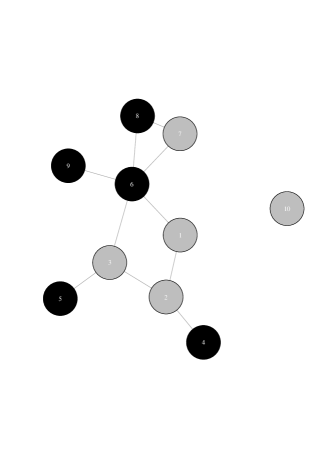
Figure 1: Undirected social network. (Note: Grey nodes are the control units and black nodes are treatment units)

Units	Observed Variables			Counterfactual Outcomes				Permuted Variables
$i$	$T_{i}$	$\Pi_{i}$	$Y^{obs}_{i}$	$Y_{i}(1,0)$	$Y_{i}(0,0)$	$Y_{i}(1,1)$	$Y_{i}(0,1)$	$\Lambda(T_{i})$	$\pi_{i}(\tilde{\mathbf{t}})$	$Y^{P}_{i}$
$1$	$0$	1	$y_{1}$	?	?	$y_{1}+\tau$	$y_{1}$	1	1	$y_{1}+\tau$
$2$	$0$	0	$y_{2}$	$y_{2}+\tau$	$y_{2}$	?	?	1	1	?
$3$	$0$	1	$y_{3}$	?	?	$y_{3}+\tau$	$y_{3}$	1	1	$y_{3}+\tau$
$4$	$1$	0	$y_{4}$	$y_{4}$	$y_{4}-\tau$	?	?	1	1	?
$5$	$1$	0	$y_{5}$	$y_{5}$	$y_{5}-\tau$	?	?	1	1	?
$6$	$1$	0	$y_{6}$	$y_{6}$	$y_{6}-\tau$	?	?	0	0	?
$7$	$0$	1	$y_{7}$	?	?	$y_{7}+\tau$	$y_{7}$	0	0	?
$8$	$1$	1	$y_{8}$	?	?	$y_{8}$	$y_{8}-\tau$	0	0	?
$9$	$1$	1	$y_{9}$	?	?	$y_{9}$	$y_{9}-\tau$	0	0	?
$10$	$0$	0	$y_{10}$	$y_{10}+\tau$	$y_{10}$	?	?	0	0	$y_{10}$

Table 1: A Science Table under $H_{0},$ using Example 3 .1. NB: $Y^{P}_{i}$ represents the new outcome of unit $i$ under $H_{0}$ for the new treatment vector $\tilde{\mathbf{t}}$.

To "sharpen" $H_{0}$ and obtain the null distributions of a test statistic $\mathrm{TS}_{k},$ for any $k,$ we propose a CRI method that applies the three-step conditioning procedure. First, to compute $\mathrm{TS}_{k},$ the relevant units are those with observed exposure value equal to $\pi_{k}.$ Hence, these units form the super focal units. Let $S_{k}$ be an indicator variable that marks the super focal status units, i.e.,

$$S_{ik}=\mathbbm{I}(\pi_{i}(\mathbf{t}^{obs})=\pi_{k})$$

Second, we let $\mathcal{T}_{k}$ represent the subset of treatment assignment vectors that imputes $\mathrm{TS}_{k},$ under the $H_{0},$ i.e.,

$$\mathcal{T}_{k}:=\{\mathbf{t}^{\prime}\in\{0,1\}^{N}:p(\mathbf{t}^{\prime})>0,\,\,R(0,\mathbf{t}^{\prime},\pi_{k})>\epsilon,\text{and}\,\,R(1,\mathbf{t}^{\prime},\pi_{k})>\epsilon\,\,\text{for some}\,\,\epsilon\in(0,0.5)\},$$ (18)

with,

$$R(t,\mathbf{t}^{\prime},\pi_{k})\coloneqq\frac{\sum_{i=1}^{N}\mathbbm{I}\{t^{\prime}_{i}=t,\pi_{i}(\mathbf{t}^{\prime})=\pi_{k},\pi_{i}(\mathbf{t}^{obs})=\pi_{k}\}}{\sum_{i=1}^{N}\mathbbm{I}\{\pi_{i}(\mathbf{t}^{obs})=\pi_{k}\}}=\frac{\sum_{i=1}^{N}\mathbbm{I}\{t^{\prime}_{i}=t,\pi_{i}(\mathbf{t}^{\prime})=\pi_{k},\pi_{i}(S_{ik}=1\}}{\sum_{i=1}^{N}\mathbbm{I}\{S_{ik}=1\}},$$ (19)

where, $R(\cdot,\cdot,\cdot)$ denotes the empirical probability or relative frequency. In words, $\mathcal{T}_{k}$ is the subset of treatment assignment vectors satisfying the treatment assignment mechanism $p,$ and ensures that a "sufficient" number of units with the different treatments $(t=0,1)$ have exposure values fixed at $\pi_{k}$. In (18), the tuning parameter $\epsilon$ controls the minimum number of units with an exposure value of $\pi_{k}$ under the permuted treatment vector.

By construction, the sets $\mathcal{T}_{k},\,\,\text{for}\,\,k=1,\dots K,$ depend on the sample size and the exposure mapping. For each $k$, the cardinality of $\mathcal{T}_{k}$ may be higher when the sample size is large. Also, exposure mappings with a smaller range of values (e.g., threshold functions of the treatment vectors of neighbors that produce binary exposure values as in Example 3 .1) are more likely to produce larger $\mathcal{T}_{k}$ sets. Note that the power and size distortions of the conditional randomization test depend on the cardinality of $\mathcal{T}_{k}.$

Third, we let $F_{k}(\mathbf{t}^{\prime})$ denote the indicator variable for the focal units we use to compute $\mathrm{TS}_{k}$ when the treatment assignment vector is $\mathbf{t}^{\prime}.$ Therefore, for unit $i$, we define

$$F_{ik}(\mathbf{t}^{\prime}):=\mathbbm{I}(\pi_{i}(\mathbf{t}^{\prime})=\pi_{k},\pi_{i}(\mathbf{t}^{obs})=\pi_{k})=\mathbbm{I}(\pi_{i}(\mathbf{t}^{\prime})=\pi_{k},S_{ik}=1),\,\,\,\forall\mathbf{t}^{\prime}\in\mathcal{T}_{k}.$$ (20)

In other words, the focal units (for a given treatment vector that belongs to the subset of treatment assignment vectors) are the units whose exposure values remain the same as the exposure values under the observed treatment assignment vector. Thus, they are units from the super-focal units set. By construction, for $\mathbf{t}^{\prime},\mathbf{t}^{\prime\prime}\in\mathcal{T}_{k},\,\,\text{where}\,\,\mathbf{t}^{\prime}\neq\mathbf{t}^{\prime\prime},$ it is possible that $F_{ik}(\mathbf{t}^{\prime})\neq F_{ik}(\mathbf{t}^{\prime\prime}),$ meaning unit $i$ may be a focal unit to impute $\mathrm{TS}_{k}(\mathbf{Y}^{obs},\mathbf{t}^{\prime},\mathbf{A})$ but a non-focal unit to impute $\mathrm{TS}_{k}(\mathbf{Y}^{obs},\mathbf{t}^{\prime\prime},\mathbf{A})$ and vice-versa. Hence, the number of focal units $\sum_{i=1}^{N}F_{ik}(\mathbf{t}^{\prime})$ is random across $\mathbf{t}^{\prime}\in\mathcal{T}_{k}$. In particular, for $\mathbf{t}^{\prime}\in\mathcal{T}_{k},$ the number of focal units is:

$$\sum_{i=1}^{N}F_{ik}(\mathbf{t}^{\prime})=N_{k}\cdot\sum_{t\in\{0,1\}}R(t,\mathbf{t}^{\prime},\pi_{k}).$$ (21)

This shows that we control the average number of focal units when choosing the subset of treatment assignment vectors $\mathcal{T}_{k}$ via the tuning parameter $\epsilon.$

Now using the definitions in (18) and (20), and a slight abuse of notation, the test statistics in (14) conditional on the subsets of focal units and treatment assignment vectors is

$$\mathrm{TS}_{k}(\mathbf{Y},\mathbf{T},\mathbf{A};\mathcal{T}_{k},F_{k})=\mathrm{TS}_{k}(\mathbf{Y},\mathbf{T},\mathbf{A}|\mathbf{T}\in\mathcal{T}_{k},F_{k}(\mathbf{T})=1)$$

Consequently, for each $\mathrm{TS}_{k},k=1,\dots,K,$ we can define the conditional p-value under $H_{0}$ as

$$pval_{{}_{k}}(\mathbf{T},\mathbf{Y}^{obs};\mathcal{T}_{k},F_{k},F_{k}^{obs}):=\mathbbm{E}_{\mathcal{T}_{k}}[\mathbbm{I}\{\mathrm{TS}_{k}(\mathbf{Y}_{F_{k}}(\mathbf{t}^{*}),\mathbf{t}^{*},\mathbf{A};\mathcal{T}_{k},F_{k})\geq\mathrm{TS}_{k}(\mathbf{Y}^{obs},\mathbf{t}^{obs},\mathbf{A};F^{obs}_{k})\}|\mathbf{t}^{*}\in\mathcal{T}_{k},H_{0}],$$ (22)

where $\mathbf{Y}_{F_{k}}(\mathbf{t}^{*})$ denotes the component vector of outcomes for the focal units when treatment assignment vector is $\mathbf{t}^{*}$ under $H_{0}.$ The expectation notation $\mathbbm{E}_{\mathcal{T}_{k}}$ is to emphasize that the probability is with respect to $\mathbf{t}^{*}\in\mathcal{T}_{k}.$ Also, note that the observed test statistic, $\mathrm{TS}_{k}(\mathbf{Y}^{obs},\mathbf{t}^{obs},\mathbf{A};F_{k}^{obs})$ in Definition (22) is conditional on a subset of super focal units with indicator variable $F_{k}^{obs}.$

Remark 1.

It is worth noting that $F_{k}^{obs}\neq F_{k},$ i.e., the indicator variable for focal units of the permuted treatment vectors is not the same as the indicator variable for the focal units we use to compute the observed test statistic. So, what is the definition of $F_{k}^{obs},$ or which individuals should be used in calculating the observed test statistic? Since the number of focal units is random across the permuted treatment vectors, we select a random subset of units from the super focal units to compute the observed test statistic. The size of the random subset of units to compute the observed test statistic must equal the expected number of focal units across permuted treatment vectors to guarantee the asymptotic validity of the testing procedures.

Next, we look at the conditioning procedure for the combined test statistic of $H_{0}.$ Formally, we write the combined test statistic as

$$\mathrm{TS}(\mathbf{Y},\mathbf{T},\mathbf{A}):=f(\mathrm{TS}_{1},\dots,\mathrm{TS}_{k},\dots,\mathrm{TS}_{K})=\sum_{k=1}^{K}\Pr(\Pi=\pi_{k})\cdot\mathrm{TS}_{k}.$$ (23)

It is also not imputable for all treatment assignment vectors. All experimental units are relevant in computing $\mathrm{TS}.$ Therefore, the super-focal units indicator variable denoted by $S$ is

$$S=\mathbbm{I}(\pi_{i}(\mathbf{t}^{obs})=\pi_{1}\vee\pi_{i}(\mathbf{t}^{obs})=\pi_{2}\vee\dots\vee\pi_{i}(\mathbf{t}^{obs})=\pi_{k}),$$

where $\vee$ is the $\mathrm{OR}$ notation.

Also, for the combined test statistic, the treatment assignment vectors that guarantee the "imputability" of the test statistic are those that ensure that there are "sufficient" units to compute all the individual $\mathrm{TS}_{k},$ for $k=1,\dots,K.$ It is a more stringent requirement compared to the conditions for the individual test statistics. This suggests that the conditioning events depend on the choice of the testing approach. Formally, we let $\mathcal{T}$ represent the subset of treatment assignment vectors that impute $\mathrm{TS},$ i.e.,

$$\mathcal{T}:= \{\mathbf{t}^{\prime}\in\{0,1\}^{N}:p(\mathbf{t}^{\prime})>0,R(1,\mathbf{t}^{\prime},\pi_{k})>\epsilon,\,\,\text{and}\,\,R(0,\mathbf{t}^{\prime},\pi_{k})>\epsilon,\,\,\forall k=1,\dots,K,\epsilon\in(0,0.5)\}$$

$$= \cap_{k=1}^{K}\mathcal{T}_{k}.$$ (24)

By construction, $|\mathcal{T}|\leq|\mathcal{T}_{k}|$ for all $k=1,\dots,K.$ Therefore, the sample size and the exposure mapping requirements for this test statistic may be more demanding.

Finally, as with the multiple-testing approach, the identity of focal units also depends on the treatment assignment vector. If we let $F(\mathbf{t}^{\prime})$ denote the indicator variable for the focal units that we use to compute the test statistic, $\mathrm{TS},$ when the treatment assignment vector is $\mathbf{t}^{\prime}$, then for each unit $i,$ we have

$$F_{i}(\mathbf{t}^{\prime}):= \mathbbm{I}(\pi_{i}(\mathbf{t}^{\prime})=\pi_{k},\pi_{i}(\mathbf{t^{obs}})=\pi_{k})=\mathbbm{I}(\pi_{i}(\mathbf{t}^{\prime})=\pi_{k},S=1)\,\,\,\forall k=1,\dots,K\,\,\,\forall\mathbf{t}^{\prime}\in\mathcal{T}.$$ (25)

From the construction of $F,$ the focal units are not fixed but vary with the treatment assignment vector. In particular, the number of focal units for $\mathbf{t}^{\prime}\in\mathcal{T}_{k}$ is

$$\sum_{i=1}^{N}F_{i}(\mathbf{t}^{\prime})=\sum_{k=1}^{K}\Bigg{(}N_{k}\sum_{t\in\{0,1\}}R(t,\mathbf{t}^{\prime},\pi_{k})\Bigg{)},$$ (26)

which also shows that we control the average number of focal units when choosing $\mathcal{T}$ via the tuning parameter.

Now, using (3 .2.1), (25), and a slight abuse of notation, we rewrite the conditional combined test statistics conditional on the focal units and $\mathcal{T}$ as

$$\mathrm{TS}(\mathbf{Y},\mathbf{T},\mathbf{A};\mathcal{T},F)=\mathrm{TS}(\mathbf{Y},\mathbf{T},\mathbf{A}|\mathbf{T}\in\mathcal{T},F(\mathbf{T})=1),$$

and the conditional p-value becomes

$$pval(\mathbf{T},\mathbf{Y}^{obs};\mathcal{T},F,F^{obs}):=\mathbbm{E}_{\mathcal{T}}[\mathbbm{I}\{\mathrm{TS}(\mathbf{Y}_{F}(\mathbf{t}^{*}),\mathbf{t}^{*},\mathbf{A};\mathcal{T},F)\geq\mathrm{TS}(\mathbf{Y}^{obs},\mathbf{t}^{obs},\mathbf{A};F^{obs})\}|\mathbf{t}^{*}\in\mathcal{T},H_{0}],$$ (27)

where $\mathbf{Y}_{F}(\mathbf{t}^{*})$ is the vector of outcomes for the focal units when the treatment assignment vector is $\mathbf{t}^{*}$ under the $H_{0}.$ The expectation notation $\mathbbm{E}_{\mathcal{T}}$ emphasizes that the probability is with respect $\mathbf{t}^{*}\in\mathcal{T}.$

Remark 2.

For the combined test statistic, too, note that $F^{obs}\neq F,$, i.e., the indicator variable for focal units of the permuted treatment vectors is not the same as the indicator variable for the focal units we use to compute the observed test statistic. We follow the recommendation in Remark 1 to select the focal units to calculate the observed test statistic.

The drawback of our proposed CRI method is that, with a small sample size, the subsample sizes $N_{k},k=1,\dots,K$ (which is the size of super focal units) may be very small. Therefore, selecting focal units less than $N_{k}$ may produce imprecise estimates of the test statistics that lead to erroneous p-values. Nevertheless, using the test statistics $\mathrm{TS}_{k}$ and $\mathrm{TS},$ we show the asymptotic validity of the proposed CRI method when the nuisance parameter $\tau$ is known. The following theorem states the asymptotic validity results for the proposed CRI method given $\tau$ and the test statistics for $H_{0}.$

Theorem 1 (Asymptotic validity of CRI method with known nuisance parameters).

Suppose Assumptions 1-4 hold, and the variation in outcomes is finite across the population. Also, let $0<\epsilon<0.5,$ and assume that the true value of $\tau$ is known.
i) Under the null hypothesis $H_{0}$ in (8), using the three-step conditional randomization testing procedure with the test statistic $\mathrm{TS}_{k}$ is asymptotically valid at any significant level $\alpha$,

$$\lim_{N\to\infty}\Pr(pval_{{}_{k}}(\mathbf{T},\mathbf{Y}^{obs};\mathcal{T}_{k},F_{k},F_{k}^{obs})\leq\alpha|H_{0})\leq\alpha\,\,\text{for any}\,\,\alpha\in[0,1],$$ (28)

where the observed test statistic is calculated using the recommendation in Remark 1.
ii) Under the null hypothesis $H_{0}$ in (8), the three-step conditional randomization testing procedure with the test statistic $\mathrm{TS}$ is valid at any level $\alpha,$

$$\lim_{N\to\infty}\Pr(pval(\mathbf{T},\mathbf{Y}^{obs};\mathcal{T},F,F^{obs})\leq\alpha|H_{0})\leq\alpha\,\,\text{for any}\,\,\alpha\in[0,1],$$ (29)

where the observed test statistic is calculated using the recommendation in Remark 2. In both inequalities, the probabilities are with respect to $p.$

It is worth noting that the asymptotic regime in this paper is the same as that employed in Sävje et al. (2021). In this regime (inspired by Isaki and Fuller (1982)), it is assumed that there is an arbitrary sequence of non-nested finite samples. The proof of Theorem 1(i) is relegated to Appendix Lemmas and Proofs. It is easy to demonstrate that any multiple testing procedure that employs the marginal p-values $pval_{{}_{k}},k=1,\dots,K,$ is asymptotically valid. Therefore, we omit the proof.

3 .2.2 $H_{0}^{\Pi}$: Constant treatment effect within exposure values

Let us revisit Example 3 .1. Under $H_{0}^{\Pi}$, we have the corresponding science table in Table 2.

Units Observed Variables Counterfactual Outcomes Permuted Variables $i$ $T_{i}$ $\Pi_{i}$ $Y^{obs}_{i}$ $Y_{i}(1,0)$ $Y_{i}(0,0)$ $Y_{i}(1,1)$ $Y_{i}(0,1)$ $\Lambda(T_{i})$ $\pi_{i}(\tilde{\mathbf{t}})$ $Y^{P}_{i}$ $1$ $0$ 1 $y_{1}$ ? ? $y_{1}+\tau(1)$ $y_{1}$ 1 1 $y_{1}+\tau(1)$ $2$ $0$ 0 $y_{2}$ $y_{2}+\tau(0)$ $y_{2}$ ? ? 1 1 ? $3$ $0$ 1 $y_{3}$ ? ? $y_{3}+\tau(1)$ $y_{3}$ 1 1 $y_{3}+\tau(1)$ $4$ $1$ 0 $y_{4}$ $y_{4}$ $y_{4}-\tau$(0) ? ? 1 1 ? $5$ $1$ 0 $y_{5}$ $y_{5}$ $y_{5}-\tau(0)$ ? ? 1 1 ? $6$ $1$ 0 $y_{6}$ $y_{6}$ $y_{6}-\tau(0)$ ? ? 0 0 ? $7$ $0$ 1 $y_{7}$ ? ? $y_{7}+\tau(1)$ $y_{7}$ 0 0 ? $8$ $1$ 1 $y_{8}$ ? ? $y_{8}$ $y_{8}-\tau(1)$ 0 0 ? $9$ $1$ 1 $y_{9}$ ? ? $y_{9}$ $y_{9}-\tau(1)$ 0 0 ? $10$ $0$ 0 $y_{10}$ $y_{10}+\tau(0)$ $y_{10}$ ? ? 0 0 $y_{10}$

Table 2: A Science Table under $H^{\Pi}_{0},$ using Example 3 .1. NB: $Y^{P}_{i}$ represents the new outcome of unit $i$ under $H^{\Pi}_{0}$ for the new treatment vector $\tilde{\mathbf{t}}$.

Tables 1 and 2 are nearly identical. However, Table 2 has two nuisance parameters, $\tau(0)$ and $\tau(1)$, which correspond to two different exposure values for the network mapping in this example. Thus, in general, we require $K$ nuisance parameters to test $H_{0}^{\Pi}.$ If one knows these nuisance parameters, then the same principles for choosing the subset of treatment assignments and units, as well as the proposed test statistics for $H_{0},$ are applicable in testing for $H_{0}^{\Pi}$ as well.

3 .2.3 $H_{0}^{X,\Pi}$: Constant treatment effect across pretreatment variables and exposure values

Like $H_{0}$, the test statistic $\mathrm{TS}_{k,l}$ cannot be imputed due to similar reasons. Example 3 .2 expands on Example 3 .1 and illustrates the reason why $H_{0}^{X,\Pi}$ is not sharp.

Example 3 .2.

Assume there are $N=10$ units in an undirected social network, as in Figure 2. Our data is $(Y_{i},T_{i},\Pi_{i},X_{i})_{i=1}^{N},$ where $\Pi_{i}$ is defined in Example 3 .1. Table 3 shows that each unit has two missing potential outcomes. Hence, $H_{0}^{X,\Pi}$ is also not sharp. Now, using the permuted treatment vector $\tilde{\mathbf{t}}=(1,1,1,1,1,0,0,0,0,0),$ we can deduce that none of the test statistics $\mathrm{TS}_{kl},k=1,\dots,K\,\,\text{and}\,\,l=1,\dots,L$ is imputable under $H_{0}^{X,\Pi}.$ In other words, for each $\pi\in\{0,1\}$, and $x\in\{f,m\}$ there exist $\Lambda(\mathbf{T})=\mathbf{t}^{\prime}\in\{0,1\}^{N}$ where $p(\mathbf{t}^{\prime})>0,$ but $\sum_{i=1}^{N}\mathbbm{I}(\Lambda(T_{i})=t,\pi_{i}(\mathbf{t}^{\prime})=\pi,X_{i}=x)=0$ for either $t=0$ or $t=1.$

Units Observed Variables Counterfactual Outcomes Permuted Variables $i$ $T_{i}$ $\Pi_{i}$ $X_{i}$ $Y^{obs}_{i}$ $Y_{i}(1,0)$ $Y_{i}(0,0)$ $Y_{i}(1,1)$ $Y_{i}(0,1)$ $\Lambda(T_{i})$ $\pi_{i}(\tilde{\mathbf{t}})$ $Y^{P}_{i}$ $1$ $0$ 1 $m$ $y_{1}$ ? ? $y_{1}+\tau(1;m)$ $y_{1}$ 1 1 $y_{1}+\tau(1;m)$ $2$ $0$ 0 $m$ $y_{2}$ $y_{2}+\tau(0;m)$ $y_{2}$ ? ? 1 1 ? $3$ $0$ 1 $m$ $y_{3}$ ? ? $y_{3}+\tau(1;m)$ $y_{3}$ 1 1 $y_{3}+\tau(1;m)$ $4$ $1$ 0 $f$ $y_{4}$ $y_{4}$ $y_{4}-\tau(0;f)$ ? ? 1 1 ? $5$ $1$ 0 $f$ $y_{5}$ $y_{5}$ $y_{5}-\tau(0;f)$ ? ? 1 1 ? $6$ $1$ 0 $m$ $y_{6}$ $y_{6}$ $y_{6}-\tau(0;m)$ ? ? 0 0 ? $7$ $0$ 1 $f$ $y_{7}$ ? ? $y_{7}+\tau(1;f)$ $y_{7}$ 0 0 ? $8$ $1$ 1 $m$ $y_{8}$ ? ? $y_{8}$ $y_{8}-\tau(1;m)$ 0 0 ? $9$ $1$ 1 $f$ $y_{9}$ ? ? $y_{9}$ $y_{9}-\tau(1;f)$ 0 0 ? $10$ $0$ 0 $f$ $y_{10}$ $y_{10}+\tau(0;f)$ $y_{10}$ ? ? 0 0 $y_{10}$

Table 3: A Science Table under $H_{0}^{X,\Pi},$ using Example 3 .1. NB: $Y^{P}_{i}$ represents the new outcome of unit $i$ under $H_{0}^{X,\Pi}$ for the new treatment vector $\tilde{\mathbf{t}}$.

Figure 2: Undirected social network. (Note: Grey nodes are the control units and black nodes are treatment units. Circle nodes are females and square nodes are males.)

To generate the null distributions of any of the test statistics $\mathrm{TS}_{k,l},$ where the $L\times K$ nuisance parameters in $H_{0}^{X,\Pi}$ are known, we apply the three-step conditioning procedure. First, the relevant units to compute a given $\mathrm{TS}_{k,l},$ are those with exposure value of $\pi_{k}$ and pretreatment value $x_{l}.$ Thus, the indicator variable for the super-focal units denoted as $S_{kl}$ is

$$S_{ikl}=\mathbbm{I}(\pi_{i}(\mathbf{t}^{obs})=\pi_{k},X_{i}=x_{l})$$

Secondly, let $\mathcal{T}_{k,l}$ denote the subset of treatment assignment vectors that impute $\mathrm{TS}_{k,l}.$ Then,

$$\mathcal{T}_{k,l}:=\{\mathbf{t}^{\prime}\in\{0,1\}^{N}:p(\mathbf{t}^{\prime})>0,R(1,\mathbf{t}^{\prime},\pi_{k},x_{l})>\epsilon,\,\,\text{and}\,\,R(0,\mathbf{t}^{\prime},\pi_{k},x_{l})>\epsilon\,\,t=0,1,\epsilon\in(0,0.5)\},$$ (30)

with

$$R(t,\mathbf{t}^{\prime},\pi_{k},x_{l})\coloneqq\frac{\sum_{i=1}^{N}\mathbbm{I}\{t^{\prime}_{i}=t,\pi_{i}(\mathbf{t}^{\prime})=\pi_{k},\pi_{i}(\mathbf{t}^{obs})=\pi_{k},X_{i}=x_{l}\}}{\sum_{i=1}^{N}\mathbbm{I}\{\pi_{i}(\mathbf{t}^{obs})=\pi_{k},X_{i}=x_{l}\}}=\frac{\sum_{i=1}^{N}\mathbbm{I}\{t^{\prime}_{i}=t,\pi_{i}(\mathbf{t}^{\prime})=\pi_{k},S_{ikl}=1\}}{\sum_{i=1}^{N}\mathbbm{I}\{S_{ikl}=1\}},$$ (31)

where the $R(\cdot,\cdot,\cdot,\cdot)$ is an empirical probability. The set $\mathcal{T}_{k,l}$ is the subset of treatment assignment vectors (that respect the assignment mechanism) where there is a "sufficient" number of units in each of the arms of treatment and for a given pretreatment variable value $x_{l}$ that the exposure value remains fixed at $\pi_{k}.$

By construction, the sets $\mathcal{T}_{k,l},\,\,k=1,\dots,K\,\,\text{and}\,\,l=1,\dots,L$ depend on the sample size, the number of subgroups, and the number of exposure values. For each $k$ and $l$, the cardinality of $\mathcal{T}_{k,l}$ is bigger when we have a large sample and the number of covariate-defined subgroups is small. Also, exposure mappings with a smaller range of values are more likely to lead to a larger $|\mathcal{T}_{k,l}|.$

Lastly, we let $F_{k,l}(\mathbf{t}^{\prime})$ represent the indicator variable for the focal units when the treatment assignment vector is $\mathbf{t}^{\prime}.$ Therefore, for unit $i$, we have

$$F_{ik,l}(\mathbf{t}^{\prime}):=\mathbbm{I}(\pi_{i}(\mathbf{t}^{\prime})=\pi_{k},\pi_{i}(\mathbf{t}^{obs})=\pi_{k},X_{i}=x_{l})\,\,\,\forall\mathbf{t}^{\prime}\in\mathcal{T}_{k,l}.$$ (32)

Hence, for $\mathbf{t}^{\prime}\in\mathcal{T}_{k,l},$ the number of focal units is

$$\sum_{i=1}^{N}F_{ik,l}(\mathbf{t}^{\prime})=N_{k,l}\cdot\sum_{t\in\{0,1\}}R(t,\mathbf{t}^{\prime},\pi_{k},x_{l}),$$ (33)

where $N_{k,l}$ represents the number of units with $X=x_{l}$ and has observed exposure value of $\pi_{k}.$ Equation (33) indicates that we control the expected number of focal units using the tuning parameter $\epsilon$. In addition, when we compare (21) and (33), it is evident that the average number of focal units is smaller under the null $H_{0}^{X,\Pi}$ for each of the multiple test statistics. It suggests that one may require more data to test $H_{0}^{X,\Pi}$ compared to $H_{0}$ and $H_{0}^{\Pi}.$

Now, using the definitions in (30) and (32), and slightly abusing notation, the conditional test statistics can be written technically as

$$\mathrm{TS}_{k,l}(\mathbf{Y},\mathbf{T},\mathbf{A},\mathbf{X};\mathcal{T}_{k,l},F_{k,l})=\mathrm{TS}(\mathbf{Y},\mathbf{T},\mathbf{A}|\mathbf{T}\in\mathcal{T}_{k,l},F_{k,l}(\mathbf{T})=1,\mathbf{X}=x_{l}).$$

Therefore, for each $\mathrm{TS}_{k,l},$ we can also define the conditional p-value as

$$pval_{{}_{kl}}(\mathbf{T},\mathbf{Y}^{obs},\mathbf{X};\mathcal{T}_{k,l},F_{k,l},F^{obs}_{k,l}):=\mathbbm{E}_{\mathcal{T}_{k,l}}[\mathbbm{I}\{\mathrm{TS}_{k,l}(\mathbf{Y}_{F_{{}_{k,l}}}(\mathbf{t}^{*}),\mathbf{t}^{*},\mathbf{A},\mathbf{X};\mathcal{T}_{k,l},F_{k,l})\geq\mathrm{TS}_{k,l}(\mathbf{Y}^{obs},\mathbf{t}^{obs},\mathbf{A},\mathbf{X};F^{obs}_{k,l})\}|\mathbf{t}^{*}\in\mathcal{T}_{k,l},H_{0}^{X,\Pi}],$$ (34)

where $\mathbf{Y}_{F_{{}_{k,l}}}(\mathbf{t}^{*})$ is the vector of outcomes for focal units when treatment assignment vector is $\mathbf{t}^{*}.$ The expectation notation $\mathbbm{E}_{\mathcal{T}_{k,l}}$ emphasizes that the probability is with respect to $\mathbf{t}^{*}\in\mathcal{T}_{k,l}.$ To achieve asymptotic validity, $F^{obs}_{k,l}$ is also analogous to $F^{obs}_{k}.$

Shifting attention to the single testing approach for $H_{0}^{X,\Pi},$ we write the combined test statistic as the weighted sum of the $L\times K$ test statistics, i.e.,

$$\mathrm{TS}^{X,\Pi}(\mathbf{Y},\mathbf{T},\mathbf{A},\mathbf{X}):=f(\mathrm{TS}_{k,l}:x_{l}\in\mathbbm{X},k=1,\dots,K)=\sum_{k=1}^{K}\sum_{l=1}^{L}\Pr(\Pi=\pi_{k},X=x_{l})\cdot\mathrm{TS}_{k,l}.$$ (35)

This test statistic is also not imputable under $H_{0}^{X,\Pi}$. All experimental units are used to compute the test statistic; hence, the super-focal units indicator is $S.$

The treatment assignment vectors that guarantee the imputability of $\mathrm{TS}^{X,\Pi}$ are those that ensure that there are a "sufficient" number of units to compute all $\mathrm{TS}_{k,l}^{\prime}s.$ Let $\mathcal{T}^{X,\Pi}$ represent the subset of treatment assignment vectors that impute $\mathrm{TS}^{X,\Pi}.$ Then,

$$\mathcal{T}^{X,\Pi}:= \{\mathbf{t}^{\prime}\in\{0,1\}^{N}:p(\mathbf{t}^{\prime})>0,R(1,\mathbf{t}^{\prime},\pi_{k},x_{l})>\epsilon\,\,\text{and}\,\,R(0,\mathbf{t}^{\prime},\pi_{k},x_{l})>\epsilon,$$

$$\forall k=1,\dots,K\,\,\,\,\forall l=1,\dots,L\,\,\text{and}\,\,\epsilon\in(0,0.5)\,\,\}$$

$$= \cap_{k=1}^{K}\mathcal{T}_{k,l}$$ (36)

Note that, $|\mathcal{T}^{X,\Pi}|\leq|\mathcal{T}_{k,l}|$ for all $k=1,\dots,K,$ and $l=1,\dots,L.$ Therefore, the combined test statistic’s sample size and exposure mapping requirements may be more tasking than those for each $\mathrm{TS}_{kl}.$

The definition of the focal units is the same as the one for the combined test statistics of $H_{0}$ in (25). This is because pretreatment variables are not causal but control variables.

With a slight abuse of notation, the combined test statistics $\mathrm{TS}^{X,\Pi}$ conditional on the subset of treatment assignment vectors and the focal units can also be written as

$$\mathrm{TS}^{X,\Pi}(\mathbf{Y},\mathbf{T},\mathbf{X},\mathbf{A};\mathcal{T}^{X,\Pi},F)=\mathrm{TS}(\mathbf{Y},\mathbf{T},\mathbf{X},\mathbf{A}|\mathbf{T}\in\mathcal{T}^{X,\Pi},F(\mathbf{T})=1)$$

and the resulting conditional p-value is

$$pval(\mathbf{T},\mathbf{Y}^{obs},\mathbf{X};\mathcal{T}^{X,\Pi},F,F^{obs}):=\mathbbm{E}_{\mathcal{T}^{X,\Pi}}[\mathbbm{I}\{\mathrm{TS}(\mathbf{Y}_{F}(\mathbf{t}^{*}),\mathbf{t}^{*},\mathbf{X},\mathbf{A};\mathcal{T}^{X,\Pi},F)\geq\mathrm{TS}(\mathbf{Y}^{obs},\mathbf{T},\mathbf{X},\mathbf{A};F^{obs})\}|\mathbf{t}^{*}\in\mathcal{T}_{k,l},H_{0}^{X,\Pi}],$$ (37)

where the expectation notation $\mathbbm{E}_{\mathcal{T}^{X,\Pi}}$ emphasizes that the probability is with respect to $\mathbf{t}^{*}\in\mathcal{T}^{X,\Pi}.$

In practice, the sets $\mathcal{T}_{k},$ $\mathcal{T},$ $\mathcal{T}_{k,l}$ and $\mathcal{T}^{X,\Pi}$ may be large and one may have to approximate the p-values in (22), (27), (34), and (37). We recommend drawing a random sample of elements of size $B$ from these sets to compute the p-values. The following algorithm summarizes our proposed CRI testing procedure with known nuisance parameters.

Data: $(\mathbf{Y}^{obs},\mathbf{T},\mathbf{A},\mathbf{X},\{\Pi_{i}\}_{i}^{N})$

Result: the estimated p-values: e.g., $\widehat{pval}_{k}(\mathbf{T},\mathbf{Y}^{obs};\mathcal{T}_{k},F_{k},F^{obs}_{k})$

1. Compute the test statistic using the appropriate random subset of super focal units from the observed data: e.g., $\mathrm{TS}_{k}(\mathbf{Y}^{obs},\mathbf{t}^{obs},\mathbf{A};F^{obs}).$

2. Choose $\epsilon.$

3. for {$b=1$ to $B$} do

       Draw $\mathbf{t}^{(b)}$ independently from the appropriate subset of treatment assignment vectors , e.g.,$\mathcal{T}_{k}.$

       Compute the test statistic using $\mathbf{t}^{(b)}$ and the focal units, e.g., $\mathrm{TS}_{k}(\mathbf{Y}^{obs},\mathbf{t}^{(b)},\mathbf{A};\mathcal{T}_{k},F_{k})$

      

end for

4. Compute the empirical p-value, e.g.,

        $\widehat{pval}_{k}(\mathbf{T},\mathbf{Y}^{obs};\mathcal{T}_{k},F_{k},F^{obs}_{k})=B^{-1}\sum_{b=1}^{B}\mathbbm{I}\{\mathrm{TS}_{k}(\mathbf{Y}_{F_{{}_{k}}}(\mathbf{t}^{(b)}),\mathbf{t}^{(b)},\mathbf{A};\mathcal{T}_{k},F_{k})\geq$    

                                                                                                              $\mathrm{TS}_{k}(\mathbf{Y}^{obs},\mathbf{t}^{obs},\mathbf{A};F_{k}^{obs})\}$

Algorithm 1 Conditional Randomization Test Algorithm for HTE with known nuisance parameters

Under the null hypotheses, we can show that the procedures using the empirical p-values are also asymptotically valid. For instance, we can show that $\lim_{N\to\infty}\Pr(\widehat{pval}_{k}(\mathbf{T},\mathbf{Y}^{obs};\mathcal{T}_{k},F_{k},F^{obs}_{k})\leq\alpha)\leq\alpha\,\,\text{for any}\,\,\alpha\in[0,1],$ where the probability reflects variations in both treatment assignment and the sampling of treatment vectors from $\mathcal{T}_{k}.$ In fact, this validity results hold for any $B.$ However, the larger the value of $B$, the less the approximation error, $\widehat{pval}_{k}-pval.$ Finally, note that we can easily extend Theorem 1 to $H_{0}^{\Pi}$ and $H_{0}^{X,\Pi}.$

Since our proposed condition method depends on the tuning parameter $\epsilon,$ it is worthwhile to comment on it.

Remark 3.

The CRI method’s statistical power and computation time are affected by the tuning parameter, $\epsilon.$ Setting $\epsilon$ to a value closer to 0.5 decreases the subset of treatment assignment vectors’ cardinality, making the testing process computationally expensive and conservative. However, values of $\epsilon$ closer to 0.5 guarantees a large number of focal units for each treatment vector.

Therefore, the precision of the p-value depends on $\epsilon$ through two channels. Firstly, it affects the number of focal units, which directly affects the test statistics’ precision and, hence, the p-value’s precision. Secondly, $\epsilon$ affects the size of the subset of treatment assignment vectors, which directly affects the precision of the estimated p-value. As a result, a trade-off exists, and it is advisable to choose $\epsilon$ values between 0 and the minimum of the probabilities $\Pr(T=t,\Pi=\pi_{k})$ for all $t=0,1$ and $k=1,\dots,K$ for the null hypotheses $H_{0}$ and $H_{0}^{\Pi}.$

For instance, suppose the sample is balanced in terms of the treatment assignment variable and a binary exposure variable. In that case, choosing values of $\epsilon$ that lie in the middle of the $(0,0.5)$ range is recommended. We can apply the same choice strategy to all other null hypotheses.

3 .2.4 Comparison with existing conditioning procedures

The conditioning procedure we propose in this paper is most closely related to that in Basse et al. (2019). The authors provide a formal concept of a conditioning mechanism that helps to construct valid conditional randomization tests under interference. They build on the conditioning procedure in Athey et al. (2018) that explicitly advised against conditioning mechanisms that use treatment assignment or functions of treatment assignment. Basse et al. (2019) show that using treatment assignment as a conditioning variable is appropriate since it may improve statistical power.

The idea in Basse et al. (2019) is to set a conditioning event space based on units and treatment assignment vectors $\mathbbm{C}=\{(\mathcal{U},\mathcal{T}):\mathcal{U}\subseteq\mathbbm{U},\mathcal{T}\subseteq\{0,1\}^{N}\},$ where $\mathbbm{U}$ denotes the power set of units. And then draw a conditioning event $\mathcal{C}=(\mathcal{U},\mathcal{T})$ from $\mathbbm{C}$ with probability $m(\mathcal{C}|\mathbf{T})$ such that, conditional on $\mathcal{C},$ a test statistic $z(\mathbf{Y}^{obs},\mathbf{T},\mathbf{X},\mathbf{A},\mathcal{C})$ is imputable with respect to the null hypothesis. They refer to the probability $m(\mathcal{C}|\mathbf{T})$ as the conditioning mechanism, which together with the treatment assignment mechanism $p$ induces joint distribution $\Pr(\mathbf{T},\mathcal{C})=m(\mathcal{C}|\mathbf{T})\cdot p(\mathbf{T}).$ The mathematical simplification of the conditioning mechanism is

$$m(\mathcal{C}|\mathbf{T})=f(\mathcal{U}|\mathbf{T})\cdot g(\mathcal{T}|\mathcal{U},\mathbf{T}),$$ (38)

where $f$ and $g$ are distributions over $\mathbbm{U}$ and $\{0,1\}^{N}$ respectively. In other words, (38) suggests a two-step conditioning procedure where focal units are chosen based on treatment assignment, and then the subset of treatment assignment vectors are selected based on the focal units and treatment assignment.

In contrast, our conditioning procedure described in Section 3 .2, draws a conditioning event $\mathcal{C}^{\prime}=(\mathcal{S},\mathcal{U},\mathcal{T})$ from $\{(\mathcal{S},\mathcal{U},\mathcal{T}):\mathcal{S}\subseteq\mathbbm{U},\mathcal{U}\subseteq\mathcal{S},\mathcal{T}\subseteq\{0,1\}^{N}\}$ with probability $m^{\prime}(\mathcal{C}^{\prime}|\mathbf{T})$ such that, conditional on $\mathcal{C}^{\prime},$ a test statistic $z(\mathbf{Y}^{obs},\mathbf{T},\mathbf{X},\mathbf{A},\mathcal{C}^{\prime})$ is imputable with respect to the null hypothesis. Here, $\mathcal{S}$ denotes the super focal units, and $\mathcal{U}$ denotes the focal units. Our conditioning mechanism and the treatment assignment mechanism $p$ also induce joint distribution $\Pr(\mathbf{T},\mathcal{C}^{\prime})=m^{\prime}(\mathcal{C}^{\prime}|\mathbf{T})\cdot p(\mathbf{T}).$ Our conditioning mechanism simplifies as

$$m^{\prime}(\mathcal{C}^{\prime}|\mathbf{T})=f(\mathcal{S}|\mathbf{T})\cdot g(\mathcal{T}|\mathcal{S},\mathbf{T})\cdot f(\mathcal{U}|\mathcal{S},\mathbf{T},\mathcal{T})$$ (39)

Equation (39) summarizes our three-step conditioning procedure, where super focal units are chosen based on treatment assignment. The subset of treatment assignment vectors is selected based on the super focal units and treatment assignment. The last step involves selecting the focal units based on treatment assignment, super focal units, and the subset of treatment assignment vectors. Comparing, (38) to (39) shows that the conditioning procedure in this paper generalizes that described in Basse et al. (2019). We highlight two key differences.

First, the choice of the subset of treatment assignments vectors and the focal units are interrelated via the super focal units. Specifically, our proposed procedure chooses the subset of treatment assignment vectors to maximize the number of focal units. It selects the set of focal units to optimize the cardinality of the subset of treatment assignment vectors. In contrast, the approach of Basse et al. (2019) suggests a prior random or non-random selection of focal units that depends on treatment assignment but not on the subset of treatment assignment vectors. Our procedure guarantees a larger subset of treatment assignment vectors, leading to higher statistical power and lower size distortion in general.

Second, our conditioning procedure allows focal units to vary across the elements in the subset of treatment assignment vectors. Simply put, the number of focal units can differ based on the treatment assignment vector, which sets it apart from previous methods. Specifically, the number of focal units is a binomial random variable (across the subset of treatment assignment vectors), which depends on the tuning parameter $\epsilon.$ Although allowing the focal units to vary across treatment assignments may lead to invalid p-values in small samples, it increases the cardinality of the subset of treatment assignment vectors, improving asymptotic statistical power and size. For example, suppose we have a population of four units, with two of them treated and paired into two dyads. Then, testing the null hypothesis of no spillovers, the approaches of Athey et al. (2018) and Basse et al. (2019) produce a subset of treatment assignment vectors of size two. However, allowing focal units to vary across treatment assignments leads to a subset of treatment assignment vectors of size four. Depending on the test statistic, all four treatment assignments may be useful in approximating the null distribution of the test statistic, leading to improvement in statistical power and size.

To sum, our proposed CRI method is a methodological contribution of the current paper. It offers fresh perspectives on choosing focal units and the subset of treatment assignment vectors. It is a generalization of the existing approaches and allows randomization tests of non sharp nulls using experimental data and observational data in the local randomization based regression discontinuity design setting. For instance, if we set $R(t,\mathbf{t}^{\prime},\pi_{k})$ in (18) such that $R(0,\mathbf{t}^{\prime},\pi_{k})+R(1,\mathbf{t}^{\prime},\pi_{k})=1$ for all $\mathbf{t}^{\prime}\in\mathcal{T}_{k},$ then $\mathcal{T}_{k}$ will coincide with the subset of treatment assignment vectors one would obtain using the existing approaches. In such a scenario, the focal units become fixed and uniformly larger (across the subset of treatment assignment vectors). However, it is computationally expensive and lowers the cardinality of the subset of treatment assignment vectors, resulting in low statistical power and high size distortions.

3 .3 Dealing with Unknown Nuisance Parameters

To implement our proposed CRI method, knowledge of the nuisance parameters is necessary. Unfortunately, these parameters are often unknown in practical applications. A natural but naive approach is to replace the unknown nuisance parameters with their sample counterparts and then apply the CRI method. Unfortunately, this testing procedure is invalid, both in finite samples and asymptotically. To understand why this approach is flawed, looking at the definition of randomization hypothesis (Lehmann and Romano, 2022, p. 832) is helpful.

Definition 3 .1 (Randomization Hypothesis).

Under the null hypothesis $H_{0}^{G}$, the distribution of the original sample data $(\mathbf{Y}^{obs},\mathbf{T},\Pi,\mathbf{X})$ is the same as the distribution of the samples we generate by replacing $\mathbf{T}$ with a new treatment vector $\Lambda(\mathbf{T})$ that respects the treatment assignment mechanism.

Definition 3 .1 is the crucial condition that guarantees the validity of randomization-based inferential methods. The practical consequence of this definition is that, under the null hypotheses, the distribution of the test statistic generated using the original data is the same as the distributions of the test statistic we obtain using data we generate with a new treatment vector that respects the treatment assignment mechanism.

Unfortunately, estimated nuisance parameters lead to a breakdown of the randomization hypothesis, and we illustrate it using the following example.

Example 3 .3.

Suppose our sample comprises four $(N=4)$ individuals with the original sample data given as $(\mathbf{Y}^{obs}=\{y_{1},y_{2},y_{3},y_{4}\},\mathbf{T}=\{1,1,0,0\},\Pi=\{\pi_{1},\pi_{1},\pi_{1},\pi_{1}\}).$ Consider the null hypothesis $H_{0}$ and estimate the nuisance parameter $\tau$ using the difference in means estimator, i.e., $\hat{\tau}=(y_{1}+y_{2}-y_{3}-y_{4})/2.$ Now, substituting $\hat{\tau}$ for $\tau$ into the null hypothesis in (8), we can impute all missing potential outcomes. If we choose a new treatment vector $\Lambda(\mathbf{T})=\mathbf{t}^{{}^{\prime\prime}}=\{0,0,1,1\}$ and assume that the exposure values remain the same under $\mathbf{t}^{{}^{\prime\prime}},$ then our new sample data is $(\mathbf{Y}^{{}^{\prime\prime}}=\{(y_{1}-y_{2}+y_{3}+y_{4})/2,(y_{2}-y_{1}+y_{3}+y_{4})/2,(y_{1}+y_{2}+y_{3}-y_{4})/2,(y_{1}+y_{2}-y_{3}+y_{4})/2\},\Lambda(\mathbf{T})=\{0,0,1,1\},\Pi^{\prime\prime}=\{\pi_{1},\pi_{1},\pi_{1},\pi_{1}\}).$ When we compare $\mathbf{Y}^{obs}$ to $\mathbf{Y}^{{}^{\prime\prime}},$ it is clear that under $H_{0},$ the distributions of the original sample and the new sample are not the same. Specifically, the new sample’s dependency structure differs from the original sample’s. Therefore, the distribution of test statistics that inherit the underlying distributional properties of the two samples will also be different even if $H_{0}$ is true.

Example 3 .3 highlights a challenge in replacing nuisance parameters with their sample counterparts in hypotheses. The example demonstrates that substituting estimated nuisance parameters in randomization tests can lead to a higher likelihood of rejecting accurate null hypotheses due to a breakdown in the randomization hypothesis. This issue persists not only in finite samples but also asymptotically.

To overcome this challenge, we offer two approaches: the sample splitting technique and the confidence interval technique. These methods can effectively handle unknown nuisance parameters.

3 .3.1 Sample Splitting Technique

The technique of sample splitting (SS) resolves the issue of estimated nuisance parameters by randomly dividing the original data into two equally balanced sub-samples. To the best of our knowledge, this is the first paper to apply a sample splitting approach to resolve the issue of nuisance parameters in randomization tests. When combined with our proposed conditioning approach (CRI method), we show below that the resulting procedure is asymptotically valid. The proposed SS technique involves three steps:

1. Randomly split the full sample into two equal and balanced sub-samples $\mathcal{U}^{est}$ and $\mathcal{U}^{inf}$. We use $\mathcal{U}^{est}$ for the estimation of the nuisance parameters and $\mathcal{U}^{inf}$ to test the hypothesis. Hence, $\mathcal{U}^{est}$ and $\mathcal{U}^{inf}$ denote the estimation and inference sub-samples respectively.

2. Estimate the nuisance parameter(s) using $\mathcal{U}^{est}$.

3. Permute the full treatment vector while respecting the treatment assignment mechanism, recalculate the exposure values for the full sample, and compute the test statistics using $\mathcal{U}^{inf}.$

Due to network interference, it is critical to permute the full treatment vector rather than the treatment vector of the inference sub-sample. This ensures that the full sample’s network structure is taken into account in the recalculation of the exposure values. It is the notable difference between our sample splitting method and other splitting schemes for different purposes in the econometrics, statistics, and machine learning literature. Alternatively, if the network is clustered, then the sample can be split into two with one set of clusters serving as the estimation subsample and the other set as the inference subsample.

Let us revisit Example 3 .3 to understand why the proposed technique works. Earlier, we established that the randomization hypothesis fails in this example when we replace the nuisance parameter with its sample counterpart.

Now, let us apply the SS technique. A possible balanced split of the original sample data into two is $\mathcal{U}^{est}=(\mathbf{Y}_{est}^{obs}=\{y_{1},y_{3}\},\mathbf{T}_{est}=\{1,0\},\Pi_{est}=\{\pi_{1},\pi_{1}\})$ and $\mathcal{U}^{inf}=(\mathbf{Y}^{obs}_{inf}=\{y_{2},y_{4}\},\mathbf{T}_{inf}=\{0,1\},\Pi_{inf}=\{\pi_{1},\pi_{1}\}).$ We compute the difference in means estimator of $\tau$ using $\mathcal{U}^{est},$ i.e., $\hat{\tau}^{est}=y_{1}-y_{3}.$ Under $H_{0},$ a new treatment vector $\Lambda(\mathbf{T})=\mathbf{t}^{{}^{\prime\prime}}=\{0,0,1,1\}$ produces a new inference sub-sample $\mathcal{U}^{inf}_{{}^{\prime\prime}}=(\mathbf{Y}^{{}^{\prime\prime}}_{inf}=\{y_{2}-\hat{\tau}^{est},y_{4}+\hat{\tau}^{est}\},\mathbf{t}^{{}^{\prime\prime}}_{inf}=\{0,1\},\Pi^{\prime\prime}_{inf}=\{\pi_{1},\pi_{1}\})=(\mathbf{Y}^{{}^{\prime\prime}}_{inf}=\{(y_{2}-y_{1}+y_{3}),(y_{4}+y_{1}-y_{3})\},\mathbf{t}^{{}^{\prime\prime}}_{inf}=\{0,1\},\Pi^{\prime\prime}_{inf}=\{\pi_{1},\pi_{1}\}).$

When the sample size is sufficiently large such that the difference between the estimated treatment effect and the true treatment effect is negligible, the distributions of the test statistic become equivalent when conditioned on either $\mathcal{U}^{inf}$ or $\mathcal{U}^{inf}_{{}^{\prime\prime}}$. This is due to the non-stochastic nature of $\hat{\tau}^{est}$ in the inference sub-sample $\mathcal{U}^{inf}_{{}^{\prime\prime}}$. Consequently, the randomization hypothesis, which does not hold in the case of using the complete sample data for estimation and inference, is valid when we employ the sample-splitting technique.

Under the null hypothesis $H_{0},$ and for the test statistic $\mathrm{TS}_{k}(\mathbf{Y},\mathbf{T},\mathbf{A};\mathcal{T}_{k},F_{k})$, we denote the p-value using the SS technique on the CRI method as $pval_{{}_{k}}(\mathbf{T},\mathbf{Y}^{obs};\mathcal{T}_{k},F_{k},F^{obs}_{k},\hat{\tau}^{est}).$ Similarly, for the combined test statistic $\mathrm{TS}(\mathbf{Y}^{obs},\mathbf{T},\mathbf{A};\mathcal{T},F)$, we denote the p-values we obtain from applying the SS technique on our CRI method as $pval(\mathbf{T},\mathbf{Y}^{obs};\mathcal{T},F,F^{obs},\hat{\tau}^{est}).$

One potential drawback of the SS technique is the loss of information from sample splitting. In addition, for network data sets, the estimators of the average treatment effects generally converges at a rate slower than the parametric rate to the true value of $\tau$. Therefore, the SS technique is not appropriate for application with small samples. However, when we deploy the SS technique, we can establish the asymptotic validity of our CRI method in the following theorem.

Theorem 2 (Asymptotic Validity of the SS technique on CRI method ).

Suppose Assumptions 1-4 hold, and the variation in outcomes is finite across the population. Also, let $0<\epsilon<0.5.$
i) Under the null hypothesis $H_{0}$ in (8), using the test statistic $\mathrm{TS}_{k}$, and given that $\hat{\tau}^{est}$ is a consistent estimator of $\tau$ conditional on $\mathcal{U}^{est}$- a balance sub-sample of the full data. Then for all $k=1,\dots,K$,

$$\lim_{N\to\infty}\Pr(pval_{{}_{k}}(\mathbf{T},\mathbf{Y}^{obs};\mathcal{T}_{k},F_{k},F_{k}^{obs}\hat{\tau}^{est})\leq\alpha|H_{0})\leq\alpha\,\,\text{for any}\,\,\alpha\in[0,1],$$ (40)

where the observed test statistic is calculated using the recommendation in Remark 1.
ii) Under the null hypothesis $H_{0}$ in (8), using the test statistic $\mathrm{TS}$, and given that $\hat{\tau}^{est}$ is a consistent estimate of $\tau$ conditional on $\mathcal{U}^{est}$- a balanced sub-sample of the full data. Then

$$\lim_{N\to\infty}\Pr(pval(\mathbf{T},\mathbf{Y}^{obs};\mathcal{T},F,F^{obs}\hat{\tau}^{est})\leq\alpha|H_{0})\leq\alpha\,\,\text{for any}\,\,\alpha\in[0,1],$$ (41)

where the observed test statistic is calculated using the recommendation in Remark 2. In both inequalities, the probabilities are with respect to the distribution of $p.$

The proof of Theorem 2(i) is relegated to Appendix Lemmas and Proofs. We can easily extend Theorem 2 to $H_{0}^{\Pi}$ and $H_{0}^{X,\Pi}.$ We summarize the testing procedure of applying the SS technique to the CRI method in Algorithm 2.

Data: $(\mathbf{Y}^{obs},\mathbf{T},\mathbf{A},\mathbf{X},\{\Pi_{i}\}_{i}^{N})$

Result: the estimated p-values: e.g., $\widehat{pval}_{k}(\mathbf{T},\mathbf{Y}^{obs},\mathcal{T}_{k},F_{k},F_{k}^{obs},\hat{\tau}^{est})$

1. Randomly split the data into two balanced sub-samples, i.e., $\mathcal{U}^{est}$ and $\mathcal{U}^{inf}.$

2. Estimate the nuisance parameter(s) using $\mathcal{U}^{est}.$ e.g., $\hat{\tau}^{est}$ for $\tau$

3. Compute the test statistic using the appropriate random subset of super focal units from the original sub-sample $\mathcal{U}^{inf}$ e.g.,$\mathrm{TS}_{k}(\mathbf{Y}^{obs},\mathbf{t}^{obs},\mathbf{A};F^{obs}_{k}).$

4. Choose $\epsilon.$

5. for {$b=1$ to $B$} do

       Draw $\mathbf{t}^{(b)}$ independently from the appropriate subset of treatment assignment vectors of the full data e.g.,$\mathcal{T}_{k}.$

       Use $\mathbf{t}^{(b)}$ to obtain the new exposure values.

       Compute the test statistic using $\mathbf{t}^{(b)}$ and the focal units that are in $\mathcal{U}^{inf}$ e.g., $\mathrm{TS}_{k}(\mathbf{Y}^{obs},\mathbf{t}^{(b)};\mathcal{T}_{k},F_{k})$

      

end for

6. Compute the empirical p-value, e.g., $\widehat{pval}_{{}_{k}}(\mathbf{T},\mathbf{Y}^{obs};\mathcal{T}_{k},F_{k},F_{k}^{obs},\hat{\tau}^{est})=B^{-1}\sum_{b=1}^{B}\mathbbm{I}\{\mathrm{TS}_{k}(\mathbf{Y}_{F_{{}_{k}}}(\mathbf{t}^{(b)}),\mathbf{t}^{(b)},\mathbf{A};\mathcal{T}_{k},F_{k})\geq\mathrm{TS}_{k}(\mathbf{Y}^{obs},\mathbf{t}^{obs},\mathbf{A};F^{obs}_{k})\}$

Algorithm 2 Conditional Randomization Test Algorithm for HTE with Estimated nuisance parameters Using the SS technique

3 .3.2 Confidence Interval Technique

This approach is based on the "confidence interval" (CI) technique first introduced by Berger and Boos (1994). Ding et al. (2016) apply the method in the context of unconditional randomization tests of HTEs. We slightly extend the approach to accommodate conditional randomization tests. The technique is simple and intuitive. The idea is to compute the maximum p-value across a finite number of possible nuisance parameter(s) values in a given confidence interval (region). The pointwise computation of the p-values at each nuisance parameter(s) in the confidence interval (region) implies that the randomization hypothesis holds.

Before we state the validity results from applying the CI technique on the proposed CRI method, we formally describe the CI technique (in the context of $H_{0}$). Suppose $\mathrm{CI}_{\gamma}$ is the $(1-\gamma)$ confidence interval for the unknown $\tau$ in the null hypothesis (8), then according to Berger and Boos (1994), for each $k$, the conditional p-value over $\mathrm{CI}_{\gamma}$ using the test statistic $\mathrm{TS}_{k}$ is

$$pval_{k,\gamma}(\mathbf{T},\mathbf{Y}^{obs};\mathcal{T}_{k},F_{k},F_{k}^{obs}):=\sup_{\tau^{\prime}\in\mathrm{CI}_{\gamma}}pval_{k}(\tau^{\prime})+\gamma,$$

where $pval_{k}(\tau^{\prime})$ is the p-value when $\tau=\tau^{\prime}.$ On the other hand, the conditional p-value over $\mathrm{CI}_{\gamma}$ using the combined test statistic $\mathrm{TS}$ is

$$pval_{\gamma}(\mathbf{T},\mathbf{Y}^{obs};\mathcal{T},F,F^{obs}):=\sup_{\tau^{\prime}\in\mathrm{CI}_{\gamma}}pval(\tau^{\prime})+\gamma,$$

where $pval(\tau^{\prime})$ is the p-value when $\tau=\tau^{\prime}.$ We estimate the confidence intervals using the Neyman variance estimator, which is valid under the proposed null hypotheses of constant treatment effects.

Although this technique is intuitive, the resulting p-values are the "worst-case" p-values and are conservative. The following theorem shows the asymptotic validity of the resulting procedure.

Theorem 3 (Asymptotic Validity of the CI technique on CRI method ).

Suppose Assumptions 1-4 hold, and the variation in outcomes is finite across the population. Also, let $0<\epsilon<0.5.$
i) Under the null hypothesis $H_{0}$ in (8), using the test statistic $\mathrm{TS}_{k}$, and given that $\mathrm{CI}_{\gamma},\gamma\in(0,1)$ is a $(1-\gamma)$ confidence interval for the nuisance parameter $\tau$, then, for all $k=1,\dots,K$,

$$\lim_{N\to\infty}\Pr(pval_{{}_{k,\gamma}}(\mathbf{T},\mathbf{Y}^{obs};\mathcal{T}_{k},F_{k},F_{k}^{obs})\leq\alpha|H_{0})\leq\alpha\,\,\text{for any}\,\,\alpha\in[0,1],$$ (42)

where the observed test statistic is calculated using the recommendation in Remark 1.
ii) Under the null hypothesis $H_{0}$ in (8), using the test statistic $\mathrm{TS}$, and given that $\mathrm{CI}_{\gamma},\gamma\in(0,1)$ is a $(1-\gamma)$ confidence interval for the nuisance parameter $\tau$, then

$$\lim_{N\to\infty}\Pr(pval_{{}_{\gamma}}(\mathbf{T},\mathbf{Y}^{obs};\mathcal{T},F,F^{obs})\leq\alpha|H_{0})\leq\alpha\,\,\text{for any}\,\,\alpha\in[0,1]$$ (43)

where the observed test statistic is calculated using the recommendation in Remark 2. In both inequalities, the probabilities are with respect to the distribution of $p.$

We defer the proof of Theorem 3(i) to the Appendix Lemmas and Proofs. From Theorems 2(i) and 3(i), it is straightforward to show the validity of testing $H_{0}$ using a multiple testing procedure which jointly tests the $K$ null hypotheses $H_{0}^{(k)}:Y_{i}(1,\pi_{k})-Y_{i}(0,\pi_{k})=\tau\,\,\text{for some}\,\,\tau,\,\,\text{for}\,\,i=1,\dots,N$ where $k=1\dots K$. In addition, Theorem 3 also applies to $H_{0}^{\Pi}$ and $H_{0}^{X,\Pi}.$

Computing the p-value at each point in the confidence interval is infeasible. Therefore, we use a finite uniform grid in the estimated confidence interval. Algorithm 3 summarizes how we implement the testing procedure when we apply the CI technique on the CRI method.

Data: $(\mathbf{Y}^{obs},\mathbf{T},\mathbf{A},\mathbf{X},\{\Pi_{i}\}_{i}^{N})$

Result: the estimated p-values: e.g., $\widehat{pval}_{k}(\mathbf{T},\mathbf{Y}^{obs};\mathcal{T}_{k},F_{k},F_{k}^{obs})$

1. Compute the test statistic using the appropriate random subset of super focal units from the observed data e.g.,$\mathrm{TS}_{k}(\mathbf{Y}^{obs},\mathbf{t}^{obs},\mathbf{A};F^{obs}_{k}).$

2. Select $\gamma\in(0,1),$ e.g. $\gamma=0.001$

3. Estimate the confidence interval of the nuisance parameter(s), (e.g., $\widehat{CI}_{\gamma}(\tau)$) and obtain a finite uniform grid of points $\mathcal{C}=\{\tau_{1}\dots\tau_{M}\}$ in the confidence in interval.

4. Choose $\epsilon.$

5. for {$\tau^{\prime}=\tau_{1}$ to $\tau_{M}$} do

       for {$b=1$ to $B$} do

             Draw $\mathbf{t}^{(b)}$ independently from the appropriate subset of treatment assignment vectors, e.g.,$\mathcal{T}_{k}.$

             Compute the test statistic using $\mathbf{t}^{(b)}$ under the corresponding null hypothesis where we set nuisance parameter(s) to $\tau^{\prime}$ e.g., $\mathrm{TS}_{k}(\mathbf{Y}^{obs},\mathbf{t}^{(b)},\mathbf{A};\mathcal{T}_{k},F_{k},\tau^{\prime})$

            

       end for

      Compute the empirical p-value for each $\tau^{\prime}$, e.g., $\widehat{pval}_{k}(\mathbf{T},\mathbf{Y}^{obs};\mathcal{T}_{k},F_{k},F_{k}^{obs},\tau^{\prime})=B^{-1}\sum_{b=1}^{B}\mathbbm{I}\{\mathrm{TS}_{k}(\mathbf{Y}_{F_{{}_{k}}}(\mathbf{t}^{(b)}),\mathbf{t}^{(b)},\mathbf{A};\mathcal{T}_{k},F_{k},\tau^{\prime})\geq\mathrm{TS}_{k}(\mathbf{Y}^{obs},\mathbf{t}^{obs},\mathbf{A};F_{k}^{obs}\tau^{\prime})\}$

end for

6. Obtain the maximum empirical p-value across the grid points and add $\gamma.$ e.g., $\hat{p}_{k,\gamma}(\mathbf{T},\mathbf{Y}^{obs},\mathcal{T}_{k},F_{k},F_{k}^{obs}):=\max_{\tau^{\prime}\in\mathcal{C}}\widehat{pval}_{k}(\mathbf{T},\mathbf{Y}^{obs};\mathcal{T}_{k},F_{k},F_{k}^{obs},\tau^{\prime})+\gamma$

Algorithm 3 Conditional Randomization Test Algorithm for HTE Using the CI technique

Remark 4.

The asymptotic distributions of the proposed test statistics do not have analytical expressions due to the nature of the test statistics and the dependencies between units. Therefore, without additional conditions on the DGP, it is an arduous task to theoretically investigate the asymptotic power properties under fixed and sequences of local alternatives. We leave such theoretical power analyses for future investigation. However, in the next section, we provide numerical evidence of the statistical power of the test statistics under fixed alternatives for two DGPs.

4 Simulation

In this section, we present the design and results of Monte Carlo experiments that assess the performance of the proposed test statistics’ empirical size and power properties.

We modify the Monte Carlo design in Ding et al. (2016). Specifically, we incorporate network interference using a sparse adjacency matrix $\mathbf{A}$ where each node has five edges or degrees. For each unit $i=1,\dots,N,$ the potential outcomes are related as follows:

$$Y_{i}(1,\pi)=Y_{i}(0,\pi)+\tau_{i}(\pi,x)$$

$$Y_{i}(0,\pi)=\varepsilon_{i}(\pi)$$

$$\tau_{i}(\pi,x)=(1+\psi_{0}\pi+\psi_{1}x)+\sigma_{\tau}\cdot Y_{i}(0,\pi)\,\,\forall\pi\in\mathbf{\Pi}\,\,\forall x\in\mathbbm{X},$$ (44)

where $\psi_{0},$ $\psi_{1}$ and $\sigma_{\tau}$ controls the different types of treatment effects heterogeneity. For all of our experiments, we use a binary-valued exposure mapping defined as:

$$\pi_{i}(\mathbf{T}):=\mathbbm{I}\Bigg{(}\frac{\sum_{j=1}^{N}T_{j}A_{ij}}{\sum_{j=1}^{N}A_{ij}}>0.5\Bigg{)}.$$

In our simulation exercises, we let $\varepsilon_{i}(\pi),i=1\dots N$ be i.i.d random variables drawn from either the normal or the log-normal distributions with variance 1, and mean $\pi.$ We set $B$ to be 149 for experiments involving $H_{0}$ and $H_{0}^{\Pi},$ and to 199 for $H_{0}^{X,\Pi}.$ All of our results are based on 1000 replications.

We report the p-values using four techniques - Oracle, Plug-in, Confidence Interval (CI), and Sample Splitting (SS). The oracle technique uses the true values of the nuisance parameters, whereas the plug-in uses estimated nuisance parameters. In practice, oracle is infeasible.

Focusing on the null hypothesis $H_{0},$ we set $\psi_{0}=\psi_{1}=0,$ $N=200$ and $\epsilon=0.20.$ We show the rejection probabilities and FWER in Table 4 for the test statistics $\mathrm{TS}_{k}$ when $H_{0}$ is true and false using the techniques. In particular, to compute the individual rejection probability when $H_{0}$ is true, we also set $\sigma_{\tau}=0$. We report the rejection probabilities and the FWER at a $5\%$ significance level for the normal and log-normal DGPs in the first rows of the four panels in Table 4. The other rows of each of the panels in Table 4 report the rejection probabilities under fixed alternatives by setting $\sigma_{\tau}\in\{0.5,1.0,1.5,2.0\}.$

Our results support the asymptotic validity of the CI and SS techniques on the CRI method under both DGPs. Unsurprisingly, the empirical sizes for the SS technique using the log-normal DGP in Table 4 show slight over-rejections. This is because the effective sample size (after splitting the samples) is smaller. However, as the sample size increases, the empirical size converges to the true size. For example, Figure 3 shows that the empirical size using the combined test statistic $\mathrm{TS}$ (which depend on the individual test statistics) converges to 0.05. In general, the p-values of the CI technique are lower, which supports our conjecture that the CI technique produces conservative p-values. Under both techniques, any multiple testing procedures that control the FWER are valid at the $5\%$ level since FWER$\leq 0.097$ when $\sigma_{\tau}=0.$

In Table 5, we also report the rejection probabilities at a $5\%$ significance level using the combined test statistic $\mathrm{TS}$ in (23) for $H_{0}$. We keep the same parameters we used for the multiple test statistics. Like Table 4, we observe that both the SS and CI techniques on the CRI method are valid procedures under both DGPs. Overall, comparing the p-values, both testing approaches are competitive even though the single testing approach is computationally efficient. As a future direction, we will want to compare the power of the two testing approaches with contiguous alternatives.

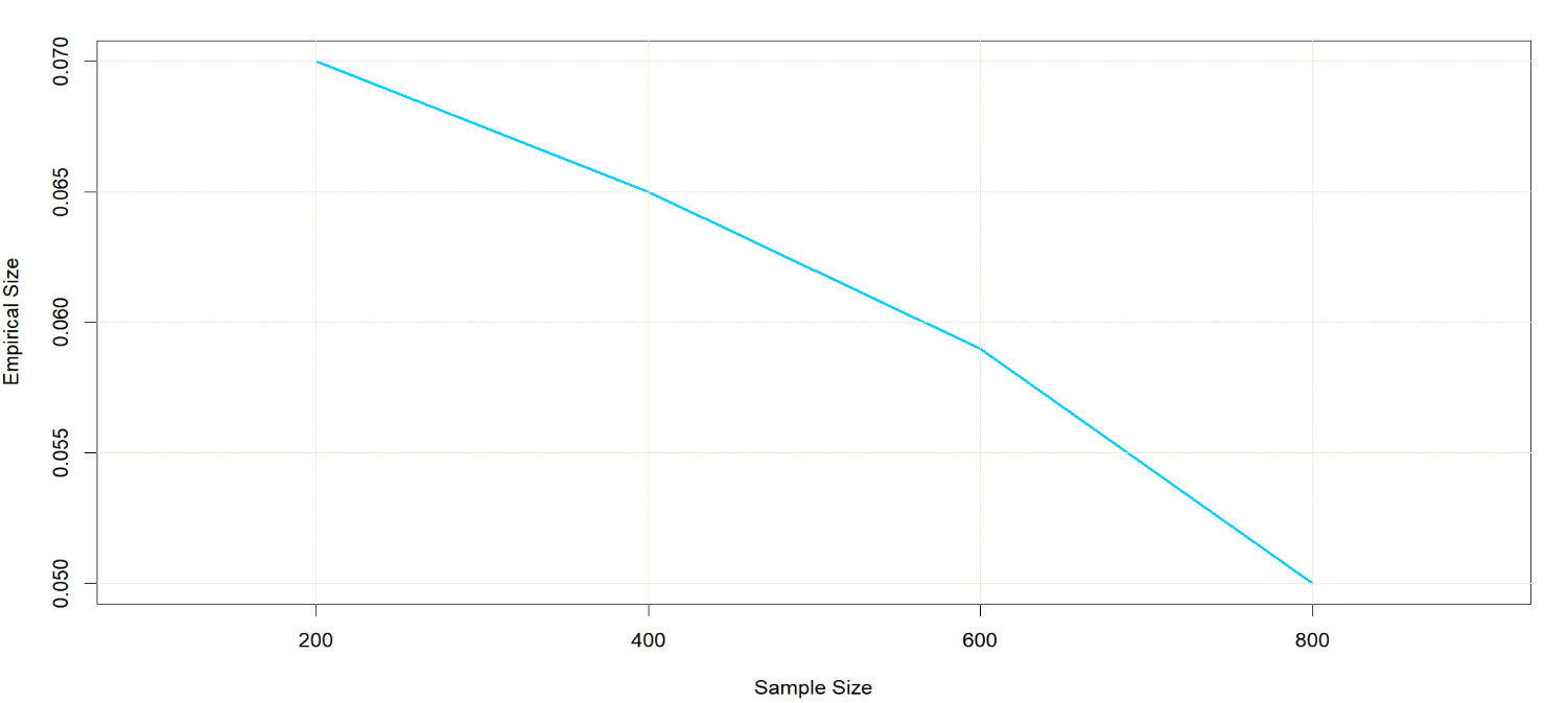
Figure 3: Relationship between Empirical size and Sample size when testing $H_{0}$ using the SS Technique and the Combined test statistic $\mathrm{TS}$ with $\alpha=0.05.$

Table 4: Empirical Rejection Probabilities Using the Individual test statistics $\mathrm{TS}_{k}$’s when $H_{0}$ is true and false with $\alpha=0.05.$

Normal Log-normal Techniques $\sigma_{\tau}$ $\Pr(\widehat{pval}_{0}<\alpha)$ $\Pr(\widehat{pval}_{1}<\alpha)$ FWER $\Pr(\widehat{pval}_{0}<\alpha)$ $\Pr(\widehat{pval}_{1}<\alpha)$ FWER $0.0$ $0.050$ $0.049$ $0.096$ $0.054$ $0.055$ $0.107$ $0.5$ $0.472$ $0.445$ $0.708$ $0.130$ $0.119$ $0.230$ Oracle $1.0$ $0.850$ $0.869$ $0.979$ $0.237$ $0.261$ $0.443$ $1.5$ $0.962$ $0.969$ $0.999$ $0.373$ $0.408$ $0.624$ $2.0$ $0.996$ $0.997$ $1.000$ $0.507$ $0.503$ $0.755$ $0.0$ $0.050$ $0.050$ $0.097$ $0.072$ $0.058$ $0.127$ $0.5$ $0.476$ $0.454$ $0.718$ $0.198$ $0.129$ $0.294$ Plug-in $1.0$ $0.850$ $0.858$ $0.976$ $0.391$ $0.260$ $0.549$ $1.5$ $0.961$ $0.958$ $0.999$ $0.579$ $0.407$ $0.743$ $2.0$ $0.993$ $0.996$ $1.000$ $0.721$ $0.492$ $0.855$ $0.0$ $0.025$ $0.035$ $0.058$ $0.051$ $0.049$ $0.098$ $0.5$ $0.400$ $0.394$ $0.639$ $0.122$ $0.112$ $0.216$ CI $1.0$ $0.822$ $0.819$ $0.965$ $0.223$ $0.242$ $0.415$ $1.5$ $0.950$ $0.951$ $0.996$ $0.346$ $0.382$ $0.591$ $2.0$ $0.991$ $0.993$ $1.000$ $0.476$ $0.455$ $0.710$ $0.0$ $0.044$ $0.053$ $0.096$ $0.077$ $0.062$ $0.134$ $0.5$ $0.224$ $0.217$ $0.380$ $0.166$ $0.098$ $0.243$ SS $1.0$ $0.527$ $0.501$ $0.762$ $0.356$ $0.182$ $0.466$ $1.5$ $0.711$ $0.716$ $0.925$ $0.496$ $0.272$ $0.619$ $2.0$ $0.852$ $0.851$ $0.980$ $0.623$ $0.356$ $0.751$

Estimates are based on 1000 replications, with a simulation standard error of 0.00689 under $H_{0}.$

Table 5: Empirical Rejection Probabilities Using the Combined test statistic $TS$ when $H_{0}$ is true and false with $\alpha=0.05.$

Techniques $\sigma_{\tau}$ Normal Log-normal 0.0    0.048    0.052 0.5    0.633    0.128 Oracle 1.0    0.975    0.295 1.5    0.998    0.459 2.0    1.000    0.618 0.0    0.047    0.061 0.5    0.635    0.161 Plug-in 1.0    0.973    0.387 1.5    0.998    0.552 2.0    1.000    0.704 0.0    0.030    0.043 0.5    0.557    0.118 CI 1.0    0.966    0.269 1.5    0.998    0.421 2.0    1.000    0.570 0.0    0.049    0.070 0.5    0.277    0.157 SS 1.0    0.642    0.300 1.5    0.856    0.406 2.0    0.941    0.509

Estimates are based on 1000 replications, with a simulation standard error of 0.00689 under $H_{0},$

Next, we shift attention to the null hypothesis $H_{0}^{\Pi}.$ Here, we first set $\psi_{0}=1,\psi_{1}=0,$ $N=200,$ and $\epsilon=0.20.$ To compute the rejection probability under the null hypothesis, we also set $\sigma_{\tau}=0$. Using the test statistics $\mathrm{TS}_{k}$ defined in (14), we report the rejection probabilities at a $5\%$ significance level under the normal and log-normal DGPs in Table 6. As in Table 4, the CI technique is valid but has a relatively lower size under both DGPs.

In Table 7, we report the rejection probabilities by applying the combined test statistic of $H_{0}^{\Pi}$. We set the same model parameters we used for the multiple test statistics. The results reveal the validity of the testing procedures under both DGPs and both techniques. Again, note that the slight over-rejections for the log-normal DGP under $H_{0}^{\Pi}$ when we deploy the SS technique is due to the small effective sample size.

Table 6: Empirical Rejection Probabilities Using the Individual test statistics $\mathrm{TS}_{k}$’s when $H^{\Pi}_{0}$ is true and false with $\alpha=0.05.$

Normal Log-normal Techniques $\sigma_{\tau}$ $\Pr(\widehat{pval}_{0}<\alpha)$ $\Pr(\widehat{pval}_{1}<\alpha)$ FWER $\Pr(\widehat{pval}_{0}<\alpha)$ $\Pr(\widehat{pval}_{1}<\alpha)$ FWER $0.0$ $0.050$ $0.049$ $0.096$ $0.054$ $0.055$ $0.107$ $0.5$ $0.472$ $0.445$ $0.708$ $0.130$ $0.119$ $0.230$ Oracle $1.0$ $0.850$ $0.869$ $0.979$ $0.237$ $0.261$ $0.443$ $1.5$ $0.962$ $0.969$ $0.999$ $0.373$ $0.408$ $0.624$ $2.0$ $0.996$ $0.997$ $1.000$ $0.507$ $0.503$ $0.755$ $0.0$ $0.051$ $0.053$ $0.102$ $0.068$ $0.062$ $0.128$ $0.5$ $0.469$ $0.454$ $0.712$ $0.151$ $0.149$ $0.275$ Plug-in $1.0$ $0.849$ $0.857$ $0.979$ $0.282$ $0.301$ $0.499$ $1.5$ $0.960$ $0.965$ $0.999$ $0.422$ $0.448$ $0.682$ $2.0$ $0.996$ $0.994$ $1.000$ $0.554$ $0.549$ $0.806$ $0.0$ $0.022$ $0.034$ $0.054$ $0.051$ $0.049$ $0.098$ $0.5$ $0.389$ $0.385$ $0.625$ $0.122$ $0.112$ $0.217$ CI $1.0$ $0.817$ $0.812$ $0.963$ $0.220$ $0.243$ $0.415$ $1.5$ $0.948$ $0.947$ $0.995$ $0.342$ $0.381$ $0.589$ $2.0$ $0.991$ $0.993$ $1.000$ $0.465$ $0.450$ $0.701$ $0.0$ $0.040$ $0.054$ $0.093$ $0.064$ $0.073$ $0.132$ $0.5$ $0.225$ $0.216$ $0.378$ $0.119$ $0.114$ $0.212$ SS $1.0$ $0.528$ $0.493$ $0.761$ $0.235$ $0.239$ $0.415$ $1.5$ $0.700$ $0.710$ $0.923$ $0.356$ $0.339$ $0.557$ $2.0$ $0.841$ $0.850$ $0.977$ $0.437$ $0.440$ $0.670$

Estimates are based on 1000 replications, with a simulation standard error of 0.00689 under $H^{\Pi}_{0}.$

Table 7: Empirical Rejection Probabilities Using the Combined test statistic $TS$ when $H^{\Pi}_{0}$ is true and false with $\alpha=0.05.$

Techniques $\sigma_{\tau}$ Normal Log-normal 0.0    0.048    0.052 0.5    0.633    0.128 Oracle 1.0    0.975    0.295 1.5    0.998    0.459 2.0    1.000    0.618 0.0    0.048    0.067 0.5    0.632    0.150 Plug-in 1.0    0.972    0.363 1.5    0.998    0.510 2.0    1.000    0.665 0.0    0.031    0.045 0.5    0.556    0.117 CI 1.0    0.953    0.271 1.5    0.998    0.412 2.0    1.000    0.566 0.0    0.046    0.067 0.5    0.273    0.148 SS 1.0    0.634    0.276 1.5    0.847    0.378 2.0    0.941    0.473

Estimates are based on 1000 replications, with a simulation standard error of 0.00689 under $H^{\Pi}_{0}.$

Lastly, we also numerically study the properties of the test of $H_{0}^{X,\Pi}.$ For this exercise, we set $\psi_{0}=1$ $\psi_{1}=1,$ and $\epsilon=0.1.$ To compute the rejection probability when $H_{0}^{X,\Pi}$ is true, we also set $\sigma_{\tau}=0$. We set the sample size to $400$ to ensure sufficient units for each subgroup defined by the covariate, treatment, and exposure. Using the test statistics $\mathrm{TS}_{k,l},$ we report the rejection probabilities at a $5\%$ significance level under the normal and log-normal DGPs in Table 8. The tests are valid under both DGPs and for both techniques. Also, in Table 9, we report the rejection probabilities using the combined test statistic $\mathrm{TS}^{X,\Pi},$ with the same parameters as in Table 8. Analogous to the other nulls, the results corroborate the validity of the testing procedures.

Table 8: Empirical Rejection Probabilities Using the Individual test statistics $\mathrm{TS}_{k,l}$’s when $H^{X,\Pi}_{0}$ is true and false with $\alpha=0.05.$ NB: $\widehat{pval}_{kl}=\hat{p}_{kl}.$

Normal Log-normal Techniques $\sigma_{\tau}$ $\Pr(\hat{p}_{00}<\alpha)$ $\Pr(\hat{p}_{10}<\alpha)$ $\Pr(\hat{p}_{01}<\alpha)$ $\Pr(\hat{p}_{11}<\alpha)$ FWER $\Pr(\hat{p}_{00}<\alpha)$ $\Pr(\hat{p}_{10}<\alpha)$ $\Pr(\hat{p}_{01}<\alpha)$ $\Pr(\hat{p}_{11}<\alpha)$ FWER $0.0$ $0.044$ $0.052$ $0.044$ $0.045$ $0.173$ $0.044$ $0.050$ $0.056$ $0.056$ $0.197$ Oracle $1.0$ $0.870$ $0.862$ $0.858$ $0.888$ $1.000$ $0.239$ $0.233$ $0.291$ $0.242$ $0.702$ $0.0$ $0.045$ $0.053$ $0.042$ $0.046$ $0.174$ $0.060$ $0.062$ $0.066$ $0.061$ $0.234$ Plug-in $1.0$ $0.865$ $0.851$ $0.839$ $0.852$ $1.000$ $0.290$ $0.277$ $0.335$ $0.275$ $0.761$ $0.0$ $0.024$ $0.038$ $0.027$ $0.029$ $0.113$ $0.041$ $0.045$ $0.053$ $0.050$ $0.182$ CI $1.0$ $0.829$ $0.795$ $0.808$ $0.796$ $0.999$ $0.216$ $0.219$ $0.265$ $0.220$ $0.659$ $0.0$ $0.055$ $0.058$ $0.064$ $0.056$ $0.210$ $0.088$ $0.082$ $0.082$ $0.077$ $0.298$ SS $1.0$ $0.551$ $0.531$ $0.529$ $0.523$ $0.953$ $0.265$ $0.255$ $0.222$ $0.231$ $0.667$

Estimates are based on 1000 replications, with a simulation standard error of 0.00689 under $H^{X,\Pi}_{0}.$

Table 9: Empirical Rejection Probabilities Using the Combined test statistic $\mathrm{TS}^{X,\Pi}$ when $H^{X,\Pi}_{0}$ is true and false with $\alpha=0.05.$

Techniques $\sigma_{\tau}$ Normal Log-normal 0.0 0.047    0.043 Oracle 1.0 1.000    0.383 0.0 0.047    0.066 Plug-in 1.0 1.000    0.457 0.0 0.012    0.051 CI 1.0 0.992    0.299 0.0 0.041    0.061 SS 1.0 0.820    0.320

Estimates are based on 1000 replications, with a simulation standard error of 0.00689 under $H^{X,\Pi}_{0}.$

5 Empirical Application

In this section, we use a subset of the experimental data from Cai et al. (2015) to demonstrate the usage of our proposed testing procedures. The experiment was implemented to help determine whether farmers’ understanding of a weather insurance policy affects purchasing decision. The authors examine the impact of two types of information sessions on insurance adoption among 4902 households in 173 small rice-producing villages (47 administrative villages) in 3 regions in the Jiangxi province in China. They show that the type of information session has direct effects on participants’ adoption and significant effects on the adoption decision of participants’ friends.

Figure 4: Links between households in the 47 villages. Different Villages have different colors. Adapted from Bargagli Stoffi et al. (2020)

The data includes each household’s network information as well as additional pre-treatment information such as age, gender, rice production area, risk aversion score, the fraction of household income from rice production, etc. The outcome of interest is binary: whether or not a household buys the insurance policy. Since each household can name at most 5 friends, as a directed network, Assumption 2 holds. For each village in the experiment, there were two rounds of information sessions offered to introduce the insurance product. In each round, two sessions were held simultaneously: a simple session (with less information) and an intensive session. Since the second round information sessions were held three days after the first, the delay between the two sessions was sufficiently long that farmers had time to communicate with friends, but not long enough that all the information from the first round session diffused across the whole population through friends of friends. Therefore, Assumption 1 is also satisfied. Table 10 shows the result of a logit regression of the insurance adoption on "Second-round"- a binary variable which is 1 if households participated in the second round session and 0 otherwise- among households participating in the simple sessions. The coefficients of "Second-round" indicate that the probability of adoption among the second-round participants in the simple sessions is higher than those of their first-round counterparts. We conjecture that this is evidence of information spillover.

Table 10: Logit Regression Evidence of Information spillover

	Dependent variable:
	Insurance takeup
	(Without village fixed effects)	(With village fixed effects)
Constant	$-$0.609∗∗∗	0.693
	(0.064)	(0.875)
Second-round	0.423∗∗∗	0.474∗∗∗
	(0.084)	(0.089)
Observations	2,453	2,453
Log Likelihood	$-$1,646.452	$-$1,546.740
Akaike Inf. Crit.	3,296.904	3,189.480
Note:	∗p$<$0.1; ∗∗p$<$0.05; ∗∗∗p$<$0.01

The analyses in Cai et al. (2015) also suggest that while farmers are influenced by their friends who attended the first round intensive sessions, they are not affected by friends who attended the first round simple sessions. Finally, they also show that people are less influenced by their friends when they have direct (same) education about the insurance products (i.e., information from first-round units in the intensive session does not affect the purchasing decision of second-round units in the intensive session).

To demonstrate the proposed testing procedures in our paper, we focus on three large villages - Dukou, Yazhou, and Yongfeng - with 502 households. This is the same sub-sample used in Wang et al. (2023). Note we are able to focus on a subset of villages and their network because of the clustered nature of the network as in display in Figure 4.

A specification test of the interference structure in Hoshino and Yanagi (2023) suggests that the correct network exposure mapping for this data set is $\pi_{i}(\mathbf{T}):=\mathbbm{I}(\sum_{j=1}^{N}T_{j}D_{j}A_{ij}/\sum_{j=1}^{N}D_{j}A_{ij}\geq 0).$ The treatment indicator variable $T$ is one if a household attended the intensive session and zero otherwise. Similarly, $D$ is a binary variable which is one if a household attended the first round session and zero otherwise. To test the null hypothesis $H_{0}^{X,\Pi}$, we use a balanced pretreatment variable insurance_repay which is also binary (equals 1 if a household has received a payout from other insurance before and zero otherwise).

Although the original randomization was stratified using two pretreatment variables, to ensure that we have sufficient units in each stratum in our subsample, we construct the strata using only one of those variables, household size.

Table 11: Test of $H_{0}$ at a $0.05$ significant level

                                                                 Multiple                                                          Combined Techniques $\epsilon$ $\Pr(\widehat{pval}_{0}<\alpha)$ $\Pr(\widehat{pval}_{1}<\alpha)$ $\Pr(\widehat{pval}<\alpha)$ 0.05 0.725 0.564 0.886 0.06 0.940 0.933 0.980 CI 0.07 0.873 0.758 0.624 0.08 0.604 0.933 1.000 0.05 0.483 0.987 0.168 0.06 0.235 0.973 0.819 SS 0.07 0.966 0.792 0.235 0.08 0.604 0.933 0.960

Table 12: Test of $H^{\Pi}_{0}$ at a $0.05$ significant level

                                                                 Multiple                                                           Combined Techniques $\epsilon$ $\Pr(\widehat{pval}_{0}<\alpha)$ $\Pr(\widehat{pval}_{1}<\alpha)$ $\Pr(\widehat{pval}<\alpha)$ 0.05 0.745 0.651 0.946 0.06 0.934 0.967 0.980 CI 0.07 0.873 0.832 0.705 0.08 0.644 0.967 1.000 0.05 0.483 0.987 0.154 0.06 0.235 0.973 0.866 SS 0.07 0.966 0.792 0.262 0.08 0.792 0.953 0.973

Table 13: Test of $H^{X,\Pi}_{0}$ at a $0.05$ significant level. NB: $\widehat{pval}_{kl}=\hat{p}_{kl}.$

                                                                                                                         Multiple                                                                           Combined Techniques $\epsilon$ $\Pr(\hat{p}_{00}<\alpha)$ $\Pr(\hat{p}_{10}<\alpha)$ $\Pr(\hat{p}_{01}<\alpha)$ $\Pr(\hat{p}_{11}<\alpha)$ $\Pr(\hat{p}<\alpha)$ 0.01 0.940 0.309 0.826 1.000 0.967 0.02 0.416 0.269 0.980 0.832 1.000 CI 0.03 1.000 0.987 0.960 0.665 0.993 0.04 0.946 0.893 1.000 0.812 0.839

Tables 11-13 reports the p-values of the test for $H_{0}$, $H^{\Pi}_{0}$ and $H^{X,\Pi}_{0}$ respectively. In each table, we display the p-values (at a $5\%$ significant level) using the two test statistics and our proposed techniques to handle nuisance parameters. For robustness, we also report the p-values at different values of the tuning parameter $\epsilon.$ From Table 11, we fail to reject the null hypothesis of constant treatment effect across the population. Both test statistics (testing approaches) and techniques assert that the effect of the type of information session on the decision to buy the weather insurance policy does not vary across households. Based on the decision from the test of $H_{0},$ we should also fail to reject $H^{\Pi}_{0}$ and $H^{X,\Pi}_{0}.$ Our results in Tables 12-13 corroborate this decision.

6 Conclusion

This paper proposes randomization tests for heterogeneous treatment effects when units interact on a single network. Applying the concept of network exposure mapping, the paper models network interference in the potential outcomes framework and considers several non-sharp null hypotheses that represent different notions of homogeneous treatment effects. We propose a conditional randomization inference method to deal with the presence of multiple potential outcomes and two procedures to overcome nuisance parameter issues. Overall, this paper offers insights for researchers seeking to infer heterogeneous treatment effects in a networked environment.

We may consider a few possible extensions. It is interesting to investigate goodness-of-fit test statistics like the Kolmogorov-Smirnov (KS) test statistic. In particular, can we extend the martingale transformation method applied to the KS test statistic by Chung and Olivares (2021)? Our immediate conjecture is that it is impossible without modifications due to the dependencies in network data sets. It is also interesting to extend the sample splitting technique to account for the randomness emanating from splits. A natural extension is a cross-fitting routine where we consider multiple independent splits of the data to approximate the distribution of the splits. Finally, it is worthwhile to extend our framework to allow for continuous pretreatment variables in the framework. Kernel-based estimators of the conditional variances and means can be employed in such settings. However, asymptotic properties of such estimators for graph depend random variables may pose a challenge.

7 Acknowledgments

This is a revised version of the second Chapter of my Ph.D. Dissertation at McMaster University, Owusu (2023). I am immensely grateful for the support and continuous advice of Youngki Shin, Jeffrey S. Racine, and Micheal Veall. Also, I wish to thank Saraswata Chaudhuri, Thomas M. Russell, Sukjin Han, David Pacini, seminar participants at the 57th Annual Conference of the Canadian Economics Association and the University of Exeter Econometrics seminar participants at for helpful comments. All errors are my own.

8 Appendix

Randomization Versus Permutation Tests

A permutation test is nonparametric test that involves randomly re-assigning the labels of the variable of interest of the observed data to generate a null distribution. Permutation tests solely rely on the assumption of exchangeability. Hence, they are suitable for testing hypotheses where the null implies exchangeability of some known transformation of the data. In addition, data can be observational. An advantage of the testing procedure using the conditioning procedure described in Section 3 .2 and the sample splitting technique in Section 3 .3.1 is that tests for the null hypotheses under consideration can be implemented as a permutation test. It involves the following steps.

1. Split the sample into two balanced subsample as in Section 3 .2.

2. Use the estimation sample to estimate the nuisance parameter.

3. Select the super focal units based on the observed exposure variable from the inference sample.

4. Compute the observed test statistic using the super focal units.

5. Suppose the null hypothesis is true and permute the super focal units a sufficient number of times to generate the distribution of the test statistic under the null hypothesis.

6. Compute the p-value using the observed test statistic and the test statistics obtained from the permutations.

Unlike the randomization test, the permutation testing procedure uses the super focal units solely as the conditioning event. Note that the permutation testing procedure is also not valid in finite samples since we have to estimate the nuisance parameter using the estimation sample. However the procedure is valid asymptotically.

By design, the permutation testing procedure generates a null distribution of the test statistic that has a lower variance compared to the randomization testing procedure. This is due to the fact that it is possible to obtain the same value of the test statistic under different permutations of the outcome variable (adjusted by the nuisance parameter). The following Proposition, summarizes the the difference between the permutation testing procedure we describe and randomization testing procedure.

Proposition 1.

Let $z(\mathbf{Y}^{obs},\mathbf{T},\mathbf{X},\mathbf{A})$ be a generic test statistic such that $\mathbbm{E}[z(\mathbf{Y}^{obs},\mathbf{T},\mathbf{X},\mathbf{A})]=0.$ Then, for the null hypothesis $H_{0}^{G},$ the upper bound of the p-values using the permutation testing procedure is less than the upper bound of the p-values using the randomization testing procedure. As such, the permutation test is more likely to over reject the null hypothesis leading to higher size.

Using Chebyshev’s inequality, we prove Proposition 1 in Appendix Lemmas and Proofs. In practice, for large samples, the p-values will coincide since we use a random sample of the permuted outcomes and permuted treatments to generate the null distribution.

Lemmas and Proofs

To prove the main theoretical results, we need the following Lemma.

Lemma 1 (The probability integral transform theorem).

Assume a random variable $A$ has a continuous distribution for which the cumulative distribution function (CDF) is $F_{A}$. Then, the random variable $B$ defined as $B=F_{A}(A)$ has a standard uniform distribution.

.1 Proof of Theorem 1 (i)

Proof.

For any $k,$ and for any treatment vector $\Lambda(\mathbf{T})\in\mathcal{T}_{k},$ the p-value is

$$pval_{{}_{k}}(\mathbf{T},\mathbf{Y}^{obs};\mathcal{T}_{k},F_{k},F_{k}^{obs})= \Pr(\mathrm{TS}_{k}(\mathbf{Y}_{F_{k}}(\Lambda(\mathbf{T})),\Lambda(\mathbf{T}),\mathbf{A};\mathcal{T}_{k},F_{k})\geq\mathrm{TS}_{k}(\mathbf{Y}^{obs},\mathbf{t}^{obs},\mathbf{A};F_{k}^{obs})|H_{0})$$

Since the test statistics are functions of estimated variances, i.e.,

$$\mathrm{TS}_{k}=\omega(\hat{\sigma}^{2}_{0}(\pi_{k}),\hat{\sigma}^{2}_{1}(\pi_{k})),$$

the asymptotic distribution of the test statistics depends on the asymptotic distribution of the conditional variances $\hat{\sigma}^{2}_{t}(\pi_{k}).$ Therefore, to study the asymptotic properties of the observed and permuted test statistics, we study the asymptotic properties of the conditional variances estimated using the observed and permuted data (data after permuting the treatment assignment vector) respectively.

First, Let us focus on the conditional variances estimated using the observed subsample of super focal units

$$\hat{\sigma}^{2}_{t}(\pi_{k}):=\frac{\sum_{i=1}^{N}(Y^{obs}_{i}-\bar{Y}_{tk}^{obs})^{2}\cdot\mathbbm{I}(T_{i}=t)\cdot\mathbbm{I}(F_{ik}^{obs}=1)}{\sum_{i=1}^{N}\mathbbm{I}(T_{i}=t)\cdot\mathbbm{I}(F_{ik}^{obs}=1)-1},$$ (.1)

where $\bar{Y}_{tk}^{obs}$ denotes the conditional sample mean and $F_{ik}^{obs}$ is an indicator variable that equals to 1 if unit $i$ is part of the random sample from the super focal units selected to compute the conditional variance or 0 otherwise. $F_{ik}^{obs}$ is well defined in Remark 1.

Next, we look at the conditional variances estimated using the permuted data for an arbitrary permutation $\Lambda(\mathbf{T})$ of the the treatment assignment vector.

$$\tilde{\sigma}^{2}_{t}(\pi_{k}):= \frac{\sum_{i=1}^{N}(\Lambda(Y_{i})^{obs}-\Lambda(\bar{Y}_{tk})^{obs})^{2}\cdot\mathbbm{I}(\pi_{i}(\mathbf{T})=\pi_{k})\cdot\mathbbm{I}(\Lambda(T_{i})=t)\cdot\mathbbm{I}(\pi_{i}(\Lambda(\mathbf{T}))=\pi_{k})}{\sum_{i=1}^{N}\mathbbm{I}\{\Lambda(T_{i})=t,\pi_{i}(\mathbf{T})=\pi_{k},\pi_{i}(\Lambda(\mathbf{T}))=\pi_{k}\}-1}$$ (.2)

$$= \frac{\sum_{i=1}^{N}(\Lambda(Y_{i})^{obs}-\Lambda(\bar{Y}_{tk})^{obs})^{2}\cdot\mathbbm{I}(\Lambda(T_{i})=t)\cdot\mathbbm{I}(F_{ik}(\Lambda(\mathbf{T}))=1)}{\sum_{i=1}^{N}\mathbbm{I}(\Lambda(T_{i})=t)\cdot\mathbbm{I}(F_{ik}(\Lambda(\mathbf{T}))=1)-1},$$ (.3)

where $\Lambda(\bar{Y}_{tk})^{obs}$ denotes the conditional sample mean when treatment assignment is $\Lambda(\mathbf{T}).$

Note that

$$\Pr(T_{i}=t)=\Pr(\Lambda(T_{i})=t),\,\,\forall t=0,1,$$

since the permutations of treatment assignment respects the treatment assignment mechanism. In addition,

$$\Pr(\pi_{i}(\mathbf{T})=\pi_{k})=\Pr(\pi_{i}(\Lambda(\mathbf{T}))=\pi_{k}),\,\,\forall k=1\,\dots K,$$

since the network is exogenous. Also, the distribution of outcomes are invariant to the permutations of the treatment assignment vector.

Therefore, comparing the estimators in (.1) and (.3), their distribution only differ by the indicator variables $F^{obs}_{ik}$ and $F_{ik}(\Lambda(\mathbf{T})).$ However, since $F^{obs}_{ik}$ is such that $\sum_{i=1}^{N}F^{obs}_{ik}=\mathbbm{E}[\sum_{i=1}^{N}F_{ik}(\Lambda(\mathbf{T}))]=N\mathbbm{E}[F_{ik}(\Lambda(\mathbf{T}))]$ (from Remark 1), and the fact that under Assumption 3, the weak law of large numbers for graph dependent random variables holds, i.e.,

$$\lim_{N\to\infty}\sum_{i=1}^{N}F_{ik}(\Lambda(\mathbf{T}))=N\mathbbm{E}[F_{ik}(\Lambda(\mathbf{T}))],$$

the asymptotic distributions of $\hat{\sigma}^{2}_{t}(\pi_{k})$ and $\tilde{\sigma}^{2}_{t}(\pi_{k})$ are equivalent.

Now, let $G_{k}$ denote the asymptotic null distribution of $-\mathrm{TS}_{k}(\mathbf{Y}_{F_{k}}(\Lambda(\mathbf{T})),\Lambda(\mathbf{T}),\mathbf{A};\mathcal{T}_{k},F_{k})$ for any treatment vector $\Lambda(\mathbf{T})\in\mathcal{T}_{k}$ , then the p-value at the limit is

$$\lim_{N\to\infty}pval_{{}_{k}}(\mathbf{T},\mathbf{Y}^{obs};\mathcal{T}_{k},F_{k},F_{k}^{obs})=G_{k}(-\mathrm{TS}_{k}(\mathbf{Y}^{obs},\mathbf{T}^{obs},\mathbf{A};F_{k}^{obs})).$$

Because the test statistic depend on the conditional variances, note that the asymptotic distribution of $-\mathrm{TS}_{k}(\mathbf{Y}_{F_{k}}(\Lambda(\mathbf{T})),\Lambda(\mathbf{T}),\mathbf{A};\mathcal{T}_{k},F_{k})$ coincides with that of the observed test statistic. Specifically, for a large sample size, the observed test statistic $-\mathrm{TS}_{k}(\mathbf{Y}^{obs},\mathbf{T}^{obs},\mathbf{A};F_{k}^{obs})$ also has the asymptotic null distribution $G_{k}.$

Now, from Lemma 1, $pval_{{}_{k}}(\mathbf{T},\mathbf{Y}^{obs};\mathcal{T}_{k},F_{k})$ has a standard uniform distribution in the limit and as such,

$$\lim_{N\to\infty}\Pr(pval_{{}_{k}}(\mathbf{T},\mathbf{Y}^{obs};\mathcal{T}_{k},F_{k})\leq\alpha)\leq\alpha\,\,\text{for any}\,\,\alpha\in[0,1]$$ (.4)

as required. Note that we do not achieve strict equality in inequality (.4) (as Lemma 1 suggests) due to the fact that the test statistics are discrete in $\mathcal{T}_{k}.$ ∎

.2 Proof of Theorem 2(i)

Proof.

Let $\mathcal{U}^{est}$ and $\mathcal{U}^{inf}$ be a random equal split of the data into estimation and inference sub-samples. Now, let $\hat{\tau}^{est}$ be an estimator of the average treatment effect conditional on the sub-sample $\mathcal{U}^{est}.$ Assume that $\hat{\tau}^{est}$ is a consistent estimator of the unconditional sample average treatment effect $\tau.$

Next, for any $k,$ let $G_{k|\hat{\tau}^{est}}$ denote the asymptotic distribution of $-\mathrm{TS}_{k}(\mathbf{Y}_{F_{k}}(\Lambda(\mathbf{T})),\Lambda(\mathbf{T}),\mathbf{A};\mathcal{T}_{k},F_{k},\hat{\tau}^{est}).$ Note that this distribution is conditional on a given balanced sample split and the conditioning mechanism. Therefore, the probability is with respect to the randomness of $\Lambda(\mathbf{T})\in\mathcal{T}_{k}^{\mathcal{U}^{inf}}$, where $\mathcal{T}_{k}^{\mathcal{U}^{inf}}$ is the subset of treatment assignment vectors of the inference sub-sample that meet the conditioning mechanism on the full sample.

Under the null hypothesis $H_{0}$, as $N\to\infty,$ from Theorem 1, the limit laws of the test statistics are invariant to permutations of the treatment assignment vector, i.e., $-\mathrm{TS}_{k}(\mathbf{Y}^{obs},\mathbf{T},\mathbf{A};F_{k}^{obs},\hat{\tau}^{est})$ also has an asymptotic distribution $G_{k|\hat{\tau}^{est}}.$ Therefore the p-value at the limit is

$$\lim_{N\to\infty}pval_{{}_{k}}(\mathbf{T},\mathbf{Y}^{obs};\mathcal{T}_{k},F_{k},F_{k}^{obs}\hat{\tau}^{est})= G_{k|\hat{\tau}^{est}}(-\mathrm{TS}_{k}(\mathbf{Y}^{obs},\mathbf{T}^{obs},\mathbf{A};\mathcal{T}_{k},F_{k},\hat{\tau}^{est}))$$

From Lemma 1, $pval_{{}_{k}}(\mathbf{T},\mathbf{Y}^{obs};\mathcal{T}_{k},F_{k},F_{k}^{obs},\hat{\tau}^{est})$ has a standard uniform distribution in the limit. Combining this fact with the consistency of the average treatment effect estimator using the estimation sample, we have

$$\lim_{N\to\infty}\Pr(pval_{{}_{k}}(\mathbf{T},\mathbf{Y}^{obs};\mathcal{T}_{k},F_{k},F_{k}^{obs},\hat{\tau}^{est})\leq\alpha)\leq\alpha\,\,\text{for any}\,\,\alpha\in[0,1]$$

as required. ∎

.3 Proof of Theorem 3 (i)

Proof.

Let $\tau_{0}$ be the true value of the nuisance parameter $\tau.$ Then,

$$\lim_{N\to\infty}\Pr(pval_{{}_{k,\gamma}}(\mathbf{T},\mathbf{Y}^{obs};\mathcal{T}_{k},F_{k},F_{k}^{obs})\leq\alpha|\,H_{0})= \lim_{N\to\infty}\Pr(pval_{{}_{k,\gamma}}(\mathbf{T},\mathbf{Y}^{obs};\mathcal{T}_{k},F_{k},F_{k}^{obs})\leq\alpha,\tau_{0}\in\mathrm{CI}_{\gamma}|\,H_{0})$$

$$+\lim_{N\to\infty}\Pr(pval_{{}_{k,\gamma}}(\mathbf{T},\mathbf{Y}^{obs};\mathcal{T}_{k},F_{k},F_{k}^{obs})\leq\alpha,\tau_{0}\notin\mathrm{CI}_{\gamma}|\,H_{0})$$

$$\leq \lim_{N\to\infty}\Pr\Bigg{(}\sup_{\tau^{\prime}\in\mathrm{CI}_{\gamma}}pval_{k}(\tau^{\prime})+\gamma\leq\alpha,\tau_{0}\in\mathrm{CI}_{\gamma}|\,H_{0}\Bigg{)}$$

$$+\lim_{N_{k}\to\infty}\Pr(\tau_{0}\notin\mathrm{CI}_{\gamma}|H_{0})$$

$$\leq \lim_{N\to\infty}\Pr(pval_{k}(\tau_{0})\leq\alpha-\gamma,\tau_{0}\in\mathrm{CI}_{\gamma}|\,H_{0})$$

$$+\lim_{N\to\infty}\Pr(\tau_{0}\notin\mathrm{CI}_{\gamma}|\,H_{0})$$

$$\leq \alpha-\gamma+\gamma=\alpha$$

The first equality is an application of the law of total probability. The first inequality is also a straightforward use of the relationship between marginal and joint probabilities for the second term. The second inequality uses the fact that $\sup_{\tau^{\prime}\in\mathrm{CI}_{\gamma}}pval_{k}(\tau^{\prime})$ stochastically dominates $pval_{k}(\tau_{0}).$ The last inequality uses Theorem 1 and the fact that $\mathrm{CI}_{\gamma}$ is a valid confidence interval. ∎

.4 Proof of Proposition 1

Proof.

Let $z(\mathbf{Y}^{obs},\mathbf{T},\mathbf{X},\mathbf{A})$ be a generic test statistic such that $\mathbbm{E}[z(\mathbf{Y}^{obs},\mathbf{T},\mathbf{X},\mathbf{A})]=0.$ Also, let $\Lambda(\mathbf{Y}^{obs})$ denote a permutation of the vector of observed outcomes. Then, applying Chebyshev’s inequality, the p-value using the permutation testing procedure is

$$\Pr(|z(\Lambda(\mathbf{Y}^{obs}),\mathbf{T},\mathbf{X},\mathbf{A})|\geq z(\mathbf{Y}^{obs},\mathbf{T},\mathbf{X},\mathbf{A})|H_{0}^{G})\leq\frac{\sigma^{2}_{p}}{z(\mathbf{Y}^{obs},\mathbf{T},\mathbf{X},\mathbf{A})^{2}},$$

where $\sigma^{2}_{p}$ is the variance of the test statistics obtained by permuting outcome. Analogously, the p-value using the randomization testing procedure is

$$\Pr(|z(\mathbf{Y}^{obs},\Lambda(\mathbf{T}),\mathbf{X},\mathbf{A})|\geq z(\mathbf{Y}^{obs},\mathbf{T},\mathbf{X},\mathbf{A})|H_{0}^{G})\leq\frac{\sigma^{2}_{r}}{z(\mathbf{Y}^{obs},\mathbf{T},\mathbf{X},\mathbf{A})^{2}},$$

where $\sigma^{2}_{r}$ is the variance of the test statistics obtained by permuting treatment. By design, $\sigma^{2}_{r}>\sigma^{2}_{p}.$ Hence the upper bound of the p-values using the permutation testing procedure is less than the upper bound of the p-values using the randomization testing procedure. ∎

References

- Aronow (2012) Aronow, P. M. (2012). A general method for detecting interference between units in randomized experiments. Sociological Methods & Research 41(1), 3–16.
- Aronow et al. (2017) Aronow, P. M., C. Samii, et al. (2017). Estimating average causal effects under general interference, with application to a social network experiment. The Annals of Applied Statistics 11(4), 1912–1947.
- Athey et al. (2018) Athey, S., D. Eckles, and G. W. Imbens (2018). Exact p-values for network interference. Journal of the American Statistical Association 113(521), 230–240.
- Bargagli Stoffi et al. (2020) Bargagli Stoffi, F., C. Tortú, and L. Forastiere (2020). Heterogeneous treatment and spillover effects under clustered network interference. Costanza and Forastiere, Laura, Heterogeneous Treatment and Spillover Effects Under Clustered Network Interference (August 3, 2020).
- Basse et al. (2019) Basse, G. W., A. Feller, and P. Toulis (2019). Randomization tests of causal effects under interference. Biometrika 106(2), 487–494.
- Berger and Boos (1994) Berger, R. L. and D. D. Boos (1994). P values maximized over a confidence set for the nuisance parameter. Journal of the American Statistical Association 89(427), 1012–1016.
- Bitler et al. (2006) Bitler, M. P., J. B. Gelbach, and H. W. Hoynes (2006). What mean impacts miss: Distributional effects of welfare reform experiments. American Economic Review 96(4), 988–1012.
- Cai et al. (2015) Cai, J., A. De Janvry, and E. Sadoulet (2015). Social networks and the decision to insure. American Economic Journal: Applied Economics 7(2), 81–108.
- Chung and Olivares (2021) Chung, E. and M. Olivares (2021). Permutation test for heterogeneous treatment effects with a nuisance parameter. Journal of Econometrics 225(2), 148–174.
- Cox (1958) Cox, D. R. (1958). Planning of experiments.
- Crump et al. (2008) Crump, R. K., V. J. Hotz, G. W. Imbens, and O. A. Mitnik (2008). Nonparametric tests for treatment effect heterogeneity. The Review of Economics and Statistics 90(3), 389–405.
- Ding et al. (2016) Ding, P., A. Feller, and L. Miratrix (2016). Randomization inference for treatment effect variation. Journal of the Royal Statistical Society: Series B: Statistical Methodology, 655–671.
- Fisher (1925) Fisher, R. (1925). Statistical methods for research workers (oliver and boyd, edinburgh, scotland), 299.
- Han et al. (2022) Han, S., J. Owusu, and Y. Shin (2022). Statistical treatment rules under social interaction. arXiv preprint arXiv:2209.09077.
- Hoshino and Yanagi (2023) Hoshino, T. and T. Yanagi (2023). Randomization test for the specification of interference structure. arXiv preprint arXiv:2301.05580.
- Isaki and Fuller (1982) Isaki, C. T. and W. A. Fuller (1982). Survey design under the regression superpopulation model. Journal of the American Statistical Association, 89–96.
- Lehmann and Romano (2022) Lehmann, E. and J. P. Romano (2022). The general decision problem. In Testing statistical hypotheses, pp. 3–28. Springer.
- Leung (2020) Leung, M. P. (2020). Treatment and spillover effects under network interference. Review of Economics and Statistics 102(2), 368–380.
- Liu and Hudgens (2014) Liu, L. and M. G. Hudgens (2014). Large sample randomization inference of causal effects in the presence of interference. Journal of the american statistical association 109(505), 288–301.
- Manski (2013) Manski, C. F. (2013). Identification of treatment response with social interactions. The Econometrics Journal 16(1), S1–S23.
- Owusu (2023) Owusu, J. (2023). Treatment Effect Heterogeneity and Statistical Decision-making in the Presence of Interference. Ph. D. thesis.
- Paluck et al. (2016) Paluck, E. L., H. Shepherd, and P. M. Aronow (2016). Changing climates of conflict: A social network experiment in 56 schools. Proceedings of the National Academy of Sciences 113(3), 566–571.
- Sant’Anna (2021) Sant’Anna, P. H. (2021). Nonparametric tests for treatment effect heterogeneity with duration outcomes. Journal of Business & Economic Statistics 39(3), 816–832.
- Sävje et al. (2021) Sävje, F., P. Aronow, and M. Hudgens (2021). Average treatment effects in the presence of unknown interference. Annals of statistics 49(2), 673.
- Viviano (2019) Viviano, D. (2019). Policy targeting under network interference. arXiv preprint arXiv:1906.10258.
- Wager and Athey (2018) Wager, S. and S. Athey (2018). Estimation and inference of heterogeneous treatment effects using random forests. Journal of the American Statistical Association 113(523), 1228–1242.
- Wang et al. (2023) Wang, J., P. Li, and F. Hu (2023). A/b testing in network data with covariate-adaptive randomization.
- Zhang and Zhao (2022) Zhang, Y. and Q. Zhao (2022). What is a randomization test? arXiv preprint arXiv:2203.10980.