Measurement of the astrophysical diffuse neutrino flux in a combined fit of IceCube’s high energy neutrino data

Abstract

The IceCube Neutrino Observatory has discovered a diffuse neutrino flux of astrophysical origin and measures its properties in various detection channels. With more than 10 years of data, we use multiple data samples from different detection channels for a combined fit of the diffuse astrophysical neutrino spectrum. This leverages the complementary information of different neutrino event signatures. For the first time, we use a coherent modelling of the signal and background, as well as the detector response and corresponding systematic uncertainties. The detector response is continuously varied during the simulation in order to generate a general purpose Monte Carlo set, which is central to our approach. We present a combined fit yielding a measurement of the diffuse astrophysical neutrino flux properties with unprecedented precision.

Corresponding authors: Richard Naab^1∗, Erik Ganster², Zelong Zhang^3
1 DESY Zeuthen
² RWTH Aachen University
³ Stony Brook University
^∗ Presenter

1 Introduction

A high-energy astrophysical neutrino flux was discovered by IceCube in 2013 [1], and has subsequently been characterized using several neutrino detection channels such as high energy starting events [2], through-going muon tracks [3] and cascades [4]. The astrophysical neutrino flux has been well-described by an unbroken single power law (SPL) so far; see Figure 1 for an overview of the measured properties. Hints for substructure in the spectrum, as seen in independent measurements [3] and [4], are so far statistically insignificant, however.

Previously, several data samples have been combined in a likelihood fit [5], thus enabling us to derive constraints from complementary data samples with different energy resolutions, sky coverage, and backgrounds. While this did result in an improved characterization of the astrophysical flux, not all uncertainties in the modeling were treated consistently: most notably, the energy scale was treated in an independent way between the samples, which increased the fit uncertainty significantly.

Here, we present a combined fit using IceCube’s track and cascade data, which for the first time uses a rigorously combined treatment of the detector response, as well as signal and background fluxes. The toolkit developed for such an analysis was previously verified, especially in terms of the treatment of detector systematic uncertainties [6, 7], and can be easily extended to include more data samples in the future.

2 Event samples

The combined fit presented here uses events from the cascade and through-going track sample, with the event selections outlined in more detail below. By combining these two channels we leverage the complementary information from these different neutrino event signatures: shower-like events in the cascade channel provide good energy resolution because most of the visible energy is deposited within the instrumented volume of the detector.

Only atmospheric $\nu_{\mu}$ neutral current (NC) events, as well as all atmospheric $\nu_{e}$ events, produce shower-like events. For these cascade event signatures, atmospheric neutrinos can be vetoed effectively by observing accompanying muons from air showers; this so-called "self-veto" technique further reduces background for down-going events, see [8] and references therein. The track sample, on the other hand, provides a much larger effective area since $\nu_{\mu}$ interacting far outside the instrumented volume can produce high-energy muons which leave a track-like signature in the detector. The angular resolution for these events is much better and enables the resolution of the zenith-dependent atmospheric flux properties.

Both samples were processed using IceCube Pass-2 re-processed data using the latest detector calibrations for all track and cascade data used within this analysis [9]. This allows for fitting both selections with a common set of nuisance parameters modeling not only the atmospheric flux uncertainties but also the detector systematic uncertainties in a common and unified way.

2.1 Track sample

The through-going muon track sample described and defined in [3] focuses on up-going track-like events with a reconstructed zenith angle $\theta_{\mathrm{reco}}>$85\text{\,}\mathrm{\SIUnitSymbolDegree}$$. This cut uses the Earth as a shield against the background of atmospheric muons reaching the IceCube in-ice neutrino detector. This background is further reduced by a boosted decision tree (BDT) trained to separate atmospheric muons from muons originating from charged current muon-neutrino interactions. The result is a high purity (>$99.8\text{\,}\mathrm{\char 37\relax}$) sample of muon neutrinos of either atmospheric or astrophysical origin [3]. One year of data taken with the partial 59-string configuration of IceCube is not included in our combined fit since it cannot be described in the otherwise uniform Monte Carlo modeling of the detector response. In the combined fit, we use 542066 selected track events.

2.2 Cascade sample

We select cascade data as described in [4], resulting in a full-sky sample. The selection differentiates low-level cascade events in low- and high-energy regimes, where the low-energy event selection mainly uses a BDT method and the high energy ($E_{\mathrm{reco}}>$60\text{\,}\mathrm{TeV}$$) event selection uses selection cuts on individual reconstructed event properties; see [4] and references therein. The event selection was updated in terms of using the Pass-2 re-processing described above and uses improved modeling [10] of glacial ice for the reconstruction of cascade events, and the data sample was extended until mid 2021. In the combined fit, we use 12641 selected cascade events.

In addition to using events classified as cascades for spectral measurement, the low-energy event selection also identifies a class of events with muons mimicking showers. This muon control sample is used to constrain the flux level in our background modeling. Moreover, the single-sample cascade analysis also uses classified starting track events mimicking showers identified in the low-energy selection. This constrains the contribution of NC $\nu_{\mu}$ events constituting the dominant background from the conventional atmospheric neutrino flux. This latter class of events is not included in the combined fit presented here.

3 Analysis methods

3.1 Detector response modeling and treatment of systematics

In order to model the detector response and corresponding uncertainties, we use the so-called StormStorm MC approach, as outlined in [11]. Detector response parameters which are uncertain are varied continuously on an event-by-event basis in the Monte Carlo simulation, populating the phase space in which the detector response parameters fall, which we constrain from calibration measurements. Contrary to the method proposed in [12], we extract gradients from the SnowStorm simulation set [11] and apply those to a separate Monte Carlo set simulated at nominal detector response parameters. This latter approach was verified in [6]. The detector response parameters taken into account in this analysis are those describing the bulk scattering and absorption coefficients of the glacial ice, the impact of the re-frozen drill holes as well as the efficiency of the optical sensors.

We use this Monte Carlo simulation consistently for estimating the observable distribution in all event selections, and we note that such an approach is central to the combined fit which has to take into account the correlations between the different event samples.

In order to simulate signal and background neutrino interaction events, we use the CSMS cross-section [13] and propagate secondary particles using [14], and its parametrization of the muon energy losses.

3.2 Background modelling

Table 1 lists all nuisance parameters used to model the background flux components in the combined fit. The atmospheric neutrino flux contributions are calculated using MCEq [15]. We use H4a as a primary cosmic ray flux model and Sibyll 2.3c as a hadronic interaction model as baseline, as well as an interpolation between the two primary cosmic ray models H4a and GST4 as in [3]; see also the references therein. Uncertainties on the conventional neutrino flux are taken into account following the scheme from Barr et al. [16], the corresponding nuisance parameters referred to as $\mathrm{Barr}\,X$, see [3] for detailed description of this as well as the muon template.

Modeling the effect of the atmospheric self-veto for the cascade selection is computationally challenging since, in principle, full air shower simulation including neutrino yields has to be produced to evaluate the effect of accompanying muons to atmospheric neutrinos. Since the event selections are typically very effective in terms of rejecting atmospheric muons, this becomes a hard problem, since most of the generated simulation will not pass the selection. In order to model the effect of the atmospheric self-veto, we use the MCEq atmospheric flux and muon range calculations employed in [8].

We note that the response to atmospheric muons is event selection specific. It is parameterized in terms of the veto probability as a function of the muon energy at detector entry. The self-veto effective threshold describing this response is hard to constrain due to the computational limitations explained above; we therefore leave it a free nuisance parameter in the fit.

Nuisance parameter	Allowed Range	Prior
Optical Efficiency	$[0.9,1.1]$	-
Bulk Ice Absorption	$[0.9,1.1]$	-
Bulk Ice Scattering	$[0.9,1.1]$	-
Hole-Ice $p_{0}$	$[-0.84,+0.3]$	-
Hole-Ice $p_{1}$	$[-0.134,+0.05]$	-
Self-veto Effective Threshold in GeV	$[5,2000]$	-
Conventional Flux Normalization	$[0.0,\infty)$	-
Prompt Flux Normalization	$[0.0,\infty)$	-
Muon Flux Normalization (cascades only)	$[0.0,\infty)$	-
Muon Template Normalization (tracks only)	$[0.0,\infty)$	-
Cosmic-Ray Model Interpolation	$[-1.0,+2.0]$	$\mathcal{G}(0.0,1.0)$
Cosmic-Ray Spectral Index Shift	$[-1.0,+1.0]$	-
Barr H	$[-0.8,+0.8]$	$\mathcal{G}(0.0,0.15)$
Barr W	$[-0.6,+0.6]$	$\mathcal{G}(0.0,0.4)$
Barr Y	$[-0.6,+0.6]$	$\mathcal{G}(0.0,0.3)$
Barr Z	$[-0.244,+0.6]$	$\mathcal{G}(0.0,0.12)$

Table 1: Nuisance parameters in the analysis, their allowed ranges, and Gaussian priors $\mathcal{G}(\mu,\sigma)$ (if used).

3.3 Signal modelling

For modeling the astrophysical neutrino flux multiple models of the spectral shape are tested. For all models, the astrophysical flux is assumed to be isotropic over the full sky with a flavor composition of $(\nu_{e}:\nu_{\mu}:\nu_{\tau})_{\mathrm{at\,Earth}}=(1:1:1)$ and equal ratio of $\nu/\bar{\nu}$ corresponding to idealized pp sources where neutrinos are produced from decays of $\pi^{\pm}$.

The tested spectral shapes include a single power-law (SPL) flux, a log-parabolic (LogP), and a broken power law (BPL) flux according to models A, C, and D in [4]. Also, a segmented flux model that assumes an $E^{-2}$ flux in individual neutrino energy bins with independent normalization each is used.

3.4 Likelihood fit

The analysis is performed with a forward-folding likelihood fit where the Monte Carlo events are weighted according to the parameters describing the signal and background fluxes as described above. We bin cascade and track data separately in the respective reconstructed energy and zenith observables, in order to resolve spectral features and discriminate the isotropic astrophysical neutrino flux from the atmospheric backgrounds with different zenith dependencies. We take into account the limited amount of Monte Carlo simulation statistics, due to computational limitations, in terms of using the effective likelihood described in [17]. The analysis bins in the combined fit are de-correlated by removing all overlapping events from the tracks sample - these are a minor fraction of starting events that are not relevant to the sensitivity of this measurement [12]. We note that this de-correlation can only be achieved using the general-purpose MC simulation developed for the purpose of this work.

In order to perform the fit, $\mathcal{O}(10^{7})$ Monte Carlo events have to be re-weighted at every minimizer iteration. In order to do this computationally efficiently, we use aesara [18] allowing for fast evaluation of mathematical expressions involving multi-dimensional arrays as well as efficient symbolic differentiation, which we use to provide gradients of the likelihood function to the minimizer.

4 Results

We find good agreement between data and Monte Carlo in the combined fit, see Figure 2. This agreement was tested extensively in the background region below 10 TeV in reconstructed energy to ensure correct combined modeling of the region where the atmospheric fluxes dominate.

In the region of the spectrum where the astrophysical flux dominates, we see structures deviating from a SPL. Notably, we see an excess of data at around 20-30 TeV in reconstructed cascade energy, which is consistent with previous findings [19, 4]. Moreover, we see a deficit in the reconstructed cascade energy spectrum at a few hundred TeV, which was also reported in [2]. The events in the tracks sample do not provide the energy resolution necessary to resolve these fine features but help in the combined fit by constraining the atmospheric flux and detector nuisance parameters due to the high statistics of the sample.

The measured parameters of the SPL astrophysical neutrino flux are shown in Figure 1. We note that more complex models are preferred statistically, but the contour shown here is in agreement with the sensitivity assuming a SPL. We test models of the astrophysical neutrino flux as described in Section 3.3, and find that curvature or a spectral break in the astrophysical neutrino flux better describes the data. The outcome of these fits is described in Table 2 and also shown in Figure 3. The segmented flux fit follows this trend and indicates spectral features around 30 and several hundred TeV, as seen in the cascade energy spectrum. The sensitive energy ranges quoted in Table 2 are computed under the assumption of the respective fluxes. We fit the Asimov sets corresponding to astrophysical fluxes unrestricted in energy with the same spectral assumption, but restricted to $[E_{\nu,\mathrm{low}},E_{\nu,\mathrm{up}}]$. The limits given in Table 2 are then derived from 1D profile likelihood scans of $E_{\nu,\mathrm{low}}$ and $E_{\nu,\mathrm{up}}$, assuming Wilk’s theorem.

The prompt neutrino flux component fits to a value close to the flux level expected from the decay of charmed mesons, but has a large uncertainty and also depends on the choice of the astrophysical flux model [20] since the prompt flux component is subdominant over the full energy range.

Astrophysical Model	Result	Energy Range (90% CL)	$-2\Delta\mathrm{log}\mathcal{L}$ over SPL
SPL	$\begin{array}[]{ccl}\Phi_{\mathrm{@100\mathrm{TeV}}}^{\nu+\bar{\nu}}\,/\,C&=&1.80^{+0.13}_{-0.16}\\ \gamma&=&2.52^{+0.04}_{-0.04}\end{array}$	2.5 TeV to 6.3 PeV	-
LogP	$\begin{array}[]{ccl}\Phi_{\mathrm{@100\mathrm{TeV}}}^{\nu+\bar{\nu}}\,/\,C&=&2.13^{+0.16}_{-0.19}\\ \alpha_{\mathrm{LP}}&=&2.57^{+0.06}_{-0.05}\\ \beta_{\mathrm{LP}}&=&0.23^{+0.10}_{-0.07}\end{array}$	8.0 TeV to 2.2 PeV	16.4
BPL	$\begin{array}[]{ccl}\Phi_{\mathrm{@100\mathrm{TeV}}}^{\nu+\bar{\nu}}\,/\,C&=&1.77^{+0.15}_{-0.11}\\ \mathrm{log}_{10}(E_{\mathrm{break}}/\mathrm{GeV})&=&4.39^{+0.09}_{-0.08}\\ \gamma_{1}&=&1.31^{+0.50}_{-1.21}\\ \gamma_{2}&=&2.74^{+0.06}_{-0.07}\end{array}$	13.7 TeV to 4.7 PeV	24.7

Table 2: Measurement results for all tested astrophysical flux models and their estimated sensitive energy range. The uncertainties are derived from 1D profile likelihood scans, assuming Wilks’ theorem. The flux normalization is measured in units of $C=\rm{10^{-18}/GeV/cm^{2}/s/sr}$.

We note that the BPL assumption results in a description of the data that is nearly as good as the segmented flux differing only in $\sim$6 TS units, despite having fewer parameters. Fitting the samples individually, we find that a BPL fit to the cascade sample alone results in very similar astrophysical flux parameters, with a slightly softer $\gamma_{2}$. A BPL fit to only the tracks sample results in a higher $E_{\mathrm{break}}$, and also a slightly softer $\gamma_{2}$ compared to the combined fit. Performing a likelihood ratio test against the combined best-fit BPL, we see a $\sim$2 sigma difference in the BPL fit to only the tracks sample. These differences are also reflected in the energy spectra shown in Figure 2, where we see some excess of high-energy track events compared to the combined model. We observe a mild tension between the low-energy spectral index $\gamma_{1}$, derived from cascades and tracks, and results derived from a sample of starting events (ESTES, [21], this conference), where no significant break in the spectrum is observed. An important difference between these samples targeting different event signatures is that they reach the highest sensitivity in different regions of the sky. Possible future directions for investigations are, whether these differences can be attributed to non-isotropic contributions, such as the Galactic Plane [22], and/or to the uncertainties of modeling the atmospheric neutrino background, the neutrino inelasticity, muon energy loss modeling, as well as the optical properties of the glacial ice [23].

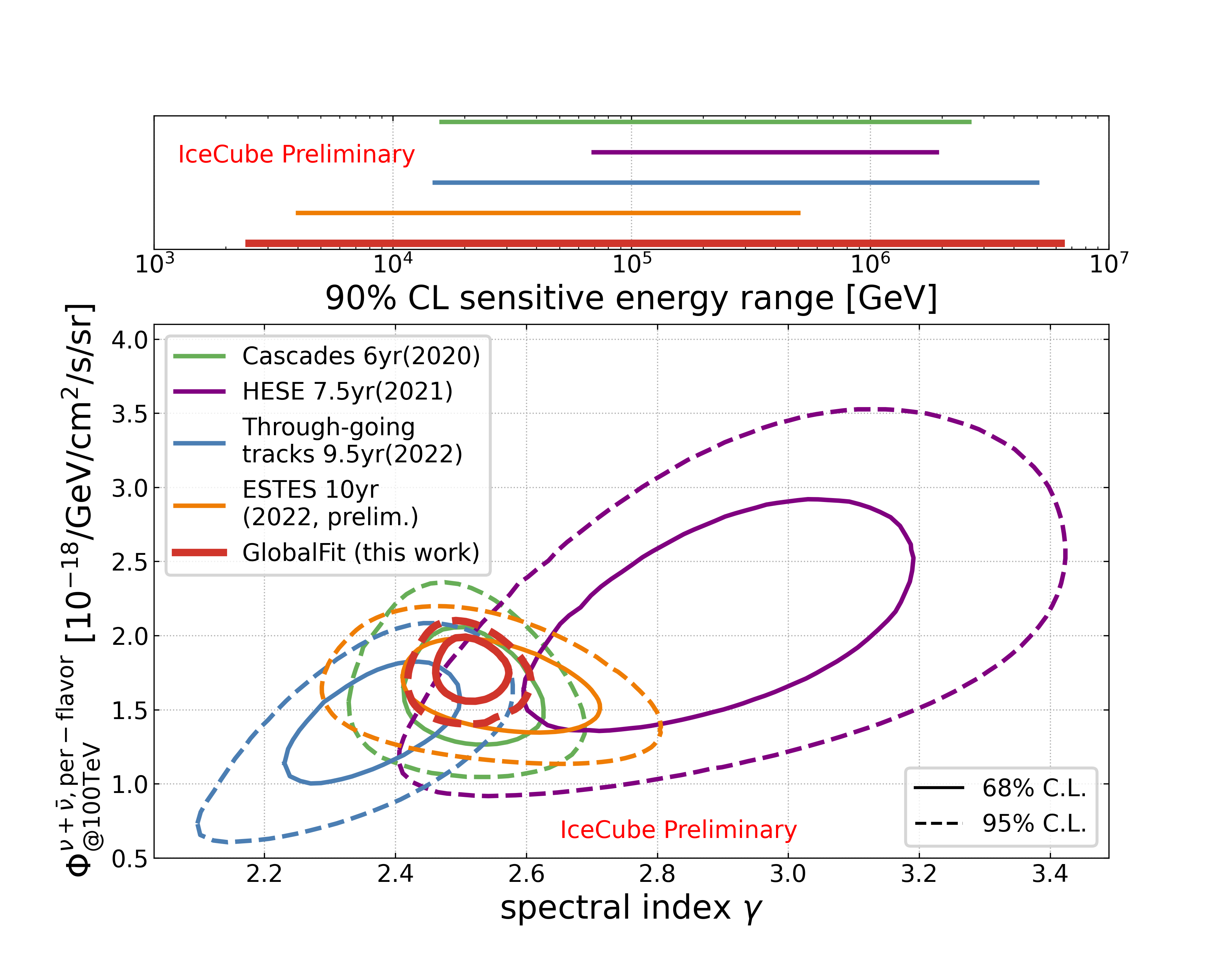
Figure 1: Result of the combined fit of tracks and cascades (in red) under the assumption of an astrophysical SPL neutrino flux. Previous results from measurements using single event channels are shown for comparison. Note that the sensitive neutrino energy ranges (as indicated in the upper panel) and neutrino flavor probed are different amongst the different samples.

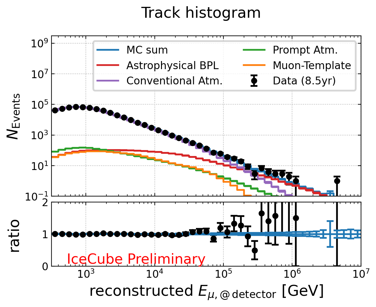
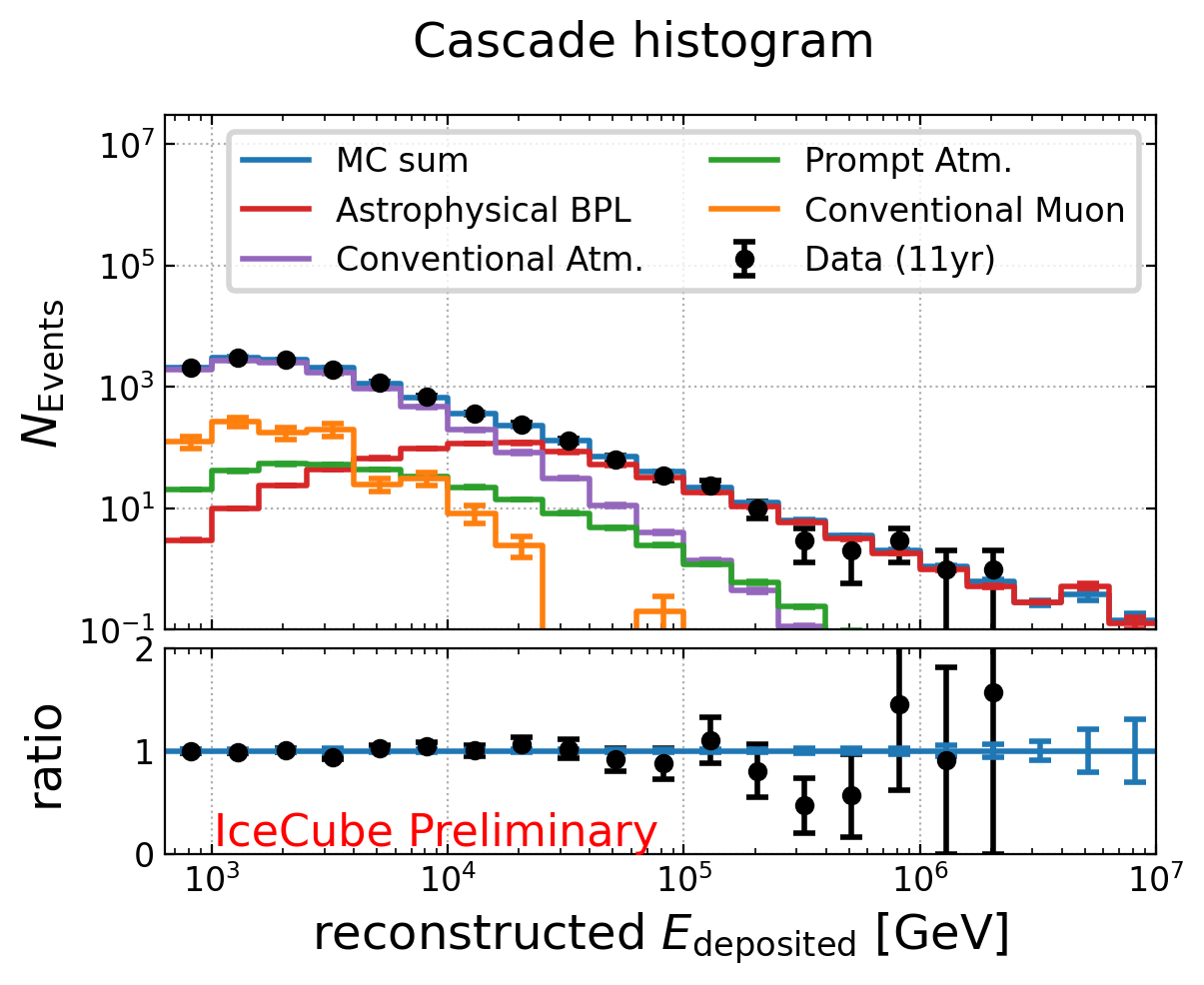
Figure 2: Best-fit spectra assuming a BPL astrophysical neutrino flux. Left: Reconstructed muon energy spectrum for all events in the tracks sample. Right: Reconstructed deposited energy spectrum for all events in the cascade sample.

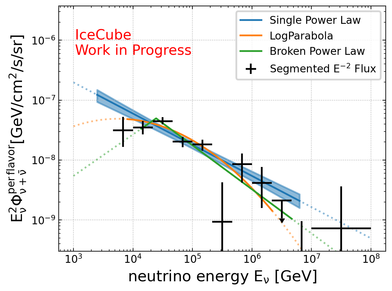
Figure 3: Result of the combined fit of tracks and cascades under different assumptions of the astrophysical neutrino flux. Solid lines represent the sensitive energy ranges of the corresponding astrophysical flux models. The uncertainty band shown in blue represents the 68% CL uncertainties on the SPL fit. The segmented flux fit uncertainties are obtained by profiling single-segment normalizations over all other parameters in the fit.

5 Conclusion and Outlook

For the first time, we perform a fit of two independent data samples of IceCube’s high-energy neutrino data using a consistent treatment of nuisance parameters. We find good agreement between the data and our model, with some deviations at the highest energies. We see indications for deviations from a SPL with hardening at lower energies and softening at higher energies, in agreement with what has been reported before using the tracks and cascades samples going into our combined fit. This opens up possibilities for deepening our understanding of the high-energy neutrino flux. The toolkit compiled for this work will be expanded with more event selections in the future for even better constraints on the astrophysical neutrino flux properties.

Full Author List: IceCube Collaboration

R. Abbasi¹⁷, M. Ackermann⁶³, J. Adams¹⁸, S. K. Agarwalla^40, 64, J. A. Aguilar¹², M. Ahlers²², J.M. Alameddine²³, N. M. Amin⁴⁴, K. Andeen⁴², G. Anton²⁶, C. Argüelles¹⁴, Y. Ashida⁵³, S. Athanasiadou⁶³, S. N. Axani⁴⁴, X. Bai⁵⁰, A. Balagopal V.⁴⁰, M. Baricevic⁴⁰, S. W. Barwick³⁰, V. Basu⁴⁰, R. Bay⁸, J. J. Beatty^20, 21, J. Becker Tjus^11, 65, J. Beise⁶¹, C. Bellenghi²⁷, C. Benning¹, S. BenZvi⁵², D. Berley¹⁹, E. Bernardini⁴⁸, D. Z. Besson³⁶, E. Blaufuss¹⁹, S. Blot⁶³, F. Bontempo³¹, J. Y. Book¹⁴, C. Boscolo Meneguolo⁴⁸, S. Böser⁴¹, O. Botner⁶¹, J. Böttcher¹, E. Bourbeau²², J. Braun⁴⁰, B. Brinson⁶, J. Brostean-Kaiser⁶³, R. T. Burley², R. S. Busse⁴³, D. Butterfield⁴⁰, M. A. Campana⁴⁹, K. Carloni¹⁴, E. G. Carnie-Bronca², S. Chattopadhyay^40, 64, N. Chau¹², C. Chen⁶, Z. Chen⁵⁵, D. Chirkin⁴⁰, S. Choi⁵⁶, B. A. Clark¹⁹, L. Classen⁴³, A. Coleman⁶¹, G. H. Collin¹⁵, A. Connolly^20, 21, J. M. Conrad¹⁵, P. Coppin¹³, P. Correa¹³, D. F. Cowen^59, 60, P. Dave⁶, C. De Clercq¹³, J. J. DeLaunay⁵⁸, D. Delgado¹⁴, S. Deng¹, K. Deoskar⁵⁴, A. Desai⁴⁰, P. Desiati⁴⁰, K. D. de Vries¹³, G. de Wasseige³⁷, T. DeYoung²⁴, A. Diaz¹⁵, J. C. Díaz-Vélez⁴⁰, M. Dittmer⁴³, A. Domi²⁶, H. Dujmovic⁴⁰, M. A. DuVernois⁴⁰, T. Ehrhardt⁴¹, P. Eller²⁷, E. Ellinger⁶², S. El Mentawi¹, D. Elsässer²³, R. Engel^31, 32, H. Erpenbeck⁴⁰, J. Evans¹⁹, P. A. Evenson⁴⁴, K. L. Fan¹⁹, K. Fang⁴⁰, K. Farrag¹⁶, A. R. Fazely⁷, A. Fedynitch⁵⁷, N. Feigl¹⁰, S. Fiedlschuster²⁶, C. Finley⁵⁴, L. Fischer⁶³, D. Fox⁵⁹, A. Franckowiak¹¹, A. Fritz⁴¹, P. Fürst¹, J. Gallagher³⁹, E. Ganster¹, A. Garcia¹⁴, L. Gerhardt⁹, A. Ghadimi⁵⁸, C. Glaser⁶¹, T. Glauch²⁷, T. Glüsenkamp^26, 61, N. Goehlke³², J. G. Gonzalez⁴⁴, S. Goswami⁵⁸, D. Grant²⁴, S. J. Gray¹⁹, O. Gries¹, S. Griffin⁴⁰, S. Griswold⁵², K. M. Groth²², C. Günther¹, P. Gutjahr²³, C. Haack²⁶, A. Hallgren⁶¹, R. Halliday²⁴, L. Halve¹, F. Halzen⁴⁰, H. Hamdaoui⁵⁵, M. Ha Minh²⁷, K. Hanson⁴⁰, J. Hardin¹⁵, A. A. Harnisch²⁴, P. Hatch³³, A. Haungs³¹, K. Helbing⁶², J. Hellrung¹¹, F. Henningsen²⁷, L. Heuermann¹, N. Heyer⁶¹, S. Hickford⁶², A. Hidvegi⁵⁴, C. Hill¹⁶, G. C. Hill², K. D. Hoffman¹⁹, S. Hori⁴⁰, K. Hoshina^40, 66, W. Hou³¹, T. Huber³¹, K. Hultqvist⁵⁴, M. Hünnefeld²³, R. Hussain⁴⁰, K. Hymon²³, S. In⁵⁶, A. Ishihara¹⁶, M. Jacquart⁴⁰, O. Janik¹, M. Jansson⁵⁴, G. S. Japaridze⁵, M. Jeong⁵⁶, M. Jin¹⁴, B. J. P. Jones⁴, D. Kang³¹, W. Kang⁵⁶, X. Kang⁴⁹, A. Kappes⁴³, D. Kappesser⁴¹, L. Kardum²³, T. Karg⁶³, M. Karl²⁷, A. Karle⁴⁰, U. Katz²⁶, M. Kauer⁴⁰, J. L. Kelley⁴⁰, A. Khatee Zathul⁴⁰, A. Kheirandish^34, 35, J. Kiryluk⁵⁵, S. R. Klein^8, 9, A. Kochocki²⁴, R. Koirala⁴⁴, H. Kolanoski¹⁰, T. Kontrimas²⁷, L. Köpke⁴¹, C. Kopper²⁶, D. J. Koskinen²², P. Koundal³¹, M. Kovacevich⁴⁹, M. Kowalski^10, 63, T. Kozynets²², J. Krishnamoorthi^40, 64, K. Kruiswijk³⁷, E. Krupczak²⁴, A. Kumar⁶³, E. Kun¹¹, N. Kurahashi⁴⁹, N. Lad⁶³, C. Lagunas Gualda⁶³, M. Lamoureux³⁷, M. J. Larson¹⁹, S. Latseva¹, F. Lauber⁶², J. P. Lazar^14, 40, J. W. Lee⁵⁶, K. Leonard DeHolton⁶⁰, A. Leszczyńska⁴⁴, M. Lincetto¹¹, Q. R. Liu⁴⁰, M. Liubarska²⁵, E. Lohfink⁴¹, C. Love⁴⁹, C. J. Lozano Mariscal⁴³, L. Lu⁴⁰, F. Lucarelli²⁸, W. Luszczak^20, 21, Y. Lyu^8, 9, J. Madsen⁴⁰, K. B. M. Mahn²⁴, Y. Makino⁴⁰, E. Manao²⁷, S. Mancina^40, 48, W. Marie Sainte⁴⁰, I. C. Mariş¹², S. Marka⁴⁶, Z. Marka⁴⁶, M. Marsee⁵⁸, I. Martinez-Soler¹⁴, R. Maruyama⁴⁵, F. Mayhew²⁴, T. McElroy²⁵, F. McNally³⁸, J. V. Mead²², K. Meagher⁴⁰, S. Mechbal⁶³, A. Medina²¹, M. Meier¹⁶, Y. Merckx¹³, L. Merten¹¹, J. Micallef²⁴, J. Mitchell⁷, T. Montaruli²⁸, R. W. Moore²⁵, Y. Morii¹⁶, R. Morse⁴⁰, M. Moulai⁴⁰, T. Mukherjee³¹, R. Naab⁶³, R. Nagai¹⁶, M. Nakos⁴⁰, U. Naumann⁶², J. Necker⁶³, A. Negi⁴, M. Neumann⁴³, H. Niederhausen²⁴, M. U. Nisa²⁴, A. Noell¹, A. Novikov⁴⁴, S. C. Nowicki²⁴, A. Obertacke Pollmann¹⁶, V. O’Dell⁴⁰, M. Oehler³¹, B. Oeyen²⁹, A. Olivas¹⁹, R. Ørsøe²⁷, J. Osborn⁴⁰, E. O’Sullivan⁶¹, H. Pandya⁴⁴, N. Park³³, G. K. Parker⁴, E. N. Paudel⁴⁴, L. Paul^42, 50, C. Pérez de los Heros⁶¹, J. Peterson⁴⁰, S. Philippen¹, A. Pizzuto⁴⁰, M. Plum⁵⁰, A. Pontén⁶¹, Y. Popovych⁴¹, M. Prado Rodriguez⁴⁰, B. Pries²⁴, R. Procter-Murphy¹⁹, G. T. Przybylski⁹, C. Raab³⁷, J. Rack-Helleis⁴¹, K. Rawlins³, Z. Rechav⁴⁰, A. Rehman⁴⁴, P. Reichherzer¹¹, G. Renzi¹², E. Resconi²⁷, S. Reusch⁶³, W. Rhode²³, B. Riedel⁴⁰, A. Rifaie¹, E. J. Roberts², S. Robertson^8, 9, S. Rodan⁵⁶, G. Roellinghoff⁵⁶, M. Rongen²⁶, C. Rott^53, 56, T. Ruhe²³, L. Ruohan²⁷, D. Ryckbosch²⁹, I. Safa^14, 40, J. Saffer³², D. Salazar-Gallegos²⁴, P. Sampathkumar³¹, S. E. Sanchez Herrera²⁴, A. Sandrock⁶², M. Santander⁵⁸, S. Sarkar²⁵, S. Sarkar⁴⁷, J. Savelberg¹, P. Savina⁴⁰, M. Schaufel¹, H. Schieler³¹, S. Schindler²⁶, L. Schlickmann¹, B. Schlüter⁴³, F. Schlüter¹², N. Schmeisser⁶², T. Schmidt¹⁹, J. Schneider²⁶, F. G. Schröder^31, 44, L. Schumacher²⁶, G. Schwefer¹, S. Sclafani¹⁹, D. Seckel⁴⁴, M. Seikh³⁶, S. Seunarine⁵¹, R. Shah⁴⁹, A. Sharma⁶¹, S. Shefali³², N. Shimizu¹⁶, M. Silva⁴⁰, B. Skrzypek¹⁴, B. Smithers⁴, R. Snihur⁴⁰, J. Soedingrekso²³, A. Søgaard²², D. Soldin³², P. Soldin¹, G. Sommani¹¹, C. Spannfellner²⁷, G. M. Spiczak⁵¹, C. Spiering⁶³, M. Stamatikos²¹, T. Stanev⁴⁴, T. Stezelberger⁹, T. Stürwald⁶², T. Stuttard²², G. W. Sullivan¹⁹, I. Taboada⁶, S. Ter-Antonyan⁷, M. Thiesmeyer¹, W. G. Thompson¹⁴, J. Thwaites⁴⁰, S. Tilav⁴⁴, K. Tollefson²⁴, C. Tönnis⁵⁶, S. Toscano¹², D. Tosi⁴⁰, A. Trettin⁶³, C. F. Tung⁶, R. Turcotte³¹, J. P. Twagirayezu²⁴, B. Ty⁴⁰, M. A. Unland Elorrieta⁴³, A. K. Upadhyay^40, 64, K. Upshaw⁷, N. Valtonen-Mattila⁶¹, J. Vandenbroucke⁴⁰, N. van Eijndhoven¹³, D. Vannerom¹⁵, J. van Santen⁶³, J. Vara⁴³, J. Veitch-Michaelis⁴⁰, M. Venugopal³¹, M. Vereecken³⁷, S. Verpoest⁴⁴, D. Veske⁴⁶, A. Vijai¹⁹, C. Walck⁵⁴, C. Weaver²⁴, P. Weigel¹⁵, A. Weindl³¹, J. Weldert⁶⁰, C. Wendt⁴⁰, J. Werthebach²³, M. Weyrauch³¹, N. Whitehorn²⁴, C. H. Wiebusch¹, N. Willey²⁴, D. R. Williams⁵⁸, L. Witthaus²³, A. Wolf¹, M. Wolf²⁷, G. Wrede²⁶, X. W. Xu⁷, J. P. Yanez²⁵, E. Yildizci⁴⁰, S. Yoshida¹⁶, R. Young³⁶, F. Yu¹⁴, S. Yu²⁴, T. Yuan⁴⁰, Z. Zhang⁵⁵, P. Zhelnin¹⁴, M. Zimmerman<sup>40

1</sup> III. Physikalisches Institut, RWTH Aachen University, D-52056 Aachen, Germany
² Department of Physics, University of Adelaide, Adelaide, 5005, Australia
³ Dept. of Physics and Astronomy, University of Alaska Anchorage, 3211 Providence Dr., Anchorage, AK 99508, USA
⁴ Dept. of Physics, University of Texas at Arlington, 502 Yates St., Science Hall Rm 108, Box 19059, Arlington, TX 76019, USA
⁵ CTSPS, Clark-Atlanta University, Atlanta, GA 30314, USA
⁶ School of Physics and Center for Relativistic Astrophysics, Georgia Institute of Technology, Atlanta, GA 30332, USA
⁷ Dept. of Physics, Southern University, Baton Rouge, LA 70813, USA
⁸ Dept. of Physics, University of California, Berkeley, CA 94720, USA
⁹ Lawrence Berkeley National Laboratory, Berkeley, CA 94720, USA
¹⁰ Institut für Physik, Humboldt-Universität zu Berlin, D-12489 Berlin, Germany
¹¹ Fakultät für Physik & Astronomie, Ruhr-Universität Bochum, D-44780 Bochum, Germany
¹² Université Libre de Bruxelles, Science Faculty CP230, B-1050 Brussels, Belgium
¹³ Vrije Universiteit Brussel (VUB), Dienst ELEM, B-1050 Brussels, Belgium
¹⁴ Department of Physics and Laboratory for Particle Physics and Cosmology, Harvard University, Cambridge, MA 02138, USA
¹⁵ Dept. of Physics, Massachusetts Institute of Technology, Cambridge, MA 02139, USA
¹⁶ Dept. of Physics and The International Center for Hadron Astrophysics, Chiba University, Chiba 263-8522, Japan
¹⁷ Department of Physics, Loyola University Chicago, Chicago, IL 60660, USA
¹⁸ Dept. of Physics and Astronomy, University of Canterbury, Private Bag 4800, Christchurch, New Zealand
¹⁹ Dept. of Physics, University of Maryland, College Park, MD 20742, USA
²⁰ Dept. of Astronomy, Ohio State University, Columbus, OH 43210, USA
²¹ Dept. of Physics and Center for Cosmology and Astro-Particle Physics, Ohio State University, Columbus, OH 43210, USA
²² Niels Bohr Institute, University of Copenhagen, DK-2100 Copenhagen, Denmark
²³ Dept. of Physics, TU Dortmund University, D-44221 Dortmund, Germany
²⁴ Dept. of Physics and Astronomy, Michigan State University, East Lansing, MI 48824, USA
²⁵ Dept. of Physics, University of Alberta, Edmonton, Alberta, Canada T6G 2E1
²⁶ Erlangen Centre for Astroparticle Physics, Friedrich-Alexander-Universität Erlangen-Nürnberg, D-91058 Erlangen, Germany
²⁷ Technical University of Munich, TUM School of Natural Sciences, Department of Physics, D-85748 Garching bei München, Germany
²⁸ Département de physique nucléaire et corpusculaire, Université de Genève, CH-1211 Genève, Switzerland
²⁹ Dept. of Physics and Astronomy, University of Gent, B-9000 Gent, Belgium
³⁰ Dept. of Physics and Astronomy, University of California, Irvine, CA 92697, USA
³¹ Karlsruhe Institute of Technology, Institute for Astroparticle Physics, D-76021 Karlsruhe, Germany
³² Karlsruhe Institute of Technology, Institute of Experimental Particle Physics, D-76021 Karlsruhe, Germany
³³ Dept. of Physics, Engineering Physics, and Astronomy, Queen’s University, Kingston, ON K7L 3N6, Canada
³⁴ Department of Physics & Astronomy, University of Nevada, Las Vegas, NV, 89154, USA
³⁵ Nevada Center for Astrophysics, University of Nevada, Las Vegas, NV 89154, USA
³⁶ Dept. of Physics and Astronomy, University of Kansas, Lawrence, KS 66045, USA
³⁷ Centre for Cosmology, Particle Physics and Phenomenology - CP3, Université catholique de Louvain, Louvain-la-Neuve, Belgium
³⁸ Department of Physics, Mercer University, Macon, GA 31207-0001, USA
³⁹ Dept. of Astronomy, University of Wisconsin–Madison, Madison, WI 53706, USA
⁴⁰ Dept. of Physics and Wisconsin IceCube Particle Astrophysics Center, University of Wisconsin–Madison, Madison, WI 53706, USA
⁴¹ Institute of Physics, University of Mainz, Staudinger Weg 7, D-55099 Mainz, Germany
⁴² Department of Physics, Marquette University, Milwaukee, WI, 53201, USA
⁴³ Institut für Kernphysik, Westfälische Wilhelms-Universität Münster, D-48149 Münster, Germany
⁴⁴ Bartol Research Institute and Dept. of Physics and Astronomy, University of Delaware, Newark, DE 19716, USA
⁴⁵ Dept. of Physics, Yale University, New Haven, CT 06520, USA
⁴⁶ Columbia Astrophysics and Nevis Laboratories, Columbia University, New York, NY 10027, USA
⁴⁷ Dept. of Physics, University of Oxford, Parks Road, Oxford OX1 3PU, United Kingdom
⁴⁸ Dipartimento di Fisica e Astronomia Galileo Galilei, Università Degli Studi di Padova, 35122 Padova PD, Italy
⁴⁹ Dept. of Physics, Drexel University, 3141 Chestnut Street, Philadelphia, PA 19104, USA
⁵⁰ Physics Department, South Dakota School of Mines and Technology, Rapid City, SD 57701, USA
⁵¹ Dept. of Physics, University of Wisconsin, River Falls, WI 54022, USA
⁵² Dept. of Physics and Astronomy, University of Rochester, Rochester, NY 14627, USA
⁵³ Department of Physics and Astronomy, University of Utah, Salt Lake City, UT 84112, USA
⁵⁴ Oskar Klein Centre and Dept. of Physics, Stockholm University, SE-10691 Stockholm, Sweden
⁵⁵ Dept. of Physics and Astronomy, Stony Brook University, Stony Brook, NY 11794-3800, USA
⁵⁶ Dept. of Physics, Sungkyunkwan University, Suwon 16419, Korea
⁵⁷ Institute of Physics, Academia Sinica, Taipei, 11529, Taiwan
⁵⁸ Dept. of Physics and Astronomy, University of Alabama, Tuscaloosa, AL 35487, USA
⁵⁹ Dept. of Astronomy and Astrophysics, Pennsylvania State University, University Park, PA 16802, USA
⁶⁰ Dept. of Physics, Pennsylvania State University, University Park, PA 16802, USA
⁶¹ Dept. of Physics and Astronomy, Uppsala University, Box 516, S-75120 Uppsala, Sweden
⁶² Dept. of Physics, University of Wuppertal, D-42119 Wuppertal, Germany
⁶³ Deutsches Elektronen-Synchrotron DESY, Platanenallee 6, 15738 Zeuthen, Germany
⁶⁴ Institute of Physics, Sachivalaya Marg, Sainik School Post, Bhubaneswar 751005, India
⁶⁵ Department of Space, Earth and Environment, Chalmers University of Technology, 412 96 Gothenburg, Sweden
⁶⁶ Earthquake Research Institute, University of Tokyo, Bunkyo, Tokyo 113-0032, Japan

Acknowledgements

The authors gratefully acknowledge the support from the following agencies and institutions: USA – U.S. National Science Foundation-Office of Polar Programs, U.S. National Science Foundation-Physics Division, U.S. National Science Foundation-EPSCoR, Wisconsin Alumni Research Foundation, Center for High Throughput Computing (CHTC) at the University of Wisconsin–Madison, Open Science Grid (OSG), Advanced Cyberinfrastructure Coordination Ecosystem: Services & Support (ACCESS), Frontera computing project at the Texas Advanced Computing Center, U.S. Department of Energy-National Energy Research Scientific Computing Center, Particle astrophysics research computing center at the University of Maryland, Institute for Cyber-Enabled Research at Michigan State University, and Astroparticle physics computational facility at Marquette University; Belgium – Funds for Scientific Research (FRS-FNRS and FWO), FWO Odysseus and Big Science programmes, and Belgian Federal Science Policy Office (Belspo); Germany – Bundesministerium für Bildung und Forschung (BMBF), Deutsche Forschungsgemeinschaft (DFG), Helmholtz Alliance for Astroparticle Physics (HAP), Initiative and Networking Fund of the Helmholtz Association, Deutsches Elektronen Synchrotron (DESY), and High Performance Computing cluster of the RWTH Aachen; Sweden – Swedish Research Council, Swedish Polar Research Secretariat, Swedish National Infrastructure for Computing (SNIC), and Knut and Alice Wallenberg Foundation; European Union – EGI Advanced Computing for research; Australia – Australian Research Council; Canada – Natural Sciences and Engineering Research Council of Canada, Calcul Québec, Compute Ontario, Canada Foundation for Innovation, WestGrid, and Compute Canada; Denmark – Villum Fonden, Carlsberg Foundation, and European Commission; New Zealand – Marsden Fund; Japan – Japan Society for Promotion of Science (JSPS) and Institute for Global Prominent Research (IGPR) of Chiba University; Korea – National Research Foundation of Korea (NRF); Switzerland – Swiss National Science Foundation (SNSF); United Kingdom – Department of Physics, University of Oxford.

References

- [1] IceCube Collaboration, M. G. Aartsen et al. Science 342 (2013) 1242856.
- [2] IceCube Collaboration, R. Abbasi et al. Phys. Rev. D 104 (Jul, 2021) 022002.
- [3] IceCube Collaboration, R. Abbasi et al. Astrophys. J. 928 no. 1, (2022) 50.
- [4] IceCube Collaboration, M. G. Aartsen et al. Phys. Rev. Lett. 125 no. 12, (2020) 121104.
- [5] IceCube Collaboration, M. G. Aartsen et al. Astrophys. J. 809 no. 1, (2015) 98.
- [6] E. Ganster, “ 2022, https://indico.cern.ch/event/1082486/contributions/4878592/.”.
- [7] R. Naab, “ 2022, https://indico.cern.ch/event/1082486/contributions/4878588/.”.
- [8] C. A. Argüelles et al. JCAP 07 (2018) 047.
- [9] M. Aartsen et al. Journal of Instrumentation 15 no. 06, (Jun, 2020) P06032.
- [10] IceCube Collaboration, T. Yuan et al. Nucl. Instrum. Meth. A (2023) 168440.
- [11] IceCube Collaboration, M. G. Aartsen et al. JCAP 10 (2019) 048.
- [12] IceCube Collaboration, R. Abbasi et al. PoS ICRC2021 (2021) 1129.
- [13] A. Cooper-Sarkar et al. JHEP 08 (2011) 042.
- [14] J. H. Koehne et al. Comput. Phys. Commun. 184 (2013) 2070–2090.
- [15] A. Fedynitch et al. EPJ Web of Conferences 99 (2015) 08001.
- [16] G. D. Barr et al. Phys. Rev. D 74 no. 9, (Nov., 2006) 094009.
- [17] C. A. Argüelles et al. JHEP 06 (2019) 030.
- [18] B. T. Willard et al., “Aesara.” Aesara developers, 2023. https://github.com/aesara-devs/aesara.
- [19] IceCube Collaboration, M. G. Aartsen et al. Phys. Rev. D 91 no. 2, (2015) 022001.
- [20] IceCube Collaboration PoS ICRC2023 (these proceedings) 1068.
- [21] IceCube Collaboration PoS ICRC2023 (these proceedings) 1008.
- [22] R. Abbasi et al. Science 380 (7, 2023) 6652.
- [23] R. Abbasi et al. The Cryosphere Discussions 2022 (2022) 1–48.