Abstract

Pauli channels are fundamental in the context of quantum computing as they model the simplest kind of noise in quantum devices. We propose a quantum algorithm for simulating Pauli channels and extend it to encompass Pauli dynamical maps (parametrized Pauli channels). A parametrized quantum circuit is employed to accommodate for dynamical maps. We also establish the mathematical conditions for an $N$-qubit transformation to be achievable using a parametrized circuit where only one single-qubit operation depends on the parameter. The implementation of the proposed circuit is demonstrated using IBM’s quantum computers for the case of one qubit, and the fidelity of this implementation is reported.

1 Introduction

Since their inception, quantum computers were proposed as powerful tools for the simulation of quantum systems [1]. Being open quantum systems of fundamental [2, 3] and practical [4] interest, there has been efforts towards the simulation of the evolution of open quantum systems [5, 6, 7] and specifically for quantum channels [8, 9, 10].

Such systems have been simulated because of their many applications, such as studying the emergence of multipartite entanglement [11, 12], studying dissipative processes [13] and modeling non-Markovian dynamics [14]. Among quantum systems, the simplest case is that of a qubit [15], and withing them, the simplest class of channels that produce decoherence are Pauli channels [16, 17, 18]. Indeed, they serve as effective models for the noise affecting quantum devices [19].

To represent the algorithms implemented in quantum computers, either to simulate a physical system or for some other purpose, one often uses a quantum circuit [15]. In this work, we shall also work with parametrized quantum circuits, that is, quantum circuits in which some of the operations depend on variable parameters [20]. These circuits play an important part in applications such as quantum machine learning [21] and describing general quantum transformations dependent on parameters. Substantial research has been devoted to enhancing the efficiency of these circuits [22].

We start by providing the definition of quantum channels, the general framework used here, and multi-qubit Pauli channels in section 2. Our first objective is to present a quantum algorithm capable of simulating Pauli channels on quantum computers; we do this in section 3, where we also demonstrate its implementation using IBM’s quantum computers for the particular case of single-qubit Pauli channels. Expanding beyond discrete Pauli channels, we introduce the concept of Pauli dynamical maps, defined as a continuous parametrization of multi-qubit Pauli channels. Therefore, in section 4 we shift our focus to study parametrized quantum channels, aiming to adapt the algorithm developed for channels to dynamical maps. Furthermore, we contribute to the body of work related to parametrized quantum circuits by establishing a theorem, which sets the mathematical conditions for the transformations that can be done using a parametrized circuit with the condition that only a controlled single-qubit rotation in the circuit may depend on the parameter. Finally, in section 5, we conclude about the Pauli dynamical maps that fulfill the conditions of theorem 2.

2 Pauli channels and dynamical maps

In this section we introduce the concept of quantum channels, focusing on a specific type called Pauli channels. Furthermore, we define Pauli dynamical maps, which are curves of Pauli channels parametrized by a variable.

2.1 Quantum channels

In quantum mechanics, a closed system’s state is represented by a vector in a Hilbert space $\mathcal{H}$. The state’s evolution is unitary and given by Schrodinger’s equation [23]. However, in real-world situations, quantum systems are usually open, which means that they interact with their environment [4]. For instance, the system’s state may become entangled with the environment, leading to a loss of information about the system’s state over time.

To describe open systems, instead of state vectors, we use matrices $\rho$ that act on $\mathcal{H}$. These matrices are called density matrices, and they include information about the system’s interaction with its environment. For a density matrix $\rho$ to be physically valid, it must satisfy two conditions: $\operatorname{tr}(\rho)=1$ and it must be positive semi-definite, which is denoted as $\rho\geq 0$ [15].

Knowing this, we can now define quantum channels. Quantum channels are operators $\mathcal{E}$ that can describe the evolution of open quantum systems, such that $\rho\rightarrow\mathcal{E}(\rho)$. Quantum channels are the most general linear operations that a quantum system can undergo independently of its past [24, 25]. These channels are constructed based on three fundamental properties: linearity, trace preservation, and complete positivity.

Linearity ensures that a quantum channel $\mathcal{E}$ maps any ensemble of density matrices into the corresponding ensemble of their evolution. The trace preserving property is given by $\operatorname{tr}(\mathcal{E}[\rho])=\operatorname{tr}(\rho)=1$ and guarantees that the quantum channel does not change the condition that $\operatorname{tr}(\rho)=1$. Finally, the channel should also preserve the condition $\rho\geq 0$, and a map that does this is called a positive map. However, positivity of $\mathcal{E}$ is not enough, and we actually require the more restrictive condition of complete positivity. Complete positivity means that $\mathcal{E}\otimes\mathbb{I}_{n}$ is positive for any positive integer $n$ (where $\mathbb{I}_{n}$ is the $n\times n$ identity matrix). This ensures that even if the principal system is entangled with another system, applying $\mathcal{E}$ to the principal system while doing nothing to the other one still results in a positive semidefinite state for the principal system [15].

Given a quantum channel $\mathcal{E}$, the condition of trace preservation is straightforward to verify but complete positivity is not as simple. To test complete positivity of a quantum channel, Jamiołkowski and Choi [26, 27] developed a simple algorithm that exploits the isomorphism between a channel $\mathcal{E}$ and the state $\mathcal{D}=(\mathbb{I}\otimes\mathcal{E})[|\Omega\rangle\langle\Omega|]$, where $|\Omega\rangle=1/\text{dim}(\mathcal{H})\sum_{i}^{\text{dim}(\mathcal{H})}|i\rangle|i\rangle$ is a maximally entangled state between the original system and an ancilla. Remarkably, the map $\mathcal{E}$ is completely positive if and only if $\mathcal{D}$ (also known as the Choi or dynamical matrix of $\mathcal{E}$) is positive semidefinite.

2.2 Pauli channels

We have discussed the main features of quantum channels and now we turn our attention to a specific type of channels for $N$-qubit systems called Pauli channels. First we will define these channels for single-qubit systems, whose most general density matrix can be written as [15]:

$$\rho=\dfrac{1}{2}\sum_{\alpha=0}^{3}r_{\alpha}\sigma_{\alpha},$$ (1)

with $\sigma_{0}=\mathbb{I}$, and $\sigma_{1,2,3}$ the usual Pauli matrices. The condition $\operatorname{tr}(\rho)=1$ requires that $r_{0}=1$ while $\rho\geq 0$ implies that the remaining $r_{1,2,3}$ form a vector $\vec{r}=(r_{1},r_{2},r_{3})$ inside a unit sphere known as the Bloch sphere [28]. That is, every possible density matrix for a one-qubit system is uniquely associated with a point in a unit sphere.

Given a one-qubit system described by $\rho$, a Pauli channel is defined as an operation that with probability $k_{\gamma}$ applies the Pauli matrix $\sigma_{\gamma}$ to the system, for $\gamma=0,1,2,3$ [16]. Mathematically, the Pauli channel is written in the following way:

$$\mathcal{E}(\rho)=\sum_{\gamma=0}^{3}k_{\gamma}\sigma_{\gamma}\rho\sigma_{\gamma},$$ (2)

where the probabilities $k_{\gamma}$ of applying $\sigma_{\gamma}$ are non-negative real numbers such that $\sum_{\gamma}k_{\gamma}=1$ (these conditions also ensure that the channel is trace preserving and completely positive).

Pauli channels are some of the most fundamental noise models in quantum information science [29]. Some notable examples of Pauli channels are the following:

• Bit Flip Channel: This is a channel that with probability $1-p$ leaves the qubit as it is and with probability $p$ applies the $\sigma_{1}$ matrix (which flips the basis states $|0\rangle$ and $|1\rangle$ of the qubit), and so it is given by:

  $$\mathcal{E}(\rho)=(1-p)\rho+p\sigma_{1}\rho\sigma_{1}.$$

  Analogous channels exist using $\sigma_{3}$ (called the bit flip channel, which has a probability $p$ of adding a relative phase $\pi$ to the state) or using $\sigma_{2}$ (called the phase flip channel, which has a probability $p$ of flipping the base states and also add a relative phase $\pi$).

• Depolarizing channel: This channel has a probability $1-p$ of doing nothing to the qubit and a probability $p$ of converting it into the maximally mixed state $\dfrac{1}{2}\mathbb{I}$ and it can be written as:

  $$\mathcal{E}(\rho)=(1-p)\rho+p\dfrac{1}{2}\mathbb{I}=\left(1-\dfrac{3p}{4}\right)\sigma+\dfrac{p}{4}\sigma_{1}\rho\sigma_{1}+\dfrac{p}{4}\sigma_{2}\rho\sigma_{2}+\dfrac{p}{4}\sigma_{3}\rho\sigma_{3}.$$ (3)

We can also see how an arbitrary Pauli channel acts on an arbitrary density matrix. To do it, we substitute Eq (1) in Eq (2):

$$\mathcal{E}(\rho)=\dfrac{1}{2}\sum_{\gamma,\alpha=0}^{3}k_{\gamma}r_{\alpha}\sigma_{\gamma}\sigma_{\alpha}\sigma_{\gamma}.$$ (4)

This can be simplified by using the following property of Pauli matrices:

$$\sigma_{\gamma}\sigma_{\alpha}\sigma_{\gamma}=A_{\alpha,\gamma}\sigma_{\alpha},\;\;\;\;\;\text{with}\;A_{\alpha,\gamma}=\begin{pmatrix}1&1&1&1\\ 1&1&-1&-1\\ 1&-1&1&-1\\ 1&-1&-1&1\end{pmatrix},$$ (5)

which leads to

$$\mathcal{E}(\rho)=\dfrac{1}{2}\sum_{\alpha}\left(\sum_{\gamma}A_{\alpha,\gamma}k_{\gamma}\right)r_{\alpha}\sigma_{\alpha}.$$ (6)

Eq (6) once again has the form of Eq (1) but with components $\left(\sum_{\gamma}A_{\alpha,\gamma}k_{\gamma}\right)r_{\alpha}$. This gives us another way of understanding Pauli channels as operations that take each component $r_{\alpha}$ of the density matrix and multiplies them by $\sum_{\gamma}A_{\alpha,\gamma}k_{\gamma}$, that is:

$$r_{\alpha}\xrightarrow[\text{Channel}]{\text{Pauli}}\tau_{\alpha}r_{\alpha},\;\;\tau_{\alpha}:=\sum_{\gamma}A_{\alpha,\gamma}k_{\gamma}.$$ (7)

Notice that $\tau_{0}=1$, which is a consequence of $\sum_{\gamma}k_{\gamma}=1$ and ensures that after the channel, the resulting density matrix still has trace one. Furthermore, reverting the definition of $\tau_{\alpha}$ by using that $A^{-1}=\dfrac{1}{4}A$, we get that $k_{\gamma}=\dfrac{1}{4}\sum_{\alpha}A_{\alpha,\gamma}\tau_{\alpha}$. Then, using that $k_{\gamma}\geq 0$ we get the following conditions on the multipliers $\tau_{\alpha}$:

$$1+\tau_{i}-\tau_{j}-\tau_{k}\geq 0,\;\;\;\text{for $i,j,k$ different numbers in $\{1,2,3\}$},$$ (8)

$$1+\tau_{1}+\tau_{2}+\tau_{3}\geq 0.$$ (9)

These conditions imply that $(\tau_{1},\tau_{2},\tau_{3})$ has to be inside a tetrahedron with vertices $(1,1,1),(1,-1,-1),(-1,1,-1)$ and $(-1,-1,1)$. Therefore, the $\tau_{1,2,3}$ are numbers between $-1$ and $1$, which means that the components $r_{\alpha}$ of the density matrix are always attenuated and possibly sign flipped.

Having defined the one qubit case, we can now generalize to $N$ qubits. In order to do it, we need to introduce the so-called Pauli strings, defined as

$$\sigma_{\vec{\alpha}}=\sigma_{\alpha_{1}}\otimes\sigma_{\alpha_{2}}\otimes\cdots\otimes\sigma_{\alpha_{N}},$$ (10)

where $\vec{\alpha}$ denotes a multi-index $(\alpha_{1},\cdots,\alpha_{N})$ and $\alpha_{i}\in\{0,1,2,3\}$. These operators form an orthogonal basis in the space of operators acting on $N$ qubits. Similarly to the single-qubit case, the density matrix $\rho$ of a system of $N$ qubits can be written using Pauli strings as:

$$\rho=\dfrac{1}{2^{N}}\sum_{\vec{\alpha}}r_{\vec{\alpha}}\sigma_{\vec{\alpha}}.$$ (11)

Then, just as before, we define a Pauli channel as a transformation that applies the operator $\sigma_{\vec{\gamma}}$ to $\rho$ with probability $k_{\vec{\gamma}}$ and is therefore described mathematically by:

$$\mathcal{E}(\rho)=\sum_{\vec{\gamma}}k_{\vec{\gamma}}\sigma_{\vec{\gamma}}\rho\sigma_{\vec{\gamma}},$$ (12)

where just as before, $k_{\vec{\gamma}}$ are non-negative real numbers such that $\sum_{\vec{\gamma}}k_{\vec{\gamma}}=1$.

As in the one qubit case, Pauli channels for $N$ qubits attenuate the components $r_{\vec{\alpha}}$ of the density matrix. This can be seen by substituting Eq (11) in Eq (12) and using the property of Eq (5):

$$\mathcal{E}(\rho) =\dfrac{1}{2^{N}}\sum_{\vec{\gamma},\vec{\alpha}}k_{\vec{\gamma}}r_{\vec{\alpha}}\sigma_{\vec{\gamma}}\sigma_{\vec{\alpha}}\sigma_{\vec{\gamma}}$$

$$=\dfrac{1}{2^{N}}\sum_{\vec{\alpha}}\left(\sum_{\vec{\gamma}}{(A^{\otimes^{N}})}_{\vec{\alpha},\vec{\gamma}}\;k_{\vec{\gamma}}\right)r_{\vec{\alpha}}\sigma_{\vec{\alpha}},$$

which means that applying the Pauli channel multiplies the components $r_{\vec{\alpha}}$ by $\tau_{\vec{\alpha}}:=\sum_{\vec{\gamma}}{(A^{\otimes^{N}})}_{\vec{\alpha},\vec{\gamma}}k_{\vec{\gamma}}$.

2.3 Pauli dynamical maps

As seen in the last section, Pauli channels and in general quantum channels are discrete maps that transform a density matrix $\rho$ into $\mathcal{E}(\rho)$. However, we could also define a continuous set of channels $\varepsilon_{p}$ with $p$ a real parameter.

For the special case of Pauli channels, we define a Pauli dynamical map as a continuous parametrized curve drawn inside the set of Pauli channels and starting at the identity channel. Therefore, a Pauli dynamical map can be written as

$$\mathcal{E}_{p}(\rho)=\sum_{\vec{\gamma}}k_{\vec{\gamma}}(p)\sigma_{\vec{\gamma}}\rho\sigma_{\vec{\gamma}},$$ (13)

where $p$ is a parameter in an interval $[a,b]$ and $\mathcal{E}_{p}$ is a Pauli channel for every $p$, with $\mathcal{E}_{a}$ being the identity channel.

3 Circuit for a Pauli channel

In this section we propose a quantum circuit that simulates $N$-qubit Pauli channels. Moreover, we implement the circuit for $N=1$ on a quantum computer and analyze the results using the diamond norm. We find that close to the depolarizing channel, the general circuit simulator can implement such channels with the highest fidelity.

3.1 Description of the circuit for a Pauli channel

To design the circuit that implements Eq (12), we construct a state that includes the probabilities $k_{\gamma}$ on the ancilla qubits and subsequently apply controlled Pauli operations on the main qubits. The circuit that does this is presented in Fig 1.

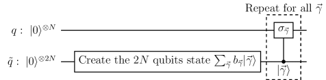
Figure 1: Circuit for an $N$-qubit Pauli channel. The circuit creates the state $\sum_{\vec{\gamma}}b_{\vec{\gamma}}|\vec{\gamma}\rangle$ on the $2N$ ancilla qubits denoted by $\tilde{q}$.

The first part of the circuit involves the creation of the state

$$\text{Ancilla state =}\sum_{\vec{\gamma}}b_{\vec{\gamma}}|\vec{\gamma}\rangle$$ (14)

on the ancilla qubits, where $b_{\vec{\gamma}}$ are numbers such that ${|b_{\vec{\gamma}}|}^{2}=k_{\vec{\gamma}}$ and the $2N$-qubit state $|\vec{\gamma}\rangle$ is defined as $|\gamma_{1}\rangle\cdots|\gamma_{N}\rangle$. When measured in the computational basis, the state given in Eq (14) collapses to $|\vec{\gamma}\rangle$ with a probability ${|b_{\vec{\gamma}}|}^{2}=k_{\vec{\gamma}}$. The circuit in Fig 1 uses this fact to apply $\sigma_{\vec{\gamma}}$ on the main qubits with a probability $k_{\vec{\gamma}}$ by using controlled operations conditioned on the state of the system being $|\vec{\gamma}\rangle$, just as the Pauli channel is supposed to do.

3.2 Simulation for one-qubit Pauli channels

For the particular case of a Pauli channel on one qubit, the circuit that simulates it can be constructed as in Fig 2, which is a special case of Fig 1 but with all details explicitly shown. In said figure, the ancilla state of Eq (14) can be taken to be $\sqrt{k_{0}}|00\rangle+\sqrt{k_{1}}|01\rangle+\sqrt{k_{2}}|10\rangle+\sqrt{k_{3}}|11\rangle$ and it is created on the ancilla qubits with the help of three rotations of angles defined by the following equations:

$$\cos\left(\dfrac{\theta_{0}}{2}\right) =\sqrt{k_{0}+k_{1}},$$

$$\tan\left(\dfrac{\theta_{1}+\theta_{2}}{2}\right) =\sqrt{k_{1}/k_{0}},$$ (15)

$$\tan\left(\dfrac{\theta_{2}-\theta_{1}}{2}\right) =\sqrt{k_{3}/k_{2}}.$$

Figure 2: One-qubit Pauli channel circuit. Circuit for a one-qubit Pauli channel, which is a particular case of Fig 1. Here we have two ancilla qubits and we use three rotations of angles given by Eq (3.2) to create the Ancilla State of of Eq (14) for the two ancilla qubits.

We took a sample of one-qubit Pauli channels and evaluated their implementation on IBM’s ibmq-lima quantum computer [30], as shown in Fig 3. For each of the channels sampled, we used quantum process tomography [30, 31] to obtain the operator $\xi_{I}$ corresponding to the implementation of the circuit in the quantum computer. Then, we compared $\xi_{I}$ with the theoretical operator $\xi_{T}$ of the Pauli channel we wanted to implement. To see how close the operators $\xi_{I}$ and $\xi_{T}$ are, we shall use the diamond distance [32], which is defined by

$$||\xi_{I}-\xi_{T}||_{\diamond}=\max_{\rho}||(\xi_{I}\otimes I)\rho-(\xi_{T}\otimes I)\rho||_{1},$$ (16)

with $I$ the identity map, $||\cdot||_{1}$ the trace norm and the maximization done over all density matrices $\rho$. The calculation of this norm is done using the semi-definite program from reference [33]. When the two channels are the same, the diamond distance has a value of $0$, while in the case that the channels are completely distinguishable, the distance reaches its maximum value of $2$ [34]. For the analysis done in Fig 3, we define a sort of “diamond fidelity” as:

$$f=1-\dfrac{1}{2}||\varepsilon_{I}-\varepsilon_{T}||_{\diamond},$$ (17)

which ranges from $0$, when the channels have a maximum distance, to $1$, when they are exactly equal.

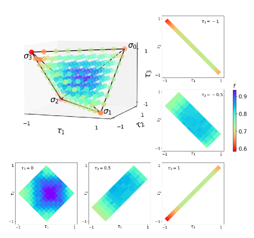
Figure 3: Results of the diamond fidelities as defined in Eq (17) for a sample of Pauli channels in the tetrahedron. Notice that channels close to the center of the tetrahedron have high fidelities, while those close to the borders do not. Moreover, we show the results for cuts of the tetrahedron at different values of $\tau_{3}$.

Finally, using the representation of Pauli channels in a tetrahedron as in Eq (8), we show in Fig 3 the diamond fidelity defined by Eq (17) for the channels analyzed. We can see that channels close to the completely depolarizing channel (that is close to the center of the tetrahedron) have a high $f$, while those close to unitary channels have much lower $f$. This is reasonable because quantum computers are prone to errors that depolarize qubits, which isn’t very problematic when trying to simulate depolarization but it is when simulating unitary processes. Moreover, the algorithm of Fig 2 is not optimal for unitary channels (that is, the channels corresponding to the vertices of the tetrahedron). These straightforward channels could be accomplished more efficiently by simply applying the corresponding Pauli operation directly. Nevertheless, due to its general design to accommodate any Pauli channel, the algorithm employs numerous quantum gates even in such scenarios.

4 One parameter circuits

Just as Pauli channels, Pauli dynamical maps can be implemented using the circuit of Fig 1. However, there is one difference: the state to be created on the ancilla qubits now depends on a parameter $p$, and it is represented by the expression:

$$\sum_{\vec{\gamma}}b_{\vec{\gamma}}(p)|\vec{\gamma}\rangle.$$ (18)

Thus, we temporarily shift our focus from Pauli channels and dynamical maps to the general problem of creating a circuit to generate a curve of states like the one described in Eq (18).

In general, producing this curve of states for $N$ qubits will require many rotations parametrized by $p$, such as the three rotations used for the ancilla qubits in Fig 2. However, it would be preferable to achieve the same effect using only one parametrized rotation. This would allow us to interpret said rotation as a knob that smoothly traverses the curve of states. Consequently, we are faced with the question of which curves of states, such as the one described in Eq (18), can be produced using just a single parametrized rotation. To clarify this, we provide the following definition for a circuit with one parametrized rotation.

Definition 1

1-Parameter Rotation Circuit: A 1-Parameter Rotation (1PR) circuit is a parametrized quantum circuit that includes only one gate dependent on a parameter $p$. Moreover, the parametrized gate is a one-qubit rotation about any axis, whether controlled or not.

Based on this definition, we aim to determine which curves of states can be generated using 1PR circuits. To accomplish this, we begin by proving that all 1PR circuits have the form depicted in Fig 4, where the parametrized rotation is around $\sigma_{3}$ and is applied to the last qubit.

Figure 4: General form of a 1PR circuit. Any 1PR circuit can be transformed into this form, where the rotation on the last qubit can be controlled or not by any of the other qubits. $A$ and $B$ are $N$-qubit gates that do not depend on the parameter $p$ and $s=s(p)$ is a function of the parameter.

Theorem 1

An $N-$qubit 1PR circuit can always be transformed into the form shown in Fig 4.

Proof: First, we observe that according to the definition, a 1PR circuit always consists of an operation $B$ followed by the parametrized rotation and then another operation $A$, where $A$ and $B$ are not parametrized.

Next, we note that it is not necessary to consider rotations about an arbitrary axis, as a rotation about any axis $\hat{n}$ parameterized by $p$ can be transformed into a rotation about $\sigma_{3}$ without introducing gates that depend on $p$. To see this, consider the rotation $R_{\hat{n}}(2s)$, where $2s$ is a function of $p$ (the factor of 2 is for convenience later on) and $\hat{n}=(n_{1},n_{2},n_{3})$ represents the rotation axis. We can express $\hat{n}$ as $(\sin\theta\cos\phi,\sin\theta\sin\phi,\cos\theta)$, where $\theta$ and $\phi$ are fixed angles dependent on $\hat{n}$. The rotation can then be rewritten as follows:

$$R_{\hat{n}}(2s)=R_{\sigma_{3}}(\phi)R_{\sigma_{2}}(\theta)R_{\sigma_{3}}(2s)R_{\sigma_{2}}(-\theta)R_{\sigma_{3}}(-\phi).$$ (19)

Since the angles $\theta$ and $\phi$ do not depend on the parameter $p$, any 1PR circuit can be transformed into a circuit where the parametrized rotation is around $\sigma_{3}$ instead of an arbitrary axis. Moreover, without loss of generality, we can choose the last qubit as the target qubit for the rotation, since if it weren’t, we could use swap gates to move the rotation to the first qubit without adding gates that depend on $p$.

Therefore, a 1PR circuit can be transformed such that the rotation is around $\sigma_{3}$ and is applied to the last qubit (possibly controlled by other qubits), resulting in the form depicted in Fig 4. $\blacksquare$
 

With the aid of this theorem, we can now determine the curves of states of $N$ qubits that can be generated using a 1PR circuit. This result is stated in the following theorem.

Theorem 2

Consider a 1PR circuit of $N$ qubits parametrized by $p$ and denote by $U$ the operator it implements on this system. Then, for every $j\in\{0,1,\cdots,2^{N}-1\}$, we have that:

$$U|j\rangle=e^{is(p)}|a^{j}\rangle+e^{-is(p)}|b^{j}\rangle+|c^{j}\rangle$$

with $s(p)$ some function of $p$, $|a^{j}\rangle,|b^{j}\rangle,|c^{j}\rangle$ orthogonal states and $\langle a^{j}|a^{j}\rangle+\langle b^{j}|b^{j}\rangle+\langle c^{j}|c^{j}\rangle=1$.

Proof: We can conclude from theorem 1 that $U=ARB$, where $A$ and $B$ are unitary matrices and $R$ is a $\sigma_{3}$ rotation of angle $2s$ applied to the last qubit and controlled by some of the other ones.

First, applying $B$ to $|j\rangle$ results in $B|j\rangle=B_{0,j}|0\rangle+B_{1,j}|1\rangle+\cdots+B_{2^{n}-1,j}|2^{n}-1\rangle$, with $B_{i,j}$ the entries of matrix $B$. This can be rewritten by separating last qubit from the other $N-1$:

$$B|j\rangle=\sum_{k=0}^{2^{N-1}-1}\left(B_{2k,j}|k\rangle|0\rangle+B_{2k+1,j}|k\rangle|1\rangle\right).$$ (20)

After the operator $B$, the circuit applies the controlled rotation $R$. To simplify the analysis, we separate the states of the first $N-1$ qubits into those that fulfill the control conditions of the rotation (which we denote as the set $\mathcal{C}$) and those that do not, and write it as

$$B|j\rangle=\sum_{k\in\mathcal{C}}\left(B_{2k,j}|k\rangle|0\rangle+B_{2k+1,j}|k\rangle|1\rangle\right)+\sum_{k\not\in\mathcal{C}}\left(B_{2k,j}|k\rangle|0\rangle+B_{2k+1,j}|k\rangle|1\rangle\right).$$ (21)

Then, the rotation $R$ will only affect the states on the first sum (since they fulfill the control conditions) and not the others. Therefore, remembering that a $\sigma_{3}$ rotation acts by adding a phase $e^{-is(p)}$ to $|0\rangle$ and a phase $e^{is(p)}$ to $|1\rangle$, we have that,

$$RB|j\rangle =e^{-is(p)}\sum_{k\in\mathcal{C}}B_{2k,j}|k\rangle|0\rangle+e^{is(p)}\sum_{k\in\mathcal{C}}B_{2k+1,j}|k\rangle|1\rangle+\sum_{k\not\in\mathcal{C}}\left(B_{2k,j}|k\rangle|0\rangle+B_{2k+1,j}|k\rangle|1\rangle\right)$$

$$=e^{-is(p)}|\tilde{b}^{j}\rangle+e^{is(p)}|\tilde{a}^{j}\rangle+|\tilde{c}^{j}\rangle,$$ (22)

where we defined

$$|\tilde{a}^{j}\rangle =\sum_{k\in\mathcal{C}}B_{2k,j}|k\rangle|0\rangle,$$

$$|\tilde{b}^{j}\rangle =\sum_{k\in\mathcal{C}}B_{2k+1,j}|k\rangle|0\rangle,$$

$$|\tilde{c}^{j}\rangle =\sum_{k\not\in\mathcal{C}}\left(B_{2k,j}|k\rangle|0\rangle+B_{2k+1,j}|k\rangle|1\rangle\right).$$

These states are clearly orthogonal because they are each linear combinations of different orthogonal states of the computational basis. Moreover, they satisfy $\langle a^{j}|a^{j}\rangle+\langle b^{j}|b^{j}\rangle+\langle c^{j}|c^{j}\rangle=1$ because this quantity is the squared norm of the $j$th column of $B$, which is unitary.

Finally, after having applied the rotation, the circuit applies gate $A$, so that the result is given by:

$$U|j\rangle=ARB|j\rangle=e^{-is(p)}A|\tilde{a}^{j}\rangle+e^{is(p)}A|\tilde{b}^{j}\rangle+A|\tilde{c}^{j}\rangle=e^{-is(p)}|a^{j}\rangle+e^{is(p)}|b^{j}\rangle+|c^{j}\rangle,$$ (23)

where $|a^{j}\rangle=A|\tilde{a}^{j}\rangle,|b^{j}\rangle=A|\tilde{b}^{j}\rangle,|c^{j}\rangle=A|\tilde{c}^{j}\rangle$ are still orthogonal states that satisfy $\langle a|a\rangle+\langle b|b\rangle+\langle c|c\rangle=1$ because $A$ is unitary. $\blacksquare$
 

This theorem implies that when starting from the state $|0\rangle$ or any other initial state, the only possible curves of states that can be created using a 1PR circuit are of the following form:

$$|\eta(p)\rangle=|c\rangle+e^{is(p)}|a\rangle+e^{-is(p)}|b\rangle,$$ (24)

with conditions defined by the equations:

$$\langle a|a\rangle+\langle b|b\rangle+\langle c|c\rangle=1,\quad\langle a|b\rangle=\langle a|c\rangle=\langle b|c\rangle=0.$$ (25)

Moreover, it is possible to construct a 1PR circuit to generate any given curve of states described by Eq (24). One approach to achieve this is by utilizing the circuit depicted in Fig 4, with the parametrized rotation $R$ applied to the last qubit controlled by all the other qubits. The operators $A$ and $B$ can be defined as follows:

$$B|0\rangle=\sqrt{\langle a|a\rangle}|2^{N}-1\rangle+\sqrt{\langle b|b\rangle}|2^{N}-2\rangle+\sqrt{\langle c|c\rangle}|2^{N}-3\rangle,$$

$$A|2^{N}-1\rangle=\frac{1}{\sqrt{\langle a|a\rangle}}|a\rangle,\;A|2^{N}-2\rangle=\frac{1}{\sqrt{\langle b|b\rangle}}|b\rangle,\;A|2^{N}-3\rangle=\frac{1}{\sqrt{\langle c|c\rangle}}|c\rangle.$$

The remaining part of the operators $A$ and $B$ can be defined in any arbitrary manner as long as they are unitary. By starting from the initial state $|0\rangle$ and applying the circuit shown in Fig 4, straightforward calculations lead us to obtain the resulting curve of states described in Eq (24).

To see it, we can rewrite the expression of $B|0\rangle$ by separating the first $N-1$ qubits from the last one:

$$B|0\rangle=\sqrt{\langle a|a\rangle}|2^{N-1}-1\rangle|1\rangle+\sqrt{\langle b|b\rangle}|2^{N-1}-1\rangle|0\rangle+\sqrt{\langle c|c\rangle}|2^{N-1}-2\rangle|1\rangle.$$

Since the parametrized rotation $R$ is controlled by all the first $N-1$ qubits, it only applies to the first two terms of $B|0\rangle$. As a result, we obtain:

$$RB|0\rangle=\sqrt{\langle a|a\rangle}e^{is(p)}|2^{N-1}-1\rangle|1\rangle+\sqrt{\langle b|b\rangle}e^{-is(p)}|2^{N-1}-1\rangle|0\rangle+\sqrt{\langle c|c\rangle}|2^{N-1}-2\rangle|1\rangle.$$

Finally, applying the defined operator $A$ to this state yields the desired result.

5 1PR circuit for a Pauli map

We can now use the previous results to conclude directly which Pauli dynamical maps can be implemented with a 1PR circuit. For this, the curve of states of Eq (18) has to be constructed with only one parametrized rotation, so it has to satisfy the conditions of theorem 2. Therefore, this implies that the map

$$\varepsilon_{p}(\rho)=\sum_{\vec{\gamma}}k_{\vec{\gamma}}(p)\sigma_{\vec{\gamma}}\rho\sigma_{\vec{\gamma}},$$ (26)

can be implemented if there are numbers $\beta_{\vec{\gamma}}(p)$ such that $|\beta_{\vec{\gamma}}(p)|^{2}=k_{\vec{\gamma}}(p)$ and

$$\sum_{\vec{\gamma}}\beta_{\vec{\gamma}}(p)|\vec{\gamma}\rangle=|c\rangle+e^{is(p)}|a\rangle+e^{-is(p)}|b\rangle,$$ (27)

where $|a\rangle,|b\rangle,|c\rangle$ fulfill the conditions of Eq (25).

For the particular case of one qubit, we can show some examples of Pauli dynamical maps implementable with a 1PR circuit, which are plotted in Fig 5. The examples we show include some of the most common maps: the bit flip, phase flip, bit-phase flip and depolarizing. However, we also include the parabolic dynamical map, defined in Eq (28) and shown in Fig 5. This map traces a parabola inside the tetrahedron connecting two of its vertices and it describes a frontier in the tetrahedron between Pauli channels that are reachable by Lindbladian dynamics and those that are not [18].

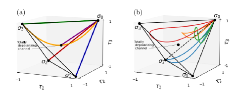
Figure 5: Some Pauli dynamical maps that can be implemented with a 1PR circuit. The curves painted in these tetrahedrons represent Pauli dynamical maps that can be implemented with 1PR circuits. (a) shows the dynamical maps mentioned in the main text, which are: depolarizing (purple), bit flip (blue), phase flip (green), bit-phase flip (red) and parabolic (orange). (b) shows dynamical maps selected at random that can be implemented with 1PR circuits.

• Depolarizing: This dynamical map is given by

  $$\varepsilon_{p}(\rho)=(1-3p/4)\rho+(p/4)\sigma_{1}\rho\sigma_{1}+(p/4)\sigma_{2}\rho\sigma_{2}+(p/4)\sigma_{3}\rho\sigma_{3},$$

  with $p\in[0,1]$. Therefore, the curve of states $|\beta(p)\rangle$ needed on the ancilla qubits is such that ${|\beta_{0}(p)|}^{2}=(1-3p/4)$, ${|\beta_{1}(p)|}^{2}={|\beta_{2}(p)|}^{2}={|\beta_{3}(p)|}^{2}=p/4$. Then, taking the $\beta_{j}$ to be real, the curve of states can be

  $$|\beta(p)\rangle=\sqrt{1-3p/4}|00\rangle+\sqrt{p/4}|01\rangle+\sqrt{p/4}|10\rangle+\sqrt{p/4}|11\rangle.$$

  This state can be rewritten as:

  $$|\beta(p)\rangle= \;e^{is}\left(\dfrac{1}{2}|00\rangle-\dfrac{i}{2\sqrt{3}}|01\rangle-\dfrac{i}{2\sqrt{3}}|10\rangle-\dfrac{i}{2\sqrt{3}}|11\rangle\right)$$

  $$+e^{-is}\left(\dfrac{1}{2}|00\rangle+\dfrac{i}{2\sqrt{3}}|01\rangle+\dfrac{i}{2\sqrt{3}}|10\rangle+\dfrac{i}{2\sqrt{3}}|11\rangle\right),$$

  with $\sin s=\sqrt{3p/4}$. We can see that this curve satisfies the conditions of Eq (25), meaning that it can be created with a 1PR circuit.

• Parabolic dynamical map: We define the parabolic dynamical map as:

  $$\epsilon(\rho)=\dfrac{1}{4}{(1-p)}^{2}\rho+\dfrac{1}{4}(1-p^{2})\sigma_{1}\rho\sigma_{1}+\dfrac{1}{4}(1-p^{2})\sigma_{2}\rho\sigma_{2}+\dfrac{1}{4}{(1+p)}^{2}\sigma_{3}\rho\sigma_{3},$$ (28)

  with $p\in[-1,1]$. If we take the $\beta_{j}$ to be real, the curve of states needed on the ancilla qubits can be:

  $$|\beta(p)\rangle=\dfrac{1}{2}(1-p)|00\rangle+\dfrac{1}{2}\sqrt{1-p^{2}}|01\rangle+\dfrac{1}{2}\sqrt{1-p^{2}}|10\rangle+\dfrac{1}{2}(1+p)|11\rangle.$$ (29)

  This can be rewritten as

  $$|\beta(p)\rangle= \;\left(\dfrac{1}{2}|00\rangle+\dfrac{1}{2}|11\rangle\right)+e^{is}\left(\dfrac{i}{4}|00\rangle+\dfrac{1}{4}|01\rangle+\dfrac{1}{4}|10\rangle-\dfrac{i}{4}|11\rangle\right)$$

  $$+e^{-is}\left(\dfrac{-i}{4}|00\rangle+\dfrac{1}{4}|01\rangle+\dfrac{1}{4}|10\rangle+\dfrac{i}{4}|11\rangle\right),$$

  with $\sin s=p$, so that this map fulfills the conditions of Eq (25).

• Bit flip map: This dynamical map is defined as

  $$\varepsilon_{p}(\rho)=(1-p)\rho+p\sigma_{1}\rho\sigma_{1},$$

  for $p\in[0,1]$. In particular, if we take the $\beta_{j}$ to be real, we need to create the curve of states:

  $$|\beta(p)\rangle=\sqrt{1-p}|00\rangle+\sqrt{p}|01\rangle.$$

  This can be rewritten as

  $$|\beta(p)\rangle=e^{is}\left(\frac{1}{2}|00\rangle-\dfrac{i}{2}|01\rangle\right)+e^{-is}\left(\frac{1}{2}|00\rangle+\frac{i}{2}|01\rangle\right),$$

  with $\sin s=\sqrt{p}$. Therefore, we can see that the curve satisfies the conditions of Eq (25) and it can be created with a 1PR circuit. Note that in this case we actually only need one ancilla qubit since the state $|\beta(p)\rangle$ is only two dimensional.

  The exact same thing can be done for the phase flip and bit phase flip dynamical maps by changing $\sigma_{1}$ to $\sigma_{3}$ and $\sigma_{2}$ respectively. For example, the bit phase flip map was implemented in [11, 35] using an optical arrangement, and it was indeed done by varying only one angle that depends on the parameter $p$ (the angle of a half waveplate).

Furthermore, we can construct other examples of Pauli dynamical maps such that they can be implemented with a 1PR circuit. To do it, we only need to choose the three states $|a\rangle$, $|b\rangle$, $|c\rangle$ that satisfy the conditions of Eq (25). For example, this can be done systematically for the case of curves of states of two qubits (that is, for Pauli dynamical maps of one qubit) with the following procedure:

• We first choose the norms $|a|$, $|b|$, $|c|$ such that $\langle a|a\rangle+\langle b|b\rangle+\langle c|c\rangle=1$. This can be done by selecting two angles $\mu\in[0,\pi/2]$, $\nu\in[0,\pi/2]$ and defining:

  $$|a|=\sin\nu\cos\mu,\;|b|=\sin\nu\sin\mu,\;|c|=\cos\nu.$$

• We define $|a^{\prime}\rangle=|a||0\rangle$, $|b^{\prime}\rangle=|b||1\rangle$, $|c^{\prime}\rangle=|c||2\rangle$.

• Finally, we choose a unitary matrix $V$ with the condition that its first row is equal to $e^{i\theta}(|a|,|b|,|c|,0)$ with $\theta$ a uniform random phase. That way, we can define $|a\rangle=V|a^{\prime}\rangle$, $|b\rangle=V|b^{\prime}\rangle$, $|c\rangle=V|c^{\prime}\rangle$ and since $V$ is unitary, these unprimed vectors will fulfill the conditions of Eq (25). Furthermore, the form of the first row ensures that the dynamical map begins at the identity, since it implies that when $s=0$, the state created in Eq (27) is $|a\rangle+|b\rangle+|c\rangle=e^{i\theta}|0\rangle$, which corresponds with applying the identity channel.

  Such a matrix $V$ can be randomly constructed by first finding three vectors $\vec{w}_{1},\vec{w}_{2},\vec{w}_{3}$ orthogonal to the first row using the Gram-Schmidt process. Then selecting random complex numbers $r_{1},r_{2},r_{3}$ such that $|r_{1}|^{2}+|r_{2}|^{2}+|r_{3}|^{2}=1$ and defining the second row of $V$ to be $r_{1}\vec{w}_{1}+r_{2}\vec{w}_{2}+r_{3}\vec{w}_{3}$. Once the first two rows are chosen, use Gram-Schmidt to find two vectors $\vec{v}_{1},\vec{v}_{2}$ orthogonal to them and similarly define the third row as $q_{1}\vec{v}_{1}+q_{2}\vec{v}_{2}$ with $|q_{1}|^{2}+|q_{2}|^{2}$ and $q_{1},q_{2}$ selected at random. Finally, there is only one choice for the fourth row so that it is orthonormal to the first three and a random phase can be given to it.

Following this procedure for random angles and unitary matrices $V$, we plot four Pauli dynamical maps selected at random that can be implemented with a 1PR circuit in Fig 5.

6 Conclusion

In this work, we found a quantum algorithm for simulating Pauli channels in $N$-qubit systems and generalized it to Pauli dynamical maps by using parametrized quantum circuits. Furthermore, we implemented single-qubit Pauli channels on one of IBM’s quantum computers and obtained their fidelities. Finally, when working with Pauli dynamical maps, we searched for a way of simplifying the parametrized circuit by requiring that only one single-qubit rotation depends on the parameter. In theorem 2 we found the general mathematical conditions for this, applicable to any parametrized circuit.

Therefore, this work presents yet another example of the current exploration into simulating open quantum systems in quantum computers, and we observe the big effect that the error of quantum computers have on these simulations. On the other hand, the result of theorem 2 shows what can be done with the condition of using only one parametrized rotation and can be applied to any quantum algorithm that requires parametrized circuits, such as those used for quantum machine learning.

7 Acknowledgments

Support by projects CONACyT 285754, and UNAM-PAPIIT IG101421 is acknowledged.

References

- 1. Feynman RP. Simulating physics with computers. Int J Theor Phys. 1982;21(6/7):467–488.
- 2. Zurek WH. Decoherence and the transition from quantum to classical. Phys Today. 1991;44(10):36–44.
- 3. Schlosshauer M. Decoherence, the measurement problem, and interpretations of quantum mechanics. Rev Mod Phys. 2005;76(4):1267–1305.
- 4. Breuer HP, Petruccione F. The theory of open quantum systems. 1st ed. New York: Oxford University Press; 2002.
- 5. García-Pérez G, Rossi M, Maniscalco S. IBM Q Experience as a versatile experimental testbed for simulating open quantum systems. npj Quantum Inf. 2020;6(1):1–11.
- 6. Wang H, Ashhab S, Nori F. Quantum algorithm for simulating the dynamics of an open quantum system. Phys Rev A. 2011;83(6):062317.
- 7. Weimer H, Kshetrimayum A, Orús R. Simulation methods for open quantum many-body systems. Rev Mod Phys. 2021;93(1):015008.
- 8. Xin T, Wei SJ, Pedernales JS, Solano E, Long GL. Quantum simulation of quantum channels in nuclear magnetic resonance. Phys Rev A. 2017;96(6):062303.
- 9. Wei S, Xin T, Long G. Efficient universal quantum channel simulation in IBM’s cloud quantum computer. Sci China Phys Mech Astron. 2018;61(7):70311.
- 10. Zanetti M, Pinto D, Basso M, Maziero J. Simulating noisy quantum channels via quantum state preparation algorithms. Phys B At Mol Opt Phys. 2023;56(11):115501.
- 11. Farías OJ, Aguilar GH, Valdés-Hernández A, Ribeiro PHS, Davidovich L, Walborn SP. Observation of the emergence of multipartite entanglement between a bipartite system and its environment. Phys Rev Lett. 2012;109(15):150403.
- 12. Aguilar GH, Valdés-Hernández A, Davidovich L, Walborn SP, Souto Ribeiro PH. Experimental entanglement redistribution under decoherence channels. Phys Rev Lett. 2014;113(24):240501.
- 13. Barreiro J, Müller M, Schindler P, Nigg D, Monz T, Chwalla M, et al. An open-system quantum simulator with trapped ions. Nature. 2011;470(7335):486–491.
- 14. Head-Marsden K, Krastanov S, Mazziotti D, Narang P. Capturing non-Markovian dynamics on near-term quantum computers. Phys Rev Res. 2021;3:013182.
- 15. Nielsen MA, Chuang IL. Quantum computation and quantum information: 10th anniversary edition. 10th ed. New York: Cambridge University Press; 2011.
- 16. Bengtsson I, Życzkowski K. Geometry of quantum states: an introduction to quantum entanglement. 1st ed. Cambridge: Cambridge University Press; 2006.
- 17. Puchała Z, Łukasz Rudnicki, Życzkowski K. Pauli semigroups and unistochastic quantum channels. Phys Lett A. 2019;383(20):2376–2381.
- 18. Davalos D, Ziman M, Pineda C. Divisibility of qubit channels and dynamical maps. Quantum. 2019;3:144.
- 19. Flammia S, Wallman J. Efficient estimation of Pauli channels. ACM Transactions on Quantum Computing. 2020;1(3):1–32.
- 20. Cerezo M, Arrasmith A, Babbush R, Benjamin SC, Endo S, Fujii K, et al. Variational quantum algorithms. Nat Rev Phys. 2020;3(9):625–644.
- 21. Benedetti M, Lloyd E, Sack S, Fiorentini M. Parameterized quantum circuits as machine learning models. Quantum Sci Technol. 2019;4(4):043001.
- 22. Rasmussen S, Loft N, Bækkegaard T, Kues M, Zinner N. Reducing the amount of single-qubit rotations in VQE and related algorithms. Adv Quantum Technol. 2020;3:2000063.
- 23. Rieffel E, Polak W. Quantum computing: a gentle introduction. 1st ed. Massachusetts: The MIT Press; 2011.
- 24. Heinosaari T, Ziman M. The Mathematical Language of Quantum Theory: From Uncertainty to Entanglement. 2nd ed. Cambridge: Cambridge University Press; 2012.
- 25. Wolf MM, Cirac JI. Dividing quantum channels. Comm Math Phys. 2008;279(1):147–168.
- 26. Choi MD. Completely positive linear maps on complex matrices. Linear Algebra Appl. 1975;10(3):285–290.
- 27. Jamiołkowski A. Linear transformations which preserve trace and positive semidefiniteness of operators. Rep Math Phys. 1972;3(4):275–278.
- 28. Marinescu D, Marinescu G. Classical and Quantum Information. 1st ed. Oxford: Elsevier; 2012.
- 29. Terhal BM. Quantum error correction for quantum memories. Rev Mod Phys. 2015;87(2):307–346.
- 30. Qiskit contributors. Qiskit: An Open-source Framework for Quantum Computing; 2023.
- 31. Chuang IL, Nielsen MA. Prescription for experimental determination of the dynamics of a quantum black box. J Mod Opt. 1997;44:2455–2467.
- 32. Wilde M. From classical to quantum Shannon theory. 2nd ed. Cambridge: Cambridge University Press; 2019.
- 33. Watrous J. Simpler semidefinite programs for completely bounded norms. Theor Comput Sci. 2013;19(8):1–19.
- 34. Benenti G, Strini G. Computing the distance between quantum channels: usefulness of the Fano representation. J Phys B At Mol Opt Phys. 2010;43(21):215508.
- 35. Aguilar GH, Farías OJ, Valdés-Hernández A, Souto Ribeiro PH, Davidovich L, Walborn SP. Flow of quantum correlations from a two-qubit system to its environment. Phys Rev A. 2014;89(2):022339.