General Anomaly Detection of Underwater Gliders
Validated by Large-scale Deployment Datasets

Abstract

Underwater gliders have been widely used in oceanography for a range of applications. However, unpredictable events like shark strikes or remora attachments can lead to abnormal glider behavior or even loss of the instrument. This paper employs an anomaly detection algorithm to assess operational conditions of underwater gliders in the real-world ocean environment. Prompt alerts are provided to glider pilots upon detecting any anomaly, so that they can take control of the glider to prevent further harm. The detection algorithm is applied to multiple datasets collected in real glider deployments led by the University of Georgia’s Skidaway Institute of Oceanography (SkIO) and the University of South Florida (USF). In order to demonstrate the algorithm generality, the experimental evaluation is applied to four glider deployment datasets, each highlighting various anomalies happening in different scenes. Specifically, we utilize high resolution datasets only available post-recovery to perform detailed analysis of the anomaly and compare it with pilot logs. Additionally, we simulate the online detection based on the real-time subsets of data transmitted from the glider at the surfacing events. While the real-time data may not contain as much rich information as the post-recovery one, the online detection is of great importance as it allows glider pilots to monitor potential abnormal conditions in real time.

I Introduction

Underwater gliders are extensively used in ocean research for activities such as ocean sampling, surveillance, and other purposes [1, 2, 3, 4, 5]. However, given the complexity of the ocean environment and the long-duration of glider missions, unexpected events such as shark attacks, wing loss, or attachment of marine species can cause gliders to operate abnormally or even totally fail [6, 7, 8]. In such cases, the gliders may drift to unexpected areas, making localization and rescue operations challenging. Furthermore, it can be difficult to detect the abnormal behavior of gliders, particularly when external disturbances arise, due to the lack of monitoring devices [9, 10, 11, 12]. The deployment of monitoring devices for gliders or the addition of self-monitoring of performance would increase mission costs and pilot complexity. Typically, glider pilots can only rely on heavily subsetted data transmitted by the glider in real time to form hypotheses about potential anomalies. Sometimes, they just resort to climb and dive ballast data to assess if the glider is surfacing or diving as expected. However, this empirical detection can never be conclusively confirmed as the mission is going on. To address this challenge, we develop an anomaly detection algorithm that systematically utilizes simple glider data such as glider speed, heading, and trajectory. This algorithm is feasible for theoretical validation on numerous real-world glider datasets, and runs autonomously in real-time, as opposed to manual detection by human pilots. By monitoring gliders in real-time, the algorithm allows glider pilots to take appropriate actions promptly to ensure the safety and success of missions.

Different strategies have been in the field of underwater robotics to identify abnormal behavior of underwater gliders. Some anomaly detection algorithms focus on changes in robot motion, such as roll angle or pitch angle, to detect possible motion deviation or a foreign object attached to the glider [13, 14]. Some algorithms monitor the power consumption or motor performance of the glider, as variations in these parameters can indicate degeneration of individual components, such as propellers and rotors [15, 16, 17]. Other algorithms utilize machine learning techniques to identify anomalous behavior by analyzing sensor data collected by the glider over time, such as changes in the speed, roll, pitch, or depth [18, 19, 20]. However, most of the existing research relies on shore-based manual implementations and does not resolve issues like inability to perform online detection on the gliders or lack of real-time experimental verification. In addition, it is essential to determine whether the detected anomaly is false positive [21, 22]. When the ocean current speed is significantly greater than the maximum speed of the marine robot, it can lead to a considerable performance degradation. Under such circumstances, false alarms should be avoided since the anomaly caused by an unexpected ocean current is unrelated to the glider itself. In practice, it is challenging to separate flow speed and glider speed due to hardware limitations, but leveraging the Controlled Lagrangian Particle Tracking (CLPT) framework [23], the anomaly detection algorithm in [24] generates real-time estimates of the glider speed and flow speed from the trajectory and heading angles. The estimated glider speed is compared with the normal speed range to detect anomalies, while the algorithm-estimated flow speed is compared with the glider-estimated flow speed to avoid false alarms.

We initially validate the anomaly detection algorithm by using two real-life deployment datasets [25]. Building upon this previous work, we aim to extend the algorithm to large-scale datasets, thus effectively handling various anomalies in diverse missions. We also plan to simulate online implementation of the detection to enable real-time interaction with glider pilots. This objectives constitute primary motivation of this paper, and our main contribution are summarized as follows.

• We demonstrate generality of the anomaly detection algorithm based on four glider datasets collected in real deployments featuring diverse anomalies.

• We simulate online mode implementation of the algorithm to a real glider deployment with limited data streams in real time for the first time.

The SouthEast Coastal Ocean Observing Regional Association (SECOORA) glider Franklin, operated by Skidaway Institute of Oceanography (SkIO), and the University of South Florida (USF) gliders USF-Sam, USF-Gansett, and USF-Stella provide numerous examples of valuable experimental data in which anomalies may be associated with marine bio-hazards. Promising anomaly detection results of these datasets are shown to well match glider pilots’ hindcast analysis. Building off its efficacy, the real-time anomaly detection algorithm is incorporated into the autonomous glider navigation software GENIoS_Python [26] to better assist human pilots as an add-on warning functionality.

This paper is organized as follows. Section II illustrates the framework of the anomaly detection algorithm. Section III describes the experimental setup of glider deployments, verifies the algorithm by detecting anomalies in large-scale real experiments, and simulates the online implementation on subsetted glider datasets. Section IV provides conclusions and future work.

II Anomaly Detection Algorithm

The pipeline of anomaly detection and false alarm elimination is shown in Fig. 1. By generating the glider speed estimate, the algorithm assumes no anomaly if the estimate is within the normal speed range. Otherwise, the glider may be encountering issues. The flow speed estimate is checked against the glider-estimated flow speed to circumvent any false alarm.

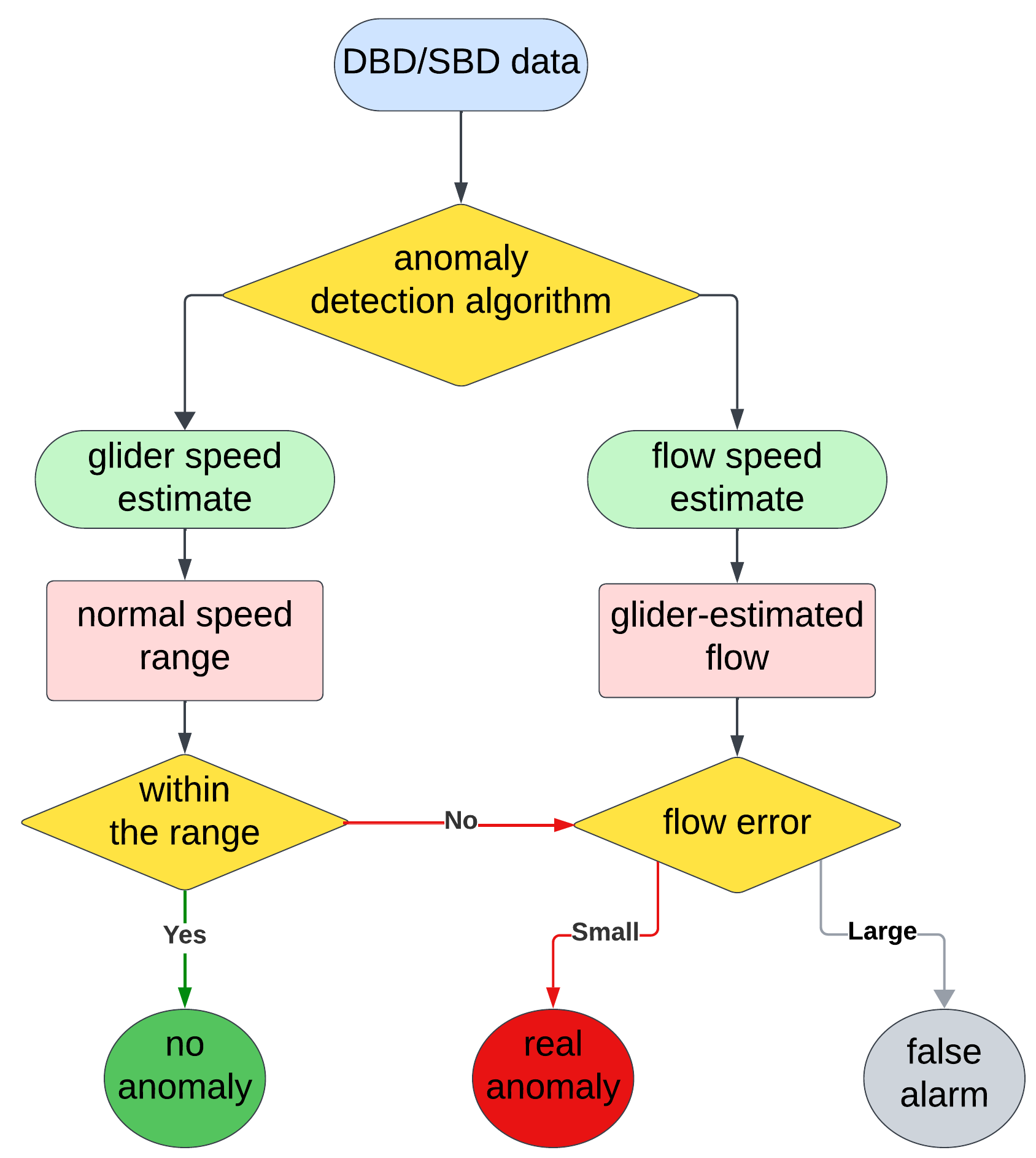
Figure 1: Pipeline of anomaly detection and false alarm elimination. Three steps: 1) generate glider speed estimate and flow speed estimate based on DBD or SBD data; 2) compare glider speed to detect anomalies; 3) compare flow speed for false alarm.

We model the glider dynamics as follows:

$$\dot{x}=F_{R}(x,t)+V_{R}(t)\Psi_{c}(t)$$

$$\Psi_{c}(t)=[\cos\psi_{c}(t),\sin\psi_{c}(t)]^{T},$$ (1)

where $F_{R}$ is the true flow field, $x$ is the true glider position, $V_{R}$ is the true glider speed, and $\psi_{c}$ is the true heading angle. As shown in (2), we model the ocean flow field by spatial-temporal basis functions [27],

$$F_{R}(x,t)=\theta\phi(x,t)$$ (2)

where $\theta$ is the unknown parameter to be estimated,

$$\phi=\begin{bmatrix}\phi^{1}(x,t)&\cdots&\phi^{N}(x,t)\end{bmatrix}^{T}$$ (3)

$$\phi^{i}(x,t)=\exp^{-\frac{||x-c_{i}||}{2\sigma_{i}}}\cos(\omega_{i}t+\upsilon_{i})$$ (4)

are the basis functions, $c_{i}$ is the center, $\sigma_{i}$ is the width, $\omega_{i}$ is the tidal frequency, $\upsilon_{i}$ is the tidal phase, and $N$ is the number of basis functions. Using the heading $\Psi_{c}(t)$ and the true trajectory $x(t)$, the detection algorithm can generate estimates of the glider speed $V_{R}$ and the unknown flow parameter $\theta$. These estimates will converge to true values as long as the maximum trajectory estimation error (CLLE) converges to zero. The heading data $\Psi_{c}(t)$ and the glider trajectory $x(t)$ are always available from full post-recovery Dinkum binary data (DBD) and typically included in subsetted short Dinkum binary data (SBD) sent in real-time. Three gains $K$, $\bar{\gamma}$ and $s$ are designed to accelerate the estimating process. If the estimated glider speed falls within an expected range $V_{L}(t)\in[V_{min},V_{max}]$, where the maximum glider speed $V_{max}$ and the minimum glider speed $V_{min}$ are defined a priori, no anomaly should have happened. Otherwise, the glider may not be operating normally. Additionally, introduce $F_{L}(t)$ as the algorithm-estimated flow speed, and $F_{M}(t)$ as the glider-estimated flow speed which can be generated by ocean models or sensor measurements. By defining a criteria $p_{E}$, we quantitatively evaluate the flow estimation error $||F_{M}(t)-F_{L}(t)||$ as

$$p_{E}=\frac{||F_{M}(t)-F_{L}(t)||}{2max(\hat{F}_{Lmax},\hat{F}_{Mmax})}$$ (5)

, where $\hat{F}_{Lmax}=max(||F_{L}(\tau)||_{\tau\in[0,t]})$ is the maximum algorithm-estimated flow speed until time $t$, and $\hat{F}_{Mmax}=max(||F_{M}(\tau)||_{\tau\in[0,t]})$ is the maximum glider-estimated flow speed until time $t$. If flow estimation error is too large ($p_{E}>\gamma_{f}$, where $\gamma_{f}$ is a pre-selected threshold), the detected anomaly is likely a false alarm.

III Experimental Evaluation

We apply the anomaly detection algorithm to four glider deployments across the coastal ocean of Florida and Georgia, USA. For evaluation, the anomaly detected by the algorithm is cross-validated by high-resolution glider DBD data and pilot notes. In particular, we simulate the online detection process on SBD data and compare the result with that detected from DBD data. For reference, the designed parameters are listed in TABLE I.

TABLE I: Designed parameters of experiments

Parameters	Franklin	USF-Sam	USF-Gansett	USF-Stella
number of basis functions N	4	4	4	4
width $\sigma_{i}$	13e3	50e3	32e3	30e3
tidal phase $\upsilon_{i}$	0	0	0	0
tidal frequency $\omega_{i}$	$2\pi$e-6	$2\pi$e-6	$2\pi$e-6	$2\pi$e-6
gain $K$	$\begin{bmatrix}0.003&0\\ 0&0.003\end{bmatrix}$	$\begin{bmatrix}0.002&0\\ 0&0.002\end{bmatrix}$	$\begin{bmatrix}0.003&0\\ 0&0.003\end{bmatrix}$	$\begin{bmatrix}0.003&0\\ 0&0.003\end{bmatrix}$
gain $\bar{\gamma}$	5e-7	5e-7	1e-6	1e-7
gain $s$	30e-3	7e-3	18e-3	30e-3
false alarm threshold $\gamma_{f}$	1.0	1.0	1.0	1.0
maximum glider speed $V_{max}$	0.25	0.25	0.25	0.25
minimum glider speed $V_{min}$	0.15	0.15	0.15	0.15

III-A Experimental Setup

All the gliders used in the experiments are Slocum gliders, which are a type of autonomous underwater vehicles (AUVs) that move by adjusting buoyancy and center of gravity [28]. These gliders are able to perform ocean surveying for months by traveling at $0.25–0.35m\cdot s^{-1}$. During the mission, the gliders surface at fixed intervals (usually four hours) to transmit lightweight SBD datasets to the on-shore dockserver. It also estimates the average flow speed through dead reckoning. Post recovery, all the datasets are downloaded off the glider and stored as DBD files. The anomaly detection algorithm in Section II is applied to post-recovery DBD data and real-time SBD data in the offline and online mode, respectively, and verified by both the sensor data segments and the glider pilots’ notes.

The deployment details of four glider deployments are shown in TABLE II along with the Google Earth trajectories in Fig. 2. It is worth mentioning that USF-Sam is piloted under the support of GENIoS_Python [26] in real time, and USF-Sam is simulated by the online detection algorithm to report any potential anomaly.

TABLE II: Deployment details

Deployments	Time (UTC)	Area	Mission distance	Glider team	Algorithm
Franklin	Oct. 08 - Nov. 01, 2022	Savannah, Georgia	600 km	SkIO	Anomaly Detection
USF-Sam	Feb. 25 - Mar. 27, 2023	Gray’s Reef	610 km	USF	Anomaly Detection & GENIoS_Python
USF-Gansett	Nov. 10 - Dec. 8, 2021	Tampa Bay, Florida	1100 km	USF	Anomaly Detection
USF-Stella	Mar. 24 - May 09, 2023	Clearwater, Florida	400 km	USF	Anomaly Detection

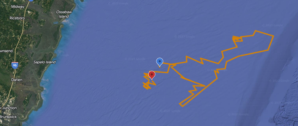
(a) Google Earth trajectory for the 2022 Franklin deployment.

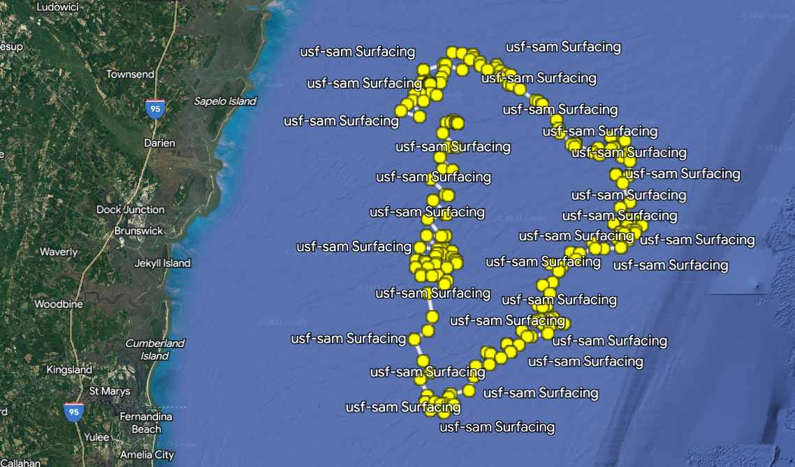
(b) Google Earth trajectory for the 2023 USF-Sam deployment.

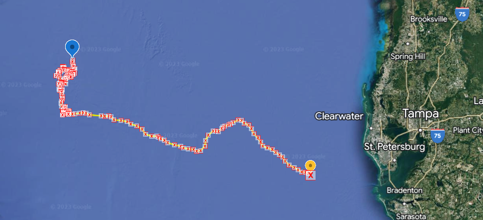
(c) Google Earth trajectory for the 2021 USF-Gansett deployment.

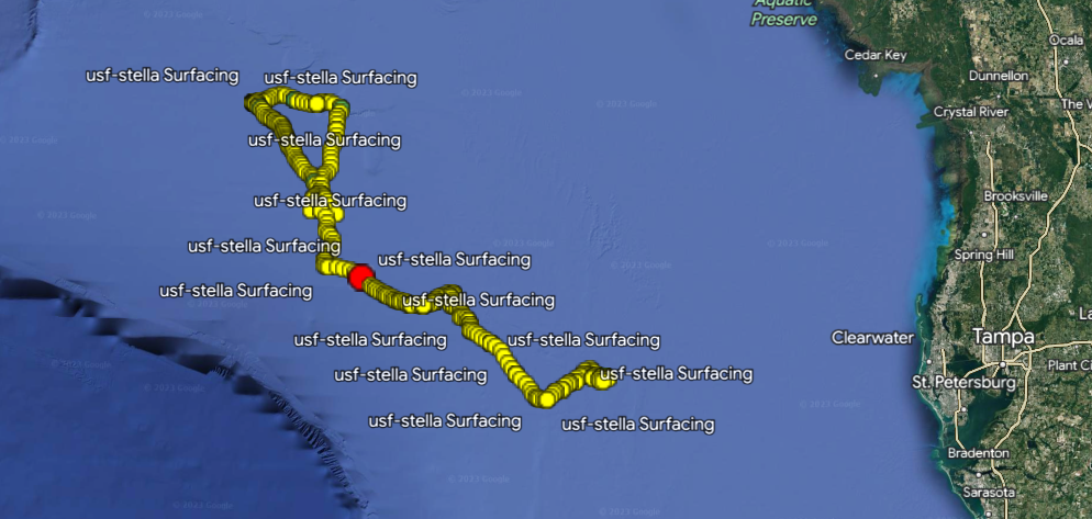
(d) Google Earth trajectory for the 2023 USF-Stella deployment.

Figure 2: Google Earth trajectories of glider deployments

III-B Large-scale Experiments

The large-scale experiments apply hindcast anomaly detection to full resolution DBD files downloaded from the glider on the shore. For verification, the algorithm-detected anomaly is compared with that directly seen from post-mission DBD data with the highest possible resolution and pilot logs.

III-B1 Franklin

From October 12 to October 13, 2022, Franklin experienced two aborts and delays of up to 40 minutes of subsequent surfacings. The glider pilot time believed that Franklin had attracted remoras or had encountered an obstruction on his port wing, resulting in a roll change shown in Fig. 3(a). Its climb to the ocean surface is unexpectedly slow even though flying with climb ballast near the upper limits of extended buoyancy pump, as shown in Fig. 3(b).

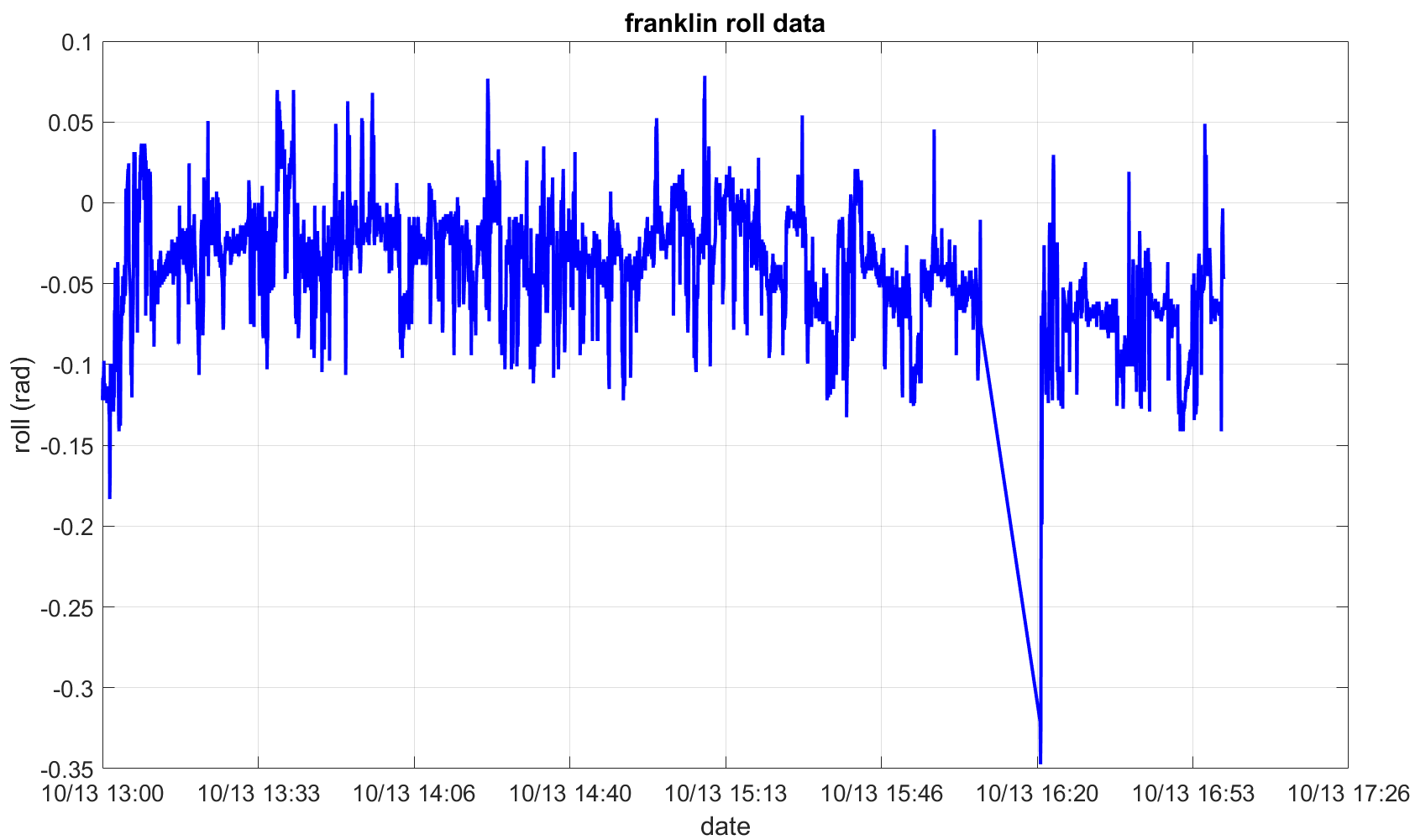
(a) Glider-measured roll (rad) from post-recovery DBD data.

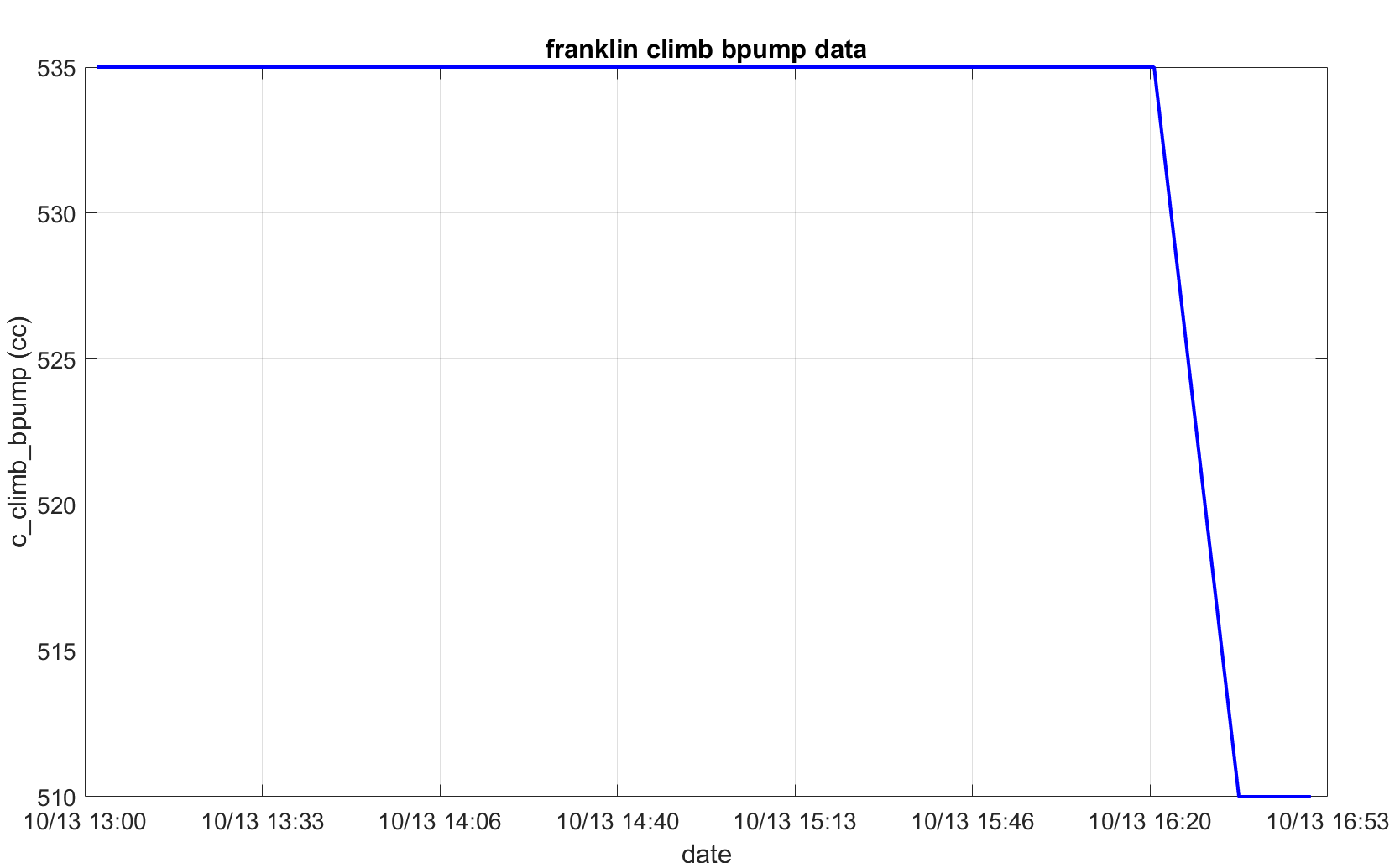
(b) Glider-measured climb ballast (cc) from post-recovery DBD data.

Figure 3: ground truth for the 2022 Franklin deployment.

Applied to the DBD data downloaded from the glider, the detection algorithm guarantees convergence of the estimated trajectory to the true trajectory as shown in Fig. 4. There are four basis functions (four green circles) covering the glider trajectory in the whole flow fields, which is an essential condition for parameter estimation to converge. As shown in Fig. 5, the maximum CLLE is small enough as $2.5m$, considering the glider moves hundreds of kilometers in the entire deployment, so we can also conclude the convergence of CLLE.

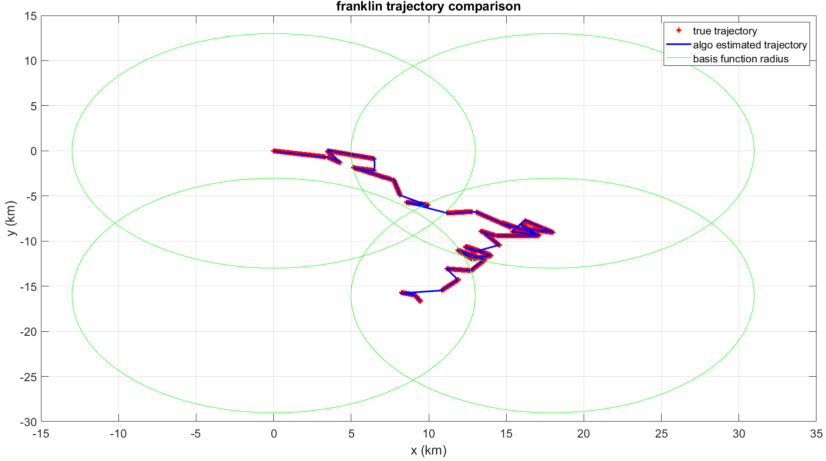
Figure 4: Comparison of the estimated (blue) and true (red) trajectory for the 2022 Franklin deployment. The four green circles are the four basis functions covering the whole trajectory.

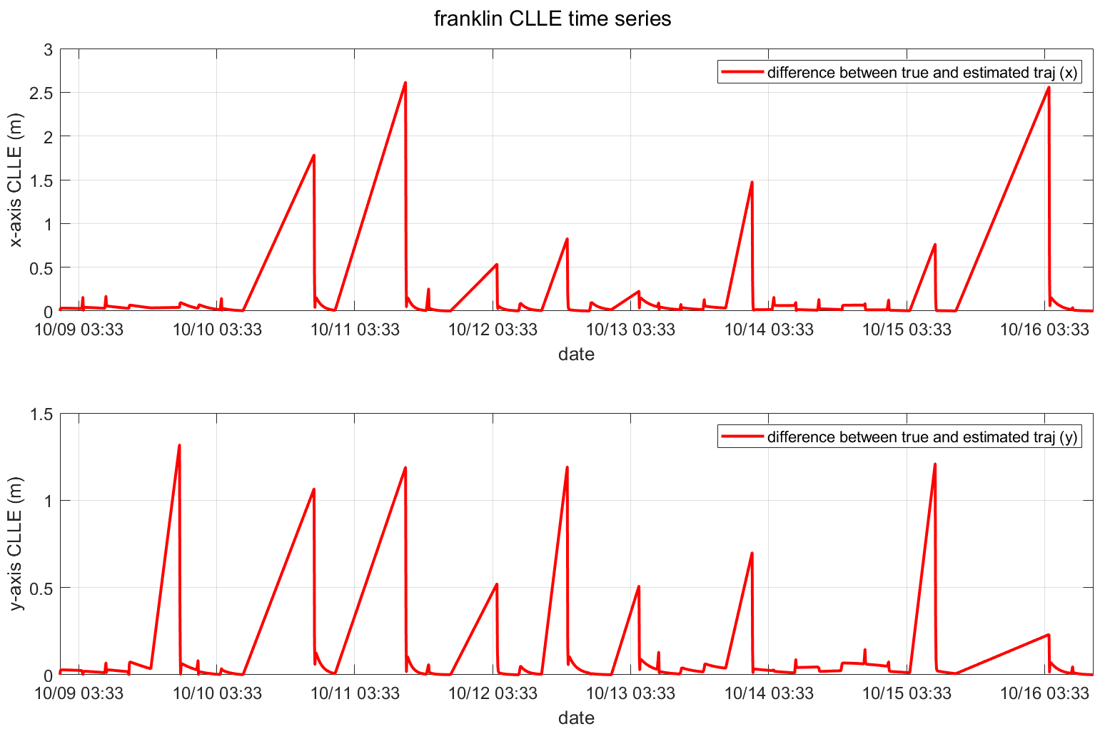
Figure 5: CLLE (m) for the 2022 Franklin deployment.

The CLLE convergence guarantees the convergence of both the glider speed estimate and the flow speed estimate. For precise comparison, the flow is divided into its West-East (W-E or zonal) component, denoted as $u$, and its North-South (N-S or meridional) component, denoted as $v$. The graphs in Fig. 6(a) demonstrate that the algorithm-estimated W-E flow is close to the corresponding glider estimate, indicating minimal error in the $u$ flow estimation. A similar comparison can be observed for the N-S flow, as shown in Fig. 6(b). This comparative analysis provides reliability of the anomaly detection when it is triggered. If the estimated glider speed drops out of the normal speed range, the anomaly should have occurred. As shown in Fig. 7, the estimated glider speed drops out of the normal speed range (green dot line) at around October 13, 2022, 15:00 UTC. The timestamp when the anomaly is detected by the algorithm corresponds to the timestamp detected from the glider team’s report and the post-recovery DBD data. Therefore, the algorithm is verified by successfully detecting the anomaly.

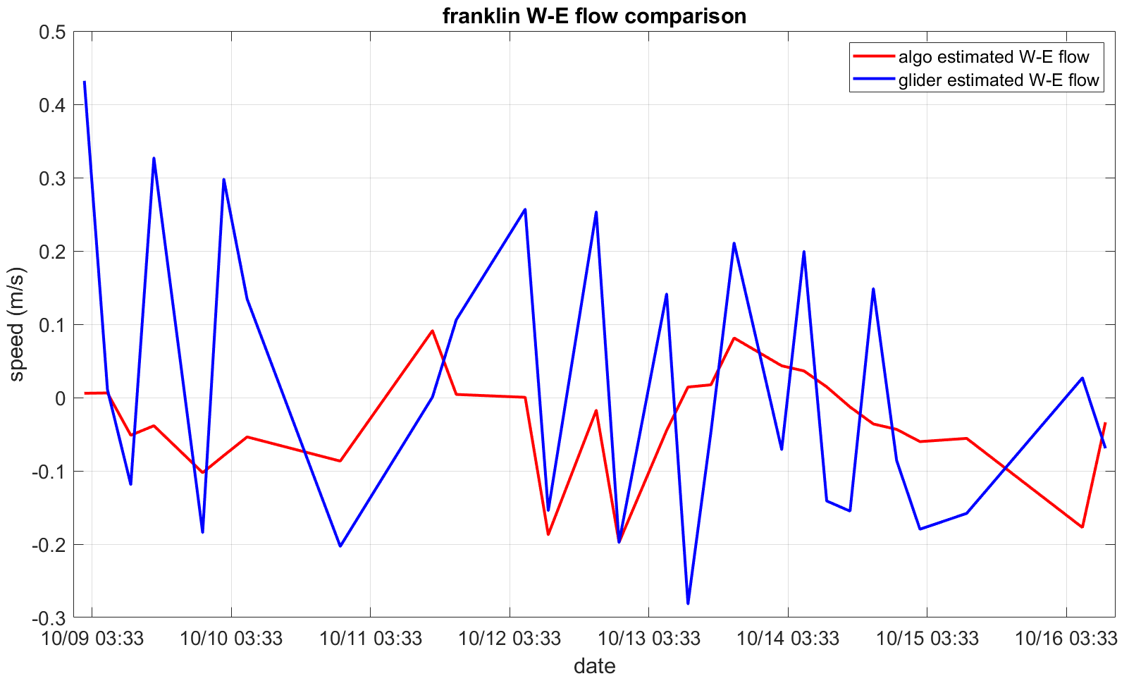
(a) W-E flow component.

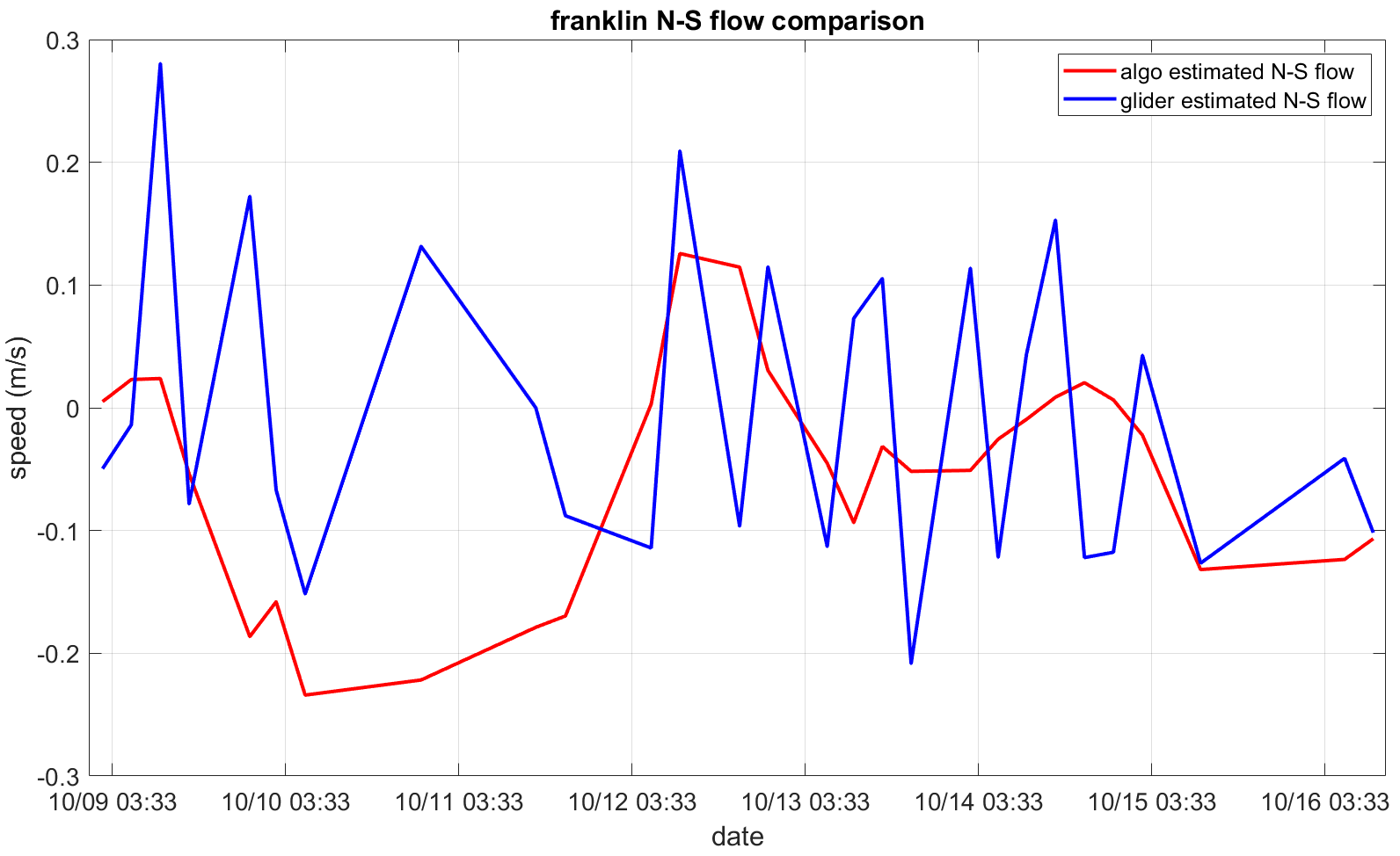
(b) N-S flow component.

Figure 6: Comparison of glider-estimated and algorithm-estimated W-E ($u$, upper) and N-S ($v$, lower) flow velocities for the 2022 Franklin deployment.

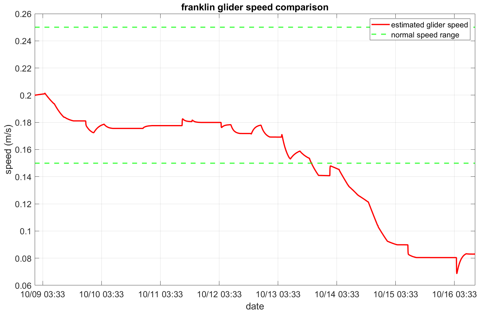
Figure 7: Comparison of estimated glider speed (red) and normal speed range (green) for the 2022 Franklin deployment.

III-B2 USF-Sam

During the mission, glider pilots suggest that the remora attachment should occur between March 11 and March 12, 2023 UTC when USF-Sam has a couple of roll and pitch changes shown in Fig. 8(a) and Fig. 8(b). This suggestion is reinforced by USF-Sam’s prolonged period of being stuck at a certain depth.

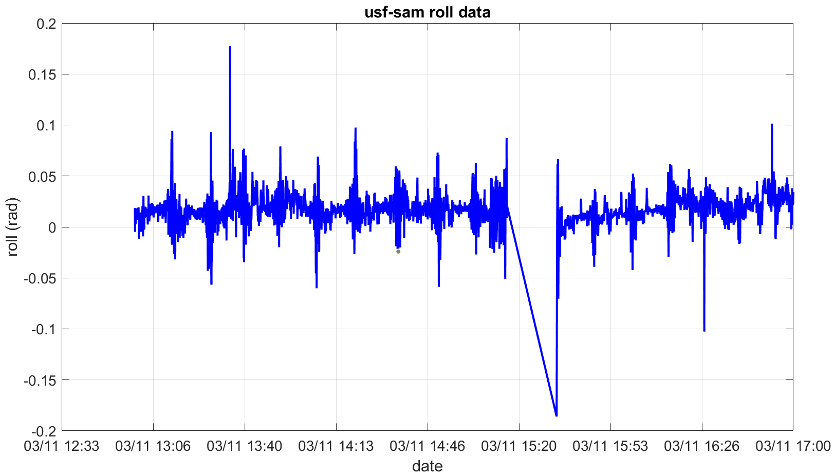
(a) Glider-measured roll (rad) from post-recovery DBD data.

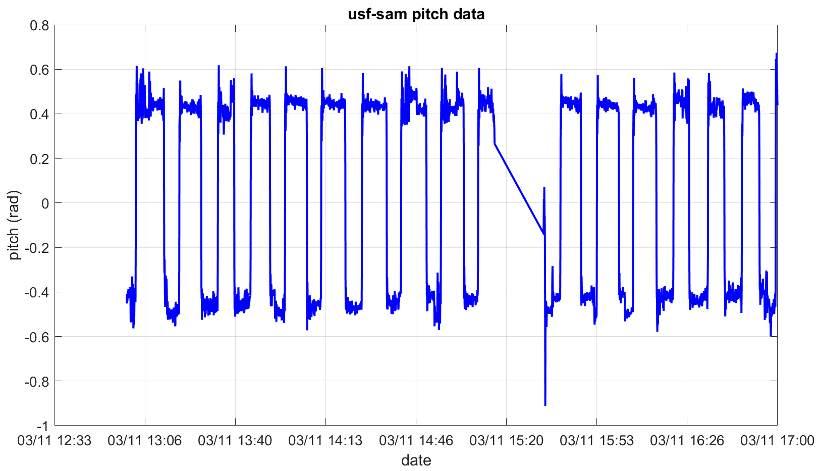
(b) Glider-measured pitch (rad) from post-recovery DBD data.

Figure 8: ground truth for the 2023 USF-Sam deployment.

Based on the DBD data, the detection algorithm generates the estimated trajectory, which is close to the true trajectory as shown in Fig. 9. From quantitative analysis in Fig. 10, the maximum CLLE $45m$ is small enough to conclude the CLLE convergence. We follow the same process of evaluating flow estimation error in Section III-B1. As shown in Fig. 11, the small flow estimation error suggests that the detection result can be trusted. As shown in Fig. 12, the estimated glider speed drops out of the normal speed range (green dot line) at around March 11, 2023, 20:00 UTC. The timestamp when the anomaly is detected by the algorithm corresponds to the timestamp detected from the glider team’s report and the DBD dataset.

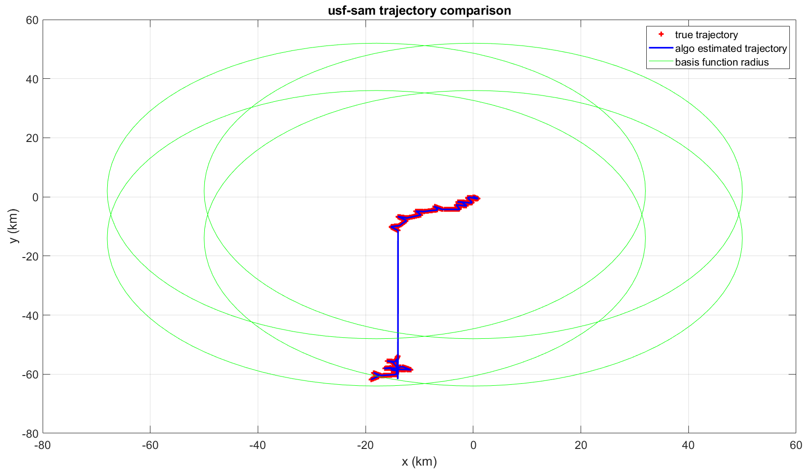
Figure 9: Comparison of the estimated (blue) and true (red) trajectory for the 2023 USF-Sam deployment. The four green circles are the four basis functions covering the whole trajectory.

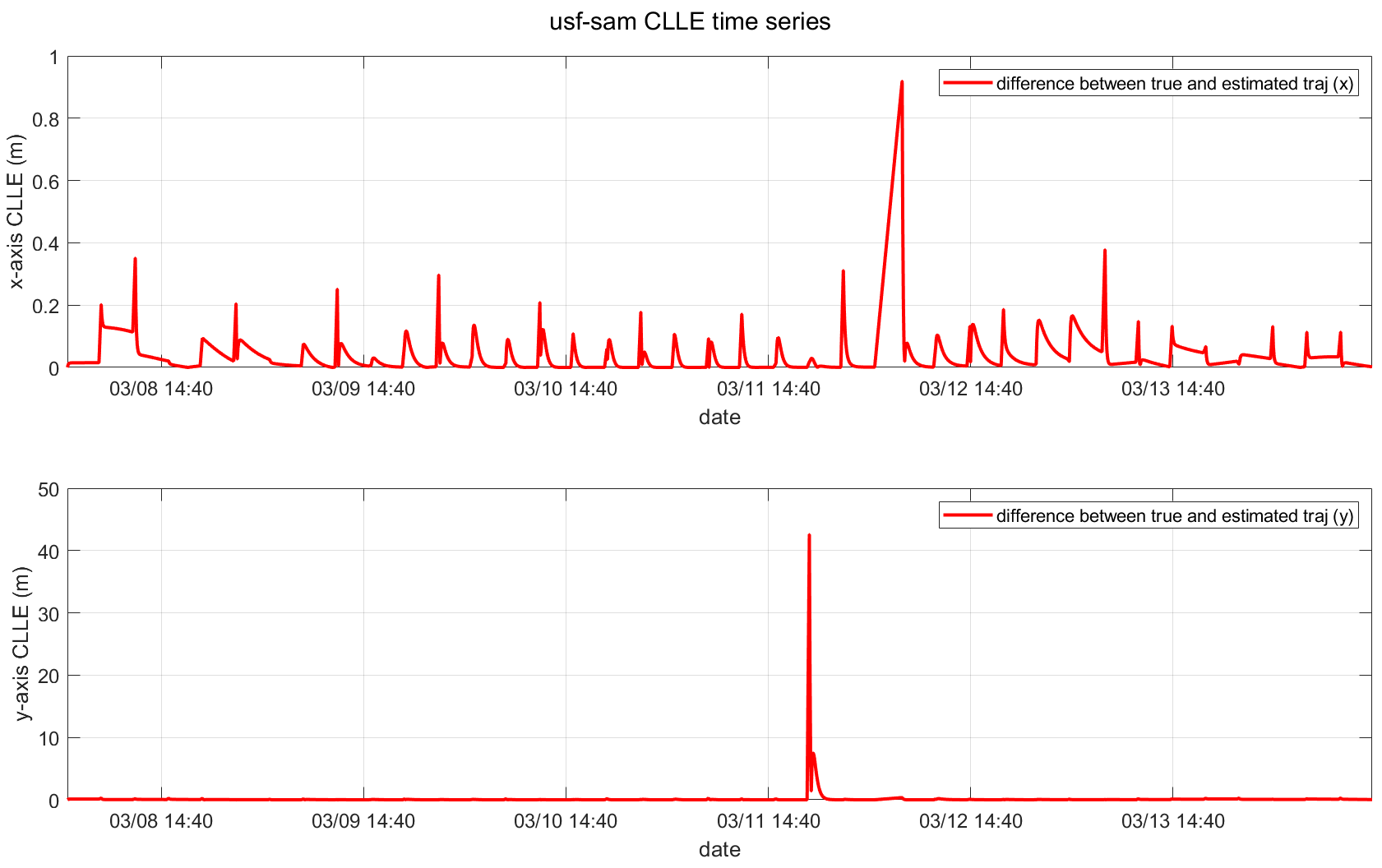
Figure 10: CLLE (m) for the 2023 USF-Sam deployment.

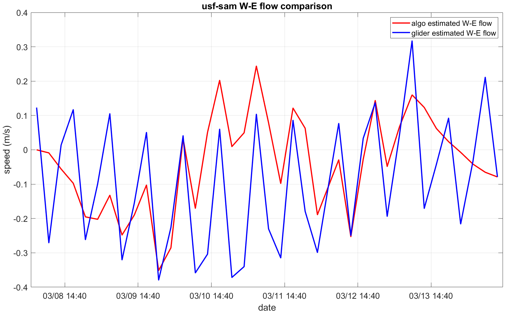
(a) W-E flow component.

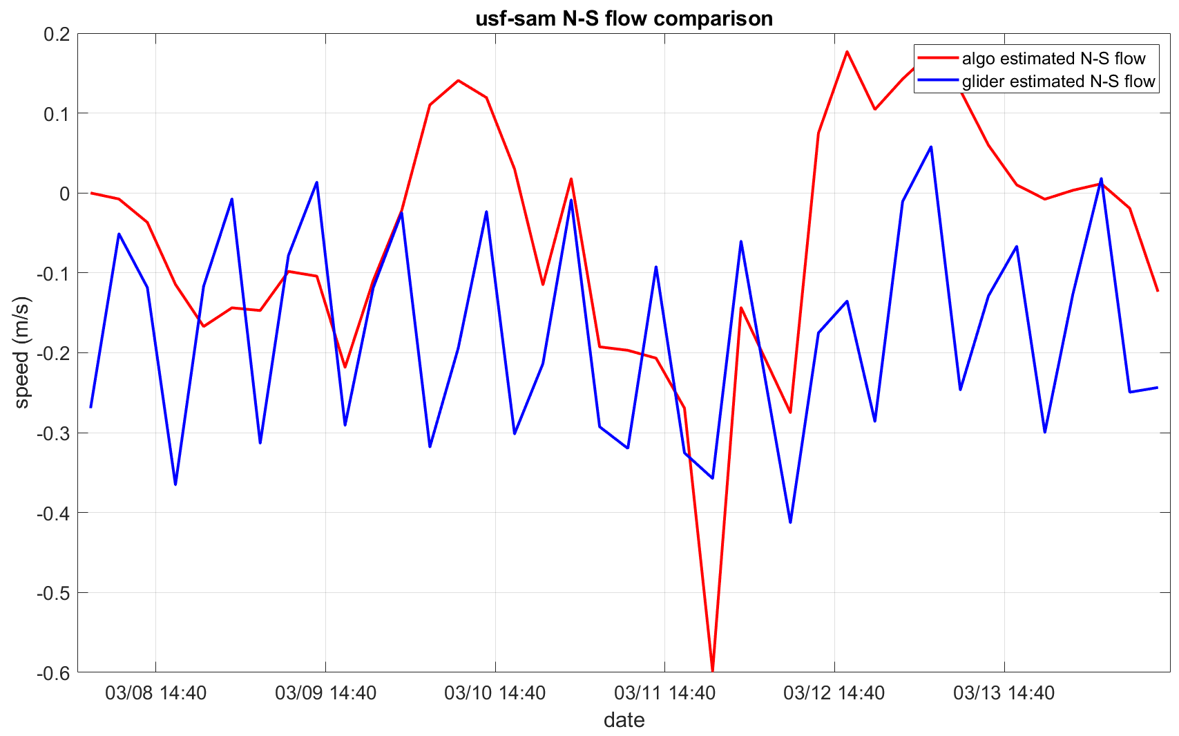
(b) N-S flow component.

Figure 11: Comparison of glider-estimated and algorithm-estimated W-E ($u$, upper) and N-S ($v$, lower) flow velocities for the 2023 USF-Sam deployment.

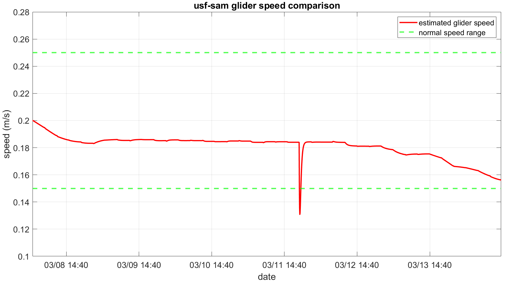
Figure 12: Comparison of estimated glider speed (red) and normal speed range (green) for the 2023 USF-Sam deployment.

The simulated online experiment implements anomaly detection using subsetted real-time SBD files transmitted from the glider to the dockserver during the mission. For example, the SBD file may contain fewer than 30 variables at 18-1800 s intervals, and is often subsampled to every 3rd or 4th yo (or down-up cycle), compared to the approximately 3000 variables stored at approximately 1 s interval on every yo in the DBD file processed on shore. The algorithm fetches new SBD files from the dockserver, parses SBD data from the SBD files, and applies the detection algorithm to the SBD data in an online mode. The online detection holds unique significance from the perspective that the detection results could help pilots monitor glider conditions in real time, thus circumventing any further loss and DBD data anomaly is only available post recovery.

Instead of waiting for the DBD data after the entire mission, the online detection is capable of utilizing the SBD data in real time. As shown in Fig. 13, the detection algorithm can also achieve trajectory convergence similar to using the DBD data. The maximum CLLE $5m$ in Fig. 14 is sufficiently small given the glider moving range in the ocean. Therefore, we can conclude the CLLE convergence. We follow the same process of evaluating flow estimation error in Section III-B1. As shown in Fig. 15, the small flow estimation error suggests that the online detection result is trustworthy. As shown in Fig. 16, the estimated glider speed drops out of the normal speed range (green dot line) at around March 12, 2023, 03:00 UTC. This result matches reasonably well the above result from the DBD data, which justifies that we can trust the online anomaly detection applied to real-time SBD data.

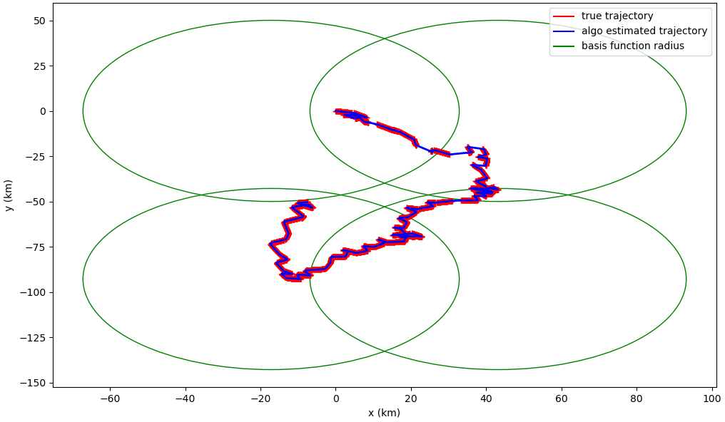
Figure 13: Comparison of the estimated (blue) and true (red) trajectory for the 2023 USF-Sam deployment based on real-time SBD data. The four green circles are the four basis functions covering the whole trajectory.

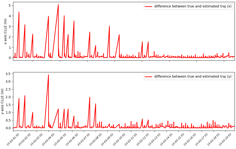
Figure 14: CLLE (m) for the 2023 USF-Sam deployment based on real-time DBD data.

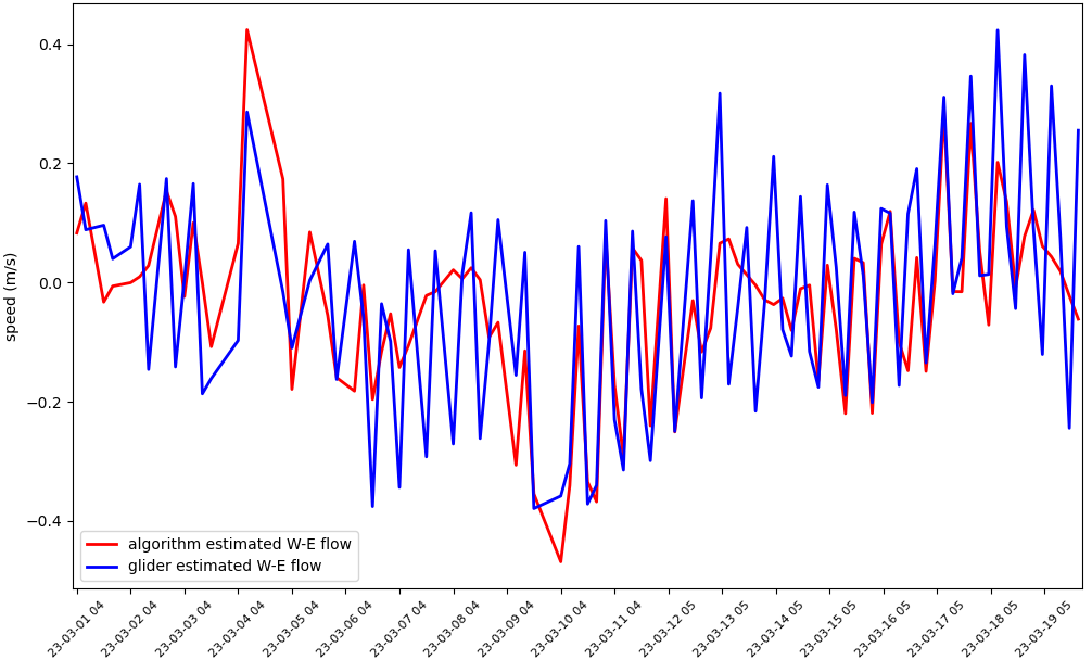
(a) W-E flow component.

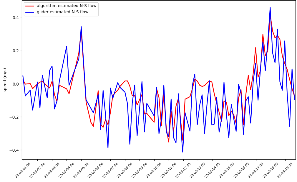
(b) N-S flow component.

Figure 15: Comparison of glider-estimated and algorithm-estimated W-E ($u$, upper) and N-S ($v$, lower) flow velocities for the 2023 USF-Sam deployment based on real-time SBD data.

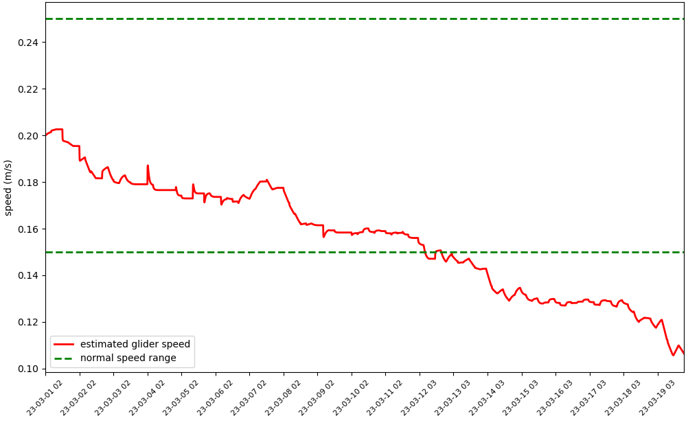
Figure 16: Comparison of estimated glider speed (red) and normal speed range (green) for the 2023 USF-Sam deployment based on real-time SBD data.

III-B3 USF-Gansett

At November 12, 2021, 22:32 UTC, the glider USF-Gansett sharply rolled to starboard $47\degree$ and pitches to $54\degree$, settling back by 22:36 UTC to a roll of $11\degree-15\degree$ and normal pitches as shown in Fig. 17(a) and Fig. 17(b). Heading changes during this time also varied by over $100\degree$ as shown in Fig. 17(c). This abnormal roll persisted even though pitch and heading returns to normal afterwards.

Upon recovery, gouges resembling teeth marks are evident on the aft hull and science bay as shown in Fig. 18(a). The arc of the marks span approximately 9 inches. The chord between the top and bottom ends of the aft hull markings is approximately 7.5 inches. The netting on the hull was cut in numerous areas, suggesting a serious shark strike. It is highly hypothesized that the bent starboard wing in Fig. 18(b) is caused by the shark strike.

(a) Glider-measured roll (rad) from post-recovery DBD data.

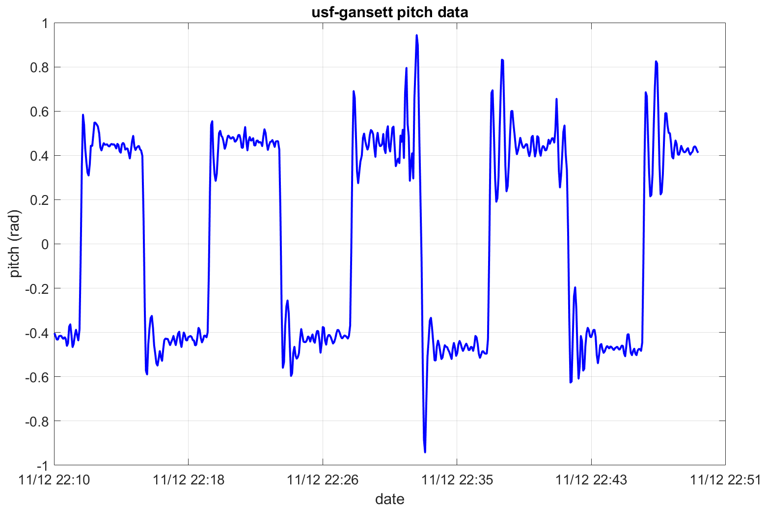
(b) Glider-measured pitch (rad) from post-recovery DBD data.

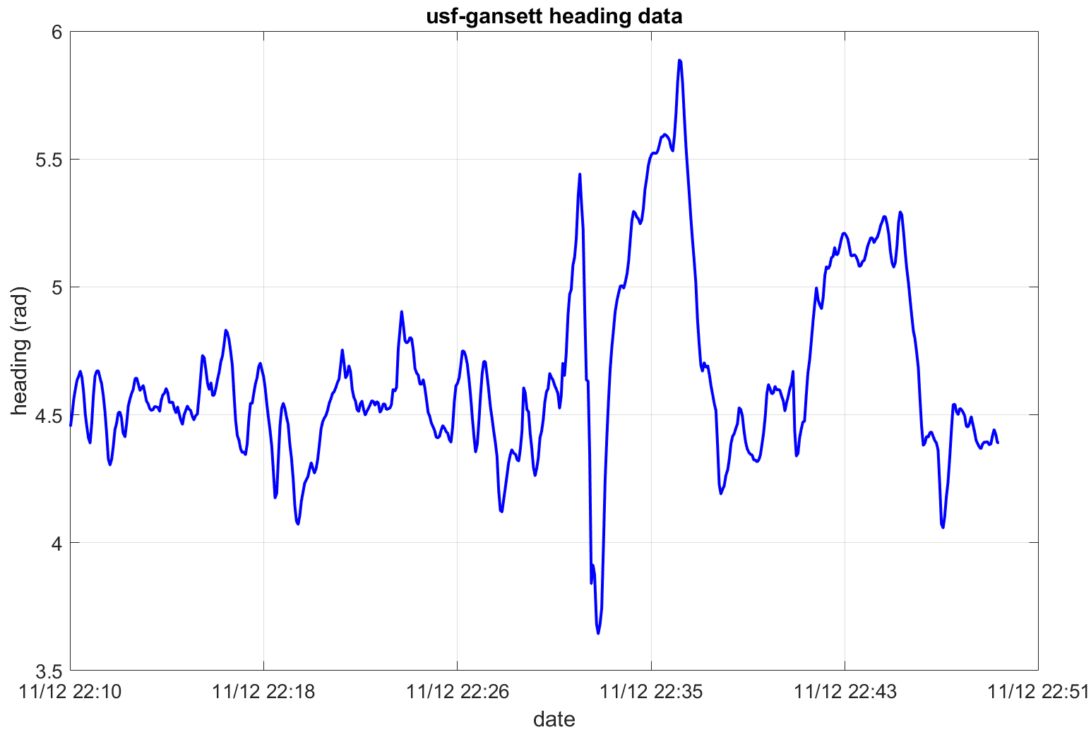
(c) Glider-measured heading (m) from post-recovery DBD data.

Figure 17: Ground truth for the 2021 USF-Gansett deployment.

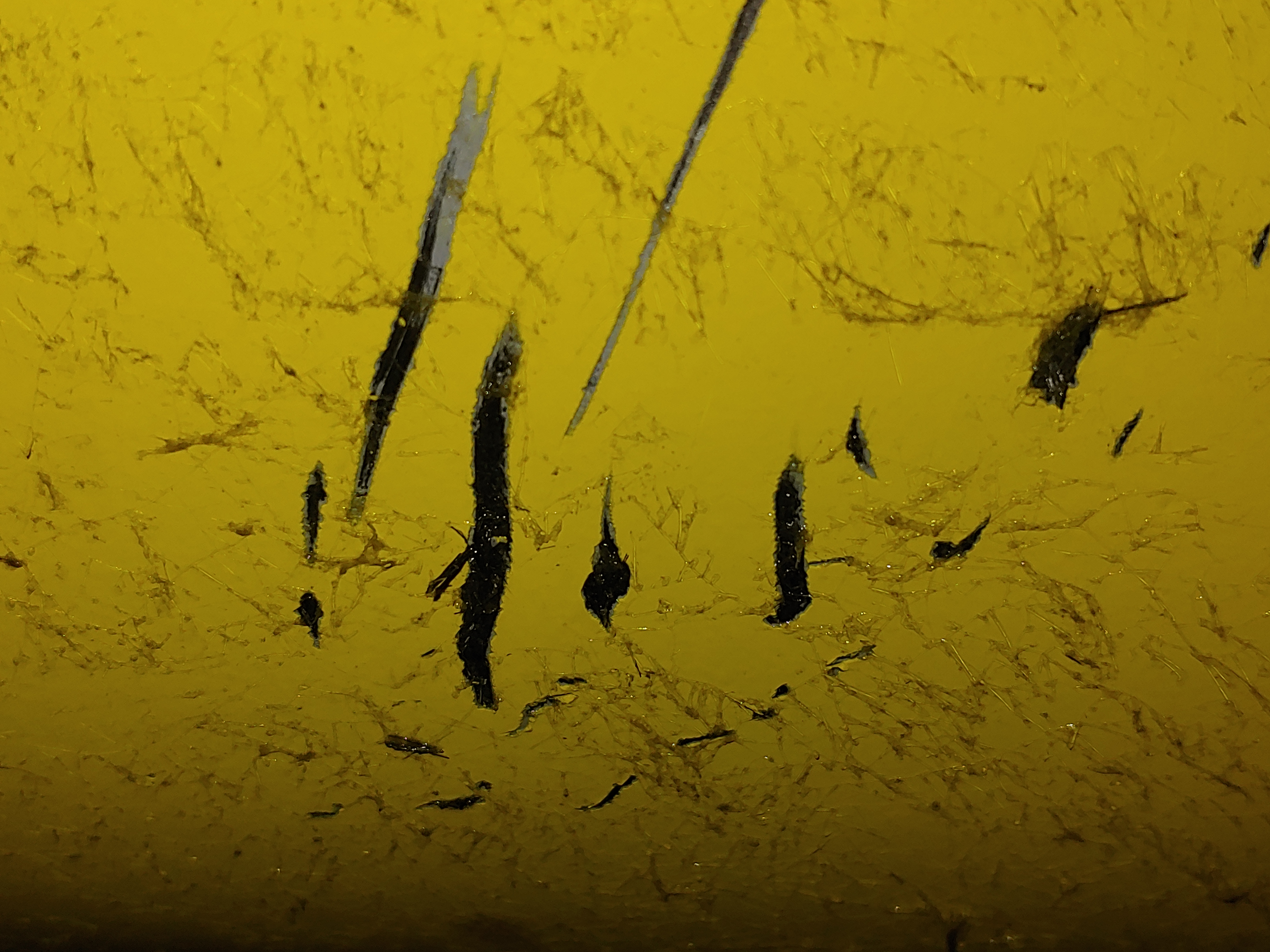
(a) Teeth marks on the aft hull of USF-Gansett

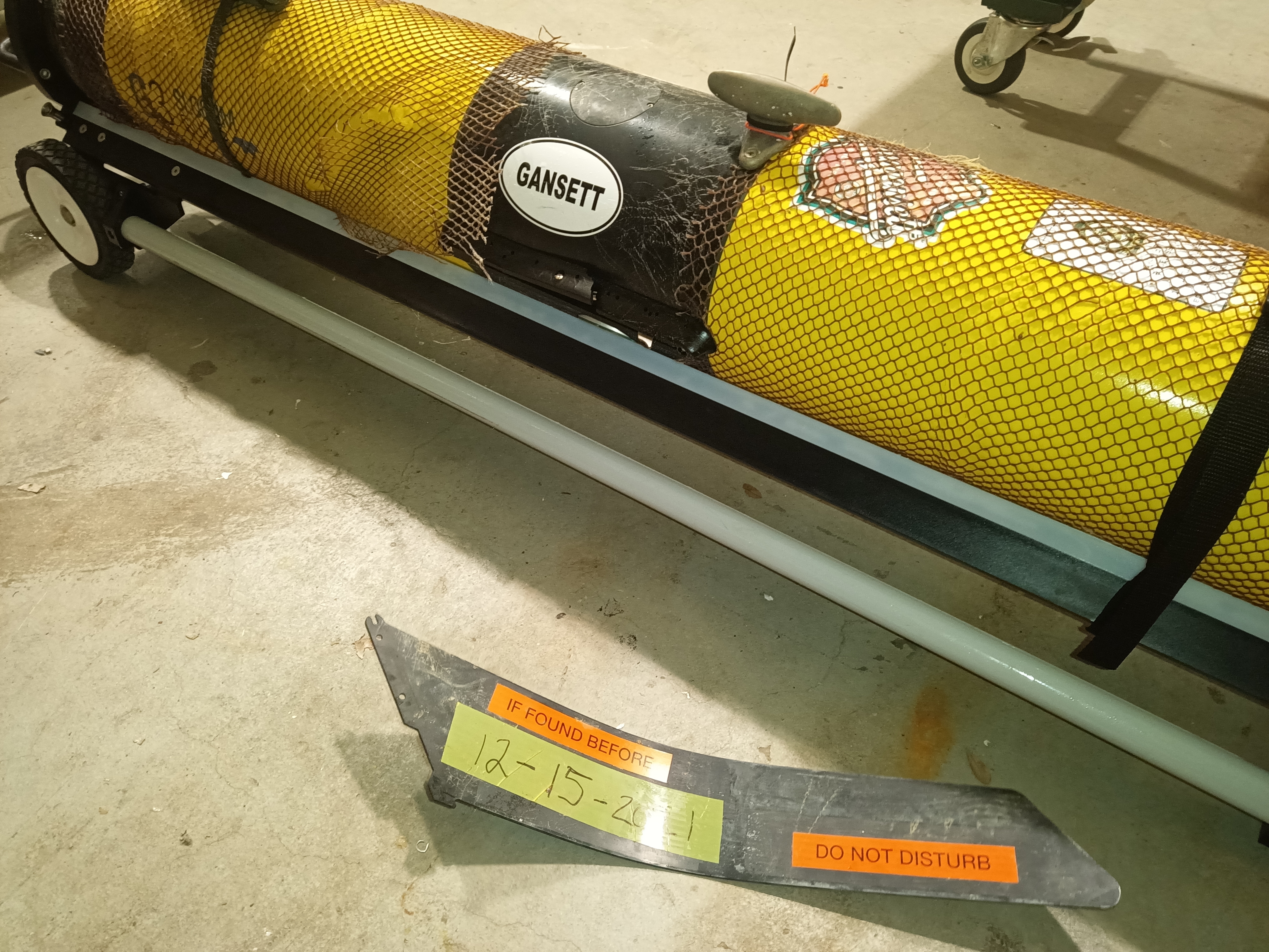
(b) Bent wing and cut netting upon recovery.

Figure 18: Post-recovery evidence of shark strike on USF-Gansett

Based on the DBD data, the estimated trajectory is close to the true trajectory as shown in Fig. 19. From quantitative analysis in Fig. 20, the maximum CLLE $1.1m$ is small enough to conclude the CLLE convergence. We follow the same process of evaluating flow estimation error in Section III-B1. As shown in Fig. 21, the small flow estimation error suggests that the detection result can be trusted. As shown in Fig. 22, the estimated glider speed dropped out of the normal speed range (green dot line) at around November 12, 2021, 22:00 UTC, followed by radical speed changes that match the persistent roll change in the glider team’s report. The timestamp when the anomaly is detected by the algorithm corresponds to the timestamp hypothesised by the glider team.

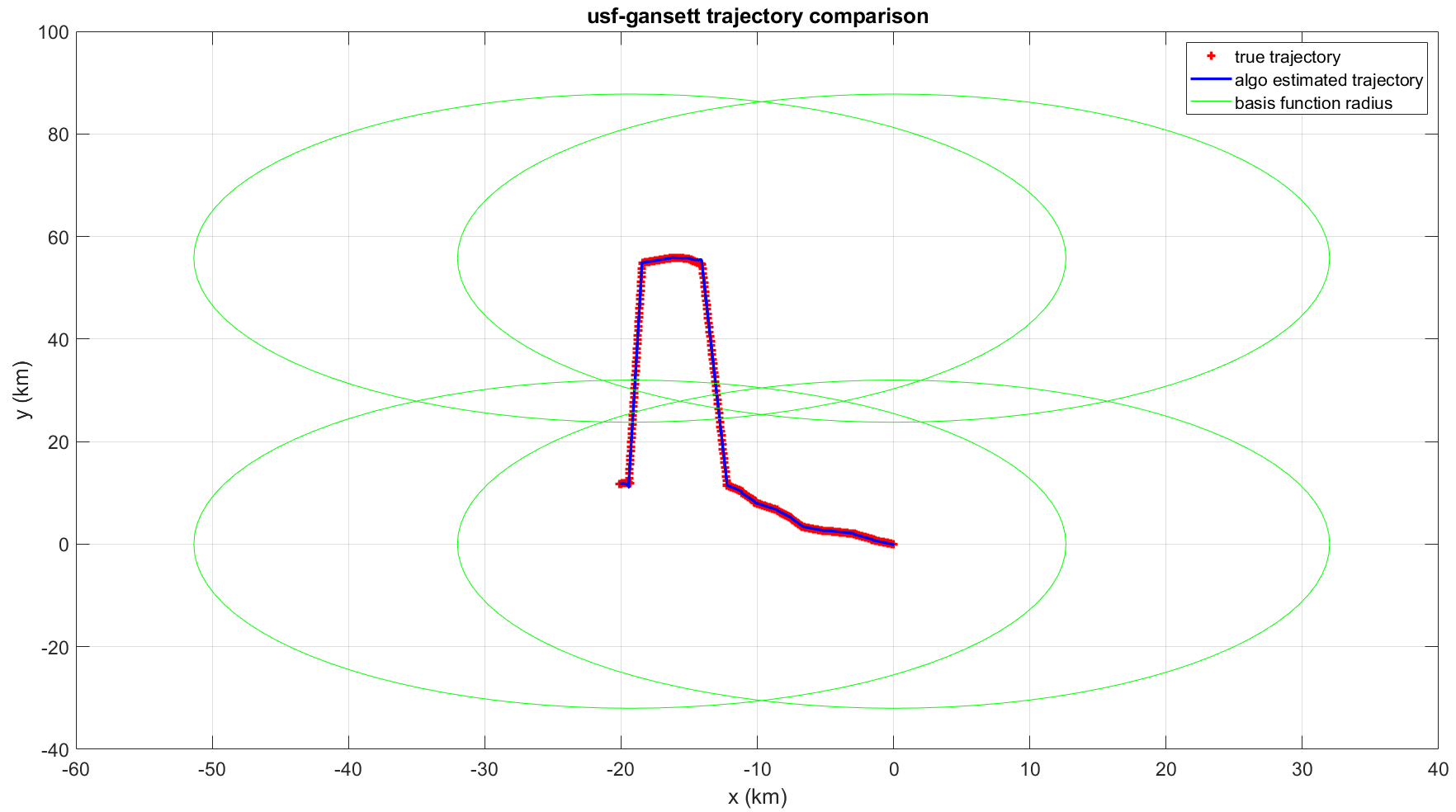
Figure 19: Comparison of the estimated (blue) and true (red) trajectory for the 2021 USF-Gansett deployment. The four green circles are the four basis functions covering the whole trajectory.

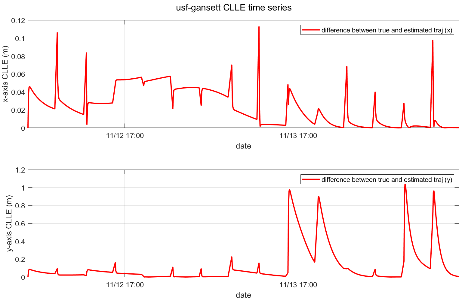
Figure 20: CLLE (m) for the 2021 USF-Gansett deployment.

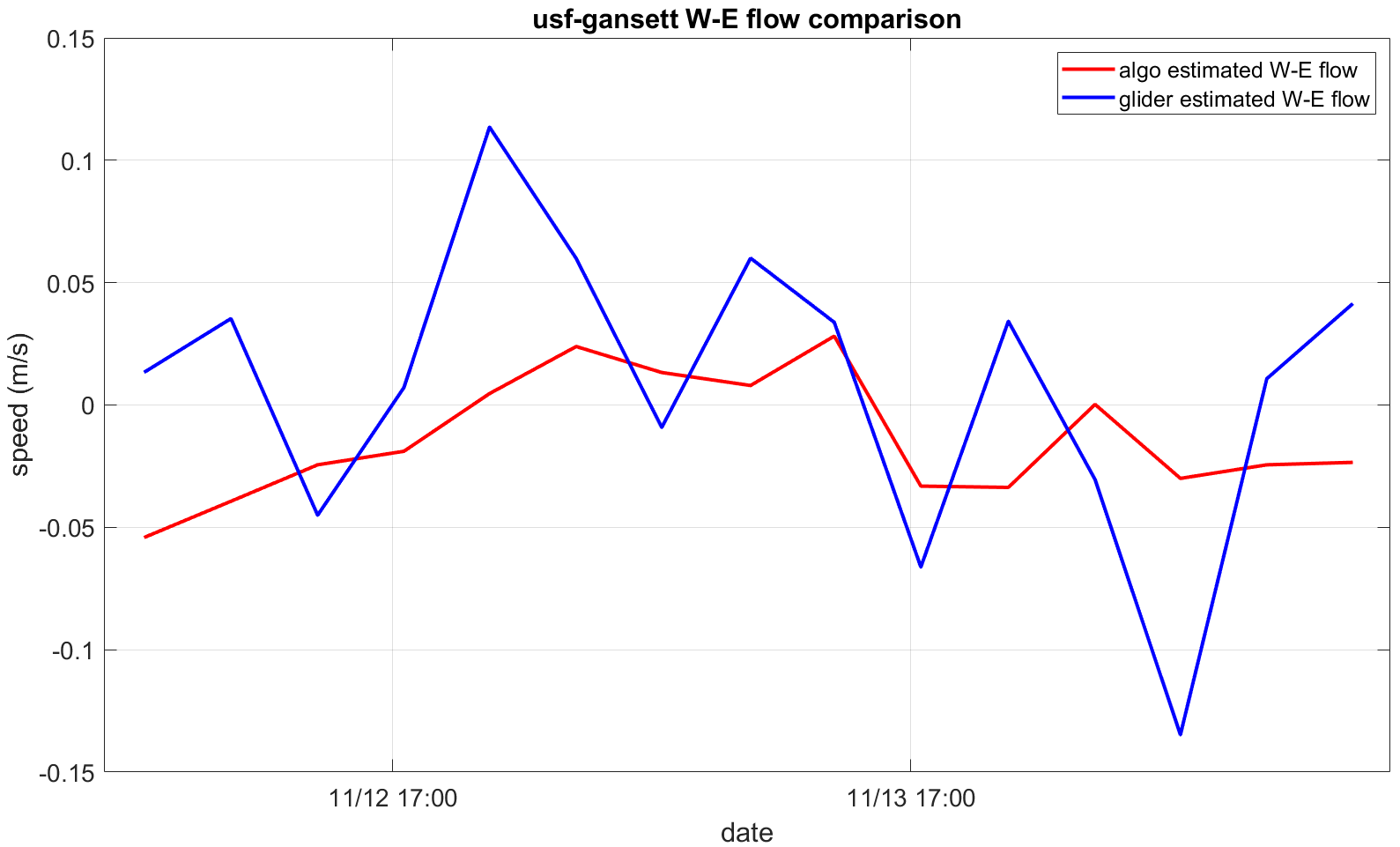
(a) W-E flow component.

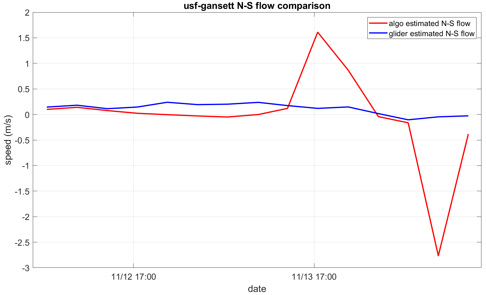
(b) N-S flow component.

Figure 21: Comparison of glider-estimated and algorithm-estimated W-E ($u$, upper) and N-S ($v$, lower) flow velocities for the 2021 USF-Gansett deployment.

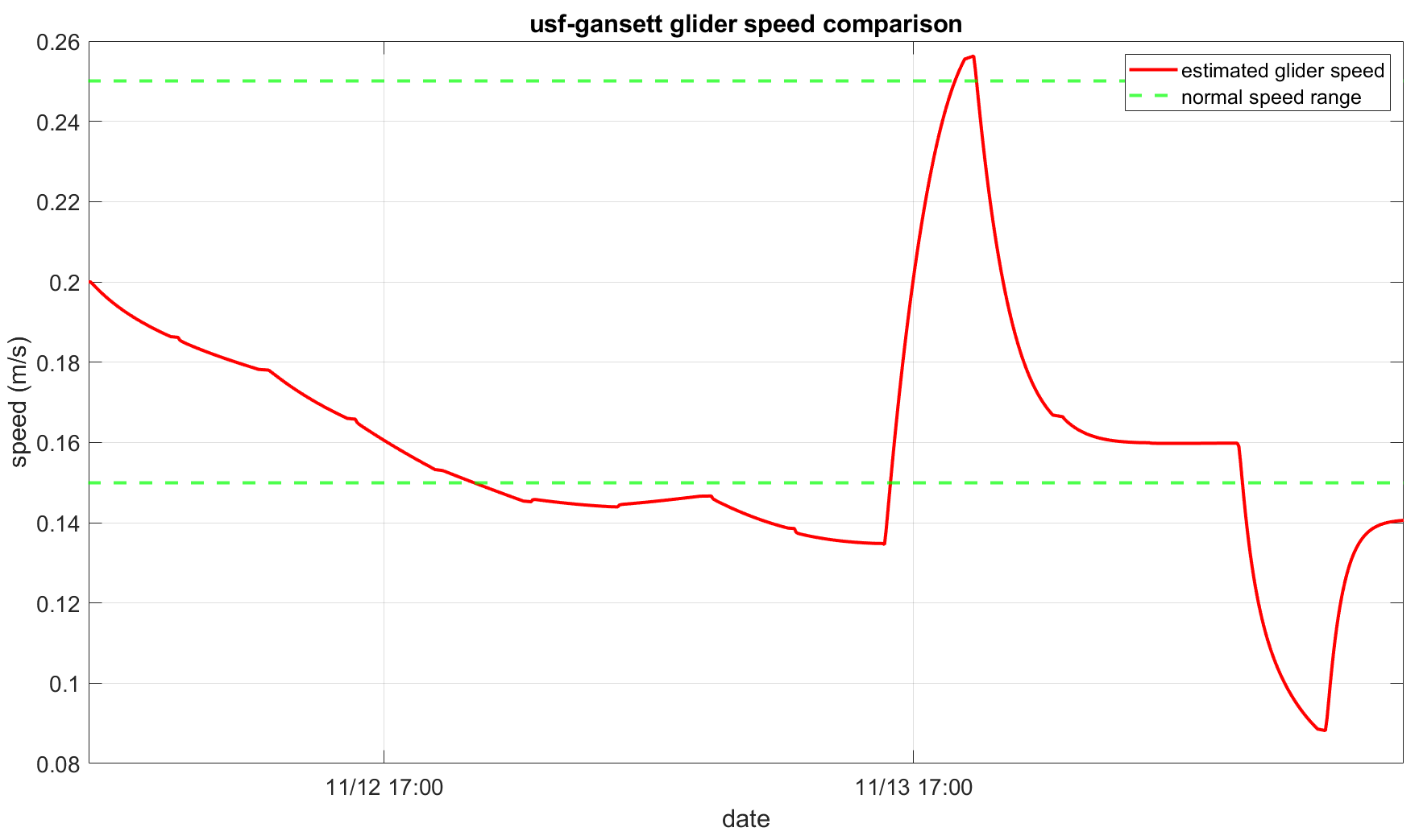
Figure 22: Comparison of estimated glider speed (red) and normal speed range (green) for the 2021 USF-Gansett deployment.

III-B4 USF-Stella

After performing hindcast analysis of the ground truth data as shown in Fig. 23, the glider team was certain that USF-Stella takes several hits during the deployment. At some point, the strike was serious enough that one of the wing support rails are broken, as shown in Fig. 24.

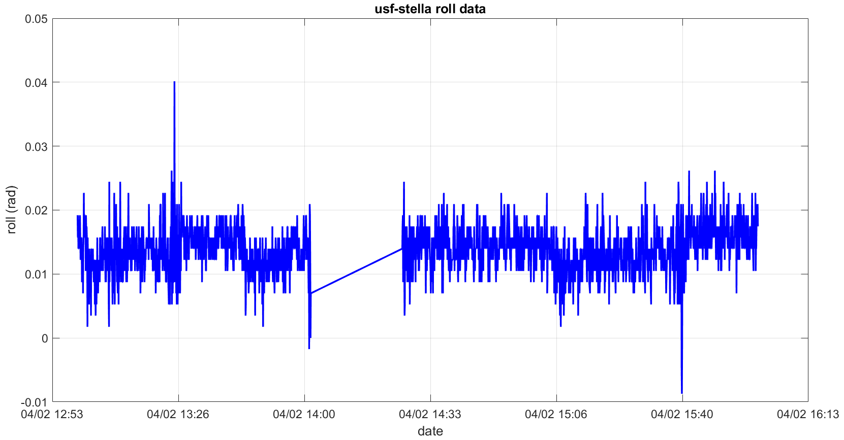
(a) Glider-measured roll (rad) from post-recovery DBD data.

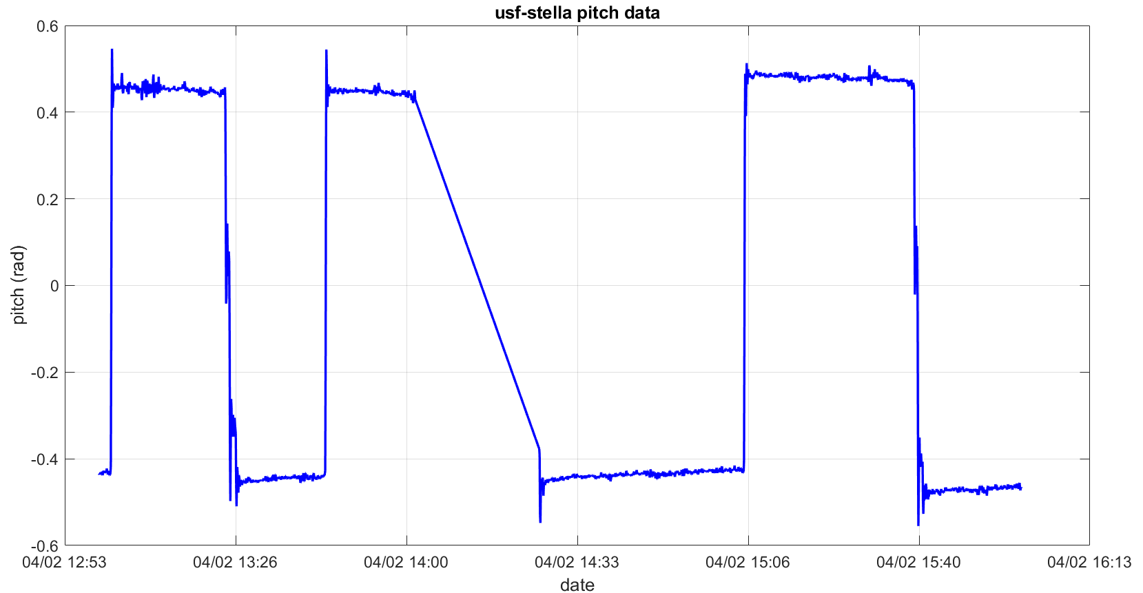
(b) Glider-measured pitch (rad) from post-recovery DBD data.

Figure 23: ground truth for the 2023 USF-Stella deployment.

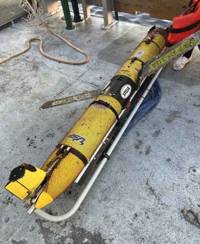
Figure 24: Broken support rails of USF-Stella.

Based on the DBD data, the algorithm-estimated trajectory is close to the true trajectory, as shown in Fig. 25. From quantitative analysis in Fig. 26, the maximum CLLE $45m$ is small enough to conclude the CLLE convergence. We follow the same process of evaluating flow estimation error in Section III-B1. As shown in Fig. 27, the small flow estimation error suggests that the detection result can be trusted. As shown in Fig. 28, the estimated glider speed dropped out of the normal speed range (green dot line) at around April 02, 2023, 15:00 UTC. The anomaly timestamp detected by the algorithm corresponds to the timestamp in the glider team’s report.

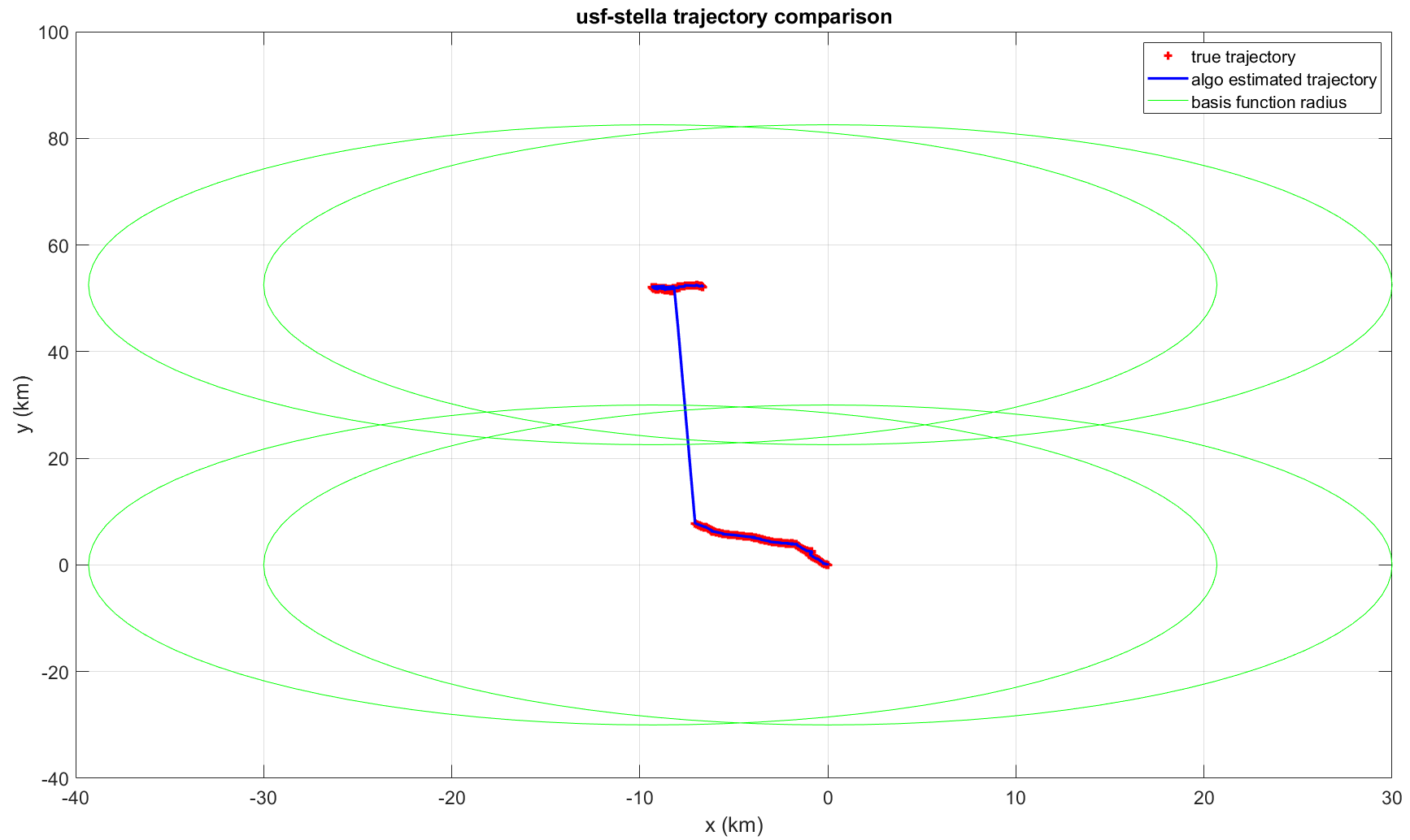
Figure 25: Comparison of the estimated (blue) and true (red) trajectory for the 2023 USF-Stella deployment. The four green circles are the four basis functions covering the whole trajectory.

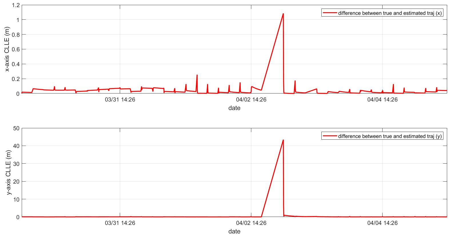
Figure 26: CLLE (m) for the 2023 USF-Stella deployment.

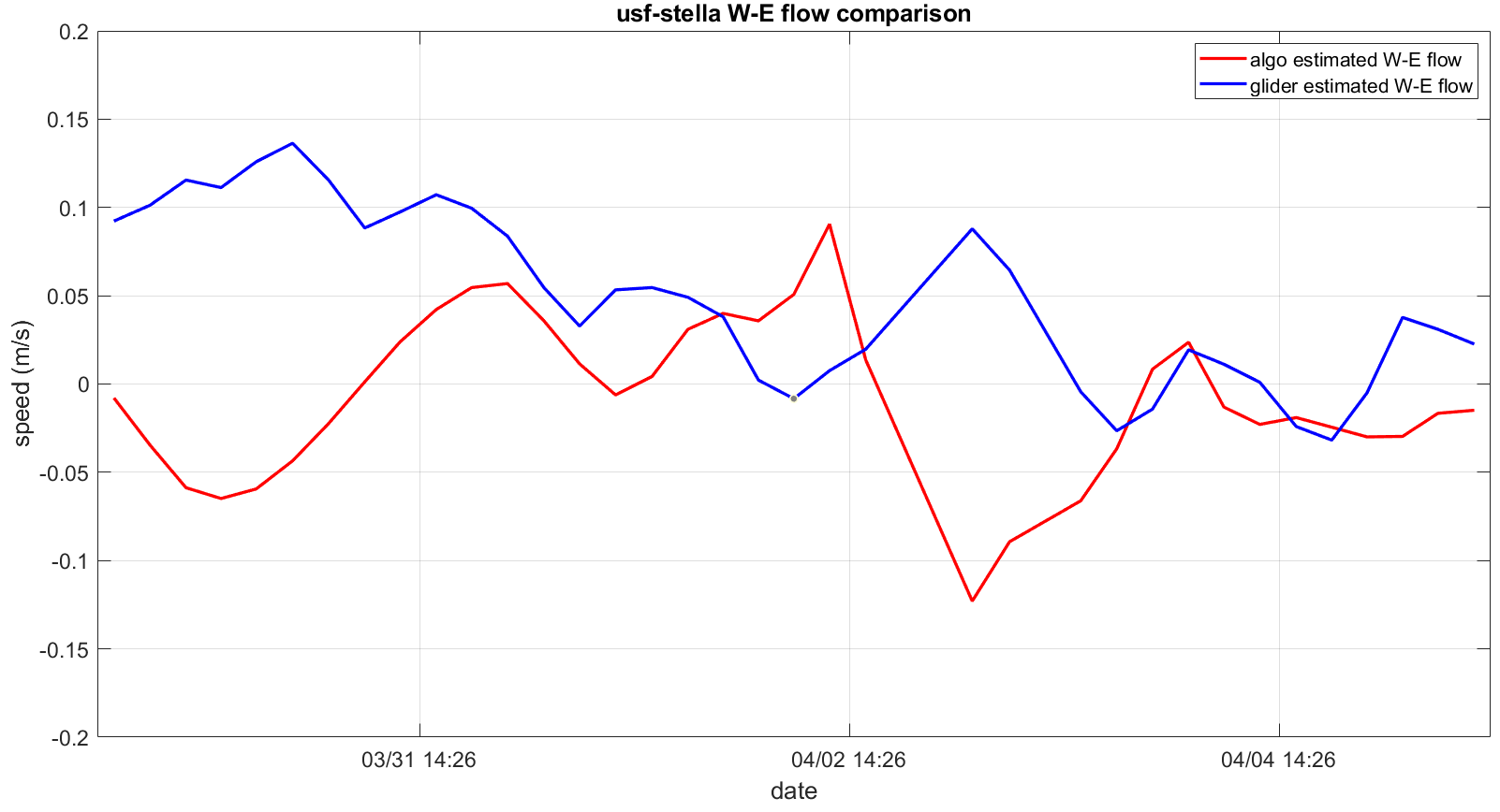
(a) W-E flow component.

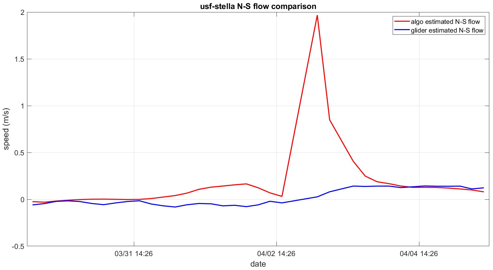
(b) N-S flow component.

Figure 27: Comparison of glider-estimated and algorithm-estimated W-E ($u$, upper) and N-S ($v$, lower) flow velocities for the 2023 USF-Stella deployment.

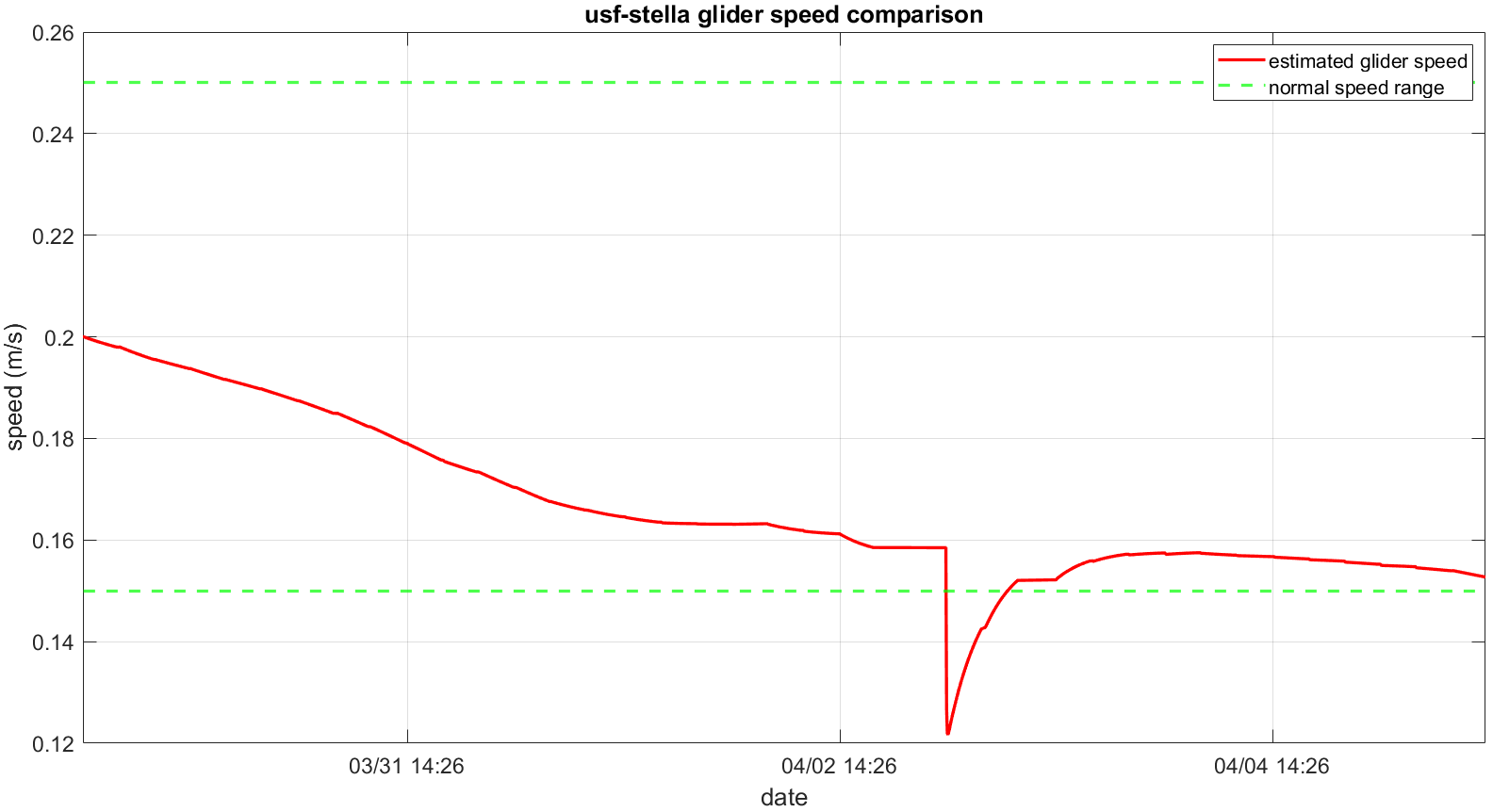
Figure 28: Comparison of estimated glider speed (red) and normal speed range (green) for the 2023 USF-Stella deployment.

IV Conclusion

In this paper, we apply an anomaly detection algorithm to four real glider missions supported by the Skidaway Institute of Oceanography in the University of Georgia and the University of South Florida. On one side of generality, the algorithm is capable of detecting anomalies like remora attachment and shark hit in diverse real-world deployments based on high-resolution DBD data. On the other side of real-time performance, we simulate the online detection on subsetted SBD data. It utilizes generic data of glider trajectory and heading angle to estimate glider speed and flow speed. Anomalies can be identified by comparing the estimated glider speed with the normal speed range. False alarms can be minimized by comparing the algorithm-estimated flow speed with the glider-estimated flow speed. The algorithm achieves real-time estimation through a model-based framework by continuously updating estimates based on ongoing deployment feedback. Future work will enhance estimation accuracy by incorporating large amount of glider data into a data-driven framework. It is also worth taking into account the impact of the anomaly on the estimated flow speed, aiding in the process of determining false alarms.

References

- [1] F. Zhang, D. M. Fratantoni, D. A. Paley, J. M. Lund, and N. E. Leonard, “Control of coordinated patterns for ocean sampling,” International Journal of Control, vol. 80, no. 7, pp. 1186–1199, 2007.
- [2] D. A. Paley, F. Zhang, and N. E. Leonard, “Cooperative control for ocean sampling: The glider coordinated control system,” IEEE Transactions on Control Systems Technology, vol. 16, no. 4, pp. 735–744, 2008.
- [3] M. Hou, S. Cho, H. Zhou, C. R. Edwards, and F. Zhang, “Bounded cost path planning for underwater vehicles assisted by a time-invariant partitioned flow field model,” Frontiers in Robotics and AI, vol. 8, 2021.
- [4] J. Nicholson and A. Healey, “The present state of autonomous underwater vehicle (auv) applications and technologies,” Marine Technology Society Journal, vol. 42, no. 1, pp. 44–51, 2008.
- [5] O. Schofield, J. Kohut, D. Aragon, L. Creed, J. Graver, C. Haldeman, J. Kerfoot, H. Roarty, C. Jones, D. Webb et al., “Slocum gliders: Robust and ready,” Journal of Field Robotics, vol. 24, no. 6, pp. 473–485, 2007.
- [6] M. J. Stanway, B. Kieft, T. Hoover, B. Hobson, D. Klimov, J. Erickson, B. Y. Raanan, D. A. Ebert, and J. Bellingham, “White shark strike on a long-range auv in monterey bay,” in OCEANS 2015-Genova. IEEE, 2015, pp. 1–7.
- [7] J. E. McCosker and R. N. Lea, “White shark attacks upon humans in california and oregon, 1993-2003,” Proceedings-California Academy Of Sciences, vol. 57, no. 12/24, p. 479, 2006.
- [8] L. G. Baehr, “Swimming with sharks: An underwater robot learns how to track great whites,” Oceanus, vol. 50, no. 2, pp. 42–49, 2013.
- [9] J. J. Gertler, Fault detection and diagnosis in engineering systems. CRC press, 2017.
- [10] J. Chen and R. J. Patton, Robust model-based fault diagnosis for dynamic systems. Springer Science & Business Media, 2012, vol. 3.
- [11] K. Aslansefat, G. Latif-Shabgahi, and M. Kamarlouei, “A strategy for reliability evaluation and fault diagnosis of autonomous underwater gliding robot based on its fault tree,” International Journal of Advances in Science Engineering and Technology, vol. 2, no. 4, pp. 83–89, 2014.
- [12] X. Wang, “Active fault tolerant control for unmanned underwater vehicle with sensor faults,” IEEE Transactions on Instrumentation and Measurement, vol. 69, no. 12, pp. 9485–9495, 2020.
- [13] B. Y. Raanan, J. Bellingham, Y. Zhang, B. Kieft, M. J. Stanway, R. McEwen, and B. Hobson, “A real-time vertical plane flight anomaly detection system for a long range autonomous underwater vehicle,” in OCEANS 2015 - MTS/IEEE Washington, 2015, pp. 1–6.
- [14] E. Anderlini, C. A. Harris, G. Salavasidis, A. Lorenzo, A. B. Phillips, and G. Thomas, “Autonomous detection of the loss of a wing for underwater gliders,” in 2020 IEEE/OES Autonomous Underwater Vehicles Symposium (AUV). IEEE, 2020, pp. 1–6.
- [15] G. Fagogenis, V. De Carolis, and D. M. Lane, “Online fault detection and model adaptation for underwater vehicles in the case of thruster failures,” in 2016 IEEE International Conference on Robotics and Automation (ICRA). IEEE, 2016, pp. 2625–2630.
- [16] Y.-s. Sun, X.-r. Ran, Y.-m. Li, G.-c. Zhang, and Y.-h. Zhang, “Thruster fault diagnosis method based on gaussian particle filter for autonomous underwater vehicles,” International Journal of Naval Architecture and Ocean Engineering, vol. 8, no. 3, pp. 243–251, 2016.
- [17] A. Caiti, F. Di Corato, F. Fabiani, D. Fenucci, S. Grechi, and F. Pacini, “Enhancing autonomy: Fault detection, identification and optimal reaction for over—actuated auvs,” in OCEANS 2015-Genova. IEEE, 2015, pp. 1–6.
- [18] V. Asalapuram, I. Khan, and K. Rao, “A novel architecture for condition based machinery health monitoring on marine vessels using deep learning and edge computing,” in 2019 IEEE International Symposium on Measurement and Control in Robotics (ISMCR). IEEE, 2019, pp. C1–3.
- [19] P. Wu, C. A. Harris, G. Salavasidis, I. Kamarudzaman, A. B. Phillips, G. Thomas, and E. Anderlini, “Anomaly detection and fault diagnostics for underwater gliders using deep learning,” in OCEANS 2021: San Diego–Porto. IEEE, 2021, pp. 1–6.
- [20] Z. Bedja-Johnson, P. Wu, D. Grande, and E. Anderlini, “Smart anomaly detection for slocum underwater gliders with a variational autoencoder with long short-term memory networks,” Applied Ocean Research, vol. 120, p. 103030, 2022.
- [21] V. Chandola, A. Banerjee, and V. Kumar, “Anomaly detection: A survey,” ACM computing surveys (CSUR), vol. 41, no. 3, pp. 1–58, 2009.
- [22] W. Yassin, N. I. Udzir, Z. Muda, and M. N. Sulaiman, “Anomaly-based intrusion detection through k-means clustering and naives bayes classification,” International Conference on Computing and Informatics, p. 49, 2013.
- [23] K. Szwaykowska and F. Zhang, “Controlled lagrangian particle tracking: error growth under feedback control,” IEEE Transactions on Control Systems Technology, vol. 26, no. 3, pp. 874–889, 2017.
- [24] S. Cho, F. Zhang, and C. R. Edwards, “Learning and detecting abnormal speed of marine robots,” International Journal of Advanced Robotic Systems, vol. 18, no. 2, p. 1729881421999268, 2021.
- [25] R. Yang, M. Hou, C. Lembke, C. Edwards, and F. Zhang, “Anomaly detection of underwater gliders verified by deployment data,” in 2023 IEEE Underwater Technology (UT). IEEE, 2023, pp. 1–10.
- [26] Y. Ruochu, M. Hou, C. Lembke, C. Edwards, and F. Zhang, “Real-time autonomous glider navigation software,” arXiv preprint arXiv:2304.13096, 2023.
- [27] X. Liang, W. Wu, D. Chang, and F. Zhang, “Real-time modelling of tidal current for navigating underwater glider sensing networks,” Procedia Computer Science, vol. 10, pp. 1121–1126, 2012.
- [28] O. Schofield, J. Kohut, D. Aragon, L. Creed, J. Graver, C. Haldeman, J. Kerfoot, H. Roarty, C. Jones, D. Webb, and S. Glenn, “Slocum gliders: Robust and ready,” Journal of Field Robotics, vol. 24, no. 6, pp. 473–485, 2007.