Geometric ergodicity of trans-dimensional Markov chain Monte Carlo algorithms

Abstract

This article studies the convergence properties of trans-dimensional MCMC algorithms when the total number of models is finite. It is shown that, for reversible and some non-reversible trans-dimensional Markov chains, under mild conditions, geometric convergence is guaranteed if the Markov chains associated with the within-model moves are geometrically ergodic. This result is proved in an $L^{2}$ framework using the technique of Markov chain decomposition. While the technique was previously developed for reversible chains, this work extends it to the point that it can be applied to some commonly used non-reversible chains. Under geometric convergence, a central limit theorem holds for ergodic averages, even in the absence of Harris ergodicity. This allows for the construction of simultaneous confidence intervals for features of the target distribution. This procedure is rigorously examined in a trans-dimensional setting, and special attention is given to the case where the asymptotic covariance matrix in the central limit theorem is singular. The theory and methodology herein are applied to reversible jump algorithms for two Bayesian models: an autoregression with Laplace errors and unknown model order, and a probit regression with variable selection.

1 Introduction

In many statistical setups, the parameter space of interest is a union of disjoint subsets, where each subset corresponds to a model, and the dimensions of the subsets need not be the same. Trans-dimensional Markov chain Monte Carlo (MCMC) is a class of algorithms for sampling from distributions defined on such spaces, which allows for model selection as well as parameter estimation. This type of algorithms, especially the reversible jump MCMC developed by Green (1995), have been applied to important problems like change-point estimation (Green, 1995), autoregression models (Troughton and Godsill, 1998; Ehlers and Brooks, 2002; Vermaak et al., 2004), variable selection (Chevallier et al., 2022), wavelet models (Cornish and Littenberg, 2015) etc. The current article aims to provide conditions on geometric ergodicity for trans-dimensional Markov chains when the total number of models is finite.

Let $\mathcal{K}$ be a finite set whose elements are referred to as “models.” A model $k$ in $\mathcal{K}$ is associated with a non-empty measurable space $(\mathsf{Z}_{k},\mathcal{A}_{k})$ and a nonzero finite measure $\Psi_{k}$ on $(\mathsf{Z}_{k},\mathcal{A}_{k})$. Let $\mathsf{X}=\bigcup_{k\in\mathcal{K}}\{k\}\times\mathsf{Z}_{k}$, and let $\mathcal{B}$ be the sigma algebra generated by sets of the form $\{k\}\times A$, where $k\in\mathcal{K}$ and $A\in\mathcal{A}_{k}$. Consider the task of sampling from the probability measure $\Pi$ on $(\mathsf{X},\mathcal{B})$ such that

$$\Pi(\{k\}\times A)=\frac{\Psi_{k}(A)}{\sum_{k^{\prime}\in\mathcal{K}}\Psi_{k^{\prime}}(\mathsf{Z}_{k^{\prime}})},\quad k\in\mathcal{K},\;A\in\mathcal{A}_{k}.$$ (1)

Suppose that a procedure generates a random element $(K,Z)\sim\Pi$. Then, for $k\in\mathcal{K}$, $\Psi_{k}(\mathsf{Z}_{k})/\sum_{k^{\prime}\in\mathcal{K}}\Psi_{k^{\prime}}(\mathsf{Z}_{k^{\prime}})$ gives the probability of $K=k$, and $\Phi_{k}(\cdot)=\Psi_{k}(\cdot)/\Psi_{k}(\mathsf{Z}_{k})$ gives the conditional distribution of $Z$ given $K=k$.

In practice, $\Pi$ is often intractable, prompting the use of trans-dimensional MCMC methods. A central goal of the current work is to provide verifiable sufficient conditions for trans-dimensional MCMC algorithms to be geometrically convergent in the $L^{2}$ distance. When $\mathcal{B}$ is countably generated and the Markov chain is $\varphi$-irreducible, $L^{2}$ geometric convergence implies the classical notion of $\Pi$-a.e. geometric ergdoicity. See Lemma 4 in Section 2, which is taken from Roberts and Rosenthal (1997), Roberts and Tweedie (2001), and Gallegos-Herrada et al. (2023). As discussed in Section 5, geometric ergodicity guarantees a central limit theorem (CLT) for ergodic sums; moreover, consistent estimation of the asymptotic variance in a CLT often relies on geometric ergodicity.

The convergence behavior of trans-dimensional MCMC algorithms is in general far from well understood. Roberts and Rosenthal (2006) established some general conditions for trans-dimensional Markov chains to be Harris recurrent. Geometric ergodicity of some specific trans-dimensional algorithms was established in Geyer and Møller (1994), Andrieu and Doucet (1999), Ortner et al. (2006), and Schreck et al. (2015). Existing proofs of geometric ergodicity often rely on the technique of drift and minorization, or in some simple situations, Doeblin’s condition. The current work instead utilizes the decomposition of Markov chains, a remarkable technique developed by Caracciolo et al. (1992) and documented in Madras and Randall (2002). This technique allows one to decompose the dynamic of a trans-dimensional Markov chain into within- and between-model movements, which can be analyzed separately. Using an extended version of this technique and exploiting the assumption that $|\mathcal{K}|<\infty$, Theorem 1 is established. This result describes a divide-and-conquer paradigm that enables one to establish geometric convergence of the trans-dimensional chain by combining the geometric ergodicity of its within-model components. A quantitative bound on the convergence rate will also be provided; see Theorem 8.

Previously, Markov chain decomposition has found its use in important problems like simulated and parallel tempering. See, e.g., Madras and Randall (2002); Ge et al. (2018); Woodard et al. (2009). Loosely speaking, this technique can be used to analyze a Markov chain whose state space can be partitioned into subsets such that, within each subset, the Markov chain’s behavior is easy to analyze. It was originally developed for reversible Markov chains, especially those with positive semi-definite Markov operators. The current work provides an extended version of the technique, given in Lemma 6, that can deal with some important non-reversible chains.

While $L^{2}$ geometric convergence guarantees geometric ergodicity in an almost sure sense, it does not ensure Harris ergodicity, i.e., Harris recurrence in addition to aperirodicity and $\varphi$-irreducibility. Many theoretical results for Markov chain samples, such as the law of large numbers and the central limit theorem, are typically stated when assuming Harris ergodicity. Roberts and Rosenthal (2006) provided some useful conditions that lead to Harris recurrence in trans-dimensional settings. However, these conditions could be tricky to verify in practice. In Lemma 9, it is shown that $\Pi$-a.e. geometric convergence is, in a broad sense, as good as Harris ergodicity, so long as the chain’s starting distribution is absolutely continuous with respect to $\Pi$.

This article also discusses how geometric convergence allows for uncertainty quantification in Monte Carlo estimation in trans-dimensional settings. In particular, it studies the construction of simultaneous confidence intervals based on a Monte Carlo sample. The study is based on a method developed by Robertson et al. (2020) along with works on Markov chain CLT and asymptotic variance estimation. A key challenge in trans-dimensional settings is that the asymptotic covariance matrix of a vector-valued Monte Carlo estimator is typically singular. This makes existing methods difficult to apply or justify. To circumvent the problem, a small amount of random noise is injected into the Monte Carlo estimator to turn the asymptotic covariance matrix non-singular. This results in simultaneous confidence intervals that are theoretically correct and practically stable.

The theory developed herein is applied to reversible jump MCMC algorithms for two practical Bayesian models: an autoregressive model with Laplace errors and unknown model order, and a probit regression model with variable selection. For each algorithm, we establish geometric convergence, and assess the Monte Carlo errors through the construction of simultaneous confidence intervals.

This work focuses on the case where the number of models is finite. Many model selection problems fall into this category (see, e.g., Green, 1995; Troughton and Godsill, 1998; Chevallier et al., 2022), although problems like spatial point processes do not.

Finally, it must be emphasized that verifying geometric ergodicity is but one of the first steps towards fully understanding the convergence behavior of an MCMC algorithm. A chain being geometrically convergent does not ensure that it has a fast convergence rate. While this work does provide a quantitative convergence rate bound, calculating the quantities involved in the bound can be practically challenging. Obtaining sharp estimates for the convergence rate remains an open problem for most practical trans-dimensional MCMC algorithms.

The rest of this article is organized as follows. Following a quick overview of the main qualitative result of this article, Section 2 contains some preliminary facts on the $L^{2}$ theory of Markov chains. The main technical results involving Markov chain decomposition and the convergence rate of trans-dimensional MCMC are given in Section 3. Section 4 contains a discussion on the implications of almost everywhere ergodicity. Section 5 studies the problem of uncertainty quantification in trans-dimensional Monte Carlo simulation. Two practical examples are studied in Section 6. The Appendices contain some technical proofs. The code for the computer experiments in Section 6 is collected in a supplementary file.

1.1 Conditions for geometric ergodicity: An overview

Consider a trans-dimensional Markov chain $(X(t))_{t=0}^{\infty}=(K(t),Z(t))_{t=0}^{\infty}$ whose state space is $\mathsf{X}$. Let $P$ be its Markov transition kernel (Mtk). Suppose that $\Pi$ is a stationary distribution of this chain, i.e., $\Pi=\Pi P$, or more explicitly, for $\bigcup_{k\in\mathcal{K}}\{k\}\times A_{k}\in\mathcal{B}$,

$$\sum_{k^{\prime}\in\mathcal{K}}\Psi_{k^{\prime}}(A_{k^{\prime}})=\sum_{k\in\mathcal{K}}\sum_{k^{\prime}\in\mathcal{K}}\int_{\mathsf{Z}_{k}}\Psi_{k}(\mathrm{d}z)P((k,z),\{k^{\prime}\}\times A_{k^{\prime}}).$$

Let us decompose the chain’s dynamic into within- and between-model movements.

Given $k\in\mathcal{K}$, $(z,A)\mapsto P((k,z),\{k\}\times A)$ describes how the chain moves within the model, i.e., inside $\{k\}\times\mathsf{Z}_{k}$. To outline the between-model jumps, consider, for $(k,k^{\prime})\in\mathcal{K}\times\mathcal{K}$, whether a move from model $k$ to model $k^{\prime}$ is possible. To be specific, let $\gamma_{k,k^{\prime}}=1$ if

$$\int_{\mathsf{Z}_{k}}\Psi_{k}(\mathrm{d}z)P((k,z),\{k^{\prime}\}\times\mathsf{Z}_{k^{\prime}})>0,$$

and $\gamma_{k,k^{\prime}}=0$ otherwise. List the elements of $\mathcal{K}$ in an arbitrary order, say, $k_{(1)},k_{(2)},\dots,k_{(|\mathcal{K}|)}$. Let $\Gamma_{P}$ be the $|\mathcal{K}|\times|\mathcal{K}|$ matrix whose $i,j$th element is $\gamma_{k_{(i)},k_{(j)}}$ for $i,j\in\{1,\dots,|\mathcal{K}|\}$.

The main result of this paper is stated in terms the $L^{2}$ theory for Markov chains, which is reviewed in Section 2. Essentially, if $T$ is an Mtk that has a stationary distribution $\omega$, then $T$ can be regarded as a bounded linear operator on a certain Hilbert space $L_{0}^{2}(\omega)$. A sufficient condition for the corresponding chain to be $L^{2}$ geometrically convergent is that the operator norm of some power of $T$ is less than one.

One of the main results of this paper is stated below. See Section 3 for more details.

Theorem 1.

Assume that each of the following conditions holds for the trans-dimensional chain:

1. For $k\in\mathcal{K}$, there is an Mtk $P_{k}:\mathsf{Z}_{k}\times\mathcal{A}_{k}\to[0,1]$ that has the following properties:

   1. $\Phi_{k}P_{k}=\Phi_{k}$, where $\Phi_{k}(\cdot)=\Psi_{k}(\cdot)/\Psi_{k}(\mathsf{Z}_{k})$ is the normalization of $\Psi_{k}(\cdot)$.

   2. When $P_{k}$ is regarded as an operator on $L_{0}^{2}(\Phi_{k})$, the norm of its $t$th power $P_{k}^{t}$ is strictly less than one for some positive integer $t$.

   3. there exists a constant $c_{k}>0$ such that

      $$P((k,z),\{k\}\times A)\geq c_{k}P_{k}(z,A)$$

      for $z\in\mathsf{Z}_{k}$ and $A\in\mathcal{A}_{k}$.

2. For some positive integer $s$, each element in the matrix $\Gamma_{P}^{s}$ is positive.

Then the norm of $P^{t}$ is strictly less than one, and the trans-dimensional chain is $L^{2}(\Pi)$ geometrically convergent.

In practice, $\Gamma_{P}$ is usually straightforward to compute, and it would not be difficult to verify (H2), which is evidently very mild. The following lemma, which is proved in Appendix A, provides another way to establish (H2) using the chain’s $s$-step transition kernel $P^{s}(\cdot,\cdot)$.

Lemma 2.

Let $s$ be a positive integer. Suppose that, for $k,k^{\prime}\in\mathcal{K}$,

$$\int_{\mathsf{Z}_{k}}\Psi_{k}(\mathrm{d}z)P^{s}((k,z),\{k^{\prime}\}\times\mathsf{Z}_{k^{\prime}})>0,$$

i.e., if $z$ is distributed as $\Psi_{k}$, then a chain starting from $(k,z)$ is capable of reaching $\{k^{\prime}\}\times\mathsf{Z}_{k^{\prime}}$ after exactly $s$ iterations. Then each element of $\Gamma_{P}^{s}$ is positive.

Trans-dimensional MCMC algorithms typically involve a within-model move type, where the underlying chain stays in a model, say $k$, with probability $c_{k}$, and move according to an Mtk $P_{k}$ such that $\Phi_{k}P_{k}=\Phi_{k}$. Then such $c_{k}$ and $P_{k}$ satisfy (i) and (iii) in (H1). Condition (ii) in (H1) requires a careful analysis of the within-model moves of an algorithm. According to Lemma 3 below, in several important situations, this condition is implied by the geometric ergodicity of the chain associated with $P_{k}$, or some closely related Markov chain whose state space is $\mathsf{Z}_{k}$. Since the space $\mathsf{Z}_{k}$ is typically of a fixed dimension, the hope is that chains that move in $\mathsf{Z}_{k}$ can be analyzed using well-established tools such as drift and minorization or functional inequalities.

Lemma 3.

Let $k$ be in $\mathcal{K}$. Suppose that $\mathcal{B}_{k}$ is countably generated, $\Phi_{k}P_{k}=\Phi_{k}$, and the chain associated with $P_{k}$ is $\varphi$-irreducible. Then, in each of the following situations, (ii) in (H1) holds with $t=1$.

1. $P_{k}$ defines a $\Phi_{k}$-a.e. geometrically ergodic chain that is reversible with respect to $\Phi_{k}$.

2. $P_{k}$ defines a deterministic-scan Gibbs chain with two components that is $\Phi_{k}$-a.e. geometrically ergodic.

3. $P_{k}$ defines a deterministic-scan Gibbs chain, and there exists a $\Phi_{k}$-a.e. geometrically ergodic random-scan Gibbs chain based on the same set of conditional distributions.

Proof.

For (i), see Theorem 2.1 of Roberts and Rosenthal (1997) and Theorem 2 of Roberts and Tweedie (2001). For (ii), see Lemma 3.2 and Proposition 3.5 of Qin and Jones (2022). For (iii), see Theorem 3.1 of Chlebicka et al. (2023) and invoke (i). ∎

2 Preliminaries

Let $(\mathsf{Y},\mathcal{F},\omega)$ be a generic probability space. Let $L^{2}(\omega)$ be the space of real functions $f:\mathsf{Y}\to\mathbb{R}$ that are square integrable with respect to $\omega$. Two functions in $L^{2}(\omega)$ are regarded as identical if they are almost everywhere equal. For $f,g\in L^{2}(\omega)$, define their inner-product

$$\langle f,g\rangle_{\omega}=\int_{\mathsf{Y}}f(y)g(y)\,\omega(\mathrm{d}y),$$

and let $\|f\|_{\omega}=\sqrt{\langle f,f\rangle_{\omega}}$. Then $(L^{2}(\omega),\langle\cdot,\cdot\rangle)$ forms a Hilbert space. Denote by $L_{0}^{2}(\omega)$ the subspace of $L^{2}(\omega)$ that consists of functions $f$ such that $\omega f:=\langle f,\mathbf{1}_{\mathsf{Y}}\rangle_{\omega}=0$, where $\mathbf{1}_{\mathsf{Y}}(y)=1$ for $y\in\mathsf{Y}$. A probability measure $\mu$ on $(\mathsf{Y},\mathcal{F})$ is said to be in $L_{*}^{2}(\omega)$ if $\mathrm{d}\mu/\mathrm{d}\omega$ exists and is in $L^{2}(\omega)$. For two probability measures $\mu$ and $\nu$ in $L_{*}^{2}(\omega)$, define their $L^{2}$ distance by

$$\|\mu-\nu\|_{\omega}=\sup_{f\in L^{2}(\omega),\,\|f\|_{\omega}=1}|\mu f-\nu f|=\left\|\frac{\mathrm{d}\mu}{\mathrm{d}\omega}-\frac{\mathrm{d}\nu}{\mathrm{d}\omega}\right\|_{\omega}.$$

Let $T:\mathsf{Y}\times\mathcal{F}\to[0,1]$ be an Mtk whose stationary distribution is $\omega$. Assume that $T$ is associated with a Markov chain $(Y(t))_{t=0}^{\infty}$. For a non-negative integer $t$, the power $T^{t}$ denotes the $t$-step transition kernel, so that $T^{0}(y,\cdot)$ is the Dirac measure (point mass) at a point $y\in\mathsf{Y}$, $T^{1}=T$, and $T^{t+1}(y,\cdot)=\int_{\mathsf{Y}}T^{t}(y,\mathrm{d}y^{\prime})T(y^{\prime},\cdot)$. Then, for a probability measure $\mu$ on $\mathcal{F}$, $\mu T^{t}(\cdot):=\int_{\mathsf{Y}}\mu(\mathrm{d}y)T^{t}(y,\cdot)$ gives the marginal distribution $Y(t)$ if $Y(0)\sim\mu$. We say that the chain $Y(t)$ or the Mtk $T$ is $L^{2}(\omega)$ geometrically convergent if there exist $\rho<1$ and a function $C:L_{*}^{2}(\omega)\to[0,\infty)$ such that for $\mu\in L_{*}^{2}(\omega)$ and $t\geq 0$,

$$\|\mu T^{t}-\omega\|_{\omega}\leq C(\mu)\rho^{t}.$$ (2)

A closely related concept is geometric ergodicity. Let $\|\cdot\|_{\scriptsize\mbox{TV}}$ be the total variance distance, and let $\delta_{y}$ denote the Dirac measure at a point $y\in\mathsf{Y}$. The chain $Y(t)$ (or the Mtk $T$) is $\omega$-a.e. geometrically ergodic if there exist $\rho<1$ and $C:\mathsf{Y}\to[0,\infty)$ such that $\omega C<\infty$, and that, for $\omega$-almost every $y\in\mathsf{Y}$ and $t\geq 0$,

$$\|\delta_{y}T^{t}-\omega\|_{\scriptsize\mbox{TV}}\leq C(y)\rho^{t}.$$ (3)

In the literature, the term “geometric ergodicity” often means $\omega$-a.e. geometric ergodicity in addition to Harris ergodicity.

The following result is from Roberts and Tweedie (2001) with slight modifications; see also Roberts and Rosenthal (1997) and Gallegos-Herrada et al. (2023).

Lemma 4.

Suppose that $\mathcal{F}$ is countably generated and that $Y(t)$ is $\varphi$-irreducible. Then the following two statements are true.

1. If the chain is $L^{2}(\omega)$ geometrically convergent, then it is $\omega$-a.e. geometrically ergodic.

2. If the chain is reversible with respect to $\omega$, then it is $L^{2}(\omega)$ geometrically convergent if and only if it is $\omega$-a.e. geometrically ergodic.

Proof.

This is essentially Theorems 1 and 2 of Roberts and Tweedie (2001). The only difference is that in Roberts and Tweedie (2001), $\omega$-a.e. geometric ergodicity is defined without assuming that $\omega C<\infty$ in (3), so (i) still needs some explanation. In the proof of Theorem 1 of Roberts and Tweedie (2001), it is argued that a $\varphi$-irreducible and $L^{2}(\omega)$ geometrically ergodic chain must be aperiodic. Then, by Proposition 2.1 of Roberts and Rosenthal (1997), if (3) holds $\omega$-a.e. for some $\rho<1$ and finite $C(y)$, then one can find some $\rho_{1}<1$ and finite $C_{1}(y)$ such that $\omega C_{1}<\infty$ for which (3) holds $\omega$-a.e.. ∎

The Mtk $T$ can be understood as a linear operator on $L_{0}^{2}(\omega)$: for $f\in L_{0}^{2}(\omega)$,

$$Tf(\cdot)=\int_{\mathsf{Y}}T(\cdot,\mathrm{d}y)f(y).$$

The $t$th power of the operator $T$ corresponds precisely to the $t$-step mtk $T^{t}$. One can use the Cauchy-Schwarz inequality to show that

$$\|T\|_{\omega}:=\sup_{f\in L_{0}^{2}(\omega)\setminus\{0\}}\frac{\|Tf\|_{\omega}}{\|f\|_{\omega}}\leq 1.$$

The following is well-known. See, e.g, Theorem 2.1 of Roberts and Rosenthal (1997).

Lemma 5.

Let $s$ be an arbitrary positive integer. If $\|T^{s}\|_{\omega}>0$, then equation (2) holds for all $\mu\in L_{*}^{2}(\omega)$ and $t\geq 0$ with $\rho=\|T^{s}\|_{\omega}^{1/s}$ and some $C(\cdot)$. If $\|T^{s}\|_{\omega}=0$, then equation (2) holds for all $\mu\in L_{*}^{2}(\omega)$ and $t\geq 0$ with an arbitrary $\rho>0$ and some $C(\cdot)$. If the chain is reversible, then there exists some $C(\cdot)$ such that (2) holds for all $\mu\in L_{*}^{2}(\omega)$ and $t\geq 0$ if and only if $\rho\geq\|T\|_{\omega}=\|T^{s}\|_{\omega}^{1/s}$.

The bounded operator $T$ has a unique adjoint $T^{*}$. For $f,g\in L_{0}^{2}(\omega)$, $\langle Tf,g\rangle_{\omega}=\langle f,T^{*}g\rangle_{\omega}$. It is well-known that $\|T\|_{\omega}^{2}=\|T^{*}\|_{\omega}^{2}=\|TT^{*}\|_{\omega}=\|T^{*}T\|_{\omega}$. The chain $(Y(t))$ is reversible if and only if $T=T^{*}$. Finally, $T$ is positive semi-definite if $T=T^{*}$ and $\langle Tf,f\rangle_{\omega}\geq 0$ for $f\in L_{0}^{2}(\omega)$. In this case, $\|T\|_{\omega}$ is the supremum of $\langle f,Tf\rangle_{\omega}/\|f\|_{\omega}^{2}$ when $f$ varies in $L_{0}^{2}(\omega)\setminus\{0\}$.

3 Main Results

3.1 Markov chain decomposition

This subsection describes the main probabilistic tool for proving Theorem 1.

Again, let $(\mathsf{Y},\mathcal{F},\omega)$ be a probability space. Suppose that $\mathsf{Y}$ can be partitioned into a collection of disjoint subsets, $(\mathsf{Y}_{k})_{k\in\mathcal{K}}$. For this subsection, allow $\mathcal{K}$ to be countably infinite. Assume that $\omega(\mathsf{Y}_{k})>0$ for each $k$. Caracciolo et al. (1992) proposed a framework for analyzing a Markov chain moving in $\mathsf{Y}$ by decomposing its dynamic into local movements within a subset $\mathsf{Y}_{k}$ and global movements across the disjoint subsets. The key technical result, published in Madras and Randall (2002), is stated for reversible chains. Here, it is extended to a possibly non-reversible setting.

For $k\in\mathcal{K}$, let $\mathcal{F}_{k}$ be the restriction of $\mathcal{F}$ on $\mathsf{Y}_{k}$, and let $\omega_{k}(B)=\omega(B)/\omega(\mathsf{Y}_{k})$ for $B\in\mathcal{F}_{k}$. For an Mtk $S$ such that $\omega S=\omega$, let $\bar{S}$ be an Mtk on the discrete space $\mathcal{K}$ such that, for $k,k^{\prime}\in\mathcal{K}$,

$$\bar{S}(k,\{k^{\prime}\})=\frac{1}{\omega(\mathsf{Y}_{k})}\int_{\mathsf{Y}}\omega(\mathrm{d}y)S(y,\mathsf{Y}_{k})S(y,\mathsf{Y}_{k^{\prime}}).$$

Let $\bar{\omega}(\{k\})=\omega(\mathsf{Y}_{k})$ for $k\in\mathcal{K}$. Then $\bar{S}$ is reversible with respect to $\bar{\omega}$. In fact, $\bar{S}$ defines a positive semi-definite operator on $L_{0}^{2}(\bar{\omega})$.

Below is the key technical lemma of this subsection, whose proof is given in Appendix B.

Lemma 6.

Let $T$ and $S$ be Mtks such that $\omega T=\omega S=\omega$. Suppose that for $k\in\mathcal{K}$, there exists an Mtk $T_{k}:\mathsf{Y}_{k}\times\mathcal{F}_{k}\to[0,1]$ such that $\omega_{k}T_{k}=\omega_{k}$. Assume further that there exists $c\in[0,1]$ such that $T(y,B)\geq cT_{k}(y,B)$ for $k\in\mathcal{K}$, $y\in\mathsf{Y}_{k}$ and $B\in\mathcal{F}_{k}$. Then

$$1-\|TS^{*}\|_{\omega}^{2}\geq c^{2}\left(1-\sup_{k\in\mathcal{K}}\|T_{k}\|_{\omega_{k}}^{2}\right)(1-\|\bar{S}\|_{\bar{\omega}}).$$ (4)

Intuitively, Lemma 6 relates the norm of $TS^{*}$ to the local behavior of $T$ and the global behavior of $S$. In particular, if $T=S$, then $\|TS^{*}\|_{\omega}=\|TT^{*}\|_{\omega}=\|T\|_{\omega}^{2}$, and this result gives an upper bound on the norm of $T$.

3.2 Geometric convergence of the trans-dimensional chain

Lemma 6 can be used to construct an upper bound on the norm of $P^{t}$ for $t\geq 1$, where $P$ is the Mtk of the trans-dimensional chain defined in the Introduction.

Let $\bar{P}$ be the Mtk on $\mathcal{K}$ such that, for $k,k^{\prime}\in\mathcal{K}$,

$$\bar{P}(k,\{k^{\prime}\})=\frac{1}{\Psi_{k}(\mathsf{Z}_{k})}\sum_{k^{\prime\prime}\in\mathcal{K}}\int_{\mathsf{Z}_{k^{\prime\prime}}}\Psi_{k^{\prime\prime}}(\mathrm{d}z)P((k^{\prime\prime},z),\{k\}\times\mathsf{Z}_{k})P((k^{\prime\prime},z),\{k^{\prime}\}\times\mathsf{Z}_{k^{\prime}}).$$

Let $M_{P}$ be a matrix representation of $\bar{P}$. That is, list the elements of $\mathcal{K}$ in an arbitrary order, say, $k_{(1)},\dots,k_{(|\mathcal{K}|)}$, and let $\bar{P}(k_{(i)},\{k_{(j)}\})$ be the $i,j$th element of $M_{P}$. Since $\bar{P}$ is positive semi-definite, the eigenvalues of $M_{P}$ are all non-negative. Let $\lambda_{1}(M_{P})$ be the second largest eigenvalue of $M_{P}$, taking into account multiplicity. The largest eigenvalue of a Markov transition matrix is always 1, so $\lambda_{1}(M_{P})\leq 1$.

Remark 7.

If $P$ is reversible with respect to $\Pi$, then

$$\bar{P}(k,\{k^{\prime}\})=\int_{\mathsf{Z}_{k}}\Phi_{k}(\mathrm{d}z)P^{2}((k,z),\{k^{\prime}\}\times\mathsf{Z}_{k^{\prime}}).$$

This is an average probability of moving from model $k$ to model $k^{\prime}$ after two steps.

Theorem 8.

Just for this theorem, allow $|\mathcal{K}|$ to be countably infinite. Suppose that condition (H1) in Theorem 1 holds. That is,

1. For $k\in\mathcal{K}$, there is an Mtk $P_{k}:\mathsf{Z}_{k}\times\mathcal{A}_{k}\to[0,1]$ with the following properties: (i) $\Phi_{k}P_{k}=\Phi_{k}$, (ii) $\|P_{k}^{t}\|_{\Phi_{k}}<1$ for some $t\geq 1$, (iii) there exists $c_{k}>0$ such that $P((k,z),\{k\}\times A)\geq c_{k}P_{k}(z,A)$ for $z\in\mathsf{Z}_{k}$ and $A\in\mathcal{A}_{k}$.

Then

$$1-\|P^{t}\|_{\Pi}^{4}\geq\left(\inf_{k\in\mathcal{K}}c_{k}^{t}\right)^{2}\left(1-\sup_{k\in\mathcal{K}}\|P_{k}^{t}\|_{\Phi_{k}}^{2}\right)[1-\lambda_{1}(M_{P})].$$

Proof.

Fix a positive integer $t$. In Lemma 6, take $(\mathsf{Y},\mathcal{F},\omega)=(\mathsf{X},\mathcal{B},\Pi)$, $T=P^{t}$ and $S=P$. For $k\in\mathcal{K}$, let $\mathsf{Y}_{k}=\{k\}\times\mathsf{Z}_{k}$. Then $\mathcal{F}_{k}$ consists of sets of the form $\{k\}\times A$, where $A\in\mathcal{A}_{k}$, and $\omega_{k}(\{k\}\times A)=\Phi_{k}(A)$ for $A\in\mathcal{A}_{k}$. For $k\in\mathcal{K}$, $z\in\mathsf{Z}_{k}$, and $A\in\mathcal{A}_{k}$, let

$$T_{k}((k,z),\{k\}\times A)=P_{k}^{t}(z,A).$$

By (i) in (H1), $\omega_{k}T_{k}=\omega_{k}$. By (iii) in (H1), for $(k,z)\in\mathsf{Y}_{k}$ and $\{k\}\times A\in\mathcal{F}_{k}$,

$$T((k,z),\{k\}\times A)\geq c_{k}^{t}P_{k}^{t}(z,A)\geq cT_{k}((k,z),\{k\}\times A),$$

where $c=\inf_{k\in\mathcal{K}}c_{k}^{t}$. Thus, the assumptions of Lemma 6 are satisfied.

The next step is identifying the objects in (4). Obviously, $\|TS^{*}\|_{\omega}=\|P^{t}P^{*}\|_{\Pi}$. Standard arguments show that $\|T_{k}\|_{\omega_{k}}=\|P_{k}^{t}\|_{\Phi_{k}}$. Since $\bar{S}=\bar{P}$ is positive definite, $\|\bar{S}\|_{\bar{\omega}}$ is the second largest eigenvalue of $M_{P}$. Then, by Lemma 6,

$$1-\|P^{t}P^{*}\|_{\Pi}^{2}\geq c^{2}\left(1-\sup_{k\in\mathcal{K}}\|P_{k}^{t}\|_{\Phi_{k}}^{2}\right)[1-\lambda_{1}(M_{P})].$$

Finally, note that

$$\|P^{t}\|_{\Pi}^{2}=\|P^{t}P^{*t}\|_{\Pi}\leq\|P^{t}P^{*}\|_{\Pi}\|P^{*t-1}\|_{\Pi}=\|P^{t}P^{*}\|_{\Pi}\|P^{t-1}\|_{\Pi}\leq\|P^{t}P^{*}\|_{\Pi}.$$

The desired result then follows. ∎

While some of the quantities in Theorem 8 may be difficult to compute in practice, when $|\mathcal{K}|<\infty$, Theorem 8 immediately yields Theorem 1, which is stated again below:

Theorem 1. Assume that, in addition to (H1), the following condition holds:

1. For some positive integer $s$, each element in the matrix $\Gamma_{P}^{s}$ is positive.

Then $\|P^{t}\|_{\Pi}<1$, and $P$ is $L^{2}(\Pi)$ geometrically convergent.

Proof.

By Theorem 8, it suffices to show that

$$\left(\min_{k\in\mathcal{K}}c_{k}^{t}\right)^{2}\left(1-\max_{k\in\mathcal{K}}\|P_{k}^{t}\|_{\Phi_{k}}^{2}\right)[1-\lambda_{1}(M_{P})]>0.$$

By (iii) in (H1), $\min_{k\in\mathcal{K}}c_{k}^{t}>0$. By (ii) in (H1), $\max_{k\in\mathcal{K}}\|P_{k}^{t}\|_{\Phi_{k}}^{2}<1$. By the definition of $\bar{P}$ and (iii) in (H1), for $(k,k^{\prime})\in\mathcal{K}\times\mathcal{K}$,

$$\Psi_{k}(\mathsf{Z}_{k})\bar{P}(k,\{k^{\prime}\}) \geq\int_{\mathsf{Z}_{k}}\Psi_{k}(\mathrm{d}z)P((k,z),\{k\}\times\mathsf{Z}_{k})P((k,z),\{k^{\prime}\}\times\mathsf{Z}_{k^{\prime}})$$

$$\geq c_{k}\int_{\mathsf{Z}_{k}}\Psi_{k}(\mathrm{d}z)P((k,z),\{k^{\prime}\}\times\mathsf{Z}_{k^{\prime}}).$$

This implies that $\bar{P}(k,\{k^{\prime}\})>0$ whenever $\gamma_{k,k^{\prime}}>0$. It follows that, for a positive integer $s$, an element in $M_{P}^{s}$ is positive whenever the corresponding element in $\Gamma_{P}^{s}$ is positive. Condition (H2) states that all elements of $\Gamma_{P}^{s}$ are positive for some positive integer $s$. This implies that $M_{P}$ defines a irreducible and aperiodic Markov chain on a finite state space. Then this chain must be ergodic, which in turn implies that $\lambda_{1}(M_{P})<1$. The desired result then follows. ∎

The usefulness of Theorem 1 will be demonstrated through two examples in Section 6.

4 Ergodicity Issues

Let $(\mathsf{Y},\mathcal{F},\omega)$ be a generic probability space and suppose that there is an Mtk $T$ such that $\omega=\omega T$. By Lemma 4, when $\mathcal{F}$ is countably generated and the Markov chain associated with $T$ is $\varphi$-irreducible, $L^{2}(\omega)$ geometric convergence implies $\omega$-a.e. geometric ergodicity. Almost everywhere geometric ergodicity does not rule out the possibility of failure to converge from a null set. In particular, it does not guarantee Harris ergodicity, which, when $\mathcal{F}$ is countably generated, is equivalent to $\|\delta_{y}T^{t}-\omega\|_{\scriptsize\mbox{TV}}$ going to 0 as $t\to\infty$ for every $y\in\mathsf{Y}$ (Nummelin, 2004, Proposition 6.3).

Many results in MCMC theory are developed assuming Harris ergodicity. For instance, a standard form of the law of large numbers (LLN) that holds for all initial distributions assumes Harris ergodicity (Meyn and Tweedie, 2012, Theorem 17.1.7). Moreover, to show that a CLT holds for an arbitrary initial distribution $\mu$, it is standard to do so under Harris ergodicity (Chan and Geyer, 1994). More recently, Banerjee and Vats (2022) established a strong invariance principle, which is important for consistency estimation of the asymptotic variance in Markov chain CLT, under Harris ergodicity. Very often, Harris ergodicity is needed to extend a result (e.g., LLN or CLT) that is established for stationary chains to the case where the initial distribution is arbitrary; see Proposition 17.1.6 of Meyn and Tweedie (2012) and Corollary 21.1.6 of Douc et al. (2018).

Establishing Harris ergodicity for trans-dimensional Markov chains could require some work. See Roberts and Rosenthal (2006) for a detailed discussion. It is, however, possible to circumvent the need for Harris ergodicity when there is $\omega$-a.e. ergodicity, i.e., $\|\delta_{y}T^{t}-\omega\|_{\scriptsize\mbox{TV}}$ going to 0 as $t\to\infty$ for $\omega$-a.e. $y\in\mathsf{Y}$. Suppose that a result like LLN or CLT holds for an arbitrary initial distribution under Harris ergodicity, then it should hold for initial distributions that are absolutely continuous with respect to $\omega$ under $\omega$-a.e. ergodicity. This is guaranteed by the following lemma, which is proved in Appendix C.

Lemma 9.

Suppose that there exists a function $R:\mathsf{Y}\times\{0,1,\dots\}\to[0,\infty)$ such that for $\omega$-a.e. every $y\in\mathsf{Y}$ and $t\geq 0$,

$$\|\delta_{y}T^{t}-\omega\|_{\scriptsize\mbox{TV}}\leq R(y,t).$$ (5)

Then there exists an Mtk $\hat{T}:\mathsf{Y}\times\mathcal{F}\to[0,1]$ such that (i) For $A,B\in\mathcal{F}$, $\int_{A}\omega(\mathrm{d}y)T(y,B)=\int_{A}\omega(\mathrm{d}y)\hat{T}(y,B)$, (ii) $\|\delta_{y}\hat{T}^{t}-\omega\|_{\scriptsize\mbox{TV}}\leq R(y,t)$ for every $y\in\mathsf{Y}$ and $t\geq 0$, and (iii) $T^{t}(y,\cdot)=\hat{T}^{t}(y,\cdot)$ for $y\in M^{c}$ and every $t\geq 0$, where $M\in\mathcal{F}$ is some set that satisfies $\omega(M)=0$. Moreover, for any distribution $\mu$ such that $\mu(M)=0$, on a suitably rich probability space one can construct two chains $(Y(t))_{t=0}^{\infty}$ and $(\hat{Y}(t))_{t=0}^{\infty}$ associated with $T$ and $\hat{T}$ respectively, such that $Y(0)\sim\mu$, and $Y(t)=\hat{Y}(t)$ for $t\geq 0$ with probability 1.

By Lemma 9, when $(Y(t))_{t=0}^{\infty}$ is associated with an $\omega$-a.e. ergodic kernel and the initial distribution $\mu$ is absolutely continuous with respect to $\omega$, this chain is almost surely identical to a chain $(\hat{Y}(t))_{t=0}^{\infty}$ associated with a Harris ergodic kernel. Thus, as long as the initial distribution is dominated by $\omega$, a probabilistic result that applies to the Harris ergodic copy should apply to the original chain as well.

In the next subsection, Lemma 9 is used to establish a multivariate CLT and other results for $\Pi$-a.e. geometrically convergent trans-dimensional MCMC.

5 Monte Carlo Error Assessment

Going back to the trans-dimensional setting described in the Introduction, assume that $\mathcal{B}$ is countably generated. Let $(X(t))_{t=0}^{\infty}=(K(t),Z(t))_{t=0}^{\infty}$ be a trans-dimensional Markov chain whose Mtk is $P$, where $\Pi P=\Pi$. This section considers the accuracy of Monte Carlo estimators based on a finite portion on this chain.

5.1 Asymptotic normality of ergodic averages

Let $d$ be a positive integer, and let $f_{1},\dots,f_{d}$ be measurable real functions on $(\mathsf{X},\mathcal{B})$. Collect $f_{1}(k,z),\dots,f_{d}(k,z)$ in a column vector ${f}(k,z)$. The Euclidean norm of ${f}(k,z)$ will be denoted by $\|{f}(k,z)\|$. One can estimate $\Pi{f}=(\Pi f_{1},\dots,\Pi f_{d})^{\top}$ using the ergodic average

$$\mathfrak{M}_{n}(\mu,{f})=n^{-1}\sum_{t=1}^{n}{f}(K(t),Z(t)),$$

where $\mu$ denotes the distribution of $X(0)$. For instance, if $\mathcal{K}=\{1,\dots,d\}$ and $f_{k}=\mathbf{1}_{\{k\}\times\mathsf{Z}_{k}}$, then $\Pi{f}$ gives the distribution of $K$ for $(K,Z)\sim\Pi$, and $\mathfrak{M}_{n}(\mu,{f})$ gives the empirical distribution of $K$ based on the MCMC sample.

In general, one may want to estimate multiple features that can be written into a vector-valued differentiable function $H$ of $\Pi{f}$. For instance, one may want to estimate the conditional mean $\Phi_{k}g_{k}$, where $g_{k}$ is a vector-valued function on $\mathsf{Z}_{k}$. This can be written as $H(\Pi\mathbf{1}_{\{k\}\times\mathsf{Z}_{k}},\Pi\tilde{g}_{k})=\Pi\tilde{g}_{k}/\Pi\mathbf{1}_{\{k\}\times\mathsf{Z}_{k}}$, where $\tilde{g}_{k}(k^{\prime},z^{\prime})=g_{k}(z^{\prime})\mathbf{1}_{\{k\}\times\mathsf{Z}_{k}}(k^{\prime},z^{\prime})$. A natural estimator for it is then $H(\mathfrak{M}_{n}(\mu,\mathbf{1}_{\{k\}\times\mathsf{Z}_{k}}),\mathfrak{M}_{n}(\mu,\tilde{g}_{k}))=\mathfrak{M}_{n}(\mu,\tilde{g}_{k})/\mathfrak{M}_{n}(\mu,\mathbf{1}_{\{k\}\times\mathsf{Z}_{k}})$. This type of estimators satisfy a CLT when the chain is $\varphi$-irreducible and $\Pi$-a.e. geometrically convergent.

Proposition 10.

Suppose that $(X(t))_{t=0}^{\infty}$ is $\varphi$-irreducible and $\Pi$-a.e. geometrically ergodic, and that $\int_{\mathsf{X}}\|f(x)\|^{2+\delta}\,\Pi(\mathrm{d}x)<\infty$ for some positive constant $\delta$. Let $H:\mathbb{R}^{d}\to\mathbb{R}^{m}$ be a function that is differentiable at $\Pi{f}$. Then, for any distribution $\mu$ that is dominated by $\Pi$,

$$n^{1/2}\left[H(\mathfrak{M}_{n}(\mu,{f}))-H(\Pi{f})\right]\Rightarrow N_{m}\left(0,D(H)\Sigma({f})D(H)^{\top}\right).$$ (6)

Here, $\Sigma({f})$ is a $d\times d$ positive semi-definite matrix whose $i,j$th component is

$$\sigma_{i,j}=\langle f_{i}-\Pi f_{i},f_{j}-\Pi f_{j}\rangle_{\Pi}+\sum_{t=1}^{\infty}\langle f_{i}-\Pi f_{i},P^{t}(f_{j}-\Pi f_{j})\rangle_{\Pi}+\sum_{t=1}^{\infty}\langle f_{j}-\Pi f_{j},P^{t}(f_{i}-\Pi f_{i})\rangle_{\Pi}.$$

$D(H)$ is an $m\times d$ matrix whose $i,j$th element is the partial derivative of the $i$th element of $H(\eta)$ with respect the $j$th element of $\eta$ evaluated at $\eta=\Pi{f}$. The normal distribution is defined in terms of characteristic functions, and can be degenerate.

Proof.

Suppose first that the chain is Harris ergodic, in additional to being $\varphi$-irreducible and $\Pi$-a.e. geometrically ergodic. Then by a standard Markov chain CLT (see, e.g., Chan and Geyer, 1994), the Cramer-Wold device, and the delta method, (6) holds for an arbitrary $\mu$. The desired result then follows from Lemma 9. ∎

5.2 Asymptotic variance estimation

This subsection is concerned with the estimation of $D(H)\Sigma({f})D(H)^{\top}$ in Proposition 10.

Assuming that the function $H$ has a continuous derivative, the matrix $D(H)$ in Proposition 10 can be consistently estimated under the assumptions of the said proposition. Indeed, a consistent estimator is the derivative of $H(\eta)$ evaluated at $\eta=\mathfrak{M}_{n}(\mu,{f})$. The matrix $\Sigma({f})$ can be estimated using the batch means method, which is described below.

Let $n=a_{n}b_{n}$, where $a_{n}$ is the number of batches and $b_{n}$ is the batch size. For $j=0,\dots,a_{n}-1$, let $\mathfrak{M}_{n,j}(\mu,{f})=b_{n}^{-1}\sum_{t=1}^{b_{n}}{f}(X(jb_{n}+t))$. The batch means estimator for $\Sigma({f})$ is

$$\Sigma_{n}(\mu,{f})=\frac{b_{n}}{a_{n}-1}\sum_{j=0}^{a_{n}-1}[\mathfrak{M}_{n,j}(\mu,{f})-\mathfrak{M}_{n}(\mu,{f})][\mathfrak{M}_{n,j}(\mu,{f})-\mathfrak{M}_{n}(\mu,{f})]^{\top}.$$

Assume that $a_{n}$ and $b_{n}$ satisfy the following conditions:

1. As $n\to\infty$, $a_{n}$ and $b_{n}$ are both increasing sequences that go to $\infty$.

2. There exists $c\geq 1$ such that $\sum_{n=1}^{\infty}a_{n}^{-c}<\infty$.

3. $b_{n}^{-1}(\log n)^{3}n^{2\beta}\to 0$ as $n\to\infty$, where $\beta=\max\{1/(2+\delta),1/4\}$ for some $\delta>0$.

Evidently, if $b_{n}=\lfloor n^{v}\rfloor$ for some $v>2\beta$, then these conditions are satisfied. Conditions (A1)-(A3) were used by Banerjee and Vats (2022) to establish the consistency of $\Sigma_{n}(\mu,f)$ under Harris and $\Pi$-a.e. geometric ergodicity. By Lemma 9, a similar result holds without Harris ergodicity.

Proposition 11.

Assume that (A1)-(A3) hold, and that $(X(t))_{t=0}^{\infty}$ is $\Pi$-a.e. geometrically ergodic. Suppose that $\int_{\mathsf{X}}\|f(x)\|^{2+\delta^{\prime}}\,\Pi(\mathrm{d}x)<\infty$ for some $\delta^{\prime}>\delta$, where $\delta$ is given in (A3). Assume further that, for $i,j\in\{1,\dots,d\}$, $\Sigma({f_{i,j}})$ is non-singular, where $f_{i,j}(x)=(f_{i}(x),f_{j}(x))^{\top}$ for $x\in\mathsf{X}$. Then, for any distribution $\mu$ that is dominated by $\Pi$, $\Sigma_{n}(\mu,{f})\to\Sigma({f})$ as $n\to\infty$ with probability one.

Proof.

In light of Lemma 9, we may as well assume that $P$ is Harris ergodic. It follows from Theorems 2 and 3 of Banerjee and Vats (2022) that $\Sigma_{n}(\mu,f_{i,j})\to\Sigma(f_{i,j})$ with probability 1 for $i,j\in\{1,\dots,d\}$. This implies that the $(i,i)$th, $(j,j)$th, and $(i,j)$th elements of $\Sigma_{n}(\mu,{f})$ converge to those of $\Sigma({f})$ with probability 1. The desired result then follows since $i$ and $j$ are arbitrary. ∎

Remark 12.

It is suspected that the non-singularity assumption on $\Sigma(f_{i,j})$ is not necessary. But it is unclear how this can be proved.

5.3 Simultaneous confidence intervals

Consider constructing simultaneous confidence intervals for the components of $H(\Pi{f})$ based on $(X(t))_{t=1}^{n}$ that asymptotically have a joint covergage probability of $1-\alpha$.

Assume that

$$n^{1/2}\left[H(\mathfrak{M}_{n}(\mu,{f}))-H(\Pi{f})\right]\Rightarrow N_{m}\left(0,V({f})\right),\quad V_{n}(\mu,{f})\xrightarrow{p}V({f})$$ (7)

as $n\to\infty$, where $\xrightarrow{p}$ means convergence in probability, $V({f})=D(H)\Sigma({f})D(H)^{\top}$, and $V_{n}(\mu,{f})$ is a consistent estimator of $V({f})$ based on $(X(t))_{t=1}^{n}$. In the context of trans-dimensional MCMC, $V({f})$ is often singular, e.g., when $H(\cdot)$ is the identity function, and $f_{k}=\mathbf{1}_{\{k\}\times\mathsf{Z}_{k}}$ for $k\in\mathcal{K}$. It turns out that this makes the construction of asymptotic valid confidence intervals difficult, at least from a theoretical standpoint. To circumvent this problem, we can manually inject some noise into the estimator. Let $V_{*}$ be a $p\times p$ positive definite matrix. Let $Y(1),\dots,Y(n)$ be iid $\mbox{N}_{m}(0,V_{*})$ random vectors that are independent of $X(t)$, and let $\varepsilon$ be a small positive constant. Let $G_{n}=n^{-1}\sum_{t=1}^{n}Y(t).$ Using characteristic functions one can see that

$$n^{1/2}\left[H(\mathfrak{M}_{n}(\mu,{f}))+\varepsilon G_{n}-H(\Pi{f})\right]\Rightarrow N_{m}(0,V({f})+\varepsilon^{2}V_{*}).$$ (8)

Note that the normal distribution on the right is always non-degenerate.

Once the asymptotic variance is non-singular, one can use a method proposed by Robertson et al. (2020) to construct simultaneous confidence intervals. For $i=1,\dots,d$, let $H_{i}$, $H_{n,i}$, and $G_{n,i}$ be the $i$th components of $H(\Pi{f})$, $H(\mathfrak{M}_{n}(\mu,{f}))$, and $G_{n}$, respectively, and let $v_{n,i}$ be the $i$th diagonal element of $V_{n}(\mu,{f})+\varepsilon^{2}V_{*}$. For a prescribed joint coverage probability $1-\alpha$, consider using

$$\prod_{i=1}^{m}\left[H_{n,i}+\varepsilon G_{n,i}-\xi_{n}(\alpha)\sqrt{\frac{v_{n,i}}{n}},H_{n,i}+\varepsilon G_{n,i}+\xi_{n}(\alpha)\sqrt{\frac{v_{n,i}}{n}}\right]$$

as simultaneous confidence intervals for $H_{1},\dots,H_{m}$. (For $A_{1},\dots,A_{m}\subset\mathbb{R}$, the notation $\prod_{i=1}^{m}A_{i}$ means the set $A_{1}\times\cdots\times A_{m}$.) Here, $\xi_{n}(\alpha)$ is the unique positive solution to the following equation in $\xi$:

$$N_{m}\left(\prod_{i=1}^{m}[-\xi v_{n,i}^{1/2},\xi v_{n,i}^{1/2}];0,V_{n}(\mu,{f})+\varepsilon^{2}V_{*}\right)=1-\alpha,$$ (9)

where $N_{m}(\cdot;a,B)$ denotes the measure given by the $N_{m}(a,B)$ distribution. Note that $z_{1-\alpha/2}^{*}\leq\xi_{n}(\alpha)\leq z_{1-\alpha/(2m)}^{*}$, where $z_{p}^{*}$ denotes the $p$th quantile of the standard normal distribution. For any given $\xi>0$, the probability on the left in (9) can be quickly and accurately computed using quasi-Monte Carlo methods (Genz and Bretz, 2009; Genz et al., 2014). Thus, $\xi_{n}(\alpha)$ can be accurately estimated using a bisection method between $z_{1-\alpha/2}^{*}$ and $z_{1-\alpha/(2m)}^{*}$.

It appears that Robertson et al. (2020) did not provide a proof for the asymptotic validity of this construction. The following result shows that these confidence intervals do give the desired joint coverage probability.

Proposition 13.

Assume that (7) holds as $n\to\infty$. Let $1-\alpha\in(0,1)$ and $\varepsilon>0$ be arbitrary. For $i=1,\dots,n$ and $\xi\in[0,\infty)$, let

$$J_{n,i}(\xi)=\left[H_{n,i}+\varepsilon G_{n,i}-\xi\sqrt{\frac{v_{n,i}}{n}},H_{n,i}+\varepsilon G_{n,i}+\xi\sqrt{\frac{v_{n,i}}{n}}\right].$$

Then

$$\lim_{n\to\infty}\mbox{Pr}\left(H(\Pi{f})\in\prod_{i=1}^{m}J_{n,i}(\xi_{n}(\alpha))\right)=1-\alpha.$$

Here, $\mbox{Pr}(\cdot)$ denotes the probability of an event.

Proof.

For $i=1,\dots,m$, let $v_{i}$ be the $i$th diagonal element of $V({f})+\varepsilon^{2}V_{*}$. For $\alpha^{\prime}\in(0,1)$, let $\xi(\alpha^{\prime})$ be the unique positive solution of the equation

$$N_{m}\left(\prod_{i=1}^{m}[-\xi v_{i}^{1/2},\xi v_{i}^{1/2}];0,V({f})+\varepsilon^{2}V_{*}\right)=1-\alpha^{\prime}.$$

Let $\Lambda$ be the diagonal matrix whose $i$th diagonal element is $v_{i}^{1/2}$ and let $\Lambda_{n}$ be analogously defined with $v_{i}$ replaced by $v_{n,i}$. Since $V_{n}(\mu,{f})+\varepsilon^{2}V_{*}\xrightarrow{p}V({f})+\varepsilon^{2}V_{*}$, where the limit is positive definite, the total variation distance between $N_{m}(\cdot;0,\Lambda^{-1}[V({f})+\varepsilon^{2}V_{*}]\Lambda^{-1})$ and $N_{m}(\cdot;0,\Lambda_{n}^{-1}[V_{n}(\mu,{f})+\varepsilon^{2}V_{*}]\Lambda_{n}^{-1})$ goes to 0 in probability (Devroye et al., 2018). Then, for $\alpha^{\prime}\in(0,1)$,

$$N_{m}\left(\prod_{i=1}^{m}[-\xi(\alpha^{\prime})v_{n,i}^{1/2},\xi(\alpha^{\prime})v_{n,i}^{1/2}];0,V_{n}(\mu,{f})+\varepsilon^{2}V_{*}\right)$$ (10)

$$= N_{m}\left(\prod_{i=1}^{m}[-\xi(\alpha^{\prime}),\xi(\alpha^{\prime})];0,\Lambda_{n}^{-1}\left[V_{n}(\mu,{f})+\varepsilon^{2}V_{*}\right]\Lambda_{n}^{-1}\right)$$

$$\xrightarrow{p} N_{m}\left(\prod_{i=1}^{m}[-\xi(\alpha^{\prime}),\xi(\alpha^{\prime})];0,\Lambda^{-1}\left[V({f})+\varepsilon^{2}V_{*}\right]\Lambda^{-1}\right)$$

$$= N_{m}\left(\prod_{i=1}^{m}[-\xi(\alpha^{\prime})v_{i}^{1/2},\xi(\alpha^{\prime})v_{i}^{1/2}];0,V({f})+\varepsilon^{2}V_{*}\right)=1-\alpha^{\prime}.$$

Let $\delta>0$ be less than $\alpha$ and $1-\alpha$, and let $A_{n,\delta}$ be the event that $\xi_{n}(\alpha)$ is in $(\xi(\alpha+\delta),\xi(\alpha-\delta))$. Then (10) implies that $\mbox{Pr}(A_{n,\delta})\to 1$ as $n\to\infty$, since

$$\mbox{Pr}(A_{n,\delta}^{c})\leq \mbox{Pr}\left[N_{m}\left(\prod_{i=1}^{m}[-\xi(\alpha+\delta)v_{n,i}^{1/2},\xi(\alpha+\delta)v_{n,i}^{1/2}];0,V_{n}(\mu,{f})+\varepsilon^{2}V_{*}\right)\geq 1-\alpha\right]+$$

$$\mbox{Pr}\left[N_{m}\left(\prod_{i=1}^{m}[-\xi(\alpha-\delta)v_{n,i}^{1/2},\xi(\alpha-\delta)v_{n,i}^{1/2}];0,V_{n}(\mu,{f})+\varepsilon^{2}V_{*}\right)\leq 1-\alpha\right].$$

Note also that

$$\mbox{Pr}\left(H(\Pi{f})\in\prod_{i=1}^{m}J_{n,i}(\xi_{n}(\alpha))\right)\leq\mbox{Pr}\left(H(\Pi{f})\in\prod_{i=1}^{m}J_{n,i}(\xi(\alpha-\delta))\right)+\mbox{Pr}(A_{n,\delta}^{c}),$$ (11)

$$\mbox{Pr}\left(H(\Pi{f})\in\prod_{i=1}^{m}J_{n,i}(\xi(\alpha+\delta))\right)\leq\mbox{Pr}\left(H(\Pi{f})\in\prod_{i=1}^{m}J_{n,i}(\xi_{n}(\alpha))\right)+\mbox{Pr}(A_{n,\delta}^{c}).$$

By (8) and Slutsky’s theorem,

$$n^{1/2}\Lambda_{n}^{-1}\left[H(\mathfrak{M}_{n}(\mu,{f}))+\varepsilon G_{n}-H(\Pi{f})\right]\Rightarrow N_{m}(0,\Lambda^{-1}[V({f})+\varepsilon^{2}V_{*}]\Lambda^{-1}).$$

By Portmanteau theorem, for $\alpha^{\prime}\in(0,1)$,

$$\lim_{n\to\infty}\mbox{Pr}\left(H(\Pi{f})\in\prod_{i=1}^{m}J_{n,i}(\xi(\alpha^{\prime}))\right)$$ (12)

$$= \lim_{n\to\infty}\mbox{Pr}\left(n^{1/2}\Lambda_{n}^{-1}\left[H(\mathfrak{M}_{n}(\mu,{f}))+\varepsilon G_{n}-H(\Pi{f})\right]\in\prod_{i=1}^{m}[-\xi(\alpha^{\prime}),\xi(\alpha^{\prime})]\right)$$

$$= N_{m}\left(\prod_{i=1}^{m}[-\xi(\alpha^{\prime}),\xi(\alpha^{\prime})];0,\Lambda^{-1}\left[V({f})+\varepsilon^{2}V_{*}\right]\Lambda^{-1}\right)$$

$$= 1-\alpha^{\prime}.$$

Combining (11), (12), and the fact that $\mbox{Pr}(A_{n,\delta})\to 1$ yields

$$\lim_{n\to\infty}\mbox{Pr}\left(H(\Pi{f})\in\prod_{i=1}^{m}J_{n,i}(\xi_{n}(\alpha))\right)=1-\alpha.$$

∎

The positive constant $\varepsilon$ dictates the magnitude of the injected noise. A large $\varepsilon$ will produce wide confidence intervals, while a very small $\varepsilon$ can result in a nearly singular asymptotic variance in (8), which may or may not lead to instability. If $\varepsilon=0$ and no noise is induced, the proof of Proposition 13 breaks down. This does not imply that noise injection is necessary — it could simply be an artifact of the proof. One could also consider inflating the width of the confidence intervals without injecting noise to the point estimator, e.g., using

$$\left[H_{n,i}-\xi_{n}(\alpha)\sqrt{\frac{v_{n,i}}{n}},H_{n,i}+\xi_{n}(\alpha)\sqrt{\frac{v_{n,i}}{n}}\right]$$

as the confidence interval for $H_{i}$. Again, there is currently no theoretical justification for this seemingly reasonable procedure.

In Section 6, the effect of $\varepsilon$ will be examined through a simple simulated example, and it seems that, at least on that example, most small values of $\varepsilon$ work reasonably well.

6 Examples

6.1 Autoregression with Laplace errors

6.1.1 The model

Bayesian autoregression with an unknown model order is a scenario where trans-dimensional MCMC naturally applies. See Troughton and Godsill (1998), Ehlers and Brooks (2002), Vermaak et al. (2004). The current subsection considers a Bayesian autoregression with Laplace errors. This model is practically relevant for its use in Bayesian quantile regression (Yu and Moyeed, 2001).

Suppose that $Y_{i}\in\mathbb{R}$ and $x_{i}\in\mathbb{R}^{p}$ satisfy, for $i=1,\dots,N$,

$$Y_{i}=\sum_{j=1}^{K}A_{j}Y_{i-j}+x_{i}^{\top}B+\sqrt{T}E_{i},$$

where $E_{1},\dots,E_{N}$ are iid random errors with a Laplace density $f_{E}(\epsilon)=e^{-|\epsilon|/2}/4$, $K$ is the unknown model order, $A_{1},\dots,A_{K}$ are unknown autoregression coefficients, $B$ is an unknown $p$-dimensional regression coefficient, and $T$ is an unknown dispersion parameter. If $K=0$, the summation from $j=1$ to $K$ is interpreted as zero. The predictors $(x_{i})_{i=1}^{N}$ are known, while the responses $(Y_{i})_{i=1}^{N}$ are observable. To ensure that the model is well-specified, assume that $(Y_{i})_{i=1}^{N}$ has a known starting sequence, $(Y_{i})_{i=-k_{\scriptsize\mbox{max}}+1}^{0}=(y_{i})_{i=-k_{\scriptsize\mbox{max}}+1}^{0}$. The goal is to make inference about the parameters $K$, $(A_{j})_{j=1}^{K}$, $B$, and $T$.

Let $Y=(Y_{1},\dots,Y_{N})^{\top}\in\mathbb{R}^{N}$ and $A=(A_{1},\dots,A_{K})^{\top}\in\mathbb{R}^{K}$. Given $(K,A,B,T)=(k,\alpha,\beta,\tau)$, the likelihood of $Y$ evaluated at $y=(y_{1},\dots,y_{N})^{\top}$ is

$$f(y\mid k,\alpha,\beta,\tau)=\frac{1}{4^{N}\tau^{N/2}}\exp\left(-\frac{1}{2\sqrt{\tau}}\sum_{i=1}^{N}\left|y_{i}-x_{i}^{\top}\beta-w_{i,k}^{\top}\alpha\right|\right),$$

where $w_{i,k}=(y_{i-1},\dots,y_{i-k})^{\top}$ for $i=1,\dots,N$.

To perform Bayesian analysis, place a prior density on $(K,A,B,T)$ of the form

$$f_{K}(k)\,f_{A}(\alpha\mid k,\tau)^{\mathbf{1}_{\{0\}^{c}}(k)}f_{B}(\beta\mid\tau)f_{T}(\tau).$$

To be precise, $f_{K}$ is an arbitrary probability mass function that is positive on

$$\mathcal{K}:=\{0,1,\dots,k_{\scriptsize\mbox{max}}\};$$

$f_{A}(\cdot\mid k,\tau)$ is the density of the $\mbox{N}_{k}(0,\sigma^{2}\tau I_{k})$ distribution, where $\sigma$ is a positive hyperparameter, and $I_{k}$ is the $k\times k$ identity matrix; $f_{B}(\beta\mid\tau)$ is the density of the $\mbox{N}_{p}(0,\sigma^{2}\tau I_{p})$ distribution; $f_{T}(\tau)$ is proportional to $\tau^{-1}$. The resultant (un-normalized) posterior density is

$$\tilde{\pi}(k,\alpha,\beta,\tau\mid y)=f(y\mid k,\alpha,\beta,\tau)f_{K}(k)\,f_{A}(\alpha\mid k,\tau)^{\mathbf{1}_{\{0\}^{c}}(k)}f_{B}(\beta\mid\tau)f_{T}(\tau).$$

The posterior distribution (if proper) is intractable even when $k$ is given. To facilitate sampling, follow Liu (1996) and Choi and Hobert (2013), and introduce a sequence of auxiliary random variables $U=(U_{1},\dots,U_{N})^{\top}$. Given $(K,A,B,T,Y)=(k,\alpha,\beta,\tau,y)$, the conditional distribution of $U$ is a product of inverse Gaussian distributions, with density function

$$f_{U\mid\cdot}(u\mid k,\alpha,\beta,\tau,y)$$

$$= \prod_{i=1}^{N}\left\{\frac{1}{\sqrt{8\bm{\pi}u_{i}^{3}}}\exp\left[-\frac{u_{i}(y_{i}-x_{i}^{\top}\beta-w_{i,k}^{\top}\alpha)^{2}}{2\tau}+\frac{|y_{i}-x_{i}^{\top}\beta-w_{i,k}^{\top}\alpha|}{2\sqrt{\tau}}-\frac{1}{8u_{i}}\right]\,\mathbf{1}_{(0,\infty)}(u_{i})\right\},$$

where $u=(u_{1},\dots,u_{N})^{\top}$, and $\bm{\pi}$ denotes the ratio of a circle’s circumference to its diameter, not to be confused with the density function $\pi$ defined below. Consider the augmented posterior density of $(K,A,B,T,U)$, given by

$$\pi(k,\alpha,\beta,\tau,u\mid y)=f_{U\mid\cdot}(u\mid k,\alpha,\beta,\tau,y)\,\tilde{\pi}(k,\alpha,\beta,\tau\mid y),$$

where the argument $(k,\alpha,\beta,\tau,u)$ can take values in $\bigcup_{k\in\mathcal{K}}\{k\}\times\mathsf{Z}_{k}$, with $\mathsf{Z}_{k}=\mathbb{R}^{k}\times\mathbb{R}^{p}\times(0,\infty)\times(0,\infty)^{N}$. The corresponding measure $\Pi$ has the form (1), i.e.,

$$\Pi(\{k\}\times G)=\frac{\Psi_{k}(G)}{\sum_{k^{\prime}\in\mathcal{K}}\Psi_{k^{\prime}}(\mathsf{Z}_{k^{\prime}})},\quad k\in\mathcal{K},\;G\in\mathcal{A}_{k}.$$

The map $(\alpha,\beta,\tau,u)\mapsto\pi(k,\alpha,\beta,\tau,u\mid y)$ gives the density of $\Psi_{k}$ with respect to the Lebesgue measure on $\mathsf{Z}_{k}$.

For $k\in\mathcal{K}$, let $W(k)$ be the $N\times(p+k)$ matrix whose $i$th row is $(x_{i}^{\top},w_{i,k}^{\top})$. In what follows, assume the following:

1. For $k\in\mathcal{K}$, $W(k)$ has full column rank, and $y$ is not in the column space of $W(k)$.

It can then be shown that $\Psi_{k}(\mathsf{Z}_{k})<\infty$ for $k\in\mathcal{K}$, and $\Pi$ is a proper posterior distribution. The introduction of the auxiliary variables $U_{i}$ leads to a two-component Gibbs sampler that can be used to sample from $\Phi_{k}$, the normalization of $\Psi_{k}$. In what follows, the Gibbs sampler is combined with a standard reversible jump scheme to create a trans-dimensional MCMC sampler targeting $\Pi$.

6.1.2 A reversible jump MCMC algorithm

When $K$ is known to be $k\in\mathcal{K}$, a two-component Gibbs sampler can be used to sample from $\Phi_{k}$ (Choi and Hobert, 2013). When the current state is $(\alpha,\beta,\tau,u)\in\mathsf{Z}_{k}$, the sampler draws the next state $(\alpha^{\prime},\beta^{\prime},\tau^{\prime},u^{\prime})$ via the following steps:

1. Draw $u^{\prime}=(u_{1}^{\prime},\dots,u_{N}^{\prime})$ from the conditional distribution of $U$ given $(K,A,B,T,Y)=(k,\alpha,\beta,\tau,y)$, which is associated with the density $f_{U\mid\cdot}(u^{\prime}\mid k,\alpha,\beta,\tau,y)$.

2. Let $Q$ be the $N\times N$ diagonal matrix whose $i$th diagonal element is $u_{i}^{\prime}$. Draw $\tau^{\prime}$ from the conditional distribution of $T$ given $(K,U,Y)=(k,u^{\prime},y)$, which is the inverse Gamma distribution with shape parameter $n/2$ and scale parameter

   $$\frac{y^{\top}Qy-y^{\top}QW(k)[W(k)^{\top}QW(k)+\sigma^{-2}I_{p+k}]^{-1}W(k)^{\top}Qy}{2}.$$

3. Draw $(\beta^{\prime\top},\alpha^{\prime\top})^{\top}$ from the conditional distribution of $(B^{\top},A^{\top})^{\top}$ given $(K,T,U,Y)=(k,\tau^{\prime},u^{\prime},y)$, which is the normal distribution

   $$N_{p+k}\left([W(k)^{\top}QW(k)+\sigma^{-2}I_{p+k}]^{-1}W(k)^{\top}Qy,\,\tau[W(k)^{\top}QW(k)+\sigma^{-2}I_{p+k}]^{-1}\right).$$

Note that this is a Gibbs sampler with two components since the second and third steps are blocked, and can be viewed as drawing from the conditional distribution of $(A,B,T)$ given the rest. The resultant chain has $\Phi_{k}$ as its stationary distribution.

Consider now a reversible jump algorithm for sampling from $\Pi$. When the current state is $(k,\alpha,\beta,\tau,u)$, the algorithm randomly performs one of three move types, code-named U (update), B (birth), and D (death). To be specific, the probability of choosing a move type depends on the current state only through $k$, and these probabilities are denoted by $q_{\scriptsize\mbox{U}}(k)$, $q_{\scriptsize\mbox{B}}(k)$, and $q_{\scriptsize\mbox{D}}(k)$, respectively. The three move types are defined as follows:

• U move: Draw $(\alpha^{\prime},\beta^{\prime},\tau^{\prime},u^{\prime})$ using one iteration of the two-component Gibbs sampler. Set the new state to $(k,\alpha^{\prime},\beta^{\prime},\tau^{\prime},u^{\prime})$.

• B move: Draw $a_{k+1}$ from some distribution on $\mathbb{R}$ associated with a density function $g(\cdot\mid k,\alpha,\beta,\tau,u)$. Let $\alpha^{\prime}=(\alpha^{\top},a_{k+1})^{\top}$. With probability

  $$\min\left\{1,\frac{\pi(k+1,\alpha^{\prime},\beta,\tau,u\mid y)\,q_{\scriptsize\mbox{D}}(k+1)}{\pi(k,\alpha,\beta,\tau,u\mid y)\,q_{\scriptsize\mbox{B}}(k)\,g(a_{k+1}\mid k,\alpha,\beta,\tau,u)}\right\},$$

  set the new state to $(k+1,\alpha^{\prime},\beta,\tau,u)$; otherwise, keep the old state. This move is only available when $k<k_{\scriptsize\mbox{max}}$.

• D move: Let $\alpha^{\prime}$ be the $(k-1)$ dimensional vector that is obtained by deleting the final element of $\alpha$ which is denoted by $a_{k}$. With probability

  $$\min\left\{1,\frac{\pi(k-1,\alpha^{\prime},\beta,\tau,u\mid y)\,q_{\scriptsize\mbox{B}}(k-1)\,g(a_{k}\mid k-1,\alpha^{\prime},\beta,\tau,u,y)}{\pi(k,\alpha,\beta,\tau,u\mid y)\,q_{\scriptsize\mbox{D}}(k)}\right\},$$

  set the new state to $(k-1,\alpha^{\prime},\beta,\tau,u)$; otherwise, keep the old state. This move is only available when $k>0$.

The resultant trans-dimensional Markov chain has $\Pi$ as its stationary distribution.

6.1.3 Convergence analysis

For $k\in\mathcal{K}$, let $P_{k}$ be the Mtk of the Gibbs chain targeting $\Phi_{k}$. Then the following result holds.

Lemma 14.

Suppose that (P1) holds. For $k\in\mathcal{K}$, $P_{k}$ is $\Pi$-a.e. geometrically ergodic.

The proof of this result is given in Appendix D. It utilizes the classical drift and minorization technique, and follows closely arguments in Roy and Hobert (2010). Roy and Hobert (2010) studied the Gibbs chain when an improper prior on $(A,B)$ is used. The result can also be proved using the approach of Choi and Hobert (2013), who studied the spectral properties of a Markov operator closely related to $P_{k}$.

Combining Lemma 14 and Theorem 1 yields the following for the reversible jump algorithm.

Proposition 15.

Suppose that (P1) holds. Suppose further that $q_{\scriptsize\mbox{U}}(k)>0$ for $k\in\mathcal{K}$, $q_{\scriptsize\mbox{B}}(k)>0$ for $k<k_{\scriptsize\mbox{max}}$, and $q_{\scriptsize\mbox{D}}(k)>0$ for $k>0$. Then the reversible jump chain is $L^{2}(\Pi)$ geometrically convergent and $\Pi$-a.e. geometrically ergodic.

Proof.

Apply Theorem 1. Let $P$ be the Mtk of the reversible jump chain. For $k\in\mathcal{K}$, (i) and (iii) in (H1) hold with $P_{k}$ defined above and $c_{k}=q_{\scriptsize\mbox{U}}(k)$. The chain associated with $P_{k}$ is clearly $\varphi$-irreducible. By Lemma 14 and (ii) in Lemma 3, (ii) in (H1) holds.

To verify (H2), recall how $\Gamma_{P}$ is defined. Let $\Gamma_{P}$ be the $(k_{\scriptsize\mbox{max}}+1)\times(k_{\scriptsize\mbox{max}}+1)$ matrix whose $i,j$th element, denoted by $\gamma_{i-1,j-1}$, is one if

$$\int_{\mathsf{Z}_{i-1}}\Psi_{i-1}(\mathrm{d}z)P((i-1,z),\{j-1\}\times\mathsf{Z}_{j-1})>0$$

and zero otherwise. Then, for $i\in\{1,\dots,k_{\scriptsize\mbox{max}}+1\}$, $\gamma_{i-1,i-2}=\gamma_{i-1,i-1}=\gamma_{i-1,i}=1$, provided that the subscripts are not out of bounds. Then every element of $\Gamma_{P}^{k_{\scriptsize\mbox{max}}}$ is positive. Thus, (H2) holds, and $P$ is $L^{2}(\Pi)$ geometrically convergent.

Finally, the chain is clearly $\varphi$-irreducible. By Lemma 4, it is $\Pi$-a.e. geometrically ergodic. ∎

6.1.4 Monte Carlo error assessment: A simulation study

The reversible jump algorithm will be applied to two simulated data sets. In both settings, the density $g(\cdot\mid k,\alpha,\beta,\tau,u)$ is taken to be the conditional density function of $a_{k+1}$ given $K=k+1$, $(A_{1},\dots,A_{k})^{\top}=\alpha$, $B=\beta$, $T=\tau$, $U=u$, and $Y=y$. This corresponds to a normal distribution. The probabilities of birth and death proposals are respectively,

$$q_{\scriptsize\mbox{B}}(k)=\frac{1}{3}\min\left\{1,\frac{f_{K}(k+1)}{f_{K}(k)}\right\},\,q_{\scriptsize\mbox{D}}(k)=\frac{1}{3}\min\left\{1,\frac{f_{K}(k-1)}{f_{K}(k)}\right\}.$$

This construction was originally proposed in Section 4.3 of Green (1995), and ensures that

$$\frac{f_{K}(k+1)q_{\scriptsize\mbox{D}}(k+1)}{f_{K}(k)q_{\scriptsize\mbox{B}}(k)}=1.$$

The prior distribution $f_{K}$ is a discrete uniform distribution in the first setting and a truncated Poisson distribution in the second. In both cases, condition (P1) holds. As a result, the reversible jump Markov chains are $\Pi$-a.e. geometrically ergodic.

Consider first a toy data set with $k_{\scriptsize\mbox{max}}=p=1$ and $N=5$. Suppose that one is concerned with estimating four quantities: the posterior probabilities of $K=0$ and $K=1$, and the posterior conditional mean and standard deviation of $A$ given $K=1$. Let $f_{1}(k,\alpha,\beta,\tau,u)=1_{\{1\}}(k)$, $f_{2}(k,\alpha,\beta,\tau,u)=\alpha 1_{\{1\}}(k)$, $f_{3}(k,\alpha,\beta,\tau,u)=\alpha^{2}1_{\{1\}}(k)$, and collect the three functions in a column vector ${f}(k,\alpha,\beta,\tau,u)$. Then the quantities of interest can be written as

$$H(\Pi{f})=\left(1-\Pi f_{1},\Pi f_{1},\frac{\Pi f_{2}}{\Pi f_{1}},\sqrt{\frac{\Pi f_{3}}{\Pi f_{1}}-\frac{(\Pi f_{2})^{2}}{(\Pi f_{1})^{2}}}\right)^{\top}.$$

Based on a reversible jump chain $(K(t),A(t),B(t),T(t),U(t))_{t=1}^{n}$, where $n=10^{4}$, $H(\Pi{f})$ can be estimated by replacing each $\Pi f_{i}$ with the ergodic average $\mathfrak{M}_{n}(\mu,f_{i})$, where $\mu$ is absolutely continuous with respect to $\Pi$. By Proposition 10, the resultant estimator $H(\mathfrak{M}_{n}(\mu,{f}))$ is asymptotically normal with asymptotic variance $D(H)\Sigma({f})D(H)^{\top}$, where

$$D(H)=\left(\begin{array}[]{ccc}-1&0&0\\ 1&0&0\\ -\Pi f_{2}/(\Pi f_{1})^{2}&1/\Pi f_{1}&0\\ \frac{-\Pi f_{3}/\Pi f_{1}^{2}+2(\Pi f_{2})^{2}/(\Pi f_{1})^{3}}{2\sqrt{\Pi f_{3}/\Pi f_{1}-(\Pi f_{2})^{2}/(\Pi f_{1})^{2}}}&\frac{-2\Pi f_{2}/(\Pi f_{1})^{2}}{2\sqrt{\Pi f_{3}/\Pi f_{1}-(\Pi f_{2})^{2}/(\Pi f_{1})^{2}}}&\frac{1/\Pi f_{1}}{2\sqrt{\Pi f_{3}/\Pi f_{1}-(\Pi f_{2})^{2}/(\Pi f_{1})^{2}}}\end{array}\right).$$

Using methods in Section 5, one can construct simultaneous confidence intervals for each component of $H(\Pi{f})$. Note that $D(H)\Sigma({f})D(H)^{\top}$ is singular. Following Section 5.3, random Gaussian noise with variance $\varepsilon^{2}I_{4}$ is injected into the Monte Carlo estimator. Different values of $\varepsilon$ are tested.

Since the dimension of the model is very small, $H(\Pi{f})$ can be computed numerically. The numerically calculated value of $H(\Pi{f})$ is $(0.821,0.179,0.251,0.481)^{\top}$. Based on this, one can test the validity of the confidence intervals. 4000 independent copies of the reversible jump Markov chain are simulated. In each repetition, 95% simultaneous confidence intervals are constructed for the components of $H(\Pi{f})$. Table 1 gives the empirical joint coverage probability and the average width of the confidence intervals for five different values of $\varepsilon$. When $\varepsilon$ is too large, the injected noise dominates the point estimate, and the confidence intervals become too wide. Reducing $\varepsilon$ decreases the average widths of the confidence intervals until a certain point, at the cost of losing some coverage probability.

Table 1: Empirical coverage rate and mean widths of 95% simultaneous confidence intervals

$\varepsilon$	coverage rate	average width
10	0.944	0.500	0.500	0.503	0.512
1	0.924	0.0677	0.0677	0.0851	0.114
$10^{-1}$	0.906	0.0445	0.0445	0.0667	0.0972
$10^{-2}$	0.913	0.0441	0.0441	0.0659	0.0973
$10^{-3}$	0.915	0.0440	0.0440	0.0662	0.0972

In the second scenario, a data set with $k_{\scriptsize\mbox{max}}=10$, $p=50$, $N=100$ is simulated. The data set is generated according to the autoregressive model with the true model order $K$ being 4, and the true value of $A$ being $(0.3,0.05,0.05,0.05)^{\top}$. A reversible jump chain of length $n=4\times 10^{5}$ is simulated and used to estimate the posterior probability of $K=k$ for $k=0,\dots,10$. 95% simultaneous confidence intervals are constructed for these 11 quantities with $\varepsilon=1$ and $\varepsilon=10^{-3}$. The results are given in Figure 1. Again, a smaller $\varepsilon$ gives narrower confidence intervals. Note that the centers of the confidence intervals are not centered at the point estimates due to the injection of random noise.

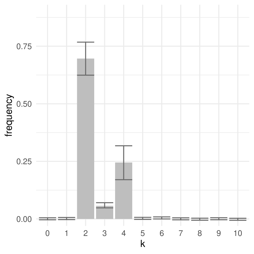
Figure 1: Estimated posterior distribution of $K$ with 95% simultaneous confidence intervals, $\varepsilon=1$ (left) and $\varepsilon=10^{-3}$ (right).

6.2 Variable selection in Bayesian probit regression

6.2.1 The model

Consider now the problem of variable selection in a Bayesian binary regression model.

Let $F(\cdot)$ be the cumulative distribution function of the standard normal distribution. For $i=1,\dots,N$, let $x_{i}=(x_{i,1},\dots,x_{i,r})^{\top}\in\mathbb{R}^{r}$ be a known vector of predictors. Let $Y_{1},\dots,Y_{N}$ be independent binary responses, where $Y_{i}$ follows a Bernoulli distribution with success probability $F(A+x_{i}^{\top}B)$. The scalar $A\in\mathbb{R}$ is an unknown intercept, while the vector $B=(B_{1},\dots,B_{r})^{\top}\in\mathbb{R}^{r}$ is an unknown regression coefficient.

To perform Bayesian variable selection, put a spike and slab prior on $B$. To be specific, let $K=(K_{1},\dots,K_{r})^{\top}$. Let $\mathcal{I}_{K}=\{j\in\{1,\dots,r\}:\,K_{j}=1\}$. Place a prior distribution on $K$ that has probability mass function proportional to $p^{|\mathcal{I}_{k}|}$, where $p\in(0,1)$ is a hyperparameter. Assume that given $K$, the $B_{i}$’s are independent. If $K_{i}=0$, $B_{i}$ is set to be zero; otherwise, $B_{i}$ follows the $\mbox{N}(0,\sigma^{2})$ distribution, where $\sigma$ is a positive hyperparameter. The intercept $A$ is independent of $(B,K)$ and follows the $\mbox{N}(0,\sigma^{2})$ distribution. Let $Z=(A,\eta_{K}(B)^{\top})^{\top}$, where $\eta_{K}$ extracts the elements of an $r$-dimensional vector whose indices are in $\mathcal{I}_{K}$. Then the model index $K$ indicates which predictors are relevant, and $Z$ is a vector of the intercept and the nonzero regression coefficients. Having observed $Y=(Y_{1},\dots,Y_{N})^{\top}$, the goal is to make inference about $(K,Z)$.

The parameter space, i.e., the range of $(K,Z)$, is $\mathsf{X}=\bigcup_{k\in\mathcal{K}}\{k\}\times\mathsf{Z}_{k}$, where $\mathcal{K}=\{0,1\}^{r}$ and $\mathsf{Z}_{k}=\mathbb{R}^{|\mathcal{I}_{k}|+1}$. The posterior distribution $\Pi$ of $(K,Z)$ given $Y=y=(y_{1},\dots,y_{n})$ is of the form (1). Evaluated at $z=(\alpha,\eta_{k}(\beta)^{\top})^{\top}$, where $\alpha\in\mathbb{R}$ and $\beta=(b_{1},\dots,b_{r})^{\top}\in\mathbb{R}^{r}$, the density function of $\Psi_{k}$ is

$$\pi(k,z\mid y)= \frac{1}{\sqrt{2\bm{\pi}}\sigma}\left(\frac{p}{\sqrt{2\bm{\pi}}\sigma}\right)^{|\mathcal{I}_{k}|}\exp\left(-\frac{\alpha^{2}+\sum_{j\in\mathcal{I}_{k}}b_{j}^{2}}{2\sigma^{2}}\right)$$

$$\prod_{i=1}^{N}F\left(\alpha+\eta_{k}(x_{i})^{\top}\eta_{k}(\beta)\right)^{y_{i}}\left[1-F\left(\alpha+\eta_{k}(x_{i})^{\top}\eta_{k}(\beta)\right)\right]^{1-y_{i}}.$$

6.2.2 A reversible jump MCMC algorithm

For a fixed model $k$, one can use a data augmentation algorithm (a type of reversible MCMC algorithm) devised by Albert and Chib (1993) to sample from $\Phi_{k}$, the normalization of $\Psi_{k}$. The algorithm is now briefly described. For $k\in\{0,1\}^{r}$, let $X(k)$ denote the $n\times(|\mathcal{I}_{k}|+1)$ matrix whose $i$th row is $x_{i}^{*}(k)^{\top}=(1,\eta_{k}(x_{i})^{\top})$. Given the current state $z\in\mathsf{Z}_{k}$, the next state $z^{\prime}$ is drawn through the following procedure: Independently, draw $u_{1},\dots,u_{N}$, where $u_{i}$ is a $\mbox{N}(x_{i}^{*}(k)^{\top}z,1^{2})$ random variable that is truncated to $(0,\infty)$ if $y_{i}=1$ and to $(-\infty,0)$ otherwise. Let $u=(u_{1},\dots,u_{N})^{\top}$. Draw $z^{\prime}$ from the normal distribution

$$\mbox{N}_{|\mathcal{I}_{k}|+1}\left(\left[X(k)^{\top}X(k)+\sigma^{-2}I_{|\mathcal{I}_{k}|+1}\right]^{-1}X(k)^{\top}u,\;\left[X(k)^{\top}X(k)+\sigma^{-2}I_{|\mathcal{I}_{k}|+1}\right]^{-1}\right).$$

The reversible jump MCMC algorithm considered herein is a combination of the data augmentation algorithm and a standard reversible jump scheme. Given the current state $(k,z)$, the algorithm randomly performs a U, B, or D move. It is assumed that the probability of choosing a move depends on $(k,z)$ only through $k$, and the probabilities are denoted by $q_{\scriptsize\mbox{U}}(k)$, $q_{\scriptsize\mbox{B}}(k)$, and $q_{\scriptsize\mbox{D}}(k)$, respectively.

• U move: Draw $z^{\prime}$ using one iteration of Albert and Chib’s data augmentation algorithm. Set the new state to $(k,z^{\prime})$.

• B move: Randomly and uniformly choose an index $j$ from $\mathcal{I}_{k}^{c}$, where the complement is taken with respect to the set $\{1,\dots,r\}$. Change the $j$th element of $k$ to one and call the resultant binary vector $k^{\prime}$. Draw $b$ from some distribution on $\mathbb{R}$ associated with a density function $g(\cdot\mid k,k^{\prime},z,y)$. Let $\alpha\in\mathbb{R}$ and $\beta\in\mathbb{R}^{r}$ be such that $(\alpha,\eta_{k}(\beta)^{\top})^{\top}=z$. Replace the $j$th element of $\beta$ by $b$, and call the resultant vector $\beta^{\prime}$. Let $z^{\prime}=(\alpha,\eta_{k^{\prime}}(\beta^{\prime})^{\top})^{\top}$. With probability

  $$\min\left\{1,\frac{\pi(k^{\prime},z^{\prime}\mid y)\,q_{\scriptsize\mbox{D}}(k^{\prime})\,(|\mathcal{I}_{k}|+1)^{-1}}{\pi(k,z\mid y)\,q_{\scriptsize\mbox{B}}(k)\,(r-|\mathcal{I}_{k}|)^{-1}g(b\mid k,k^{\prime},z,y)}\right\},$$

  set the next state to $(k^{\prime},z^{\prime})$; otherwise, keep the old state. This move type is available only when $|\mathcal{I}(k)|<r$.

• D move: Randomly and uniformly choose an index $j$ from $\mathcal{I}_{k}$. Change the $j$th element of $k$ to zero and call the resultant binary vector $k^{\prime}$. Let $\alpha\in\mathbb{R}$ and $\beta\in\mathbb{R}^{r}$ be such that $(\alpha,\eta_{k}(\beta)^{\top})^{\top}=z$, and set $z^{\prime}=(\alpha,\eta_{k^{\prime}}(\beta)^{\top})^{\top}$. Note that $z^{\prime}$ is just $z$ with an element deleted; call the deleted element $b$. With probability

  $$\min\left\{1,\frac{\pi(k^{\prime},z^{\prime}\mid y)\,q_{\scriptsize\mbox{B}}(k^{\prime})\,(r-|\mathcal{I}_{k}|+1)^{-1}g(b\mid k^{\prime},k,z^{\prime},y)}{\pi(k,z\mid y)\,q_{\scriptsize\mbox{D}}(k)\,|\mathcal{I}_{k}|^{-1}}\right\},$$

  set the next state to $(k^{\prime},z^{\prime})$; otherwise, keep the old state. This move type is available only when $|\mathcal{I}_{k}|>0$.

The resultant trans-dimensional chain is reversible with respect to $\Pi$.

6.2.3 Convergence analysis

Chakraborty and Khare (2017) proved the following result regarding the data augmentation algorithm of Albert and Chib (1993), which defines the U move type. The result is again established through drift and minorization. See also Roy and Hobert (2007).

Lemma 16.

For $k\in\mathcal{K}$, the data augmentation chain targeting $\Phi_{k}$ is $\Phi_{k}$-a.e. geometrically ergodic.

It is also well-known that, given $k$, the data augmentation chain of Albert and Chib (1993) is reversible with respect to $\Phi_{k}$. One can then establish geometric convergence for the reversible jump chain.

Proposition 17.

Suppose that $q_{\scriptsize\mbox{U}}(k)>0$ for $k\in\mathcal{K}$, $q_{\scriptsize\mbox{B}}(k)>0$ when $|\mathcal{I}_{k}|<r$, $q_{\scriptsize\mbox{D}}(k)>0$ when $|\mathcal{I}_{k}|>0$. Then the reversible jump chain is $L^{2}(\Pi)$-geometrically convergent and $\Pi$-a.e. geometrically ergodic.

Proof.

Apply Theorem 1. Let $P$ be the Mtk of the reversible jump chain. For $k\in\mathcal{K}=\{0,1\}^{r}$, let $P_{k}$ be the Mtk of the chain associated with the U move. By Lemma 16 and (i) of Lemma 3, $\|P_{k}\|_{\Phi_{k}}<1$ for $k\in\mathcal{K}$. It follows that, for $k\in\mathcal{K}$, (i) and (ii) of (H1) holds. Evidently, (iii) of (H1) also holds with $c_{k}=q_{\scriptsize\mbox{U}}(k)$.

To verify (H2), note that for $k,k^{\prime}\in\mathcal{K}$ and $z\in\mathsf{Z}_{k}$, $P^{s}((k,z),\{k^{\prime}\}\times\mathsf{Z}_{k^{\prime}})>0$ whenever $s$ is no less than the number of elements by which $k$ and $k^{\prime}$ differ. Thus, $P^{r}((k,z),\{k^{\prime}\}\times\mathsf{Z}_{k^{\prime}})>0$ for every pair of $k$ and $k^{\prime}$. By Lemma 2, (H2) holds with $s=r$.

The chain is thus $L^{2}(\Pi)$ geometrically convergent. It is also clearly $\varphi$-irreducible. By Lemma 4, it is $\Pi$-a.e. geometrically ergodic. ∎

6.2.4 Monte Carlo error assessment: Spam email detection

The reversible jump algorithm is applied to the Spambase data set (Hopkins et al., 1999). This data set contains $N=4601$ emails. The response $Y_{i}$ indicates whether the $i$th email is spam. Each email is associated with $r=57$ attributes, including the frequency of certain words and the length of sequences of consecutive capital letters. To perform variable selection, a spike and slab prior with $p=0.5$ is used.

In the B move of the reversible jump algorithm, $g(\cdot\mid k,k^{\prime},z,y)$ is chosen to be the density of a normal distribution. To specify the parameters of this normal distribution, some additional notations are needed. Recall that $k^{\prime}$ and $k$ differ by exactly one element, whose index is $j$, and $\alpha\in\mathbb{R}$ and $\beta\in\mathbb{R}^{r}$ satisfy $(\alpha,\eta_{k}(\beta)^{\top})^{\top}=z$. For $\tilde{b}\in\mathbb{R}$, let $z_{\tilde{b}}=(\alpha,\eta_{k^{\prime}}(\tilde{\beta})^{\top})^{\top}$, where $\tilde{\beta}$ is obtained by setting the $j$th element of $\beta$ to $\tilde{b}$. Then $\tilde{b}\mapsto\pi(k^{\prime},z_{\tilde{b}}\mid y)$ is a log-concave function. The mean of the normal distribution is the maximizer of this function, while the variance is the negative second-order derivative at the maximizer.

The probabilities of proposing birth and death moves are as follows:

$$q_{\scriptsize\mbox{B}}(k)=\frac{1}{3}\min\left\{1,\frac{p(r-|\mathcal{I}_{k}|)}{\mathcal{I}_{k}+1}\right\},\quad q_{\scriptsize\mbox{D}}(k)=\frac{1}{3}\min\left\{1,\frac{|\mathcal{I}_{k}|}{p(r-|\mathcal{I}_{k}|+1)}\right\}.$$

Under this construction, in the B move,

$$\frac{f_{K}(k^{\prime})q_{\scriptsize\mbox{D}}(k^{\prime})(|\mathcal{I}_{k}|+1)^{-1}}{f_{K}(k)q_{\scriptsize\mbox{B}}(k)(r-|\mathcal{I}_{k}|)^{-1}}=1.$$

By Proposition 17, the reversible jump chain is $\Pi$-a.e. geometrically ergodic.

A chain of length $n=10^{5}$ is simulated. The quantities of interest are the posterior probabilities of $K_{j}=1$ for $j=1,\dots,57$, i.e., the posterior probability of any given predictor being present in the regression model. 95% simultaneous confidence intervals are constructed for these quantities. The variance of the injected Gaussian noise is $0.1^{2}I_{57}$. The result is presented in Figure 2. This figure shows how important each predictor is according to the MCMC simulation, as well as the errors of their estimated importance.

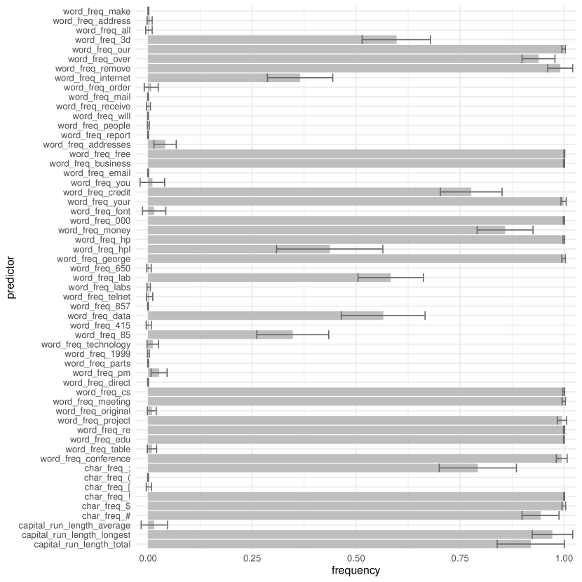
Figure 2: Estimated posterior probabilities of selecting each variable, with 95% simultaneous confidence intervals.

Acknowledgment: This work is partially supported by the National Science Foundation.

Appendices

Appendix A Proof of Lemma 2

It suffices to prove the following:

Lemma 18.

Let $s$ be a positive integer. Let $k,k^{\prime}\in\mathcal{K}$ be arbitrary, and assume that

$$\int_{\mathsf{Z}_{k}}\Psi_{k}(\mathrm{d}z)P^{s}((k,z),\{k^{\prime}\}\times\mathsf{Z}_{k^{\prime}})>0.$$ (13)

Then, one can find $s-1$ elements of $\mathcal{K}$, denoted by $k[1],\dots,k[s-1]$, such that $\prod_{t=0}^{s-1}\gamma_{k[t],k[t+1]}=1$, where $k[0]$ and $k[s]$ stand for $k$ and $k^{\prime}$, respectively. Consequently, if (13) holds for every pair of $k$ and $k^{\prime}$, then each element in $\Gamma_{P}^{s}$ is positive.

Proof.

The result holds when $s=1$. Assume that it holds for some $s=s^{\prime}\geq 1$. It suffices to prove it for $s=s^{\prime}+1$. To this end, let $k,k^{\prime}\in\mathcal{K}$ be arbitrary, and assume that

$$\int_{\mathsf{Z}_{k}}\Psi_{k}(\mathrm{d}z)P^{s^{\prime}+1}((k,z),\{k^{\prime}\}\times\mathsf{Z}_{k^{\prime}})>0.$$

Then there exists some $k^{\prime\prime}\in\mathcal{K}$ such that

$$\int_{\mathsf{Z}_{k}\times\mathsf{Z}_{k^{\prime\prime}}}\Psi_{k}(\mathrm{d}z)P^{s^{\prime}}((k,z),(k^{\prime\prime},\mathrm{d}z^{\prime\prime}))P((k^{\prime\prime},z^{\prime\prime}),\{k^{\prime}\}\times\mathsf{Z}_{k^{\prime}})>0.$$ (14)

This implies that

$$\int_{\mathsf{Z}_{k}}\Psi_{k}(\mathrm{d}z)P^{s^{\prime}}((k,z),\{k^{\prime\prime}\}\times\mathsf{Z}_{k^{\prime\prime}})>0.$$

Since the result holds for $s=s^{\prime}$, one can find $k[1],\dots,k[s^{\prime}-1]\in\mathcal{K}$ such that $\prod_{t=0}^{s^{\prime}-1}\gamma_{k[t],k[t+1]}=1$, where $k[0]=k$ and $k[s^{\prime}]=k^{\prime\prime}$. It remains to show that $\gamma_{k^{\prime\prime},k^{\prime}}=1$. Let $\mu$ be the measure on $(\mathsf{Z}_{k^{\prime\prime}},\mathcal{A}_{k^{\prime\prime}})$ such that

$$\mu(A)=\int_{\mathsf{Z}_{k}}\Psi_{k}(\mathrm{d}z)P^{s^{\prime}}((k,z),\{k^{\prime\prime}\}\times A),\quad A\in\mathcal{A}_{k^{\prime\prime}}.$$

Then (14) implies that the function $z^{\prime\prime}\mapsto P((k^{\prime\prime},z^{\prime\prime}),{k^{\prime}}\times\mathsf{Z}_{k^{\prime}})$ is not $\mu$-a.e. vanishing. On the other hand, $\mu$ is absolutely continuous with respect to $\Psi_{k^{\prime\prime}}$. This is because $\Pi=\Pi P^{s^{\prime}}$, which implies that

$$\Psi_{k^{\prime\prime}}(A)=\sum_{k^{\prime\prime\prime}\in\mathcal{K}}\Psi_{k^{\prime\prime\prime}}(\mathrm{d}z^{\prime\prime\prime})P^{s^{\prime}}((k^{\prime\prime\prime},z^{\prime\prime\prime}),\{k^{\prime\prime}\}\times A)\geq\mu(A),\quad A\in\mathcal{A}_{k^{\prime\prime}}.$$

Therefore, $z^{\prime\prime}\mapsto P((k^{\prime\prime},z^{\prime\prime}),{k^{\prime}}\times\mathsf{Z}_{k^{\prime}})$ is not $\Psi_{k^{\prime\prime}}$-a.e. vanishing. It follows that $\gamma_{k^{\prime\prime},k^{\prime}}=1$. ∎

Appendix B Proof of Lemma 6

Recall some notations: $(\mathsf{Y},\mathcal{F},\omega)$ is a probability space. $S$ and $T$ are Mtks that have $\omega$ as their stationary distributions. The state space $\mathsf{Y}$ has a disjoint decomposition $\mathsf{Y}=\bigcup_{k\in\mathcal{K}}\mathsf{Y}_{k}$. For $k\in\mathcal{K}$, $\mathcal{F}_{k}$ is the restriction of $\mathcal{F}$ to $\mathsf{Y}_{k}$, $\omega_{k}$ is the normalized restriction of $\omega$ on $\mathsf{Y}_{k}$, and $\bar{\omega}(\{k\})=\omega(\mathsf{Y}_{k})$. The Mtk $T_{k}:\mathsf{Y}_{k}\times\mathcal{F}_{k}\to[0,1]$ satisfies $\omega_{k}T_{k}=\omega_{k}$, and $T(y,B)\geq cT_{k}(y,B)$ for $y\in\mathsf{Y}_{k}$ and $B\in\mathcal{F}_{k}$, where $c\in[0,1]$. Finally, the kernel

$$\bar{S}(k,\{k^{\prime}\})=\frac{1}{\omega(\mathsf{Y}_{k})}\int_{\mathsf{Y}}\omega(\mathrm{d}y)S(y,\mathsf{Y}_{k})S(y,\mathsf{Y}_{k^{\prime}}).$$

defines a positive semi-definite operator on $L_{0}^{2}(\bar{\omega})$. The goal is to show that

$$1-\|TS^{*}\|_{\omega}^{2}\geq c^{2}\left(1-\sup_{k\in\mathcal{K}}\|T_{k}\|_{\omega_{k}}^{2}\right)(1-\|\bar{S}\|_{\bar{\omega}}).$$

Proof.

Let $f\in L_{0}^{2}(\omega)$ be arbitrary. Then

$$\|f\|_{\omega}^{2}-\|TS^{*}f\|_{\omega}^{2}=\|f\|_{\omega}^{2}-\|S^{*}f\|_{\omega}^{2}+\|S^{*}f\|_{\omega}^{2}-\|TS^{*}f\|_{\omega}^{2}.$$ (15)

For $y\in\mathsf{Y}$ and $B\in\mathcal{F}$, let

$$\hat{T}(y,B)=\sum_{k\in\mathcal{K}}1_{\mathsf{Y}_{k}}(y)T_{k}(y,B\cap\mathsf{Y}_{k}).$$

Then $\omega\hat{T}=\omega$, and $T(y,\cdot)\geq c\hat{T}(y,\cdot)$ for $y\in\mathsf{Y}$. Thus, there exists an Mtk $R:\mathsf{Y}\times\mathcal{F}\to[0,1]$ such that $\omega R=\omega$ and $T=c\hat{T}+(1-c)R$. Recall that the norms of Markov operators are no greater than one. Then

$$\|TS^{*}f\|_{\omega}^{2}= c^{2}\|\hat{T}S^{*}f\|_{\omega}^{2}+(1-c)^{2}\|RS^{*}f\|_{\omega}^{2}+2c(1-c)\langle\hat{T}S^{*}f,RS^{*}f\rangle_{\omega}$$

$$\leq c^{2}\|\hat{T}S^{*}f\|_{\omega}^{2}+(1-c^{2})\|S^{*}f\|^{2}.$$

It follows that

$$\|S^{*}f\|_{\omega}^{2}-\|TS^{*}f\|_{\omega}^{2}\geq c^{2}\left(\|S^{*}f\|_{\omega}^{2}-\|\hat{T}S^{*}f\|_{\omega}^{2}\right).$$ (16)

Define an operator $E:L_{0}^{2}(\omega)\to L_{0}^{2}(\omega)$ as

$$Ef(y)=\sum_{k\in\mathcal{K}}1_{\mathsf{Y}_{k}}(y)\frac{1}{\omega(\mathsf{Y}_{k})}\int_{\mathsf{Y}_{k}}\omega(\mathrm{d}y^{\prime})f(y^{\prime})=\sum_{k\in\mathcal{K}}1_{\mathsf{Y}_{k}}(y)\int_{\mathsf{Y}_{k}}\omega_{k}(\mathrm{d}y^{\prime})f(y^{\prime}).$$

Then $E$ is an orthogonal projection: $E^{2}=E^{*}=E$. Its range is the set of $L^{2}_{0}(\omega)$ functions that are constant on any given $\mathsf{Y}_{k}$. It is easy to see that $\hat{T}E=E$. In fact, $E\hat{T}=E$ as well. To see this, note that, for $g\in L_{0}^{2}(\omega)$,

$$E\hat{T}g(y) =\sum_{k\in\mathcal{K}}1_{\mathsf{Y}_{k}}(y)\int_{\mathsf{Y}_{k}}\omega_{k}(\mathrm{d}y^{\prime})\int_{\mathsf{Y}_{k}}T_{k}(y^{\prime},\mathrm{d}y^{\prime\prime})g(y^{\prime\prime})$$

$$=\sum_{k\in\mathcal{K}}1_{\mathsf{Y}_{k}}(y)\int_{\mathsf{Y}_{k}}\omega_{k}(\mathrm{d}y^{\prime\prime})g(y^{\prime\prime}).$$

It then follows that

$$\|S^{*}f\|_{\omega}^{2}-\|\hat{T}S^{*}f\|_{\omega}^{2}= \|[E+(I-E)]S^{*}f\|_{\omega}^{2}-\|\hat{T}[E+(I-E)]S^{*}f\|_{\omega}^{2}$$ (17)

$$= \|ES^{*}f\|_{\omega}^{2}+\|(I-E)S^{*}f\|_{\omega}^{2}-\|\hat{T}ES^{*}f\|_{\omega}^{2}-\|\hat{T}(I-E)S^{*}f\|_{\omega}^{2}-$$

$$2\langle\hat{T}ES^{*}f,\hat{T}(I-E)S^{*}f\rangle_{\omega}$$

$$= \|(I-E)S^{*}f\|_{\omega}^{2}-\|\hat{T}(I-E)S^{*}f\|_{\omega}^{2}.$$

($I$ is the identity operator.)

For $k\in\mathcal{K}$, let $M_{k}S^{*}f:\mathsf{Y}_{k}\to\mathbb{R}$ be such that

$$M_{k}S^{*}f(y)=(I-E)S^{*}f(y)=S^{*}f(y)-\int_{\mathsf{Y}_{k}}\omega_{k}(\mathrm{d}y^{\prime})S^{*}f(y^{\prime})$$

for $y\in\mathsf{Y}_{k}$. Then $M_{k}S^{*}f$ is in $L_{0}^{2}(\omega_{k})$, and

$$\|(I-E)S^{*}f\|_{\omega}^{2}=\sum_{k\in\mathcal{K}}\int_{\mathsf{Y}_{k}}\omega(\mathrm{d}y)\,[M_{k}S^{*}f(y)]^{2}=\sum_{k\in\mathcal{K}}\omega(\mathsf{Y}_{k})\|M_{k}S^{*}f\|_{\omega_{k}}^{2}.$$

Moreover,

$$\|\hat{T}(I-E)S^{*}f\|_{\omega}^{2} =\sum_{k\in\mathcal{K}}\int_{\mathsf{Y}_{k}}\omega(\mathrm{d}y)\,[T_{k}M_{k}S^{*}f(y)]^{2}$$ (18)

$$=\sum_{k\in\mathcal{K}}\omega(\mathsf{Y}_{k})\|T_{k}M_{k}S^{*}f\|_{\omega_{k}}^{2}$$

$$\leq\left(\sup_{k\in\mathcal{K}}\|T_{k}\|_{\omega_{k}}^{2}\right)\|(I-E)S^{*}f\|_{\omega}^{2}.$$

Combining (15) to (18) yields

$$\|f\|_{\omega}^{2}-\|TS^{*}f\|_{\omega}^{2} \geq\|f\|_{\omega}^{2}-\|S^{*}f\|_{\omega}^{2}+c^{2}\left(1-\sup_{k\in\mathcal{K}}\|T_{k}\|_{\omega_{k}}^{2}\right)\|(I-E)S^{*}f\|_{\omega}^{2}$$

$$\geq c^{2}\left(1-\sup_{k\in\mathcal{K}}\|T_{k}\|_{\omega_{k}}^{2}\right)\left[\|f\|_{\omega}^{2}-\|S^{*}f\|_{\omega}^{2}+\|(I-E)S^{*}f\|_{\omega}^{2}\right]$$

$$=c^{2}\left(1-\sup_{k\in\mathcal{K}}\|T_{k}\|_{\omega_{k}}^{2}\right)\left[\|f\|_{\omega}^{2}-\|ES^{*}f\|_{\omega}^{2}\right]$$

$$\geq c^{2}\left(1-\sup_{k\in\mathcal{K}}\|T_{k}\|_{\omega_{k}}^{2}\right)(1-\|ES^{*}\|_{\omega}^{2})\|f\|_{\omega}^{2}.$$

Since $f$ is arbitrary,

$$1-\|TS^{*}\|_{\omega}^{2}\geq c^{2}\left(1-\sup_{k\in\mathcal{K}}\|T_{k}\|_{\omega_{k}}^{2}\right)(1-\|ES^{*}\|_{\omega}^{2}).$$

To complete the proof, it suffices to show that $\|ES^{*}\|_{\omega}^{2}=\|\bar{S}\|_{\bar{\omega}}$. Note that $\|ES^{*}\|_{\omega}=\|(ES^{*})^{*}\|_{\omega}=\|SE\|_{\omega}$. Denote the range of $E$ by $H$. Then

$$\|ES^{*}\|_{\omega}^{2}=\|SE\|_{\omega}^{2}=\sup_{f\in L_{0}^{2}(\omega)\setminus\{0\}}\frac{\|SEf\|_{\omega}^{2}}{\|Ef\|_{\omega}^{2}+\|(I-E)f\|_{\omega}^{2}}=\sup_{f\in H\setminus\{0\}}\frac{\|Sf\|_{\omega}^{2}}{\|f\|_{\omega}^{2}}.$$ (19)

The transformation that maps a function $g:\mathcal{K}\to\mathbb{R}$ to $\sum_{k\in\mathcal{K}}g(k)1_{\mathsf{Y}_{k}}$ defines an isomorphism from $L_{0}^{2}(\bar{\omega})$ to $H$. Call this transformation $U$. Because $U$ is unitary,

$$\sup_{f\in H\setminus\{0\}}\frac{\|Sf\|_{\omega}^{2}}{\|f\|_{\omega}^{2}}=\sup_{g\in L_{0}^{2}(\bar{\omega})\setminus\{0\}}\frac{\|SUg\|_{\omega}^{2}}{\|g\|_{\bar{\omega}}^{2}}.$$ (20)

For $g\in L_{0}^{2}(\bar{\omega})$,

$$\|SUg\|_{\omega}^{2}=\int_{\mathsf{Y}}\omega(\mathrm{d}y)\left[\sum_{k\in\mathcal{K}}S(y,\mathsf{Y}_{k})g(k)\right]^{2}=\langle g,\bar{S}g\rangle_{\bar{\omega}}.$$ (21)

Note that $\bar{S}$ defines a positive semi-definite operator on $L_{0}^{2}(\bar{\omega})$. Then, by (19), (20), and (21), $\|ES^{*}\|_{\omega}^{2}=\|\bar{S}\|_{\bar{\omega}}$ as desired. ∎

Appendix C Proof of Lemma 9

Let $(\mathsf{Y},\mathcal{F},\omega)$ be a generic probability space and suppose that there is an Mtk $T$ such that $\omega=\omega T$. The lemma is restated below for the convenience of the reader.

Lemma 7. Suppose that there exists a function $R:\mathsf{Y}\times\{0,1,\dots\}\to[0,\infty)$ such that for $\omega$-a.e. every $y\in\mathsf{Y}$ and $t\geq 0$,

$$\|\delta_{y}T^{t}-\omega\|_{\scriptsize\mbox{TV}}\leq R(y,t).$$ (5)

Then there exists an Mtk $\hat{T}:\mathsf{Y}\times\mathcal{F}\to[0,1]$ such that (i) For $A,B\in\mathcal{F}$, $\int_{A}\omega(\mathrm{d}y)T(y,B)=\int_{A}\omega(\mathrm{d}y)\hat{T}(y,B)$, (ii) $\|\delta_{y}\hat{T}^{t}-\omega\|_{\scriptsize\mbox{TV}}\leq R(y,t)$ for every $y\in\mathsf{Y}$ and $t\geq 0$, and (iii) $T^{t}(y,\cdot)=\hat{T}^{t}(y,\cdot)$ for $y\in M^{c}$ and every $t\geq 0$, where $M\in\mathcal{F}$ is some set that satisfies $\omega(M)=0$. Moreover, for any distribution $\mu$ such that $\mu(M)=0$, on a suitably rich probability space one can construct two chains $Y(t)_{t=0}^{\infty}$ and $\hat{Y}(t)_{t=0}^{\infty}$ associated with $T$ and $\hat{T}$ respectively, such that $Y(0)\sim\mu$, and $Y(t)=\hat{Y}(t)$ for $t\geq 0$ with probability 1.

Proof.

By assumption, there exists $N_{0}\in\mathcal{F}$ such that $\omega(N_{0})=0$ and (5) holds for $y\in N_{0}^{c}$. Since $\omega$ is stationary for $T$, it must hold that $T(y,N_{0})=0$ for $\omega$-a.e. $y\in\mathsf{Y}$. In particular, there exists $N_{1}\supset N_{0}$ such that $\omega(N_{1})=0$, and $T(y,N_{0})=0$ for $y\in N_{1}^{c}$. By induction, there is an increasing sequence of sets $(N_{j})_{j=0}^{\infty}$ such that $\omega(N_{j+1})=0$ and $T(y,N_{j})=0$ whenever $y\in N_{j+1}^{c}$ for $j\geq 0$. Let $M=\bigcup_{j=0}^{\infty}N_{j}$. Then $\omega(M)=\lim_{j\to\infty}\omega(N_{j})=0$. For $y\in M^{c}=\bigcap_{j=0}^{\infty}N_{j+1}^{c}$, $T(y,N_{j})=0$ for each $j$, so $T(y,M)=\lim_{j\to\infty}T(y,N_{j})=0$.

Construct $\hat{T}$ as follows. For $y\in M^{c}$, let $\hat{T}(y,\cdot)=T(y,\cdot)$. For $y\in M$, let $\hat{T}(y,\cdot)=\omega(\cdot)$. (i) holds since, for $A,B\in\mathcal{F}$,

$$\int_{A}\omega(\mathrm{d}y)T(y,B)=\int_{A\cap M^{c}}\omega(\mathrm{d}y)T(y,B)=\int_{A\cap M^{c}}\omega(\mathrm{d}y)\hat{T}(y,B)=\int_{A}\omega(\mathrm{d}y)\hat{T}(y,B).$$

Assertion (iii) states that $T^{t}(y,\cdot)=\hat{T}^{t}(y,\cdot)$ for every $t$ whenever $y\in M^{c}$. This obviously holds when $t=1$. Suppose that this holds for a positive integer $t$. For $y\in M^{c}$, it was shown that $T(y,M)=\hat{T}(y,M)=0$. Thus, for $y\in M^{c}$ and $B\in\mathcal{F}$,

$$T^{t+1}(y,B)=\int_{M^{c}}T(y,\mathrm{d}y^{\prime})T^{t}(y^{\prime},B)=\int_{M^{c}}\hat{T}(y,\mathrm{d}y^{\prime})\hat{T}^{t}(y^{\prime},B)=\hat{T}^{t+1}(y,B).$$

By induction, (iii) holds. Note that, by (i), for $t\geq 1$, $\delta_{y}\hat{T}^{t}(\cdot)=\omega(\cdot)$ if $y\in M$, and by (iii), for $t\geq 0$, $\delta_{y}\hat{T}^{t}(\cdot)=\delta_{y}T^{t}(\cdot)$ if $y\in M^{c}$. Moreover, (5) holds for $y\in M^{c}$. Thus, (ii) holds.

It remains to construct $Y(t)$ and $\hat{Y}(t)$. Suppose that $\mu(M)=0$. Let $Y(0)\sim\mu$, and set $\hat{Y}(0)=Y(0)$. For $t\geq 0$, given $Y(t)$ and $\hat{Y}(t)$, draw $Y(t+1)$ and $\hat{Y}(t+1)$ using the following procedure: If $Y(t)\in M^{c}$ and $Y(t)=\hat{Y}(t)$, draw $Y(t+1)$ from the distribution $T(Y(t),\cdot)$, and let $\hat{Y}(t+1)=Y(t+1)$; otherwise, draw $Y(t+1)$ from $T(Y(t),\cdot)$, and independently draw $\hat{Y}(t+1)$ from $\hat{T}(\hat{Y}(t),\cdot)$. Evidently, $(Y(t),\hat{Y}(t))_{t=0}^{\infty}$ is a Markov chain whose transition kernel is

$$\tilde{T}((y,\hat{y}),(\mathrm{d}y^{\prime},\mathrm{d}\hat{y}^{\prime})) =\mathbf{1}_{\{y\}}(\hat{y})\mathbf{1}_{M^{c}}(y)T(y,\mathrm{d}y^{\prime})\delta_{y^{\prime}}(\mathrm{d}\hat{y}^{\prime})+[1-\mathbf{1}_{\{y\}}(\hat{y})\mathbf{1}_{M^{c}}(y)]T(y,\mathrm{d}y^{\prime})\hat{T}(\hat{y},\mathrm{d}\hat{y}^{\prime})$$

$$=\mathbf{1}_{\{\hat{y}\}}(y)\mathbf{1}_{M^{c}}(\hat{y})\hat{T}(\hat{y},\mathrm{d}\hat{y}^{\prime})\delta_{\hat{y}^{\prime}}(\mathrm{d}y^{\prime})+[1-\mathbf{1}_{\{\hat{y}\}}(y)\mathbf{1}_{M^{c}}(\hat{y})]T(y,\mathrm{d}y^{\prime})\hat{T}(\hat{y},\mathrm{d}\hat{y}^{\prime}).$$

Integrating out $\hat{y}^{\prime}$ shows that $(Y(t))_{t=0}^{\infty}$ is a Markov chain whose transition law is $T$, and integrating out $y^{\prime}$ shows that $(\hat{Y}(t))_{t=0}^{\infty}$ is a Markov chain whose transition law is $\hat{T}$. For $t\geq 0$,

$$\mbox{Pr}(Y(t^{\prime}+1)=\hat{Y}(t^{\prime}+1)\;\forall t^{\prime}\leq t) \geq\mbox{Pr}(Y(t^{\prime})\in M^{c}\;\forall t^{\prime}\leq t)$$

$$=\int_{M^{c}}\mu(\mathrm{d}y_{0})\int_{M^{c}}T(y_{0},\mathrm{d}y_{1})\cdots\int_{M^{c}}T(y_{t-1},\mathrm{d}y_{t})$$

$$=1.$$

Letting $t\to\infty$ shows that $(Y(t))_{t=0}^{\infty}=(\hat{Y}(t))_{t=0}^{\infty}$ with probability 1. ∎

Appendix D Proof of Lemma 14

Fix $k\in\mathcal{K}$. Suppose that $(A(t),B(t),T(t),U(t))_{t=0}^{\infty}$ is a chain associated with $P_{k}$. Then $(A(t),B(t),T(t))_{t=0}^{\infty}$ is also a Markov chain that has the same convergence rate in the total variation distance. This is because the two chains are co-de-initializing (Roberts and Rosenthal, 2001). Thus, it suffices to show that the latter is $\hat{\Phi}_{k}$-a.e. geometrically ergodic, where $\hat{\Phi}_{k}$ is the distribution of $(A,B,T)$ given $(K,Y)=(k,y)$.

To show geometric ergodicity one can establish a set of drift and minorization conditions (Rosenthal, 1995). Let $\hat{P}_{k}$ be the Mtk of $(A(t),B(t),T(t))_{t=0}^{\infty}$. For $(\alpha,\beta,\tau)\in\mathbb{R}^{k}\times\mathbb{R}^{p}\times(0,\infty)$, let

$$V(\alpha,\beta,\tau)=\frac{\sum_{i=1}^{N}(y_{i}-x_{i}^{\top}\beta-w_{i,k}^{\top}\alpha)^{2}}{\tau}.$$

The following two lemmas establish a set of drift and minorization conditions for $\hat{P}_{k}$. Similar arguments can be found in, e.g., Roy and Hobert (2010) and Hobert et al. (2018).

Lemma 19.

Assume that (P1) holds. There exist $\lambda<1$ and $L<\infty$ such that the following holds for each $(\alpha,\beta,\tau)\in\mathbb{R}^{k}\times\mathbb{R}^{p}\times(0,\infty)$:

$$\hat{P}_{k}V(\alpha,\beta,\tau)\leq\lambda V(\alpha,\beta,\tau)+L.$$

Proof.

Fix $(\alpha,\beta,\tau)\in\mathbb{R}^{k}\times\mathbb{R}^{p}\times(0,\infty)$. Let $(A^{\prime},B^{\prime},T^{\prime})\sim\hat{P}_{k}((\alpha,\beta,\tau),\cdot)$. Recalling the steps of the two-component Gibbs algorithm, one can obtain

$$\hat{P}_{k}V(\alpha,\beta,\tau)= E\left[V(A^{\prime},B^{\prime},T^{\prime})\right]$$

$$= E\left\{\frac{\|y-W(k)[W(k)^{\top}QW(k)+\sigma^{-2}I_{p+k}]^{-1}W(k)^{\top}Qy\|^{2}}{T^{\prime}}\right\}+$$

$$E\left(\mbox{tr}\left\{W(k)[W(k)^{\top}QW(k)+\sigma^{-2}I_{p+k}]^{-1}W(k)^{\top}\right\}\right)$$

$$= E\left\{\frac{N\|y-W(k)[W(k)^{\top}QW(k)+\sigma^{-2}I_{p+k}]^{-1}W(k)^{\top}Qy\|^{2}}{y^{\top}Qy-y^{\top}QW(k)[W(k)^{\top}QW(k)+\sigma^{-2}I_{p+k}]^{-1}W(k)^{\top}Qy}\right\}+$$

$$E\left(\mbox{tr}\left\{W(k)[W(k)^{\top}QW(k)+\sigma^{-2}I_{p+k}]^{-1}W(k)^{\top}\right\}\right),$$

where $W(k)$ is the $N\times(p+k)$ matrix whose $i$th row is $(x_{i}^{\top},w_{i,k}^{\top})$, and $Q$ is the $N\times N$ diagonal matrix whose diagonal elements $(U_{1}^{\prime},\dots,U_{N}^{\prime})$ are distributed according to the density

$$f_{U\mid\cdot}(u^{\prime}\mid k,\alpha,\beta,\tau,y)$$

$$= \prod_{i=1}^{N}\left\{\frac{1}{\sqrt{8\bm{\pi}u_{i}^{\prime 3}}}\exp\left[-\frac{u_{i}^{\prime}(y_{i}-x_{i}^{\top}\beta-w_{i,k}^{\top}\alpha)^{2}}{2\tau}+\frac{|y_{i}-x_{i}^{\top}\beta-w_{i,k}^{\top}\alpha|}{2\sqrt{\tau}}-\frac{1}{8u_{i}^{\prime}}\right]\,\mathbf{1}_{(0,\infty)}(u_{i}^{\prime})\right\}.$$

Under (P1), $Q^{1/2}y$ is not in the column space of $Q^{1/2}W(k)$. This implies that

$$y^{\top}Qy-y^{\top}QW(k)[W(k)^{\top}QW(k)+\sigma^{-2}I_{p+k}]^{-1}W(k)^{\top}Qy$$

$$\geq y^{\top}Qy-y^{\top}QW(k)[W(k)^{\top}QW(k)]^{-1}W(k)^{\top}Qy$$

$$= \left\|\left\{I_{N}-Q^{1/2}W(k)[W(k)^{\top}QW(k)]^{-1}W(k)^{\top}Q^{1/2}\right\}Q^{1/2}y\right\|^{2}$$

$$> 0.$$

Moreover,

$$y^{\top}Qy-y^{\top}QW(k)[W(k)^{\top}QW(k)+\sigma^{-2}I_{p+k}]^{-1}W(k)^{\top}Qy$$

$$\geq \left\|Q^{1/2}\left\{y-W(k)[W(k)^{\top}QW(k)+\sigma^{-2}I_{p+k}]^{-1}W(k)^{\top}Qy\right\}\right\|^{2}$$

$$\geq \left(\min_{i}U_{i}^{\prime}\right)\|y-W(k)[W(k)^{\top}QW(k)+\sigma^{-2}I_{p+k}]^{-1}W(k)^{\top}Qy\|^{2},$$

and

$$\mbox{tr}\left\{W(k)[W(k)^{\top}QW(k)+\sigma^{-2}I_{p+k}]^{-1}W(k)^{\top}\right\}$$

$$\leq \mbox{tr}\left\{W(k)[W(k)^{\top}QW(k)]^{-1}W(k)^{\top}\right\}$$

$$\leq \left(\max_{i}U_{i}^{-1}\right)\mbox{tr}\left\{W(k)[W(k)^{\top}W(k)]^{-1}W(k)^{\top}\right\}$$

$$= (p+k)\left(\max_{i}U_{i}^{\prime-1}\right).$$

It follows that

$$\hat{P}_{k}V(\alpha,\beta,\tau)\leq(N+p+k)E\left(\max_{i}U_{i}^{\prime-1}\right)\leq(N+p+k)\sum_{i=1}^{N}E(U_{i}^{\prime-1}).$$

Using properties of the inverse Gaussian distribution and the Cauchy-Schwarz inequality, one obtains

$$\hat{P}_{k}V(\alpha,\beta,\tau) \leq(N+p+k)\sum_{i=1}^{N}\left(\frac{2|y_{i}-x_{i}^{\top}\beta-w_{i,k}^{\top}\alpha|}{\sqrt{\tau}}+4\right)$$

$$\leq 2(N+p+k)\sqrt{N}\sqrt{V(\alpha,\beta,\tau)}+4(N+p+k).$$

The desired result follows immediately. ∎

Lemma 20.

For each $d>0$, there exists a nonzero measure $\nu(\cdot)$

$$\hat{P}_{k}((\alpha,\beta,\tau),\cdot)\geq\nu(\cdot)$$

whenever $V(\alpha,\beta,\tau)\leq d$.

Proof.

Denote the conditional density of $(A,B,T)$ given $(K,U,Y)=(k,u,y)$ by $f_{A,B,T\mid\cdot}(\cdot\mid k,u,y)$. Then the density of $\hat{P}_{k}((\alpha,\beta,\tau),\cdot)$ is

$$\int_{(0,\infty)^{N}}f_{A,B,T\mid\cdot}(\cdot\mid k,y)\,f_{U\mid\cdot}(u\mid k,\alpha,\beta,\tau,u,y)\,\mathrm{d}u.$$

Assume that $V(\alpha,\beta,\tau)\leq d$, so that $(y_{i}-x_{i}^{\top}\beta-w_{i,k}^{\top}\alpha)^{2}/\tau\leq d$ for $i=1,\dots,N$. Then, for $u=(u_{1},\dots,u_{n})\in(0,\infty)^{N}$,

$$f_{U\mid\cdot}(u\mid k,\alpha,\beta,\tau,y)\geq\prod_{i=1}^{N}\left[\frac{1}{\sqrt{8\bm{\pi}u_{i}^{3}}}\exp\left(-\frac{du_{i}}{2}-\frac{1}{8u_{i}}\right)\right].$$

The desired result is established by letting $\nu$ be associated with the density

$$\int_{(0,\infty)^{N}}f_{A,B,T\mid\cdot}(\cdot\mid k,u,y)\prod_{i=1}^{N}\left[\frac{1}{\sqrt{8\bm{\pi}u_{i}^{3}}}\exp\left(-\frac{du_{i}}{2}-\frac{1}{8u_{i}}\right)\right]\,\mathrm{d}u.$$

∎

By Lemmas 19 and 20 and the standard drift and minorization argument (Rosenthal, 1995), $\hat{P}_{k}$ is $\hat{\Phi}_{k}$-a.e. geometrically ergodic. As previously mentioned, this implies that $P_{k}$ is $\Phi_{k}$-a.e. geometrically ergodic.

References

- Albert and Chib (1993) Albert, J. H. and Chib, S. (1993). Bayesian analysis of binary and polychotomous response data. Journal of the American Statistical Association 88 669–679.
- Andrieu and Doucet (1999) Andrieu, C. and Doucet, A. (1999). Joint Bayesian model selection and estimation of noisy sinusoids via reversible jump MCMC. IEEE Transactions on Signal Processing 47 2667–2676.
- Banerjee and Vats (2022) Banerjee, A. and Vats, D. (2022). Multivariate strong invariance principles in Markov chain Monte Carlo. arXiv preprint arXiv:2211.06855 .
- Caracciolo et al. (1992) Caracciolo, S., Pelissetto, A. and Sokal, A. D. (1992). Two remarks on simulated tempering. Unpublished manuscript.