Study of multinucleon transfer mechanism in ${}^{160}\text{Gd}+{}^{186}\text{W}$ collisions in stochastic mean-field theory

Abstract

Multinucleon transfer mechanism in collision of ${}^{160}\text{Gd}+{}^{186}\text{W}$ system is investigated in the framework of quantal transport description, based on the stochastic mean-field (SMF) theory. The SMF theory provides a microscopic approach for nuclear dynamics beyond the time-dependent Hartree-Fock (TDHF) approach by including mean-field fluctuations. Cross-sections for the primary fragment production are determined in the quantal transport description and compared with the available data.

I Introduction

Production of heavy elements near the superheavy island with proton numbers $Z>100$ embodies one of the greatest experimental and theoretical challenges [1, 2, 3, 4, 5, 6, 7, 8, 9, 10, 11, 12, 13, 14, 15, 16]. The most common approach for the production of these elements and their isotopes is through fusion reactions. Historically, two distinct experimental approaches have been employed to synthesize these nuclei, named based on their excitation properties, as cold fusion reactions [17] and hot fusion reactions [18, 14]. The primary composite systems formed in these reactions are at a relatively high excitation energy, which subsequently de-excites by emitting neutrons, alpha particles, and secondary fission. This results in an exceedingly small evaporation residue cross-sections that makes reaching to heavier elements as well as the neutron rich isotopes of these elements very difficult. To circumvent this obstacle multi-nucleon transfer reactions have been proposed as an alternative. Such experiments recently focused on using actinide targets at near the Coulomb barrier energies. Using this approach it is possible to produce heavy primary fragments at reasonably lower excitation energies. Consequently, such reactions may provide a more efficient mechanism for production of heavy neutron-rich isotopes, than fusion, fission, and fragmentation reactions. In collision involving deformed target nuclei multinucleon transfer depends on the collision geometry. In a typical collision, the system drifts toward symmetry. However, for certain geometries the system may drift toward asymmetry, which is referred to as inverse quasi-fission. Multinucleon transfer mechanism has been studied by employing a number of phenomenological approaches, such as the multidimensional Langevin model [19, 20, 21, 22, 23, 24, 25], di-nuclear system model [26, 27, 28], and the quantum molecular dynamics approach [29, 30, 31].

To formulate a reliable description of the multiparticle transfer mechanism and its dependence on the collision geometry it is essential to utilize microscopic approaches. Time-Dependent Hartree-Fock (TDHF) theory is a good candidate as the basis for such a microscopic description to describe the evolution of collective dynamics at low bombarding energies [32, 33, 34, 35, 36, 37, 38, 39, 40, 41]. Despite its success, TDHF theory, based on the mean-field approach, only describes the most probable path of the collision dynamics with small fluctuations around it. By virtue of this limitation TDHF generally describes the mean values of observables, such as the kinetic energy loss involving one-body dissipation, but is unable to account for larger fluctuations and dispersions of the fragment mass and charge distributions. In order to account for these observables it is necessary to find a prescription that goes beyond the mean-field approximation [42, 43, 44, 45, 46]. One such approach is through the time-dependent random phase approximation (TDRPA) developed by Balian and Vénéroni, which provides a consistent theory to computer larger fluctuations of the observables going beyond mean-field. This method has been used to study multinucleon transfer reactions in symmetric systems [47, 48, 49, 50, 51], it is inherently constrained to compute the dispersion of charge and mass distributions in symmetric collisions.

The stochastic mean-field (SMF) theory, closely related to TDRPA, circumvents this problem and facilitates further improvements to the beyond mean field approximation [45, 46]. The manuscript is organized as follows: In Sec. II, we provide results of TDHF calculations for the collisions of the ${}^{160}\text{Gd}+{}^{186}\text{W}$ system at E${}_{\text{c.m.}}=$502.6 MeV and E${}_{\text{c.m.}}=$461.9 MeV. Section III briefly describes multi-nucleon transfer as constituted in the quantal transport description of the SMF approach. In this reaction both projectile and target nuclei are two deformed isotopes between doubly closed ¹³²Sn and ²⁰⁸Pb shells (Z=50, N=82 and Z=82, N=126). For most collision geometries, initial mass asymmetry increases, which cause reaction to be characterized as inverse quasi-fission. In Sec. IV, we provide the analysis of multinucleon transfer mechanism for the same reaction. The quantal transport approach describes the production of primary isotopes and we compare results with the available data [52]. The cross-section distributions, mean values, and dispersions are determined without any adjustable parameter employing a Skyrme energy density functional. In Sec. V, we summarize our results and provide conclusions.

II Mean-Field Properties

The TDHF theory has been the primary microscopic tool for studying low-energy heavy-ion reactions, including fusion, deep-inelastic collisions, and quasifission[32, 34, 35, 36, 39, 40, 33, 41]. Since the theory is derived by the minimization of the time-dependent many-body action it is deterministic in nature and provides the most probably reaction path for the system. Namely, given a set of initial conditions for the reaction there is only one outcome for the reaction. At some level distribution can be obtained by varying the initial conditions (e.g. orbital angular momentum or the orientation angle for deformed nuclei). However, these distributions are typically much narrower when compared with the experiment. TDHF also provides a good description of one-body dissipation [53, 54]. In system ${}^{160}\text{Gd}+{}^{186}\text{W}$, initial ground states for the target and the projectile have large prolate deformations. Consequently, the reaction dynamics and the transfer of nucleons depend on the relative alignment of the target and projectile. We refer to this as the dependence on collision geometry. For the reaction ${}^{160}\text{Gd}+{}^{186}\text{W}$, at initial energies E${}_{\text{c.m.}}$ = 461.9 MeV and E${}_{\text{c.m.}}$ = 502.6 MeV, we explore four distinct alignments of the target and the projectile. Using the convention adopted in the work of Kedziora and Simenel, in Ref. [55], we denote initial orientation of either the projectile or the target principle deformation axis to be in the beam direction with X, and the case when their principle axis is perpendicular to the beam direction with Y. As a result we are faced with four distinct orientation possibilities for the target and the projectile, labeled as YY, XX, XY, YX corresponding to side-side, tip-tip, tip-side, and side-tip collision geometries, respectively (please see Fig. 2 and Fig. 3 in Ref. [55]. Here, the first letter stands for the orientation of the lighter collision partner. The calculations presented in the rest of the article employed the TDHF code [56, 57] using the SLy4d Skyrme energy density functional [58], with a box size of $60\times 60\times 36$ fm in the $x-y-z$ directions, respectively. The results of our TDHF calculations for all of these collision geometries are tabulated in Tables 1 and 2 at two bombarding energies and for a range of initial orbital angular momenta $\ell_{i}$. We denote the final values of mass and charge numbers for the Gd-like fragments with $A_{1}^{f}$, $Z_{1}^{f}$, and W-like fragment with $A_{2}^{f}$, $Z_{2}^{f}$, final total kinetic energy lost (TKEL), scattering angles in the c.m. $\theta_{\text{c.m.}}$, and laboratory frame, $\theta_{1}^{lab}$ and $\theta_{2}^{lab}$. These tables also include asymptotic values of neutron $\sigma_{NN}$, proton $\sigma_{ZZ}$, mixed dispersions $\sigma_{NZ}$ and mass dispersions $\sigma_{AA}$, which will be discussed in Sec. III. To economize on the computation time all quantities are evaluated in steps of 20 units of orbital angular momentum. The range of initial orbital angular momenta is specified according to the angular position of detectors in the laboratory system. The values of initial orbital angular momenta, which fall into detector acceptance range of $25^{\circ}-65^{\circ}$ in the laboratory frame, are shown in Table 1 and Table 2. At the lower collision energy, E${}_{\text{c.m.}}$ = 461.9 MeV, only in the tip-tip and tip-side geometries produced fragments fall in the acceptance range of detectors. As a result, in Table 2 only the tip-tip and tip-side results are shown. Different collision geometries have qualitatively distinct nucleon transfer mechanisms. These can be seen more clearly by plotting the time evolution of neutron $N(t)$ and proton $Z(t)$ numbers for Gd-like fragments or W-like fragments. In Fig. 1A of Appendix A, time evolution of proton and neutron numbers of W-like fragments in central collision of ${}^{160}\text{Gd}+{}^{186}\text{W}$ are presented at different collision geometries.

Table 1: Results of the TDHF and SMF calculations for the ${}^{160}\text{Gd}+{}^{186}\text{W}$ system at $E_{\text{c.m.}}=502.6$ MeV in tip-tip (XX), tip-side (XY), side-tip (YX) and side-side (YY) geometries.

Geometry	$\ell_{i}$ $(\hbar)$	$Z_{1}^{f}$	$A_{1}^{f}$	$Z_{2}^{f}$	$A_{2}^{f}$	$\ell_{f}$ $(\hbar)$	$TKEL$	$\sigma_{NN}$	$\sigma_{ZZ}$	$\sigma_{NZ}$	$\sigma_{AA}$	$\theta_{\text{c.m.}}$	$\theta_{1}^{lab}$	$\theta_{2}^{lab}$
XX	120	61.1	152.7	76.9	193.3	117.1	245.7	5.8	4.3	3.9	9.1	120.8	55.0	24.1
	140	64.2	160.5	73.8	185.5	125.2	237.0	5.7	4.3	3.9	9.0	114.3	51.1	27.6
	160	65.8	164.5	72.2	181.5	134.0	208.2	5.6	4.2	3.7	8.8	111.8	51.1	30.0
	180	65.5	164.0	72.5	182.0	120.8	173.5	5.4	4.1	3.5	8.4	111.7	53.4	31.0
	200	65.6	164.3	72.4	181.7	138.0	140.5	5.1	3.9	3.2	7.9	107.5	53.2	33.9
	220	65.2	163.5	72.8	182.5	165.9	114.7	4.8	3.5	2.7	7.1	102.8	52.2	36.6
	240	64.5	161.8	73.5	184.2	202.3	85.3	4.1	2.9	1.9	5.7	98.7	51.7	39.1
XY	120	61.2	152.6	76.8	193.4	116.9	212.3	7.1	4.9	5.2	11.3	120.8	57.9	24.9
	140	64.7	161.6	73.3	184.4	132.8	212.6	6.9	4.8	5.0	11.0	113.6	52.3	28.8
	160	65.4	163.3	72.6	182.7	136.9	186.0	6.6	4.5	4.7	10.4	110.6	52.3	31.1
	180	65.3	163.3	72.7	182.7	141.2	169.3	6.2	4.3	4.3	9.7	106.8	51.6	33.2
	200	65.3	163.3	72.7	182.7	154.1	155.3	5.9	4.1	4.0	9.1	102.6	50.3	35.5
	220	65.1	163.0	72.9	183.0	170.6	136.3	5.4	3.8	3.5	8.3	99.0	49.5	37.6
	240	64.9	162.3	73.1	183.7	191.2	113.8	4.8	3.4	2.9	7.1	96.1	49.0	39.6
	260	64.4	161.5	73.6	184.5	218.8	81.9	3.9	2.7	1.9	5.4	94.1	49.3	41.4
YX	120	66.3	166.3	71.7	179.6	98.1	177.3	6.5	4.6	4.6	10.3	123.2	57.5	26.0
	140	66.1	165.5	71.9	180.5	117.4	162.3	6.2	4.3	4.2	9.6	117.2	56.2	29.0
	160	65.8	164.7	72.2	181.3	130.8	146.4	5.8	4.1	3.9	9.0	112.6	55.3	31.4
	180	65.9	165.0	72.1	181.0	148.2	134.2	5.5	3.8	3.5	8.4	107.9	53.5	33.9
	200	65.3	163.8	72.7	182.2	168.5	122.0	5.0	3.5	3.0	7.4	103.6	52.2	36.1
	220	64.5	162.1	73.5	183.9	186.0	101.8	4.4	3.0	2.3	6.3	100.4	51.8	37.9
	240	64.1	161.0	73.9	185.0	217.5	73.5	3.7	2.5	1.6	4.9	97.9	51.8	39.7
YY	120	64.1	159.8	73.9	186.2	106.7	123.1	5.4	3.7	3.5	8.3	125.7	64.7	25.4
	140	64.4	160.8	73.6	185.2	123.4	113.8	5.1	3.5	3.3	7.7	120.1	62.0	28.3
	160	64.6	161.5	73.4	184.5	141.2	105.6	4.8	3.3	2.9	7.2	115.0	59.6	30.9
	180	64.6	161.6	73.4	184.4	159.4	95.6	4.5	3.1	2.6	6.5	110.6	57.7	33.2
	200	64.4	161.4	73.6	184.6	175.4	81.4	4.0	2.8	2.1	5.7	106.9	56.3	35.3
	220	64.3	161.2	73.7	184.8	193.2	66.3	3.6	2.4	1.6	4.8	103.7	55.3	37.1

Table 2: Results of the TDHF and SMF calculations for the ${}^{160}\text{Gd}+{}^{186}\text{W}$ system at $E_{\text{c.m.}}=461.9$ MeV in tip-tip (XX), tip-side (XY) geometries.

Geometry	$\ell_{i}$ $(\hbar)$	$Z_{1}^{f}$	$A_{1}^{f}$	$Z_{2}^{f}$	$A_{2}^{f}$	$\ell_{f}$ $(\hbar)$	$TKEL$	$\sigma_{NN}$	$\sigma_{ZZ}$	$\sigma_{NZ}$	$\sigma_{AA}$	$\theta_{\text{c.m.}}$	$\theta_{1}^{lab}$	$\theta_{2}^{lab}$
XX	140	65.0	162.6	73.0	183.4	88.9	97.7	5.1	3.8	3.1	7.7	129.7	65.8	23.8
	160	64.9	162.7	73.1	183.3	116.1	81.4	4.7	3.5	2.7	7.0	123.3	63.7	27.1
	180	64.4	161.5	73.6	184.5	149.7	56.7	4.1	3.0	2.0	5.8	117.9	62.6	30.1
XY	140	64.6	161.8	73.4	184.2	117.2	75.2	4.8	3.3	2.8	7.1	126.3	66.0	25.7
	160	64.5	161.7	73.5	184.3	138.2	59.2	4.3	3.0	2.3	6.1	121.3	64.3	28.4

We can extract more useful information about nucleon transfer mechanisms by examining drift paths. Drift paths are obtained by eliminating time from neutron $N(t)$ and proton numbers $Z(t)$ and plotting the result in $(N,Z)$ plane. Drift paths in different collision geometries exhibit a different behavior as a results of the shell effects on the dynamics, and contain specific information about the time evolution of the mean values of macroscopic variables. In Fig. 1 we plot drift paths for head-on collisions in different geometries for W-like fragments (blue curves). In these figures, thick black lines denote set of fragments with charge asymmetry value of $\frac{N-Z}{N+Z}=0.20$. These lines are called the iso-scalar path, which travel near the bottom of stability valley. The iso-scalar path extends all the way from lead valley on the upper end and toward the barium valley on the lower end, and it makes about $\phi=33^{\circ}$ with the horizontal neutron axis. We observe that in all geometries, W-like fragments drift along iso-scalar direction with a charge asymmetry of approximately 0.20. Fig. 1(a) shows the drift path in tip-tip (XX) collisions. Initially, as seen usually in quasi-fission reactions, W-like heavy fragments loses nucleons and the system drifts toward symmetry. After this initial behavior, W-like heavy fragments turn back and by gaining nucleons drift toward asymmetry. This kind of drift path is not very usual and it is referred to as inverse quasi-fission reaction. Fig. 1(b) shows drift path in tip-side (XY) collision. In this case, drift path also indicates an inverse quasi-fission reaction. In side-tip (YX) collision, shown in Fig. 1(c), nucleon drift mechanism is similar to the tip-tip (XX) geometry. Initially, heavy fragment loses neuron and protons and system drifts along iso-scalar path toward symmetry, subsequently changing direction and drifting toward asymmetry. As seen in Fig. 1(d), in side-side (YY) collision drift mechanism is analogous to the one for side-tip collision.

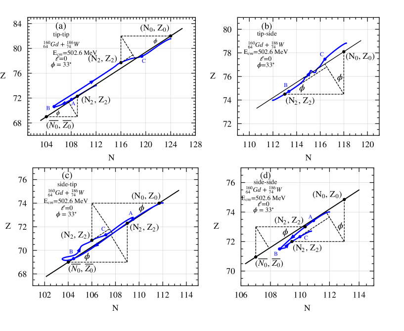
Figure 1: Blue curves show drift path of W-like fragments in the head-on collision of ${}^{160}\text{Gd}+{}^{186}\text{W}$ system at $E_{\text{c.m.}}=502.6$ MeV in tip-tip (a), tip-side (b), side-tip (c) and side-side (d) geometries.

III Quantal Diffusion of Nucleon Transfer

III.1 Langevin equations for multinucleon transfer

In TDHF theory, with a prescribed set of initial conditions, the many-body state is a single Slater determinant and a unique single-particle density matrix, that is time-dependent describing the deterministic reaction path for the dynamical system. In beyond TDHF approaches, introducing additional correlations are typically represented by a superposition of Slater determinants. In the SMF theory, correlations are introduced as fluctuations of the initial state, which constitute an ensemble of single-particle density matrices [45, 46]. For each of these single-particle density matrices in the ensemble, the time-evolution reduces to the TDHF equations initialized by the self-consistent Hamiltonian of the particular event. In constructing the fluctuations of these initial density matrices SMF employs a Gaussian distribution of the random elements with variances that are specified with the requirement that ensemble average of the one-body operator dispersions of the initial state are the same as the ones obtained in the quantal expressions in the mean-field approach.

For low-energy heavy-ion collisions at energies near the Coulomb barrier the dynamical system generally maintains a di-nuclear configuration. In these cases instead of generating an ensemble of mean-field events one can formulate a more straight forward transport approach. Using the window dynamics of the di-nuclear system one can do a geometric projection of the SMF approach to obtain Langevin equations for the relevant macroscopic variables. For the derivations of the quantal diffusion formalism and the utilization of window dynamics we refer the reader to earlier references [59, 60, 61, 62, 63, 64, 65]. Neutron and proton number of the projectile-like or target-like fragment are chosen as the relevant macroscopic variables to formulate the diffusion formalism. For the system at hand, we take neutron $N_{2}^{\lambda}(t)$ and proton $Z_{2}^{\lambda}(t)$ numbers of the W-like fragments as relevant macroscopic variables. For each event, $\lambda$, the fragment neutron and proton numbers are obtained by integrating the density on the left and right of the window. During the contact phase, fragment proton and neutron numbers fluctuate between events as a result of random nucleon flux through the window. These numbers can be decomposed as fluctuations about the mean values as $N_{2}^{\lambda}(t)=N_{2}(t)+\mathit{\delta N}_{1}^{\lambda}(t)$ and $Z_{2}^{\lambda}(t)=Z_{2}(t)+\mathit{\delta Z}_{2}^{\lambda}(t)$. Here, $N_{2}(t)$ and $Z_{2}(t)$ are the mean values obtained over the ensemble of SMF events.

These mean values can be deduced from the mean-field TDHF calculations for small amplitude fluctuations. In the quantal diffusion approach, for small amplitude fluctuations, neutron $\mathit{\delta N}_{2}^{\lambda}(t)$ and proton $\mathit{\delta Z}_{2}^{\lambda}(t)$ numbers evolve according to a coupled linear set of quantal Langevin equations,

$$\frac{d}{dt}\left(\begin{array}[]{c}{\delta Z_{2}^{\lambda}(t)}\\ {\delta N_{2}^{\lambda}(t)}\end{array}\right)= \left(\begin{array}[]{c}{\frac{\partial v_{p}}{\partial Z_{2}}\left(Z_{2}^{\lambda}-Z_{2}\right)+\frac{\partial v_{p}}{\partial N_{2}}\left(N_{2}^{\lambda}-N_{2}\right)}\\ {\frac{\partial v_{n}}{\partial Z_{2}}\left(Z_{2}^{\lambda}-Z_{2}\right)+\frac{\partial v_{n}}{\partial N_{2}}\left(N_{2}^{\lambda}-N_{2}\right)}\end{array}\right)$$ (5)

$$+\left(\begin{array}[]{c}{\delta v_{p}^{\lambda}(t)}\\ {\delta v_{n}^{\lambda}(t)}\end{array}\right).$$ (8)

Quantities $v_{\alpha}^{\lambda}(t)=v_{\alpha}(t)+\delta v_{\alpha}^{\lambda}(t)$ denote the drift coefficients for protons and neutrons, with the mean values and the fluctuating parts given by $v_{\alpha}(t)$ and $\mathit{\delta v}_{\alpha}^{\lambda}(t)$, respectively. Here, the index $\alpha$ labels protons and neutrons. Drift coefficients $v_{\alpha}^{\lambda}(t)$, denote the rate of flux for protons and neutrons through the window in event $\lambda$. The linear limit of Langevin description employed here is a good approximation when the driving potential energy is more or less harmonic around equilibrium values of the mass and charge asymmetry. The rate of change of neutron and proton numbers determines the mean values of drift coefficients. For W-like fragments these are shown in Fig. 1A of the Appendix A. Quantal expressions for the stochastic parts of the drift coefficients $\mathit{\delta v}_{\alpha}^{\lambda}(t)$ can be found in Ref. [66, 67].

III.2 Quantal Diffusion Coefficients

Stochastic parts of the drift coefficients $\delta v^{\lambda}_{\text{p}}(t)$ and $\delta v^{\lambda}_{\text{n}}(t)$ are the primary generator of fluctuations in charge and mass asymmetry degrees of freedom. In the SMF theory, these stochastic parts of drift coefficients are Gaussian random distributions centered about a zero mean value, $\delta\overline{v}_{p,n}^{\lambda}(t)=0$. The auto-correlation functions of the stochastic drift coefficient, written as an integration over the evolution history, give the diffusion coefficients $D_{\alpha\alpha}(t)$ for proton and neutron transfer

$$\int_{0}^{t}dt^{\prime}\overline{\delta v_{\alpha}^{\lambda}(t^{\prime})\delta v_{\alpha}^{\lambda}(t)}=D_{\alpha\alpha}(t)\;.$$ (9)

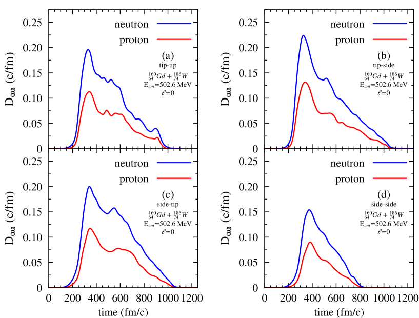
Figure 2: Neutron and proton diffusion coefficient in the head-on collision of ${}^{160}\text{Gd}+{}^{186}\text{W}$ system at $E_{\text{c.m.}}=502.6$ MeV in tip-tip (a), tip-side (b), side-tip (c) and side-side (d) collision geometries.

In the most general formulation, the diffusion coefficients are over a complete set of particle-hole states. In the diabatic limit we can get rid of the particle states by utilizing closure relations. As a consequence the diffusion coefficients are then obtained solely in terms of the occupied single-particle states of the TDHF calculations, which provides a significant simplification. Our previous publications provide all the explicit expressions for the diffusion coefficients [59, 60, 61, 62, 63, 64, 65, 66, 67]. The analysis of these coefficients are also provided in Appendix B in Ref. [59]. The determination of the diffusion coefficients by virtue of the mean-field properties is consistent with the fluctuation dissipation theorem of non-equilibrium statistical mechanics and it significantly uncomplicates the calculation of quantal diffusion coefficients. Quantal properties such as shell effects, Pauli principle, and the effect of the unrestricted collision geometry, are included in these diffusion coefficients without any adjustable parameters. We point out that there is a close analogy between the quantal expression and the classical diffusion coefficient for a random walk problem [68, 69, 70]. The direct part is given as the sum of the nucleon currents across the window from the projectile-like fragment to the target-like fragment and from the target-like fragment to the projectile-like fragment, integrated over the memory. This is analogous to the random walk problem, in which the diffusion coefficient is given by the sum of the rate of the forward and backward steps. Pauli blocking effects in the transfer mechanism does not have a classical counterpart and is represented in the second part of the quantal diffusion equations. This is illustrated in Fig. 2, where we plot the neutron and proton diffusion coefficients in head-on collisions of ${}^{160}\text{Gd}+{}^{186}\text{W}$ system at $E_{\text{c.m.}}=502.6$ MeV for different collision geometries.

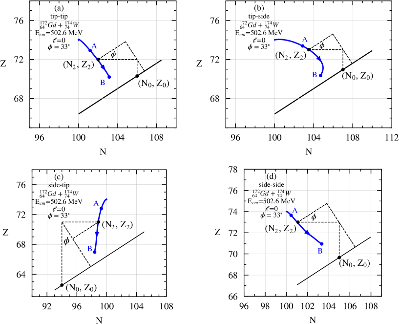
Figure 3: Blue curves show drift path of W-like fragments in the head-on collision of ${}^{172}\text{Gd}+{}^{174}\text{W}$ system at $E_{\text{c.m.}}=502.6$ MeV in tip-tip (a), tip-side (b), side-tip (c) and side-side (d) geometries.

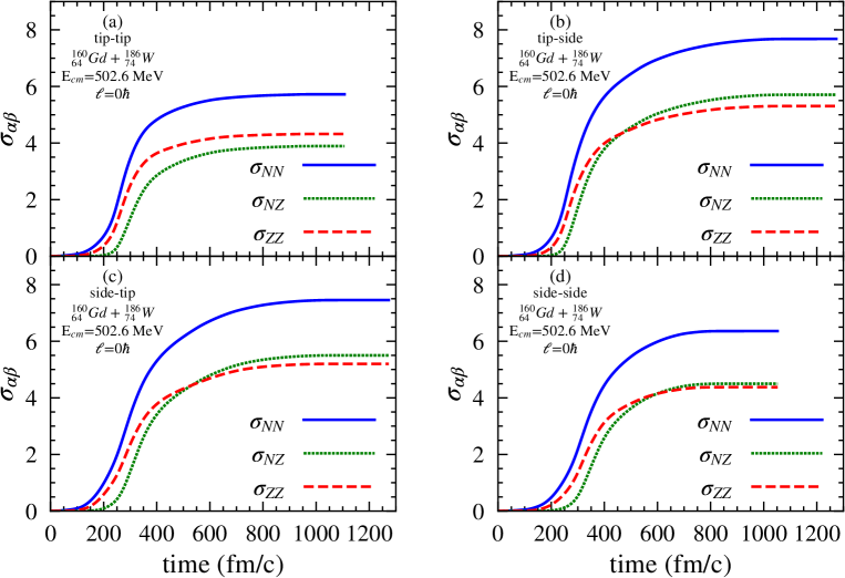
Figure 4: Neutron, proton and mixed variances as a function of time in the head-on collision of ${}^{160}\text{Gd}+{}^{186}\text{W}$ system at $E_{\text{c.m.}}=502.6$ MeV in tip-tip (a), tip-side (b), side-tip (c) and side-side (d) geometries.

III.3 Potential energy of di-nuclear system

Nucleon drift mechanism as well as dispersions of fragment distributions are determined in terms of two competing effects: (i) Nucleon diffusion tends to increase dispersion of distribution functions and (ii) Potential energy of di-nuclear system $U(N_{2},Z_{2})$ on neutron and proton plane that controls the mean nucleon drift and determines saturation values of dispersions. Potential energy of the di-nuclear system consists mainly of electrostatic energy, symmetry energy, surface energy, and centrifugal energy. The TDHF theory encompasses different energy contributions at the microscopic level. Furthermore, TDHF calculations illustrate potential energy depends on the geometry of di-nuclear system. It is possible to extract useful information about potential energy with the help of Einstein relation in the over damped limit [59, 60, 61, 62, 63]. In the over damped limit, drift coefficients are related to the potential energy surface in $(N,Z)$ plane as

$$v_{n}(t) =-\frac{D_{NN}(t)}{T^{*}}\frac{\partial}{\partial N_{2}}U(N_{2},Z_{2})\;,$$ (10a)

$$v_{z}(t) =-\frac{D_{ZZ}(t)}{T^{*}}\frac{\partial}{\partial Z_{2}}U(N_{2},Z_{2})\;,$$ (10b)

where $T^{\ast}$ stands for the effective temperature of the system, and $N_{2},Z_{2}$ indicate neutron-proton numbers of W-like fragments in the di-nuclear system. Drift information of ${}^{160}\text{Gd}+{}^{186}\text{W}$ system give information about potential energy only in the iso-scalar direction. To obtain information about potential energy in direction perpendicular to the stability valley, we consider collision of a neighboring system ${}^{172}\text{Gd}+{}^{174}\text{W}$ at $E_{\text{c.m.}}=502.6$ MeV. Fig. 3 shows drift path of W-like fragments in head-on collisions in different geometries. In all geometries, system rapidly follows a path nearly perpendicular direction to the stability valley to reach charge asymmetry equilibrium. We refer the direction perpendicular to stability valley as the iso-vector direction. Evolution in iso-vector direction is accompanied by drift along iso-scalar path toward symmetry or asymmetry. At the end of relatively short contact time, system separates before reaching the local equilibrium state.

In collisions of ${}^{160}\text{Gd}+{}^{186}\text{W}$ system, heavier local equilibrium state is in vicinity of lead valley with neutron and proton numbers around $N_{0}=124$, $Z_{0}=82$, while the lighter local equilibrium state is in the neighborhood of barium valley having neutron and proton numbers near $\overline{N_{0}}=84$, $\overline{Z_{0}}=56$. These nuclei are located on the iso-scalar path with the charge asymmetry 0.20. The drift information of these two similar systems, when combined, can provide an approximate description of potential energy surface of the di-nuclear system relative to the equilibrium value of potential energy in terms of two parabolic forms,

$$U(N_{2},Z_{2})=\frac{1}{2}aR_{S}^{2}(N_{2},Z_{2})+\frac{1}{2}bR_{V}^{2}(N_{2},Z_{2})\;.$$ (11)

Here, $R_{S}(N_{2},Z_{2})$ and $R_{V}(N_{2},Z_{2})$ represent perpendicular distances of a fragment with neutron and proton numbers $(N_{2},Z_{2})$ from the isoscalar path and from the local equilibrium state along the isoscalar path, respectively.

As a consequence of the sharp increase in asymmetry energy, we anticipate the isovector curvature parameter to be considerably greater than the corresponding isoscalar curvature parameter. From the geometry of Fig. 1 and Fig. 3, we express iso-vector and iso-scalar distances in terms of neutron and proton number of the fragment and neutron and proton numbers of equilibrium states. When drift is in asymmetry direction iso-scalar distance is given by $R_{V}(t)=\left[~{}N_{0}-N_{2}(t)~{}\right]\text{cos}\phi+\left[~{}Z_{0}-Z_{2}(t)~{}\right]\text{sin}\phi$, and for drift in symmetry direction it is given by $\overline{R_{V}}(t)=\left[~{}N_{2}(t)-\overline{N_{0}}~{}\right]\text{cos}\phi+\left[~{}Z_{2}(t)-\overline{Z_{0}}~{}\right]\text{sin}\phi$. In both cases iso-vector distance is given by $R_{S}(t)=\left[~{}N_{0}-N_{2}(t)~{}\right]\text{sin}\phi-\left[~{}Z_{0}-Z_{2}(t)~{}\right]\text{cos}\phi$. The angle $\phi$ is the angle between the iso-scalar path and $N$-axis which is about $\phi=33^{\circ}$.

Mean drift coefficients and diffusion coefficients are determined from the TDHF and SMF calculations, using Einstein relations in Eq. (10), we can determine the reduced curvature coefficients $\alpha=a/T^{\ast}$ and $\beta=b/T^{\ast}$. Only ratios of the curvature parameters and the effective temperature appear. As a result, the effective temperature is not a parameter in the description. The reduced curvature parameters in each collision geometry vary in time due the shell structure of TDHF description. In calculations of dispersion values we employ constant curvature parameters, which are determined by averaging over suitable time intervals when the overlap between the colliding nuclei are sufficiently large. When drift occurs toward asymmetry, the averaged value of the iso-scalar reduced curvature parameter over a time interval $t_{B}$ and $t_{C}$ is determined as,

$$\beta^{asym}=\frac{1}{R_{V}^{asym}}\int_{t_{B}}^{t_{C}}\left(\frac{v_{n}(t)\cos\phi}{D_{NN}(t)}+\frac{v_{p}(t)\sin\phi}{D_{ZZ}(t)}\right)dt\;,$$ (12)

where the integrated value of isoscalar distance for drift towards asymmetry is given by

$$R_{V}^{asym}=\int_{t_{B}}^{t_{C}}\left\{\left[~{}N_{0}-N_{2}(t)~{}\right]\text{cos}\phi+\left[~{}Z_{0}-Z_{2}(t)~{}\right]\text{sin}\phi\right\}dt\;.$$ (13)

When drift occurs toward symmetry, we can determine the averaged value of the iso-scalar reduced curvature parameter over a time interval $t_{A}$ and $t_{B}$ as,

$$\beta^{sym}=-\frac{1}{R_{V}^{sym}}\int_{t_{A}}^{t_{B}}\left(\frac{v_{n}(t)\cos\phi}{D_{NN}(t)}+\frac{v_{p}(t)\sin\phi}{D_{ZZ}(t)}\right)dt\;,$$ (14)

where the integrated value of isoscalar distance for drift towards symmetry is given by

$$R_{V}^{sym}=\int_{t_{A}}^{t_{B}}\left\{\left[~{}N_{2}(t)-\overline{N_{0}}~{}\right]\text{cos}\phi+\left[~{}Z_{2}(t)-\overline{Z_{0}}~{}\right]\text{sin}\phi\right\}dt\;.$$ (15)

Table 3: Calculation of $\beta$ curvature parameter using ${}^{160}\text{Gd}+{}^{186}\text{W}$ system at $E_{\text{c.m.}}=502.6$ MeV in tip-tip(XX), tip-side (XY), side-tip (YX) and side-side (YY) geometries. The time intervals $t_{A}$, $t_{B}$ and $t_{C}$ required to calculate isoscalar curvature parameters are shown in Fig. 1A.

${}^{160}\text{Gd}+{}^{186}\text{W}$	$t_{A}$	$t_{B}$	$t_{C}$	$\beta^{sym}_{AB}$	$\beta^{asym}_{BC}$	$\overline{\beta}=(\beta^{sym}_{AB}+\beta^{asym}_{BC})/2$
tip-tip	260	250	800	0.010	0.034	0.022
tip-side	—	250	900	—	0.008	0.008
side-tip	260	380	900	0.016	0.004	0.010
side-side	300	450	750	0.007	0.010	0.009

These expressions can be used to calculate the averaged values of isoscalar reduced curvature parameters in different geometries. In Table 3, the calculated values of isoscalar reduced curvature parameters for different geometries are given. In tip-tip, side-tip and side-side geometries, initially drift towards symmetry is observed, followed by a drift towards asymmetry. For these geometries, we determine the isoscalar curvature parameter by taking the average of drift towards symmetry and drift towards asymmetry part, given as $\overline{\beta}=(\beta^{sym}_{AB}+\beta^{asym}_{BC})/2$.

Table 4: Calculation of $\alpha$ curvature parameter using ${}^{172}\text{Gd}+{}^{174}\text{W}$ system at $E_{\text{c.m.}}=502.6$ MeV in tip-tip (XX), tip-side (XY), side-tip (YX) and side-side (YY) geometries. The time intervals $t_{A}$ and $t_{B}$ required to calculate isovector curvature parameters are shown in Fig. 2A.

${}^{172}\text{Gd}+{}^{174}\text{W}$	$t_{A}$	$t_{B}$	$\alpha$
tip-tip	180	260	0.113
tip-side	250	400	0.133
side-tip	200	350	0.127
side-side	250	450	0.143

We estimate the iso-vector reduced curvature parameters in different geometries from the drift paths of ${}^{172}\text{Gd}+{}^{174}\text{W}$ system at $E_{\text{c.m.}}=502.6$ MeV by averaging over time interval $t_{A}$ and $t_{B}$ as,

$$\alpha=\frac{1}{R_{S}}\int_{t_{A}}^{t_{B}}\left(\frac{v_{n}(t)\sin\phi}{D_{NN}(t)}-\frac{v_{p}(t)\cos\phi}{D_{ZZ}(t)}\right)dt\;,$$ (16)

where the integrated value of iso-vector distance is given by

$$R_{S}=\int_{t_{A}}^{t_{B}}\left\{\left[~{}N_{0}-N_{2}(t)~{}\right]\text{sin}\phi-\left[~{}Z_{0}-Z_{2}(t)~{}\right]\text{cos}\phi\right\}dt\;.$$ (17)

In Eq. (16), diffusion coefficients for ${}^{172}\text{Gd}+{}^{174}\text{W}$ system at $E_{\text{c.m.}}=502.6$ MeV are plotted in Fig. 3A.

We can use these expressions in calculating averaged values of isovector reduced curvature parameters in different geometries. In Table 4, the calculated values of isovector reduced curvature parameters for different geometries are given.

Potential energy surface in (N-Z) plane should not depend on the centrifugal potential energy and excitation energy of the di-nuclear system. Therefore, in ${}^{160}\text{Gd}+{}^{186}\text{W}$ system at $E_{\text{c.m.}}=461.9$ MeV, we employ the same curvature parameters which are determined at $E_{\text{c.m.}}=502.6$ MeV. Since the drift coefficients have analytical form, we can immediately determine their derivatives to find,

$$\frac{\partial\nu_{n}}{\partial N_{2}} =-D_{NN}\left(\alpha\sin^{2}\phi+\beta\cos^{2}\phi\right)\;,$$ (18)

$$\frac{\partial\nu_{z}}{\partial Z_{2}} =-D_{ZZ}\left(\alpha\cos^{2}\phi+\beta\sin^{2}\phi\right)\;,$$ (19)

$$\frac{\partial\nu_{n}}{\partial Z_{2}} =-D_{NN}\left(\beta-\alpha\right)\sin\phi\cos\phi\;,$$ (20)

$$\frac{\partial\nu_{z}}{\partial N_{2}} =-D_{ZZ}\left(\beta-\alpha\right)\sin\phi\cos\phi\;.$$ (21)

The curvature parameter $\alpha$ perpendicular to the beta stability valley is much larger than the curvature parameter $\beta$ along the stability valley. Consequently, $\beta$ does not have an appreciable effect on the derivatives of the drift coefficients. These derivative expressions are needed to calculate neutron, proton, and mixed dispersions, as discussed in the following section.

III.4 Fragment Probability Distributions

In general, the combined probability distribution function $P_{\ell}(N,Z)$ for producing a fragment with neutron $N$ and proton $Z$ is obtained by producing a large number of solutions of Langevin Eq. (5). The equivalence between the Langevin Equation and the Fokker-Planck equation, for the distribution function of the macroscopic variables [69], is of common knowledge. When the drift coefficients are linear functions of macroscopic variables, as in the case of Eq. (5), the proton and neutron distribution function for initial angular momentum $\ell$ is given as a correlated Gaussian function described by the mean values, and the neutron, proton, and mixed dispersion, as

$$P_{\ell}(N,Z)=\frac{1}{2\pi\sigma_{NN}(\ell)\sigma_{ZZ}(\ell)\sqrt{1-\rho_{\ell}^{2}}}\exp\left(-C_{\ell}\right)\;.$$ (22)

Here, the exponent $C_{\ell}$ is given by

$$C_{\ell}=\frac{1}{2\left(1-\rho_{\ell}^{2}\right)} \left[\left(\frac{Z-Z_{\ell}}{\sigma_{ZZ}(\ell)}\right)^{2}-2\rho_{\ell}\left(\frac{Z-Z_{\ell}}{\sigma_{ZZ}(\ell)}\right)\left(\frac{N-N_{\ell}}{\sigma_{NN}(\ell)}\right)\right.$$

$$\left.+\left(\frac{N-N_{\ell}}{\sigma_{NN}(\ell)}\right)^{2}\right]\;,$$ (23)

with the correlation coefficient defined as $\rho_{\ell}=\sigma_{\text{NZ}}^{2}(\ell)/(\sigma_{\text{ZZ}}(\ell)\sigma_{\text{NN}}(\ell))$. Quantities $N_{\ell}=\overline{N}_{\ell}^{\lambda}$, $Z_{\ell}=\overline{Z}_{\ell}^{\lambda}$ denote the mean neutron and proton numbers of the target-like or project-like fragments. These mean values are obtained by performing TDHF calculations. It is possible to deduce coupled differential equations for variances $\sigma_{\text{NN}}^{2}(\ell)=\overline{\mathit{\delta N}^{\lambda}\mathit{\delta N}^{\lambda}}$, $\sigma_{\text{ZZ}}^{2}(\ell)=\overline{\mathit{\delta Z}^{\lambda}\mathit{\delta Z}^{\lambda}}$, and co-variances $\sigma_{\text{NZ}}^{2}(\ell)=\overline{\mathit{\delta N}^{\lambda}\mathit{\delta Z}^{\lambda}}$ by multiplying Langevin Eq. (5) with $\mathit{\delta N}^{\lambda}$, ${\delta Z}^{\lambda}$ and carrying out the average over the ensemble generated from the solution of the Langevin equation. These coupled equations were obtained in Refs. [59, 60, 61, 62, 71, 63, 64]. We provide these differential equations here again for completeness [72],

$$\frac{\partial}{\partial t}{\sigma}^{2}_{NN}=2\frac{\partial\nu_{n}}{\partial N_{2}}\sigma^{2}_{NN}+2\frac{\partial\nu_{n}}{\partial Z_{2}}\sigma^{2}_{NZ}+2D_{NN}\;,$$ (24)

$$\frac{\partial}{\partial t}{\sigma}^{2}_{ZZ}=2\frac{\partial\nu_{p}}{\partial Z_{2}}\sigma^{2}_{ZZ}+2\frac{\partial\nu_{p}}{\partial N_{2}}\sigma^{2}_{NZ}+2D_{ZZ}\;,$$ (25)

and

$$\frac{\partial}{\partial t}{\sigma}^{2}_{NZ}=\frac{\partial\nu_{p}}{\partial N_{1}}\sigma^{2}_{NN}+\frac{\partial\nu_{n}}{\partial Z_{1}}\sigma^{2}_{ZZ}+\sigma^{2}_{NZ}\left(\frac{\partial\nu_{p}}{\partial Z_{2}}+\frac{\partial\nu_{n}}{\partial N_{2}}\right).$$ (26)

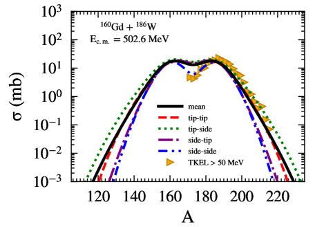
Figure 5: Total cross-section in collision of ${}^{160}\text{Gd}+{}^{186}\text{W}$ system at $E_{\text{c.m.}}=502.6$ MeV as a function of mass number A. Different geometries are indicated by dashed (red), dotted (green), dashed-dotted (brown) and dashed-dot-dotted (blue) lines. Average cross-section and experimental data taken from Ref. [52] are indicated by solid black line and yellow triangles respectively.

The set of coupled equations are also familiar from the phenomenological nucleon exchange model, and they were derived from the Fokker-Planck equation for the fragment neutron and proton distributions in the deep-inelastic heavy-ion collisions  [70, 72]. Variances and co-variances are determined from the solutions of these coupled differential equations with initial conditions $\sigma^{2}_{NN}(t=0)=0$, $\sigma^{2}_{ZZ}(t=0)=0$ and $\sigma^{2}_{NZ}(t=0)=0$ for each angular momentum $\ell$. As an example, Fig. 4 shows neutron, proton dispersions, and mix dispersions in collision of ${}^{160}\text{Gd}+{}^{186}\text{W}$ with initial angular momentum $\ell=0\hbar$ at $E_{\text{c.m.}}=502.6$ MeV for different geometries. Probability distribution of mass number of produced fragments is determined by summing over N or Z and keeping the total mass number constant $A=N+Z$.

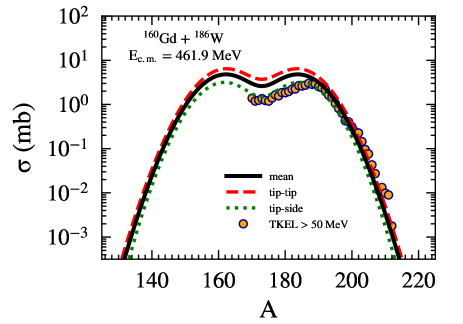
Figure 6: Total cross-section in collision of ${}^{160}\text{Gd}+{}^{186}\text{W}$ system at $E_{\text{c.m.}}=461.9$ MeV as a function of mass number A. Different geometries are indicated by dotted (green), dashed (red) lines. Average cross-section and experimental data taken from Ref. [52] are indicated by solid black line and yellow circles respectively.

$$P_{\ell}(A)=\frac{1}{\sqrt{2\pi}\sigma_{AA}}\exp\left[\frac{-1}{2}\left(\frac{A-A_{\ell}}{\sigma_{AA}(\ell)}\right)^{2}\right]\ ,$$ (27)

where mass variance is given by $\sigma_{AA}^{2}=\sigma_{NN}^{2}+\sigma_{ZZ}^{2}+2\sigma_{NZ}^{2}.$

IV Production cross-sections of primary fragments

It is possible to calculate double cross-sections as a function of neutron and proton numbers of primary fragments. In experimental analysis of Kozulin et al. [52], only mass distribution of primary fragments is published. Therefore, we present calculation of cross-sections $\sigma^{s}(A)$ as function of mass number A of primary fragments using the familiar expression,

$$\sigma^{s}(A)=\frac{\pi\hbar^{2}}{2{\mu}E_{\text{c.m.}}}\sum\limits_{\ell_{min}}^{\ell_{max}}(2\ell+1)P^{s}_{\ell}(A)\,$$ (28)

with

$$P_{\ell}^{s}(A)=\frac{1}{2}[P_{\ell,pro}^{s}(A)+P_{\ell,tar}^{s}(A)]\;.$$ (29)

Here label “s” indicates the different geometries of collision. In this expression, $P_{\ell,pro}^{s}(A)$ and $P_{\ell,tar}^{s}(A)$ denotes the normalized probability of producing projectile-like and target-like fragments. These probabilities are given by Eq. (27) with mean values are projectile-like and target-like fragments, respectively. To make the total primary fragment distribution normalized to unity we multiply by a factor $1/2$. In summation over initial angular momentum $\ell$, the range of initial orbital angular momentum depends on the geometry of the detectors in the laboratory frame. In calculations, we carry out summation over the range from $\ell_{\text{min}}$ to $\ell_{\text{max}}$. The range of $\ell$-values are specified by the angular acceptance of the detector. In laboratory frame, the range of acceptance of detector is $25^{\circ}-65^{\circ}$. The range of $\ell$-values for different geometries are indicated in Table 1 at $E_{\text{c.m.}}=502.6$ MeV and Table  2 at $E_{\text{c.m.}}=461.9$ MeV. For $E_{\text{c.m.}}=461.9$ MeV energy, there are no $\ell$-value in side-tip and side-side geometries leading to acceptance range of detector. Fig. 5 shows cross-sections at $E_{\text{c.m.}}=502.6$ MeV as a function of mass number A for production of primary fragments in tip-tip, tip-side, side-tip and side-side geometries with different colors. Average values of the cross-sections are determined by the arithmetic mean values $\overline{\sigma}(A)=\frac{1}{4}\sum\limits_{s}\sigma^{s}(A)$ of cross-sections at different geometries. Fig. 6 shows total cross-sections at $E_{\text{c.m.}}=461.9$ MeV energy as a function of mass number A for production of primary fragments in tip-tip and tip-side geometries with different colors. Cross-sections in side-tip, and side-side geometries are nearly zero, and not indicated in the figure. Total cross-section is essentially determined by tip-tip and tip-side contributions. In this case, average values of the cross-sections are determined by the arithmetic mean values of tip-tip and tip-side contributions, $\overline{\sigma}(A)=\frac{1}{2}\sum\limits_{s}\sigma^{s}(A)$ Calculations provide good descriptions of measurements that are indicated by yellow triangles at high energy data and by yellow circles at low energy data.

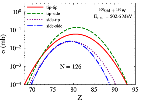
Figure 7: Primary product cross sections for $N=126$ isotones in collision of ${}^{160}\text{Gd}+{}^{186}\text{W}$ system at $E_{\text{c.m.}}=502.6$ MeV are shown as a function of the proton number of the reaction products. Different geometries are indicated by solid (red), dotted (green), dotted (purple) and dashed-dotted (blue) lines.

Finally, the prediction of primary production cross sections for $N=126$ isotones in the ${}^{160}\text{Gd}+{}^{186}\text{W}$ system at $E_{\text{c.m.}}=502.6$ MeV are given in Fig. 7. It is observed that the primary product cross sections in the tip-side geometry are roughly one order of magnitude higher than those in the side-tip and side-side geometries, highlighting the effect of inverse quasi-fission observed in the tip-side geometry. Results clearly demonstrate that depending on the deformation and relative orientation of the reaction partners, outcome of the reaction differs. This effect supports the idea that MNT reactions can serve as a useful tool to produce neutron rich heavy nuclei near the lead region, which may not be available via fusion-fission and fragmentation.

V Conclusions

We investigate multi-nucleon transfer mechanism in quasi-fission reactions of ${}^{160}\text{Gd}+{}^{186}\text{W}$ system at $E_{\text{c.m.}}=502.6$ MeV and $E_{\text{c.m.}}=461.9$ MeV employing quantal diffusion description based on the Stochastic Mean-Field approach. We evaluate transport coefficients associated with charge and mass asymmetry variables in terms of time-dependent single-particle wave functions of TDHF theory. Transport description includes quantal effect due to shell structure, full geometry of the collision dynamics and Pauli Exclusion Principle and does not involve any adjustable parameters aside from the standard description of the effective Hamiltonian of TDHF theory. In transport description, in addition to diffusion coefficient, we need to determine first and second derivatives of the potential energy surface with respect to neutron and proton numbers. It is possible to determine iso-scalar and iso-vector curvature parameters in terms neutron and proton drift coefficients and diffusion coefficients with the help of Einstein relations. Joint probability distribution of primary fragments is determined by a correlated Gaussian function in terms of mean values of neutron-proton numbers and neutron, proton, mixed dispersions for each initial angular momentum. We calculate cross-sections of primary fragments as a function of mass number and compare with data of Kozulin et al. [52]. Calculations provide good description of primary mass distributions at both bombarding energies.

*

APPENDIX A A

We can estimate the averaged values of reduced isoscalar and isovector curvature parameters with the help of Einstein relations, Eq. (10), in the overdamped limit. We evaluate the average values of the reduced curvature parameters for different geometries by carrying out the time integrals in Eqs. (12-17) over suitable time intervals. These time intervals are indicated in following figures for ${}^{160}\text{Gd}+^{186}\text{W}$ and ${}^{172}\text{Gd}+^{174}\text{W}$ reactions at $E_{\text{c.m.}}=502.6$ MeV.

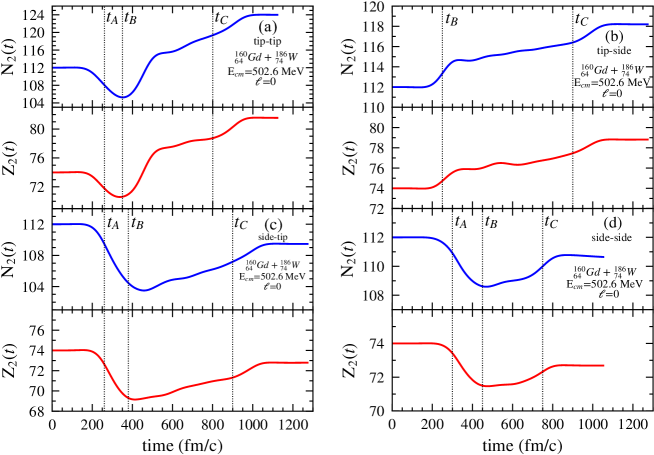
Figure 1A: Mean-values of neutron and proton numbers of W-like fragments in the head-on collision of ${}^{160}\mathrm{Gd}+{}^{186}\mathrm{W}$ system at $E_{\mathrm{c.m.}}=502.6$ MeV in tip-tip (a), tip-side (b), side-tip (c) and side-side (d) geometries.

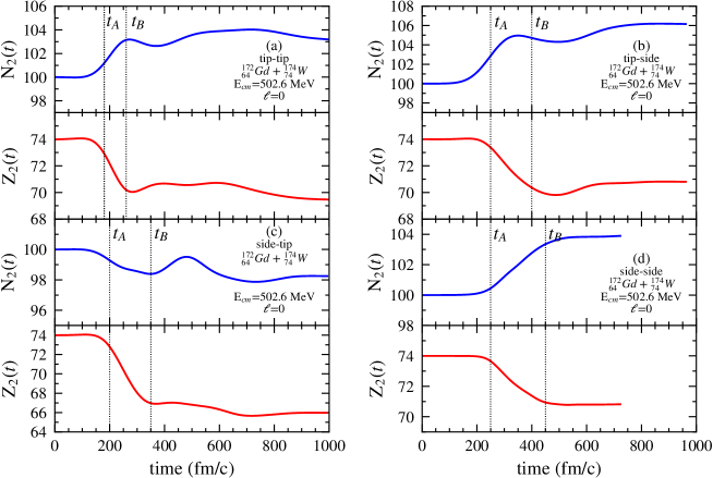
Figure 2A: Mean-values of neutron and proton numbers of W-like fragments in the head-on collision of ${}^{172}\text{Gd}+{}^{174}\text{W}$ system at $E_{\text{c.m.}}=502.6$ MeV in tip-tip (a), tip-side (b), side-tip (c) and side-side (d) geometries.

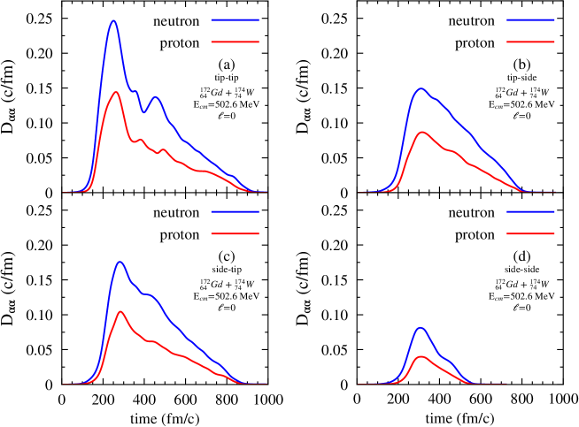
Figure 3A: Diffusion coefficients in the head-on collision of ${}^{172}\text{Gd}+{}^{174}\text{W}$ system at $E_{\text{c.m.}}=502.6$ MeV in tip-tip (a), tip-side (b), side-tip (c) and side-side (d) geometries.

References

- Chatillon et al. [2006] A. Chatillon, Ch. Theisen, P. T. Greenlees, G. Auger, J. E. Bastin, E. Bouchez, B. Bouriquet, J. M. Casandjian, R. Cee, E. Clément, R. Dayras, G. de France, R. de Toureil, S. Eeckhaudt, A. Göergen, T. Grahn, S. Grévy, K. Hauschild, R.-D. Herzberg, P. J. C. Ikin, G. D. Jones, P. Jones, R. Julin, S. Juutinen, H. Kettunen, A. Korichi, W. Korten, Y. Le Coz, M. Leino, A. Lopez-Martens, S. M. Lukyanov, Yu. E. Penionzhkevich, J. Perkowski, A. Pritchard, P. Rahkila, M. Rejmund, J. Saren, C. Scholey, S. Siem, M. G. Saint-Laurent, C. Simenel, Yu. G. Sobolev, Ch. Stodel, J. Uusitalo, A. Villari, M. Bender, P. Bonche, and P.-H. Heenen, Spectroscopy and single-particle structure of the odd-Z heavy elements 255Lr, 251Md and 247Es, Eur. Phys. J. A 30, 397 (2006).
- Herzberg et al. [2001] R.-D. Herzberg, P. T. Greenlees, P. A. Butler, G. D. Jones, M. Venhart, I. G. Darby, S. Eeckhaudt, K. Eskola, T. Grahn, C. Gray-Jones, F. P. Heßberger, P. Jones, R. Julin, S. Juutinen, S. Ketelhut, W. Korten, M. Leino, A.-P. Leppanen, S. Moon, M. Nyman, R. D. Page, J. Pakarinen, A. Pritchard, P. Rahkila, J. Saren, C. Scholey, A. Steer, Y. Sun, Ch. Theisen, and J. Uusitalo, Nuclear isomers in superheavy elements as stepping stones towards the island of stability, Nature 442, 896 (2001).
- Kozulin et al. [2012] E. M. Kozulin, E. Vardaci, G. N. Knyazheva, A. A. Bogachev, S. N. Dmitriev, I. M. Itkis, M. G. Itkis, A. G. Knyazev, T. A. Loktev, K. V. Novikov, E. A. Razinkov, O. V. Rudakov, S. V. Smirnov, W. Trzaska, and V. I. Zagrebaev, Mass distributions of the system at laboratory energies around the Coulomb barrier: A candidate reaction for the production of neutron–rich nuclei at , Phys. Rev. C 86, 044611 (2012).
- Kratz et al. [2013] J. V. Kratz, M. Schädel, and H. W. Gäggeler, Reexamining the heavy-ion reactions and and actinide production close to the barrier, Phys. Rev. C 88, 054615 (2013).
- Watanabe et al. [2015] Y. X. Watanabe, Y. H. Kim, S. C. Jeong, Y. Hirayama, N. Imai, H. Ishiyama, H. S. Jung, H. Miyatake, S. Choi, J. S. Song, E. Clement, G. de France, A. Navin, M. Rejmund, C. Schmitt, G. Pollarolo, L. Corradi, E. Fioretto, D. Montanari, M. Niikura, D. Suzuki, H. Nishibata, and J. Takatsu, Pathway for the Production of Neutron–Rich Isotopes around the Shell Closure, Phys. Rev. Lett. 115, 172503 (2015).
- Desai et al. [2019] V. V. Desai, W. Loveland, K. McCaleb, R. Yanez, G. Lane, S. S. Hota, M. W. Reed, H. Watanabe, S. Zhu, K. Auranen, A. D. Ayangeakaa, M. P. Carpenter, J. P. Greene, F. G. Kondev, D. Seweryniak, R. V. F. Janssens, and P. A. Copp, The reaction: A test of models of multi-nucleon transfer reactions, Phys. Rev. C 99, 044604 (2019).
- Adamian et al. [2010a] G. G. Adamian, N. V. Antonenko, V. V. Sargsyan, and W. Scheid, Possibility of production of neutron-rich Zn and Ge isotopes in multinucleon transfer reactions at low energies, Phys. Rev. C 81, 024604 (2010a).
- Adamian et al. [2010b] G. G. Adamian, N. V. Antonenko, and D. Lacroix, Production of neutron-rich Ca, Sn, and Xe isotopes in transfer-type reactions with radioactive beams, Phys. Rev. C 82, 064611 (2010b).
- Jiang and Wang [2020] X. Jiang and N. Wang, Probing the production mechanism of neutron-rich nuclei in multinucleon transfer reactions, Phys. Rev. C 101, 014604 (2020).
- Adamian et al. [2020] G. G. Adamian, N. V. Antonenko, A. Diaz-Torres, and S. Heinz, How to extend the chart of nuclides?, Eur. Phys. J. A 56, 47 (2020).
- Kalandarov et al. [2020] S. A. Kalandarov, G. G. Adamian, N. V. Antonenko, H. M. Devaraja, and S. Heinz, Production of neutron deficient isotopes in the multinucleon transfer reaction , Phys. Rev. C 102, 024612 (2020).
- Li et al. [2020] C. Li, J. Tian, and F. Zhang, Production mechanism of the neutron-rich nuclei in multinucleon transfer reactions: A reaction time scale analysis in energy dissipation process, Phys. Lett. B , 135697 (2020).
- Adamian et al. [2021] G. G. Adamian, N. V. Antonenko, H. Lenske, L. A. Malov, and S. Zhou, Self-consistent methods for structure and production of heavy and superheavy nuclei, Eur. Phys. J. A 57, 89 (2021).
- Itkis, M. G. et al. [2022] Itkis, M. G., Knyazheva, G. N., Itkis, I. M., and Kozulin, E. M., Experimental investigation of cross sections for the production of heavy and superheavy nuclei, Eur. Phys. J. A 58, 178 (2022).
- Heinz, S. and Devaraja, H. M. [2022] Heinz, S. and Devaraja, H. M., Nucleosynthesis in multinucleon transfer reactions, Eur. Phys. J. A 58, 114 (2022).
- Wu et al. [2022] Z. Wu, L. Guo, Z. Liu, and G. Peng, Production of proton-rich nuclei in the vicinity of via multinucleon transfer reactions, Phys. Lett. B 825, 136886 (2022).
- Hofmann and Münzenberg [2000] S. Hofmann and G. Münzenberg, The discovery of the heaviest elements, Rev. Mod. Phys. 72, 733 (2000).
- Oganessian et al. [2006] Yu. Ts. Oganessian, V. K. Utyonkov, Yu. V. Lobanov, F. Sh. Abdullin, A. N. Polyakov, R. N. Sagaidak, I. V. Shirokovsky, Yu. S. Tsyganov, A. A. Voinov, G. G. Gulbekian, S. L. Bogomolov, B. N. Gikal, A. N. Mezentsev, S. Iliev, V. G. Subbotin, A. M. Sukhov, K. Subotic, V. I. Zagrebaev, G. K. Vostokin, M. G. Itkis, K. J. Moody, J. B. Patin, D. A. Shaughnessy, M. A. Stoyer, N. J. Stoyer, P. A. Wilk, J. M. Kenneally, J. H. Landrum, J. F. Wild, and R. W. Lougheed, Synthesis of the isotopes of elements 118 and 116 in the and fusion reactions, Phys. Rev. C 74, 044602 (2006).
- Zagrebaev et al. [2006] V. I. Zagrebaev, Yu. Ts. Oganessian, M. G. Itkis, and W. Greiner, Superheavy nuclei and quasi-atoms produced in collisions of transuranium ions, Phys. Rev. C 73, 031602(R) (2006).
- Valery Zagrebaev and Walter Greiner [2008a] Valery Zagrebaev and Walter Greiner, New way for the production of heavy neutron-rich nuclei, J. Phys. G: Nucl. Part. Phys. 35, 125103 (2008a).
- Valery Zagrebaev and Walter Greiner [2008b] Valery Zagrebaev and Walter Greiner, Production of New Heavy Isotopes in Low–Energy Multinucleon Transfer Reactions, Phys. Rev. Lett. 101, 122701 (2008b).
- Zagrebaev and Greiner [2011] V. I. Zagrebaev and W. Greiner, Production of heavy and superheavy neutron-rich nuclei in transfer reactions, Phys. Rev. C 83, 044618 (2011).
- Karpov and Saiko [2017] A. V. Karpov and V. V. Saiko, Modeling near-barrier collisions of heavy ions based on a Langevin-type approach, Phys. Rev. C 96, 024618 (2017).
- Saiko and Karpov [2019] V. V. Saiko and A. V. Karpov, Analysis of multinucleon transfer reactions with spherical and statically deformed nuclei using a Langevin-type approach, Phys. Rev. C 99, 014613 (2019).
- Saiko and Karpov [2022] V. Saiko and A. Karpov, Multinucleon transfer as a method for production of new heavy neutron-enriched isotopes of transuranium elements, Eur. Phys. J. A 58, 41 (2022).
- Zhao-Qing Feng et al. [2009] Zhao-Qing Feng, Gen-Ming Jin, Jun-Qing Li, and Werner Scheid, Production of heavy and superheavy nuclei in massive fusion reactions, Nucl. Phys. A 816, 33 (2009).
- Feng et al. [2009] Z.-Q. Feng, G.-M. Jin, and J.-Q. Li, Production of heavy isotopes in transfer reactions by collisions of , Phys. Rev. C 80, 067601 (2009).
- Feng [2017] Z.-Q. Feng, Production of neutron–rich isotopes around in multinucleon transfer reactions, Phys. Rev. C 95, 024615 (2017).
- Zhao et al. [2009] K. Zhao, X. Wu, and Z. Li, Quantum molecular dynamics study of the mass distribution of products in MeV collisions, Phys. Rev. C 80, 054607 (2009).
- Zhao et al. [2016] K. Zhao, Z. Li, Y. Zhang, N. Wang, Q. Li, C. Shen, Y. Wang, and X. Wu, Production of unknown neutron–rich isotopes in collisions at near–barrier energy, Phys. Rev. C 94, 024601 (2016).
- Wang and Guo [2016] N. Wang and L. Guo, New neutron-rich isotope production in , Phys. Lett. B 760, 236 (2016).
- Simenel [2012] C. Simenel, Nuclear quantum many-body dynamics, Eur. Phys. J. A 48, 152 (2012).
- Simenel and Umar [2018] C. Simenel and A. S. Umar, Heavy-ion collisions and fission dynamics with the time–dependent Hartree-Fock theory and its extensions, Prog. Part. Nucl. Phys. 103, 19 (2018).
- Nakatsukasa et al. [2016] T. Nakatsukasa, K. Matsuyanagi, M. Matsuo, and K. Yabana, Time-dependent density-functional description of nuclear dynamics, Rev. Mod. Phys. 88, 045004 (2016).
- Oberacker et al. [2014] V. E. Oberacker, A. S. Umar, and C. Simenel, Dissipative dynamics in quasifission, Phys. Rev. C 90, 054605 (2014).
- Umar et al. [2015] A. S. Umar, V. E. Oberacker, and C. Simenel, Shape evolution and collective dynamics of quasifission in the time-dependent Hartree-Fock approach, Phys. Rev. C 92, 024621 (2015).
- Umar and Oberacker [2015] A. S. Umar and V. E. Oberacker, Time-dependent HF approach to SHE dynamics, Nucl. Phys. A 944, 238 (2015).
- Umar et al. [2017] A. S. Umar, C. Simenel, and W. Ye, Transport properties of isospin asymmetric nuclear matter using the time-dependent Hartree–Fock method, Phys. Rev. C 96, 024625 (2017).
- Simenel [2010] C. Simenel, Particle Transfer Reactions with the Time-Dependent Hartree-Fock Theory Using a Particle Number Projection Technique, Phys. Rev. Lett. 105, 192701 (2010).
- Sekizawa and Yabana [2016] K. Sekizawa and K. Yabana, Time-dependent Hartree-Fock calculations for multinucleon transfer and quasifission processes in the reaction, Phys. Rev. C 93, 054616 (2016).
- Kazuyuki Sekizawa [2019] Kazuyuki Sekizawa, TDHF Theory and Its Extensions for the Multinucleon Transfer Reaction: A Mini Review, Front. Phys. 7, 20 (2019).
- Tohyama and Umar [2002] M. Tohyama and A. S. Umar, Quadrupole resonances in unstable oxygen isotopes in time-dependent density-matrix formalism, Phys. Lett. B 549, 72 (2002).
- Tohyama [2020] M. Tohyama, Applications of Time-Dependent Density-Matrix Approach, Front. Phys. 8, 67 (2020).
- Simenel [2011] C. Simenel, Particle-Number Fluctuations and Correlations in Transfer Reactions Obtained Using the Balian-Vénéroni Variational Principle, Phys. Rev. Lett. 106, 112502 (2011).
- Ayik [2008] S. Ayik, A stochastic mean-field approach for nuclear dynamics, Phys. Lett. B 658, 174 (2008).
- Lacroix and Ayik [2014] D. Lacroix and S. Ayik, Stochastic quantum dynamics beyond mean field, Eur. Phys. J. A 50, 95 (2014).
- Balian and Vénéroni [1985] R. Balian and M. Vénéroni, Time-dependent variational principle for the expectation value of an observable: Mean-field applications, Ann. Phys. (NY) 164, 334 (1985).
- Balian and Vénéroni [1992] R. Balian and M. Vénéroni, Correlations and fluctuations in static and dynamic mean-field approaches, Ann. Phys. 216, 351 (1992).
- Williams et al. [2018] E. Williams, K. Sekizawa, D. J. Hinde, C. Simenel, M. Dasgupta, I. P. Carter, K. J. Cook, D. Y. Jeung, S. D. McNeil, C. S. Palshetkar, D. C. Rafferty, K. Ramachandran, and A. Wakhle, Exploring Zeptosecond Quantum Equilibration Dynamics: From Deep-Inelastic to Fusion-Fission Outcomes in Reactions, Phys. Rev. Lett. 120, 022501 (2018).
- Godbey and Umar [2020] K. Godbey and A. S. Umar, Quasifission Dynamics in Microscopic Theories, Front. Phys. 8, 40 (2020).
- Godbey et al. [2020] K. Godbey, C. Simenel, and A. S. Umar, Microscopic predictions for the production of neutron-rich nuclei in the reaction , Phys. Rev. C 101, 034602 (2020).
- Kozulin et al. [2017] E. M. Kozulin, V. I. Zagrebaev, G. N. Knyazheva, I. M. Itkis, K. V. Novikov, M. G. Itkis, S. N. Dmitriev, I. M. Harca, A. E. Bondarchenko, A. V. Karpov, V. V. Saiko, and E. Vardaci, Inverse quasifission in the reactions , Phys. Rev. C 96, 064621 (2017).
- Washiyama and Lacroix [2009] K. Washiyama and D. Lacroix, Energy dissipation in fusion reactions from dynamical mean-field theory, Int. J. Mod. Phys. E 18, 2114 (2009).
- Reinhard et al. [1988] P.-G. Reinhard, A. S. Umar, K. T. R. Davies, M. R. Strayer, and S.-J. Lee, Dissipation and forces in time-dependent Hartree-Fock calculations, Phys. Rev. C 37, 1026 (1988).
- David J. Kedziora and Cédric Simenel [2010] David J. Kedziora and Cédric Simenel, New inverse quasifission mechanism to produce neutron-rich transfermium nuclei, Phys. Rev. C 81, 044613 (2010).
- Umar et al. [1991] A. S. Umar, M. R. Strayer, J. S. Wu, D. J. Dean, and M. C. Güçlü, Nuclear Hartree-Fock calculations with splines, Phys. Rev. C 44, 2512 (1991).
- Umar and Oberacker [2006] A. S. Umar and V. E. Oberacker, Three-dimensional unrestricted time-dependent Hartree-Fock fusion calculations using the full Skyrme interaction, Phys. Rev. C 73, 054607 (2006).
- Ka–Hae Kim et al. [1997] Ka–Hae Kim, Takaharu Otsuka, and Paul Bonche, Three-dimensional TDHF calculations for reactions of unstable nuclei, J. Phys. G: Nucl. Part. Phys. 23, 1267 (1997).
- Ayik et al. [2017] S. Ayik, B. Yilmaz, O. Yilmaz, A. S. Umar, and G. Turan, Multinucleon transfer in central collisions of , Phys. Rev. C 96, 024611 (2017).
- Ayik et al. [2018] S. Ayik, B. Yilmaz, O. Yilmaz, and A. S. Umar, Quantal diffusion description of multinucleon transfers in heavy–ion collisions, Phys. Rev. C 97, 054618 (2018).
- Yilmaz et al. [2018] B. Yilmaz, S. Ayik, O. Yilmaz, and A. S. Umar, Multinucleon transfer in and in a stochastic mean-field approach, Phys. Rev. C 98, 034604 (2018).
- Ayik et al. [2019a] S. Ayik, B. Yilmaz, O. Yilmaz, and A. S. Umar, Quantal diffusion approach for multinucleon transfers in collisions, Phys. Rev. C 100, 014609 (2019a).
- Sekizawa and Ayik [2020] K. Sekizawa and S. Ayik, Quantal diffusion approach for multinucleon transfer processes in the reactions: Toward the production of unknown neutron-rich nuclei, Phys. Rev. C 102, 014620 (2020).
- Ayik and Sekizawa [2020] S. Ayik and K. Sekizawa, Kinetic-energy dissipation and fluctuations in strongly damped heavy-ion collisions within the stochastic mean-field approach, Phys. Rev. C 102, 064619 (2020).
- Yilmaz et al. [2020] O. Yilmaz, G. Turan, and B. Yilmaz, Quasi-fission and fusion-fission reactions in collisions at MeV, Eur. Phys. J. A 56, 37 (2020).
- Ayik et al. [2020] S. Ayik, B. Yilmaz, O. Yilmaz, and A. S. Umar, Merging of transport theory with the time-dependent Hartree-Fock approach: Multinucleon transfer in collisions, Phys. Rev. C 102, 024619 (2020).
- Ayik et al. [2023] S. Ayik, M. Arik, O. Yilmaz, B. Yilmaz, and A. S. Umar, Multinucleon transfer mechanism in collisions using the quantal transport description based on the stochastic mean-field approach, Phys. Rev. C 107, 014609 (2023).
- Gardiner [1991] C. W. Gardiner, Quantum Noise (Springer–Verlag, Berlin, 1991).
- Weiss [1999] U. Weiss, Quantum Dissipative Systems, 2nd ed. (World Scientific, Singapore, 1999).
- Hannes Risken and Till Frank [1996] Hannes Risken and Till Frank, The Fokker–Planck Equation (Springer–Verlag, Berlin, 1996).
- Ayik et al. [2019b] S. Ayik, O. Yilmaz, B. Yilmaz, and A. S. Umar, Heavy-isotope production in collisions at MeV, Phys. Rev. C 100, 044614 (2019b).
- Schröder et al. [1981] W. U. Schröder, J. R. Huizenga, and J. Randrup, Correlated mass and charge transport induced by statistical nucleon exchange in damped nuclear reactions, Phys. Lett. B 98, 355 (1981).