Diverse universality classes of the topological deconfinement transitions
of three-dimensional noncompact lattice Abelian Higgs models

Abstract

We study the topological phase transitions occurring in three-dimensional (3D) multicomponent lattice Abelian Higgs (LAH) models, in which an $N$-component scalar field is minimally coupled with a noncompact Abelian gauge field, with a global $SU(N)$ symmetry. Their phase diagram presents a high-temperature Coulomb (C) phase, and two low-temperature molecular (M) and Higgs (H) phases, both characterized by the spontaneous breaking of the $SU(N)$ symmetry. The molecular-Higgs (MH) and Coulomb-Higgs (CH) transitions are topological transitions, separating a phase with gapless gauge modes and confined charges from a phase with gapped gauge modes and deconfined charged excitations. These transitions are not described by effective Landau-Ginzburg-Wilson theories, due to the active role of the gauge modes. We show that the MH and CH transitions belong to different charged universality classes. The CH transitions are associated with the $N$-dependent charged fixed point of the renormalization-group (RG) flow of the 3D Abelian Higgs field theory (AHFT). On the other hand, the universality class of the MH transitions is independent of $N$ and coincides with that controlling the continuous transitions of the one-component ($N=1$) LAH model. In particular, we verify that the gauge critical behavior always corresponds to that observed in the 3D inverted $XY$ ($IXY$) model (dual to the 3D $XY$ vector model with Villain action), and that the correlations of an extended charged gauge-invariant operator (in the Lorenz gauge, this operator corresponds to the scalar field, thus it is local, justifying the use of the RG framework) have an $N$-independent critical universal behavior. This scenario is supported by numerical results for $N=1,\,2,\,4,\,10,\,25$. The MH critical behavior does not apparently have an interpretation in terms of the RG flow of the AHFT, as determined perturbatively close to four dimensions or with standard large-$N$ methods.

I Introduction

Many emergent collective phenomena in condensed-matter physics Anderson-book ; Wen-book are explained by effective three-dimensional (3D) scalar Abelian gauge models, in which scalar fields are coupled with an Abelian gauge field. We mention the transitions in superconductors HLM-74 ; Herbut-book , in quantum $SU(N)$ antiferromagnets RS-90 ; TIM-05 ; TIM-06 ; Kaul-12 ; KS-12 ; BMK-13 ; NCSOS-15 ; WNMXS-17 ; Sachdev-19 , and the unconventional quantum transitions between the Néel and the valence-bond-solid phases in two-dimensional antiferromagnetic $SU(2)$ quantum systems Sandvik-07 ; MK-08 ; JNCW-08 ; Sandvik-10 ; HSOMLWTK-13 ; CHDKPS-13 ; PDA-13 ; SGS-16 , which represent the paradigmatic models for the so-called deconfined quantum criticality SBSVF-04 . The phase structure and the universal features of the transitions in scalar gauge models have been extensively studied  HLM-74 ; Herbut-book ; FS-79 ; DH-81 ; FMS-81 ; DHMNP-81 ; CC-82 ; BF-83 ; FM-83 ; KK-85 ; KK-86 ; BN-86 ; BN-86-b ; BN-87 ; RS-90 ; MS-90 ; KKS-94 ; BFLLW-96 ; HT-96 ; FH-96 ; IKK-96 ; KKLP-98 ; OT-98 ; CN-99 ; HS-00 ; KNS-02 ; MHS-02 ; SSSNH-02 ; SSNHS-03 ; MZ-03 ; NRR-03 ; MV-04 ; SBSVF-04 ; NSSS-04 ; SSS-04 ; HW-05 ; WBJSS-05 ; CFIS-05 ; TIM-05 ; TIM-06 ; CIS-06 ; KPST-06 ; Sandvik-07 ; WBJS-08 ; MK-08 ; JNCW-08 ; MV-08 ; KMPST-08 ; CAP-08 ; KS-08 ; ODHIM-09 ; LSK-09 ; CGTAB-09 ; CA-10 ; BDA-10 ; Sandvik-10 ; Kaul-12 ; KS-12 ; BMK-13 ; HBBS-13 ; Bartosch-13 ; HSOMLWTK-13 ; CHDKPS-13 ; PDA-13 ; BS-13 ; NCSOS-15 ; NSCOS-15 ; SP-15 ; SGS-16 ; WNMXS-17 ; FH-17 ; PV-19-CP ; IZMHS-19 ; PV-19-AH3d ; SN-19 ; Sachdev-19 ; PV-20-largeNCP ; SZ-20 ; PV-20-mfcp ; BPV-20-hcAH ; BPV-21 ; BPV-21-bgs ; BPV-21-ncAH ; WB-21 ; BPV-22-mpf ; BPV-22 ; BPV-23b ; SZJSM-23 ; BPV-24 , paying particular attention to the role of the gauge fields and of the related topological features, like monopoles and Berry phases, which cannot be captured by effective Landau-Ginzburg-Wilson (LGW) theories with gauge-invariant scalar order parameters ZJ-book ; PV-02 ; Sachdev-book ; SBSVF-04 ; Sachdev-19 .

Figure 1: The $\kappa$-$J$ phase diagram of the $N$-component LAH model (1), for $N=1$ (top), generic $N\geq 2$ (middle) and $N=\infty$ (bottom). For $N=1$, there are two phases, the Coulomb (C) and Higgs (H) phases, characterized by the confinement and deconfinement of charged gauge-invariant excitations, respectively. For $N\geq 2$, the scalar field is disordered and gauge correlations are long ranged in the small-$J$ Coulomb (C) phase. For large $J$ two phases occur, the molecular (M) and Higgs (H) ordered phase, in which the global $SU(N)$ symmetry is spontaneously broken. The two phases are distinguished by the behavior of the gauge modes: the gauge field is long ranged in the M phase (small $\kappa$), while it is gapped in the H phase (large $\kappa$). Moreover, while the C and M phases are confined phases, the H phase shows the deconfinement of charged gauge-invariant excitations.

Several lattice scalar gauge models have been considered, using both compact and noncompact gauge variables, with the purpose of identifying the possible universality classes of the continuous transitions that occur in generic scalar gauge systems. They provide examples of topological transitions, which are driven by extended charged excitations with no local order parameter, or by a nontrivial interplay between long-range scalar fluctuations and nonlocal topological gauge modes.

In this paper we address the topological deconfinement transitions that occur in multicomponent lattice Abelian Higgs (LAH) models with a global $SU(N)$ symmetry, in which a noncompact Abelian gauge field is coupled with an $N$-component scalar field.

The phase diagrams of the 3D LAH models in the Hamiltonian parameter space $J$-$\kappa$, see Eq. (1), are sketched in Fig. 1. The phase diagram of the multicomponent LAH models presents three phases, which differ in the properties of the gauge correlations, in the confinement or deconfinement of the charged excitations, and in the behavior under $SU(N)$ transformations. In the small-$J$ Coulomb (C) phase, the scalar field is disordered and gauge correlations are long ranged. For large $J$ two phases occur, the molecular (M) and Higgs (H) ordered phase, in which the global $SU(N)$ symmetry is spontaneously broken, the order parameter being a gauge-invariant bilinear of the scalar field. The two phases are distinguished by the behavior of the gauge modes: the gauge field is long ranged in the M phase (small $\kappa$), while it is gapped in the H phase (large $\kappa$). Moreover, while the C and M phases are confined phases, the H phase shows the deconfinement of charged gauge-invariant excitations, represented by nonlocal dressed scalar operators Dirac:1955uv ; KK-85 ; KK-86 ; BPV-23b , whose correlations do not vanish in the large-distance limit BPV-23b ; KK-85 ; KK-86 ; BN-87 . For $N=1$, see the upper panel of Fig. 1, there are only two phases, that differ for the gauge behavior, as no global symmetry is present. As it occurs for $N\geq 2$, charged scalar modes are deconfined in the H phase KK-85 ; KK-86 ; BN-87 .

In this paper we show that multicomponent LAH models can undergo different types of charged deconfinement transitions, the CH transition line between the C and H phases and the MH transition line between the M and H phases. They are controlled by different charged fixed points of the renormalization-group (RG) flow with nonzero gauge coupling. Gauge correlations play an active, but different, role at these deconfinement transitions and, therefore, they cannot be described by effective LGW theories.

We focus on the MH transitions of multicomponent LAH models, which have not been thoroughly analyzed yet. While transitions along the CM and CH lines are related to the spontaneous breaking of the global $SU(N)$ symmetry, the MH line separates two ordered phases, both characterized by the condensation of a gauge-invariant scalar-field bilinear operator. Therefore, the MH transitions must be driven by the qualitative change of the gauge correlations, without a local gauge-invariant order parameter, as it also occurs for the CH transitions in the one-component LAH model, see Fig. 1.

To investigate the critical behavior of the multicomponent LAH models along the MH transition line and of the one-component LAH model along the CH transition line, we report finite-size scaling (FSS) analyses of Monte Carlo (MC) data for $N=1,\,2,\,4,\,10,\,25$. The results show that these charged topological transitions are continuous, and their critical behaviors belong to the same universality class, i.e., the continuous MH transitions of the multicomponent LAH systems share the same universality class of the CH transitions in the one-component LAH model, see the upper panel of Fig. 1. Thus, gauge correlations behave as in the so-called inverted $XY$ ($IXY$) model DH-81 , related to the standard $XY$ model by duality NRR-03 . Therefore, the critical behaviors of the multicomponent LAH systems along the MH transition line differ from those along the CH transition line, see Fig. 1, which are controlled by the stable fixed point of the 3D AH field theory BPV-21-ncAH ; BPV-22 ; BPV-23b .

The paper is organized as follows. In Sec. II we present the 3D LAH model with noncompact gauge variables, we specify the appropriate boundary conditions that ensure the absence of unphysical divergences due to the gauge invariance of the model, and we define the Lorenz gauge fixing we use to compute nongauge invariant gauge and scalar correlations. In Sec. III we summarize the general features of the phase diagram and of the transition lines. In Sec. IV we define the observables that we use in our numerical analyses, and we report their expected FSS behavior. Sec. V reports the numerical results, i.e., the FSS analyses of local and nonlocal gauge-invariant observables. Finally, in Sec. VI we summarize and draw our conclusions.

II The noncompact lattice Abelian Higgs theory

We consider a LAH model with $N$-component complex vectors ${\bm{z}}_{\bm{x}}$ of unit length ($\bar{\bm{z}}_{\bm{x}}\cdot{\bm{z}}_{\bm{x}}=1$), and noncompact gauge variables $A_{{\bm{x}},\mu}\in{\mathbb{R}}$ ($\mu=1,2,3$). The Hamiltonian and partition function are (see, e.g., Refs. KK-85 ; BN-86 ; BN-87 ; MV-04 ; BPV-21-ncAH )

$$H=\frac{\kappa}{2}\sum_{{\bm{x}},\mu>\nu}F_{{\bm{x}},\mu\nu}^{2}-2NJ\sum_{{\bm{x}},\mu}{\rm Re}\,(\lambda_{{\bm{x}},\mu}\bar{\bm{z}}_{\bm{x}}\cdot{\bm{z}}_{{\bm{x}}+\hat{\mu}}),\qquad$$ (1)

$$Z=\int[dA_{{\bm{x}},\mu}d\bar{\bm{z}}_{\bm{z}}d{\bm{z}}_{\bm{x}}]e^{-H({\bm{A}},{\bm{z}})},$$ (2)

where $\lambda_{{\bm{x}},\mu}\equiv e^{iA_{{\bm{x}},\mu}}$, $F_{{\bm{x}},\mu\nu}\equiv\Delta_{\mu}A_{{\bm{x}},\nu}-\Delta_{\nu}A_{{\bm{x}},\mu}$ and $\Delta_{\mu}A_{{\bm{x}},\nu}=A_{{\bm{x}}+\hat{\mu},\nu}-A_{{\bm{x}},\nu}$. We have rescaled the scalar-field coupling $J$ by a factor of $N$, to ensure that the limit $N\to\infty$ at fixed $J$ is finite, see, e.g., Ref. MZ-03 . The model has a global $SU(N)$ symmetry, ${\bm{z}}_{\bm{x}}\to V{\bm{z}}_{\bm{x}}$ with $V\in\mathrm{SU}(N)$, and a local Abelian gauge invariance,

$${\bm{z}}_{\bm{x}}\to e^{i\Lambda_{\bm{x}}}{\bm{z}}_{\bm{x}},\qquad A_{{\bm{x}},\mu}\to A_{{\bm{x}},\mu}+\Lambda_{\bm{x}}-\Lambda_{{\bm{x}}+\hat{\mu}},$$ (3)

with $\Lambda_{\bm{x}}\in\mathbb{R}$.

At variance with what happens for compact models, the partition function (2) diverges, even on a finite lattice. This is due to the existence of zero modes related with the gauge invariance of the model. This problem is not completely solved even by the use of a maximal gauge fixing, if periodic boundary conditions are chosen. With periodic boundary conditions the Hamiltonian $H$ is indeed invariant under the group of noncompact transformations $A_{{\bm{x}},\mu}\to A_{{\bm{x}},\mu}+2\pi n_{\mu}$, where $n_{\mu}\in\mathbb{Z}$ depends on the direction $\mu$ but is independent of the point ${\bm{x}}$. This invariance is also (at least partially) present in the gauge-fixed theory, and therefore $Z$ is ill-defined also in this case. To obtain a well-defined finite-volume theory, we adopt $C^{*}$ boundary conditions KW-91 ; LPRT-16 ; BPV-21-ncAH . On a cubic lattice of size $L$, $C^{*}$ boundary conditions are defined by

$$A_{{\bm{x}}+L\hat{\nu},\mu}=-A_{{\bm{x}},\mu},\quad{\bm{z}}_{{\bm{x}}+L\hat{\nu}}=\bar{\bm{z}}_{{\bm{x}}}.$$ (4)

They preserve the local gauge invariance and softly break the $SU(N)$ global symmetry to O($N$), without affecting the bulk critical behavior.

To compute some gauge and scalar correlation functions, we will consider the Lorenz gauge fixing, defined by requiring

$$\sum_{\mu}\Delta_{\mu}^{-}A_{{\bm{x}},\mu}=0$$ (5)

for all lattice sites $\bm{x}$, where $\Delta_{\mu}^{-}A_{{\bm{x}},\nu}=A_{{\bm{x}},\nu}-A_{{\bm{x}}-\hat{\mu},\nu}$. It breaks the invariance of the model under the gauge transformations

$$A_{{\bm{x}},\mu} \to A^{\prime}_{{\bm{x}},\mu}=A_{{\bm{x}},\mu}+\Lambda_{\bm{x}}-\Lambda_{{\bm{x}}+\hat{\mu}},$$

$${\bm{z}}_{\bm{x}} \to {\bm{z}}^{\prime}_{\bm{x}}=e^{i\Lambda_{\bm{x}}}{\bm{z}}_{\bm{x}},$$ (6)

where $\Lambda_{\bm{x}}$ is an arbitrary function of the lattice sites, that satisfies antiperiodic boundary conditions when $C^{*}$ boundary conditions are adopted.

As demonstrated in Ref. BPV-23 , the lattice Lorenz gauge is particularly convenient, as only zero-mode singularities occur in the infinite-volume limit, at variance with what happens when working in other lattice gauges, such as the axial gauge or the soft Lorenz gauge. See Ref. BPV-23b for analogous considerations for the scalar correlator.

Note that, for $N=1$, one could also use the so-called unitary gauge that fixes $z_{\bm{x}}=1$. The Hamiltonian becomes

$$H_{\rm ug}=-2J\sum_{{\bm{x}},\mu}\cos A_{{\bm{x}},\mu}+\frac{\kappa}{2}\sum_{{\bm{x}},\mu>\nu}F_{{\bm{x}},\mu\nu}^{2}.$$ (7)

The unitary gauge fixing is not complete and indeed the Hamiltonian is still invariant under gauge transformations in which $\Lambda_{\bm{x}}$ is a multiple of $2\pi$. The model (7) represents a soft version of the $IXY$ gauge model that is obtained in the limit $J\to\infty$ of the LAH models, see below.

III The phase diagram

In this section we summarize the general features of the $\kappa$-$J$ phase diagram of the 3D LAH models defined by the Hamiltonian (1). They show different features for $N=1$ and $N\geq 2$, due to the possibility of the spontaneous breaking of the global $SU(N)$ symmetry for $N\geq 2$, see Fig. 1.

III.1 The one-component phase diagram

For $N=1$ only two phases are present: a Coulomb (C) phase, in which gauge correlators are gapless, and a Higgs (H) phase in which gauge correlators are gapped; see, e.g., Ref. BN-87 . The C and H phases can also be characterized by the confinement/deconfinement of charged gauge-invariant excitations, represented by nonlocal dressed scalar operators Dirac:1955uv ; KK-85 ; KK-86 ; BPV-23b , whose correlation functions do not vanish in the large-distance limit BPV-23b ; KK-85 ; KK-86 ; BN-87 in the H phase.

The C and H phases are separated by a transition line connecting the transition points occurring in the $J\to\infty$ and $\kappa\to\infty$ limits, where the noncompact LAH model becomes equivalent to the $IXY$ model and to the standard O(2)-vector spin model, respectively. For $J\to\infty$ the gauge field $A_{{\bm{x}},\mu}$ takes only values which are multiples of $2\pi$. Indeed, the $J\to\infty$ limit leads to the constraints

$${\bm{z}}_{\bm{x}}=\lambda_{{\bm{x}},\mu}\,{\bm{z}}_{{\bm{x}}+\hat{\mu}},\quad\lambda_{{\bm{x}},{\mu}}\,\lambda_{{\bm{x}}+\hat{\mu},{\nu}}\,\bar{\lambda}_{{\bm{x}}+\hat{\nu},{\mu}}\,\bar{\lambda}_{{\bm{x}},{\nu}}=1.$$ (8)

Then, by an appropriate gauge transformation, one can set $A_{{\bm{x}},\mu}=2\pi n_{{\bm{x}},\mu}$, where $n_{{\bm{x}},\mu}\in{\mathbb{Z}}$. The resulting $IXY$ gauge model is a dual-loop representation of the 3D $XY$ model, more precisely its free energy is related by duality to that of the $XY$ model with Villain action DH-81 ; NRR-03 . This dual-loop model undergoes an $IXY$ transition, i.e., a transition belonging to the $XY$ universality class, but with inverted high- and low-temperature phases DH-81 . Moreover, in the dual-loop model only thermal RG operators perturb the $XY$ fixed point (no magnetic perturbations breaking the global $U(1)$ symmetry are present). Therefore, the 3D LAH models must undergo a $J\to\infty$ $IXY$ transition point located at $\kappa_{c}(J\to\infty)=0.076051(2)$ NRR-03 ; BPV-21-ncAH .

In the limit $\kappa\to\infty$, all plaquettes $F_{{\bm{x}},\mu\nu}$ vanish and thus the model is equivalent (up to a gauge transformation) to the $XY$ model. Therefore, $\kappa\to\infty$ the one-component LAH model is expected to undergo an $XY$ transition at Hasenbusch-19 ; CHPV-06 ; DBN-05 $J_{c}(\kappa\to\infty)=0.22708234(9)$ (this $XY$ transition is denoted by O(2) in Fig. 1).

III.2 The multi-component phase diagram

The $\kappa$-$J$ phase diagram of the multicomponent LAH models (see Refs. MV-08 ; KMPST-08 ; BPV-21-ncAH ) is sketched in the middle panel of Fig. 1. For $N\geq 2$ the model is also invariant under $SU(N)$ global transformations. Thus, transitions associated with the breaking of the $SU(N)$ symmetry and phases characterized by standard, i.e., nontopological, order can also be present. The breaking of the $SU(N)$ symmetry can be characterized by using the gauge-invariant order parameter

$$Q_{{\bm{x}}}^{ab}=\bar{z}_{\bm{x}}^{a}z_{\bm{x}}^{b}-\delta^{ab}/N,$$ (9)

which transforms in the adjoint representation of the $SU(N)$ global symmetry group.

The phase diagram for $N\geq 2$ is characterized by three different phases. For small $J$ there is a Coulomb phase (C), which is $SU(N)$ symmetric ($Q^{ab}_{\bm{x}}$ is disordered) and in which the gauge field is gapless. For large $J$ values there are two phases in which the $SU(N)$ symmetry is broken ($Q^{ab}_{\bm{x}}$ condenses). They are characterized by the different behavior of the gauge modes: in the molecular phase (M) the gauge field is long ranged (as in the C phase), while in the Higgs phase (H) it is short ranged. From the point of view of the gauge-invariant charged excitations, the C and M phases are confined, while the H phase is deconfined.

The existence of these three phases is consistent with the analysis of the model behavior for large and/or vanishing values of $J$ and $\kappa$.

(i) For $J=0$ the LAH model reduces to the three-dimensional $CP^{N-1}$ model, which is known to undergo a continuous $O(3)$ transition for $N=2$ and discontinuous transitions for $N>3$ PV-19-CP . Therefore, along the $\kappa=0$ line, we have a continuous O(3) transition point located at $J_{c}(\kappa=0)=0.7102(1)$ for $N=2$, and first-order transitions for $N>2$ (for example at $J_{c}(\kappa=0)\approx 0.353$ for $N=20$), see e.g. Refs. PV-19-CP ; PV-20-largeNCP .

(ii) For $J\to\infty$ the multicomponent model behaves as the one-component model BPV-21-ncAH . Indeed, Eq. (8) holds for any $N$, and therefore in all cases the gauge field $A_{{\bm{x}},\mu}$ takes only values which are multiples of $2\pi$ and the scalar field decouples. Therefore, we have a $J\to\infty$ $IXY$ transition for $\kappa=\kappa_{c}(J\to\infty)=0.076051(2)$ NRR-03 ; BPV-21-ncAH , independently of $N$.

(iii) For $\kappa=\infty$ all plaquettes vanish and the model reduces, up to a gauge transformation, to the standard O(2$N$) vector model. For example, we must have $J_{c}(\kappa\to\infty)=0.23396363(6)$ for $N=2$ Hasenbusch-22 , and $J_{c}(\kappa\to\infty)=J_{c,\infty}+a_{1}N^{-1}+O(N^{-2})$ in the large-$N$ limit, with $J_{c,\infty}=0.252731...$ and $a_{1}\approx-0.234$ CPRV-96 .

III.3 Critical behaviors along the transition lines

The three phases of the multicomponent LAH model are separated by three different transition lines, the CM, CH, and MH transition lines, which start from the transition points located at $\kappa=0$, $J=\infty$ and $\kappa=\infty$. The transitions along the lines separating the different phases may be of first order or continuous and, in the latter case, belong to universality classes that may depend on the number $N$ of scalar components. The continuous transitions are related to the stable (charged or uncharged) fixed points of the RG flow, each one with its own attraction domain in the model parameter space.

The CM and CH transition lines of the multicomponent LAH models have already been thoroughly investigated. The CM transitions are in the same universality class as that of the 3D $CP^{N-1}$ model (defined on the line $\kappa=0$). An effective description is provided by a LGW model without gauge fields BPV-21-ncAH ; PV-19-CP ; PV-19-AH3d ; PV-20-largeNCP . The stable fixed point is uncharged, and gauge fields have only the role of hindering non-gauge-invariant modes from becoming critical. For $N\geq 3$ the LGW theory predicts a generic first-order transition, while, for $N=2$, the transitions can be continuous in the O(3) vector universality class.

The continuous CH transitions are associated with the stable charged fixed point of the RG flow of the AH field theory (AHFT) HLM-74 ; IKK-96 ; MZ-03 ; KS-08 ; IZMHS-19 ; BPV-21-ncAH ; BPV-22 ; BPV-23b

$${\cal L}=\frac{1}{4g^{2}}\,F_{\mu\nu}^{2}+|D_{\mu}{\bm{\Phi}}|^{2}+r\,{\bm{\Phi}}^{*}{\bm{\Phi}}+\frac{1}{6}u\,({\bm{\Phi}}^{*}{\bm{\Phi}})^{2}$$ (10)

($F_{\mu\nu}\equiv\partial_{\mu}A_{\nu}-\partial_{\nu}A_{\mu}$ and $D_{\mu}\equiv\partial_{\mu}+iA_{\mu}$), which corresponds to the formal continuum limit of the LAH model (1), relaxing the unit-length constraint for the scalar field. Continuous charged CH transitions in the 3D LAH model occur for $N>N^{\star}$ with $N^{\star}=7(2)$ BPV-21-ncAH ; BPV-22 . Critical exponents depend on $N$, consistently with the large-$N$ field-theory predictions HLM-74 ; IKK-96 ; MZ-03 ; KS-08 ; BPV-21-ncAH ; BPV-23b . The O($2N$) vector fixed point for $g=0$ (corresponding to $\kappa\to\infty$ in the LAH model) is unstable with respect to gauge fluctuations for any $N$ BPV-21-ncAH .

The transitions along the MH line have not been thoroughly analyzed yet. The MH line separates two ordered phases, both characterized by the condensation of the gauge-invariant bilinear $Q_{\bm{x}}^{ab}$ defined in Eq. (9). Therefore, the MH transitions must be related to the qualitative change of the gauge correlations, without a local gauge-invariant order parameter, as it also occurs for the CH transitions in the one-component LAH model. In the following we show that these topological transitions are continuous, at least for sufficiently large (but finite) values of $J$, and controlled by another charged fixed point, different from the AHFT fixed point that controls the CH transitions. As we shall see, the MH fixed point turns out to be the same as that controlling the $J\to\infty$ $IXY$ transition and the continuous CH transitions in the $N=1$ LAH model, see the upper panel of Fig. 1.

The existence of the MH transition line for $N\geq 2$, see Fig. 1, can be inferred from the presence of two low-temperature phases distinguished by the nature of the gauge correlations. This is already suggested by the $IXY$ transition in the $J\to\infty$ limit. A natural hypothesis is that the $J\to\infty$ $IXY$ transition point is the starting point of the MH transition line for $N\geq 2$ and of the CH line for $N=1$, see Fig. 1.

We wish to understand whether the MH transitions belong to the same universality class as the $IXY$ transition that occurs for $J\to\infty$. This identification is not obvious. Indeed, for $N\geq 2$, in the M and H phases scalar fluctuations are only partially frozen, because of the presence of $2N-2$ massless Goldstone bosons related with the spontaneous breaking of the $SU(N)$ symmetry, from $SU(N)$ to $U(N-1)$ MZ-03 . Therefore, the multicomponent scalar fluctuations may be relevant, giving rise to an $N$-dependent critical behavior. In this case, the fluctuations of the scalar field would drive the system toward a different asymptotic behavior, giving rise to first-order transitions or to a different critical behavior associated with a more stable charged fixed point. Nonetheless, it is also possible that the residual scalar fluctuations, and in particular the long-range Goldstone modes, are irrelevant at the MH transitions, somehow decoupling from the topological gauge-field critical modes (this scenario was originally mentioned in Ref. MV-08 as a plausible hypothesis, without providing evidence). In this case, the critical behavior along the MH line would be the same as that along the CH line for $N=1$, where scalar fields can be eliminated by a gauge transformation (unitary gauge) and therefore $IXY$ critical behavior for finite $J$ arises naturally.

III.4 The large-$N$ phase diagram

For $N=\infty$ the geometry of the phase diagram is simpler. First, we argue that the MH line is a straight line corresponding to $\kappa=\kappa_{c,IXY}$. Indeed, since $N$ and $J$ appear in the combination $NJ$, the $N\to\infty$ limit is somewhat similar to the $J\to\infty$ limit. However, they are not equivalent, since, by changing $N$, one also changes the number of components of the scalar field. We shall now argue the this equivalence holds in the M and H phases. Indeed, in this case the $SU(N)$ symmetry is broken. We consider magnetized boundary conditions, i.e., we set $z_{\bm{x}}=e^{i\alpha_{x}}{\bm{e}}_{1}$, ${\bm{e}}_{1}=(1,0,\ldots)$ on the boundary, where $e^{i\alpha_{x}}$ is an unconstrained phase that guarantees that the boundary conditions do not break the gauge invariance of the model. Since the $SU(N)$ symmetry is broken in the M and H phases, in the bulk we expect $z_{\bm{x}}=z_{\parallel}{\bm{e}}_{1}+{\bm{z}}_{\perp}$, with $|z_{\parallel}|$ approximately equal on all lattice sites. As the number of components $N$ increases, we expect ${\bm{z}}_{{\bm{x}}\perp}\cdot{\bm{z}}_{{\bm{y}}\perp}$ on neighbouring sites to decrease to zero, so that the scalar Hamiltonian would converge to

$$-2NJ\sum_{{\bm{x}}\mu}\hbox{Re}\,\bar{z}_{{\bm{x}},\parallel}{z}_{{\bm{x}}+\hat{\mu},\parallel}\lambda_{x,\mu},$$ (11)

in terms of the single-component quantity $z_{\parallel}$. It follows that the two limits ($N\to\infty$ and $J\to\infty$) should be equivalent, implying the independence of the MH line on $J$. The behavior along the CH line can be obtained by using the AHFT, since these transitions are controlled by the field-theory fixed point. The AHFT predicts the large-$N$ behavior to be independent of the gauge fields MZ-03 , and the same should hold for the lattice model. Therefore, we predict the CH line to be a straight line with $J=J_{c,\infty}=0.252731...$, where $J_{c,\infty}$ is the values of $J$ where the O($2N$) transition ($\kappa=\infty$) occurs. The shape of the CM line is less clear, given that standard large-$N$ lattice calculations are not reliable for the LAH model in the $\kappa\to 0$ limit (i.e., for the $CP^{N-1}$ model) PV-20-largeNCP . Numerical simulations indicate that the large-$N$ transitions are of first order for any $N\geq 3$, and that they become stronger and stronger with increasing $N$ BPV-21-ncAH ; PV-20-largeNCP . If we accept the conjecture (supported by numerical data) of Ref. PV-20-largeNCP that the $CP^{N-1}$ transition ($\kappa=0$) occurs at the same value $J_{c,\infty}=0.252731...$ where the O($2N$) transition ($\kappa=\infty$) occurs, we can conjecture that also the CM transition line corresponds to the line $J=J_{c,\infty}$ for all values of $\kappa$. We thus obtain the simple phase diagram shown in the bottom Fig. 1. In this case the multicritical point would be located at $J=J_{c,\infty}$ and $\kappa=\kappa_{c,IXY}$.

IV Observables and Finite-size scaling

IV.1 Observables

Most investigations of the multicomponent LAH model studied the critical behavior of correlations of the gauge-invariant bilinear operator $Q_{\bm{x}}^{ab}$, which characterizes the $SU(N)$ symmetry breaking and is therefore an appropriate order parameter for the CM and CH transitions (see, e.g., Ref. BPV-21-ncAH ; BPV-23b ). This gauge-invariant observable is not relevant for the MH transitions, as the $SU(N)$ symmetry is broken in both phases. We need therefore a different set of observables to characterize the critical behavior.

IV.1.1 The gauge-invariant energy cumulants

In our FSS analyses we consider the gauge-invariant energy cumulants $B_{k}$, which are intensive quantities related to the energy central moments

$$M_{k}=\langle\,(H-\langle H\rangle)^{k}\,\rangle,$$ (12)

by

$$B_{1}=L^{-3}\langle H\rangle,\quad B_{2}=L^{-3}M_{2},$$ (13)

$$B_{3}=L^{-3}M_{3},\quad B_{4}=L^{-3}(M_{4}-3M_{2}^{2}),\qquad$$

etc. Note that $B_{2}$ is proportional to the specific heat. These global quantities allow one to characterize topological transitions in which no local gauge-invariant order parameter is present, see, e.g., Refs. SSNHS-03 ; BPV-20-hcAH ; BPV-22-z2g .

IV.1.2 Gauge-field correlations in the Lorenz gauge

To determine gauge-field correlations, we first define gauge-dependent correlation functions in the Lorenz gauge. In the next Section we will show that these quantities provide information on the critical behavior on a set of gauge-invariant correlators. We start by defining the Fourier-transformed field $\widetilde{A}_{\mu}({\bm{p}})$,

$$\widetilde{A}_{\mu}({\bm{p}})=e^{ip_{\mu}/2}\sum_{\bm{x}}e^{i{\bm{p}}\cdot{\bm{x}}}A_{{\bm{x}},\mu},$$ (14)

where the prefactor takes into account that the gauge field is naturally defined on the lattice links and guarantees that $\widetilde{A}_{\mu}({\bm{p}})$ is odd under reflections in momentum space. The correlation function is defined as

$$\widetilde{C}_{\mu\nu}({\bm{p}})=L^{-3}\,\langle\widetilde{A}_{\mu}({\bm{p}})\widetilde{A}_{\nu}(-{\bm{p}})\rangle.$$ (15)

The momenta ${\bm{p}}$ run over the values $p_{i}=\pi(2n_{i}+1)/L$ with $n_{i}=0,\ldots L-1$, since $A_{{\bm{x}},\mu}$ is antiperiodic due to the $C^{*}$ boundary conditions. In particular, ${\bm{p}}=0$ is not allowed. Note that $\langle A_{{\bm{x}},\mu}\rangle=0$, since the charge-conjugation symmetry $A_{{\bm{x}},\mu}\to-A_{{\bm{x}},\mu}$ is preserved both by the $C^{*}$ boundary conditions and by the Lorenz gauge.

The gauge-field susceptibility is defined as

$$\chi_{A}=\widetilde{C}_{\mu\mu}({\bm{p}}_{a}),$$ (16)

where $\mu$ is one of the directions (no sum on repeated indices implied) and ${\bm{p}}_{a}$ is one of the smallest momenta compatible with the antiperiodic boundary conditions:

$${\bm{p}}_{a}=(\pi/L,\pi/L,\pi/L).$$ (17)

The second-moment correlation length of the gauge field is defined by

$$\xi^{2}_{A}=\frac{1}{(\hat{p}_{a}^{2}-\hat{p}_{b}^{2})}\frac{\widetilde{C}_{\mu\mu}({\bm{p}}_{b})-\widetilde{C}_{\mu\mu}({\bm{p}}_{a})}{\widetilde{C}_{\mu\mu}({\bm{p}}_{a})},$$ (18)

where

$$\hat{p}^{2}=\sum_{\mu=1}^{3}4\sin^{2}(p_{\mu}/2),\qquad{\bm{p}}_{b}={\bm{p}}_{a}+{2\pi\over L}\hat{\nu},$$ (19)

and, somewhat arbitrarily, we have taken $\nu\not=\mu$. Any pair of directions $\mu,\nu$ are obviously equivalent. The Binder cumulant of the gauge field is instead defined by

$$U_{A}=\frac{\langle m_{2,\mu}^{2}\rangle}{\langle m_{2,\mu}\rangle^{2}},\qquad m_{2,\mu}=\big{|}\sum_{\bm{x}}e^{i{\bm{p}}_{a}\cdot{\bm{x}}}A_{{\bm{x}},\mu}\big{|}^{2}.$$ (20)

IV.1.3 Gauge-invariant correlators of the gauge field

Let us now show that the gauge-dependent quantities defined in the previous Section allow us to determine the critical behavior of gauge-invariant plaquette correlations. Indeed, let us define the gauge-invariant correlator

$$C_{F,\mu\nu,\alpha\beta}({\bm{p}})={1\over V}\langle\widetilde{F}_{\mu\nu}(-{\bm{p}})\widetilde{F}_{\alpha\beta}({\bm{p}})\rangle,$$ (21)

where $\widetilde{F}_{\alpha\beta}({\bm{p}})$ is the Fourier transform of the plaquette operator $F_{{\bm{x}},\mu\nu}$:

$$\widetilde{F}_{\mu\nu}({\bm{p}})=e^{i(p_{\mu}+p_{\nu})/2}\sum_{\bm{x}}e^{i{\bm{p}}\cdot{\bm{x}}}F_{{\bm{x}},\mu\nu}.$$ (22)

It is simple to relate correlations of this gauge-invariant operator to correlations of $A_{{\bm{x}},\mu}$ computed in the Lorenz gauge. For instance, we have

$$\sum_{\mu\nu}C_{F,\mu\nu,\mu\nu}({\bm{p}})=2\hat{p}^{2}\sum_{\nu}\langle\widetilde{A}_{\nu}(-{\bm{p}})\widetilde{A}_{\nu}({\bm{p}})\rangle.$$ (23)

From this relation it immediately follows that the susceptibility $\chi_{A}$ of the field $A_{{\bm{x}},\mu}$ is proportional to $L^{2}\chi_{F}$, where $\chi_{F}$ is the plaquette susceptibility; more precisely, we have for large values of $L$

$$\chi_{A}={L^{2}\over 18\pi^{2}}\chi_{F},\qquad\chi_{F}=\sum_{\mu\nu}C_{F,\mu\nu,\mu\nu}({\bm{p}}_{a}).$$ (24)

Also $\xi_{A}$ can be related to particular correlations of the plaquette operator. In particular, choosing $\mu=1$ and $\nu=3$ in the definition (18), for large values of $L$ we have the relations

$$\widetilde{C}_{11}({\bm{p}}_{a}) = {L^{2}\over 18\pi^{2}}\chi_{F},$$ (25)

$$\widetilde{C}_{11}({\bm{p}}_{b}) = {L^{2}\over 121\pi^{2}}[10C_{F,12,12}({\bm{p}}_{b})+9C_{F,13,13}({\bm{p}}_{b})].$$

IV.1.4 Scalar-field correlations in the Lorenz gauge

Scalar-field observables can be defined analogously, by setting

$$\widetilde{\bm{z}}({\bm{p}})=\sum_{\bm{x}}e^{i{\bm{p}}\cdot{\bm{z}}}{\bm{z}}_{\bm{x}},\qquad\widetilde{G}_{z}({\bm{p}})={1\over L^{3}}\left\langle\left|\widetilde{\bm{z}}({\bm{p}})\right|^{2}\right\rangle.$$ (26)

The corresponding susceptibility $\chi_{z}$ and length scale $\xi_{z}$ are defined as

$$\chi_{z}=\widetilde{G}_{z}({\bm{0}}),\quad\xi_{z}^{2}\equiv{1\over 4\sin^{2}(\pi/L)}{\widetilde{G}_{z}({\bm{0}})-\widetilde{G}_{z}({\bm{p}}_{m})\over\widetilde{G}_{z}({\bm{p}}_{m})},\quad$$ (27)

where ${\bm{p}}_{m}=(2\pi/L,0,0)$ has been selected quite arbitrarily, since ${\bm{z}}_{\bm{x}}$ is neither periodic nor antiperiodic (see Ref. BPV-23b for a more detailed discussion of this issue). The Binder cumulant for the scalar field is defined by

$$U_{z}=\frac{\langle m_{2}^{2}\rangle}{\langle m_{2}\rangle^{2}},\qquad m_{2}=\sum_{{\bm{x}},{\bm{y}}}\bar{\bm{z}}_{\bm{x}}\cdot{\bm{z}}_{\bm{y}}.$$ (28)

IV.1.5 Gauge-invariant correlations of nonlocal charged operators

We now show that the above defined gauge-dependent scalar quantities correspond to gauge-invariant observables computed in the Lorenz gauge. To investigate the behavior of charged quantities, one can consider the gauge-invariant operator ${\bm{\Gamma}}_{\bm{x}}$ defined by Dirac:1955uv

$${\bm{\Gamma}}_{\bm{x}}={\bm{z}}_{\bm{x}}\exp\left(i\sum_{{\bm{y}},\mu}E_{\mu}({\bm{y}},{\bm{x}})A_{{\bm{y}},\mu}\right),$$ (29)

$$E_{\mu}({\bm{y}},{\bm{x}})=V({\bm{y}}+\hat{\mu},{\bm{x}})-V({\bm{y}},{\bm{x}}).$$

In this expression $V(\bm{x},{\bm{y}})$ is the lattice Coulomb potential in ${\bm{x}}$ due to a unit charge in ${\bm{y}}$, i.e., the solution of the lattice equation

$$\sum_{\mu}\Delta^{-}_{\mu}\Delta_{\mu}V({\bm{x}},{\bm{y}})=-\delta_{{\bm{x}},{\bm{y}}},$$ (30)

in which the lattice derivatives act on the ${\bm{x}}$ variable. It is easy to verify that the lattice Poisson equation always has a unique solution when $C^{*}$ boundary conditions are used, unlike the case of periodic boundary conditions. The operator ${\bm{\Gamma}}_{\bm{x}}$ is invariant under the local gauge transformations (6). It is enough to note that $\Delta_{\mu}^{{\dagger}}=-\Delta_{\mu}^{-}$, so that

$$\sum_{{\bm{y}},\mu}E_{\mu}({\bm{y}},{\bm{x}})\Delta_{\mu}\Lambda_{\bm{y}} = -\sum_{{\bm{y}},\mu}\Delta_{\mu}^{-}E_{\mu}({\bm{y}},{\bm{x}})\Lambda_{\bm{y}}=$$ (31)

$$= \sum_{{\bm{y}}}\delta_{{\bm{y}},{\bm{x}}}\Lambda_{\bm{y}}=\Lambda_{\bm{x}}.$$

On the other hand, under the global U(1) transformation ${\bm{z}}_{\bm{x}}\to e^{i\alpha}{\bm{z}}_{\bm{x}}$ (which is not an allowed gauge transformation when $C^{*}$ boundary conditions are used), the operator ${\bm{\Gamma}}_{\bm{x}}$ transforms as ${\bm{\Gamma}}_{\bm{x}}\to e^{i\alpha}{\bm{\Gamma}}_{\bm{x}}$, and thus is a charged gauge-invariant operator. In the Lorenz gauge

$$\sum_{{\bm{y}},\mu}E_{\mu}({\bm{y}},{\bm{x}})A_{{\bm{y}},\mu}=-\sum_{{\bm{y}},\mu}V({\bm{y}},{\bm{x}})\Delta^{-}_{\mu}A_{{\bm{y}},\mu}=0,$$ (32)

so that ${\bm{\Gamma}}_{\bm{x}}$ reduces to ${\bm{z}}_{\bm{x}}$. Therefore, correlation functions of ${\bm{\Gamma}}_{\bm{x}}$, such as

$$G_{\Gamma}({\bm{x}},{\bm{y}})=\langle\bar{\bm{\Gamma}}_{\bm{x}}\cdot{\bm{\Gamma}}_{\bm{y}}\rangle$$ (33)

can be computed as correlation functions of ${\bm{z}}_{\bm{x}}$, i.e. $G_{z}({\bm{x}},{\bm{y}})=\langle\bar{\bm{z}}_{\bm{x}}\cdot{\bm{z}}_{\bm{y}}\rangle$ in the Lorenz gauge. We recall that, as demonstrated for $N=1$ KK-85 ; KK-86 ; BN-86 ; BN-86-b and numerically confirmed for multicomponent systems BPV-23b , the charged excitations associated with ${\bm{\Gamma}}_{\bm{x}}$ condense in the H phase, i.e., $G_{\Gamma}({\bm{x}},{\bm{y}})\to c\neq 0$ (equivalently $G_{z}({\bm{x}},{\bm{y}})\to c\neq 0$ in the Lorenz gauge) in the large $|{\bm{x}}-{\bm{y}}|$ limit.

It is interesting to observe that the correlations of the operator ${\bm{\Gamma}}_{\bm{x}}$ converge to correlations of the gauge nonlocal operator

$$\widetilde{\Gamma}_{\bm{x}}=\exp\left(i\sum_{{\bm{y}},\mu}E_{\mu}({\bm{y}},{\bm{x}})A_{{\bm{y}},\mu}\right)$$ (34)

in the limit $J\to\infty$, i.e., in the $IXY$ model. The operator $\widetilde{\Gamma}_{\bm{x}}$ is invariant (the exponents vary by multiples of $2\pi i$) under the restricted gauge transformations that are appropriate for the $IXY$ model. Note that this identification allows us to conclude that the critical behavior of $\widetilde{\Gamma}_{\bm{x}}$ in the $IXY$ model (no scalar fields are present here) is the same as that of the scalar-field correlations in the LAH model with Lorenz gauge fixing.

IV.2 Finite-size scaling

We summarize here the main FSS relations that we exploit in our numerical analysis. We consider simulations varying $\kappa$ at fixed $J$, so that the basic FSS variable is

$$X=(\kappa-\kappa_{c})L^{1/\nu},$$ (35)

where $\kappa_{c}$ is the critical value, $\nu$ is the length-scale critical exponent, and $L$ is the lattice size.

RG invariant quantities, such as the ratios

$$R_{A}=\xi_{A}/L,\qquad R_{z}=\xi_{z}/L,$$ (36)

and the Binder parameters $U_{A}$, $U_{z}$, scale in the large-$L$ limit as

$$R(\kappa,L)={\cal R}(X)+O(L^{-\omega}),$$ (37)

where ${\cal R}$ is universal apart from a normalization of the argument $X$ and $\omega$ is the leading correction-to-scaling exponent. The scaling relation Eq. (37) can be written in a different (and often more useful) way when two RG-invariant quantities $R$ and $R_{1}$ are available, and $R_{1}$ is monotonic with respect to $\kappa$, as it occurs for the ratios $R_{A}$ and $R_{z}$. In this case we can replace $X$ with $R_{1}$ and write the asymptotic FSS behavior as

$$R(\kappa,L)=\widehat{\cal R}(R_{1})+O(L^{-\omega}),$$ (38)

where $\widehat{\cal R}$ is a universal function with no nonuniversal normalization. The FSS relation (38) is particularly useful to check universality, since it does not require any parameter tuning.

To determine the scaling dimension of a local operator $O_{\bm{x}}$, we analyze the corresponding susceptibility $\chi_{O}$, which can defined in terms of the Fourier-transformed two-point correlation function at small momentum, as in Eqs. (16), (27). In the FSS limit, the susceptibility $\chi_{O}$ behaves as

$$\chi_{O}\approx L^{d-2y_{O}}F_{\chi}(R_{1})=L^{2-\eta_{O}}F_{\chi}(R_{1}),$$ (39)

where $F_{\chi}$ is a function which is universal apart from a multiplicative factor, and we used the standard RG relation $y_{O}=(d-2+\eta_{O})/2$. Note that Eq. (39) gives the leading large-size behavior for $\kappa\approx\kappa_{c}$ only if $y_{O}<d/2$ (or, equivalently, if $\eta_{O}<2$). If this is not the case, the analytic background is the dominant contribution and the nonanalytic scaling part represents a correction term.

The cumulants $B_{k}$ are expected to show the FSS behavior SSNHS-03 ; BPV-20-hcAH ; BPV-22-z2g

$$B_{k}(\kappa,L)\approx L^{k/\nu-3}\left[{\cal B}_{k}(X)+O(L^{-\omega})\right]+b_{k},$$ (40)

where the constant $b_{k}$ represents the analytic background PV-02 ; BPV-20-hcAH . The scaling functions ${\cal B}_{k}(X)$ are universal apart from a multiplicative factor and a normalization of the argument. We recall that they generally depend on the chosen boundary conditions.

Some important remarks are in order before applying the FSS approach to determine the universal features of the MH transitions. If the critical behavior is the same as in the $IXY$ model, which, in turn, is related by duality to the standard $XY$ model, we should have  CHPV-06 ; Hasenbusch-19 ; CLLPSSV-20 ; GZ-98 ; PV-02 ; KP-17 , $\nu=\nu_{XY}=0.6717(1)$ and $\omega=\omega_{XY}\approx 0.79$. In this case, $B_{2}$ is not convenient, as the leading behavior is dominated by the constant $b_{2}$, due to the fact that $\alpha=2-3\nu<0$. Thus, we focus on the third cumulant that diverges with exponent $3/\nu-3\approx 1.47$.

It is important to stress that the Lorenz-gauge representation of the charged operator $\Gamma_{\bm{x}}$ in terms of the local scalar field ${\bm{z}}_{\bm{x}}$ allows us to use the standard RG framework Wilson-83 ; Fisher-75 ; Wegner-76 ; Privman-90 ; PV-02 , to predict the critical behavior of its correlations. This allows us to write down power-law FSS behaviors analogous to those valid for correlations of local operators. As we shall see, this allows us to characterize their critical behavior, showing that their power laws are controlled by a new universal critical exponent, which turns out not to depend on the number of components.

Finally, we note that the relation (24), which is valid for any $J$ and, in particular, in the limit $J\to\infty$, allows us to prove $\eta_{A}=1$ in the $IXY$ model. Ref. NRR-03 explicitly showed that $\chi_{F}$ in the $IXY$ model is related by a duality transformation to the helicity modulus $\Upsilon$ in the Villain $XY$ model, i.e., $\chi_{F}\sim\Upsilon$. Since $\Upsilon\sim L^{-1}$ at an $XY$ critical point, see Ref. FBJ-73 , we obtain

$$\chi_{A}\sim L^{2}\chi_{F}\sim L^{2}\Upsilon\sim L.$$ (41)

The exponent $\eta_{A}$ can be determined from the large-size behavior of $\chi_{A}$, as $\chi_{A}\sim L^{2-\eta_{A}}$. We thus conclude that $\eta_{A}=1$ in the $IXY$ model. We will show below that this result extends to all MH transitions for any value of $N$.

V Numerical results

V.1 Monte Carlo simulations

To investigate the nature of the critical behavior along the MH transition line, and to compare it with the behavior observed along the $N=1$ CH line, we present numerical FSS analyses of data obtained by MC simulations, considering cubic lattices of size $L^{3}$ with $C^{*}$ boundary conditions, defined in Eq. (4).

We have performed MC simulations at fixed $J$, varying $\kappa$ close to the MH (CH for $N=1$) transition line. We have obtained results for $N=1,2,4,10,25$ along the line $J=1$, considering lattices of size $L$ up to 26, 26, 20, 20, 20 respectively. For $N=25$, we have also performed simulations along the line $J=0.4$, with $L$ up to 32. For comparison note the transition value $J_{c}(N)$ for $\kappa=0$ ($CP^{N-1}$ model) is a decreasing function of $N$ and that PV-19-CP ; PV-20-largeNCP $J_{c}(2)=0.7102(1)$, $J_{c}(20)\approx 0.353$. Thus, the transitions we consider for $N\geq 2$ should belong to the MH line. As a check, we have measured the Binder cumulant of the bilinear operator $Q_{\bm{x}}$ defined in Eq. (9). The numerical results show that it converges to 1 on both sides of the transitions as $L\to\infty$, confirming that the $SU(N)$ symmetry is broken in both phases.

Note that $J=1$ is less than twice $J_{c}(N)$ at $\kappa=0$ for most of the $N$ simulated ($N\leq 10$), so we do not expect significant crossover effects from the $IXY$ point at $J=\infty$. This is not true for $N=25$, so in this case we also performed simulations at $J=0.4$ to verify that the results are independent of the specific value of $J$ adopted. Close to the multicritical point where the three transition lines meets, see Fig. 1, the transitions along the MH line could in principle become discontinuous. However, we have no indications of this behavior from the performed simulations.

MC simulations have been performed by using a combination of Metropolis and microcanonical updates, see, e.g., Ref. BPV-21-ncAH for more details. To estimate mean values in the Lorenz gauge, we have performed simulations using the weight $e^{-H}$ (i.e. without gauge fixing) and implemented the gauge fixing before each measure. Given a MC configuration $\{A_{{\bm{x}},\mu},{\bm{z}}_{\bm{x}}\}$, we have determined (by using a conjugate gradient solver) the gauge transformation $\Lambda_{\bm{x}}\in\mathbb{R}$ such that the new field $A^{\prime}_{{\bm{x}},\mu}=A_{{\bm{x}},\mu}-\Lambda_{\bm{x}}+\Lambda_{{\bm{x}}+\hat{\mu}}$ satisfies the Lorenz condition (5). Correlations are then computed using the configuration $\{A^{\prime}_{{\bm{x}},\mu},{\bm{z}}^{\prime}_{\bm{x}}\}$. It is simple to show that this procedure is equivalent to directly sampling configurations satisfying the Lorenz gauge condition with weight $e^{-H}$.

V.2 Critical points from the RG invariant observables

We have first determined the critical values $\kappa_{c}$, fitting the MC data of $R_{A}$, $R_{z}$, $U_{A}$, and $U_{z}$ to Eq. (37). For this purpose we have parameterized the corresponding scaling functions ${\cal R}(X)$ with a polynomial in $X$ of degree $n$ (with $n$ varying between 10 and 12). The fits allow us to determine both $\kappa_{c}$ and $\nu$. Given the small range of available values of $L$, we can only verify that the estimates of $\nu$ are substantially consistent with the $XY$ value CHPV-06 ; Hasenbusch-19 ; CLLPSSV-20 ; GZ-98 ; PV-02 ; KP-17 , $\nu_{XY}=0.6717(1)$. More evidence of a universal $IXY$ behavior is provided below. To obtain accurate estimates of $\kappa_{c}$ we have repeated the fits fixing $\nu=0.6717$. We obtain

$$\begin{array}[]{lll}N=1\phantom{0}&\ J=1.0:&\quad\kappa_{c}=0.10745(5);\\ N=2\phantom{0}&\ J=1.0:&\quad\kappa_{c}=0.08931(5);\\ N=4\phantom{0}&\ J=1.0:&\quad\kappa_{c}=0.08179(6);\\ N=10&\ J=1.0:&\quad\kappa_{c}=0.07821(10);\\ N=25&\ J=1.0:&\quad\kappa_{c}=0.07685(8);\\ N=25&\ J=0.4:&\quad\kappa_{c}=0.07996(4).\\ \end{array}$$ (42)

Note that for $J\to\infty$ the MH line is expected to converge to $\kappa_{c,IXY}=0.076051(2)$ for all values of $N$. Thus, the $J$ dependence of $\kappa_{c}$ becomes weaker as $N$ increases, in agreement with the general argument presented in Sec. III.4. The scaling relation (37) is well satisfied by the data, with scaling corrections that increase with increasing $N$ and decreasing $J$. As an example in Fig. 2, we report $R_{A}$ versus $X$ for the six different cases mentioned above. The agreement is excellent. Moreover, in Table 1 we report our estimates $R_{A}^{*}$, $R_{z}^{*}$, $U_{A}^{*}$ and $U_{z}^{*}$ of the RG invariant quantities $R_{A}$, $R_{z}$, $U_{A}$ and $U_{z}$ at the critical point of the one-component and multicomponent LAH models that we have considered. Their global agreement is a further robust evidence of universality.

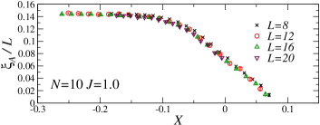
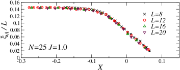
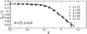
Figure 2: Plot of $R_{A}=\xi_{A}/L$ versus $X=(\kappa-\kappa_{c})L^{1/\nu}$ with $\nu=0.6717$ for: a) $N=1$, $J=1$; b) $N=2$, $J=1$; c) $N=4$, $J=1$; d) $N=10$, $J=1$; e) $N=25$, $J=1$; f) $N=25$, $J=0.4$.

Table 1: Estimates of the critical-point values of the RG-invariant quantities $R_{z}$, $R_{A}$, $U_{z}$ and $U_{A}$, for the different values of $N$. They turn out to be in good agreement, supporting universality.

	$N=1$	$N=2$	$N=4$	$N=10$	$N=25$, $J=1$	$N=25$, $J=0.4$
$R_{z}^{*}$	1.45(5)	1.42(8)	1.35(12)	1.45(10)	1.40(10)	$>1.25$
$R_{A}^{*}$	0.064(4)	0.067(5)	0.075(9)	0.069(6)	0.073(6)	0.071(6)
$U_{z}^{*}$	1.078(10)	1.080(13)	1.09(3)	1.08(2)	1.081(17)	1.12(5)
$U_{A}^{*}$	3.3(1)	3.5(1)	3.6(2)	3.7(2)	3.7(3)	3.2(2)

V.3 The gauge-invariant energy cumulants

MC results for $B_{3}$ are reported in Fig. 3 for $N=1$, $N=2$ (for $J=1$) and $N=25$ (for $J=0.4$). Analogous results are obtained for $N=4,\,10,\,25$ at $J=1$. The observed behaviors are definitely consistent with Eq. (40), when using the $XY$ exponent $\nu_{XY}=0.6717$. Note that, if we appropriately tune the vertical and horizontal scale by adding two nonuniversal constants, the scaling behavior is universal, i.e., the scaling curve is quantitatively the same for all values of $N$ and for the $IXY$ model at $J=\infty$. The scaling curve of the $IXY$ model has been computed in Ref. BPV-24 , by performing an interpolation of MC results for the $IXY$ model. Analogous results are obtained for the higher cumulants. We can therefore conclude that transitions along the MH line for any $N\geq 2$ and along the CH line for $N=1$ have the same $IXY$ universal behavior.

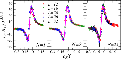
Figure 3: Scaling plot of $B_{3}$ for $N=1$, $N=2$ (for $J=1$) and $N=25$ (for $J=0.4$), from left to right. We plot $\widetilde{\cal B}_{3}=c_{B}B_{3}L^{3-3/\nu}$ versus $\widetilde{X}=c_{X}(\kappa-\kappa_{c})L^{1/\nu}$, fixing $\nu=\nu_{XY}\approx 0.6717$ and the the critical values $\kappa_{c}=0.10745(5),\,0.08931(5),\,0.07996(4)$, respectively. The continuous curve that appears in the three panels is the scaling curve computed in the $IXY$ model BPV-24 with $c_{X}=c_{B}=1$. The nonuniversal constants $c_{X}$ and $c_{B}$ of the LAH models are fixed by matching the curves, obtaining $c_{B}=1.5,1.05,0.95$ and $c_{X}=0.52,0.75,0.9$ for $N=1,2,25$, respectively. Analogous results are obtained for $N=4,\,10,\,25$ along the $J=1$ line.

V.4 Nonlocal charged correlations

We now determine the critical behavior of the charged operator ${\bm{\Gamma}}_{\bm{x}}$ defined in Eq. (29). Charged correlations are expected to have a nontrivial behavior along the MH line. Indeed, in the H phase we have $G_{\Gamma}({\bm{x}},{\bm{y}})\to c\neq 0$ (thus, $G_{z}({\bm{x}},{\bm{y}})\to c\neq 0$ in the Lorenz gauge) in the large $|{\bm{x}}-{\bm{y}}|$ limit, as demonstrated for $N=1$ KK-85 ; KK-86 ; BN-86 ; BN-86-b and numerically confirmed for multicomponent systems BPV-23b .

The numerical results confirm that charged correlations have an $N$-independent critical behavior, which is the same as that occurring in the one-component LAH model along the CH line. In particular, the Lorentz-gauge susceptibility $\chi_{z}$ scales as

$$\chi_{z}\approx L^{2-\eta_{z}}F_{\chi}(X),$$ (43)

with $\eta_{z}$ independent of $N$. The analysis of the scalar correlations in the Lorenz gauge gives $\eta_{z}=-0.74(4)$, $-0.76(2)$, $-0.74(3)$, $-0.75(3)$, $-0.72(4)$ for $N=1,2,4,10,25$ (in all cases $J=1$). We thus end up with the $N$-independent estimate

$$\eta_{z}=-0.74(4).$$ (44)

The plots of the MC data of $\chi_{z}$ shown in Fig. 4 nicely support the scaling behavior (43) with the above estimate of $\eta_{z}$.

To provide additional, and more compelling, evidence that the critical MH transitions belong to the same universality class, irrespective of the value of $N$, we consider the FSS relation $U_{z}\approx F_{U}(R_{z})$ between the Binder parameter and $R_{z}\equiv\xi_{z}/L$. For given boundary conditions and lattice shape, the function $F_{U}$ depends only on the universality class, without requiring the tuning of nonuniversal parameters PV-02 ; BPV-21-ncAH . The scaling curves shown in Fig. 5 are the same for all values of $N$, confirming that the critical behavior of the charged sector is $N$ independent.

It is interesting to observe that these results are also relevant for the $IXY$ model as they characterize the critical behavior of the nonlocal operator $\widetilde{\Gamma}_{\bm{x}}$, that corresponds to the insertion of static charges in the system.

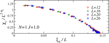
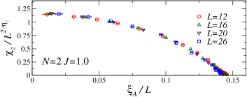
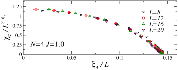
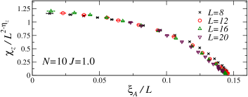
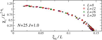
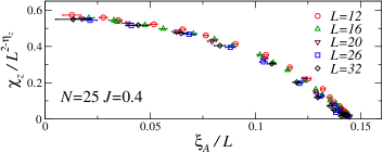
Figure 4: Plot of $\chi_{z}/L^{2-\eta_{z}}$ for $\eta_{z}=-0.74$ versus $R_{A}=\xi_{A}/L$ for: a) $N=1$, $J=1$; b) $N=2$, $J=1$; c) $N=4$, $J=1$; d) $N=10$, $J=1$; e) $N=25$, $J=1$; f) $N=25$, $J=0.4$. The data approach a unique curve, apart from a multiplicative normalization, supporting universality.

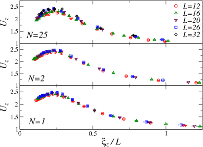
Figure 5: The Binder parameter $U_{z}$ versus the ratio $R_{z}=\xi_{z}/L$ in the Lorenz gauge, for $N=25$ with $J=0.4$ (top), $N=2$ (middle) and $N=1$ (bottom) with $J=1$. They appear to converge to the same universal curve. Analogous results are obtained for $N=4,\,10,\,25$ at $J=1$.

V.5 Local gauge correlations

Gauge and charged correlations show a critical behavior for any $N$. The FSS analysis of the $F_{{\bm{x}},\mu\nu}$ correlations or, equivalently, of the susceptibility $\chi_{A}=V^{-1}\sum_{{\bm{x}}{\bm{y}}}C_{\mu\mu}({\bm{x}},{\bm{y}})$ in the Lorenz gauge BPV-23b , allows us to estimate the gauge-field exponent $\eta_{A}$ ($\chi_{A}\sim L^{2-\eta_{A}}$ at the critical point). In the $IXY$ model we have $\eta_{A}=1$, an exact result that follows from the correspondence between the small-momentum correlation of $F_{{\bm{x}},\mu\nu}$ in the $IXY$ model and the helicity modulus $\Upsilon$ computed in the dual $XY$ model NRR-03 , and from the fact that $\Upsilon$ scales as $L^{-1}$ in the $XY$ model FBJ-73 . If the critical behavior along the MH line (CH line for $N=1$) is the same as in the $IXY$ model, we expect $\eta_{A}=1$ in all cases.

This result is confirmed by the numerical analyses of $\chi_{A}$ for all values of $N$ considered. Note that $\eta_{A}=1$ also holds along the CH line for $N>N^{\star}$, where the transition is controlled by the charged fixed point of the RG flow of the AHFT BPV-23b ; HT-96 ; HS-00 ; KNS-02 ; BFLLW-96 , and, more generally, at any continuous transition controlled by a charged field-theoretical fixed point, as a consequence of the Ward identities ZJ-book .

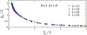
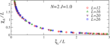
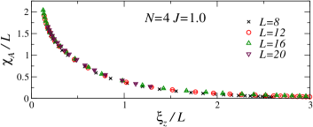
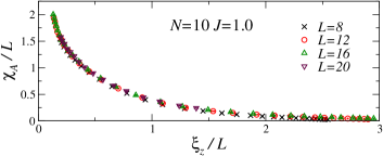
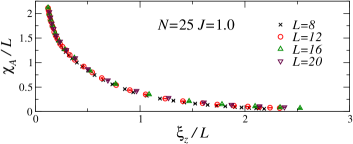
Figure 6: Plot of $\chi_{A}/L^{2-\eta_{A}}=\chi_{A}/L$ ($\eta_{A}=1$) versus $R_{z}=\xi_{z}/L$ for: a) $N=1$, $J=1$; b) $N=2$, $J=1$; c) $N=4$, $J=1$; d) $N=10$, $J=1$; e) $N=25$, $J=1$; f) $N=25$, $J=0.4$. The data approach a unique curve, apart from a multiplicative normalization, supporting universality. For $R_{z}\to 0$ data scale as $1/R_{z}$, to guarantee the correct Coulomb behavior of the susceptibility $\chi_{A}\sim L^{2}$.

VI Conclusions

We have studied the topological phase transitions occurring in the 3D LAH model, in which an $N$-component scalar field is minimally coupled with a noncompact Abelian gauge field, with a global $SU(N)$ symmetry. The phase diagram, see Fig. 1, presents three phases, which differ in the properties of the gauge correlations, in the confinement or deconfinement of the charged excitations, and in the behavior under global $SU(N)$ transformations.

We have shown that multicomponent LAH models can undergo different types of transitions driven by the condensation of charged excitations: CH and MH transitions along the lines that separate the H phase from the C and M phase, respectively. They are controlled by different charged fixed points of the renormalization-group (RG) flow with nonvanishing gauge coupling. Gauge correlations play an active, but different, role at these deconfinement transitions and, therefore, they cannot be described by effective LGW theories. While transitions along the CM and CH lines are related to the spontaneous breaking of the global $SU(N)$ symmetry, the MH line separates two ordered phases, both characterized by the condensation of a gauge-invariant bilinear of the scalar field. The MH transitions are driven by gauge modes that undergo a critical transition without a local gauge-invariant order parameter, as it also occurs for the CH transitions in the one-component LAH model, see Fig. 1.

The numerical results we have presented show that, for any $N\geq 2$ (including the $N\to\infty$ limit), the topological MH transitions belong to the same universality class as the transitions along the CH line for $N=1$. Charged excitations associated with ${\bm{\Gamma}}_{\bm{x}}$, deconfine at the transition. In the Lorenz gauge, ${\bm{\Gamma}}_{\bm{x}}$ is equivalent to the scalar field ${\bm{z}}_{\bm{x}}$ and it is therefore a local operator, allowing us to exploit the standard RG framework. We estimate the RG dimension of ${\bm{\Gamma}}_{\bm{x}}$, obtaining $y_{\Gamma}=(d-2+\eta_{z})/2\approx 0.13(2)$. We observe that excitations with RG dimensions $y_{\Gamma}$ also exist in the $IXY$ model, i.e., in the absence of explicit scalar fields, and are associated with the operator $\widetilde{\Gamma}_{\bm{x}}$ defined in Eq. (34). We finally note that charged excitations are also relevant along the CH line BPV-23b . The ${\bm{\Gamma}}_{\bm{x}}$ operator has here a different $N$-dependent RG dimension $y_{\Gamma}$: $y_{\Gamma}=0.4655(5)$ for $N=25$ BPV-23b and $y_{\Gamma}\approx 1/2-10/(\pi^{2}N)$ for large $N$ HLM-74 ; KS-08 .

We have also discussed the critical behavior of gauge local correlations, showing that the associated susceptibility exponent $\eta_{A}$ satisfies $\eta_{A}=1$, as in the $IXY$ model. For the latter model $\eta_{A}=1$ is an exact result that can be proved using duality.

Note that, although the $IXY$ model is dual to the $XY$ model, the critical behavior of the charged scalar correlations along the $N=1$ CH line is not related to that of the scalar correlations in the $XY$ model obtained for $\kappa\to\infty$, see Fig. 1. Obviously, the Lorenz-gauge correlations of the field ${\bm{z}}_{\bm{x}}$ along the CH line converge to the scalar correlations of the $XY$ model for $\kappa\to\infty$ at fixed system size $L$. However, since the $\kappa\to\infty$ and the $L\to\infty$ limits do not commute, this result does not imply that their asymptotic infinite-volume behavior is the same. Indeed, charged scalar correlations are characterized by the critical exponent $\eta_{z}\approx-0.7$ along the CH line at finite $\kappa$, definitely differing from the value $\eta_{z}\approx 0.038$ at the $\kappa=\infty$ $XY$ transition PV-02 . This is consistent with the RG field-theory result that predicts the $XY$ RG fixed point to be unstable with respect to gauge fluctuations BPV-21-ncAH .

Although the CH and MH transitions both separate a phase with confined charges from a deconfined Higgs phase, their critical behavior shows notable differences, since the transitions are associated with different charged RG fixed points. Indeed, the critical MH transitions are effectively controlled by the charged $IXY$ fixed point, while the continuous CH transitions, which occur for $N>N^{\star}\approx 7$ IZMHS-19 ; BPV-21-ncAH ; BPV-22 ; SZJSM-23 , are controlled by the different, $N$-dependent, charged fixed point that is obtained in the AHFT. Estimates of the corresponding $N$-dependent critical exponents are reported in Ref. BPV-21-ncAH ; BPV-23b ; for instance, $\nu=0.802(8)$ for $N=25$, and $\nu\approx 1-48/(\pi^{2}N)$ for large $N$ HLM-74 ; MZ-03 . Therefore, LAH models with $N>N^{\star}$ show two distinct charged critical behaviors along the MH and CH transition lines. Note that, if the MH and CH transitions remain continuous up to their intersection point (they could turn into first-order transitions before it), a nontrivial multicritical behavior can occur PV-02 , calling for further investigations. We finally remark that the $N$-independent MH critical behavior does not have a counterpart in the RG flow of the AHFT, as determined using the perturbative $\epsilon=4-d$ expansion HLM-74 ; IZMHS-19 , or in the standard large-$N$ approach MZ-03 .

It would be interesting to add fermionic fields to the LAH model, minimally coupled to the gauge field. Also in this case one expects Higgs phases bounded by topological transitions. In particular, for large $J$ one still expects a transition line where gauge fields behave as in the $IXY$ model. While massive fermions should not change the critical behaviors (they can be effectively integrated out), massless fermions may lead to different topological universality classes, which may be of interest for condensed-matter systems. At these transitions the charged gauge-invariant fermionic excitations Dirac:1955uv may be studied as the scalar ones. Topological charged transitions driven by gauge fields can also be present in 3D non-Abelian gauge theories with scalar fields in diverse representations, see, e.g., Refs. Sachdev-19 ; SSST-19 ; BPV-19 ; SPSS-20 ; BFPV-21 . However, in this case the identification of the relevant gauge-invariant matter excitations is more complex. In particular, the nonlinearity of the gauge conditions Faddeev:1967fc ; Gribov:1977wm ; Singer:1978dk does not allow us to extend to the non-Abelian case the simple gauge-fixing approach exploited in this work. These issues call for further investigation.

References

- (1) P. W. Anderson, Basic Notions of Condensed Matter Physics, (The Benjamin/Cummings Publishing Company, Menlo Park, California, 1984).
- (2) X.-G. Wen, Quantum field theory of many-body systems: from the origin of sound to an origin of light and electrons, (Oxford University Press, 2004).
- (3) B. I. Halperin, T. C. Lubensky, and S. K. Ma, First-Order Phase Transitions in Superconductors and Smectic-A Liquid Crystals, Phys. Rev. Lett. 32, 292 (1974).
- (4) I. Herbut, A Modern Approach to Critical Phenomena (Cambridge University Press, 2007).
- (5) N. Read and S. Sachdev, Spin-Peierls, valence-bond solid, and Néel ground states of low-dimensional quantum antiferromagnets, Phys. Rev. B 42, 4568 (1990).
- (6) S. Takashima, I. Ichinose, and T. Matsui, CP1+U(1) lattice gauge theory in three dimensions: Phase structure, spins, gauge bosons, and instantons, Phys. Rev. B 72, 075112 (2005).
- (7) S. Takashima, I. Ichinose, and T. Matsui, Deconfinement of spinons on critical points: Multiflavor CP1+U(1) lattice gauge theory in three dimension, Phys. Rev. B 73, 075119 (2006).
- (8) R. K. Kaul, Quantum phase transitions in bilayer antiferromagnets, Phys. Rev. B 85, 180411(R) (2012).
- (9) R. K. Kaul and A. W. Sandvik, Lattice Model for the Néel to Valence-Bond Solid Quantum Phase Transition at Large , Phys. Rev. Lett. 108, 137201 (2012).
- (10) M. S. Block, R. G. Melko, and R. K. Kaul, Fate of CPN-1 fixed point with monopoles, Phys. Rev. Lett. 111, 137202 (2013).
- (11) A. Nahum, J. T. Chalker, P. Serna, M. Ortuǹo, and A. M. Somoza, Deconfined Quantum Criticality, Scaling Violations, and Classical Loop Models, Phys. Rev. X 5, 041048 (2015).
- (12) C. Wang, A. Nahum, M. A. Metliski, C. Xu, and T. Senthil, Deconfined Quantum Critical Points: Symmetries and Dualities, Phys. Rev. X 7, 031051 (2017).
- (13) S. Sachdev, Topological order, emergent gauge fields, and Fermi surface reconstruction, Rep. Prog. Phys. 82, 014001 (2019).
- (14) A. W. Sandvik, Evidence for Deconfined Quantum Criticality in a Two-Dimensional Heisenberg Model with Four-Spin Interactions, Phys. Rev. Lett. 98, 227202 (2007).
- (15) R. G. Melko and R. K. Kaul, Scaling in the Fan of an Unconventional Quantum Critical Point, Phys. Rev. Lett. 100, 017203 (2008).
- (16) F. J. Jiang, M. Nyfeler, S. Chandrasekharan, and U. J. Wiese, From an Antiferromagnet to a Valence Bond Solid: Evidence for a First-Order Phase Transition, J. Stat. Mech. (2008) P02009.
- (17) A. W. Sandvik, Continuous Quantum Phase Transition between an Antiferromagnet and a Valence-Bond Solid in Two Dimensions: Evidence for Logarithmic Corrections to Scaling, Phys. Rev. Lett. 104, 177201 (2010).
- (18) K. Harada, T. Suzuki, T. Okubo, H. Matsuo, J. Lou, H. Watanabe, S. Todo, and N. Kawashima, Possibility of Deconfined Criticality in Heisenberg Models at Small , Phys. Rev. B 88, 220408 (2013).
- (19) K. Chen, Y. Huang, Y. Deng, A. B. Kuklov, N. V. Prokof’ev, and B.V. Svistunov, Deconfined Criticality Flow in the Heisenberg Model with Ring-Exchange Interactions, Phys. Rev. Lett. 110, 185701 (2013).
- (20) S. Pujari, K. Damle, and F. Alet, Nèel-State to Valence-Bond-Solid Transition on the Honeycomb Lattice: Evidence for Deconfined Criticality, Phys. Rev. Lett. 111, 087203 (2013).
- (21) H. Shao, W. Guo, and A. W. Sandvik, Quantum criticality with two length scales, Science 352, 213 (2016).
- (22) T. Senthil, L. Balents, S. Sachdev, A. Vishwanath, and M. P. A. Fisher, Quantum Criticality beyond the Landau-Ginzburg-Wilson Paradigm, Phys. Rev. B 70, 144407 (2004).
- (23) E. Fradkin and S. Shenker, Phase diagrams of lattice gauge theories with Higgs fields, Phys. Rev. D 19, 3682 (1979).
- (24) C. Dasgupta and B. I. Halperin, Phase Transitions in a Lattice Model of Superconductivity, Phys. Rev. Lett 47, 1556 (1981).
- (25) J. Frohlich, G. Morchio, and F. Strocchi, Higgs phenomenon without symmetry breaking order parameter, Nucl. Phys. B190, 553 (1981).
- (26) P. Di Vecchia, A. Holtkamp, R. Musto, F. Nicodemi, and R. Pettorino, Lattice CPN-1 models and their large- behaviour, Nucl. Phys. B 190, 719 (1981).
- (27) D. J. E. Callaway and L. J. Carson, Abelian Higgs model: A Monte Carlo study, Phys. Rev. D 25, 531 (1982).
- (28) J. Bricmont and J. Frohlich, An order parameter distinguishing between different phases of lattice gauge theories with matter fields, Phys. Lett. 122, 73 (1983).
- (29) K. Fredenhagen and M. Marcu, Charged states in gauge theories, Commun. Math. Phys. 92, 81 (1983).
- (30) T. Kennedy and C. King, Symmetry Breaking in the Lattice Abelian Higgs Model, Phys. Rev. Lett. 55, 776 (1985).
- (31) T. Kennedy and C. King, Spontaneous Symmetry Breakdown in the Abelian Higgs Model, Commun. Math. Phys. 104, 327 (1986).
- (32) C. Borgs and F. Nill, Symmetry Breaking in Landau Gauge A comment to a paper by T. Kennedy and C. King, Commun. Math. Phys. 104, 349 (1986).
- (33) C. Borgs and F. Nill, No Higgs mechanism in scalar lattice QED with strong electromagnetic coupling, Phys. Lett. B 171, 289 (1986).
- (34) C. Borgs and F. Nill, The Phase Diagram of the Abelian Lattice Higgs Model. A Review of Rigorous Results, J. Stat. Phys. 47, 877 (1987).
- (35) G. Murthy and S. Sachdev, Actions of hedgehogs instantons in the disordered phase of 2+1 dimensional CPN-1 model, Nucl. Phys. B 344, 557 (1990).
- (36) M. Kiometzis, H. Kleinert, and A. M. J. Schakel, Critical Exponents of the Superconducting Phase Transition, Phys. Rev. Lett. 73, 1975 (1994).
- (37) B. Bergerhoff, F. Freire, D.F. Litim, S. Lola, and C. Wetterich, Phase diagram of superconductors from nonperturbative flow equations, Phys. Rev. B 53, 5734 (1996).
- (38) F. Herbut and Z. Tesanovic, Critical Fluctuations in Superconductors and the Magnetic Field Penetration Depth, Phys. Rev. Lett. 76, 4588 (1996).
- (39) R. Folk and Y. Holovatch, On the critical fluctuations in superconductors, J. Phys. A 29, 3409 (1996).
- (40) V. Yu. Irkhin, A. A. Katanin, and M. I. Katsnelson, expansion for critical exponents of magnetic phase transitions in the model for , Phys. Rev. B 54, 11953 (1996).
- (41) K. Kajantie, M. Karjalainen, M. Laine, and J. Peisa, Masses and phase structure in the Ginzburg-Landau model, Phys. Rev. B 57, 3011 (1998).
- (42) P. Olsson and S. Teitel, Critical Behavior of the Meissner Transition in the Lattice London Superconductor, Phys. Rev. Lett. 80, 1964 (1998).
- (43) C. de Calan and F.S. Nogueira, Scaling critical behavior of superconductors at zero magnetic field, Phys. Rev. B 60, 4255 (1999)
- (44) J. Hove and A. Sudbo, Anomalous Scaling Dimensions and Stable Charged Fixed Point of Type-II Superconductors, Phys. Rev. Lett. 84, 3426 (2000).
- (45) H. Kleinert, F. S. Nogueira, and A. Sudbø, Deconfinement Transition in Three-Dimensional Compact U(1) Gauge Theories Coupled to Matter Fields, Phys. Rev. Lett. 88, 232001 (2002).
- (46) S. Mo, J. Hove, and A. Sudbø, Order of the metal-to-superconductor transition, Phys. Rev. B 65, 104501 (2002).
- (47) A. Sudbø, E. Smørgrav, J. Smiseth, F. S. Nogueira, and J. Hove, Criticality in the (2+1)-Dimensional Compact Higgs Model and Fractionalized Insulators, Phys. Rev. Lett. 89, 226403 (2002).
- (48) J. Smiseth, E. Smørgrav, F. S. Nogueira, J. Hove, and A. Sudbø, Phase Structure of Compact Lattice Gauge Theories and the Transition from Mott Insulator to Fractionalized Insulator, Phys. Rev. B 67, 205104 (2003).
- (49) M. Moshe and J. Zinn-Justin, Quantum field theory in the large limit: A review, Phys. Rep. 385, 69 (2003).
- (50) T. Neuhaus, A. Rajantie, and K. Rummukainen, Numerical study of duality and universality in a frozen superconductor, Phys. Rev. B 67, 014525 (2003).
- (51) O. I. Motrunich and A. Vishwanath, Emergent photons and transitions in the O(3) -model with hedgehog suppression, Phys. Rev. B 70, 075104 (2004).
- (52) F. S. Nogueira, J. Smiseth, E. Smørgrav, and A. Sudbø, Compact U(1) gauge theories in dimensions and the physics of low dimensional insulating materials, Eur. Phys. J. C 33, 885 (2004).
- (53) J. Smiseth, E. Smorgrav, and A. Sudbø, Critical properties of the -color London model, Phys. Rev. Lett. 93, 077002 (2004).
- (54) S. Wenzel, E. Bittner, W. Janke, A. M. J. Schakel, and A. Schiller, Kertesz Line in the Three-Dimensional Compact U(1) Lattice Higgs Model, Phys. Rev. Lett. 95, 051601 (2005).
- (55) M. N. Chernodub, R. Feldmann, E.-M. Ilgenfritz, and A. Schiller, The compact Abelian Higgs model in the London limit: vortex-monopole chains and the photon propagator, Phys. Rev. D 71, 074502 (2005).
- (56) M. B. Hastings and X.-G. Wen, Quasi-adiabatic Continuation of Quantum States: The Stability of Topological Ground State Degeneracy and Emergent Gauge Invariance, Phys. Rev. B 72, 045141 (2005)
- (57) M. N. Chernodub, E.-M. Ilgenfritz, and A. Schiller, Phase structure of an Abelian two-Higgs model and high temperature superconductors, Phys. Rev. B 73, 100506 (2006).
- (58) A. B. Kuklov, N. V. Prokof’ev, B. V. Svistunov, and M. Troyer, Deconfined criticality, runaway flow in the two-component scalar electrodynamics and weak first-order superfluid-solid transitions, Ann. Phys. 321, 1602 (2006).
- (59) S. Wenzel, E. Bittner, W. Janke, and A. M. J. Schakel, Percolation of Vortices in the 3D Abelian Lattice Higgs Model, Nucl. Phys. B 793, 344 (2008).
- (60) O. I. Motrunich and A. Vishwanath, Comparative study of Higgs transition in one-component and two-component lattice superconductor models, arXiv:0805.1494 [cond-mat.stat-mech].
- (61) A. B. Kuklov, M. Matsumoto, N. V. Prokof’ev, B. V. Svistunov, and M. Troyer, Deconfined Criticality: Generic First-Order Transition in the SU(2) Symmetry Case, Phys. Rev. Lett. 101, 050405 (2008).
- (62) D. Charrier, F. Alet, and P. Pujol, Gauge Theory Picture of an Ordering Transition in a Dimer Model, Phys. Rev. Lett. 101, 167205 (2008).
- (63) R. K. Kaul and S. Sachdev, Quantum criticality of U(1) gauge theories with fermionic and bosonic matter in two spatial dimensions, Phys. Rev. B 77, 155105 (2008).
- (64) T. Ono, S. Doi, Y. Hori, I. Ichinose, and T. Matsui, Phase Structure and Critical Behavior of Multi-Higgs U(1) Lattice Gauge Theory in Three Dimensions, Ann. Phys. (N.Y.) 324, 2453 (2009).
- (65) J. Lou, A. W. Sandvik, and N. Kawashima, Antiferromagnetic to valence-bond-solid transitions in two-dimensional SU(N) Heisenberg models with multispin interactions, Phys. Rev. B 80, 180414 (2009).
- (66) G. Chen, J. Gukelberger, S. Trebst, F. Alet, and L. Balents, Coulomb gas transitions in three-dimensional classical dimer models, Phys. Rev. B 80, 045112 (2009).
- (67) D. Charrier and F. Alet, Phase diagram of an extended classical dimer model, Phys. Rev. B 82, 014429 (2010).
- (68) A. Banerjee, K. Damle, and F. Alet, Impurity spin texture at a deconfined quantum critical point, Phys. Rev. B 82, 155139 (2010).
- (69) E. V. Herland, T. A. Bojesen, E. Babaev, and A. Sudbø, Phase structure and phase transitions in a three-dimensional SU(2) superconductor, Phys. Rev. B 87, 134503 (2013).
- (70) L. Bartosch, Corrections to scaling in the critical theory of deconfined criticality, Phys. Rev. B 88, 195140 (2013).
- (71) T. A. Bojesen and A. Sudbø, Berry phases, current lattices, and suppression of phase transitions in a lattice gauge theory of quantum antiferromagnets, Phys. Rev. B 88, 094412 (2013).
- (72) A. Nahum, P. Serna, J. T. Chalker, M. Ortuǹo, and A. M. Somoza, Emergent SO(5) Symmetry at the Néel to Valence-Bond-Solid Transition, Phys. Rev. Lett. 115, 267203 (2015).
- (73) G. J. Sreejith and S. Powell, Scaling dimensions of higher-charge monopoles at deconfined critical points, Phys. Rev. B 92, 184413 (2015).
- (74) G. Fejos and T. Hatsuda, Renormalization group flows of the -component Abelian Higgs model, Phys. Rev. D 96, 056018 (2017).
- (75) B. Ihrig, N. Zerf, P. Marquard, I. F. Herbut, and M. M. Scherer, Abelian Higgs model at four loops, fixed-point collision and deconfined criticality, Phys. Rev. B 100, 134507 (2019).
- (76) P. Serna and A. Nahum, Emergence and spontaneous breaking of approximate O(4) symmetry at a weakly first-order deconfined phase transition, Phys. Rev. B 99, 195110 (2019).
- (77) A. Pelissetto and E. Vicari, Three-dimensional ferromagnetic CPN-1 models, Phys. Rev. E 100, 022122 (2019).
- (78) A. Pelissetto and E. Vicari, Multicomponent compact Abelian-Higgs lattice models, Phys. Rev. E 100, 042134 (2019).
- (79) A. W. Sandvik and B. Zhao, Consistent scaling exponents at the deconfined quantum-critical point, Chin. Phys. Lett. 37, 057502 (2020).
- (80) A. Pelissetto and E. Vicari, Three-dimensional monopole-free CPN-1 models, Phys. Rev. E 101, 062136 (2020).
- (81) A. Pelissetto and E. Vicari, Large- behavior of three-dimensional lattice CPN-1 models, J. Stat. Mech.: Th. Expt. 033209 (2020).
- (82) C. Bonati, A. Pelissetto, and E. Vicari, Higher-charge three-dimensional compact lattice Abelian-Higgs models, Phys. Rev. E 102, 062151 (2020).
- (83) C. Bonati, A. Pelissetto, and E. Vicari, Lattice Abelian-Higgs model with noncompact gauge fields, Phys. Rev. B 103, 085104 (2021).
- (84) C. Bonati, A. Pelissetto and E. Vicari, Breaking of Gauge Symmetry in Lattice Gauge Theories, Phys. Rev. Lett. 127, 091601 (2021)
- (85) C. Bonati, A. Pelissetto, and E. Vicari, Lattice gauge theories in the presence of a linear gauge-symmetry breaking, Phys. Rev. E 104, 014140 (2021).
- (86) D. Weston and E. Babaev, Composite order in theories coupled to an Abelian gauge field, Phys. Rev. B 104, 075116 (2021).
- (87) C. Bonati, A. Pelissetto, and E. Vicari, Three-dimensional monopole-free CPN-1 models: Behavior in the presence of a quartic potential, J. Stat. Mech. (2022) 063206.
- (88) C. Bonati, A. Pelissetto, and E. Vicari, Critical behaviors of lattice U(1) gauge models and three-dimensional Abelian-Higgs gauge field theory, Phys. Rev. B 105, 085112 (2022).
- (89) C. Bonati, A. Pelissetto, and E. Vicari, Coulomb-Higgs phase transition of three-dimensional lattice Abelian Higgs gauge models with noncompact gauge variables and gauge fixing, Phys. Rev. E 108, 044125 (2023).
- (90) M. Song, J. Zhao, L. Janssen, M. M. Scherer, and Z. Y. Meng, Deconfined quantum criticality lost, arXiv:2307.02547.
- (91) C. Bonati, A. Pelissetto, and E. Vicari, Deconfinement transitions in three-dimensional compact lattice Abelian Higgs models with multiple-charge scalar fields, in preparation.
- (92) J. Zinn-Justin, Quantum Field Theory and Critical Phenomena (Clarendon Press, 2002)
- (93) A. Pelissetto and E. Vicari, Critical Phenomena and Renormalization Group Theory, Phys. Rep. 368, 549 (2002).
- (94) S. Sachdev, Quantum Phase Transitions, (Cambridge University, Cambridge, England, 1999).
- (95) P. A. M. Dirac, Gauge invariant formulation of quantum electrodynamics, Can. J. Phys. 33, 650 (1955).
- (96) A. S. Kronfeld and U. J. Wiese, SU(N) gauge theories with C periodic boundary conditions. 1. Topological structure, Nucl. Phys. B 357, 521 (1991).
- (97) B. Lucini, A. Patella, A. Ramos, and N. Tantalo, Charged hadrons in local finite-volume QED+QCD with C∗ boundary conditions, JHEP 02, 076 (2016).
- (98) C. Bonati, A. Pelissetto, and E. Vicari, Gauge fixing and gauge correlations in noncompact Abelian gauge models, Phys. Rev. D 108, 014517 (2023).
- (99) M. Hasenbusch, Monte Carlo study of an improved clock model in three dimensions, Phys. Rev. B 100, 224517 (2019).
- (100) M. Campostrini, M. Hasenbusch, A. Pelissetto, and E. Vicari, Theoretical estimates of the critical exponents of the superfluid transition in 4He by lattice methods, Phys. Rev. B 74, 144506 (2006).
- (101) Y. Deng, H. W. J. Blöte, and M. P. Nightingale, Surface and bulk transitions in three-dimensional models, Phys. Rev. E 72, 016128 (2005).
- (102) M. Hasenbusch, Three-dimensional O(N)-invariant models at criticality for , Phys. Rev. B 105, 054428 (2022).
- (103) M. Campostrini, A. Pelissetto, P. Rossi, E. Vicari, Four-point renormalized coupling in O() models, Nucl. Phys. B 459, 207 (1996).
- (104) C. Bonati, A. Pelissetto, and E. Vicari, Multicritical point of the three-dimensional Z2 gauge Higgs model, Phys. Rev. B 105, 165138 (2022).
- (105) S. M. Chester, W. Landry, J. Liu, D. Poland, D. Simmons-Duffin, N. Su, and A. Vichi, Carving out OPE space and precise O(2) model critical exponents, J. High Energy Phys. 06, 142 (2020).
- (106) R. Guida and J. Zinn-Justin, Critical exponents of the -vector model, J. Phys. A 31, 8103 (1998).
- (107) M. V. Kompaniets and E. Panzer, Minimally subtracted six-loop renormalization of -symmetric theory and critical exponents, Phys. Rev. D 96, 036016 (2017).
- (108) K. G. Wilson, The renormalization group and critical phenomena, Rev. Mod. Phys 55, 583 (1983).
- (109) M. E. Fisher, The renormalization group in the theory of critical behavior, Rev. Mod. Phys. 47, 543 (1975).
- (110) F. J. Wegner, The critical state, general aspects, in Phase transitions and critical phenomena, vol. 6, p. 7, edited by C. Domb and M. S. Green (Academic Press, London, 1976).
- (111) V. Privman (Ed.), Finite size scaling and numerical simulation of statistical systems (World Scientific, Singapore, 1990).
- (112) M. E. Fisher, M. N. Barber, and D. Jasnow, Helicity modulus, superfluidity, and scaling in isotropic systems, Phys. Rev. A 8, 1111 (1973).
- (113) S. Sachdev, H. D. Scammell, M. S. Scheurer, and G. Tarnopolsky, Gauge theory for the cuprates near optimal doping, Phys. Rev. B 99, 054516 (2019).
- (114) C. Bonati, A. Pelissetto, and E. Vicari, Phase Diagram, Symmetry Breaking, and Critical Behavior of Three-Dimensional Lattice Multiflavor Scalar Chromodynamics, Phys. Rev. Lett. 123, 232002 (2019); Three-dimensional lattice multiflavor scalar chromodynamics: Interplay between global and gauge symmetries, Phys. Rev. D 101, 034505 (2020); Phase diagram and Higgs phases of 3D lattice SU() gauge theories with multiparameter scalar potentials, Phys. Rev. E 104, 064111 (2021).
- (115) H. D. Scammell, K. Patekar, M. S. Scheurer, and S. Sachdev, Phases of SU(2) gauge theory with multiple adjoint Higgs fields in 21 dimensions, Phys. Rev. B 101, 205124 (2020).
- (116) C. Bonati, A. Franchi, A. Pelissetto, and E. Vicari, Three-dimensional lattice SU() gauge theories with multiflavor scalar fields in the adjoint representation, Phys. Rev B 114, 115166 (2021).
- (117) L. D. Faddeev and V. N. Popov, Feynman Diagrams for the Yang-Mills Field, Phys. Lett. B 25, 29 (1967).
- (118) V. N. Gribov, Quantization of Nonabelian Gauge Theories, Nucl. Phys. B 139, 1 (1978).
- (119) I. M. Singer, Some Remarks on the Gribov Ambiguity, Commun. Math. Phys. 60, 7 (1978).