Visual Geo-localization with Self-supervised Representation Learning

Abstract

Visual Geo-localization (VG) has emerged as a significant research area, aiming to identify geolocation based on visual features. Most VG approaches use learnable feature extractors for representation learning. Recently, Self-Supervised Learning (SSL) methods have also demonstrated comparable performance to supervised methods by using numerous unlabeled images for representation learning. In this work, we present a novel unified VG-SSL framework with the goal to enhance performance and training efficiency on a large VG dataset by SSL methods. Our work incorporates multiple SSL methods tailored for VG: SimCLR, MoCov2, BYOL, SimSiam, Barlow Twins, and VICReg. We systematically analyze the performance of different training strategies and study the optimal parameter settings for the adaptation of SSL methods for the VG task. The results demonstrate that our method, without the significant computation and memory usage associated with Hard Negative Mining (HNM), can match or even surpass the VG performance of the baseline that employs HNM. The code is available at https://github.com/arplaboratory/VG_SSL.

1 Introduction

Visual Geo-localization (VG), also known as Visual Place Recognition, is a computer vision [9, 8, 2, 4] and robotics [10, 20, 14, 46] active research area that has gained tremendous popularity and interest in these past years. It focuses on a task aiming to identify geographical locations based on visual features. Most VG approaches adopt the image retrieval (IR) paradigm. It involves building a database by using a visual feature extractor to generate robust compact representation (e.g., embeddings or histogram of orientation [32]) from a large set of geo-referenced images (i.e., with longitude and latitude data). Recent VG methods mostly exploit the expressive power of deep neural networks [31] to learn useful representations for this task. These approaches generally project images into an embedding space and employ these embeddings as data representations for the VG task. Given the representation of the query image, the approaches can match it to the most similar ones in the database and retrieve geo-referenced information. For accurate matching, the feature extractor should output recognizable and robust representations. Therefore, the learning mechanism of this feature extractor aligns with representation learning, a more general topic that focuses on generating robust and informative data representation with or without being tied to specific downstream tasks. It has become prevalent in computer vision, natural language processing [7], and robotics [39].

Over the last few years, Self-Supervised Learning (SSL) methods are emerging as popular solutions for representation learning in computer vision. These methods rely on pre-training feature extractors on pretext tasks [35] with vast amounts of unlabeled data to learn visual representation. Once pre-training, these models can be fine-tuned by freezing the pre-trained feature extractor and training additional downstream heads for specific tasks (e.g., Multi-Layer Perceptron (MLP) for classification). With a pre-trained feature extractor, these methods can achieve on-par performance with much less labeled data. A common pretext task in self-supervised learning is contrastive learning [11, 25, 12]. This approach aims to minimize the embedding distance between augmented image views of the same scene (i.e., positive samples) and maximize the embedding distance between views of different scenes (i.e., negative samples). Several VG methods [4, 2, 9, 37] adopt contrastive learning strategies (e.g., triplet loss [27], or multi-similarity loss [43]) to obtain a compact representation for VG.

To achieve reliable VG performance, multiple VG methods [1, 9] based on contrastive learning employ Hard Negative Mining (HNM). However, HNM includes caching and ranking all or a subset of negative samples in the database for each sampled query image, leading to significant computation and memory usage, especially in case large databases are employed. In this work, we focus on incorporating SSL methods into VG tasks with the goal of eliminating the need for HNM while concurrently obtaining comparable performances. Specifically, we instantiate our strategy on six state-of-the-art SSL methods: SimCLR [11], MoCov2 [12], BYOL [22], SimSiam [13], Barlow Twins [48] and VicReg [6] and investigate the optimal settings for incorporating these methods for the VG task. By leveraging these pair-wise SSL methods and only selecting positive samples, our framework can get rid of HNM in model training.

The main contributions of our work are as follows: 1) We present a general VG-SSL framework to learn representations for Visual Geo-localization (VG) that unifies and integrates various Self-Supervised-Learning (SSL) methods; 2) we show reduced computation, memory usage at the training stage, and comparable or superior performance with respect to methods utilizing HNM across five public VG datasets; 3) we experimentally study the impact of major parameters in VG-SSL to identify optimal settings in the adaptation of different SSL methods, and to our best knowledge, this is the first work to establish a standardized framework incorporating multiple self-supervised representation learning methods for VG, as well as systematically analyze VG performance of different training strategies.

2 Related Works

Representation Learning for VG. VG methods require extracting appropriate representation from images to differentiate between distinct locations. Traditional VG methods [16, 23, 34, 15] rely on handcrafted templates to extract representations, which are less robust to noise and appearance changes (e.g., illumination change). On the other hand, recent deep learning-based VG approaches [4, 2, 8, 49, 3, 47] achieve state-of-the-art performance by utilizing deep neural networks [31] to learn optimal representations. The architecture incorporates a deep neural network for local feature extraction and a trainable feature aggregation module for generating robust, compact global representations. Feature aggregation techniques such as Maximum Activations of Convolutions (MAC) [38], Generalized Mean (GeM) [37] pooling, NetVLAD [4] (the differentiable version of VLAD [28]), and their various extensions [24, 29, 40] have gained widespread adoption for VG. Typically, VG methods employ contrastive learning to distinguish between positive and negative samples for a query image. A notable recent work [9] benchmarks multiple VG methods for contrastive learning using triplet loss. However, these methods have a significant limitation in the form of considerable time and memory requirements using Hard Negative Mining (HNM) to build triplets. This process involves caching and sorting embeddings for large-scale datasets. Our approach, inspired by self-supervised representation learning, eliminates the need for exhaustive HNM by employing SSL training strategies. It only requires selecting positive samples, enhancing the overall efficiency and effectiveness of VG tasks.

Self-supervised Representation Learning. Self-supervised learning (SSL) has undergone significant progress. In computer vision, some recent advancements achieve similar, or even better performance than supervised methods in downstream tasks by learning the recognizable and invariant visual representation from a large amount of unlabeled image data. The primary challenge in SSL lies in preventing model collapse causing the model to ignore the input and always outputs the same embeddings. We choose several proven methods among different categories: Contrastive Learning [11, 25, 12], Self-distillation Learning [22, 13], and Information Maximization [48, 6]. The features of relevant SSL methods are summarized in Table 1.

Contrastive Learning methods, including SimCLR [11] and MoCov2 [12], optimize to align embeddings of two augmented views of an image and reduce the similarity between the embedding and those from other non-related images. SimCLR [11] uses large batch size for better training and introduces a projector consisting of shallow layers of MLP to reproject the embeddings to projected space. This mitigates the undesired invariance produced by augmentations. MoCo [25] and its variant MoCov2 [12] introduce InfoNCE loss from [36] for visual tasks and a momentum encoder as an alternative for generating key embeddings for a memory dictionary, avoiding the need for large batch sizes.

Self-distillation Learning methods, including BYOL [22] and SimSiam [13], demonstrate the feasibility of preventing collapse by using a teacher-student training framework. They use a predictor to predict the teacher embedding from the student embedding so that the model will attempt to learn the common representation between the student and teacher model inputs. BYOL [22] uses the momentum target (teacher) encoder and an embedding prediction loss, that is cosine distance between predicted and actual teacher embeddings. The target encoder stops the gradients back-propagated from the loss function. SimSiam [13] empirically proves that stop-gradient operation and batch normalization in the projector and predictor play an essential role in avoiding collapse.

Information maximization methods, including Barlow Twins [48] and VICReg [6], aim to decorrelate embeddings of different images to maximize the information contained within the embeddings. Barlow Twins (BT) [48] builds a cross-correlation matrix of embeddings and suppresses the off-diagonal elements to achieve decorrelation. VICReg [6] explicitly uses Variance-Invariance-Covariance (VIC) Regularization loss to maintain the variance of embedding elements above a margin and reduce the covariance between embedding elements to zero for decorrelation. Both methods report similar performance to previous works using smaller batch sizes but require a large dimensionality of projector embedding.

In pursuit of the shared objective of VG and SSL methods to learn invariant and recognizable representations, previous works explore the idea of incorporating SSL into the field of VG. A recent work [44] reviews the SSL methods in the context of classification tasks for remote sensing, adhering to the pretrain-finetune workflow. The authors in [5] employ the MoCov2 [12] framework with a memory dictionary and use the prediction of the geographical information (latitude, longitude, and country) as a pretext task for geography-aware SSL. Conversely, [1] improves hard negative mining in VG using a memory bank like MoCo [25]. Finally, [21] finds the best regions of query images in a self-supervised manner to improve the VG performances. Additionally, [10] proposes an SSL framework to discover spatial neighborhoods for auto-labeling. In contrast to these studies, our work delves into the direct application of SSL training methods for downstream VG training, following the image retrieval paradigm. We also provide a thorough performance comparison with multiple SSL methods in VG tasks.

Table 1: Relevant SSL training methods compared in this work. ME: Momentum target encoder. SG: Stop gradient for target encoder. PR: Predictor for the output of target encoder. BN: Batch normalization in the projector or predictor. LP: Large dimensionality of embeddings.

Categories	Methods	ME	SG	PR	BN	LP	Loss Function
Contrastive Learning	SimCLR [11]						InfoNCE Loss
	MoCov2 [12]	$\checkmark$					InfoNCE Loss
Self-distillation Learning	BYOL [22]	$\checkmark$	$\checkmark$	$\checkmark$	$\checkmark$		Embedding Prediction Loss
	SimSiam [13]		$\checkmark$	$\checkmark$	$\checkmark$		Embedding Prediction Loss
Information Maximization	Barlow Twins [48]				$\checkmark$	$\checkmark$	Cross-correlation Loss
	VICReg [6]				$\checkmark$	$\checkmark$	VIC Regularization Loss

3 Methodology

As depicted in Fig. 1, compared to the VG pipeline with triplet loss [9], our VG-SSL framework modifies the data pipeline with a novel sampling method (detailed in Section 3.2) to accommodate pair-wise SSL training. Additionally, we introduce a projection head, inspired by [11], which follows the feature extractor $F$. These adaptations enable the deployment of SSL training strategies on the output projected embeddings $q,k^{p},k^{n}$. This novel training approach eliminates the hard requirement of HNM, thereby releasing substantial resources previously allocated for HNM in large datasets.

We denote $D$ as the dimension of embeddings, $N$ as the batch size, $L$ as the number of layers in the projection head, and $q$ as the embeddings of query images ($I_{q}$), $k^{p}$ and $k^{n}$ the embeddings of positive ($I_{k^{p}}$) and negative images ($I_{k^{n}}$) related to $q$, respectively. The terms $q_{b}=[q_{b,1},q_{b,2},...,q_{b,D}]$ and $k^{p}_{b}=[k^{p}_{b,1},k^{p}_{b,2},...,k^{p}_{b,D}]$ are the $b$-th embedding of the batch of query images and positive images, respectively. $\tilde{q_{b}},\tilde{k^{p}_{b}},\tilde{k^{n}_{b}}$ denote the $L_{2}$ normalized embeddings $||q_{b}||_{2},||k^{p}_{b}||_{2},||k^{p}_{b}||_{2}$, respectively.

The feature extractor $F$ in our framework consists of a local feature extractor $F_{l}$ (e.g., ResNet-50 [26]), a global aggregation module $F_{g}$ (e.g., NetVLAD [4]), and a projection head $F_{p}$ (fully-connected layers) to control the output dimensionality of embeddings. The projection head maps the high-dimensional representations to a lower-dimensional embedding space and is extensively used in many SSL methods. The dimensionality of the hidden layers in the projection head is the same as the output dimensionality $D$. By comparing the embeddings from the query and database, we can use KNN (K-nearest-neighbor) to identify the best-matched image with geo-reference information.

Comparison with Original SSL Methods. Original SSL methods generally use the unprojected embeddings—prior to the projection head—for fine-tuning downstream tasks. Our method, however, employs the projected embedding following the projection head and does not require additional finetune. This represents a major difference between our techniques and the standard SSL methods. In our initial experiments, we also attempt to use unprojected embeddings, adhering to the original settings. However, we found that these embeddings could not be directly applied to VG tasks without further fine-tuning.

3.1 Loss functions

We present the loss functions of the baseline VG pipeline [9], Triplet Margin Loss, and multiple SSL methods. The main difference between SSL loss functions and Triplet Margin Loss in Equation 1 is that they do not require HNM from the whole dataset (full mining) or a part of the dataset (partial mining) to boost VG performance. For the measurement of positive embedding distance, we remark that InfoNCE Loss and Embedding Prediction Loss use cosine similarity, Triplet Margin Loss and VIC Regularization Loss use $L_{2}$ distance, and Cross-correlation Loss uses cross-correlation values.

Triplet Margin Loss. Triplet Margin Loss is commonly used in the VG pipeline. The loss is formulated as

$$\mathcal{L}_{T}=\frac{1}{N}\sum_{b=1}^{N}\max\left\{||\tilde{q_{b}}-\tilde{k^{p}_{b}}||_{2}-||\tilde{q_{b}}-\tilde{k^{n}_{b}}||_{2}+d_{1},0\right\},$$ (1)

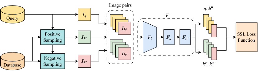
Figure 1: VG-SSL Framework Overview. Initially, query images $I_{q}$ are randomly sampled, and corresponding positive database images $I_{k^{p}}$ are identified. Negative database images $I_{k^{n}}$ are randomly selected from the database excluding $I_{k^{p}}$. Image pairs are built using query-positive pairs ($I_{q}$, $I_{k^{p}}$) and identical negative pairs ($I_{k^{n}}$, $I_{k^{n}}$) with a database negative ratio of $\eta$. Following this, we utilize feature extractor $F$ to extract features and generate embeddings $q$, $k^{p}$, and $k_{n}$. Depending on the specific SSL loss function in use, $L_{2}$ normalization may be applied to yield normalized embeddings $\tilde{q}$, $\tilde{k}^{p}$, and $\tilde{k}_{n}$. Finally, we utilize the SSL loss function with these embeddings to train $F$.

where $d_{1}$ is a scalar of the margin as a hyperparameter. This loss function optimizes to make the distance between $q$ and $k^{p}$ lower than the distance between $q$ and $k^{n}$ but will be zero if the difference is greater than the margin.

InfoNCE Loss. InfoNCE Loss [36] is used in contrastive learning SSL methods [11, 25, 12]. The intuition of this loss is to reduce the embedding distance between positive pairs and increase the embedding distance to all other pairs. The loss function is formulated as

$$\mathcal{L}_{\textrm{InfoNCE}}=\frac{1}{N}\sum_{b=1}^{N}\log\frac{\exp(\tilde{q_{b}}\cdot\tilde{k^{p}_{b}}/\tau)}{\sum_{i=1,i\neq b}^{N}\exp(\tilde{q_{b}}\cdot\tilde{k^{p}_{i}}/\tau)},$$ (2)

where $\tau$ is the temperature parameter. The symmetric version of this loss is to swap the input images, calculate the loss twice and average it.

Embedding Prediction Loss. Embedding Prediction Loss is used in self-distillation methods [22, 13]. The aim of the loss function is to predict the common representation between the teacher embedding and the student embedding. The loss function is formulated as

$$\mathcal{L}_{\textrm{EmbPred}}=\frac{1}{N}\sum_{b=1}^{N}[2-2||p(\tilde{q_{b}})||_{2}\cdot\textrm{stopgrad}(\tilde{k^{p}_{b}})],$$ (3)

where $p(\cdot)$ is a shallow MLP to predict the teacher embedding and $\textrm{stopgrad}(\cdot)$ means the gradient is not backpropagated to the teacher model. Similar to InfoNCE (Equation 2), the symmetric version of this loss swaps the input images and calculates the average loss.

Cross-correlation Loss. Barlow Twins (BT) [48] introduces the Cross-correlation Loss. The first step is to build a cross-correlation matrix. It is defined as

$$C_{ij}=\frac{\sum_{b=1}^{N}q_{b,i}k^{p}_{b,j}}{\sqrt{\sum_{b=1}^{N}(q_{b,i})^{2}}\sqrt{\sum_{b=1}^{N}(k^{p}_{b,j})^{2}}},$$ (4)

where $i,j$ are the index of elements of the embedding, and $C$ is a square cross-correlation matrix range from -1 (negative correlation) to 1 (positive correlation). Then, the BT loss $L_{\textrm{BT}}$ is calculated as

$$\mathcal{L}_{\textrm{BT}}=\sum_{i=1}^{D}(1-C_{ii})^{2}+\lambda\sum_{i=1}^{D}\sum_{j=1,j\neq i}^{D}C_{ij},$$ (5)

where $\lambda$ is the weight of the off-diagonal term as a hyperparameter. The intuition of this loss is to enforce the same element of embeddings positively correlated and the different elements of embeddings uncorrelated to maximize contained information.

VIC Regularization Loss. VIC Regularization (VICReg) Loss [6] is inspired by BT Loss and explicitly defines the invariance (the first row), variance (the second row), and covariance (the third row) terms of the elements of the embeddings as

$$\begin{split}\mathcal{L}_{\textrm{VICReg}}&=\frac{\lambda_{1}}{ND}\sum_{b=1}^{N}\sum_{i=1}^{D}\|q_{b,i}-k^{p}_{b,i}\|_{2}^{2}\\ &+\frac{\lambda_{2}}{D}\sum_{i=1}^{D}\left[\max\{d_{2}-\textrm{std}_{i}(q),0\}+\max\{d_{2}-\textrm{std}_{i}(k^{p}),0\}\right]\\ &+\frac{\lambda_{3}}{D}\sum_{i=1}^{D}\sum_{j=1,j\neq i}^{D}\left[\textrm{cov}^{2}_{ij}(q)+\textrm{cov}^{2}_{ij}(k^{p})\right],\end{split}$$ (6)

where $\lambda_{1},\lambda_{2},\lambda_{3},d_{2}$ are hyperparameters, $\textrm{std}_{i}(q)$ is the standard deviation of the $i$-th element of $q$ over the batch, and $\textrm{cov}_{ij}(q)$ is the element of the $i$-th row and $j$-th column of the covariance matrix of $q$ over the batch. This loss function attempts to decorrelate the elements of the embedding by reducing the off-diagonal elements of the covariance matrix to zeros. It also uses the variance term to maximize the standard deviation of the element of embeddings over the batch with a margin $d_{2}$.

Remarks for Cross-correlation Loss and VICReg Loss. In our preliminary experiments, we noticed that $L_{2}$ normalization for $q_{b}$ and $k^{p}_{b}$ hinders the performance of models utilizing Cross-correlation Loss and prevents convergence for models employing VICReg Loss. This suggests that feature-wise $L_{2}$ normalization may interfere with the batch-wise computation of cross-correlation and covariance matrices. Consequently, we use unnormalized embeddings $q_{b}$ and $k^{p}_{b}$ for both loss functions.

3.2 Database Negative Ratio

We notice that for original SSL methods, the loss functions solely focus on query embeddings $q_{b}$ and positive embeddings $k^{p}_{b}$. However, in VG tasks, a considerable number of negative samples lack corresponding query samples, leading to their exclusion from the SSL training process and ultimately resulting in degraded VG performance. To address this issue, we introduce a hyperparameter called Database Negative Ratio $\eta$. We denote the database as $I_{k}$. For each epoch, we sample $m_{q}$ query images and obtain $m_{k}$ positive images $I_{k^{p}}$. From the negative images $I_{k^{n}}=I_{k}\setminus I_{k^{p}}$, we randomly sample $m^{n}_{k}=\eta m_{q}$ negative images and built identical image pairs. Consequently, our new sampling method combines both query-positive pairs ($I_{q}$, $I_{k^{p}}$) and identical negative pairs ($I_{k^{n}}$, $I_{k^{n}}$) with the ratio $\eta$ during training. Our results indicate that certain SSL methods can enhance VG performance when the database negative ratio $\eta=1$; however, some methods will have the model collapse issue when $\eta$ is large.

3.3 Training Time Complexity and Memory Usage

In this section, we compare the time complexity and memory usage between VG-SSL and the baseline Triplet method with HNM [9] during training. The preparation time for training data can be divided into two parts: Part 1: the extraction phase, which involves generating embeddings from images, and Part 2: the matching phase, where query embeddings match database embeddings. Subsequently, we can construct pairs or triplets and proceed with the training process. When full database HNM is employed, the extraction time complexity and memory usage are proportional to $O(\#I_{q}+\#I_{k})$, while the matching time complexity is proportional to $O(\#I_{q}\#I_{k})$. This denotes substantial computational and memory demands for HNM. On the other hand, with partial database HNM, the extraction time complexity and memory usage are proportional to $O(\#I_{q}+\#I_{k^{n}}+\#I_{k^{p}})$, and the matching time complexity is proportional to $O(\#I_{q}\#I_{k^{n}}+\#I_{q}\#I_{k^{p}})$. This configuration considerably reduces resource requirements compared to full mining. However, a decline in performance may be observed when $\#I_{k^{n}}$ decreases. In contrast, our framework eliminates the need for HNM. The extraction time complexity and memory usage become proportional to $O(\#I_{q}+\#I_{k^{p}})$, and the matching time complexity is proportional to $O(\#I_{q}\#I_{k^{p}})$. This configuration leads to a further reduction in resource utilization while ensuring a performance level comparable to the partial mining case.

4 Experiment Setup

4.1 Datasets and Metrics

For our experiments, we are using five public VG datasets: Pitts30k [42], MSLS [45], Tokyo 24/7 [41], Eynsham [17], and St. Lucia [33]. We utilize MSLS to train and demonstrate the effectiveness of our methods trained on large datasets. Note that the validation set of MSLS is used for testing because the ground truth of the test set is not publicly available. Pitts30k and the database of Tokyo 24/7 are sourced from Google Street View, while the query images of Tokyo 24/7 are captured by a smartphone. MSLS, Eynsham, and St. Lucia datasets are acquired with a front-view camera mounted on a car. For Pitts30k, MSLS, Eynsham, and St.Lucia, the aspect ratio and resolution of query images and database images are consistent. However, this consistency is not guaranteed in Tokyo 24/7, because the query images may adjust the aspect ratio. For simplicity, we resize the test images of Tokyo 24/7 to $480\times 640$ (H$\times$W), as well as the training images of MSLS.

We evaluate all of our experiments using the Recall@N (R@N) metric. This measures the percentage of query images for which the top-N prediction falls within a specified radius threshold from the actual geolocation. The higher recall value means more accurate VG results. Our primary focus is on the Recall@1 metric, and we have set the threshold at 25 meters to ensure a consistent comparison with other studies in the field of VG.

4.2 Implementation Details

In our work, we follow a part of the settings in the baseline VG pipeline [9] and make modifications based on different SSL methods adapted into VG. The training image size is $480\times 640$. With a batch size $B$ of $64$, each batch consists of $64$ image pairs. We use Adam optimizer [30] with learning rates $1e^{-5}$ (SimCLR and MoCov2) and $1e^{-4}$ (BYOL, SimSiam, BT, and VICReg), and weight decay $1e^{-6}$. We conduct our experiments mainly with ResNet-50 [26] as the local feature extractor $F_{l}$ and NetVLAD [4] as the global aggregation module $F_{g}$. We use ImageNet [18] pre-trained weights and extract the features from conv4_x of ResNet-50. We run for $24$ hours with approximately $250$ epochs, and each epoch iterates $5000$ queries. During training, we define images as positive samples if they are within the $10$ m radius of the query images and negative samples if they are beyond the $25$ m radius of the query images. Following the origin settings of SSL methods, the projection head of SimCLR and MoCov2 have no batch normalization, and BYOL, SimSiam, BT, and VICReg have batch normalization. The models are primarily trained with the batch size of $64$ in one NVIDIA-A100-80GB GPU. The pipelines are implemented using Pytorch-lightning [19].

5 Results

5.1 Optimal Settings for SSL Methods

In this section, we summarize the optimal settings for different SSL methods in the VG-SSL framework and compare our results with the baseline VG model with Hard Negative Mining (HNM) from [9]. The naming convention in Tables 2-4 for Training Strategies is hyphen-separated and structured as follows: The first segment is the names of SSL methods or Triplet (Baseline). The second segment is the projection methods, including PCA or FC (Fully-Connected) layers. If the methods use FC, then the number of FC layers follows the term FC. The third segment is the dimensionality of the embeddings. The fourth segment is the database negative ratio. For example, "SimCLR-FC-1-2048-1" denotes the strategy using the SimCLR method with a 1-layer projection head, an output dimension of 2048, and a database negative ratio of 1. The "Triplet" strategy uses HNM by default, unless "Random" follows the strategy, which denotes the use of random sampling for negative samples. Standard deviations across multiple runs and the comparison of different batch sizes are shown in the Appendix.

In Table 2, we show the results of optimal settings divided by different dimensionality of embeddings. Tokyo 24/7 results from the original paper are not presented here due to the unique resize strategy employed specifically for the dataset in that study. In contrast, our methods consistently resize to a fixed image size for simplicity. For a fair comparison, we have reproduced the Tokyo 24/7 results utilizing our own fixed-size resize strategy. The results show that among SSL methods, BT-FC-2-4096-1 has the best performance with $D=4096$, and SimCLR-FC-2-2048-1 and MoCov2-FC-2-2048-1 outperform other SSL methods with $D=2048$. Notably, the aforementioned methods have comparable performance to the Triplet strategy even when the Triplet strategy employs HNM and utilizes a significantly larger feature dimension of $65536$. Moreover, these methods substantially outperform Triplet-Random, further highlighting the effectiveness of SSL methods without HNM.

Table 2: Comparison of optimal settings in VG-SSL with previous state-of-the-art results. $\ast$ the results are reproduced by our retrained model with the original settings. The bold value is the best value and the underline value is the second best value. SimCLR, BT, and VICReg use a batch size of 256. MoCov2, BYOL, and SimSiam are trained with batch size = 64.

Training Strategies	Feature Dim	R@1 Pitts30k	R@1 MSLS	R@1 Tokyo24/7	R@1 Eynsham	R@1 St.Lucia
Triplet [9]	65535	80.9	76.9	-	87.2	93.8
Triplet (Repro.)		78.6	77.9	45.7	86.0	94.8
Triplet-Random [9]		74.9	63.6	-	85.5	80.9
Triplet-PCA-4096 (Repro.)	4096	76.7	77.1	43.3	85.2	94.7
BT-FC-2-4096-1		76.8	77.9	43.8	84.2	91.3
VICReg-FC-2-4096-1		72.0	74.2	35.7	81.7	86.7
Triplet-PCA-2048 [9]	2048	78.5	75.4	-	85.8	93.4
Triplet-PCA-2048 (Repro.)		75.8	76.7	40.7	84.8	94.6
SimCLR-FC-1-2048-1		75.2	76.6	44.3	85.6	91.2
MoCov2-FC-1-2048-1		76.2	74.2	47.0	84.8	89.1
BYOL-FC-2-2048-0.25		76.0	75.7	43.9	84.3	90.5
SimSiam-FC-2-2048-0.25		69.2	69.3	35.7	81.9	86.5

5.2 Ablation study

In this section, we conduct the ablation study on the following factors: Database Negative Ratio $\eta$, Number of Projection Layers $L$, and Dimensionality of Embeddings $D$. We use a batch size of $64$ by default for the ablation study.

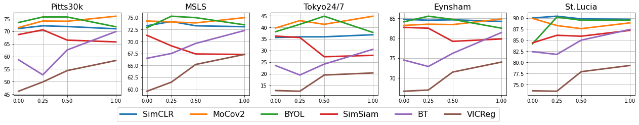
Figure 2: The comparison of different database negative ratios $\eta$ across multiple runs. The X-axis is the database negative ratio $\eta$, and the Y-axis is the R@1 values.

5.2.1 Database Negative Ratio

Fig. 2 examines how varying the database negative ratio $\eta$ impacts the VG performance across different SSL methods. We conduct experiments with $\eta$ values of $0$, $0.25$, $0.5$, and $1$. With MoCov2, BT, and VICReg, we mostly observed that the best VG performance is achieved with the highest database negative ratio ($\eta=1$), except for MoCov2 in St. Lucia dataset. Conversely, SimCLR’s performance shows no significant changes across different $\eta$ values. On the other hand, BYOL exhibits peak performance at $\eta=0.25$ or $0.5$. SimSiam shows peak performance at $\eta=0$ or $0.25$. A higher $\eta$ seems to impair the VG performance of these methods.

Discussion. As detailed in Section 3.2, the primary advantage of sampling database negatives is to utilize those negatives whose corresponding query images do not exist. However, as we use the negatives as their respective query images, there is a risk that the identical pairs might cause the model to collapse, thereby degrading the training performance. This collapse is not observed in SimCLR, MoCov2, BT, and VICReg at $\eta=1$. This occurs because the identical negative pairs do not fundamentally influence the calculation of InfoNCE Loss, Cross-correlation Loss, and VICReg Loss. Conversely, it only results in a portion of the positive pair becoming ineffective within the loss function calculation. However, the collapse is quite obvious in the case of BYOL and SimSiam when $\eta$ is large. The explanation is that when trained with identical pairs, the predictor tends to learn identical mapping instead of the common representation of paired images. This issue is particularly severe for SimSiam as it replicates the online encoder as the target encoder, rather than using a momentum target encoder. Therefore, to optimize the performance of BYOL and SimSiam, the value of $\eta$ should be carefully adjusted to a point between no database negatives and model collapse.

Table 3: Comparison of different numbers of projection layers $L$

Training Strategies	# Proj layers	R@1 Pitts30k	R@1 MSLS	R@1 Tokyo24/7	R@1 Eynsham	R@1 St.Lucia
SimCLR-FC-1-2048-1	1	71.6	72.5	38.3	84.3	89.6
MoCov2-FC-1-2048-1		76.2	74.2	47.0	84.8	89.1
BYOL-FC-1-2048-0.25		61.9	61.0	30.9	76.8	75.9
SimSiam-FC-1-2048-0.25		23.2	18.2	3.8	36.0	25.7
BT-FC-1-2048-1		62.0	69.8	29.2	73.8	84.4
VICReg-FC-1-2048-1		27.6	41.2	6.2	43.5	51.2
SimCLR-FC-2-2048-1	2	63.9	69.1	31.0	81.3	86.5
MoCov2-FC-2-2048-1		69.2	71.9	35.1	80.9	85.9
BYOL-FC-2-2048-0.25		76.0	75.7	43.9	84.3	90.5
SimSiam-FC-2-2048-0.25		69.2	69.3	35.7	81.9	86.5
BT-FC-2-2048-1		70.5	72.6	32.1	80.5	86.2
VICReg-FC-2-2048-1		58.3	67.5	23.2	72.3	78.6
BYOL-FC-3-2048-0.25	3	67.4	71.5	33.8	81.1	85.1
SimSiam-FC-3-2048-0.25		56.8	65.7	21.8	75.2	78.6
BT-FC-3-2048-1		55.2	67.5	21.0	73.8	79.9
VICReg-FC-3-2048-1		42.4	58.8	12.1	66.0	71.3

5.2.2 Number of Projection Layers

In Table 3, we explore the number of projection layers $L$ for various SSL methods. The baseline model [9] employs PCA to generate the embeddings with the specified dimensionality. In contrast, our VG-SSL method uses FC layers for this projection. The number of projection layers ($L$) significantly influences the model’s convergence. With a single projection layer, the projection head essentially performs a linear projection onto the embedding, while with two or more layers, the module is capable of executing non-linear projection.

As per our findings in Table 3, the optimal number of projection layers for SimCLR and MoCov2 is 1. For BYOL, SimSiam, BT, and VICReg, the optimal number of layers is 2. We note that when $L=1$, SimSiam shows model collapse, and BYOL, BT, and VICReg deteriorate. These observations suggest that linear projection is unsuitable for these methods, a conclusion that aligns with the findings in the corresponding original papers [22, 13, 48, 6].

Discussion. A key insight from Table 3 is that increasing the number of projection layers does not necessarily improve VG performance, as common SSL methods exhibit on classification tasks. Specifically, original SimCLR [11] and MoCov2 [12] demonstrate improved classification performance with non-linear projection, while our results indicate that linear projection yields better VG performance for these two methods. Meanwhile, original BT [48] and VICReg [6] prefer $3$ projection layers, while our results show $2$ projection layers yield better VG performance for these methods. We note two major differences between the original application of SSL methods and our approach: 1) We utilize projected embeddings for VG tasks, while the original methods discard the projector and employ the un-projected embeddings for downstream tasks; 2) We use a batch size of $64$, which is lower compared to typical SSL method usage. This change can potentially explain the aforementioned observed difference.

5.2.3 Dimensionality of Embeddings

Table 4 shows the comparison of SSL methods with different dimensionality of embeddings $D$. One notable observation is that both BT and VICReg methods exhibit substantial performance improvements as $D$ increases. In contrast, other methods demonstrate less sensitivity to changes in $D$. This observation aligns with the requirement of large dimensionality of embeddings in the original papers for BT and VICReg [48, 6]. Additionally, it is significant to note that SimCLR, MoCov2, and BYOL maintain comparable performance even when $D$ is reduced to 1024. This suggests the potential to further reduce the dimensionality, which may result in a modest decrease in performance but concurrently enhance efficiency and reduce memory usage.

Table 4: Comparison of different dimensionalities of embeddings $D$

Training Strategies	Feature Dim	R@1 Pitts30k	R@1 MSLS	R@1 Tokyo24/7	R@1 Eynsham	R@1 St.Lucia
SimCLR-FC-4096-1	4096	71.6	72.9	39.6	84.1	90.2
MoCov2-FC-4096-1		76.2	74.5	46.7	84.9	89.5
BYOL-FC-2-4096-0.25		73.4	74.6	42.9	84.6	88.7
SimSiam-FC-2-4096-0.25		68.2	73.6	33.9	80.6	89.0
BT-FC-2-4096-1		73.6	73.8	37.7	82.6	88.4
VICReg-FC-2-4096-1		61.8	69.8	25.1	74.3	81.3
SimCLR-FC-1-2048-1	2048	71.6	72.5	38.3	84.3	89.6
MoCov2-FC-1-2048-1		76.2	74.2	47.0	84.8	89.1
BYOL-FC-2-2048-0.25		76.0	75.7	43.9	84.3	90.5
SimSiam-FC-2-2048-0.25		69.2	69.3	35.7	81.9	86.5
BT-FC-2-2048-1		70.5	72.6	32.1	80.5	86.2
VICReg-FC-2-2048-1		58.3	67.5	23.2	72.3	78.6
SimCLR-FC-1-1024-1	1024	70.6	72.7	39.7	84.1	90.1
MoCov2-FC-1-1024-1		75.2	73.8	44.8	84.5	88.7
BYOL-FC-2-1024-0.25		73.4	74.6	42.9	84.6	88.7
SimSiam-FC-2-1024-0.25		67.3	69.1	31.8	79.8	85.9
BT-FC-2-1024-1		60.8	69.2	23.5	74.3	82.2
VICReg-FC-1024-1		47.7	61.9	16.4	64.3	72.0

6 Conclusions and Discussions

In this work, we presented an innovative VG-SSL framework that integrates six popular SSL methods into VG tasks, thereby eliminating the necessity for HNM. Our observations suggest that BT, SimCLR, and MoCov2 are preferred methods for representation learning within large VG datasets, and exhibit VG performance comparable to the Triplet method with HNM. Due to resource limitations, we have employed a much smaller batch size than typically used in SSL pretraining, which may negatively affect the performance. Nevertheless, we assert that the VG task can serve as a robust benchmark for the evaluation of various SSL methods by using existing and diverse VG datasets. In the future, we aim to expand our framework by incorporating additional SSL methods and examining the impact of augmentation and image size on its performance.

Appendix A Extended Results

In this section, we show the results of 3 runs with different random seeds to analyze the mean and standard deviation of Recall@1 (R@1) values. Additionally, we include the comparison of different batch sizes $N$ in this section. We will update the results in the main paper for the final print.

A.1 Optimal Settings

The results of the optimal settings across multiple runs are shown in Table 5. From this table, the recommended SSL methods for VG are BT-FC-2-4096-1, SimCLR-FC-2-2048-1, and MoCov2-FC-2-2048-1, which is consistent with our conclusion. And we find that BYOL-FC-2-2048-0.25 also shows comparable performance with the above methods.

Table 5: Comparison of optimal settings in VG-SSL and the baseline model with HNM across multiple runs. SimCLR, BT, and VICReg use a batch size of 256. MoCov2, BYOL, and SimSiam are trained with batch size = 64.

Training Strategies	Feature Dim	R@1 Pitts30k	R@1 MSLS	R@1 Tokyo24/7	R@1 Eynsham	R@1 St.Lucia
Triplet	65535	80.9 $\pm$ 0.0	76.9 $\pm$ 0.2	-	87.2 $\pm$ 0.3	93.8 $\pm$ 0.2
Triplet (Repro.)		78.6 $\pm$ 0.5	77.9 $\pm$ 0.2	45.7 $\pm$ 3.6	86.0 $\pm$ 0.3	94.8 $\pm$ 0.5
Triplet-Random		74.9 $\pm$ 0.4	63.6 $\pm$ 1.3	-	85.5 $\pm$ 0.2	80.9 $\pm$ 0.4
Triplet-PCA-4096 (Repro.)	4096	76.7 $\pm$ 1.1	77.1 $\pm$ 0.2	43.3 $\pm$ 2.4	85.2 $\pm$ 0.5	94.7 $\pm$ 0.7
BT-FC-2-4096-1		76.8 $\pm$ 0.2	77.9 $\pm$ 0.5	43.8 $\pm$ 1.1	84.2 $\pm$ 0.5	91.3 $\pm$ 0.3
VICReg-FC-2-4096-1		72.0 $\pm$ 1.0	74.2 $\pm$ 0.4	35.7 $\pm$ 1.5	81.7 $\pm$ 0.9	86.7 $\pm$ 0.5
Triplet-PCA-2048	2048	78.5 $\pm$ 0.2	75.4 $\pm$ 0.2	-	85.8 $\pm$ 0.3	93.4 $\pm$ 0.4
Triplet-PCA-2048 (Repro.)		75.8 $\pm$ 1.1	76.7 $\pm$ 0.3	40.7 $\pm$ 2.4	84.8 $\pm$ 0.5	94.6 $\pm$ 0.7
SimCLR-FC-1-2048-1		75.2 $\pm$ 0.6	76.6 $\pm$ 0.5	44.3 $\pm$ 2.4	85.6 $\pm$ 0.0	91.2 $\pm$ 0.6
MoCov2-FC-1-2048-1		76.2 $\pm$ 0.9	74.2 $\pm$ 0.9	47.0 $\pm$ 4.1	84.8 $\pm$ 0.0	89.1 $\pm$ 0.2
BYOL-FC-2-2048-0.25		76.0 $\pm$ 0.4	75.7 $\pm$ 0.4	43.9 $\pm$ 2.3	84.3 $\pm$ 1.2	90.5 $\pm$ 0.9
SimSiam-FC-2-2048-0.25		69.2 $\pm$ 1.4	69.3 $\pm$ 0.5	35.7 $\pm$ 1.4	81.9 $\pm$ 0.5	86.5 $\pm$ 0.4

A.2 Database Negative Ratio

The comparison of different database negative ratios $\eta$ across multiple runs is shown in Table 6. We can observe that SimCLR, MoCov2, BT, and VICReg have the best performance when $\eta=1$. BYOL has peak performance when $\eta=0.25$ or $0.5$, while SimSiam has peak performance when $\eta=0$ or $0.25$.

Table 6: Comparison of different database negative ratios $\eta$ across multiple runs

Training Strategies	Negative Ratio	R@1 Pitts30k	R@1 MSLS	R@1 Tokyo24/7	R@1 Eynsham	R@1 St.Lucia
SimCLR-FC-1-2048-0	0	71.7 $\pm$ 0.9	73.9 $\pm$ 0.5	38.4 $\pm$ 3.9	84.8 $\pm$ 0.4	90.1 $\pm$ 0.2
MoCov2-FC-1-2048-0		72.4 $\pm$ 0.9	73.9 $\pm$ 0.3	39.3 $\pm$ 0.5	83.5 $\pm$ 0.3	90.1 $\pm$ 0.2
BYOL-FC-2-2048-0		73.0 $\pm$ 0.5	72.7 $\pm$ 0.2	41.0 $\pm$ 3.5	84.1 $\pm$ 0.2	86.1 $\pm$ 1.7
SimSiam-FC-2-2048-0		70.7 $\pm$ 2.0	72.0 $\pm$ 0.7	37.3 $\pm$ 1.8	83.0 $\pm$ 0.3	86.1 $\pm$ 2.6
BT-FC-2-2048-0		57.4 $\pm$ 0.8	66.4 $\pm$ 0.4	20.3 $\pm$ 4.0	73.4 $\pm$ 1.7	81.6 $\pm$ 0.7
VICReg-FC-2-2048-0		50.2 $\pm$ 4.4	60.3 $\pm$ 0.6	13.2 $\pm$ 0.7	68.0 $\pm$ 2.2	74.8 $\pm$ 1.2
SimCLR-FC-1-2048-0.25	0.25	71.7 $\pm$ 0.5	72.5 $\pm$ 1.7	37.4 $\pm$ 1.8	84.4 $\pm$ 0.1	89.3 $\pm$ 1.6
MoCov2-FC-1-2048-0.25		74.5 $\pm$ 0.5	74.2 $\pm$ 0.2	43.5 $\pm$ 2.4	83.9 $\pm$ 0.4	88.9 $\pm$ 0.8
BYOL-FC-2-2048-0.25		76.0 $\pm$ 0.4	75.7 $\pm$ 0.4	43.9 $\pm$ 2.3	84.3 $\pm$ 1.2	90.5 $\pm$ 0.9
SimSiam-FC-2-2048-0.25		69.2 $\pm$ 1.4	69.3 $\pm$ 0.5	35.7 $\pm$ 1.4	81.9 $\pm$ 0.5	86.5 $\pm$ 0.4
BT-FC-2-2048-0.25		56.7 $\pm$ 3.8	68.2 $\pm$ 0.6	22.0 $\pm$ 2.3	73.5 $\pm$ 0.8	81.8 $\pm$ 1.9
VICReg-FC-2-2048-0.25		52.8 $\pm$ 2.5	62.5 $\pm$ 1.0	16.3 $\pm$ 3.5	70.2 $\pm$ 2.8	75.9 $\pm$ 2.1
SimCLR-FC-1-2048-0.5	0.5	71.1 $\pm$ 0.9	71.9 $\pm$ 1.2	36.4 $\pm$ 0.6	84.4 $\pm$ 0.2	89.9 $\pm$ 0.7
MoCov2-FC-1-2048-0.5		75.0 $\pm$ 0.9	74.5 $\pm$ 0.5	42.8 $\pm$ 1.3	84.1 $\pm$ 0.6	89.0 $\pm$ 1.5
BYOL-FC-2-2048-0.5		76.1 $\pm$ 0.3	75.6 $\pm$ 0.5	46.2 $\pm$ 1.2	84.4 $\pm$ 0.4	90.5 $\pm$ 1.4
SimSiam-FC-2-2048-0.5		67.0 $\pm$ 1.4	68.4 $\pm$ 1.0	29.8 $\pm$ 3.1	79.8 $\pm$ 0.9	85.2 $\pm$ 1.4
BT-FC-2-2048-0.5		63.0 $\pm$ 1.1	70.3 $\pm$ 0.6	27.1 $\pm$ 2.7	77.1 $\pm$ 0.8	84.9 $\pm$ 0.7
VICReg-FC-2-2048-0.5		52.6 $\pm$ 1.6	64.4 $\pm$ 0.7	18.6 $\pm$ 2.2	69.2 $\pm$ 2.1	77.6 $\pm$ 1.3
SimCLR-FC-1-2048-1	1	71.6 $\pm$ 1.1	72.5 $\pm$ 1.0	38.3 $\pm$ 1.3	84.3 $\pm$ 0.1	89.6 $\pm$ 0.1
MoCov2-FC-1-2048-1		76.2 $\pm$ 0.9	74.2 $\pm$ 0.9	47.0 $\pm$ 4.1	84.8 $\pm$ 0.0	89.1 $\pm$ 0.2
BYOL-FC-2-2048-1		71.6 $\pm$ 1.8	73.0 $\pm$ 0.6	36.9 $\pm$ 1.8	80.6 $\pm$ 3.5	89.3 $\pm$ 0.5
SimSiam-FC-2-2048-1		68.7 $\pm$ 2.6	67.5 $\pm$ 0.2	30.5 $\pm$ 2.3	80.8 $\pm$ 1.1	86.8 $\pm$ 0.8
BT-FC-2-2048-1		70.5 $\pm$ 1.5	72.6 $\pm$ 0.6	32.1 $\pm$ 1.8	80.5 $\pm$ 0.8	86.2 $\pm$ 1.2
VICReg-FC-2-2048-1		58.3 $\pm$ 0.3	67.5 $\pm$ 0.7	23.2 $\pm$ 2.5	72.3 $\pm$ 1.3	78.6 $\pm$ 1.4

A.3 Number of Projection Layers

The comparison of different projection layers $L$ across multiple runs is shown in Table 7. We can observe that BYOL, SimSiam, BT, and VICReg have the best performance when $L=2$, while SimCLR and MoCov2 have peak performance when $L=1$.

Table 7: Comparison of different numbers of projection $L$ across multiple runs

Training Strategies	# Proj layers	R@1 Pitts30k	R@1 MSLS	R@1 Tokyo24/7	R@1 Eynsham	R@1 St.Lucia
SimCLR-FC-1-2048-1	1	71.6 $\pm$ 1.1	72.5 $\pm$ 1.0	38.3 $\pm$ 1.3	84.3 $\pm$ 0.1	89.6 $\pm$ 0.1
MoCov2-FC-1-2048-1		76.2 $\pm$ 0.9	74.2 $\pm$ 0.9	47.0 $\pm$ 4.1	84.8 $\pm$ 0.0	89.1 $\pm$ 0.2
BYOL-FC-1-2048-0.25		61.9 $\pm$ 12.3	61.0 $\pm$ 15.6	30.9 $\pm$ 9.4	76.8 $\pm$ 7.3	75.9 $\pm$ 14.3
SimSiam-FC-1-2048-0.25		23.2 $\pm$ 5.3	18.2 $\pm$ 7.9	3.8 $\pm$ 2.1	36.0 $\pm$ 9.3	25.7 $\pm$ 8.8
BT-FC-1-2048-1		62.0 $\pm$ 2.1	69.8 $\pm$ 0.5	29.2 $\pm$ 1.4	73.8 $\pm$ 3.7	84.4 $\pm$ 0.9
VICReg-FC-1-2048-1		27.6 $\pm$ 2.4	41.2 $\pm$ 2.4	6.2 $\pm$ 1.4	43.5 $\pm$ 3.6	51.2 $\pm$ 1.8
SimCLR-FC-2-2048-1	2	63.9 $\pm$ 1.0	69.1 $\pm$ 1.2	31.0 $\pm$ 1.5	81.3 $\pm$ 0.5	86.5 $\pm$ 0.7
MoCov2-FC-2-2048-1		69.2 $\pm$ 1.7	71.9 $\pm$ 0.3	35.1 $\pm$ 1.8	80.9 $\pm$ 1.1	85.9 $\pm$ 0.3
BYOL-FC-2-2048-0.25		76.0 $\pm$ 0.4	75.7 $\pm$ 0.4	43.9 $\pm$ 2.3	84.3 $\pm$ 1.2	90.5 $\pm$ 0.9
SimSiam-FC-2-2048-0.25		69.2 $\pm$ 1.4	69.3 $\pm$ 0.5	35.7 $\pm$ 1.4	81.9 $\pm$ 0.5	86.5 $\pm$ 0.4
BT-FC-2-2048-1		70.5 $\pm$ 1.5	72.6 $\pm$ 0.6	32.1 $\pm$ 1.8	80.5 $\pm$ 0.8	86.2 $\pm$ 1.2
VICReg-FC-2-2048-1		58.3 $\pm$ 0.3	67.5 $\pm$ 0.7	23.2 $\pm$ 2.5	72.3 $\pm$ 1.3	78.6 $\pm$ 1.4
BYOL-FC-3-2048-0.25	3	67.4 $\pm$ 1.7	71.5 $\pm$ 0.4	33.8 $\pm$ 2.4	81.1 $\pm$ 0.2	85.1 $\pm$ 1.7
SimSiam-FC-3-2048-0.25		56.8 $\pm$ 5.1	65.7 $\pm$ 0.6	21.8 $\pm$ 3.1	75.2 $\pm$ 0.4	78.6 $\pm$ 2.0
BT-FC-3-2048-1		55.2 $\pm$ 0.5	67.5 $\pm$ 0.8	21.0 $\pm$ 1.3	73.8 $\pm$ 0.7	79.9 $\pm$ 1.0
VICReg-FC-3-2048-1		42.4 $\pm$ 2.1	58.8 $\pm$ 0.2	12.1 $\pm$ 1.8	66.0 $\pm$ 2.2	71.3 $\pm$ 1.3

A.4 Dimensionality of Embeddings

The comparison of different dimensionality of embeddings $D$ across multiple runs is shown in Table 8. We can observe that both BT and VICReg methods exhibit substantial performance improvements as $D$ increases. In contrast, other methods demonstrate less sensitivity to changes in $D$.

Table 8: Comparison of different dimensionalities of embeddings $D$ across multiple runs

Training Strategies	Feature Dim	R@1 Pitts30k	R@1 MSLS	R@1 Tokyo24/7	R@1 Eynsham	R@1 St.Lucia
SimCLR-FC-4096-1	4096	71.6 $\pm$ 0.7	72.9 $\pm$ 0.3	39.6 $\pm$ 1.3	84.1 $\pm$ 0.5	90.2 $\pm$ 0.6
MoCov2-FC-4096-1		76.2 $\pm$ 0.6	74.5 $\pm$ 1.2	46.7 $\pm$ 0.4	84.9 $\pm$ 0.2	89.5 $\pm$ 0.3
BYOL-FC-2-4096-0.25		73.4 $\pm$ 0.6	74.6 $\pm$ 0.4	42.9 $\pm$ 1.8	84.6 $\pm$ 0.1	88.7 $\pm$ 2.5
SimSiam-FC-2-4096-0.25		68.2 $\pm$ 1.9	73.6 $\pm$ 1.0	33.9 $\pm$ 2.6	80.6 $\pm$ 1.1	89.0 $\pm$ 2.2
BT-FC-2-4096-1		73.6 $\pm$ 2.2	73.8 $\pm$ 0.5	37.7 $\pm$ 0.3	82.6 $\pm$ 1.1	88.4 $\pm$ 1.2
VICReg-FC-2-4096-1		61.8 $\pm$ 2.7	69.8 $\pm$ 0.7	25.1 $\pm$ 3.0	74.3 $\pm$ 1.3	81.3 $\pm$ 0.9
SimCLR-FC-1-2048-1	2048	71.6 $\pm$ 1.1	72.5 $\pm$ 1.0	38.3 $\pm$ 1.3	84.3 $\pm$ 0.1	89.6 $\pm$ 0.1
MoCov2-FC-1-2048-1		76.2 $\pm$ 0.9	74.2 $\pm$ 0.9	47.0 $\pm$ 4.1	84.8 $\pm$ 0.0	89.1 $\pm$ 0.2
BYOL-FC-2-2048-0.25		76.0 $\pm$ 0.4	75.7 $\pm$ 0.4	43.9 $\pm$ 2.3	84.3 $\pm$ 1.2	90.5 $\pm$ 0.9
SimSiam-FC-2-2048-0.25		69.2 $\pm$ 1.4	69.3 $\pm$ 0.5	35.7 $\pm$ 1.4	81.9 $\pm$ 0.5	86.5 $\pm$ 0.4
BT-FC-2-2048-1		70.5 $\pm$ 1.5	72.6 $\pm$ 0.6	32.1 $\pm$ 1.8	80.5 $\pm$ 0.8	86.2 $\pm$ 1.2
VICReg-FC-2-2048-1		58.3 $\pm$ 0.3	67.5 $\pm$ 0.7	23.2 $\pm$ 2.5	72.3 $\pm$ 1.3	78.6 $\pm$ 1.4
SimCLR-FC-1-1024-1	1024	70.6 $\pm$ 0.8	72.7 $\pm$ 0.6	39.7 $\pm$ 1.5	84.1 $\pm$ 0.3	90.1 $\pm$ 0.2
MoCov2-FC-1-1024-1		75.2 $\pm$ 0.3	73.8 $\pm$ 1.0	44.8 $\pm$ 1.6	84.5 $\pm$ 0.2	88.7 $\pm$ 1.5
BYOL-FC-2-1024-0.25		73.4 $\pm$ 0.6	74.6 $\pm$ 0.4	42.9 $\pm$ 1.8	84.6 $\pm$ 0.1	88.7 $\pm$ 2.5
SimSiam-FC-2-1024-0.25		67.3 $\pm$ 1.2	69.1 $\pm$ 0.3	31.8 $\pm$ 2.0	79.8 $\pm$ 1.0	85.9 $\pm$ 1.6
BT-FC-2-1024-1		60.8 $\pm$ 2.9	69.2 $\pm$ 0.4	23.5 $\pm$ 1.4	74.3 $\pm$ 0.2	82.2 $\pm$ 1.0
VICReg-FC-1024-1		47.7 $\pm$ 3.1	61.9 $\pm$ 0.9	16.4 $\pm$ 1.6	64.3 $\pm$ 1.2	72.0 $\pm$ 1.0

A.5 Batch Size

The comparison of different batch sizes $N$ across multiple runs is shown in Table 9. We observe that SimCLR, BT, and VICReg exhibit an improvement in performance as $N$ increases to $256$. In contrast, other methods show degraded performance when the batch size is increasing. The reason for degraded performance might be not enough training iterations when $N$ is large with the same time limit.

Table 9: Comparison of batch size $N$ across multiple runs

Training Strategies	Batch size	R@1 Pitts30k	R@1 MSLS	R@1 Tokyo24/7	R@1 Eynsham	R@1 St.Lucia
SimCLR-FC-1-2048-1	64	71.6 $\pm$ 1.1	72.5 $\pm$ 1.0	38.3 $\pm$ 1.3	84.3 $\pm$ 0.1	89.6 $\pm$ 0.1
MoCov2-FC-1-2048-1		76.2 $\pm$ 0.9	74.2 $\pm$ 0.9	47.0 $\pm$ 4.1	84.8 $\pm$ 0.0	89.1 $\pm$ 0.2
BYOL-FC-2-2048-0.25		76.0 $\pm$ 0.4	75.7 $\pm$ 0.4	43.9 $\pm$ 2.3	84.3 $\pm$ 1.2	90.5 $\pm$ 0.9
SimSiam-FC-2-2048-0.25		69.2 $\pm$ 1.4	69.3 $\pm$ 0.5	35.7 $\pm$ 1.4	81.9 $\pm$ 0.5	86.5 $\pm$ 0.4
BT-FC-2-2048-1		70.5 $\pm$ 1.5	72.6 $\pm$ 0.6	32.1 $\pm$ 1.8	80.5 $\pm$ 0.8	86.2 $\pm$ 1.2
VICReg-FC-2-2048-1		58.3 $\pm$ 0.3	67.5 $\pm$ 0.7	23.2 $\pm$ 2.5	72.3 $\pm$ 1.3	78.6 $\pm$ 1.4
SimCLR-FC-1-2048-1	128	74.1 $\pm$ 1.2	75.2 $\pm$ 0.5	41.7 $\pm$ 2.1	85.2 $\pm$ 0.2	91.6 $\pm$ 0.1
MoCov2-FC-1-2048-1		75.6 $\pm$ 0.2	74.2 $\pm$ 0.6	45.9 $\pm$ 1.5	84.4 $\pm$ 0.3	88.0 $\pm$ 0.5
BYOL-FC-2-2048-0.25		74.5 $\pm$ 1.1	73.8 $\pm$ 0.7	41.7 $\pm$ 4.1	84.3 $\pm$ 0.3	85.9 $\pm$ 0.7
SimSiam-FC-2-2048-0.25		61.8 $\pm$ 1.8	64.0 $\pm$ 3.2	30.6 $\pm$ 2.1	79.7 $\pm$ 1.4	78.0 $\pm$ 3.3
BT-FC-2-2048-1		70.7 $\pm$ 1.2	74.6 $\pm$ 0.5	33.0 $\pm$ 1.0	79.8 $\pm$ 0.4	86.9 $\pm$ 1.1
VICReg-FC-2-2048-1		62.5 $\pm$ 2.2	69.8 $\pm$ 0.3	25.5 $\pm$ 2.0	75.7 $\pm$ 0.9	80.8 $\pm$ 2.7
SimCLR-FC-1-2048-1	256	75.2 $\pm$ 0.6	76.6 $\pm$ 0.5	44.3 $\pm$ 2.4	85.6 $\pm$ 0.0	91.2 $\pm$ 0.6
MoCov2-FC-1-2048-1		75.6 $\pm$ 0.5	73.4 $\pm$ 0.5	44.8 $\pm$ 0.4	84.5 $\pm$ 0.1	87.2 $\pm$ 1.2
BYOL-FC-2-2048-0.25		70.8 $\pm$ 0.8	69.4 $\pm$ 1.4	38.1 $\pm$ 1.3	83.6 $\pm$ 0.3	81.3 $\pm$ 0.9
SimSiam-FC-2-2048-0.25		51.0 $\pm$ 6.2	57.4 $\pm$ 0.8	22.3 $\pm$ 8.1	75.4 $\pm$ 3.2	72.6 $\pm$ 3.3
BT-FC-2-4096-1	256	76.8 $\pm$ 0.2	77.9 $\pm$ 0.5	43.8 $\pm$ 1.1	84.2 $\pm$ 0.5	91.3 $\pm$ 0.3
VICReg-FC-2-4096-1		72.0 $\pm$ 1.0	74.2 $\pm$ 0.4	35.7 $\pm$ 1.5	81.7 $\pm$ 0.9	86.7 $\pm$ 0.5

References

- [1] Amar Ali-bey, Brahim Chaib-draa, and Philippe Giguère. Global proxy-based hard mining for visual place recognition. arXiv preprint arXiv:2302.14217, 2023.
- [2] Amar Ali-bey, Brahim Chaib-draa, and Philippe Giguère. Mixvpr: Feature mixing for visual place recognition. In Proceedings of the IEEE/CVF Winter Conference on Applications of Computer Vision, pages 2998–3007, 2023.
- [3] Amar Ali-bey, Brahim Chaib-draa, and Philippe Giguère. Gsv-cities: Toward appropriate supervised visual place recognition. Neurocomputing, 513:194–203, 2022.
- [4] Relja Arandjelovic, Petr Gronat, Akihiko Torii, Tomas Pajdla, and Josef Sivic. Netvlad: Cnn architecture for weakly supervised place recognition. In Proceedings of the IEEE conference on computer vision and pattern recognition, pages 5297–5307, 2016.
- [5] Kumar Ayush, Burak Uzkent, Chenlin Meng, Kumar Tanmay, Marshall Burke, David Lobell, and Stefano Ermon. Geography-aware self-supervised learning. ICCV, 2021.
- [6] Adrien Bardes, Jean Ponce, and Yann LeCun. Vicreg: Variance-invariance-covariance regularization for self-supervised learning. In ICLR, 2022.
- [7] Yoshua Bengio, Aaron Courville, and Pascal Vincent. Representation learning: A review and new perspectives. IEEE transactions on pattern analysis and machine intelligence, 35(8):1798–1828, 2013.
- [8] Gabriele Berton, Carlo Masone, and Barbara Caputo. Rethinking visual geo-localization for large-scale applications. In Proceedings of the IEEE/CVF Conference on Computer Vision and Pattern Recognition (CVPR), pages 4878–4888, June 2022.
- [9] Gabriele Berton, Riccardo Mereu, Gabriele Trivigno, Carlo Masone, Gabriela Csurka, Torsten Sattler, and Barbara Caputo. Deep visual geo-localization benchmark. In CVPR, June 2022.
- [10] Chao Chen, Xinhao Liu, Xuchu Xu, Yiming Li, Li Ding, Ruoyu Wang, and Chen Feng. Self-supervised visual place recognition by mining temporal and feature neighborhoods. arXiv preprint arXiv:2208.09315, 2022.
- [11] Ting Chen, Simon Kornblith, Mohammad Norouzi, and Geoffrey Hinton. A simple framework for contrastive learning of visual representations. In Hal Daumé III and Aarti Singh, editors, Proceedings of the 37th International Conference on Machine Learning, volume 119 of Proceedings of Machine Learning Research, pages 1597–1607. PMLR, 13–18 Jul 2020.
- [12] Xinlei Chen, Haoqi Fan, Ross Girshick, and Kaiming He. Improved baselines with momentum contrastive learning, 2020.
- [13] Xinlei Chen and Kaiming He. Exploring simple siamese representation learning. In Proceedings of the IEEE/CVF Conference on Computer Vision and Pattern Recognition (CVPR), pages 15750–15758, June 2021.
- [14] Zetao Chen, Adam Jacobson, Niko Sünderhauf, Ben Upcroft, Lingqiao Liu, Chunhua Shen, Ian Reid, and Michael Milford. Deep learning features at scale for visual place recognition. In 2017 IEEE International Conference on Robotics and Automation (ICRA), pages 3223–3230, 2017.
- [15] Gabriele Costante, Thomas A. Ciarfuglia, Paolo Valigi, and Elisa Ricci. A transfer learning approach for multi-cue semantic place recognition. In 2013 IEEE/RSJ International Conference on Intelligent Robots and Systems, pages 2122–2129, 2013.
- [16] Mark Cummins and Paul Newman. Fab-map: Probabilistic localization and mapping in the space of appearance. The International Journal of Robotics Research, 27(6):647–665, 2008.
- [17] Mark Joseph Cummins and Paul Newman. Highly scalable appearance-only slam - fab-map 2.0. In Robotics: Science and Systems, 2009.
- [18] Jia Deng, Wei Dong, Richard Socher, Li-Jia Li, Kai Li, and Li Fei-Fei. Imagenet: A large-scale hierarchical image database. In 2009 IEEE Conference on Computer Vision and Pattern Recognition, pages 248–255, 2009.
- [19] William Falcon and The PyTorch Lightning team. PyTorch Lightning, Mar. 2019.
- [20] Sourav Garg, Niko Suenderhauf, and Michael Milford. Semantic–geometric visual place recognition: a new perspective for reconciling opposing views. The International Journal of Robotics Research, 41(6):573–598, 2022.
- [21] Yixiao Ge, Haibo Wang, Feng Zhu, Rui Zhao, and Hongsheng Li. Self-supervising fine-grained region similarities for large-scale image localization. In Computer Vision–ECCV 2020: 16th European Conference, Glasgow, UK, August 23–28, 2020, Proceedings, Part IV 16, pages 369–386. Springer, 2020.
- [22] Jean-Bastien Grill, Florian Strub, Florent Altché, Corentin Tallec, Pierre H. Richemond, Elena Buchatskaya, Carl Doersch, Bernardo Avila Pires, Zhaohan Daniel Guo, Mohammad Gheshlaghi Azar, Bilal Piot, Koray Kavukcuoglu, Rémi Munos, and Michal Valko. Bootstrap your own latent a new approach to self-supervised learning. In Proceedings of the 34th International Conference on Neural Information Processing Systems, NIPS’20, Red Hook, NY, USA, 2020. Curran Associates Inc.
- [23] Dorian Gálvez-López and Juan D. Tardós. Real-time loop detection with bags of binary words. In 2011 IEEE/RSJ International Conference on Intelligent Robots and Systems, pages 51–58, 2011.
- [24] Stephen Hausler, Sourav Garg, Ming Xu, Michael Milford, and Tobias Fischer. Patch-netvlad: Multi-scale fusion of locally-global descriptors for place recognition. In Proceedings of the IEEE/CVF Conference on Computer Vision and Pattern Recognition (CVPR), pages 14141–14152, June 2021.
- [25] Kaiming He, Haoqi Fan, Yuxin Wu, Saining Xie, and Ross Girshick. Momentum contrast for unsupervised visual representation learning. In Proceedings of the IEEE/CVF Conference on Computer Vision and Pattern Recognition (CVPR), June 2020.
- [26] Kaiming He, Xiangyu Zhang, Shaoqing Ren, and Jian Sun. Deep residual learning for image recognition. In Proceedings of the IEEE Conference on Computer Vision and Pattern Recognition (CVPR), June 2016.
- [27] Elad Hoffer and Nir Ailon. Deep metric learning using triplet network. In Aasa Feragen, Marcello Pelillo, and Marco Loog, editors, Similarity-Based Pattern Recognition, pages 84–92, Cham, 2015. Springer International Publishing.
- [28] Hervé Jégou, Matthijs Douze, Cordelia Schmid, and Patrick Pérez. Aggregating local descriptors into a compact image representation. In 2010 IEEE Computer Society Conference on Computer Vision and Pattern Recognition, pages 3304–3311, 2010.
- [29] Ahmad Khaliq, Michael Milford, and Sourav Garg. Multires-netvlad: Augmenting place recognition training with low-resolution imagery. IEEE Robotics and Automation Letters, 7(2):3882–3889, 2022.
- [30] Diederik P Kingma and Jimmy Ba. Adam: A method for stochastic optimization. arXiv preprint arXiv:1412.6980, 2014.
- [31] Yann LeCun, Yoshua Bengio, and Geoffrey Hinton. Deep learning. nature, 521(7553):436–444, 2015.
- [32] David G Lowe. Distinctive image features from scale-invariant keypoints. International journal of computer vision, 60(2):91–110, 2004.
- [33] Michael J. Milford and Gordon F. Wyeth. Mapping a suburb with a single camera using a biologically inspired slam system. IEEE Transactions on Robotics, 24(5):1038–1053, 2008.
- [34] Michael J. Milford and Gordon. F. Wyeth. Seqslam: Visual route-based navigation for sunny summer days and stormy winter nights. In 2012 IEEE International Conference on Robotics and Automation, pages 1643–1649, 2012.
- [35] Ishan Misra and Laurens van der Maaten. Self-supervised learning of pretext-invariant representations. In Proceedings of the IEEE/CVF Conference on Computer Vision and Pattern Recognition (CVPR), June 2020.
- [36] Aaron van den Oord, Yazhe Li, and Oriol Vinyals. Representation learning with contrastive predictive coding. arXiv preprint arXiv:1807.03748, 2018.
- [37] Filip Radenović, Giorgos Tolias, and Ondřej Chum. Fine-tuning cnn image retrieval with no human annotation. IEEE Transactions on Pattern Analysis and Machine Intelligence, 41(7):1655–1668, 2019.
- [38] Ali S Razavian, Josephine Sullivan, Stefan Carlsson, and Atsuto Maki. Visual instance retrieval with deep convolutional networks. ITE Transactions on Media Technology and Applications, 4(3):251–258, 2016.
- [39] Alessandro Saviolo and Giuseppe Loianno. Learning quadrotor dynamics for precise, safe, and agile flight control. Annual Reviews in Control, 2023.
- [40] Giorgos Tolias, Ronan Sicre, and Hervé Jégou. Particular object retrieval with integral max-pooling of cnn activations. arXiv preprint arXiv:1511.05879, 2015.
- [41] Akihiko Torii, Relja Arandjelović, Josef Sivic, Masatoshi Okutomi, and Tomas Pajdla. 24/7 place recognition by view synthesis. In 2015 IEEE Conference on Computer Vision and Pattern Recognition (CVPR), pages 1808–1817, 2015.
- [42] Akihiko Torii, Josef Sivic, Tomá Pajdla, and Masatoshi Okutomi. Visual place recognition with repetitive structures. In 2013 IEEE Conference on Computer Vision and Pattern Recognition, pages 883–890, 2013.
- [43] Xun Wang, Xintong Han, Weilin Huang, Dengke Dong, and Matthew R. Scott. Multi-similarity loss with general pair weighting for deep metric learning. In Proceedings of the IEEE/CVF Conference on Computer Vision and Pattern Recognition (CVPR), June 2019.
- [44] Yi Wang, Conrad Albrecht, Nassim Braham, Lichao Mou, and Xiao Zhu. Self-supervised learning in remote sensing: A review. IEEE Geoscience and Remote Sensing Magazine, PP:2–36, 12 2022.
- [45] Frederik Warburg, Søren Hauberg, Manuel López-Antequera, Pau Gargallo, Yubin Kuang, and Javier Civera. Mapillary street-level sequences: A dataset for lifelong place recognition. In 2020 IEEE/CVF Conference on Computer Vision and Pattern Recognition (CVPR), pages 2623–2632, 2020.
- [46] Jiuhong Xiao, Daniel Tortei, Eloy Roura, and Giuseppe Loianno. Long-range uav thermal geo-localization with satellite imagery. arXiv preprint arXiv:2306.02994, 2023.
- [47] Artem Babenko Yandex and Victor Lempitsky. Aggregating local deep features for image retrieval. In 2015 IEEE International Conference on Computer Vision (ICCV), pages 1269–1277, 2015.
- [48] Jure Zbontar, Li Jing, Ishan Misra, Yann LeCun, and Stephane Deny. Barlow twins: Self-supervised learning via redundancy reduction. In Marina Meila and Tong Zhang, editors, Proceedings of the 38th International Conference on Machine Learning, volume 139 of Proceedings of Machine Learning Research, pages 12310–12320. PMLR, 18–24 Jul 2021.
- [49] Xiwu Zhang, Lei Wang, and Yan Su. Visual place recognition: A survey from deep learning perspective. Pattern Recognition, 113:107760, 2021.