The Noether Symmetry Approach: Foundation and applications.
The case of scalar-tensor Gauss-Bonnet gravity

Abstract

We sketch the main features of the Noether Symmetry Approach, a method to reduce and solve dynamics of physical systems by selecting Noether symmetries, which correspond to conserved quantities. Specifically, we take into account the vanishing Lie derivative condition for general canonical Lagrangians to select symmetries. Furthermore, we extend the prescription to the first prolongation of the Noether vector. It is possible to show that the latter application provides a general constraint on the infinitesimal generator $\xi$, related to the spacetime translations. This approach can be used for several applications. In the second part of the work, we consider a gravity theory including the coupling between a scalar field $\phi$ and the Gauss-Bonnet topological term $\mathcal{G}$. In particular, we study a gravitational action containing the function $F(\mathcal{G},\phi)$ and select viable models by the existence of symmetries. Finally, we evaluate the selected models in a spatially-flat cosmological background and use symmetries to find exact solutions.

I Introduction

Over the years, General Relativity (GR) has been confirmed at various energy and spacetime scales. It is capable of predicting with high accuracy phenomena in the weak field limit Misner:1973prb , where the Newton theory of gravity failed, including e.g. the perihelion precession of Mercury orbit, the deflection of light by the Sun and the gravitational redshift of light rays. At the same time, it provided the final evidences of gravitational waves LIGOScientific:2016aoc and black holes EventHorizonTelescope:2019dse ; EventHorizonTelescope:2019pgp . On the other hand, GR manifests shortcomings at UV and IR scales, suggesting that it is not the definitive theory of gravity Will:2014kxa ; Nojiri:2017ncd ; Odintsov:2023weg . For example, the galaxy rotation curve ParticleDataGroup:2012pjm ; Bosma:1981zz , the current cosmic expansion of the Universe Frieman:2008sn ; SupernovaSearchTeam:1998fmf , the problem of singularities Vachaspati:2006ki ; Barcelo:2009tpa , the unification between gravity and the other fundamental interactions Goroff:1985th ; Birrell:1982ix ; Weinberg:1988cp represent shortcomings that, to be solved, need further ingredients out of the theory or new conceptual approaches. Within the formalism of GR, the two former problems are addressed by considering dark matter and dark energy, respectively, which should account for the majority of the Universe content ($\sim$ 95%) though they have never been directly detected. The latter issues is closely related to the lack of a self-consistent quantum gravity theory, because GR cannot be dealt under the same standard as the other interactions. Even considering a semi-classical approach, GR cannot be renormalized by means of the usual techniques, as incurable divergences occur at UV scales Niedermaier:2006wt ; Percacci:2007sz ; Bajardi:2021lwp . In this framework, possible extensions/modifications of GR attempt to address these issues either by modifying the gravitational action or relaxing various assumptions of GR. To the latter category belong theories e.g. with affine connections different than Levi-Civita Alexandrov:2002br ; Maldacena:1997re ; Nilles:1983ge ; Rovelli:1997yv , breaking the Lorentz invariance Horava:2009uw , considering higher dimensions Rubakov:1983bb ; Bajardi:2021hya ; Qiang:2009fu ; Rasouli:2022tmc , etc. (see Bajardi:2022ypn ; Capozziello:2011et for examples of alternatives to GR). On the other hand, to the former category belong models including in the gravitational action functions of the scalar curvature Sotiriou:2008rp ; Mishra:2018tqo , higher-order curvature invariants Blazquez-Salcedo:2017txk ; Stelle:1976gc , coupling between geometry and dynamical scalar fields Halliwell:1986ja ; Uzan:1999ch . By relaxing the assumption of a gravitational Lagrangian linearly dependent on the scalar curvature, higher-order field equations occur in the metric formalism. Most often, extended theories of gravity are taken into account to address the late-time cosmic expansion of the Universe without introducing dark energy Capozziello:2002rd . This is due to the fact that the right hand side of the gravitational field equations can be intended as an effective energy-momentum tensor given by geometry, mimicking dark energy as a curvature quintessence.

One of the most famous extended models is the so called $f(R)$ gravity, whose action contains a function of the scalar curvature. GR is restored as soon as $f(R)=R$. Another possibility is to consider functions of other higher-order invariants, such as $R^{\mu\nu\rho\sigma}R_{\mu\nu\rho\sigma}$ or $R^{\mu\nu}R_{\mu\nu}$, with $R^{\mu\nu\rho\sigma}$ and $R^{\mu\nu}$ being the Riemann and the Ricci tensors, respectively. Among all possible combinations given by these three curvature scalars, the only one providing a topological surface term is $\mathcal{G}=R^{2}-4R^{\mu\nu}R_{\mu\nu}+R^{\mu\nu\rho\sigma}R_{\mu\nu\rho\sigma}$, which is called Gauss-Bonnet term. In four dimensions, the latter turns into the Euler density, meaning that once integrated over the manifold it provides the Euler characteristic. Being a topological surface, it does not contribute to the field equations (in four dimensions); however, a function of $\mathcal{G}$ is not trivial in four dimensions, then its contributions is relevant into dynamics. The relevance of dealing with the Gauss–Bonnet term is twofold: on the one hand, being a topological surface, it can contribute to the reduction of the field equations, allowing to find analytic solutions; on the other hand, this term naturally emerges in gauge theories of gravity (such as Lovelock Cvetkovic:2016ios ; Zanelli:2005sa or Born-Infield Comelli:2005tn gravity) and can be helpful to address issues emerging at UV scales. In particular, it can give ghost-free models. Most often, the action $S\sim\int(R+f(\mathcal{G}))\,d^{4}x$ is taken into account as a starting point, so that GR is safely recovered when $f(\mathcal{G})\to 0$ and the latter can account for dynamical contributions to dark energy Bajardi:2022tzn ; Bajardi:2020osh .

In this paper, after reviewing the so-called Noether Symmetry Approach cimento , we will consider a gravitational action with non-minimal coupling between the Gauss–Bonnet term and a scalar field $\phi$, with corresponding kinetic and potential terms.

The presence of the scalar field can be potentially useful to properly evaluate the very early times of the Universe evolution, when the inflationary epoch is supposed to be dominant. More precisely, we consider a function of both $\mathcal{G}$ and $\phi$, $F(\mathcal{G},\phi)$, a kinetic term $\omega(\phi)$ and a potential term $V(\phi)$. This choice is due to the fact that, in some cosmological contexts, the Gauss–Bonnet term can act like the Ricci curvature according to the relation $\sqrt{|\mathcal{G}|}\sim R$, so that GR can be restored even without the presence of the scalar curvature. The unknown functions are thus derived by using the Noether Symmetry Approach, a selection criterion aimed at finding models with symmetries Dialektopoulos:2018qoe ; Bajardi:2022ypn ; Urban:2020lfk . In the majority of applications, the Noether Theorem is used to find out integrals of motion, arising from transformation laws that leave the action invariant. This procedure allows to reduce dynamics and, eventually, to integrate it. Here we show how to reverse the usual approach and select theories with symmetries starting from undefined actions. This point of view is taken into account in several works, as it represents a physical criterion capable to unveiling viable models among several possible choices Capozziello:2007wc ; Capozziello:1999xs ; Basilakos:2011rx ; Capozziello:1996ay . The resulting constants of motion can be used to perform a proper change of variables (suggested by the Noether theorem) leading to a reduction of the minisuperspace dimension Capozziello:2012hm ; Bajardi:2023vcc ; Capozziello:2022vyd . Reducing the dynamics of the system turns out to be physically relevant in any branch of physics, especially in those fields in which the equations of motion are difficult to be handled, as well as theories of gravity. Here, by applying the Noether symmetry existence condition to the most general canonical field Lagrangian, we show that some constraints on the infinitesimal generator can be given from the beginning, so that the Noether system can be highly simplified. This is of extreme utility especially in those cases where the given model involves more curvature invariants and the application of the Noether system can result in many differential equations see e.g. Bajardi:2022ypn ; Bahamonde:2016grb .

The paper is organized as follows: in Sec. II we inroduce the Lie derivative and the Noether vector, also outlining their main features and possible applications. We thus apply the Noether symmetry approach to general canonical Lagrangians; as a result, we obtain a general constraint on the symmetry generator, which is of particular interest in the application to modified theories of gravity. In Sec. II.1, we outline the features of the Noether vector and its relation with the Lie derivative pointing out the role of Noether charges. Realizations of the method are reported in Secs. II.2, II.3, II.4. In Sec. III we adopt the Noether Symmetry Approach to a scalar-tensor action, containing the coupling between a dynamical scalar field and the Gauss–Bonnet term. We also find cosmological solutions for all selected models. Conclusions are drawn in Sec. IV.

II The Noether Symmetry Approach: an overview

Let us start by considering a Noether vector $\displaystyle X=\alpha^{i}\frac{\partial}{\partial q^{i}}+\dot{\alpha}^{i}\frac{\partial}{\partial\dot{q}^{i}}$ and a generic Lagrangian $\mathcal{L}$; let $L_{X}$ be the Lie derivative along the flux of the vector X. Here $q^{i}$ are the configuration space variables, namely the generalized coordinates, with the index $i$ running from $1$ to the number of variables of the configuration space; $\alpha^{i}$ are functions of the coordinates $q^{i}$ and the dot denotes the time derivative. The Noether theorem states that the condition $L_{X}\mathcal{L}=0$ implies that the phase flux is conserved along $X$ and a constant of motion exists. This is an alternative formulation of the theorem, which allows to suitably find integrals of motion by means of the vanishing Lie derivative condition. Specifically, if $L_{X}\mathcal{L}=0$, then the quantity

$$\Sigma_{0}\equiv\alpha^{i}\frac{\partial\mathcal{L}}{\partial\dot{q}^{i}},$$ (1)

is a constant of motion. The proof for this statement is straightforward and can be found e.g. in Capozziello:1999xs ; Bajardi:2022ypn . Moreover, it can be shown that the above formulation of the Noether theorem is a simplification involving only internal symmetries. To this purpose, let us consider a coordinate transformation of the form

$$\begin{cases}\mathcal{L}(t,q^{i}\dot{q}^{i})\to\mathcal{L}(\overline{t},\overline{q}^{i},\dot{\overline{q}}^{i})\\ \overline{t}=t+\epsilon\xi(t,q^{i})+O(\epsilon^{2})\\ \overline{q}^{i}=q^{i}+\epsilon\alpha^{i}(t,q^{i})+O(\epsilon^{2}),\end{cases}$$ (2)

where $\{\overline{t},\overline{q}^{i}\}$ are the variables of the transformed space-time, $\epsilon$ is an arbitrary constant, $\xi$ and $\alpha^{i}$ scalar and vector functions, respectively, of the coordinates. The corresponding generator is

$$X^{[1]}=\xi\frac{\partial}{\partial t}+\alpha^{i}\frac{\partial}{\partial q^{i}}+\alpha^{i\;[1]}\frac{\partial}{\partial\dot{q}^{i}}=\xi\frac{\partial}{\partial t}+\alpha^{i}\frac{\partial}{\partial q^{i}}+(\dot{\alpha}^{i}-\dot{q}^{i}\dot{\xi})\frac{\partial}{\partial\dot{q}^{i}}$$ (3)

and it is the first prolongation of Noether vector. Moreover, assuming that the transformations (2) leave the Euler-Lagrange equations invariant, the identity

$$X^{[1]}\mathcal{L}+\dot{\xi}\mathcal{L}=\dot{g}(t,q^{i}),$$ (4)

must hold; $g$ is an arbitrary function of coordinates and fields. It is called ”gauge function”. The resulting conserved quantity is a generalization of (1):

$$I=\xi\left(\mathcal{L}-\dot{q}^{i}\frac{\partial\mathcal{L}}{\partial\dot{q}^{i}}\right)+\alpha^{i}\frac{\partial\mathcal{L}}{\partial\dot{q}^{i}}-g(t,q^{i}).$$ (5)

Eq. (5) turns into Eq. (1) when $\xi=0$, that is when internal symmetries are considered. The demonstration of the above Noether theorem can be found in Bajardi:2019zzs ; Bajardi:2022ypn . In the next subsections we apply the Noether Theorem to the general canonical Lagrangians, with the purpose to put general constraints on the symmetry generator.

Let us then consider a canonical system with kinetic term

$$\mathcal{T}=\mathcal{A}_{ij}\left(q^{i}\right)\dot{q}^{i}\dot{q}^{j}$$ (6)

and potential

$$\mathcal{U}=V\left(q^{i}\right)+A_{i}\left(q^{i}\right)\dot{q}^{i}.$$ (7)

In the above equations, $\mathcal{A}_{ij}$ are matrix elements depending on the generalized coordinates $q^{i}$, $V(q^{i})$ is a scalar function of the coordinates and $A_{i}$ is a vector function of $q^{i}$. Therefore, the Lagrangian $\mathcal{L}=\mathcal{T}-\mathcal{U}$, can be written as

$$\mathcal{L}\left(q,\dot{q}\right)=\mathcal{A}_{ij}\left(q\right)\dot{q}^{i}\dot{q}^{j}-V\left(q\right)-A_{i}\left(q\right)\dot{q}^{i},$$ (8)

which is the most general canonical Lagrangian depending on the coordinates $q^{i}$ and on their first derivatives. Note that, except for some particular cases, most modified gravity Lagrangians can be recast as in Eq. (8). For this reason, the constraint on the symmetry generator, provided in the next section, is of particular interest for several applications. It allows to constrain the space of solutions. In this way, the Noether system of differential equations can be reduced such that the approach can provide exact solutions.

II.1 The Lie derivative and the Noether charges

Before considering some applications of the above approach, let us discuss the general capability of Noether theorem to reduce the minisuperspace dimension, as well as the link between the condition (4) and the Lie derivative. Let $GL(n,\mathbb{R})$ be the Lie group on $\mathcal{R}$ consisting of a set of matrices $D_{\mathcal{R}}(\theta)$. Let us consider a generic transformation belonging to such a group. For each transformation generator, the corresponding conserved quantities, ruled by the same algebra of the generator, are

$$\begin{cases}\left[X^{i},X^{j}\right]=if^{ij}_{k}X^{k}\\ \left\{\Sigma^{i},\Sigma^{j}\right\}=if^{ij}_{k}\Sigma^{k},\end{cases}$$ (9)

where $\Sigma^{i}$ are the integrals of motion, with the indexes $i,j,k$ running from 1 to the total number of symmetries, and $f^{ij}_{k}$ the structure constants of the given Lie algebra. The Noether Theorem associates to any generator the corresponding conserved quantity, i.e. the so called ”Noether’s current”, which integrated over the hypersurface of the considered minisuperspace leads to the so called Noether’s charge. Notice that when the Lagrangian depends on the spacetime variables $x^{\mu}$, the condition (4) can be generalized as:

$$X^{[1]}\mathscr{L}+\partial_{\mu}\xi^{\mu}\mathscr{L}=\partial_{\mu}g^{\mu},$$ (10)

with $\mathscr{L}$ being the Lagrangian density and $X^{[1]}$ the generalized first prolongation of Noether vector

$$X^{[1]}=\xi^{\mu}\partial_{\mu}+\alpha^{i}\frac{\partial}{\partial\phi^{i}}+(\partial_{\mu}\alpha^{i}-\partial_{\mu}\phi^{i}\partial_{\nu}\xi^{\nu})\frac{\partial}{\partial(\partial_{\mu}\phi^{i})}.$$ (11)

Therefore, the application of (10) to a given Lagrangian density $\mathscr{L}$, can be made explicit as:

$$X^{[1]}\mathscr{L}+\partial_{\mu}\xi^{\mu}\mathscr{L}=\partial_{\mu}g^{\mu}\to$$

$$\to\left\{\xi^{\mu}\partial_{\mu}+\delta\phi^{i}\frac{\partial}{\partial\phi^{i}}+(\partial_{\mu}\delta\phi^{i}-\partial_{\mu}\phi^{i}\partial_{\nu}\xi^{\nu})\frac{\partial}{\partial(\partial_{\mu}\phi^{i})}+\partial_{\mu}\xi^{\mu}\right\}\mathscr{L}=\partial_{\mu}g^{\mu}\to$$

$$\to\left\{L_{X}-\partial_{\nu}\xi^{\nu}\left(\partial_{\mu}\phi^{i}\frac{\partial}{\partial(\partial_{\mu}\phi^{i})}-1\right)\right\}\mathscr{L}=\partial_{\mu}g^{\mu}\to$$

$$\to L_{X}\mathscr{L}-\partial_{\nu}\xi^{\nu}{\mathscr{T}}=\partial_{\mu}g^{\mu},$$ (12)

where ${\mathscr{T}}$ is the trace of the energy-momentum tensor. For time-depending fields, the condition (12) becomes:

$$L_{X}\mathcal{L}-\dot{\xi}\mathcal{H}=\dot{g}\,,$$ (13)

where $\mathcal{H}$ is the associated Hamiltonian, as we will see the example below. Eq. (13) generalizes the condition of vanishing Lie derivative along the flux of $X$ to its first prolongation $X^{[1]}$.

In addition, besides finding the symmetries of the given Lagrangians, the Lie derivative can be also used to find the symmetries of the metric tensor. Indeed, the application of the operator $L$ along the flux of a given vector field $X$ to the metric tensor, yields:

$$L_{X}g_{\mu\nu}=2g_{\mu\nu}\phi(x^{\mu}),$$ (14)

from which the conformal Killing vectors can be split in three categories:

• Proper Killing Vector $\,\to\,\phi(x^{\mu})\neq 0\,\to\,L_{X}g_{\mu\nu}=2g_{\mu\nu}\phi(x^{\mu})$

• Special Killing Vector $\,\to\,\phi(x^{\mu})=0\,\to\,L_{X}g_{\mu\nu}=0$

• Homotetic Killing Vector $\,\to\,\partial_{\mu}\phi(x^{\mu})=0\,\to\,L_{X}g_{\mu\nu}\sim$ const .

In particular, for Special Killing vectors, the well known Killing equation

$$L_{\xi}g_{\mu\nu}=[\xi,g_{\mu\nu}]=0\;\;\to\;\;D_{\nu}\xi_{\mu}-D_{\mu}\xi_{\nu}=0,$$ (15)

for the isometries automatically follows. With these considerations in mind, let us now develop some specific examples.

II.2 Noether Symmetries in the Canonical Two-Particle Lagrangian

Starting from Eq. (8), let us apply the Noether Symmetry Approach to a two-particle Lagrangian

$$\begin{split}\mathcal{L}\left(q_{1},q_{2},\dot{q}_{1},\dot{q}_{2}\right)=&\mathcal{A}_{11}\left(q_{1},q_{2}\right){\dot{q}_{1}}^{\leavevmode\nobreak\ 2}+\mathcal{A}_{12}\left(q_{1},q_{2}\right)\dot{q}_{1}\dot{q}_{2}+\mathcal{A}_{21}\left(q_{1},q_{2}\right)\dot{q}_{1}\dot{q}_{2}+\\ +&\mathcal{A}_{22}\left(q_{1},q_{2}\right){\dot{q}_{2}}^{\leavevmode\nobreak\ 2}-V\left(q_{1},q_{2}\right)-A_{1}\left(q_{1},q_{2}\right)\dot{q}_{1}-A_{2}\left(q_{1},q_{2}\right)\dot{q}_{2}.\end{split}$$ (16)

The search for internal symmetries can be pursued by setting the Lie derivative of $\mathcal{L}$ equal to zero. The Noether vector, corresponding to a general transformation of variables $q^{i}$, reads as:

$$X=\alpha\left(q_{1},q_{2}\right)\partial_{q_{1}}+\beta\left(q_{1},q_{2}\right)\partial_{q_{2}}+\dot{\alpha}\left(q_{1},q_{2}\right)\partial_{\dot{q}_{1}}+\dot{\beta}\left(q_{1},q_{2}\right)\partial_{\dot{q}_{2}},$$ (17)

where $\alpha$ ($\beta$) is a generic function of the two variables $q_{1}$ and $q_{2}$, and $\dot{\alpha}$ ($\dot{\beta}$) its total time derivative, namely $\dot{q}_{1}\partial_{q_{1}}\alpha+\dot{q}_{2}\partial_{q_{2}}\alpha$, with $\partial_{q_{i}}$ denoting the derivative with respect to $q_{i}$. The condition $L_{X}\mathcal{L}=0$, asking for the cancellation of derivative terms, leads to the following system of differential equations

$$\alpha\partial_{q_{1}}V+\beta\partial_{q_{2}}V=0$$ (18a)

$$\dot{q}_{1}:\leavevmode\nobreak\ \quad \alpha\partial_{q_{1}}A_{1}+\beta\partial_{q_{2}}A_{1}+A_{1}\partial_{q_{1}}\alpha+A_{2}\partial_{q_{1}}\beta=0$$ (18b)

$$\dot{q}_{2}:\leavevmode\nobreak\ \quad \alpha\partial_{q_{1}}A_{2}+\beta\partial_{q_{2}}A_{2}+A_{1}\partial_{q_{2}}\alpha+A_{2}\partial_{q_{2}}\beta=0$$ (18c)

$${\dot{q}_{1}}^{\leavevmode\nobreak\ 2}:\leavevmode\nobreak\ \quad \alpha\partial_{q_{1}}\mathcal{A}_{11}+\beta\partial_{q_{2}}\mathcal{A}_{11}+2\left(\partial_{q_{1}}\alpha\right)\mathcal{A}_{11}+\left(\partial_{q_{1}}\beta\right)\mathcal{A}_{12}+\left(\partial_{q_{1}}\beta\right)\mathcal{A}_{21}=0$$ (18d)

$${\dot{q}_{2}}^{\leavevmode\nobreak\ 2}:\leavevmode\nobreak\ \quad \alpha\partial_{q_{1}}\mathcal{A}_{22}+\beta\partial_{q_{2}}\mathcal{A}_{22}+\left(\partial_{q_{2}}\alpha\right)\mathcal{A}_{12}+\left(\partial_{q_{2}}\alpha\right)\mathcal{A}_{12}+2\left(\partial_{q_{2}}\beta\right)\mathcal{A}_{22}=0$$ (18e)

$$\dot{q}_{1}\dot{q}_{2}:\quad\begin{split}&\alpha\partial_{q_{1}}\mathcal{A}_{12}+\alpha\partial_{q_{1}}\mathcal{A}_{21}+\beta\partial_{q_{2}}\mathcal{A}_{12}+\beta\partial_{q_{2}}\mathcal{A}_{21}+\\ &+2\left(\partial_{q_{2}}\alpha\right)\mathcal{A}_{11}+\left(\partial_{q_{1}}\alpha\right)\mathcal{A}_{12}+\left(\partial_{q_{1}}\alpha\right)\mathcal{A}_{21}+\\ &+\left(\partial_{q_{2}}\beta\right)\mathcal{A}_{12}+\left(\partial_{q_{2}}\beta\right)\mathcal{A}_{21}+2\left(\partial_{q_{1}}\beta\right)\mathcal{A}_{22}=0.\end{split}$$ (18f)

According to the same procedure, it is possible to get a system of differential equations coming from the application of the identity (4) to the Lagrangian (16). Specifically, being the condition $L_{X}\mathcal{L}=0$ contained in the general identity (4), the system related to the latter will be contained in the former one. As a matter of fact, the system involving also external transformations reads:

$$\alpha\partial_{q_{1}}V+\beta\partial_{q_{2}}V+\left(\partial_{t}\alpha\right)A_{1}+\left(\partial_{t}\beta\right)A_{2}+\left(\partial_{t}\xi\right)V-\partial_{t}g=0$$ (19a)

$$\dot{q}_{1}:\leavevmode\nobreak\ \quad\begin{split}&-\alpha\partial_{q_{1}}A_{1}-\beta\partial_{q_{2}}A_{1}-A_{1}\partial_{q_{1}}\alpha+2\left(\partial_{t}\alpha\right)\mathcal{A}_{12}-A_{2}\partial_{q_{1}}\beta+\\ &+\left(\partial_{t}\beta\right)\mathcal{A}_{12}+\left(\partial_{t}\beta\right)\mathcal{A}_{21}-\partial_{q_{1}}g=0\end{split}$$ (19b)

$$\dot{q}_{2}:\leavevmode\nobreak\ \quad\begin{split}&-\alpha\partial_{q_{1}}A_{2}-\beta\partial_{q_{2}}A_{2}-A_{1}\partial_{q_{2}}\alpha+\left(\partial_{t}\alpha\right)\mathcal{A}_{12}+\left(\partial_{t}\alpha\right)\mathcal{A}_{21}-\\ &-A_{2}\partial_{q_{2}}\beta+2\left(\partial_{t}\beta\right)\mathcal{A}_{22}-\partial_{q_{2}}g=0\end{split}$$ (19c)

$${\dot{q}_{1}}^{\leavevmode\nobreak\ 2}:\leavevmode\nobreak\ \quad\begin{split}&\alpha\partial_{q_{1}}\mathcal{A}_{11}+\beta\partial_{q_{2}}\mathcal{A}_{11}+2\left(\partial_{q_{1}}\alpha\right)\mathcal{A}_{11}\\ &-\left(\partial_{t}\xi\right)\mathcal{A}_{11}+\left(\partial_{q_{1}}\beta\right)\mathcal{A}_{12}+\left(\partial_{q_{1}}\beta\right)\mathcal{A}_{21}=0\end{split}$$ (19d)

$${\dot{q}_{2}}^{\leavevmode\nobreak\ 2}:\leavevmode\nobreak\ \quad\begin{split}&\alpha\partial_{q_{1}}\mathcal{A}_{22}+\beta\partial_{q_{2}}\mathcal{A}_{22}+\left(\partial_{q_{2}}\alpha\right)\mathcal{A}_{12}+\\ &+\left(\partial_{q_{2}}\alpha\right)\mathcal{A}_{21}+2\left(\partial_{q_{2}}\beta\right)\mathcal{A}_{22}-\left(\partial_{q}\xi\right)\mathcal{A}_{22}=0\end{split}$$ (19e)

$$\dot{q}_{1}\dot{q}_{2}:\quad\begin{split}&\alpha\partial_{q_{1}}\mathcal{A}_{12}+\alpha\partial_{q_{1}}\mathcal{A}_{21}+\beta\partial_{q_{2}}\mathcal{A}_{12}+\beta\partial_{q_{2}}\mathcal{A}_{21}+\\ &+2\left(\partial_{q_{2}}\alpha\right)\mathcal{A}_{11}+\left(\partial_{q_{1}}\alpha\right)\mathcal{A}_{12}+\left(\partial_{q_{1}}\alpha\right)\mathcal{A}_{21}-\left(\partial_{t}\xi\right)\mathcal{A}_{12}-\\ &-\left(\partial_{t}\xi\right)\mathcal{A}_{21}+\left(\partial_{q_{2}}\beta\right)\mathcal{A}_{12}+\left(\partial_{q_{2}}\beta\right)\mathcal{A}_{21}+2\left(\partial_{q_{1}}\beta\right)\mathcal{A}_{22}=0\end{split}$$ (19f)

$$\dot{q}_{1}^{\leavevmode\nobreak\ 2}\dot{q}_{2}:\leavevmode\nobreak\ \quad -\left(\partial_{q_{1}}\xi\right)\mathcal{A}_{12}-\left(\partial_{q_{1}}\xi\right)\mathcal{A}_{21}-\left(\partial_{q_{2}}\xi\right)\mathcal{A}_{11}=0$$ (19g)

$$\dot{q}_{1}\dot{q}_{2}^{\leavevmode\nobreak\ 2}:\leavevmode\nobreak\ \quad -\left(\partial_{q_{2}}\xi\right)\mathcal{A}_{12}-\left(\partial_{q_{2}}\xi\right)\mathcal{A}_{21}-\left(\partial_{q_{1}}\xi\right)\mathcal{A}_{22}=0$$ (19h)

$$\dot{q}_{1}^{\leavevmode\nobreak\ 3}:\leavevmode\nobreak\ \quad -2\left(\partial_{q_{1}}\xi\right)\mathcal{A}_{11}+\left(\partial_{q_{1}}\xi\right)\mathcal{A}_{11}=0$$ (19i)

$$\dot{q}_{2}^{\leavevmode\nobreak\ 3}:\leavevmode\nobreak\ \quad -2\left(\partial_{q_{2}}\xi\right)\mathcal{A}_{22}+\left(\partial_{q_{2}}\xi\right)\mathcal{A}_{22}=0,$$ (19j)

which is a generalization of the above one. Note that $\mathcal{A}_{ij}$ are arbitrary functions, so that the only possible solution of the last two equations is $\xi\equiv\xi(t)$, which means that the infinitesimal generator $\xi$ must depend on time only. In view of this result, we can neglect all terms containing other partial derivatives of $\xi$, as well as $\partial_{q_{1}}\xi$ or $\partial_{q_{2}}\xi$. The function $\xi(t)$ plays an important role in the Noether approach, since it gives rise to the spacetime transformations. Once we set $\xi=0$, the generator $X^{[1]}$ turns into $X$ and the identity (4) folds into the condition of vanishing Lie derivative. This relation can be explicitly obtained by considering the application of the Lie derivative, namely

$$L_{X}\mathcal{L}=X\mathcal{L}=\left(\alpha^{i}\partial_{q^{i}}+\dot{\alpha}^{i}\partial_{\dot{q}^{i}}\right)\mathcal{L}.$$ (20)

By merging Eq. (4) and Eq. (20), we obtain

$$L_{X}\mathcal{L}+\dot{\xi}{\cal{H}}=\dot{g},$$ (21)

being ${\cal{H}}$ the Hamiltonian function, defined as

$$\mathcal{H}=\dot{q}^{i}\frac{\partial\mathcal{L}}{\partial\dot{q}^{i}}-\mathcal{L}.$$ (22)

Considering that the gauge field $g$ can be arbitrarily set to zero, the above result shows that the imposition $\dot{\xi}\sim const$ implies

$$L_{X}\mathcal{L}=\xi_{0}\cal{H}.$$ (23)

Notice that, in this example, we only considered time-depending Lagrangians, though the method can be even applied to general systems depending on other spatial coordinates Bajardi:2019zzs ; Bahamonde:2019swy ; Bahamonde:2019jkf . In the next subsections, we analyze canonical Lagrangians of different form, finding out the corresponding symmetry generators and conserved quantities.

II.3 Example I: The free particle

The simplest case is the free particle Lagrangian, which can be obtained from Eq. (8) by setting $V(q)=A(q)=0$. Moreover, for the sake of simplicity, we also set $\mathcal{A}_{ij}=\delta_{ij}$. The Lagrangian therefore takes the form

$$\mathcal{L}=(\dot{q})^{2}.$$ (24)

The application of the vanishing Lie derivative condition to the above Lagrangian yields the only equation

$$\frac{\partial\alpha}{\partial q}=0,$$ (25)

which automatically leads to $\alpha=\alpha_{0}$, with $\alpha_{0}$ constant. The system is invariant under local translation whose symmetry generator is $X=\alpha_{0}\partial_{q}$. The conserved quantity can be found as a subcase of Eq. (5), which provides

$$\Sigma_{0}=\alpha\frac{\partial\mathcal{L}}{\partial\dot{q}}=\alpha_{0}\frac{\partial\mathcal{L}}{\partial\dot{q}}=\alpha_{0}\pi_{q},$$ (26)

namely the conjugate momentum, as expected.

II.4 Example II: The harmonic oscillator

Let us apply the Noether Symmetry Approach to a Lagrangian with harmonic potential, considering only the vanishing Lie derivative condition. Starting from the above general Lagrangian, it contains only one set of generalized coordinates $q^{i}$. Thus the two methods turns out to be equivalent.

We expect the angular momentum to be the conserved quantity provided by the Noether theorem. The canonical form for the harmonic potential and the kinetic term can be obtained by setting $\mathcal{A}_{11}=\mathcal{A}_{22}=1$, $\mathcal{A}_{12}=\mathcal{A}_{21}=A_{1}=A_{2}=0$ and $V=q_{1}^{\leavevmode\nobreak\ 2}+q_{2}^{\leavevmode\nobreak\ 2}$, so that Lagrangian (16) becomes

$$\mathcal{L}=\dot{q}_{1}^{\leavevmode\nobreak\ 2}+\dot{q}_{2}^{\leavevmode\nobreak\ 2}-q_{1}^{\leavevmode\nobreak\ 2}-q_{2}^{\leavevmode\nobreak\ 2}.$$ (27)

The system (11) reduces to four differential equations:

$$2\alpha q_{1}+2\beta q_{2}=0$$ (28a)

$$2\partial_{q_{1}}\alpha=0$$ (28b)

$$2\partial_{q_{2}}\beta=0$$ (28c)

$$2\partial_{q_{2}}\alpha+2\partial_{q_{1}}\beta=0.$$ (28d)

whose solution provides the following symmetry generator

$$X=q_{2}\partial_{q_{1}}-q_{1}\partial_{q_{2}},$$ (29)

which is nothing but the $SO(2)$ group generator, as expected. Similarly, the conserved quantity $\Sigma_{0}$ can be found by means of the condition $\displaystyle\Sigma_{0}=\alpha^{i}\dfrac{\partial\mathcal{L}}{\partial\dot{q}^{i}}$, that is

$$\Sigma_{0}=2q_{2}\dot{q_{1}}-2q_{1}\dot{q_{2}},$$ (30)

which is the orbital angular momentum.

III An application: Coupling Gauss-Bonnet gravity to a scalar field

Let us now apply the prescription of the previous section to a modified gravity Lagrangian including the coupling between the Gauss–Bonnet term $\mathcal{G}$ and a scalar field $\phi$ through the coupling function $F(\mathcal{G},\phi)$, the kinetic and the potential terms (namely $\omega(\phi)$ and $V(\phi)$, respectively). It reads as:

$$S=\int\sqrt{-g}\biggl{[}F(\phi,\mathcal{G})+\omega(\phi)\partial_{\mu}\phi\partial^{\mu}\phi+V(\phi)\biggr{]}d^{4}x,$$ (31)

with $g$ being the determinant of the metric and with $\mu$ running from 0 to 4. We focus on a Friedman-Robertson-Walker (FRW) spatially-flat line element of the form

$$ds^{2}=dt^{2}-a^{2}(t)\delta_{ij}dx^{i}dx^{j},$$

where $\delta_{ij}$ is the three-dimensional unitary matrix, $x^{i}$ the spatial coordinates and $a(t)$ the scale factor, depending on the cosmic time $t$ only. By this choice, the Gauss–Bonnet term becomes

$$\mathcal{G}=24\frac{\dot{a}^{2}\ddot{a}}{a^{3}}=\frac{8}{a^{3}}\frac{d}{dt}\left(\dot{a}^{3}\right)$$ (32)

and can be adopted to obtain the point-like Lagrangian. To this purpose, let us consider the Lagrange multipliers method with constraint given by Eq. (32) and integrate the three-dimensional hypersurface, so that the action can be recast as:

$$S=\int a^{3}\left[F(\mathcal{G},\phi)-\lambda\left(\mathcal{G}-\frac{8}{a^{3}}\frac{d\dot{a}^{3}}{dt}\right)+\omega(\phi)\dot{\phi}^{2}+V(\phi)\right]dt,$$ (33)

with $\lambda$ being the Lagrange multiplier. Notice that, with the above ansatz for the line element, a function of the Gauss-Bonnet term can behave like the Ricci scalar curvature, as soon as $f(\mathcal{G})\sim\sqrt{\mathcal{G}}$, due to the reasons mentioned in the introduction. Therefore, in cosmological space-times, the most known scalar-tensor actions can be recovered by proper choices of the coupling function. For instance, the Brans-Dicke model can be obtained by setting $F(\phi,\mathcal{G})\sim\phi\sqrt{\mathcal{G}}\,$, $\omega(\phi)\sim 1/\phi$ and $V(\phi)=0$. This is worth to be mentioned since, as showed in Fig. 1, most symmetries can yield the Brans-Dicke action by setting $w=1,k=1/2,q=-1$ and $V_{0}=0$.

By varying the action with respect to $\mathcal{G}$ and equating the result to zero, we straightforwardly find $\lambda=F_{\mathcal{G}}(\mathcal{G},\phi)$, where the subscript denotes the derivative with respect to the Gauss–Bonnet term. Now, integrating by parts the second derivatives occurring in Eq. (33) and neglecting the boundaries, the point-like Lagrangian can be written as:

$$\mathcal{L}=a^{3}\biggl{(}F-\dfrac{\partial F}{\partial\mathcal{G}}\mathcal{G}\biggr{)}+a^{3}\omega(\phi)\dot{\phi}^{2}+a^{3}V(\phi)-8\dot{a}^{3}\biggl{(}\dfrac{\partial^{2}F}{\partial\mathcal{G}^{2}}\dot{\mathcal{G}}+\dfrac{\partial^{2}F}{\partial\phi\partial\mathcal{G}}\dot{\phi}\biggr{)}.$$ (34)

In the three-dimensional minisuperspace $\mathcal{S}\sim\{a,\phi,\mathcal{G}\}$, there are three Euler–Lagrange equations that, together with the energy condition, provide the following dynamical system:

$$\begin{cases}8\dot{a}^{2}\biggl{(}\ddot{\mathcal{G}}\dfrac{\partial^{2}F}{\partial\mathcal{G}^{2}}+2\dot{\mathcal{G}}\dot{\phi}\dfrac{\partial^{3}F}{\partial\phi\partial\mathcal{G}^{2}}+\dot{\mathcal{G}}^{2}\dfrac{\partial^{3}F}{\partial\mathcal{G}^{3}}+\ddot{\phi}\dfrac{\partial^{2}F}{\partial\phi\partial\mathcal{G}}+\dot{\phi}^{2}\dfrac{\partial^{3}F}{\partial\phi^{2}\partial\mathcal{G}}\biggr{)}+16\dot{a}\ddot{a}\biggl{(}\dot{\mathcal{G}}\dfrac{\partial^{2}F}{\partial\mathcal{G}^{2}}+\dot{\phi}\dfrac{\partial^{2}F}{\partial\phi\partial\mathcal{G}}\biggr{)}\\ +a^{2}\biggl{(}F-\mathcal{G}\dfrac{\partial F}{\partial\mathcal{G}}+V(\phi)+\omega(\phi)\dot{\phi}^{2}\biggr{)}=0\\ \\ -24\dot{a}^{2}\ddot{a}\dfrac{\partial^{2}F}{\partial\phi\partial\mathcal{G}}+a^{3}\biggl{(}-\dfrac{\partial F}{\partial\phi}+\mathcal{G}\dfrac{\partial^{2}F}{\partial\phi\partial\mathcal{G}}-\dfrac{\partial V(\phi)}{\partial\phi}+2\omega(\phi)\ddot{\phi}+\dot{\phi}^{2}\dfrac{\partial\omega(\phi)}{\partial\phi}\biggr{)}+6a^{2}\dot{a}\omega(\phi)\dot{\phi}=0\\ \\ \mathcal{G}=24\dfrac{\dot{a}^{2}\ddot{a}}{a^{3}}\\ \\ 24\dot{a}^{3}\biggl{(}\dot{\mathcal{G}}\dfrac{\partial^{2}F}{\partial\mathcal{G}^{2}}+\dot{\phi}\dfrac{\partial^{2}F}{\partial\phi\partial\mathcal{G}}\biggr{)}+a^{3}\biggl{(}F-\mathcal{G}\dfrac{\partial F}{\partial\mathcal{G}}+V(\phi)-\omega(\phi)\dot{\phi}^{2}\biggr{)}=0.\end{cases}$$ (35)

The first two equations are the Euler-Lagrange equations with respect to the cosmological scale factor and the scalar field, respectively. Specifically, the second equation corresponds to the Klein-Gordon equation coming from the variation of the action with respect to the scalar field. The third equation is the one related to the Gauss–Bonnet term given by the Lagrange multiplier. Finally, the last equation is the energy condition, namely $E_{\mathcal{L}}=\dot{q}^{i}\partial\mathcal{L}/\partial\dot{q}^{i}-\mathcal{L}=0$, where $q^{i}$ are the generalized coordinates of the considered minisuperspace. In order for the Lagrangian approach to be equivalent to the variational approach, the latter equation must be included to recover the ”00” component of the field equations. Specifically, the zero energy condition accounts for a further constraint completing the dynamical system, physically implying the Hamiltonian is zero on the constraint surface due to time reparameterization invariance Agrawal:2020xek . As a result, the variational approach, naturally providing two different Friedman equations by the variation with respect to the metric, turns out to be completely equivalent to the Lagrangian approach.

Before applying the Noether symmetry prescription to the above Lagrangian, let us point out that the minisuperspace is three-dimensional and therefore the first prolongation of the Noether vector in this case reads:

$$X^{[1]}=\xi\partial_{t}+\alpha\partial_{a}+\beta\partial_{\mathcal{G}}+\gamma\partial_{\phi}+(\dot{\alpha}-\dot{\xi}\dot{a})\partial_{\dot{a}}+(\dot{\beta}-\dot{\xi}\dot{\mathcal{G}})\partial_{\dot{\mathcal{G}}}+(\dot{\gamma}-\dot{\xi}\dot{\phi})\partial_{\dot{\phi}}$$ (36)

where $\alpha,\beta,\gamma$ and $\xi$ are functions of $a,\mathcal{G},\phi,t$, with $t$ being the cosmic time. By applying the Noether identity (4) to the Lagrangian (34), we get a system of differential equations that can be slightly simplified by the imposition $\xi=\xi(t)$. According to the discussion of the previous section, this can be assumed a priori for canonical point-like Lagrangians. Thanks to this ansatz, the system can be solved analytically, providing the explicit expressions of $F,\omega$ and $V$. Eighteen possible solutions are summarized in Fig. 1 ($f_{0},\omega_{0},V_{0},k,w,p,q$ are real constants).

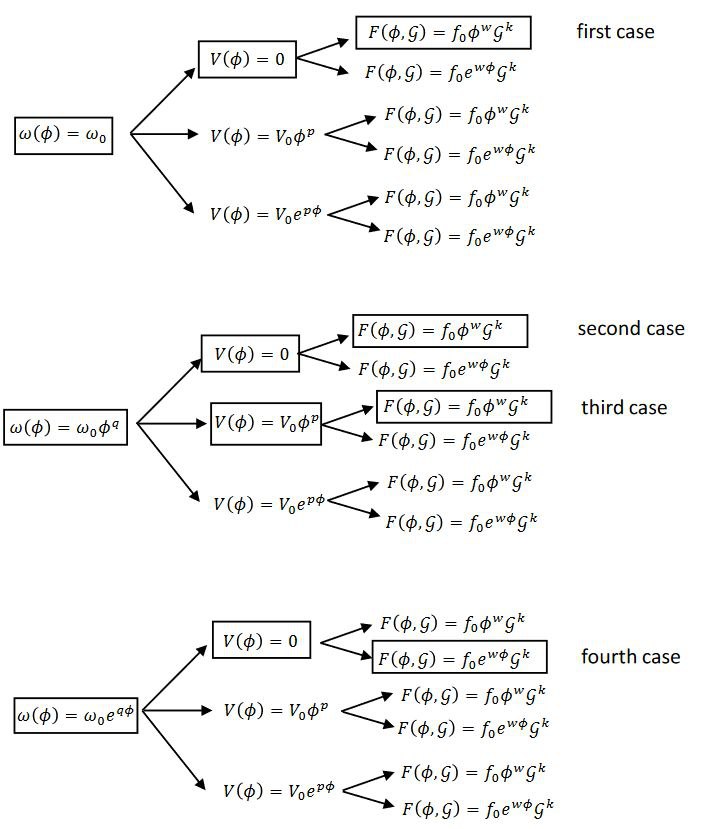
Figure 1: Possible forms of the Lagrangian function selected by the existence of symmetries.

For cosmological purposes, here we focus on the most interesting cases, which in Fig. 1 are marked by a rectangle, since they are the only symmetries leading either to time power-law or exponential de Sitter-like solutions. The other symmetries yield more complicated cosmological solutions, or equations of motions not solvable analytically. Though the latter category is still worth to be analysed, the study of numeric solutions is not the main goal of this paper. In the next subsections we analyse each case and find the corresponding cosmological solutions to the Euler–Lagrange equations.

III.1 First case

The first symmetry of the Lagrangian (34) occurs by setting $\omega(\phi)\sim\omega_{0}$ and $V(\phi)=0$, with $\omega_{0}$ being constant. In this case, the point-like Lagrangian reduces to:

$$\mathcal{L}=a^{3}\omega_{0}\dot{\phi}^{2}-f_{0}(k-1)\mathcal{G}^{k}\phi^{w}a^{3}-8f_{0}k\dot{a}^{3}\mathcal{G}^{k-2}\phi^{w-1}[(k-1)\phi\dot{\mathcal{G}}+w\mathcal{G}\dot{\phi}].$$ (37)

with infinitesimal symmetry generators of the form

$$\begin{split}&\alpha(a)=\alpha_{0}a,\hskip 8.5359pt\beta(\mathcal{G})=-4\xi_{0}\mathcal{G},\hskip 8.5359pt\gamma(\phi)=\dfrac{6(1-2k)\alpha_{0}}{-2+8k-w}\phi,\hskip 8.5359pt\xi(t)=-\dfrac{3(w-2)\alpha_{0}}{-2+8k-w}t,\end{split}$$ (38)

where $\alpha(a),\beta(\mathcal{G}),\gamma(\phi)$ and $\xi(t)$ are the infinitesimal generators of the coordinate transformations. Notice that, in agreement with Eq. (19j), the infinitesimal generator $\xi$ is a function of the sole time. In order to find analytic solutions to the equations of motion related to the Lagrangian (37), we can set $w=2$, so that the coupling function becomes $F(\phi,\mathcal{G})=f_{0}\phi^{2}\mathcal{G}^{k}$, meaning that the general gravitational action is:

$$S=\int\sqrt{-g}\left[f_{0}\phi^{2}\mathcal{G}^{k}+\omega_{0}\partial^{\mu}\phi\partial_{\mu}\phi\right]d^{4}x.$$ (39)

By these ansatz, the explicit forms of the scale factor and the scalar field are

$$a(t)=a_{0}e^{mt},\hskip 8.5359pt\phi(t)=\phi_{0}e^{nt},\hskip 8.5359pt\mathcal{G}=24m^{4},$$ (40)

namely de Sitter-like solutions. Here $a_{0},m,\phi_{0},n$ are real constants. A further constraint arising from the solution of the Euler–Lagrange equations concerns the relation among $\omega_{0},f_{0},n$ and $m$. Specifically, these four constants must satisfy the following system of algebraic equations:

$$\begin{cases}f_{0}(24m^{4})^{k}[3(k-1)m^{2}-4kmn-4kn^{2}]-3m^{2}n^{2}\omega_{0}=0\\ f_{0}(24m^{4})^{k}-n\omega_{0}(3m+n)=0\\ f_{0}(24m^{4})^{k}[(k-1)m-2kn]+mn^{2}\omega_{0}=0.\end{cases}$$ (41)

Solving the third equation with respect to $n$, we obtain two solutions. After choosing one, we can solve the energy equation with respect to the constant $f_{0}$ to obtain two other solutions. As a result, we have a total of four possible combinations, but only three of these are valid. For example, let us consider the cases $k=1$ and $k=1/2$; in particular, the latter is the value of $k$ allowing to recover GR at cosmological scales Bajardi:2020osh . For these two values, we get the solutions:

$$k=1/2,\hskip 28.45274ptn=-\dfrac{3}{2}m,\hskip 28.45274ptf_{0}=-\dfrac{3\sqrt{6}}{16}\omega_{0},$$ (42)

$$k=1,\hskip 28.45274ptn=-\dfrac{5}{2}m,\hskip 28.45274ptf_{0}=-\dfrac{5\omega_{0}}{96m^{2}}.$$ (43)

III.2 Second case

Another symmetry leading to exact cosmological solutions occurs once considering a vanishing potential, a power-law form of the kinetic term $\omega(\phi)$, i.e. $\omega(\phi)=\omega_{0}\phi^{q}$, and a coupling function of the form $F(\phi,\mathcal{G})=f_{0}\phi^{w}\mathcal{G}^{k}$. The Lagrangian thus reads:

$$\mathcal{L}=a^{3}[\omega_{0}\phi^{q}\dot{\phi}^{2}-f_{0}(k-1)\mathcal{G}^{k}\phi^{w}]-8f_{0}k\dot{a}^{3}\mathcal{G}^{k-2}\phi^{w-1}[(k-1)\phi\dot{\mathcal{G}}+w\mathcal{G}\dot{\phi}].$$ (44)

The existence of the Noether symmetry selects the following infinitesimal generators:

$$\alpha(a)=\alpha_{0}a,\hskip 8.5359pt\beta(\mathcal{G})=-4\xi_{0}\mathcal{G},\hskip 8.5359pt\gamma(\phi)=\dfrac{6(1-2k)\alpha_{0}}{(2+q)(4k-1)-w}\phi,\hskip 8.5359pt\xi(t)=-\dfrac{3(2+q-w)\alpha_{0}}{(2+q)(4k-1)-w}t,$$ (45)

and, as before, the infinitesimal generator $\xi$ is a function of the sole time. The system of Euler-Lagrange equations, together with the energy conditions, can be solved by setting $w=2+q$ and provides the following exponential solution:

$$a(t)=a_{0}e^{mt},\hskip 8.5359pt\phi(t)=\phi_{0}e^{nt},\hskip 8.5359pt\mathcal{G}=24m^{4}$$ (46)

where $n$ and $m$ are real constants. Due to the constraint imposed by the equations of motion, the infinitesimal generators become

$$\alpha(a)=\alpha_{0}a,\hskip 8.5359pt\beta(\mathcal{G})=0,\hskip 8.5359pt\gamma(\phi)=-\dfrac{3\alpha_{0}}{q+2}\phi,\hskip 8.5359pt\xi(t)=0$$ (47)

and the modified scalar-tensor action results

$$S=\int\sqrt{-g}\left[f_{0}\phi^{q+2}\mathcal{G}^{k}+\omega_{0}\phi^{q}\partial_{\mu}\phi\partial^{\mu}\phi\right]d^{4}x.$$ (48)

Also here, there is a further constraint coming from the equations of motion which sets the relation among the constants $f_{0},\omega_{0},m,n$, namely:

$$\begin{cases}f_{0}(24m^{4})^{k}[3(k-1)m^{2}-2kmn(q+2)-kn^{2}(q+2)^{2}]-3m^{2}n^{2}\omega_{0}=0\\ n\omega_{0}[6m+n(q+2)]-f_{0}(q+2)(24m^{4})^{k}=0\\ f_{0}(24m^{4})^{k}[(k-1)m-kn(q+2)]+mn^{2}\omega_{0}=0.\end{cases}$$ (49)

As the previous case, the solution of the above system results in four possible combinations for $f_{0}$ and $n$, but again only three are cosmologically meaningful. Considering the same values of $k$ as before, we obtain:

$$k=1/2,\hskip 28.45274ptn=-\dfrac{3}{q+2}m,\hskip 28.45274ptf_{0}=-\dfrac{3\sqrt{6}}{4(q+2)^{2}}\omega_{0},$$ (50)

$$k=1,\hskip 28.45274ptn=-\dfrac{5}{2+q}m,\hskip 28.45274ptf_{0}=-\dfrac{5\omega_{0}}{24(q+2)^{2}m^{2}}.$$ (51)

III.3 Third case

The third symmetry arising from the solution of the Noether system involves both the coupling function, the kinetic and the potential terms. Specifically, the Noether system can be solve if $\omega(\phi)=\omega_{0}\phi^{q}$, $V(\phi)=V_{0}\phi^{p}$ and $F(\phi,\mathcal{G})=f_{0}\phi^{w}\mathcal{G}^{k}$, with

$$q=\dfrac{w-4k+p(2k-1)}{2k}.$$ (52)

The Lagrangian (34) thus becomes:

$$\mathcal{L}=a^{3}[\omega_{0}\phi^{q}\dot{\phi}^{2}-f_{0}(k-1)\mathcal{G}^{k}\phi^{w}]-8f_{0}k\dot{a}^{3}\mathcal{G}^{k-2}\phi^{w-1}[(k-1)\phi\dot{\mathcal{G}}+w\mathcal{G}\dot{\phi}]+a^{3}V_{0}\phi^{p}$$ (53)

and it satisfies the existence condition of Noether symmetry provided that the infinitesimal generators take the form

$$\begin{split}&\alpha(a)=-\dfrac{1}{3}[\xi_{0}+kp\gamma_{0}]a,\hskip 8.5359pt\beta(\mathcal{G})=-4\xi_{0}\mathcal{G},\hskip 8.5359pt\gamma(\phi)=\gamma_{0}\phi,\hskip 8.5359pt\xi(t)=-\dfrac{(p-w)\gamma_{0}}{4k}t.\end{split}$$ (54)

A possible solution to the field equations consists of exponential scale factor and scalar field of the form:

$$a(t)=a_{0}e^{mt},\hskip 8.5359pt\phi(t)=\phi_{0}e^{nt},\hskip 8.5359pt\mathcal{G}=24m^{4},$$ (55)

with additional constraints given by the following system of algebraic equations:

$$\begin{cases}f_{0}(24m^{4})^{k}[kn^{2}w^{2}+2kmnw-3m^{2}(k-1)]+3m^{2}n^{2}\omega_{0}+3m^{2}V_{0}=0\\ w=q+2\\ p=w\\ f_{0}(24m^{4})^{k}w-n\omega_{0}(6m+n(q+2))+pV_{0}=0\\ f_{0}(24m^{4})^{k}[knw-m(k-1)]-mn^{2}\omega_{0}+mV_{0}=0\,.\\ \end{cases}$$ (56)

By replacing the second and the third equation into Eq. (54), the latter becomes:

$$\begin{split}&\alpha(a)=-\dfrac{kw\gamma_{0}}{3}a,\hskip 8.5359pt\beta(\mathcal{G})=0,\hskip 8.5359pt\gamma(\phi)=\gamma_{0}\phi,\hskip 8.5359pt\xi(t)=0.\end{split}$$ (57)

According to the discussion in Sec. II, the generators of Eq. (57) describe an internal symmetry, due to the condition $\xi(t)=0$. Therefore, symmetries corresponding to this third case can be also selected by the vanishing Lie derivative condition. Unlike the other cases, here the system (56) yields different solutions, but only one of these is completely real. The other solutions, in fact, contain at least one imaginary parameter and have been excluded for obvious physical reasons. For $k=1$ and $k=1/2$, the solution takes the form:

$$k=1/2,\hskip 28.45274ptn=-\dfrac{3w}{2\omega_{0}}m+\dfrac{\sqrt{m}}{2\omega_{0}}\dfrac{3w^{2}-4w\omega_{0}}{\sqrt{(w^{4}+4\omega_{0}^{2})^{2}-4w^{2}\omega_{0}}},\hskip 28.45274ptf_{0}=-\dfrac{\sqrt{6}}{2},$$ (58)

$$k=1,\hskip 28.45274ptn=-\dfrac{6\sqrt{6}w}{\omega_{0}}m^{3}-\dfrac{4\sqrt{6}w}{\omega_{0}}m^{3}\biggl{(}\dfrac{3\sqrt{6}m^{2}w^{2}-\omega_{0}}{2\sqrt{6}m^{2}w^{2}-\omega_{0}}\biggr{)},\hskip 28.45274ptf_{0}=-\dfrac{\sqrt{6}}{2}.$$ (59)

III.4 Fourth case

Let us finally analyse the last symmetry selected by the approach, consisting of an exponential kinetic term (i.e. $\omega(\phi)=\omega_{0}e^{q\phi}$), a vanishing potential and a coupling function of the form $F(\phi,\mathcal{G})=f_{0}e^{w\phi}\mathcal{G}^{\frac{1}{2}}$. The corresponding Lagrangian is

$$\mathcal{L}=2\mathcal{G}^{-\frac{3}{2}}f_{0}\dot{a}^{3}e^{w\phi}\left(\dot{\mathcal{G}}-2w\mathcal{G}\dot{\phi}\right)+a^{3}\left(\dfrac{1}{2}f_{0}\mathcal{G}^{\frac{1}{2}}e^{w\phi}+\omega_{0}e^{q\phi}\dot{\phi}^{2}\right).$$ (60)

It is interesting to notice that here the power of $\mathcal{G}$ selected by the Noether Symmetry Approach is not a general constant as the previous cases, but the only coupling function containing symmetries set the value of $k$ to $1/2$. This means that the equivalence with GR in cosmological backgrounds (since $R^{2}\sim\mathcal{G}$ in FRW cosmology) naturally arises from symmetry considerations and has not to be imposed as a requirement. The Noether symmetry existence condition also selects the following infinitesimal generators:

$$\begin{split}&\alpha(a)=-\dfrac{\beta_{0}}{12}a,\hskip 8.5359pt\beta(\mathcal{G})=\beta_{0}\mathcal{G},\hskip 8.5359pt\gamma(\phi)=0,\hskip 8.5359pt\xi(t)=-\dfrac{\beta_{0}}{4}t,\\ \end{split}$$ (61)

where, also here, $\xi$ is a function of time. A possible solutions to the equations of motion is given by:

$$a(t)=a_{0}e^{mt},\hskip 8.5359pt\phi(t)=\phi_{0}t,$$ (62)

with $m,a_{0},\phi_{0}$ being integration constants. In addition, from the Euler-Lagrange equations, we get three constraints on the free parameters, resulting in the following system:

$$\begin{cases}2f_{0}m^{2}(3m^{2}+2mw\phi_{0}+w^{2}\phi_{0}^{2})+\sqrt{6}m^{2}\omega_{0}\phi_{0}^{2}=0\\ w=q\\ 2\sqrt{6}f_{0}m^{2}w-\omega_{0}\phi_{0}(6m+w\phi_{0})=0\\ \sqrt{6}m^{2}\omega_{0}\phi_{0}^{2}-6f_{0}m^{3}(m+w\phi_{0})=0.\end{cases}$$ (63)

To solve the above system, we find $f_{0}$ from the third equation and then we solve the energy condition with respect to $\phi_{0}$, so that we get two different solutions, namely:

$$\phi_{0}=-\dfrac{3m}{w},\hskip 28.45274ptf_{0}=-\biggl{(}\dfrac{3}{2}\biggr{)}^{\frac{3}{2}}\dfrac{\omega_{0}}{w^{2}},$$ (64)

$$\phi_{0}=-\dfrac{2m}{w},\hskip 28.45274ptf_{0}=-2\sqrt{\dfrac{2}{3}}\dfrac{\omega_{0}}{w^{2}}.$$ (65)

The above solutions can be further simplified by choosing $f_{0}=\sqrt{6}/2$. In this way we get:

$$\phi_{0}=-\dfrac{3m}{w},\hskip 28.45274ptf_{0}=\frac{\sqrt{6}}{2},\hskip 28.45274pt\omega_{0}=\frac{2}{3}w^{2},$$ (66)

$$\phi_{0}=-\dfrac{2m}{w},\hskip 28.45274ptf_{0}=\frac{\sqrt{6}}{2},\hskip 28.45274pt\omega_{0}=\frac{4}{3}w^{2}.$$ (67)

IV Conclusion

We outlined the main properties of the Noether Symmetry Approach discussing some applications and showing how to use the Noether theorem as a method to select theories containing symmetries. Starting from canonical Lagrangians, we first introduced the prescriptions aimed at constraining the generator of the symmetry. This approach is particularly useful in modified theories of gravity Bajardi:2022ypn , or in quantum cosmology, where the conserved quantity allows to restrict the variables superspace to integrable minisuperspaces Lambiase ; Capozziello:2022vyd . The first prolongation of the Noether vector yields a more general class of symmetries, which reduce to those coming from the application of vanishing Lie derivative when the functions determining prolongations are $g=const$ and $\xi=0$. Moreover, an important result arises from the application of Noether symmetry approach to canonical Lagrangians: the infinitesimal generator $\xi$ related to spacetime translations turns out to be a function of the sole time. This result permits to further simplify the approach by reducing the system of differential equations.

This feature becomes evident when applying the prescription to modified theories of gravity; specifically, in the second part of the manuscript, we focused on a modified gravitational action containing both the Gauss-Bonnet topological term and a dynamical scalar field. The selection of viable models has been pursued by searching for symmetries. In other words, viable modified theories of gravity can be selected adopting a physical criterium based on symmetry considerations.

Each symmetry can be related to a conserved quantity that can thus be used to reduce dynamical equations. As output of the process, viable cosmological solutions are derived as power-law or de Sitter behaviors. In this perspective, the Noether Symmetry Approach results a method capable of selecting physically viable models.

References

• (1) C. W. Misner, K. S. Thorne and J. A. Wheeler, W. H. Freeman, 1973, ISBN 978-0-7167-0344-0, 978-0-691-17779-3
• (2) B. P. Abbott et al. [LIGO Scientific and Virgo], Phys. Rev. Lett. 116 (2016) no.6, 061102
• (3) K. Akiyama et al. [Event Horizon Telescope], Astrophys. J. Lett. 875 (2019), L1
• (4) K. Akiyama et al. [Event Horizon Telescope], Astrophys. J. Lett. 875 (2019) no.1, L5
• (5) C. M. Will, Living Rev. Rel. 17 (2014), 4
• (6) S. Nojiri, S. D. Odintsov and V. K. Oikonomou, Phys. Rept. 692 (2017), 1-104
• (7) S. D. Odintsov, V. K. Oikonomou, I. Giannakoudi, F. P. Fronimos and E. C. Lymperiadou, [arXiv:2307.16308 [gr-qc]].
• (8) J. Beringer et al. [Particle Data Group], Phys. Rev. D 86 (2012), 010001
• (9) A. Bosma, Astron. J. 86 (1981), 1825
• (10) J. Frieman, M. Turner and D. Huterer, Ann. Rev. Astron. Astrophys. 46 (2008), 385-432
• (11) A. G. Riess et al. [Supernova Search Team], Astron. J. 116 (1998), 1009-1038
• (12) T. Vachaspati, D. Stojkovic and L. M. Krauss, Phys. Rev. D 76 (2007), 024005
• (13) C. Barceló, S. Liberati, S. Sonego and M. Visser, Sci. Am. 301 (2009) no.4, 38-45
• (14) M. H. Goroff and A. Sagnotti, Nucl. Phys. B 266 (1986), 709-736
• (15) N. D. Birrell and P. C. W. Davies, Cambridge Univ. Press, 1984, ISBN 978-0-521-27858-4, 978-0-521-27858-4
• (16) S. Weinberg, Rev. Mod. Phys. 61 (1989), 1-23
• (17) M. Niedermaier and M. Reuter, Living Rev. Rel. 9 (2006), 5-173
• (18) R. Percacci, [arXiv:0709.3851 [hep-th]].
• (19) F. Bajardi, F. Bascone and S. Capozziello, Universe 7 (2021) no.5, 148
• (20) S. Alexandrov and E. R. Livine, Phys. Rev. D 67 (2003), 044009
• (21) J. M. Maldacena, Adv. Theor. Math. Phys. 2 (1998), 231-252
• (22) H. P. Nilles, Phys. Rept. 110 (1984), 1-162
• (23) C. Rovelli, Living Rev. Rel. 1 (1998), 1
• (24) P. Horava, Phys. Rev. D 79 (2009), 084008
• (25) V. A. Rubakov and M. E. Shaposhnikov, Phys. Lett. B 125 (1983), 136-138
• (26) F. Bajardi, D. Vernieri and S. Capozziello, JCAP 11 (2021) no.11, 057
• (27) L. e. Qiang, Y. Gong, Y. Ma and X. Chen, Phys. Lett. B 681 (2009), 210-213
• (28) S. M. M. Rasouli, S. Jalalzadeh and P. Moniz, Universe 8 (2022) no.8, 431
• (29) F. Bajardi and S. Capozziello, “Noether Symmetries in Theories of Gravity,” Cambridge University Press, Cambridge 2022,
ISBN 978-1-00-920872-7, 978-1-00-920874-1
• (30) S. Capozziello and M. De Laurentis, Phys. Rept. 509 (2011), 167-321
• (31) T. P. Sotiriou and V. Faraoni, Rev. Mod. Phys. 82 (2010), 451-497
• (32) A. K. Mishra, M. Rahman and S. Sarkar, Class. Quant. Grav. 35 (2018) no.14, 145011
• (33) J. L. Blázquez-Salcedo, F. S. Khoo and J. Kunz, Phys. Rev. D 96 (2017) no.6, 064008
• (34) K. S. Stelle, Phys. Rev. D 16 (1977), 953-969
• (35) J. J. Halliwell, Phys. Lett. B 185 (1987), 341
• (36) J. P. Uzan, Phys. Rev. D 59 (1999), 123510
• (37) S. Capozziello, Int. J. Mod. Phys. D 11 (2002), 483-492
• (38) B. Cvetković and D. Simić, Phys. Rev. D 94 (2016) no.8, 084037
• (39) J. Zanelli, [arXiv:hep-th/0502193 [hep-th]].
• (40) D. Comelli, Phys. Rev. D 72 (2005), 064018
• (41) F. Bajardi and R. D’Agostino, Gen. Rel. Grav. 55 (2023) no.3, 49
• (42) S. Capozziello, R. De Ritis, C. Rubano and P. Scudellaro, Riv. Nuovo Cim. 19N4 (1996), 1-114
• (43) F. Bajardi and S. Capozziello, Eur. Phys. J. C 80 (2020) no.8, 704
• (44) K. F. Dialektopoulos and S. Capozziello, Int. J. Geom. Meth. Mod. Phys. 15 (2018) no.supp01, 1840007
• (45) Z. Urban, F. Bajardi and S. Capozziello, Int. J. Geom. Meth. Mod. Phys. 17 (2020) no.14, 2050215
• (46) S. Capozziello, A. Stabile and A. Troisi, Class. Quant. Grav. 24 (2007), 2153-2166
• (47) S. Capozziello and G. Lambiase, Gen. Rel. Grav. 32 (2000), 295-311
• (48) S. Basilakos, M. Tsamparlis and A. Paliathanasis, Phys. Rev. D 83 (2011), 103512
• (49) S. Capozziello, G. Marmo, C. Rubano and P. Scudellaro, Int. J. Mod. Phys. D 6 (1997), 491-503
• (50) S. Capozziello, M. De Laurentis and S. D. Odintsov, Eur. Phys. J. C 72 (2012), 2068
• (51) F. Bajardi and S. Capozziello, Eur. Phys. J. C 83 (2023) no.6, 531
• (52) S. Capozziello and F. Bajardi, Universe 8 (2022) no.3, 177
• (53) S. Bahamonde and S. Capozziello, Eur. Phys. J. C 77 (2017) no.2, 107
• (54) F. Bajardi, K. F. Dialektopoulos and S. Capozziello, Symmetry 12 (2020) no.3, 372
• (55) S. Bahamonde, K. Dialektopoulos and U. Camci, Symmetry 12 (2020) no.1, 68
• (56) S. Bahamonde and U. Camci, Symmetry 11 (2019) no.12, 1462
• (57) P. Agrawal, S. Gukov, G. Obied and C. Vafa, [arXiv:2009.10077 [hep-th]].
• (58) S. Capozziello and G. Lambiase, Gen. Rel. Grav. 32 (2000), 673-696