The dynamical induced quark spin polarization by magnetic field at the early stage of heavy-ion collisions

Abstract

We present a comprehensive analysis of the dynamic process of quark spin polarization induced by magnetic fields at the pre-thermal stage in heavy-ion collisions by using the recently developed theoretical tool of chiral kinetic theory. Our findings demonstrate that the spin polarization of quarks is highly sensitive to the interactions between quarks. These interactions can delay the decay of early spin polarization vector while accelerating the decay of later spin polarization vector. Specifically, our simulations show the detailed process of how magnetic fields polarize quarks within the fireball and reveal that quark interactions lead to an acceleration effect on the average spin. Notably, the fireball in the early stage has an incomplete electromagnetic response effect, there is a delayed effect on the increase of the induced magnetic field.

I Introduction

The spin degree of freedom is a fundamental characteristic of modern physics that has numerous applications in various fields. In particular, in heavy-ion collisions, it has been attracted considerable attention to studying many physical phenomena related to spin, especially the quark matter under external magnetic field and vortical field, such as the chiral magnetic effect  Kharzeev:2004ey ; Kharzeev:2007tn ; Kharzeev:2007jp ; Fukushima:2008xe , chiral magnetic wave Kharzeev:2010gd ; Burnier:2011bf , Chiral vortical effects Son:2009tf ; Kharzeev:2010gr ; Sadofyev:2010is ; Landsteiner:2011iq ; Jiang:2015cva , and spin polarization effect STAR:2017ckg ; STAR:2018gyt ; STAR:2019erd ; Niida:2018hfw ; ALICE:2019onw , etc.

The spin polarization of $\Lambda$ and $\bar{\Lambda}$ hyperons have been observed in 7.7- 200 A GeV Au + Au collisions through the angular distribution of their weak-decay products STAR:2017ckg ; STAR:2018gyt ; STAR:2019erd ; Niida:2018hfw . The global spin polarization effect has been successfully described by the thermal vorticity effects Becattini:2013fla ; Fang:2016vpj ; Pang:2016igs . Recently, the “spin sign puzzle” Liu:2019krs ; Wu:2019eyi ; Florkowski:2019voj of the local $\Lambda$ polarization also has been explained by the shear-induced polarization (SIP) effect Fu:2021pok ; Fu:2020oxj . Despite extensive research, the splitting of polarization between $\Lambda$ and $\bar{\Lambda}$ hyperons remains an open question Muller:2018ibh ; Guo:2019mgh ; Guo:2019joy ; Han:2019fce ; Becattini:2020ngo ; Xu:2022hql . Recently, the strong magnetic fields present in heavy-ion collisions have been proposed to understand the polarization splitting puzzle in $\Lambda$ and $\bar{\Lambda}$ hyperons Xu:2022hql .

There has been significant interest in recent years in studying the spin polarization of hyperons in heavy-ion collisions. However, describing the detailed dynamic spin polarization of quarks in quark-gluon plasma fireballs remains a significant challenge. The spin polarization of $\Lambda$ hyperons in heavy-ion collisions is believed to be encoded in the behavior of quarks in quark-gluon plasma (QGP), particularly the strange quark Fu:2021pok ; Fu:2020oxj . Therefore, understanding the behavior of the strange quark in QGP is the key to unraveling the spin-splitting puzzle in $\Lambda$ hyperons. At present, the quantitative modeling of spin polarization of $\Lambda$ hyperons is quantitatively modeled only at the freeze-out surface of hydrodynamics using the spin Cooper-Frye formula. However, an unresolved crucial issue is the detailed evolution of the spin polarization of quarks in QGP.

In this study, we take an important step towards addressing this challenge by using the recently developed theoretical tool of chiral kinetic theory Stephanov:2012ki ; Son:2012wh ; Son:2012zy ; Chen:2012ca ; Kharzeev:2016sut ; Chen:2012ca ; Hidaka:2016yjf ; Mueller:2017arw ; Gorbar:2017cwv ; Huang:2018wdl to investigate the dynamic evolution of the spin splitting between quarks and anti-quarks induced by magnetic field at the pre-thermal stage of heavy-ion collisions. At this stage, the quark-gluon plasma is far from thermal equilibrium and the magnetic field is at its strongest. In the chiral limit, the properties of the d and s quarks are identical, including their charge. As a result, for our simulation, we will only need to consider the u and d quarks.

The paper is organized as following: after introduction, we will introduce the theoretical framework in Sec.II, and we present numerical method and results in Sec.III and Sec.IV, and we give a summary in Sec. V.

II The theoretical framework

The theoretical framework to describe the transport phenomenon of chiral quarks under electromagnetic fields in an out-of-equilibrium system is composed of the chiral kinetic theory and Maxwell equations Stephanov:2012ki ; Son:2012wh ; Son:2012zy ; Chen:2012ca ; Kharzeev:2016sut ; Chen:2012ca ; Hidaka:2016yjf ; Mueller:2017arw ; Gorbar:2017cwv ; Huang:2018wdl . The chiral kinetic equation is to take the following form Huang:2018wdl :

$$\begin{split}&\Bigg{\{}\partial_{t}+\dot{\mathbf{x}}\cdot\triangledown_{\mathbf{x}}+\dot{\mathbf{p}}\cdot\triangledown_{\mathbf{p}}\Bigg{\}}f^{i}_{\chi}(x,\mathbf{p})=C[f^{i}_{\chi}].\end{split}$$ (1)

with

$$\begin{split}&\dot{\mathbf{x}}=\frac{1}{\sqrt{G}}\left(\widetilde{\boldsymbol{v}}+\hbar q_{i}(\widetilde{\boldsymbol{v}}\cdot\mathbf{b}_{\chi})\mathbf{B}+\hbar q_{i}\widetilde{\mathbf{E}}\times\mathbf{b}_{\chi}\right),\\ &\dot{\mathbf{p}}=\frac{q_{i}}{\sqrt{G}}\left(\widetilde{\mathbf{E}}+\widetilde{\boldsymbol{v}}\times\mathbf{B}+\hbar q_{i}(\widetilde{\mathbf{E}}\cdot\mathbf{B})\mathbf{b}_{\chi}\right).\end{split}$$ (2)

Where the corresponding Jacobian, energy, group velocity are

$$\sqrt{G}=\left(1+\hbar q_{i}\mathbf{b}_{\chi}\cdot\mathbf{B}\right),$$

$$\widetilde{\mathbf{E}}=\mathbf{E}-\frac{1}{q_{i}}\triangledown_{\mathbf{x}}E_{\mathbf{p}},~{}~{}~{}E_{\mathbf{p}}=|\mathbf{p}|\left(1-\hbar q_{i}\mathbf{B}\cdot\bf{b}_{\chi}\right),$$

$$\widetilde{\boldsymbol{v}}=\frac{\partial E_{\mathbf{p}}}{\partial\mathbf{p}}=\widehat{\mathbf{p}}\left(1+2\hbar q_{i}\mathbf{B}\cdot\mathbf{b}_{\chi}\right)-\hbar q_{i}b_{\chi}\mathbf{B}.$$

Where $q_{i}$ is the electric charge of the chiral fermion, $\chi$ the chirality, and $\mathbf{b}_{\chi}=\chi\frac{\mathbf{p}}{2|\mathbf{p}|^{3}}$ the Berry curvature. While $f^{i}_{\chi}$ is the distribution function in the phase space of position $\bf x$ and momentum $\bf p$ for each specie (labelled by $i$) of chiral fermions, and $C[f^{i}_{\chi}]$ is the collision term.

The companied Maxwell equations can be written as the following,

$$\begin{split}&\triangledown\cdot\mathbf{E}=\rho_{e},\\ &\triangledown\cdot\mathbf{B}=0,\\ &\partial_{t}\mathbf{E}=\triangledown\times\mathbf{B}-\mathbf{j}_{e},\\ &\partial_{t}\mathbf{B}=-\triangledown\times\mathbf{E}.\end{split}$$ (3)

Where $\rho_{e}$ and $\mathbf{j}_{e}$ are the charge and charge current density, respectively. In heavy-ion collisions, they can be divided into two parts as $\rho_{e}=\rho^{\text{ext}}_{e}+\rho^{\text{int}}_{e}$ and $\mathbf{j}_{e}=\mathbf{j}^{ext}_{e}+\mathbf{j}^{int}_{e}$ mclerran2014comments ; Huang:2022qdn . Herein, $\rho^{\text{ext}}_{e}$ and $\mathbf{j}^{ext}_{e}$ are the contribution coming from an external source like the fast-moving charged particles, which are the protons from colliding nuclei. While $\rho^{\text{int}}_{e}$ and $\mathbf{j}^{int}_{e}$ are contributions from the medium, which can be derived by the chiral distribution function as following,

$$\begin{split}&\rho^{int}_{e}=\sum_{i}q_{i}\sum_{\chi=\pm}\int\frac{d^{3}p}{(2\pi)^{3}}\sqrt{G}f^{i}_{\chi}(x,\mathbf{p}),\\ &\mathbf{j}^{int}_{e}=\sum_{i}q_{i}\sum_{\chi=\pm}\int\frac{d^{3}p}{(2\pi)^{3}}\sqrt{G}\dot{\mathbf{x}}f^{i}_{\chi}(x,\mathbf{p}).\end{split}$$ (4)

Herein the species $i=(u,\bar{u},d,\bar{d})$, with the electric charge $q_{u}=-q_{\bar{u}}=\frac{2e}{3}$ and $q_{d}=-q_{\bar{d}}=-\frac{e}{3}$. It is explicit that the internal electric density and current density are the bridge between the chiral transport equations and Maxwell’s equations.

In this work, we will focus on the dynamical spin polarization of the quarks $\mathbf{P}_{i}$ in QGP, which can be quantified by the axial current scaled by the number of the quark Liu:2019krs ,

$$\begin{split}&\mathbf{P}_{i}(t)=\frac{\int d^{3}x\,\mathbf{j}_{5,i}(t,\mathbf{x})}{\int d^{3}x\,n_{i}(t,\mathbf{x})}\\ &~{}~{}~{}~{}~{}~{}~{}~{}=\frac{\int d^{3}x\left(\mathbf{j}_{i,R}(t,\mathbf{x})-\mathbf{j}_{i,L}(t,\mathbf{x})\right)}{\int d^{3}x\left(n_{i,R}(t,\mathbf{x})+n_{i,L}(t,\mathbf{x})\right)}\\ &~{}~{}~{}~{}~{}~{}~{}~{}=\frac{\mathbf{J}_{i,R}(t)-\mathbf{J}_{i,L}(t)}{N_{i,R}+N_{i,L}}.\end{split}$$ (5)

The number and chiral current of quarks are expressed by the following,

$$\begin{split}N_{i,\chi}(t)&=\int\frac{d^{3}pd^{3}x}{(2\pi)^{3}}\sqrt{G}f^{i}_{\chi}(x,\mathbf{p}),\\ \mathbf{J}_{i,\chi}(t)&=\int d^{3}x\mathbf{j}_{i,\chi}(t,\mathbf{x})\\ &=\int\frac{d^{3}pd^{3}x}{(2\pi)^{3}}\sqrt{G}\dot{\mathbf{x}}f^{i}_{\chi}(x,\mathbf{p}).\end{split}$$ (6)

Where $\chi=\pm$ or $\chi=R/L$ denotes the right/left-hand quark. While another vital quantity to describe the dynamical evolution of spin polarization of quarks is the average spin vector, defined as the following,

$$\mathbf{S}_{i}(t) =\int d^{3}x\mathbf{S}_{i}(t,\mathbf{x})$$

$$=\sum_{\chi=\pm}\frac{1}{N_{i}}\int\frac{d^{3}pd^{3}x}{(2\pi)^{3}}\frac{\chi}{2}\hat{\mathbf{p}}f^{i}_{\chi}(x,\mathbf{p}).$$ (7)

Where $N_{i}=N_{i,R}+N_{i,L}$ is the total number of species $i$ particle, and herein $\mathbf{S}_{i}(t,\mathbf{x})$ the average spin density vector. In fact, by comparing this equation with Eq.(5), it is clear that $2\mathbf{S}_{i}(t)$ is the zeroth order part of the spin polarization defined in Eq.(5), which can be seen by combining Eq.(2) and Eq.(6) into the Eq.(5).

III The Strategy for numerical calculation

To consistently solve the chiral transport equation Eq.(1) and Maxwell’s equations Eq.(3), we choose split method to solve the chiral transport equationaristov2001direct , and select the Yee-grid algorithm to solve Maxwell’s equationyee1966numerical ; mclerran2014comments ; Huang:2022qdn .

We show the detailed algorithm for the simulation. Firstly, the chiral transport equation Eq.(1) is divided into the free-streaming transport equation and collision equation in a time interval $[t,t+dt]$ like the following

$$\begin{split}&\Bigg{\{}\partial_{t}+\dot{\mathbf{x}}\cdot\triangledown_{\mathbf{x}}+\dot{\mathbf{p}}\cdot\triangledown_{\mathbf{p}}\Bigg{\}}f^{i}_{1\chi}(x,\mathbf{p})=0.\\ &f^{i}_{1\chi}(t)=f^{i}_{\chi}(t).\\ &\partial_{t}f^{i}_{2\chi}(x,\mathbf{p})=C[f^{i}_{2\chi}],\\ &f^{i}_{2\chi}(t)=f^{i}_{1\chi}(t+dt).\end{split}$$ (8)

Herein, the distribution function at time $t$ is the initial condition of the free transport equation, the solution of the free-streaming transport equation at next time $t+dt$ is the initial condition of the collision equation. The solution of the collision equation at $t+dt$ is the physical distribution function at $t+dt$, i.e. $f^{i}_{\chi}(t+dt)=f^{i}_{2\chi}(t+dt)$. This method is now widely used to simulate the transport equation. For the free transport equation, one can choose different numerical methods to further calculate, such as the finite difference method, finite volume method, and test particle methodbird1994molecular ; grigoryev2012numerical ; aristov2001direct . In this work, we take the finite difference method.

For Maxwell’s equations we will firstly take the split method used by McLerran and SkokovMcLerran:2013hla to separate Maxwell equations into the external part and internal part before further numerical calculation. In which, the electric and magnetic fields are separated into two pieces, i.e

$$\mathbf{E}=\mathbf{E}_{ext}+\mathbf{E}_{int},~{}~{}~{}\mathbf{B}=\mathbf{B}_{ext}+\mathbf{B}_{int}.$$ (9)

Herein, ”ext” denotes the external part which is originated by the source contribution, such as the fast moving charge particles in heavy-ion collisions, while the ”int” regards to the induced internal electromagnetic fields in the medium of quark-gluon plasma (QGP). The Maxwell equations in Eq.(3) now can been split into two parts. For the ”external” part,

$$\begin{split}&\triangledown\cdot\mathbf{E}_{ext}=\rho^{\text{ext}}_{e},\\ &\partial_{t}\mathbf{E}_{ext}=\triangledown\times\mathbf{B}_{ext}-\mathbf{J}^{\text{ext}}_{e},\\ &\triangledown\cdot\mathbf{B}_{ext}=0,\\ &\partial_{t}\mathbf{B}_{ext}=-\triangledown\times\mathbf{E}_{ext}.\end{split}$$ (10)

Herein, $\rho^{\text{ext}}_{e}$ and $\mathbf{J}^{\text{ext}}_{e}$ are the external source contributions, which are from the fast-moving charged particles, mainly the protons of colliding nuclei. They can be written as

$$\rho^{\text{ext}}_{e}=e\sum_{i}\delta(\mathbf{x}_{\perp}-\mathbf{x}^{{}^{\prime}}_{\perp,i})\delta(z-z^{{}^{\prime}}_{i}-\beta t),$$

$$\mathbf{J}^{\text{ext}}_{e}=e\sum_{i}\beta\hat{z}\,\delta(\mathbf{x}_{\perp}-\mathbf{x}^{{}^{\prime}}_{\perp,i})\delta(z-z^{{}^{\prime}}_{i}-\beta t).$$ (11)

Since the solutions are the electric and magnetic fields induced by the fast moving charged particles, the solutions of the set of equations (10) can be obtained by boosting the electric field of the protons both in projectile and target as Refmclerran2014comments ; Zakharov:2014dia ; Huang:2022qdn . The distribution of protons both in projectile and target can be modeled by the Woods-Saxon distribution with the standard parametersalver2008phobos . While the ”internal” part of Maxwell’s equation (3) is,

$$\begin{split}&\triangledown\cdot\mathbf{E}_{int}=\rho^{int}_{e},\\ &\partial_{t}\mathbf{E}_{int}=\triangledown\times\mathbf{B}_{int}-\mathbf{J}^{int}_{e},\\ &\triangledown\cdot\mathbf{B}_{int}=0,\\ &\partial_{t}\mathbf{B}_{int}=-\triangledown\times\mathbf{E}_{int}.\end{split}$$ (12)

Where the internal density $\rho^{int}_{e}$ and current density $\mathbf{J}^{int}_{e}$ are of the electric charge density and electric current density of the QGP, respectively, which are given by the following equations.

$$\begin{split}&\rho^{int}_{e}=\sum_{i}q_{i}\sum_{\chi=\pm}\int\frac{d^{3}p}{(2\pi)^{3}}\sqrt{G}f^{i}_{\chi}(x,\mathbf{p}),\\ &\mathbf{j}^{int}_{e}=\sum_{i}q_{i}\sum_{\chi=\pm}\int\frac{d^{3}p}{(2\pi)^{3}}\sqrt{G}\dot{\mathbf{x}}f^{i}_{\chi}(x,\mathbf{p}).\end{split}$$ (13)

We will select the Yee-grid algorithmYee:1966 to solve this set of equations to get the internally induced electric and magnetic fields.

With the above numerical method, we now apply it to study the spin polarization of quarks that are generated during the early moments in heavy ion collisions when the created QGP is still out-of-equilibrium while the magnetic field is the strongest. The created QGP at early time is characterized by the saturation scale $Q_{s}$, it is on the order of $1\sim 3\rm GeV$ for RHIC and the LHC Kowalski:2007rw . We will take $Q_{s}\simeq 2\rm GeV$ in this work. According to the works blaizot2012bose ; blaizot2013gluon ; blaizot2014quark , the physical picture of the early stage in heavy-ion collisions is that the system is initially gluon-dominated on the time interval $0\sim 1/Q_{s}$, the quarks are generated quickly on a time scale $t\sim 1/Q_{s}$ and then evolve toward thermal equilibrium. In this work, we take the formation time $t_{in}=0.1{\rm fm/c}$ as the starting time of the evolution of quarks and $t_{f}=0.6{\rm fm/c}$ the end of time which is on the order of onset time for hydrodynamic evolution in heavy ion collisions.

We take the same quark initial distributions $f_{0}$ at $t=t_{in}$ with the previous workHuang:2017tsq :

$$f_{0}=n_{0}\,{\cal F}\left(|\vec{\bf p}|\right)\,\exp\left[-\frac{x^{2}}{R_{x}^{2}}-\frac{y^{2}}{R_{y}^{2}}-\frac{z^{2}}{R_{z}^{2}}\right],$$ (14)

Here, there is no chirality imbalance, the number of right-handed and left-handed quarks is set to be the same. The spatial distribution is set to be Gaussian, with three width parameters, $R_{z}=1/(2Q_{s})$, $R_{x}\to(R_{A}-b/2)$ and $R_{y}\to\sqrt{R_{A}^{2}-(b/2)^{2}}$. Herein, the transverse widths ($R_{x},R_{y}$) are determined by the nuclear geometry with nuclear radius $R_{A}$ and the impact parameter $b$. We choose the Fermi-Dirac-like form to simulate the initial momentum distribution ${\cal F}$, i.e

$${\cal F}_{FD}=\frac{1}{e^{(p-Q_{s})/\Delta}+1},~{}~{}~{}\text{ with $\Delta=0.2\rm GeV$}$$ (15)

The overall parameter $n_{0}$ is fixed by normalizing the quark number density at the fireball center via $\int_{\vec{\bf p}}f_{0}(\vec{\bf p},x=y=z=0)\to\xi Q_{s}^{3}$ blaizot2014quark and the parameter $\xi$ will be varied in a reasonable range to be consistent with that of typical initial condition used for hydrodynamic simulations.

In this work, the collision term is chosen as the familiar relaxation time approximation (RTA) method for simplicity,

$$C[f^{i}]\approx-\frac{f^{i}-f^{i}_{eq}}{\tau_{R}}.$$ (16)

Where the local equilibrium distribution function $f_{eq}=1/(e^{(\epsilon-\mu)/T}+1)$ should be determined self-consistently at any space-time point during the evolution, herein the effective local equilibrium parameters $T(t,\mathbf{x})$ and $\mu(t,\mathbf{x})$ can be fixed by the matching conditions for the energy density and number density, i.e $e_{eq}=e$ and $n_{eq}=n$.

The induced electric and magnetic fields have been neglected when solving the distribution function by Eq.(8). This is also consistent with the previous worksVoronyuk:2011jd ; Zakharov:2014dia ; Wang:2021oqq , These works show us that the induced magnetic field is negligible compared to the external magnetic field at the early stage in heavy-ion collisions. Then when numerically solving the chiral transport equation Eq.(8), the contributions of the induced electric and magnetic fields will be ignored.

For the rest of the paper we will focus on the case of impact parameter $b=8.87\rm\,fm$ corresponding roughly to $20-50\%$ centrality class. One should notice that the external electric and magnetic fields are controlled by the impact parameter by fixing the center of the projectile and target on the coordinates $(-b/2,0,0)$ and $(b/2,0,0)$ respectively at the time $t=0\rm\,fm$. We use a spatial volume of $31\times 31\times 81\rm\,fm^{3}$ with grid size $(dx,dy,dz)=(0.8,0.8,0.035)$ fm and a finite time step $\Delta t=0.002\rm\,fm/c$ when we solve the kinetic equations Eq.(8) and Maxwell equations Eq.(12), while the momentum volume is set to be $26\times 26\times 26\rm\,fm^{-3}$ with grid size $(dp_{x},dp_{y},dp_{z})=(2,2,2)\rm\,fm^{-1}$. In our numerical simulations, the total number of quarks and the total energy are nearly conserved between the start time $0.1$fm and the end time $0.6$fm with a very small change.

IV Results and Discussions

Let us firstly demonstrate the out-of-equilibrium spin polarization of the quarks induced by the magnetic field by examining the transverse component $\vec{S}_{f}^{\perp}$ of the spin average density on the $x-y$ plane at $z=0$, where $\vec{S}_{f}^{\perp}=\left(S_{f}^{x},S_{f}^{y}\right)$ with $S_{f}^{x/y}=S_{f_{R}}^{x/y}-S_{f_{L}}^{x/y}$, $R/L$ denotes the right/left-handed quark and $f$ the flavor of quark. In Fig. 1 we show the $2N_{u}\vec{S}_{u}^{\perp}$ of u quark at time $t=0.12\rm fm/c$ with the arrow indicating the direction of the spin: it is explicitly that the spin of quark is aligned with the magnetic field and the magnitude is bigger in the area with a larger local quark density and magnetic field. While for the $\bar{u}$ quark, the results are the same except the direction is reversed.

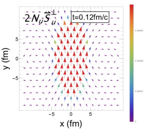
Figure 1: Transverse spin density of u quark $2N_{u}\vec{S}^{\perp}_{u}$ on the $x-y$ plane with $z=0$ at time $t=0.12\rm fm/c$ choosing the RTA $\tau_{R}=0.2\rm fm/c$.

Let’s next quantify the out-of-equilibrium spin polarization effect and study its dependence on various ingredients in the modeling. To quantify this effect, we will use y component $P_{y}$ of the spin polarization vector and y component $S_{y}(t)$ of the average spin vector, which have been defined in Eq.(5) and Eq.(II). In our calculations, we found that the x and z components of the spin polarization and the average spin vectors tend to be zero and can be ignored, consistent with the magnetic field source. The spin polarization $P_{y}$ is shown in Fig. 2 as a function of time t. The absolute of $P_{y}$ monotonically decays with time for all of the quarks, which is consistent with the decay of the magnetic field. However, interactions between quarks will affect the decay behavior of spin polarization. The weaker relaxation time, the stronger interaction. The right picture in Fig. 2 shows the comparison of spin polarization about u quark for different relaxation times, and reflects that the interaction will delay the decay of spin polarization at early stage, the stronger of interaction between quarks, the stronger delay. And then the interactions between the quarks accelerate the decay, and the stronger the interaction, the faster the decay. This reason is connected with the average spin vector, which will be described next.

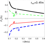
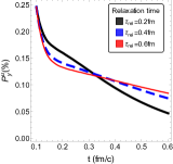
Figure 2: (left)The spin polarization of different quarks as a function of time, computed with the relaxation time $\tau_{R}=0.4\mathrm{fm}$. (right) Comparing the spin polarization of u quark for different relaxation time, $\tau_{R}=0.2,0.4,0.6\mathrm{fm}$.

It will be more explicit about the effect of interaction between quarks on the average spin vector. The average spin $S_{y}$ as a function of time is shown in Fig. 3. It shows the absolute average spin for all of the quarks monotonically increases to a peak around time $t=0.2\rm fm$, and then monotonically decays with time. As shown in the right part in Fig. 3, the average spin is very sensitive to the interaction between quarks. The stronger interaction between quarks, the faster increase to peak at an early time, and then faster decay from the peak. It is clear that the interaction between quarks on the average spin in the fireball is an accelerating effect, accelerating not only its growth but also its decay. The interaction between quarks will enhance the polarization of spin of quarks from zero average spin stage, and meantime it will destroy the polarization of spin. The average spin vector is the zeroth order part of spin polarization defined in Eq.(5) as mentioned before. Then one can be understood the reason of the behavior of spin polarization in the right-hand picture of Fig. 2.

We want to notice that the difference of the average spin (or spin polarization) for quark and anti-quark scaled by the quark charge is the same at any time during the evolution, i.e ${\Delta}S^{u}_{y}(t)/q_{u}={\Delta}S^{d}_{y}(t)/q_{d}$, or ${\Delta}P^{u}_{y}(t)/q_{u}={\Delta}P^{d}_{y}(t)/q_{d}$, where ${\Delta}S^{u}_{y}=S^{u}_{y}-S^{\bar{u}}_{y}$ and ${\Delta}P^{u}_{y}=P^{u}_{y}-P^{\bar{u}}_{y}$.

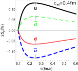
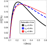
Figure 3: (left)The evolution picture of the average spin of different quarks, computed with the RTA $\tau_{R}=0.4\mathrm{fm}$. (right) Comparing the average spin of u quark for different RTA.

We next examine the influence of the interaction between quarks on the dynamical evolution of the magnetic field at an early stage in heavy-ion collisions. We plot the comparison of the external magnetic field $B^{ext}_{y}(t)$ and total magnetic field $B^{total}_{y}(t)=B^{ext}_{y}(t)+B^{int}_{y}(t)$ as a function of time computed for RTA $\tau_{R}=0.4\rm fm$ shown in the left part in Fig. 4. The external and total magnetic fields are almost identical, a result consistent with previous worksVoronyuk:2011jd ; Wang:2021oqq . This means that the induced (internal) magnetic field is very small at the early stage in heavy-ion collisions, and can be negligible compared to the external magnetic field. However, this conclusion does not prevent further studies on the evolution of magnetic fields in the early stages of heavy ion collisions. In this work, we have not yet considered some key factors, namely the net charge effect and the vorticity effect, both of which have a very large effect on the induced magnetic fieldGuo:2019mgh . At the same time, we found that the induced magnetic field is not very sensitive to the interactions between quarks, as shown in the right panel of Figure. 4. The results also show that there is an incomplete electromagnetic response effect, and the increase of the induced magnetic field in the direction opposite to the decay of the external magnetic field has a delay effect. In general, the induced magnetic field should be positive and increase rapidly to some ”stable” value.

However, the case of the fireball’s electromagnetic response is changed when the configuration of the external magnetic field is changed. Let’s try to make the external magnetic field decay slowly and keep the spatial distribution fixed. We then found that the induced magnetic field increases rapidly in the opposite direction to the decay of the external magnetic field, as shown in the figure. 5. Where we set the external magnetic field decay by the formula $B=B_{0}/(1+(t/t_{B})^{2})$, instead of decaying like the method described above, herein, $B_{0}$ is the magnetic field created by heavy-ions (as before) at time $t=0.0\rm\,fm$, the life of the magnetic field is set to $t_{B}=0.4\rm\,fm$. One can also find that the effect of the interaction between quarks on the induced magnetic field is more explicit in this case. The stronger of interaction, the stronger the induced magnetic field. This means that the induced magnetic field is strongly dependent on the decay rate and distribution of the external magnetic field.

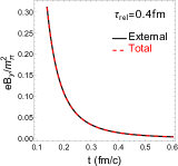
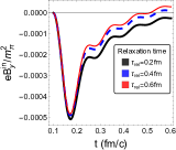
Figure 4: (left)The evolution picture of the external and total magnetic field at the center of the fireball, computed with the RTA $\tau_{R}=0.4\mathrm{fm}$. (right) Comparing the induced (internal) magnetic field for different RTA.

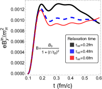
Figure 5: The induced (internal) magnetic field for different RTA calculated with the external magnetic field $B=B_{0}/(1+(t/t_{B})^{2})$, $B_{0}$ is the magnetic field created by heavy-ions (as before) at time $t=0.0\rm fm$, the life of magnetic field is set to $t_{B}=0.4\rm fm$.

V Summary

In summary, we have performed a phenomenological study of the magnetic-induced spin polarization of quarks and the dynamical magnetic field during the pre-thermal stage in heavy ion collisions. In such a collision, the extremely strong magnetic field may last only for a brief moment and the magnetic-induced spin polarization may occur at so early a stage that the quark-gluon matter is still far from thermal equilibrium. Utilizing the tool of chiral kinetic theory, we have shown the dynamical evolution of magnetic-induced spin polarization of QGP by the spin polarization and average spin of quarks and studied its dependence on various ingredients in the modeling. The effect is found to be sensitive to the relaxation time of the system evolution toward thermal equilibrium. In the present work, it is found that this pre-thermal magnetic-induced spin polarization is considerable.

In our simulation, we find that the magnetic-induced spin polarization monotonically decreases as the magnetic field decays. Interestingly, the interaction between quarks can delay the decay of spin polarization at an early stage but accelerate it later. However, the magnetic-induced average spin monotonically increases to a peak at first and then monotonically decays with time. The effect of interaction between quarks on the magnetic-induced average spin is an accelerating effect that not only accelerates its growth but also its decay. It enhances the average spin from zero at first and then accelerates its destruction later.

We also have shown the dynamical evolution of the induced magnetic field in a pre-thermal QGP and investigated its dependence on different relaxation times and the decay mode of the external field. The induced magnetic field is typically significantly weaker than the external magnetic field and may be considered negligible. It is not very sensitive to the interaction between quarks but is highly dependent on the decay rate and distribution of the external magnetic field. Furthermore, the electromagnetic response of the fireball at an early stage is incomplete, the increase of the induced magnetic field has a delayed effect.

The current study has inspired us to delve deeper into the dynamics of spin polarization and magnetic fields in lower-energy heavy-ion collisions. In such collisions, the external magnetic field decays more slowly due to the relatively slower movement of the projectile and target. Consequently, quarks experience a prolonged magnetic-induced spin polarization, which presents a unique opportunity for us to explore this phenomenon in greater detail. Based on the present work, we intend to develop a more comprehensive and realistic framework to study the dynamic evolution of the magnetic field and spin polarization in low-energy heavy-ion collisions in the future. This future work will be conducted by replacing the kinetic theory with chiral kinetic theory and incorporating Maxwell equations into the ZPC.f program of A Multi-Phase Transport(AMPT)Zhang:1999bd ; Lin:2001zk ; Lin:2002gc , which is employed to simulate the Parton cascade. This will allow us to delve deeper into this fascinating phenomenon and gain a better understanding of its underlying mechanisms.

Acknowledgments. The research of A.H. especially thanks to the support of the National Natural Science Foundation of China (NSFC) Grant No.12205309. The work is also supported by the the National Natural Science Foundation of China (NSFC) Grant No. 12235016 and No. 12221005, the Strategic Priority Research Program of Chinese Academy of Sciences Grant No. XDB34030000, the Fundamental Research Funds for the Central Universities.

References

- (1) Dmitri Kharzeev. Parity violation in hot QCD: Why it can happen, and how to look for it. Phys. Lett. B, 633:260–264, 2006.
- (2) D. Kharzeev and A. Zhitnitsky. Charge separation induced by P-odd bubbles in QCD matter. Nucl. Phys. A, 797:67–79, 2007.
- (3) Dmitri E. Kharzeev, Larry D. McLerran, and Harmen J. Warringa. The Effects of topological charge change in heavy ion collisions: ’Event by event P and CP violation’. Nucl. Phys. A, 803:227–253, 2008.
- (4) Kenji Fukushima, Dmitri E. Kharzeev, and Harmen J. Warringa. The Chiral Magnetic Effect. Phys. Rev. D, 78:074033, 2008.
- (5) Dmitri E. Kharzeev and Ho-Ung Yee. Chiral Magnetic Wave. Phys. Rev. D, 83:085007, 2011.
- (6) Yannis Burnier, Dmitri E. Kharzeev, Jinfeng Liao, and Ho-Ung Yee. Chiral magnetic wave at finite baryon density and the electric quadrupole moment of quark-gluon plasma in heavy ion collisions. Phys. Rev. Lett., 107:052303, 2011.
- (7) Dam T. Son and Piotr Surowka. Hydrodynamics with Triangle Anomalies. Phys. Rev. Lett., 103:191601, 2009.
- (8) Dmitri E. Kharzeev and Dam T. Son. Testing the chiral magnetic and chiral vortical effects in heavy ion collisions. Phys. Rev. Lett., 106:062301, 2011.
- (9) A. V. Sadofyev, V. I. Shevchenko, and V. I. Zakharov. Notes on chiral hydrodynamics within effective theory approach. Phys. Rev. D, 83:105025, 2011.
- (10) Karl Landsteiner, Eugenio Megias, Luis Melgar, and Francisco Pena-Benitez. Holographic Gravitational Anomaly and Chiral Vortical Effect. JHEP, 09:121, 2011.
- (11) Yin Jiang, Xu-Guang Huang, and Jinfeng Liao. Chiral vortical wave and induced flavor charge transport in a rotating quark-gluon plasma. Phys. Rev. D, 92(7):071501, 2015.
- (12) L. Adamczyk et al. Global hyperon polarization in nuclear collisions: evidence for the most vortical fluid. Nature, 548:62–65, 2017.
- (13) Jaroslav Adam et al. Global polarization of hyperons in Au+Au collisions at = 200 GeV. Phys. Rev. C, 98:014910, 2018.
- (14) Jaroslav Adam et al. Polarization of () hyperons along the beam direction in Au+Au collisions at = 200 GeV. Phys. Rev. Lett., 123(13):132301, 2019.
- (15) Takafumi Niida. Global and local polarization of hyperons in Au+Au collisions at 200 GeV from STAR. Nucl. Phys. A, 982:511–514, 2019.
- (16) Shreyasi Acharya et al. Global polarization of hyperons in Pb-Pb collisions at = 2.76 and 5.02 TeV. Phys. Rev. C, 101(4):044611, 2020. [Erratum: Phys.Rev.C 105, 029902 (2022)].
- (17) F. Becattini, V. Chandra, L. Del Zanna, and E. Grossi. Relativistic distribution function for particles with spin at local thermodynamical equilibrium. Annals Phys., 338:32–49, 2013.
- (18) Ren-hong Fang, Long-gang Pang, Qun Wang, and Xin-nian Wang. Polarization of massive fermions in a vortical fluid. Phys. Rev. C, 94(2):024904, 2016.
- (19) Long-Gang Pang, Hannah Petersen, Qun Wang, and Xin-Nian Wang. Vortical Fluid and Spin Correlations in High-Energy Heavy-Ion Collisions. Phys. Rev. Lett., 117(19):192301, 2016.
- (20) Shuai Y. F. Liu, Yifeng Sun, and Che Ming Ko. Spin Polarizations in a Covariant Angular-Momentum-Conserved Chiral Transport Model. Phys. Rev. Lett., 125(6):062301, 2020.
- (21) Hong-Zhong Wu, Long-Gang Pang, Xu-Guang Huang, and Qun Wang. Local spin polarization in high energy heavy ion collisions. Phys. Rev. Research., 1:033058, 2019.
- (22) Wojciech Florkowski, Avdhesh Kumar, Radoslaw Ryblewski, and Aleksas Mazeliauskas. Longitudinal spin polarization in a thermal model. Phys. Rev. C, 100(5):054907, 2019.
- (23) Baochi Fu, Shuai Y. F. Liu, Longgang Pang, Huichao Song, and Yi Yin. Shear-Induced Spin Polarization in Heavy-Ion Collisions. Phys. Rev. Lett., 127(14):142301, 2021.
- (24) Baochi Fu, Kai Xu, Xu-Guang Huang, and Huichao Song. Hydrodynamic study of hyperon spin polarization in relativistic heavy ion collisions. Phys. Rev. C, 103(2):024903, 2021.
- (25) Berndt Müller and Andreas Schäfer. Chiral magnetic effect and an experimental bound on the late time magnetic field strength. Phys. Rev. D, 98(7):071902, 2018.
- (26) Xingyu Guo, Jinfeng Liao, and Enke Wang. Spin Hydrodynamic Generation in the Charged Subatomic Swirl. Sci. Rep., 10(1):2196, 2020.
- (27) Yu Guo, Shuzhe Shi, Shengqin Feng, and Jinfeng Liao. Magnetic Field Induced Polarization Difference between Hyperons and Anti-hyperons. Phys. Lett. B, 798:134929, 2019.
- (28) Zhang-Zhu Han and Jun Xu. Charge asymmetry dependence of the elliptic flow splitting in relativistic heavy-ion collisions. Phys. Rev. C, 99(4):044915, 2019.
- (29) Francesco Becattini and Michael A. Lisa. Polarization and Vorticity in the Quark–Gluon Plasma. Ann. Rev. Nucl. Part. Sci., 70:395–423, 2020.
- (30) Kun Xu, Fan Lin, Anping Huang, and Mei Huang. /¯ polarization and splitting induced by rotation and magnetic field. Phys. Rev. D, 106(7):L071502, 2022.
- (31) M. A. Stephanov and Y. Yin. Chiral Kinetic Theory. Phys. Rev. Lett., 109:162001, 2012.
- (32) Dam Thanh Son and Naoki Yamamoto. Berry Curvature, Triangle Anomalies, and the Chiral Magnetic Effect in Fermi Liquids. Phys. Rev. Lett., 109:181602, 2012.
- (33) Dam Thanh Son and Naoki Yamamoto. Kinetic theory with Berry curvature from quantum field theories. Phys. Rev. D, 87(8):085016, 2013.
- (34) Jiunn-Wei Chen, Shi Pu, Qun Wang, and Xin-Nian Wang. Berry Curvature and Four-Dimensional Monopoles in the Relativistic Chiral Kinetic Equation. Phys. Rev. Lett., 110(26):262301, 2013.
- (35) Dmitri E. Kharzeev, Mikhail A. Stephanov, and Ho-Ung Yee. Anatomy of chiral magnetic effect in and out of equilibrium. Phys. Rev. D, 95(5):051901, 2017.
- (36) Yoshimasa Hidaka, Shi Pu, and Di-Lun Yang. Relativistic Chiral Kinetic Theory from Quantum Field Theories. Phys. Rev. D, 95(9):091901, 2017.
- (37) Niklas Mueller and Raju Venugopalan. Worldline construction of a covariant chiral kinetic theory. Phys. Rev. D, 96(1):016023, 2017.
- (38) E. V. Gorbar, V. A. Miransky, I. A. Shovkovy, and P. O. Sukhachov. Second-order chiral kinetic theory: Chiral magnetic and pseudomagnetic waves. Phys. Rev. B, 95(20):205141, 2017.
- (39) Anping Huang, Shuzhe Shi, Yin Jiang, Jinfeng Liao, and Pengfei Zhuang. Complete and Consistent Chiral Transport from Wigner Function Formalism. Phys. Rev. D, 98(3):036010, 2018.
- (40) L McLerran and V Skokov. Comments about the electromagnetic field in heavy-ion collisions. Nuclear Physics A, 929:184–190, 2014.
- (41) Anping Huang, Duan She, Shuzhe Shi, Mei Huang, and Jinfeng Liao. Dynamical magnetic fields in heavy-ion collisions. Phys. Rev. C, 107(3):034901, 2023.
- (42) Vasiliĭ Aristov. Direct methods for solving the Boltzmann equation and study of nonequilibrium flows.
- (43) Kane Yee. Numerical solution of initial boundary value problems involving maxwell’s equations in isotropic media. IEEE Transactions on antennas and propagation, 14(3):302–307, 1966.
- (44) Graeme A Bird. Molecular gas dynamics and the direct simulation of gas flows. Molecular gas dynamics and the direct simulation of gas flows, 1994.
- (45) Yu N Grigoryev and Vitaliĭ Vshivkov. Numerical” particle-in-cell” methods.
- (46) L. McLerran and V. Skokov. Comments About the Electromagnetic Field in Heavy-Ion Collisions. Nucl. Phys., A929:184–190, 2014.
- (47) B. G. Zakharov. Electromagnetic response of quark–gluon plasma in heavy-ion collisions. Phys. Lett. B, 737:262–266, 2014.
- (48) B Alver, M Baker, C Loizides, and P Steinberg. The phobos glauber monte carlo. arXiv preprint arXiv:0805.4411, 2008.
- (49) Kane Yee. Numerical solution of initial boundary value problems involving maxwell’s equations in isotropic media. IEEE Transactions on Antennas and Propagation, 14(3):302–307, 1966.
- (50) H. Kowalski, T. Lappi, and R. Venugopalan. Nuclear enhancement of universal dynamics of high parton densities. Phys. Rev. Lett., 100:022303, 2008.
- (51) Jean-Paul Blaizot, François Gelis, Jinfeng Liao, Larry McLerran, and Raju Venugopalan. Bose–einstein condensation and thermalization of the quark–gluon plasma. Nuclear Physics A, 873:68–80, 2012.
- (52) Jean-Paul Blaizot, Jinfeng Liao, and Larry McLerran. Gluon transport equation in the small angle approximation and the onset of bose–einstein condensation. Nuclear Physics A, 920:58–77, 2013.
- (53) Jean-Paul Blaizot, Bin Wu, and Li Yan. Quark production, bose–einstein condensates and thermalization of the quark–gluon plasma. Nuclear Physics A, 930:139–162, 2014.
- (54) Anping Huang, Yin Jiang, Shuzhe Shi, Jinfeng Liao, and Pengfei Zhuang. Out-of-equilibrium chiral magnetic effect from chiral kinetic theory. Phys. Lett. B, 777:177–183, 2018.
- (55) V. Voronyuk, V. D. Toneev, W. Cassing, E. L. Bratkovskaya, V. P. Konchakovski, and S. A. Voloshin. (Electro-)Magnetic field evolution in relativistic heavy-ion collisions. Phys. Rev. C, 83:054911, 2011.
- (56) Zeyan Wang, Jiaxing Zhao, Carsten Greiner, Zhe Xu, and Pengfei Zhuang. Incomplete electromagnetic response of hot QCD matter. Phys. Rev. C, 105(4):L041901, 2022.
- (57) Bin Zhang, C. M. Ko, Bao-An Li, and Zi-wei Lin. A multiphase transport model for nuclear collisions at RHIC. Phys. Rev. C, 61:067901, 2000.
- (58) Zi-wei Lin and C. M. Ko. Partonic effects on the elliptic flow at RHIC. Phys. Rev. C, 65:034904, 2002.
- (59) Zi-wei Lin, C. M. Ko, and Subrata Pal. Partonic effects on pion interferometry at RHIC. Phys. Rev. Lett., 89:152301, 2002.