Interaction renormalization and validity of kinetic equations for turbulent states

Vladimir Rosenhaus¹ and Gregory Falkovich²

UKvardate[] ,

¹ Initiative for the Theoretical Sciences
The Graduate Center, CUNY
365 Fifth Ave, New York, NY 10016, USA

²Weizmann Institute of Science
Rehovot 76100 Israel

We consider turbulence of waves that interact weakly via four-wave scattering (such as sea waves, plasma waves, spin waves, and many others). In the first non-vanishing order in the interaction, the occupation number of waves satisfies a closed kinetic equation. We show that a straightforward perturbation theory beyond the kinetic equation gives, at any wavenumber, terms that generally diverge – go to infinity when the maximum wavenumber (UV) goes to infinity or the minimum wavenumber (IR) goes to zero. Since the power of the UV divergence increases with the order, we identify and sum the series of the most divergent contributions to the fourth moment of complex wave amplitudes. This gives a new kinetic equation renormalized by multi-mode interactions. We show that the true dimensionless four-wave coupling is in general parametrically different from the naive estimate and that the effective interaction either decays or grows explosively with the extent of the cascade, depending on the sign of the new coupling. The explosive growth possibly signals the appearance of a multi-wave bound state (solitons, shocks, cusps) similar to confinement in quantum chromodynamics.

1.  Introduction

Kinetic equations are workhorses of physics and engineering. The most widely used are the Boltzmann equation for particles and the Peierls kinetic equation for waves. They describe transport phenomena and turbulence, from gas pipes and oceans, to plasmas in space and in thermonuclear reactors. These equations are so effective because they reduce the description of multi-particle or multi-wave systems to a closed equation on a single-particle probability distribution, or a single wavevector occupation number. The equations have solutions that describe different equilibria, transport in weakly non-equilibrium states, and even far-from-equilibrium turbulent states. The question is whether these solutions are physical, that is, if they also satisfy (with small modifications) the corrections to the kinetic equations due to multi-particle and multi-mode correlations.

This question was first addressed for the density expansion beyond the Boltzmann equation. One can show that this (virial) expansion is regular for thermal equilibria [1, 2]. For weakly non-equilibrium transport states, on the other hand, the expansion always introduces long-distance divergences [2, 3, 4, 5, 6]. To describe transport in a gas and compute kinetic coefficients (diffusivity, thermal conductivity, viscosity, etc.), one imposes a spatial gradient and computes the respective flux as a series in powers of the density. The first term is determined by the Boltzmann equation, that is, by the binary collisions. The higher-order terms, which involve subsequent collisions involving some of the same particles, necessarily contain spatial integrals over the possible positions of those collisions. These spatial integrals have infrared (IR) divergences starting from second order (in two dimensions) or from third order (in three dimensions). These divergences produce the memory effects creating long-distance multi-particle correlations. In thermal equilibrium, such divergences are canceled due to detailed balance, and the correlations are short, so that the equations of state have a regular virial expansion. Spatial non-equilibrium prevents cancelation.

Of course, the spatial IR divergences appear because the “naive” virial expansion allows particles to travel arbitrarily long distances between subsequent collisions. A properly renormalized expansion must account for the collective effects which impose the mean free path as an IR cutoff. The expansion then involves powers of density other than integers (adding density logarithms in this case). Such perturbation theory is singular, even though the corrections are small in dimensions exceeding two. The divergences lead to logarithmic renormalization of the kinetic coefficients in two dimensions and to anomalous kinetics in one dimension, which is a subject of active research.

In contrast to transport states, turbulent states deviate a system from thermal equilibrium by creating fluxes (cascades) in momentum space rather than in real space. The cascade distributions were found as exact (Zakharov) solutions of the kinetic equations both for particles and waves [7]. Such solutions require locality of interactions, which is the convergence of the collision integrals in the respective kinetic equations. Physically, this means that the contribution of the lowest-order collisions and interactions are predominantly given by comparable momenta of colliding particles or wavenumbers of interacting waves. The natural question is then whether locality also holds in the higher-order corrections to the kinetic equations [8, 11], which describe multi-particle collisions and multi-wave interactions. In this work, we answer this question in the negative, finding divergences in $k$-space (the space in which non-equilibrium now lives). The divergences are due to large momenta or wavenumber (UV), and the degree of divergence grows with the order of the coupling. We identify and sum the series of the most divergent terms. This allows us to derive a new renormalized kinetic equation, which has a new four-wave coupling renormalized by multi-wave interactions.

It is important to state from the beginning that the nature of renormalization in turbulence theory is quite different from that in quantum field theory or critical phenomena. There, one always deals with effective large-scale theories, describing how a bare value at some small UV scale (Planck scale or lattice spacing) is getting renormalized as one increases the scale of measurements. Quite distinctly, our bare values of the coefficients of the Hamiltonian (such as the frequency or the four-wave coupling) are given by the equations of motion which are uniformly valid on all scales, including at and below our UV cutoff, which is the dissipation scale of turbulence (where the time of attenuation due to external factors is comparable to the nonlinear interaction time). These bare values describe the frequency of a single wave propagating in an undisturbed medium, and the interaction energy of four waves without any other waves present. When turbulence is present, both the frequency and the four-wave coupling are renormalized. How this renormalization depends on the turbulence level and the extent in scales is the subject of this work. In quantum field theory, one cannot switch off quantum fluctuations, so the meaning of bare and renormalized values is different.

Using the renormalized kinetic equation, we are able to check whether the weakly turbulent Zakharov spectra satisfy the renormalized kinetic equation, if we keep the turbulence level small at a given $k$, increasing either the pumping scale or the dissipation wavenumber. The validity of the weak-turbulence approximation depends on the effective dimensionless coupling in the renormalized kinetic equation. We show that the effective coupling is generally different from the naive estimate, since it contains integrals that could diverge. For both classes of models that we are able to solve explicitly, the effective coupling always contains an IR divergence and could contain a UV divergence as well, depending on the asymptotics of the bare vertex. When the UV divergence is present, the corrections to the weakly turbulent solutions grow upon an increase of the dissipation wavenumber. This is a new phenomenon, neither observed nor predicted in turbulence before. When the UV divergence is absent, the corrections stay small when the dissipation wavenumber goes to infinity. In this case, the renormalized kinetic equation has a built-in UV cutoff due to collective effects restricting interactions with very short waves. Since the cutoff depends on the nonlinearity, this introduces non-integer powers of the coupling into the expansion. In other words, the perturbation theory exists, yet is singular, similar to the virial expansion for transport states mentioned earlier. On the other hand, the IR divergences make deviations from the weak turbulence approximation grow with an increase of the pumping scale $L$ (for a direct cascade). This introduces an explicit dependence on $L$, reminiscent of anomalous scaling in fluid turbulence, where the statistics at a given wavenumber $k$ deviates further and further from Gaussian as $kL$ increases. Could, similarly, a sufficiently long cascade interval $kL$ make weak wave turbulence strong, even at a small level of nonlinearity at a given $k$? To answer this question one needs to analyze the IR divergences in an analogous way to the analysis of the UV divergences here; this is left for future work.

The transition to strong turbulence upon the change of the effective coupling can be identified in the renormalized kinetic equation as being one of two types. When the effective coupling is positive, renormalization increases the strength of the vertex, which may lead to a pole at a finite $k$ in the renormalized kinetic equation (similar to quantum chromodynamics). We hypothesize that in this case the renormalized kinetic equation has a cascade solution that starts from a weakly turbulent spectrum at low wavenumbers and turns at large wavenumbers into a universal (pumping-independent) spectrum dominated by bound states of many correlated harmonics (long lived like solitons and shocks, or transient like wave collapses). When the effective coupling is negative, like in quantum electrodynamics, the strong-turbulence spectrum is likely to be flux-dependent.

Perhaps the most physically appealing aspect of our results is a criterion for the sign of the effective coupling. Note that the bare coupling generally changes sign depending on the configurations of the four wave vectors, as is the case, for instance, for surface water waves. We show that when the effective coupling is given by a UV-convergent and IR-divergent integral, it is positive if the sign of the wave dispersion is opposite to that of the bare coupling integrated over all wave vectors, weighted by the turbulence spectrum. This is a nonlocal turbulent analog of the single-wave criterion for modulational instability, which also signals the possibility of bound states (solitons and wave collapses). That this criterion has a generalization, from a single wave to turbulence, seems remarkable.

2.  The model

We consider particles/quasiparticles with energy/frequency $\omega_{k}=k^{\alpha}$, which interact via four-wave scattering described by the Hamiltonian

$$H=\sum_{p}\omega_{p}a_{p}^{*}a_{p}+\sum_{p_{1},p_{2},p_{3},p_{4}}\!\!\lambda_{p_{1}p_{2}p_{3}p_{4}}\delta({\bf p_{1}}{+}{\bf p_{2}}{-}{\bf p_{3}}{-}{\bf p_{4}})a_{p_{1}}^{*}a_{p_{2}}^{*}a_{p_{3}}a_{p_{4}}~{}.$$ (2.1)

The complex amplitudes $a_{p}$ are normal canonical variables that satisfy the equations of motion $ida_{k}/dt=\partial H/\partial a_{k}^{*}$. The real vertex $\lambda_{1234}\equiv\lambda_{p_{1}p_{2}p_{3}p_{4}}$ can be of either sign and is a homogeneous function of degree $\beta$: $\lambda_{ap_{1}ap_{2}ap_{3}ap_{4}}=a^{\beta}\lambda_{p_{1}p_{2}p_{3}p_{4}}$. The vertex $\lambda_{1234}$ can be complex for systems with rotation or for a plasma in a magnetic field; Modifying our equations for the more general case is straightforward. In what follows we shall omit the delta function of the wave vectors. The kinetic equation describes the time derivative of the occupation numbers $n_{k}=\langle|a_{k}|^{2}\rangle$. Using the equations of motion, this can be expressed in terms of the four-point correlation function,

$${\partial n_{k}(t)\over\partial t}=I_{k}=4\sum_{p_{1},\ldots,p_{4}}\delta_{kp_{1}}\lambda_{p_{3}p_{4}p_{1}p_{2}}\text{Im}\langle a_{p_{1}}^{*}a_{p_{2}}^{*}a_{p_{3}}a_{p_{4}}\rangle~{}.$$ (2.2)

The equal-time four-point function in (2.2) can be found perturbatively as a series in $\lambda$, assuming that the statistics of the wave field is close to the Gaussian statistics of non-correlated waves, ${\cal P}\{a_{k}\}\propto\exp[-\sum_{k}|a_{k}|^{2}/n_{k}]$, which is completely determined by the occupation numbers. That provides the zeroth-order approximation, where the right-hand site of (2.2) is zero. A standard way to keep the distribution close to Gausssian and compute average corrections is to add infinitesimal forcing and dissipation to the equation of motion,

$$\frac{da_{k}}{dt}=-i\partial H/\partial a_{k}^{*}+f_{k}(t)-\gamma_{k}a_{k}\,.$$ (2.3)

The force is taken to be white in time and acting on each mode independently: $\langle f_{k}(0)f_{q}(t)\rangle=F_{k}\delta(k{-}q)\delta(t)$. At the end of the computation one takes the limit $F_{k},\gamma_{k}\to 0$, while keeping $F_{k}/2\gamma_{k}=n_{k}$ finite. The respective standard Wyld diagram technique was introduced in [9], applied to wave turbulence in [10], and given a modern compact form in [8], see Appendix B. Acting by an independent random force $f_{k}$ on every mode is natural in thermal equilibrium, where one uses the equipartition occupation numbers, $n_{k}\omega_{k}=$const. Starting from [10], one also uses this way of averaging for arbitrary $n_{k}$. There are always factors in the environment which scramble phase correlations; modeling them by an infinitesimal white force is an artifical yet legitimate option. It is reinforced by the fact that the kinetic equation obtained this way does have turbulent Zakharov exact solutions, described below.

In such a straightforward (naive) perturbation theory, one takes the temporal Fourier transform and writes the solution of (2.3) as a series in $\lambda$. Denoting $q=(k,\omega)$ one gets:

$$[i(\omega_{k}{-}\omega)+\gamma_{k}]a_{q}=f_{q}-i\int{dq_{1}dq_{2}dq_{3}\over(2\pi)^{2}}\,\delta(q{+}q_{1}{-}q_{2}{-}q_{3})\lambda_{k123}a_{q_{1}}^{*}a_{q_{2}}a_{q_{3}}$$

$$\approx f_{q}-i\int{dq_{1}dq_{2}dq_{3}\over(2\pi)^{2}}\delta(q{+}q_{1}{-}q_{2}{-}q_{3}){\lambda_{k123}f_{q_{1}}^{*}\over\gamma_{1}-i(\omega_{k_{1}}\!-\omega_{1})}\,{f_{q_{2}}\over i(\omega_{k_{2}}\!-\omega_{2})+\gamma_{2}}\,{f_{q_{3}}\over i(\omega_{k_{3}}\!-\omega_{3})+\gamma_{3}}+O(\lambda^{2})\,.$$

Multiplying such expressions and averaging over $f_{q}$, one obtains the first non-vanishing contribution to the fourth moment in (2.2), which could be symbolically depicted as the tree-level diagram shown in Figure 1. This gives the standard kinetic equation:

$${\partial n_{k}(t)\over\partial t}=16\sum_{p_{1},\ldots,p_{4}}\delta_{k,p_{1}}\pi\delta(\omega_{p_{1}p_{2};p_{3}p_{4}})\lambda_{1234}^{2}n_{1}n_{2}n_{3}n_{4}\,\Big{(}\frac{1}{n_{1}}{+}\frac{1}{n_{2}}{-}\frac{1}{n_{3}}{-}\frac{1}{n_{4}}\Big{)}~{},$$ (2.4)

where we defined $\omega_{p_{i}p_{j};p_{k}p_{l}}\equiv\omega_{p_{i}}{+}\omega_{p_{j}}{-}\omega_{p_{k}}{-}\omega_{p_{l}}$. Note that in the kinetic equations, both the wave kinetic equation (2.4) and the Boltzmann equation, the rate of change of the occupation numbers is determined by their instantaneous values.

What is traditionally required for the validity of the wave kinetic equation is not only to take the limit $\lambda_{1234}\to 0$, but also to provide a dense enough set of resonances, $\omega_{p_{1}}{+}\omega_{p_{1}}{-}\omega_{p_{3}}{-}\omega_{p_{4}}=0$, which requires taking the limit $kL\to\infty$, where $L$ is the box size, see e.g. [12, 13, 14]. This fact already requires a careful analysis of divergences in the kinetic equation and in the corrections to it.

Figure 1: The leading order kinetic equation (2.4) encodes the tree-level process of two modes directly scattering into two other modes.

The most important property of $\lambda_{1234}$ for the analysis of divergences will be its asymptotics when one or two wavenumbers become much smaller than the others. We shall do direct computations for two simple, yet representative, cases of $\lambda_{1234}$, having product and sum factorization of the bare vertex, respectively:

$$\lambda_{1234}=\sqrt{\lambda_{12}\lambda_{34}}~{},$$ (2.5)

$$\lambda_{1234}=\lambda_{12}+\lambda_{34}~{},$$ (2.6)

where $\lambda_{ij}$ only depends on $p_{i}$ and $p_{j}$. Literally, the first case (2.5) takes place, for instance, for optical turbulence with $\beta{=}0$; it can also be a qualitatively correct approximation for many other cases, such as for plasma turbulence with $\beta{=}\alpha{=}2$. The second case (2.6) of sum factorization takes place for spin waves with exchange interaction, where $\lambda_{12}=-\lambda(\vec{p}_{1}\cdot\vec{p}_{2})$ [7]. The consideration of these two cases will illustrate below to what extent turbulence depends on the specific form of $\lambda_{1234}$. We define three asymptotics:

$$\lim_{p_{1},p_{3}\ll p_{2},p_{4}}\lambda_{1234}=\lambda(p_{2}p_{4})^{\beta_{1}/2}(p_{1}p_{3})^{(\beta-\beta_{1})/2}\,.$$ (2.7)

$$\lim_{p_{1},p_{2}\ll p_{3},p_{4}}\lambda_{1234}=\lambda(p_{3}p_{4})^{\beta_{2}/2}(p_{1}p_{3})^{(\beta-\beta_{2})/2}\,.$$ (2.8)

$$\lim_{p_{1},p_{3},p_{4}\gg p_{2}}\lambda_{1234}\propto p_{2}^{\beta_{3}}~{}.$$ (2.9)

For (2.5), $\beta_{3}=\beta_{1}/2$, $\beta_{2}=\beta/2$. For (2.6), $2\beta_{1}=\beta_{2}=\beta$ and $\beta_{3}=0$, except for spin waves where $\alpha=2$, so that $\lim_{p_{2}\to 0}(\vec{p}_{3}{\cdot}\vec{p}_{4})\propto p_{2}$ and $\beta_{3}=1$. In some cases, $\beta_{1}\leq\beta/2$, which provides stronger convergence than might be expected on dimensional grounds. For surface water waves, $\beta=3$, $\beta_{1}=1$, and $\beta_{3}=3/4$.

The leading-order kinetic equation (2.4) has two integrals of motion: energy $\int\omega_{k}n_{k}\,d\vec{k}$ and wave action $\int n_{k}\,d\vec{k}$. It thus has two stationary solutions which describe turbulent cascades. Here we focus on the direct energy cascade (from small to large wavenumbers). Writing (2.4) as the energy continuity equation, $k^{d-1}\omega_{k}{\partial n_{k}/\partial t}=-\partial P_{k}/\partial\vec{k}$, and requiring the spectral flux to be constant, $P_{k}=P$, we obtain by power counting $P_{k}\propto k^{2\beta+3d}n_{k}^{3}$, which gives

$$n_{k}=k^{-\gamma}=k^{-d-2\beta/3}~{}.$$ (2.10)

Here we have chosen the flux value so as to get a factor of unity in front. One can also obtain (2.10) by estimating the flux $P$ as the energy density $\omega_{k}n_{k}k^{d}$ divided by the nonlinear interaction time $1/\omega_{k}\epsilon_{k}^{2}$, where the definition of $\epsilon_{k}$ is given below in (2.11). The existence of this $n_{k}$ as a stationary solution presumes locality, that is, convergence of the integrals in (2.4) upon substituting (2.10). The convergence conditions are somewhat different depending on the sign of $\alpha{-}1$ (the details can be found in the Appendix A and [15]). For $\alpha{<}1$, the combination of the IR and UV conditions gives $d{+}1{+}2\beta_{1}{-}2\alpha{<}\gamma{<}d{+}\beta{-}\beta_{1}{+}1{-}\alpha/2$. For the energy cascade, $\gamma{=}d{+}2\beta/3$, this requires $2(\beta_{1}{-}\beta/3){+}1{-}2\alpha<0<\beta/3{-}\beta_{1}{+}1{-}\alpha/2$ or $(\beta_{1}{-}\beta/3){<}\alpha/2$, which is satisfied for water waves. In the opposite case, $\alpha{>}1$, we have $d{+}1{+}2\beta_{1}{-}2\alpha{<}\gamma{<}d{+}2\beta_{3}$. For the energy cascade, this takes the form $1{+}2\beta_{1}{-}2\alpha{<}2\beta/3{<}2\beta_{3}$. This condition is satisfied for spin waves with $\beta=\alpha=2$ and $\beta_{3}=1$. Optical and plasmon turbulence in a nonisothermal plasma with $\alpha=2$, $\beta=0$ are IR borderline.

It is important to stress the peculiar nature of the kinetic equations (both our equation for waves and the Boltzmann kinetic equation for particles), which provides for the locality of turbulent cascades. Substituting a power law $n_{k}=k^{-\gamma}$ into the collision integrals, one might have naively expected divergences at least at one end (or both). However, the structure of the leading-order kinetic equation guarantees cancellations, one in the UV and two in the IR, which provide a locality window for $\gamma$ [7]. We will see that the locality window is generally absent for higher-order scattering processes in naive perturbation theory.

Assuming for the sake of power counting the scaling, $\omega_{k}=k^{\alpha}$, $\lambda_{kkkk}\simeq\lambda k^{\beta}$ and $n_{k}=k^{-\gamma}$, the dimensionless parameter of nonlinearity (coupling) at a given $k$ is expected to be

$$\epsilon_{k}=\frac{\lambda_{kkkk}n_{k}k^{d}}{\omega_{k}}\simeq\lambda k^{d+\beta-\gamma-\alpha}=\lambda k^{\beta/3-\alpha}=\epsilon_{0}\left({k\over k_{0}}\right)^{\beta/3-\alpha}~{}.$$ (2.11)

The standard claim is that (2.4) is valid and (2.10) is its solution for those $k$ for which $\epsilon_{k}\ll 1$ and under the above conditions of locality [7, 16]. Here locality means convergence of the integrals in the kinetic equation, which is expected to guarantee that the solution does not depend on $k_{0}$ (the IR cutoff) and $k_{max}$ (the UV cutoff) in the limits $k_{0}/k\to 0$ and $k/k_{max}\to 0$. For $\alpha\leq 1$ and in the simplest case (2.5), $\beta_{1}=\beta/2$, the convergence condition $\beta/3\leq\alpha$ also guarantees that the nonlinearity parameter $\epsilon_{k}$ decays with $k$, making it seem as if the weak turbulence approximation only gets better along the cascade. We will show that, in general, this is wrong: for wide classes of systems the higher order terms due to multi-mode interactions become progressively more and more divergent, so the validity of weak turbulence needs re-examination. In this work, the main focus is on UV divergences and on the limit $k_{max}\to\infty$.

When $\beta>3\alpha$ and $\epsilon_{k}$ grows along the cascade, on dimensional grounds one might have expected strong turbulence to appear at those $k$ for which $\epsilon_{k}\simeq 1$. We will show below that the effective dimensionless coupling is always parametrically larger than $\epsilon_{k}$, so that strong turbulence must start at lower $k$ than had been expected. We even find cases where it is enough to have $\epsilon_{k_{max}}\simeq 1$ to have strong turbulence even for $k\ll k_{max}$ where $\epsilon_{k}\ll 1$. There are two seemingly plausible scenarios for the character of strong turbulence depending on the scaling of $\omega_{k}$ and the form of $\lambda_{1234}$. The first is a qualitatively similar cascade, just with the weak-turbulence time, $1/\omega_{k}\epsilon_{k}^{2}$ replaced by the nonlinear time $1/\omega_{k}\epsilon_{k}=1/\lambda_{k}n_{k}k^{d}$, so that the spectral energy flux $P$ is estimated as the spectral density $\widetilde{\omega}_{k}n_{k}k^{d}$ divided by the nonlinear time, $P\simeq\widetilde{\omega}_{k}n_{k}k^{d}\lambda_{k}n_{k}k^{d}$, which gives $n_{k}\simeq(P/\lambda_{k}\widetilde{\omega}_{k})^{1/2}k^{-d}$. Here the renormalized frequency is $\widetilde{\omega}_{k}=\omega_{k}+\sum_{\bf q}\lambda_{kqkq}n_{q}$. The second scenario is the often suggested hypothesis of critical balance $\epsilon_{k}=$const, which gives the universal (flux-independent) spectrum $n_{k}\simeq k^{-d}\omega_{k}/\lambda_{k}$, see e.g. [17, 18, 19, 20]. Neither of these scenarios have ever been derived analytically, nor has any criterion been suggested for choosing between them for a given system. The renormalized kinetic equation we will derive below could have solutions of two kinds, a flux-dependent spectrum and a universal spectrum, depending on the sign of the effective coupling. Therefore, our derivation of the effective coupling sheds light on the nature of strong turbulence in different systems.

3.  Next-to-leading order

The simplest correction replaces the bare frequencies in the kinetic equation by the renormalized ones: $\widetilde{\omega}_{k}=\omega_{k}+\sum_{\bf q}\lambda_{kqkq}n_{q}$. The integral $\int\lambda_{kqkq}q^{-d-2\beta/3}d{\bf q}$ always converges in the UV, whereas it converges in the IR if $\beta/3{>}\beta_{1}$. When there is IR convergence, the first-order relative frequency renormalization is small and can be neglected: $\widetilde{\omega}_{k}/k^{\alpha}{-}1\simeq\epsilon_{k}\ll 1$. Such is the case for surface water waves, for instance, where $\lambda_{kqkq}\propto q({\vec{k}\cdot\vec{q}})$ for $q\ll k$. In some cases, however, there is an IR divergence. For example, (2.6) gives $\beta_{1}=\beta$. When $\beta_{1}\geq\beta/3$, there is a power law IR divergence already for the first-order frequency renormalization. If, in addition, $\beta_{1}>\alpha$ then, regardless of how small $\lambda$ may be, there will be a sufficiently large momentum $k_{*}$ for which the one-loop correction to the frequency is comparable to the bare frequency: $k_{*}\simeq\bigl{(}\lambda k_{0}^{\beta/3-\beta_{1}}\bigr{)}^{1/(\alpha-\beta_{1})}\simeq k_{0}\epsilon_{k}^{3/(\beta-3\beta_{1})}$, where we expressed $\lambda$ via $\epsilon_{k}$ from (2.11). Moreover, higher-order corrections to the Green functions have increasingly higher powers of divergence, as discussed in the Appendix B.5. The complete analysis of the IR divergences will be addressed elsewhere; the main subject of this work is UV divergences, which appear in the corrections to the interaction vertex.

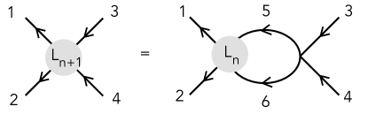
The next-to-leading order renormalization of the quartic interaction gives the two contributions to $\partial n_{k}/\partial t$, shown in Fig. 2, and given by [8, 11]:

$$64\pi\sum_{p_{1},\ldots,p_{6}}\delta_{k,p_{1}}\delta(\omega_{p_{1}p_{2};p_{3}p_{4}})\prod_{i=1}^{6}n_{i}\,\frac{\lambda_{3412}\lambda_{1256}\lambda_{5634}}{\omega_{p_{1}p_{2};p_{5}p_{6}}}\Big{(}\frac{1}{n_{1}}{+}\frac{1}{n_{2}}{-}\frac{1}{n_{3}}{-}\frac{1}{n_{4}}\Big{)}\Big{(}\frac{1}{n_{5}}{+}\frac{1}{n_{6}}\Big{)}+$$ (3.1)

$$256\pi\sum_{p_{1},\ldots,p_{6}}\delta_{k,p_{1}}\delta(\omega_{p_{1}p_{2};p_{3}p_{4}})\prod_{i=1}^{6}n_{i}\,\frac{\lambda_{3412}\lambda_{1635}\lambda_{2546}}{\omega_{p_{4}p_{6};p_{2}p_{5}}}\Big{(}\frac{1}{n_{1}}{+}\frac{1}{n_{2}}{-}\frac{1}{n_{3}}{-}\frac{1}{n_{4}}\Big{)}\Big{(}\frac{1}{n_{5}}{-}\frac{1}{n_{6}}\Big{)}\,.$$ (3.2)

The integral of $1/\omega$ is meant as the principal value part. Both these terms manifestly vanish for thermal equilibrium, $n_{k}\sim 1/(\omega_{k}{+}\mu)$, as they should. Indeed, the corrections at all order vanish on the thermal equipartition solution. This is not so for the turbulent solution.

(a)

(b)

Figure 2: The $\lambda^{3}$-terms in the kinetic equation, (3.1) and (3.2). They have the form of bubble diagrams and encode the scattering of the modes $p_{1},p_{2}$ onto $p_{3},p_{4}$ indirectly, by first scattering into modes $p_{5}$ and $p_{6}$. For small $\lambda_{1234}$, these terms would naively seem to be small relative to the tree-level diagram Fig, 1. However, for (a) there is an enhancement for $p_{2}\gg p_{1}$. This UV divergent contribution to the kinetic equation requires considering processes of all orders, discussed in the next section.

Let us now substitute the weak-turbulence spectrum $n_{k}=k^{-d-2\beta/3}$ into (3.1,3.2) and compare convergence of these terms with the leading order term in the kinetic equation, given earlier in (2.4). There are two new convergence issues here: an extra (loop) integration over $p_{5}$ and extra powers of $p_{2},p_{3},p_{4}$ in the external integration. The loop integration is IR-divergent under the same condition $\beta_{1}\geq\beta/3$ as for $\widetilde{\omega}_{k}$, which will be briefly addressed in Section 5 below. Generally, we keep the IR cutoff (pumping scale) finite in this work. Our main subject if what happens when UV cutoff $k_{max}$ goes to infinity. The extra integration over $p_{5}$ converges in the UV when $2\beta_{2}-2\beta/3-\alpha\leq 0$. For the product-factorized coupling (2.5) with $\beta_{2}=\beta/2$, this condition is satisfied for all cases that we know of. For the sum-factorized coupling (2.6), $\beta_{2}=\beta$, and UV divergence of the loop integration is possible, see the discussion in Sections 5,8. Here we focus on cumulative UV divergences: When $p_{2}$ is large, momentum conservation forces $p_{4}$ and $p_{6}$ to be large as well. Appendix A gives necessary background for the following discussion. In the limit $p_{2},p_{4},p_{6}\rightarrow\infty$, we have $\lambda_{1256}\lambda_{5634}/\lambda_{1234}\sim p_{2}^{\beta_{1}}$ and ${\omega_{p_{1},p_{2};p_{5},p_{6}}}\sim p_{2}^{-\max\{0,\alpha-1\}}$. We denote $\kappa=\max\{0,\alpha-1\}\geq 0$. Thus the extra term in (3.1) relative to (2.4) adds another factor of $p_{2}^{\beta_{1}-\kappa}$ to the integrand in (A.3), i.e. the right-hand side of the next-to-leading order kinetic equation in the UV (large $p_{2}$) is

$$\int^{k_{max}}d^{d}p_{2}\,p_{2}^{2\beta_{1}-\gamma-\alpha-\kappa+(\beta_{1}-\kappa)}~{}.$$ (3.3)

There is a divergence if

$$d{+}2\beta_{1}{-}\gamma{-}\alpha{-}\kappa{+}(\beta_{1}{-}\kappa)=3\beta_{1}{-}2\beta/3{-}2\kappa>0~{}.$$ (3.4)

When $\alpha>1$, the correction diverges when $3\beta_{1}-2\beta/3+2(1-\alpha)>0$. When $\alpha<1$, the divergence condition is

$$d{+}3\beta_{1}{-}\alpha-\gamma=3\beta_{1}{-}2\beta/3>0~{}.$$ (3.5)

For surface gravity waves, which have $\alpha=1/2$ and $\beta_{1}=1=\beta/3$, this correction term already diverges. When there is a divergence, the respective relative correction exceeds the dimensionless estimate $\epsilon_{k}$.

Our discussion was for the (bare) order $\lambda^{3}$ term. Going to higher orders, one finds that there are corrections to the fourth moment which generically at every order add the same extra degree of UV divergence: $\beta_{1}-\kappa$. This is independent of the spectrum exponent, so it applies for both the direct and inverse cascades. As a result, naive perturbation theory for $\alpha>1$ is valid only if

$$\beta_{1}-\kappa<0~{}.$$ (3.6)

This condition is satisfied for the nonlinear Schrödinger equation, which has $\alpha=2$ and $\beta=0$, and for the turbulence of gravitational waves in the early Universe, which can be shown to have $\alpha=1$, $\beta=0$, $\beta_{1}=-1$ [21]. For plasma turbulence with $\alpha=2$, $\beta_{1}=1$, we have logarithmic divergences at all orders.

For $\alpha\leq 1$, (3.5) shows that every order adds the degree of UV divergence $\beta_{1}\geq 0$, that is, naive perturbation theory is never valid, since it always involves divergent terms. This includes, in particular, turbulence of surface water waves and sound.

In what follows we analyze perturbation theory with UV divergences, assuming

$$\beta_{1}\geq\kappa=\max\{0,\alpha{-}1\}\,.$$ (3.7)

Our goal is to derive the renormalized kinetic equation up to order $\lambda^{3}$, and to arbitrary order in $k_{max}/k$.

To conclude this section, we computed the order $\lambda^{3}$ contribution to the collision integral of the kinetic equation (that is, to the fourth cumulant) and found a UV divergence. This is a sign that naive perturbation theory in terms of plane waves is inadequate, and we need to account for collective effects, which renormalize our four-wave interaction. This requires us to sum the most divergent diagrams at each order, which will cure the $\lambda^{3}$-divergence. As is familiar in quantum field theory, each of these diagrams will individually have a UV divergence, but their sum will be UV finite. Of course, this can be guaranteed only for the order $\lambda^{3}$ term in this new, renormalized, kinetic equation. If some of the diagrams at order $\lambda^{4}$ not included in our summation will also diverge, we again need to sum some class of diagrams to cure this. It may be that we already essentially did the necessary sum at the previous order (from our “renormalization” at order $\lambda^{3}$), but it may be that there is a different series of diagrams that need to be summed in addition. And so on to higher order. In the language of QFT, the theory is renormalizable if at some finite order in $\lambda$ there will be no new series of diagrams that need to be summed. Analyzing renormalizibility of weak turbulence is beyond the scope of the present work. Here we only deal with the renormalization of the collision integral of the kinetic equation, which is an integral of a single-time fourth moment of wave amplitudes.

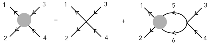
4.  Vertex renormalization by cumulative UV divergences

The leading UV divergences in the corrections to the kinetic equation found in the previous section form a subsequence of bubble diagrams, such as the ones shown in Fig. 3. The sum of the diagrams is computed in Appendix B, giving the Schwinger-Dyson integral equation for the fourth moment (B.11) in the momentum-frequency domain. We were able to solve this equation only in the two simple cases of a product-factorized and a sum-factorized vertex, see (B.13) and (B.47). Both solutions have leading terms, proportional to $({n_{1}}^{-1}{+}{n_{2}}^{-1})$ and $({n_{3}}^{-1}{+}{n_{4}}^{-1})$, and subleading terms (having an extra $\lambda$-factor) proportional to $({n_{1}}^{{-}1}{+}{n_{2}}^{-1})({n_{3}}^{-1}{+}{n_{4}}^{-1})$. Taking into account only the leading terms, one can explicitly integrate over frequencies, obtaining a renormalization of the single-time fourth moment, which could be presented as the renormalization of the four-wave vertex. The property which singles out the leading terms can be formulated in the language of old-fashioned perturbation theory as follows: For each Feynman diagram one considers all possible time orderings of the internal vertices (each of these corresponds to a different intermediate state). The terms we need are contained in the time ordering in which the times are monotonic between neighboring vertices in Fig. 3(a), so either all times are increasing or all times are decreasing, as one moves from left to right.

(a)

(b)

Figure 3: (a) We sum all the bubble diagrams contributing to the fourth moment of the amplitudes. The most divergent diagrams have within each bubble one line with a large momentum. (b) The kinetic equation (2.2) involves the moments with three of the four external momenta summed as well; we illustrate this by bringing together the external legs.

In more detail, to compute the leading contribution to the fourth moment $\langle a_{1}a_{2}a_{3}^{*}a_{4}^{*}\rangle$, we take the bubble diagrams in which the arrows in the loops run parallel; the diagrams with anti-parallel arrows in the loops are subleading in the limit of large momentum because they contain a difference of occupation numbers with close momenta. The diagram in Fig. 3(a) with $m$ loops gives an order $\lambda^{m+2}$ contribution to the kinetic equation. Each bubble gives a large contribution to the four-point function when the external momentum ($p_{2}$) becomes large, which leads to a UV divergence of the integration over $p_{2},p_{3},p_{4}$ in the kinetic equation. In addition, each diagram has an IR divergence, due to the internal loop integrals over $p_{5}$ (see Fig. 2(a)) being dominated by low momenta.

For such diagrams, the addition of one more loop replaces (see Appendix B.4),

$$\lambda_{j{-}1,j,3,4}\rightarrow\sum_{p_{j{+}1},p_{j{+}2}}\!\!\!\lambda_{j{-}1,j,j{+}1,j{+}2}\lambda_{j{+}1,j{+}2,3,4}n_{j{+}1}n_{j{+}2}\Big{(}\frac{1}{n_{j{+}1}}+\frac{1}{n_{j{+}2}}\Big{)}\frac{1}{\omega_{p_{3}p_{4};p_{j{+}1},p_{j{+}2}}{+}i\epsilon}~{}.$$ (4.1)

Therefore, the contribution to the equal-time fourth moment coming from the whole series of the time-ordered bubble diagrams involves an effective four-wave vertex renormalization, from $\lambda_{1234}$ to $T_{1234}$, where the (generally complicated) renormalized vertex $T_{1234}$, a function of the momenta $p_{1},p_{2},p_{3},p_{4}$, is the solution to the integral equation,

$$T_{1234}=\lambda_{1234}+\sum_{p_{5}p_{6}}\lambda_{1256}T_{5634}\frac{2(n_{5}{+}n_{6})}{\omega_{p_{3}p_{4};p_{5}p_{6}}{+}i\epsilon}\ .$$ (4.2)

We stress that $T_{1234}$ should not be viewed as the general renormalized quartic interaction — the statement is only that the equal-time fourth moment (which enters the kinetic equation), after accounting for leading loop diagrams, looks like the tree-level fourth moment but with $\lambda_{1234}$ replaced by $T_{1234}$. In particular, our usage of “renormalized coupling” is informal. In more direct language, our statement is that after computing the leading loop corrections to the tree-level kinetic equation, we find that the leading term of the renormalized kinetic equation takes the same form as the tree-level kinetic equation provided one replaces $\lambda_{1234}$ with $T_{1234}$.

Let us stress that neither the equation for the renormalized fourth moment in momentum-frequency space (B.11) nor the momentum-only equation (4.2) are exact. First, they presume small $\lambda_{1234}$ and are valid up to $\lambda^{3}$-terms. Second, they faithfully describe the renormalization of the fourth moment $\langle a_{1}a_{2}a_{3}^{*}a_{4}^{*}\rangle$ only when $p_{2},p_{4}\gg p_{1},p_{3}$, that is, in the regions where corrections to the kinetic equation diverge in the UV. But it is precisely in those regions where we need the renormalization, since in the rest of the momentum space the corrections are small and their form is irrelevant. The accounting of only leading (most UV-divergent) terms is likely a reason for the remarkable feat of obtaining a vertex renormalization (4.2) depending only on momenta, but not frequencies. In other words, the renormalized single-time fourth moment is expressed via the single-time second moments (occupation numbers) at the same time. Appendix B shows explicitly how all the integrations over frequencies are done, leading to such locality. Note that the second moments appearing there are all effectively taken to be bare: $n_{k\omega}=\delta(\omega-\omega_{k})F_{k}/2\gamma_{k}$.

To avoid misunderstanding and unwarranted optimism, it is important to state that there is no reason to expect a closed description of the whole single-time statistics in turbulence, where detailed balance is broken. In distinction from thermal equilibrium, single-time statistics is intimately related to different-time correlations in turbulence. What we found is the particular fact that the equation on the occupation numbers remains local in time even after adding the infinite series of the most UV-divergent corrections. As shown in Appendix B, this is true only for the leading in $\lambda$ contribution, which comes out of the time-ordered subsequence of the bubble diagrams.

From equation (4.2) one can see that the UV divergence at $p_{2},p_{4}\to\infty$ is cured for the new vertex, since $T_{1234}$ cannot grow with $p_{2},p_{4}$ faster than $\lambda_{1234}$. Indeed, for not very large $p_{2},p_{4}$ we have $T_{1234}\approx\lambda_{1234}$, while $T_{1234}$ cannot grow at all for very large $p_{2},p_{4}$, because then the last term in (4.2) cannot be compensated.

The saturation of the renormalized vertex can be seen, in particular, from the explicit solutions of (4.2), which can be found for simple functional forms of the bare vertex. Let us define for $r=0,1,2$ the loop integrals, see Fig. 2(a)

$$\mathcal{L}_{r}(p_{3},p_{4})=\sum_{p_{5}}\lambda_{56}^{r}\frac{2(n_{5}{+}n_{6})}{\omega_{p_{3}p_{4};p_{5}p_{6}}{+}i\epsilon}~{}.$$ (4.3)

For the case of product factorization, $\lambda_{1234}=\sqrt{\lambda_{12}\lambda_{34}}$, the solution of (4.2) is very simple:

$$T_{1234}=\frac{\lambda_{1234}}{1{-}\mathcal{L}_{1}}~{},$$ (4.4)

see (B.24). Indeed, each additional loop adds an extra factor of $\mathcal{L}_{1}$, so the geometric sum over any number of loops, $\sum_{n=0}^{\infty}\mathcal{L}_{1}^{n}$, gives the factor of $1/(1{-}\mathcal{L}_{1})$.

For the couplings that have sum factorization $\lambda_{1234}=\lambda_{12}+\lambda_{34}$, sligtly more complicated summations give, according to (B.55):

$$T_{1234}=\frac{\lambda_{12}\lambda_{34}\mathcal{L}_{0}+\lambda_{1234}(1-\mathcal{L}_{1})+\mathcal{L}_{2}}{(1-\mathcal{L}_{1})^{2}-\mathcal{L}_{0}\mathcal{L}_{2}}~{},$$ (4.5)

Note that $\mathcal{L}_{r}$ is a function of only two wave vectors, since $p_{6}$ is fixed by momentum conservation, $p_{6}=p_{1}{+}p_{2}{-}p_{5}$, and one should make this replacement for $p_{6}$ in all places that it appears. In particular, $\omega_{p_{3}p_{4};p_{5}p_{6}}=\omega_{p_{3}}{+}\omega_{p_{4}}{-}\omega_{p_{5}}{-}\omega_{|\bf p_{1}{+}\bf p_{2}{-}\bf p_{5}|}$, where we have also been explicit in writing that $\bf p_{i}$ is a vector.

5.  Renormalized kinetic equation

Let us now analyze the simplest case of a product-factorized bare vertex $\lambda_{1234}=\sqrt{\lambda_{12}\lambda_{34}}$, such as (2.5). From the renormalized vertex (4.4) we get the renormalized kinetic equation,

$$\frac{\partial n_{1}}{\partial t}=I_{1}=16\text{Im}\!\!\!\sum_{p_{2},p_{3},p_{4}}\!\!\!\lambda_{1234}^{2}\frac{n_{1}n_{2}n_{3}n_{4}}{\omega_{p_{3}p_{4};p_{1}p_{2}}{+}i\epsilon}\Big{[}\Big{(}\frac{1}{n_{1}}{+}\frac{1}{n_{2}}\Big{)}\frac{1}{1{-}\mathcal{L}_{1}(p_{3},p_{4})}-\left(1,2\leftrightarrow 3,4\right)^{*}\Big{]}\,.$$ (5.1)

As a sanity check, (5.1) has an equipartition solution $n_{k}\propto 1/(\omega_{k}{+}\mu)$. It is also straightforward to show that the integrals in (5.1) over $p_{2},p_{3},p_{4}$ converge for the same set of conditions as in the bare kinetic equation (2.4).

The renormalized kinetic equation (5.1) is valid at small $\epsilon_{k}$, but in principle allows for arbitrary values of $\mathcal{L}_{1}$, which opens up fascinating possibilities beyond weak turbulence. Let us start by addressing the validity conditions of the weak-turbulence approximation and the value and the form of the corrections to it. An immediate consequence of (5.1) is that the true dimensionless coupling is not $\epsilon_{k}$ but rather $\mathcal{L}_{1}$ (4.3), produced by the summation of the bubble diagrams containing the cumulative UV divergences in the integration over the momenta. The product $\omega_{k}I_{k}$ is the time derivative of the energy density, which is equal to the spectral energy flux divergence. The flux constancy relation,

$$\sum_{p_{1}=k_{0}}^{k}I_{1}\omega_{1}=P_{k}={\rm const}\,,$$ (5.2)

determines the solution $n_{k}$. Our renormalized collision integral (5.1) describes how vertex renormalization changes the solution $n_{k}$. To keep the same flux, an increase in interaction is accompanied by a decrease in turbulence level, and vice versa. This is determined by the value and sign of the loop integral $\mathcal{L}_{1}$. The loop integral over $p_{5}$ itself converges in the UV if $2\beta_{2}-2\beta/3-\alpha<0$. Recall that the convergence condition for the bare kinetic equation is $2\beta_{1}-2\beta/3-\alpha-\min\{0,\alpha-1\}<0$. When $\beta_{2}=\beta_{1}$ (which takes place in all the cases we know of), the convergence conditions are the same for $\alpha\leq 1$. For $\alpha>1$ it is in principle possible that the collision integral in the bare kinetic equation converges, while the loop integral $\mathcal{L}_{1}$ diverges: $\mathcal{L}_{1}\simeq-\lambda k_{max}^{2\beta_{2}-2\beta/3-\alpha}k^{\beta-2\beta_{2}}$. In this case, the sign of $\mathcal{L}_{1}$ would be opposite to that of $\lambda$ in the asymptotics of $\lambda_{1234}$, that is, interaction with short waves would increase attraction and suppress repulsion. It is not clear if such physical systems could exist. Below, we show that for a sum-factorized coupling, particularly for spin-wave turbulence, the loop integral $\mathcal{L}_{2}$ diverges in the UV, so that the effective coupling grows with $k_{max}$.

In the rest of this section we assume that $2\beta_{2}-2\beta/3<\alpha$, that is, the effective coupling is independent of the UV cutoff. The role of the IR cutoff (pumping scale) is quite different. There is no IR divergence in its imaginary part, $\mathop{\rm Im}\mathcal{L}_{1}$, which contains a frequency conserving delta function constraining the integration over $p_{5}$. Yet $\mathop{\rm Re}\mathcal{L}_{1}$ has an IR divergence when $\beta_{1}\geq\beta/3$; it is then parametrically larger, because the main contribution of the integral over $p_{5}$ is given by the pumping scale, $p_{5}\to k_{0}$. The degree of divergence depends on the turbulence spectrum and the asymptotics of the vertex. In the simplest case with $\beta_{1}=\beta/2$, the divergence degree is $\gamma{-}\beta/2{-}d=\beta/6$, see (6.1) below. That determines the corrections to the weak-turbulence solution, which are proportional to the effective dimensionless nonlinearity parameter $\mathcal{L}_{1}$:

$${\delta n_{k}\over n_{k}}\simeq\mathop{\rm Re}\mathcal{L}_{1}(k_{2}\simeq k)\simeq\epsilon_{k}\left({k\over k_{0}}\right)^{\beta/6}=\lambda k^{\beta/3-\alpha}\left({k\over k_{0}}\right)^{\beta/6}=\epsilon_{0}\left({k\over k_{0}}\right)^{\beta/2-\alpha}\,.$$ (5.3)

For the additive bare vertex (2.6), the divergence degree is $2\beta/3$, see (8.2) below. The IR divergences are even stronger for the inverse cascade with $\gamma^{\prime}{=}d{+}2\beta/3{-}\alpha/3$.

The explicit dependence on the IR cutoff means that not only the value, but also the scaling, of the effective dimensionless coupling is renormalized. This makes the nonlinear correction to weak turbulence theory grow with $k$ faster (or decay slower) than naive dimensional analysis may have suggested. This gives a dramatic prediction: however small $\epsilon_{k}$ is at a given $k$, the weak turbulence approximation may be violated when the distance from the pumping scale is long enough: $(k/k_{0})^{\beta/6}\simeq\epsilon_{k}^{-1}$. This is analogous to anomalous scaling in fluid turbulence: If one increases the pumping scale while keeping finite the energy flux (third moment of the velocity difference), then the moments higher than third order go to infinity while those lower than third order go to zero (including the second moment which gives the energy spectral density [22]). In our case, when $\beta/3{<}\alpha{<}\beta/2$, we have $\epsilon_{k}$ decreasing with $k$, but the deviation from weak turbulence increasing with $k$. When $\beta/2\geq\beta_{1}$, frequency renormalization corrections starts before (5.3) is of order unity. For $k>k_{0}\epsilon_{0}^{\alpha-\beta_{1}}$, one then replaces (5.3) by ${\delta n_{k}/n_{k}}\simeq\epsilon_{0}({k/k_{0}})^{\beta/2-\beta_{1}}$. For $\beta_{1}=\beta/2$, we find that the asymptotic level of nonlinearity is independent of $k$.

To conclude the analysis of the pumping-scale dependence, recall that the weak turbulence approximation usually presumes the limit $kL\to\infty$, in order to provide for a dense enough set of resonances; our results show that taking this limit requires extra care. We have shown that the increase in the box size increases the effective coupling at a given $k$; whether such growth destroys the weak-turbulence approximation, or can instead be absorbed into some renormalization (of the Greens function), remains to be seen.

6.  The sign of the effective coupling and classes of strong turbulence

Let us now look beyond the small corrections to the weak turbulence spectra. Already from the general form of (5.1), one can make some qualitative statements about the renormalized turbulent solutions. The equation (5.1), which we found by summing an infinite number of bubble diagrams representing a chain of scattering processes, looks essentially like the original kinetic equation, but with an interaction that is $\lambda_{1234}/(1{-}\mathcal{L}_{1})$, rather than $\lambda_{1234}$. This is reminiscent of coupling renormalization in quantum field theory, see Appendix C.

Like in quantum field theory, we need to distinguish between the cases with negative and positive $\mathop{\rm Re}\mathcal{L}_{1}$, which have qualitatively different behavior. To analyze the sign, let us now derive an explicit expression for $\mathop{\rm Re}\mathcal{L}_{1}$. We start by considering the cases when the loop integral is UV-convergent. Since the main contribution to $\mathop{\rm Re}\mathcal{L}_{1}$ is given by $p_{5}\ll p_{1},p_{2}$, we can approximate $\omega_{p_{6}}=p_{6}^{\alpha}=|{\bf p}_{1}{+}{\bf p}_{2}{-}{\bf p}_{5}|^{\alpha}\approx|{\bf p}_{1}{+}{\bf p}_{2}|^{\alpha}$ and $\lambda_{56}=\lambda p_{5}^{\beta-\beta_{1}}p_{6}^{\beta_{1}}\approx p_{5}^{\beta-\beta_{1}}|{\bf p}_{1}{+}{\bf p}_{2}|^{\beta_{1}}$. This gives

$$\mathop{\rm Re}\mathcal{L}_{1}({\bf p}_{1},{\bf p}_{2})=\frac{2\Omega_{d}}{(2\pi)^{d}}{\lambda k_{0}^{\beta-\beta_{1}+d-\gamma}\over\gamma{-}d{-}\beta+\beta_{1}}\ \frac{|{\bf p}_{1}+{\bf p}_{2}|^{\beta_{1}}}{\widetilde{\omega}_{\bf p_{1}}{+}\widetilde{\omega}_{\bf p_{2}}{-}\widetilde{\omega}_{{\bf p}_{1}+{\bf p}_{2}}}=\frac{2\Omega_{d}}{(2\pi)^{d}}{\lambda k_{0}^{\beta/3-\beta_{1}}\over\beta_{1}-\beta/3}\ \frac{|{\bf p}_{1}+{\bf p}_{2}|^{\beta/2}}{\widetilde{\omega}_{\bf p_{1}}{+}\widetilde{\omega}_{\bf p_{2}}{-}\widetilde{\omega}_{{\bf p}_{1}+{\bf p}_{2}}}\,,$$

where $\Omega_{d}$ is the $d$-dimensional solid angle, $\Omega_{d}=2\pi^{d/2}/\Gamma(d/2)$ and we substituted $\gamma=d+2\beta/3$ for the turbulent state. In the simplest case $\beta_{1}=\beta/2$,

$$\mathop{\rm Re}\mathcal{L}_{1}({\bf p}_{1},{\bf p}_{2})=\frac{2\Omega_{d}}{(2\pi)^{d}}{6\over\beta}\ \frac{\lambda k_{0}^{-\beta/6}|{\bf p}_{1}+{\bf p}_{2}|^{\beta/2}}{\widetilde{\omega}_{\bf p_{1}}{+}\widetilde{\omega}_{\bf p_{2}}{-}\widetilde{\omega}_{{\bf p}_{1}+{\bf p}_{2}}}\,,$$ (6.1)

When $\mathop{\rm Re}\mathcal{L}_{1}$ is negative, multi-mode effects decrease the effective four-wave interaction, similar to the way screening diminishes the effective charge in quantum electrodynamics. That means that we have succeeded in organizing our expansion into the renormalized kinetic equation, which makes sense at all values of $\mathop{\rm Re}\mathcal{L}_{1}$. However, when $\mathop{\rm Re}\mathcal{L}_{1}$ is positive, the multi-mode effects increase the interaction. When $\beta/2{>}\alpha$, (6.1) shows that $\mathop{\rm Re}\mathcal{L}_{1}$ grows with $p_{1}$, until at $\mathop{\rm Re}\mathcal{L}_{1}\approx 1$ one approaches a pole (which is close to the real axis since $\mathop{\rm Im}\mathcal{L}_{1}\ll\mathop{\rm Re}\mathcal{L}_{1}$). Then the renormalization of the frequency, $\widetilde{\omega}_{k}=k^{\alpha}+\lambda k^{\beta/2}k_{0}^{-\beta/6}(6/\beta)$, needs to be taken into account as well. While we do not expect (5.1) to be literally valid beyond this point, we can draw some important conclusions. The approach of $\mathop{\rm Re}\mathcal{L}_{1}$ to unity likely signifies a sharp transition to a new regime, where plane waves (even with renormalized frequencies) are not adequate excitations and must be replaced by new structures (like solitons, breaking waves, etc.) which are bound states produced by strong multi-mode correlations. This would be analogous to the transition to confinement (formation of hadrons) in quantum chromodynamics.

For quantum field theories with marginal couplings, the analog of $\mathcal{L}_{1}$ scales logarithmically with the ratio of the momentum to the UV cutoff. If the coupling grows with the momentum, then the pole is in the UV (Landau pole in quantum electrodynamics), whereas if the coupling decreases, the pole is in the IR (asymptotic freedom in quantum chromodynamics). Since all quantum field theories are large-scale low-momentum effective theories, which are determined by what takes place at small scales, a pole in the UV indicates that the theory may be trivial (zero charge). On the other hand, a pole in the IR indicates a phase transition, such as to a confining phase. Note that the virial expansion of kinetic coefficients always corresponds to the multi-particle correlations effectively diminishing scattering (by imposing a finite mean free path) [2], so that no phase transition takes place. From the perspective of quantum fied theory, our positive $\mathcal{L}_{1}$ might seem analogous to a Landau pole. However, while in quantum field theories we flow (that is, develop an effective description) from small to large scales, turbulent direct cascades flow from large to small scales, in the sense that the statistics is defined at the IR forcing scale, and the question of interest is the behavior deep along the cascade, in the UV. We already mentioned the limitations of the analogies between turbulence, on the one hand, and quantum field theory and the kinetics of transport, on the other hand. We now see the most important difference: turbulence renormalization could provide divergences on both ends, which play quite different roles.

While strong-turbulence spectra are outside of the scope of the present paper, let us briefly speculate how they may emerge in the framework of (5.1) and (5.2). In the case of negative $\mathcal{L}_{1}$, we may assume that $\mathcal{L}_{1}$ overgrows unity and replace $1/(1{-}\mathcal{L}_{1})$ with $-1/\mathcal{L}_{1}$, for large $p_{1}$ or $p_{2}$ or for small $k_{0}$. Using $\mathop{\rm Re}\mathcal{L}_{1}$ from (6.1) gives as the solution of (5.2) the hypothetical strong-turbulence spectrum mentioned at the end of Sec. 2: $n_{k}\propto(P/\lambda\widetilde{\omega})^{1/2}k^{-d}$, where $P$ is the energy flux (dissipation rate). In the case of positive $\mathcal{L}_{1}$, it can not pass through $\mathop{\rm Re}\mathcal{L}_{1}=1$ without having the flux change direction, so it is plausible to assume that the spectrum of strong turbulence is given by the condition $\mathcal{L}_{1}\approx 1$. Indeed, when all the momenta are sufficiently large and $\lambda>0$, the one-loop renormalized frequency, $\widetilde{\omega}_{k}=\lambda k_{0}^{-\beta/6}k^{\beta/2}12\Omega_{d}/\beta(2\pi)^{d}$, gives $\mathop{\rm Re}\mathcal{L}_{1}(p_{1},p_{2})=2|{\bf p_{1}}{+}{\bf p_{2}}|^{\beta/2}/\bigl{(}p_{1}^{\beta/2}{+}p_{2}^{\beta/2}{-}|{\bf p_{1}}{+}{\bf p_{2}}|^{\beta/2}\bigr{)}$, which scales as the zeroth power of the wavenumbers and depends neither on $\lambda$ nor on $n_{k}$. Such a hypothetical spectrum would be universal, in the sense that it is flux-independent. Of course, the parameters of the transition to this spectrum depend on the flux. Most likely, when $\epsilon_{k}\ll 1$ but $\mathcal{L}_{1}\simeq 1$, one also needs to sum all the divergences in the Greens function in order to properly describe the strong-turbulence spectrum.

Our discussion so far has been for $\mathop{\rm Re}\mathcal{L}_{1}$ of definite sign. In general $\mathcal{L}_{1}$ defined by (4.3) is a complicated sign-changing function of two wavenumbers and the angle. What matters is which region of integration over ${\bf p}_{2}$ contributes to the collision integral (5.1). This requires separate consideration for every particular $\lambda_{1234}$. For the simplest case $\lambda_{1234}=\lambda(p_{1}p_{2}p_{3}p_{4})^{\beta/4}$, the denominator of (6.1) is always positive for $\alpha{<}1$, as long as one can neglect the frequency renormalization. In this case, sign$\,\mathop{\rm Re}\mathcal{L}_{1}={\rm sign}\,\lambda$. For $\alpha>1$, the denominator is sign-changing; treating the integral as the principal value, one can show that the overall sign is opposite to that of $\lambda$. This is also clearly seen from the asymptotics (7.2) below. We conclude that when the always-present IR divergence determines the effective coupling, its sign is as follows:

$${\rm sign}\,\mathop{\rm Re}\mathcal{L}_{1}={\rm sign}\,\lambda(1-\alpha)=-{\rm sign}\,\lambda\omega^{\prime\prime}\,.$$ (6.2)

Here $\omega^{\prime\prime}=d^{2}\omega_{k}/dk^{2}$ determines the dispersion of the wave group velocity. The acoustic case $\alpha=1,\omega^{\prime\prime}=0$ is degenerate and needs separate consideration, which will be presented elsewhere. It is likely that a long enough cascade of acoustic turbulence is dominated by shocks, which are bound states of plane waves.

The relation (6.2) has a clear physical analogy: for a quantum condensate (or a monochromatic wave) of amplitude $|a_{k}|$ and wavenumber $k$, the Bogolyubov spectrum of perturbations with the wavenumber $q\ll k$ has the form $\Omega=\sqrt{\lambda_{kkkk}\omega^{\prime\prime}|a_{k}|^{2}q^{2}+\omega^{\prime\prime\,2}q^{4}/4}$, which shows that $\lambda\omega^{\prime\prime}<0$ is the (Lighthill) condition for modulational instability. Since $\lambda_{kkkk}=\partial^{2}\widetilde{\omega}_{k}/\partial|a_{k}|^{2}$, we see that the instability of a monochromatic wave takes place when the second derivatives of the frequency with respect to the amplitude and to the wavenumber have opposite signs, that is, $\widetilde{\omega}(k,|a_{k}|^{2})$ has a saddle at zero. The modulational instability of a spectrally narrow packet leads to bound states – solitons in one dimension or wave collapses in higher dimensions, see e.g. [23]. Of course, a finite spectral width destroys instabilities, so that there is generally no modulational instability for wide turbulence spectra. Moreover, our criterion involves an integral over wavevectors rather than being related to a single wave. Yet, we find it remarkable that a similar criterion establishes the possibility of turbulence statistics being dominated by bound states. Recall that the thermal equilibrium Gibbs state is non-normalizable for our model when $\lambda<0$, that is, when there is attraction between waves. Our derivation shows that the bound states in turbulence can dominate not when there is attraction, but when the signs of effective nonlinearity and dispersion are opposite, which is also a condition for solitons and collapses.

Let us now address the (hypothetical) case when the loop integral $\mathcal{L}_{1}$ is UV-divergent, which requires $2\beta_{2}-2\beta/3\geq\alpha$. In this case, the sign of the loop integral would be opposite to that of $\lambda$, so that bound states could be expected for negative $\lambda$ (i.e. for attraction between waves).

We conclude that when vertex renormalization comes from multiple interactions with very short waves, the sign of renormalization is determined solely by the sign of the bare vertex. In this case, bound states are expected when there is attraction between waves. When the renormalization comes from interactions with long waves, the sign of renormalization is determined both by the bare vertex and the wave dispersion, so that bound states are expected when nonlinearity and dispersion have opposite signs.

7.  Non-analyticity of the renormalized perturbation theory

To make sure that we have an accurate renormalized kinetic equation – one that is valid at small coupling and arbitrarily large UV cutoff – we need to make sure that we have summed the most UV divergent terms at each order in perturbation theory. In other words, we need to check that summing the terms in the bubble diagrams with other time orderings (again, in the language of old-fashioned perturbation theory) gives a small correction. Fortunately, we are able to sum all the bubble diagrams (with all possible time orderings). This is done in frequency space. The sum of all bubble diagrams satisfies an integral equation, (B.11), which is the most explicit possible form of the answer for a general coupling $\lambda_{1234}$. For the two cases of a coupling with product factorization (2.5) or with sum factorization (2.6), we can solve the integral equation explicitly, see (B.13) and (B.47 – B.53), respectively. We then see that the addition to the fourth cumulant from the non-time ordered diagrams has one extra power of small $\lambda$.

Let us now show that the dependence of the UV cutoff on $\lambda$ make those corrections subleading by a positive but non-integer power of $\lambda$, which corresponds to non-analytic perturbation theory, as in modern kinetics. For the case of product factorization, (2.5,4.4), the complete sum of bubbles is simple in the frequency domain, while there is no simple expression for its full Fourier transform in the time domain. A piece which contributes the next term in the kinetic equation (5.1) is given in (B.31):

$$-16\,\text{Im}\!\!\!\sum_{p_{2},p_{3},p_{4}}\!\!\lambda_{1234}^{2}n_{i}({n_{1}}{+}{n_{2}})({n_{3}}{+}{n_{4}})\,\sum_{p_{5}}\lambda_{56}\frac{2n_{5}n_{6}}{(\omega_{p_{5}p_{6};p_{1}p_{2}}{+}i\epsilon)(\omega_{p_{5}p_{6};p_{3}p_{4}}{-}i\epsilon)}\frac{1}{|1-\mathcal{L}_{1}(p_{5},p_{6})|^{2}}\,.$$ (7.1)

Indeed, (7.1) contains an extra power of $\lambda$ in front but the UV asymptotics are different from (5.1), which generally changes the power of $\lambda$-dependence. To show that (7.1) is smaller than (5.1), we need to analyze how the UV divergence in the numerator of (7.1) is cut off by the denominator. That requires the asymptotics of the loop integral for $p_{2}\gg p_{1}$,

$$\mathop{\rm Re}\mathcal{L}_{1}(p_{4}\gg p_{3})=\frac{2\Omega_{d}}{(2\pi)^{d}}{6\over\beta}\ \frac{\lambda k_{0}^{-\beta/6}p_{4}^{\beta/2}}{p_{3}^{\alpha}-\alpha p_{4}^{\alpha-1}k_{1}}\,,$$ (7.2)

which scales as $\mathcal{L}_{1}\propto p_{4}^{\beta/2-\kappa}$, or generally $\mathcal{L}_{1}\propto\lambda p_{4}^{\beta_{1}-\kappa}$, where the exponent is assumed to be positive according to (3.7). Recall that the integrals in the leading-order renormalized kinetic equation (5.1) all converge in the UV, even when neglecting $\mathcal{L}_{1}$. Like in transport states in the renormalized Boltzmann equation [2, 6], a UV divergence (cut off by a denominator) occurs here in the next-order renormalized term (7.1). The growth of the numerator of this term at large $p_{2},p_{4},p_{6}$ is $p_{4}^{3\beta_{1}-2\beta/3-2\kappa}$. This growth is cut off by the denominator, which grows asymptotically as $p_{4}^{2\beta_{1}-2\kappa}$. Our entire consideration makes sense when we have UV divergences, that is $\beta_{1}\geq\kappa$. The cutoff and the value of the resulting integral are then finite as $k_{max}\to\infty$, yet depend on the sign of $\mathop{\rm Re}\mathcal{L}_{1}(p_{4}\gg p_{3})$. When $\mathop{\rm Re}\mathcal{L}_{1}<0$, the integral is cut off at the $p_{2}$ for which $\mathop{\rm Re}\mathcal{L}_{1}(p_{4}\gg p_{3})\simeq 1$. Using $\mathop{\rm Re}\mathcal{L}_{1}(p_{4}\gg p_{3})\propto\lambda p_{4}^{\beta_{1}-\kappa}$, we find out that the cutoff scales as $p_{max}\propto\lambda^{1/(\kappa-\beta_{1})}$. Substituting this into (7.1), we find this term to be proportional to $\lambda^{3-\Delta}$, where $\Delta=(3\beta_{1}{-}2\beta/3{-}2\kappa)/(\beta_{1}{-}\kappa)=1+(2\beta_{1}{-}2\beta/3{-}\kappa)/(\beta_{1}{-}\kappa)$. The condition $0\leq\Delta\leq 1$ is satisfied for all physically known cases where $\beta_{1}\geq\kappa$. Calculating respective corrections to the renormalized kinetic equation we thus generally encounter non-integer powers of $\lambda$, signaling non-analytic perturbation theory, similar to the density expansion of the kinetic coefficients mentioned in the introduction, see [2]. For the other sign, $\mathop{\rm Re}\mathcal{L}_{1}>0$, finiteness is achieved through $\mathop{\rm Im}\mathcal{L}_{1}(k_{2}\gg k_{1})$; the corresponding analysis will be published elsewhere. We thus conclude that the integrals in the renormalized kinetic equations converge in the UV on the weak-turbulence solution. For the product-factorized coupling, this solution is independent of the dissipation wavenumber when it goes to infinity, yet renormalization makes nonlinear corrections generally non-analytic.

We have thus identified two mechanisms of correction enhancement relative to the naive dimensional analysis estimate, $\epsilon_{k}$. They are analogous to the mechanisms encountered before in different situations. First, in quantum field theory, one often finds the coupling enhanced by a divergence (usually logarithmic and UV). This is analogous in our case to the enhancement of $\epsilon_{k}$ to $\mathop{\rm Re}\mathcal{L}$ by the power of $k/k_{0}$ due to the IR divergence, as discussed below (5.3). Second, in the virial expansion of the kinetic coefficients in dilute gases, one encounters a logarithmic IR divergence, cut off by the mean free path, which makes the parameter of expansion logarithmically non-analytic in density. This is analogous in our case to the corrections proportional to non-integer powers of $\epsilon_{k}$ due to power-law UV divergences which are cut off by vertex renormalization, as discussed in this section.

8.  Different vertices

Generally, the form of the renormalized kinetic equation must depend on the specific form of the bare vertex $\lambda_{1234}$. We already saw that the renormalized vertex $T_{1234}$ takes one form for a bare vertex with product factorization, (4.4), and a different form for a bare vertex with sum factorization, (4.5). In the previous sections we discussed the renormalized kinetic equation for the vertex with product factorization. Let us make some comments on the renormalized kinetic equation for a bare vertex with sum factorization, $\lambda_{1234}=\lambda_{12}+\lambda_{34}$. From (4.5) we have

$$\!\!\!\!\frac{\partial n_{1}}{\partial t}=16\,\text{Im}\!\!\!\sum_{p_{2},p_{3},p_{4}}\!\!\!\frac{\lambda_{1234}n_{1}n_{2}n_{3}n_{4}}{\omega_{p_{3}p_{4};p_{1}p_{2}}{+}i\epsilon}\Big{[}\Big{(}\frac{1}{n_{1}}{+}\frac{1}{n_{2}}\Big{)}\frac{\lambda_{12}\lambda_{34}\mathcal{L}_{0}+\lambda_{1234}(1-\mathcal{L}_{1})+\mathcal{L}_{2}}{(1-\mathcal{L}_{1})^{2}-\mathcal{L}_{0}\mathcal{L}_{2}}-\left(1,2\leftrightarrow 3,4\right)^{*}\Big{]}~{}.$$ (8.1)

We now have three different loop integrals, $\mathcal{L}_{0},\mathcal{L}_{1},\mathcal{L}_{2}$ (4.3). The most dramatic difference from the kinetic equation for the product-factorized vertex (5.1) is that $\mathcal{L}_{2}$ generally diverges in the UV: $\mathcal{L}_{2}\simeq-\lambda^{2}k_{max}^{2\beta+d-\gamma-\alpha}=-\lambda^{2}k_{max}^{4\beta/3-\alpha}$. Note also that $\mathop{\rm Re}\mathcal{L}_{0}$ always diverges in the IR, since $\gamma{=}d{+}2\beta/3{>}d$, so that $\mathop{\rm Re}\mathcal{L}_{0}(p_{1},p_{2})\approx 3k_{0}^{-2\beta/3}/2\beta[{\omega_{{\bf p}_{1}}{+}\omega_{{\bf p}_{2}}{-}\omega_{{\bf p}_{1}+{\bf p}_{2}}}]$. This divergence is stronger than that of $\mathcal{L}_{1}$. That means that we can neglect the term $\mathcal{L}_{1}\lambda_{1234}$ in the nominator, which is always smaller than $\mathcal{L}_{0}\lambda_{12}\lambda_{34}$.

When all the $\mathcal{L}_{i}$ are small, there two types of corrections to the weak-turbulence solution, one enhanced by an IR divergence, and the other by a UV divergence:

$${\delta n_{k}\over n_{k}}\simeq\lambda_{1234}\mathcal{L}_{0}\simeq\epsilon_{k}\left({k\over k_{0}}\right)^{2\beta/3}=\epsilon_{0}\left({k\over k_{0}}\right)^{\beta-\alpha}\,,\quad{\delta n_{k}\over n_{k}}\simeq{\mathcal{L}_{2}\over\lambda_{1234}}\simeq\epsilon_{k}\left({k_{max}\over k}\right)^{4\beta/3-\alpha}\,.$$ (8.2)

Comparing with (5.3) we see that the main prediction about enhancement of non-linearity by non-locality holds. Distortion enhanced by IR non-locality grows faster (or decays slower) for (8.2) than for (5.3). On the contrary, the new UV- enhanced distortion decays with $k$.

The dimensionless couplings that determine the denominator are $\mathcal{L}_{1}$ and $\mathcal{L}_{0}\mathcal{L}_{2}$. Since we now have $\mathcal{L}_{2}$ growing with $k_{max}$ for a weak-turbulence solution, the limit $k_{max}\to\infty$ at finite $k,k_{0}$ is non-trivial, in distinction from the previous case (2.5). Similar to the transition to strong turbulence, discussed in the previous section, we see two possible scenarios, depending on whether the denominator of the renormalized vertex, $(1{-}\mathcal{L}_{1})^{2}{-}\mathcal{L}_{0}\mathcal{L}_{2}$, can or cannot approach zero. Since we always have $\mathop{\rm Re}\mathcal{L}_{2}<0$, the sign of $\mathcal{L}_{0}\mathcal{L}_{2}$ is determined by the dispersion relation: ${\rm sign}\,\mathop{\rm Re}\mathcal{L}_{0}={\rm sign}(\omega_{\bf p_{1}}{+}\omega_{\bf p_{2}}{-}\omega_{{\bf p}_{1}{+}{\bf p}_{2}})={\rm sign}\,(1{-}\alpha)$. For $\alpha>1$, confinement (turbulence dominated by bound states) may appear when $(1-\mathcal{L}_{1})^{2}\approx\mathcal{L}_{0}\mathcal{L}_{2}$. On the other hand, for $\alpha<1$, one can imagine strong-turbulence solutions with large $\mathcal{L}_{2}$. In this case, the effective interaction (4.5) behaves as $T_{1234}\rightarrow-1/\mathcal{L}_{0}=-1k_{0}^{2\beta/3}k^{\alpha}$, which , remarkably, is independent of the bare vertex. Such turbulence is again independent of $k_{max}$, yet the bare kinetic equation is replaced by a strongly renormalized one. This is purely hypothetical at this stage; the analysis of strongly renormalized cases is left for the future.

The terms at the next order in $\lambda$ are proportional to $(n_{1}^{-1}+n_{2}^{-1})(n_{3}^{-1}+n_{4}^{-1})$, see (B.53); they produce a UV divergence, cut off by the denominators. The most divergent term in the numerator (after the Fourier transform) is $M_{2}N_{1}$, which gives $\delta n_{k}/n_{k}\simeq\epsilon_{k}(k_{max}/k)^{5\beta/6-\alpha-2\kappa}$. It is restricted when $\mathcal{L}_{1}(k,k_{max})\simeq\epsilon_{k}(k_{max}/k)^{\beta/2-\kappa}(k/k_{0})^{\beta/6}\simeq 1$, which makes these terms proportional to non-integer powers of $\lambda$, like in the product factorized case.

Let us briefly discuss a few physically important cases. The simplest is the nonlinear Schrödinger equation (referred to as the Gross-Pitaevskii equation when applied to cold atoms or bosons). This is a universal model that describes the nonlinear dynamics of a spectrally narrow distribution, as well as many other systems. It is of the form of both (2.5) and (2.6), with $\alpha=2$, $d=3$ and $\beta=0$. This also corresponds to Langmuir wave turbulence in non-isothermal plasmas (hot electrons, cold ions). The direct energy cascade $n_{k}\propto k^{-3}$ gives a collision integral which converges in the UV, while being on the verge of diverging in the IR. Numerical solutions of the kinetic equation show that the spectrum is realized with a weak (logarithmic) distortion [24]. Our considerations show that all the high-order terms converge, so one can use the kinetic equation for arbitrarily long direct cascades.

Spin waves with exchange interaction correspond to $\alpha=\beta=2$ and a sum factorization of the bare vertex, $\lambda_{1234}=-\lambda[(\vec{p}_{1}\cdot\vec{p}_{2})+(\vec{p}_{3}\cdot\vec{p}_{4})]$ [7, 25, 26], so that the naive dimensionless nonlinearity parameter decays along the cascade as $\epsilon_{k}=\epsilon_{0}(k_{0}/k)^{4/3}=\lambda k^{-7/3}$. Our computation gives $\mathcal{L}_{0}=-3k_{0}^{-4/3}/4k_{1}k_{2}$ and $\mathcal{L}_{2}=-3\lambda^{2}k_{max}^{2/3}/2d$, while $\mathcal{L}_{1}\simeq\lambda k^{-7/3}\simeq\epsilon_{k}$ is given by a convergent integral. The small corrections (8.2) both have the same (positive) sign, since renormalization decreases the interaction and thus increases the turbulence level. How weak turbulence becomes strong upon increase of $k_{max}$ is determined by the dimensionless parameter $\mathcal{L}_{2}/\lambda_{1234}\simeq\epsilon_{0}(k_{max}/k_{0})^{2/3}(k_{0}/k)^{2}$, that is, by the competition between the pumping-set nonlinearity level $\epsilon_{0}$ and the length of the cascade $k_{max}/k_{0}$ (analog of the Reynolds number). If at $k\simeq k_{0}$ we have $\epsilon_{0}(k_{max}/k_{0})^{2/3}<1$, then (8.2) shows that the effective nonlinearity is $\epsilon_{0}$, which is independent of $k$. If, however, the cascade is long enough, so that $\epsilon_{0}(k_{max}/k_{0})^{2/3}>1$, we have strong turbulence already at the pumping scale, even though $\epsilon_{0}$ is small. When the effective nonlinearity is not small, it is the denominator in (8.1) which determines the renormalization. That reverses the trend and increases the interaction, since $\mathcal{L}_{1}>0$ and $\mathcal{L}_{0}\mathcal{L}_{2}>0$. We see that in this case, in distinction from the product-factorized case determined by the single loop integral $\mathcal{L}_{1}$, it is not enough to consider the one-loop approximation to determine whether four-wave scattering is enhanced or suppressed by multi-wave interactions. Whether the denominator in the renormalized vertex, $(1{-}\mathcal{L}_{1})^{2}{-}\mathcal{L}_{0}\mathcal{L}_{2}$, could approach zero and we could have turbulence dominated by bound states of spin waves deserves further study. A direct cascade in an isothermal plasma is expected to behave similarly and will also be analyzed elsewhere. A detailed application of our approach to plasma turbulence could be important for thermonuclear studies where it may be necessary to go outside of the weak turbulence approximation even for weak nonlinearities, despite the current belief to the contrary.

We see that even though the exact form of the renormalized kinetic equation depends on the vertex, its structure and the basic properties of the corrections to the weak-turbulence solutions are determined by the asymptotics of the loop integrals. We may then make plausibe assumptions about the physical cases, where $\lambda_{1234}$ does not have a simple form. For a generic $\lambda_{1234}$, which neither factorizes into a product nor breaks up into sum, the solution of the integral equation giving the sum of bubble diagrams, see (B.11), cannot be generally written via a geometric series. If, however, the effects we are interested in (like non-analytic corrections due to the UV cutoff and the transition to strong turbulence) are determined by the asymptotics with $p_{2},p_{4},p_{6}\ldots\gg p_{1},p_{3},p_{5}\ldots$, then the vertex factorizes according to (2.7). That means that even though (B.13) is no longer an exact solution of the integral equation (B.11), the integral of its Fourier transform over $p_{2},p_{3},p_{4}$ (that is the renormalized kinetic equation) can be used to describe such effects. Using at $p_{2},p_{4}\gg p_{1},p_{3}$ the general asymptotics (2.7), $\lambda_{1234}=\lambda(p_{2}p_{4})^{\beta_{1}/2}(p_{1}p_{3})^{\beta-\beta_{1})/2}$, we estimate the effective UV cutoff as $p_{max}\propto\lambda^{1/(\kappa-\beta)}$. We can also estimate $\mathop{\rm Re}\mathcal{L}_{1}\simeq\lambda k_{0}^{\beta/3-\beta_{1}}k^{\beta_{1}}/\widetilde{\omega}_{k}$. It has an IR divergence when $\beta_{1}{>}\beta/3$, exactly like for frequency renormalization. When $\mathop{\rm Re}\mathcal{L}_{1}\simeq\lambda k_{0}^{\beta/3-\beta_{1}}k^{\beta_{1}}/\omega_{k}\propto k^{\beta_{1}-\alpha}$ grows along the cascade, it approaches unity right where the frequency renormalization is getting substantial; at larger $k$, we obtain saturation: $\mathop{\rm Re}\mathcal{L}_{1}\simeq\lambda k_{0}^{\beta_{3}-\beta_{1}}k^{\beta_{1}}/\widetilde{\omega}_{k}\simeq 1$.

Let us mention in passing the form of the corrections to the Boltzmann equation,

$$\left({\partial n_{k}(t)\over\partial t}\right)_{\lambda^{2}}=16\hbar\sum_{p_{1},\ldots,p_{4}}\delta_{k,p_{1}}\pi\delta(\omega_{p_{1},p_{2};p_{3},p_{4}})U_{1234}(n_{3}n_{4}-n_{1}n_{2})\,.$$ (8.3)

The relative corrections to the Boltzmann equation due to spatial non-equilibrium (transport states) behave as $\rho^{n}R^{n+1-d}$, where $R$ is a spatial IR cutoff, leading them to have an IR divergence starting from $n{=}d{-}1$ [2, 3, 4, 5]. This divergences must be cut off by the mean free path, which is inversely proportional to $\rho$, which makes the terms at $n\geq d{-}1$ of the same order, $\rho^{d-1}$. The number of such terms can be estimated as $\log(1/\rho)$, or more formally, one can sum from $n{=}d{-}1$ to $n{=}\infty$ the most divergent terms (ring diagrams) which, loosely speaking, give the denominator which cuts off the logarithmically divergent integral at $R\simeq 1/\rho$.

As far as momentum-space non-equilibrium is concerned, (8.3) has two cascade solutions, with $\gamma_{p}{=}\beta{+}3d/2$ and $\gamma_{q}{=}\beta{+}3d/2{-}\alpha/2$ [7, 27]. Turbulent spectra could describe, in particular, cascades of cosmic rays and of electrons emitted from irradiated metals. The convergence condition at zero is $\gamma{<}2\beta{+}2d{+}\alpha{-}1$ (negative $\beta$) or $\gamma{<}2d{+}\alpha{-}1$ (positive $\beta$), while convergence at infinity requires $\gamma{>}2\beta{+}d{+}1{-}\alpha$ (positive $\beta$) and $\gamma{>}d{+}1{-}\alpha$ (negative $\beta$). The strictest condition for UV convergence comes from the asymptotics $p_{1},p_{2},p_{3}\to\infty$. The interaction strength between particles usually decreases with momentum, so $\beta{<}0$. In this case, a local solution exists if $2\beta{+}2d{-}\alpha{<}\gamma{<}2\beta{+}2d{+}\alpha{-}1$, which requires $2\alpha{>}1$. Analysis of the corrections to the cascade solutions of the Boltzmann equation will be the subject of separate work.

9.  Discussion

The physical question at the center of this work is how nonlocality enhances nonlinearity in non-equilibrium. The answer is given by the effective coupling described by the loop integrals. Our main technical results are thus the expressions for the integrals and their asymptotics, (4.3,5.3,6.1,7.1,8.2). We find that enhancement of nonlinear distortions of weak-turbulence spectra by IR divergences is always present, and enhancement by UV divergences is possible in some cases as well. The ratio of IR to UV scales is essentially the non-equilibrium degree, analogous to the Reynolds number in hydrodynamics. How large Reynolds number enhances small nonlinearity was also recently studied for shell models of turbulence [28].

Our main physical result is the sign criterion (6.2) for the dimensionless coupling, which determines the character of the transition from weak to strong turbulence. We show that universal (flux-independent) spectra dominated by bound states are possible when the signs of nonlinearity and dispersion are opposite. The sign criterion is an important step towards identifying universality classes of turbulence.

It is instructive to compare turbulence with the thermal-equilibrium equipartition spectra, $n_{k}=T/(\widetilde{\omega}_{k}+\mu)$, which are independent of the form of the (weak) interaction. Weakly turbulent spectra depend only on the scaling exponents $\beta,\beta_{1},\beta_{3}$ of the bare four-wave coupling $\lambda_{1234}$ (as well as on the dispersion relation and the spatial dimension). Since this work ventures outside of the domain of weak turbulence, there is more sensitivity to the specific form of $\lambda_{1234}$. The main difference between the simplest cases (2.5) and (2.6) is that the corrections to the bare kinetic equation in the limit $k_{max}\to\infty$ stay small for the former and can get substantial for the latter. Which of these cases better represents generic wave systems, including those most important for applications, remains to be seen.

Let us briefly discuss some of the similarities and differences between the relative roles of the largest and smallest scales known for fluid turbulence, and those found here for wave turbulence. In any turbulent direct cascade, scale invariance is broken both by the pumping scale $L$ in the IR and the dissipation scale in the UV. In incompressible fluid turbulence, all the velocity moments are finite in the limit of the dissipation (viscous) scale going to zero. Similarly, we have shown here that the naive UV divergences appearing in the subleading terms of the kinetic equation can be re-summed, making the statistics of weak wave turbulence independent of a distant dissipation scale, at least in the universality class of (2.5). Nevertheless, the UV divergences leave an imprint on the perturbation theory of the kinetic equation, making it singular. Turning to large scales, the anomalous scalings in fluid turbulence make the effect of the pumping scale felt at arbitrarily short scales [22, 30]: When one fixes the energy flux (the third velocity moment in incompressible fluid turbulence) at a given $k$, the spectral energy (the second moment) at that scale goes to zero when $kL\to\infty$, while the moments higher than the third diverge. This means that the larger the box, the more intermittent the system is, so that the same flux is transferred by more and more rare fluctuations. Similarly, our IR divergence makes the corrections to weak wave turbulence explicitly dependent on the pumping scale. Even when the dimensionless nonlinearity parameter $\epsilon_{k}$ is small, by increasing $L=1/k_{0}$ one eventually breaks the weak-turbulence approximation and makes turbulence strong. The dependence of wave turbulence on the pumping scale discovered here is thus a direct analog of intermittency and anomalous scaling.

Let us stress that our analysis of $k$-space nonlocality is different from the traditional approach to the locality of a flux (usually given by the lowest-order cumulant, e.g., third, in incompressible turbulence). Much effort has been spent on establishing whether the main contribution to the flux is given by triplets with comparable or very different wavenumbers (some common misconceptions are discussed in [29]). On the contrary, our nonlocality is related to accounting for multi-mode interactions.

Let us also make a brief comparison with passive scalar turbulence, which is Gaussian if the advecting velocity is spatially rough or if the spatial dimensionality is infinite. Taking either the degree of velocity roughness or $1/d$ to be a small parameter makes the anomalous exponents small. However, a large enough scale separation $k/k_{0}$ makes the statistics substantially non-Gaussian for arbitrarily small anomalous exponent. For wave turbulence, the small parameter in the ratio of the connected correlation functions to the factorized correlation functions is the amplitude (pre-factor) rather than the exponents of $k$-dependences, which are determined by $\beta,\alpha$. Another distinction is that in our case the space dimensionality $d$ influences neither the naive dimensionless parameter $\epsilon_{k}=\epsilon_{0}(k/k_{0})^{\beta/3-\alpha}$, nor the loop integrals $\mathcal{L}_{r}$. This is because the effective nonlinearity is determined by the total number of waves, $n_{k}k^{d}$, which does not depend on $d$ in turbulent cascades. Recall that rigorous proofs of the validity of the bare kinetic equation are done in the double scaling limit $\lambda\to 0$ and $L\to\infty$, while keeping some combination finite [12, 13, 14]. An important lesson from the present work is given by (5.3), which shows which combination of $\lambda$ and $k_{0}=1/L$ defines corrections to the weak-turbulence spectra of a direct energy cascade.

A speculative, yet fascinating, possibility opened up by this work is that the renormalized kinetic equation (5.1) could have a universal solution defined by the condition that the effective coupling is equal to unity at all scales. The hypothesis of universal spectra (sometimes called critical balance) has been suggested many times in different fields, see e.g. [17, 18, 19, 20]. Up to the present work, this has remained generic speculation, with neither a proof nor any criteria specifying when such spectra are or are not possible. The renormalized kinetic equation allows one to derive such criteria and, hopefully, allows such spectra as the solutions.

Another future direction is the analysis of dynamical symmetry breaking revealed by summing the diagrams and obtaining the renormalized kinetic equation. Of particular interest is the symmetry of amplitude re-scaling: the bare kinetic equation allows solutions of any amplitude, while the new equation gives different forms of the solution for different amplitudes. Alternatively, one can say that the Hamiltonian is invariant with respect to the rescaling $k\to\lambda k$, $a_{k}\to a_{k}\lambda^{(d+\beta-\gamma-\alpha)/2}$. The Zakharov weak-turbulence spectrum breaks this invariance, as it is generated by pumping, whose scale and amplitude are generally unrelated. The universal spectrum restores this symmetry.

Our work is inspired by the universal approach advocated by Polchinski: one can obtain most of the information on systems with wide spectra of fluctuations by carefully analyzing divergences [31].

We thank Michael Smolkin for collaboration on related work. We thank Alexander Zamolodchikov, Jalal Shatah, Daniel Schubring, and Clifford Cheung for helpful discussions. The work of VR is supported in part by NSF grant 2209116 and by the ITS through a Simons grant. VR thanks the Aspen Center for Physics (NSF grant PHY-2210452) where part of this work was completed. The work of GF is supported by the Excellence Center at WIS, by the grants 662962 and 617006 of the Simons Foundation, and by the EU Horizon 2020 programme under the Marie Sklodowska-Curie grant agreements No 873028 and 823937. GF thanks for hospitality NYU and the Simons Center for Geometry and Physics where part of this work was being completed.

Appendix A Convergence of the kinetic equation

In this appendix we present the derivation of the convergence criteria of the leading order kinetic equation (2.4).

To study convergence of the integrals in the kinetic equation, we first use the implicit momentum conserving delta function in the coupling, which enforces ${\bf p}_{1}+{\bf p}_{2}={\bf p}_{3}+{\bf p}_{4}$, in order to integrate out ${\bf p}_{4}$. This leaves us with an integral over ${\bf p}_{2}$ and ${\bf p}_{3}$. We study the limit in which ${\bf p}_{2}\rightarrow\infty$ while ${\bf p}_{3}$ remains finite. The momentum conservation condition means that ${\bf p}_{4}\sim{\bf p}_{2}$ and ${\bf p}_{4}\rightarrow\infty$. Let us look at the scaling with respect to $p_{2}$ of all the terms in the leading-order kinetic equation (2.4). The scaling of the coupling, using (2.7), is $|\lambda_{1234}|^{2}\sim p_{2}^{2\beta_{1}}$. The scaling of the product of the occupation numbers is $\prod_{i=1}^{4}n_{i}\sim p_{2}^{-2\gamma}$. The scaling of the difference of the inverse of the ingoing and outgoing occupation numbers is,

$$\frac{1}{n_{1}}{+}\frac{1}{n_{2}}{-}\frac{1}{n_{3}}{-}\frac{1}{n_{4}}\sim\omega_{2}^{\frac{\gamma}{\alpha}-1}\sim p_{2}^{\gamma-\alpha}~{}.$$ (A.1)

To get this we used the energy conserving delta function in (2.4) to write,

$$\frac{1}{n_{4}}=p_{4}^{\gamma}=\omega_{4}^{\frac{\gamma}{\alpha}}=|\omega_{1}+\omega_{2}-\omega_{3}|^{\frac{\gamma}{\alpha}}~{},$$ (A.2)

which causes $n_{2}^{-1}{-}n_{4}^{-1}$ to be smaller than $1/n_{4}\sim 1/n_{2}$ by a factor of $1/\omega_{2}$. Finally, we look at the scaling of the energy conserving delta function. Using momentum conservation, $\omega_{4}=|({\bf p}_{1}{+}{\bf p}_{2}{-}{\bf p}_{3})^{2}|^{\alpha/2}$, and expanding at large $p_{2}$, we find that $\omega_{2}-\omega_{4}$ scales as $p_{2}^{\alpha-1}$. For $\alpha>1$, this means that $\omega_{12;34}\sim\omega_{2}-\omega_{4}$, and as a result, $\delta(\omega_{12;34})\sim p_{2}^{1-\alpha}$. On the other hand, for $\alpha<1$, we have that $\omega_{12;34}\sim\omega_{1}{-}\omega_{3}$, and so $\delta(\omega_{12;34})\sim 1$ (in terms of $p_{2}$ scaling).

Combining all the pieces, we have that the right hand side of the kinetic equation behaves, in the UV, as,

$$\int^{\infty}d^{d}p_{2}\,p_{2}^{2\beta_{1}-\gamma-\alpha}~{}\ \text{for}\ \ \alpha<1\,\ \ \ \ \ \ \ \text{or}\ \ \ \ \ \ \ \int^{\infty}d^{d}p_{2}\,p_{2}^{2\beta_{1}-\gamma-2\alpha+1}~{}\ \text{for}\ \ \alpha>1~{}.$$ (A.3)

Therefore, for $\alpha>1$ the integral converges in the UV if $\gamma>d{+}2\beta_{1}{-}2\alpha{+}1$, whereas for $\alpha<1$ the integral converges in the UV if $\gamma>d{+}2\beta_{1}{-}\alpha$.

Now let us look at convergence in the IR. There will again be two different cases depending on if $\alpha$ is greater or less than $1$. If $\alpha>1$, then it is possible to have a three wave resonance. The IR divergence is strongest if just one of the momenta goes to zero. The behavior of the integrand for $p_{3}$ near zero is set only by the power of $p_{3}$ in the coupling and the factor of $n_{3}$,

$$\int_{0}d^{d}p_{2}\,p_{2}^{\beta_{3}-\gamma}~{},\ \ \ \ \alpha>1~{}.$$ (A.4)

Since for the energy cascade $\gamma=d{+}2\beta/3$, IR convergence is possible only for $\beta_{3}>2\beta/3$. For $\alpha<1$ it is not possible to have a three wave resonance, so if we take $p_{3}$ to zero we must also take $p_{2}$ to zero. Using the momentum conserving delta function to eliminate $p_{4}$, and expanding the argument of the frequency delta function up to quadratic terms in $|{\bf p}_{2}{-}{\bf p}_{3}|^{2}$ we obtain:

$$\int_{0}d^{d}p_{2}\,p_{2}^{\beta-\beta_{1}-\gamma}\int_{0}d^{d}p_{3}\,p_{3}^{\beta-\beta_{1}-\gamma}[(\omega_{1}{+}\omega_{2}{-}\omega_{3})^{\gamma/\alpha}-k_{1}^{\gamma}]\delta(\omega_{12;34})\propto p_{0}^{2(\beta-\beta_{1})+2d+2-\alpha-2\gamma}~{}.$$ (A.5)

This requires $\gamma<d{+}\beta{-}\beta_{1}{+}1{-}\alpha/2$.

Appendix B Derivation of the renormalized kinetic equation

In this appendix we present the derivation of the renormalized four-point function which determines the renormalized kinetic equation through the relation (2.2). We will obtain the four-point function by modifying our equations of motion to add dissipation and Gaussian-random forcing to the system, and subsequently taking the limit in which the forcing and dissipation vanish (while maintaining a fixed ratio). An effective method for doing this calculation was introduced in [8], and this is what we will use. In particular, [8] showed that our classical stochastic field theory is equivalent to a quantum field theory, with expectation values given by a path integral for a Lagrangian that is the square of the classical, force-free, equations of motion,

$$\langle\mathcal{O}(a)\rangle=\int\mathcal{D}a\mathcal{D}a^{*}\,\mathcal{O}(a)\,e^{-\int dtL}~{},\ \ \ \ \ L=\sum_{k}\frac{|E_{f=0}|^{2}}{F_{k}}~{},\ \ \ \ \text{E}_{f=0}=\dot{a}_{k}+i\frac{\delta H}{\delta a^{*}_{k}}+\gamma_{k}a_{k}~{}.$$ (B.1)

Here $F_{k}$ is the variance of the Gaussian-random forcing and $\gamma_{k}$ is the dissipation. The limit that we will take, after computing the correlation functions, is $F_{k},\gamma_{k}\rightarrow 0$ with fixed $n_{k}$: $n_{k}=F_{k}/2\gamma_{k}$. The reason for this notation is that $n_{k}$ is the occupation number of mode $k$ for the noninteracting theory.

Feynman rules

The Lagrangian contains quadratic, quartic, and sextic terms. As usual, the Feynman rules are most convenient in momentum-frequency space. The quadratic term in the Lagrangian gives the propagator,

$$D_{k,\omega}=2\gamma_{k}n_{k}|G_{k,\omega}|^{2}~{},\ \ \ \ \ \text{where}\ \ \ \ \ \ G_{k,\omega}=\frac{i}{\omega{-}\omega_{k}+i\gamma_{k}}~{}.$$ (B.2)

We will use shorthand $D_{i}\equiv D_{p_{i},\omega_{i}}$, and $\lambda_{p_{1}p_{2}p_{3}p_{4}}\equiv\lambda_{1234}$, and it is also convenient to define,

$$g_{i}=\frac{1}{G_{p_{i},\omega_{i}}2\gamma_{p_{i}}n_{p_{i}}}~{}.$$ (B.3)

Notice that in the limit of $\gamma_{k}\rightarrow 0$, the propagator becomes,

$$D_{k,\omega}=n_{k}\frac{2\gamma_{k}}{(\omega-\omega_{k})^{2}+\gamma_{k}^{2}}\rightarrow n_{k}2\pi\delta(\omega-\omega_{k})~{}.$$ (B.4)

It will, however, be important to keep $\gamma_{k}$ finite until the very end of the calculation. The Feynman rule for the quartic interaction comes with a factor

$$-i\lambda_{1234}(g_{1}^{*}{+}g_{2}^{*}{-}g_{3}{-}g_{4})\,2\pi\delta(\omega_{12;34})~{},$$ (B.5)

where we have introduced the notation $\omega_{12;34}\equiv\omega_{1}{+}\omega_{2}{-}\omega_{3}{-}\omega_{4}$.

The equal-time four-point function in (2.2) is given by a Fourier transform of the frequency space four-point function,

$$\langle a_{p_{1}}(t)a_{p_{2}}(t)a^{*}_{p_{3}}(t)a^{*}_{p_{4}}(t)\rangle=\int\frac{d\omega_{1}}{2\pi}\cdots\frac{d\omega_{4}}{2\pi}e^{-i(\omega_{1}{+}\omega_{2}{-}\omega_{3}{-}\omega_{4})t}\langle a_{p_{1},\omega_{1}}a_{p_{2},\omega_{2}}a^{*}_{p_{3},\omega_{3}}a^{*}_{p_{4},\omega_{4}}\rangle~{}.$$ (B.6)

The tree-level contribution to the frequency-space four-point function, shown earlier in Fig. 1, follows immediately from the Feynman rule for the quartic vertex (B.5). We simply attach external propagators and add a combinatorial factor of four, to get,

$$L_{0}(1,2,3,4)=-4i\lambda_{1234}(g_{1}^{*}{+}g_{2}^{*}{-}g_{3}{-}g_{4})\prod_{i=1}^{4}D_{i}\,2\pi\delta(\omega_{12;34})~{},$$ (B.7)

where we will be using $L(1,2,3,4)$ with various subscripts to denote different contributions to the frequency-space four-point function.

Bubble diagrams

Next, we look at the one-loop Feynman diagram which consists of a single bubble, with both arrows going in the same direction as shown in Fig. 2(a). We do not consider the diagram Fig. 2(b) in which the arrows in the loop run in opposite directions, since it is subleading in the limit of large momentum because it contains a difference of occupation numbers with close momenta. Our bubble diagram is given by [8],

$$\!\!L_{1}(1,2,3,4)={-}16\pi\delta(\omega_{12;34})\prod_{i=1}^{4}D_{i}\sum_{p_{5}}\int\frac{d\omega_{5}}{2\pi}\lambda_{1256}\lambda_{5634}(g_{1}^{*}{+}g_{2}^{*}{-}g_{5}{-}g_{6})(g_{5}^{*}{+}g_{6}^{*}{-}g_{3}{-}g_{4})D_{5}D_{6}~{},$$ (B.8)

where $\omega_{6}=\omega_{3}{+}\omega_{4}{-}\omega_{5}$ and $p_{6}=p_{3}{+}p_{4}{-}p_{5}$.  To get this, we simply applied the Feynman rule for the vertex (B.5) to each of the two vertices, wrote a propagator $D_{i}$ for each of the lines, and wrote a sum for the internal momentum ($p_{5}$) and frequency ($\omega_{5}$).

We will need to go beyond one loop, and sum diagrams with an arbitrary number of bubbles, as shown in Fig. 4.

Figure 4:

As a digression, note that the same sequence of bubble diagrams that we sum appears in many contexts. On the one hand, it appears in the context of computing the beta function for the renormalized coupling in quantum field theory, as will be mentioned in Appendix C. In addition, it appears when computing certain four-point functions in large $N$ quantum field theories, as the full answer at leading nontrivial order in $1/N$ (the term bubble diagrams is derived from this context) [32]. In a separate context, such a sum of bubble diagrams appears in the calculation of the correlation energy of an electron gas, as the most IR divergent diagrams. In this context these diagrams are referred to as sausage diagrams [33, 34]. The same diagrams appear in the computation of Kawasaki and Oppenheim [6] for transport coefficients, as the most IR divergent diagrams, where they are referred to as ring diagrams. Their sum in this context gives a log term, and constitutes the derivation of the Dorfman-Cohen effect. Note that in these two (particle) systems each individual diagram is an IR divergent space integral, whereas in the context of waves (this paper) the Fourier-space integrals ar UV divergent. The main difference lies in the quartic interaction $\lambda_{1234}$ appearing in the loop integral. In the context of waves, $\lambda_{1234}$ grows with momentum, i.e. $\beta_{1}$ is positive, and when $\beta_{1}>\kappa$ we have the UV divergence discussed in this paper. For particles, on the other hand, the interaction either decays at large momenta or is independent of the magnitude of momentum, as for hard spheres.

Proceeding, we denote the diagram with $n$ bubbles, with all arrows running in the same direction, by $L_{n}(1,2,3,4)$ and compute the sum,

$$L(1,2,3,4)=\sum_{n=0}^{\infty}L_{n}(1,2,3,4)~{}.$$ (B.9)

We can obtain the diagram with $n{+}1$ bubbles by attaching a loop to the the diagram with $n$ bubbles, as shown below in Fig. 5.

Figure 5:

Explicitly, we have that,

$$L_{n+1}(1,2,3,4)=-2iD_{3}D_{4}2\pi\delta(\omega_{12;34})\sum_{p_{5},p_{6}}\int\frac{d\omega_{5}}{2\pi}\frac{d\omega_{6}}{2\pi}L_{n}(1,2,5,6)\lambda_{5634}(g_{5}^{*}{+}g_{6}^{*}{-}g_{3}{-}g_{4})~{}.$$ (B.10)

Starting with $L_{0}$ given earlier in (B.7), we may iteratively compute $L_{n}$.

The sum $L(1,2,3,4)$ of all the bubble diagrams satisfies the integral (Schwinger-Dyson) equation

$$L(1,2,3,4)=L_{0}(1,2,3,4)-2iD_{3}D_{4}2\pi\delta(\omega_{12;34})\sum_{p_{5},p_{6}}\int\frac{d\omega_{5}}{2\pi}\frac{d\omega_{6}}{2\pi}L(1,2,5,6)\lambda_{5634}(g_{5}^{*}{+}g_{6}^{*}{-}g_{3}{-}g_{4})~{},$$ (B.11)

as one can see by iterating this equation, represented pictorially in Fig. 6.

Figure 6:

B.1.  Product-factorized couplings

For general couplings $\lambda_{1234}$ the integrals over the internal momenta of the loops do not factorize, making it difficult for us to write the solution of (B.11) in a useful form. Here we will consider the special case in which the ratio of couplings

$$\frac{\lambda_{1256}\lambda_{5634}}{\lambda_{1234}}$$ (B.12)

is only a function of $p_{5}$ and $p_{6}$. To achieve this we take the couplings to have product factorization, $\lambda_{1234}=\sqrt{\lambda_{12}\lambda_{34}}$ where $\lambda_{12}$ depends on only $p_{1}$ and $p_{2}$, and so (B.12) is $\lambda_{56}$. The sum of bubble diagrams then turns into a geometric series, allowing us to perform the summation and write the answer in a compact form. Indeed, one can, verify that (B.11) has the solution,

$$L(1,2,3,4)=-4i\lambda_{1234}\prod_{i=1}^{4}D_{i}\,2\pi\delta(\omega_{12;34})\Big{\{}\frac{(g_{1}^{*}{+}g_{2}^{*})}{1-N_{1}}-\frac{(g_{3}{+}g_{4})}{1-N_{1}^{*}}+\frac{(g_{1}^{*}{+}g_{2}^{*})(g_{3}{+}g_{4})}{1-N_{1}}\frac{M_{1}}{1-N_{1}^{*}}\Big{\}}~{},$$ (B.13)

where we defined,

$$N_{1}=\sum_{p_{5}}\lambda_{56}\frac{2(n_{5}{+}n_{6})}{\omega_{12;p_{5}p_{6}}{+}i\gamma_{56}}~{},\ \ \ \ \ \ \ \ M_{1}=2i\sum_{p_{5}}\lambda_{56}\frac{2n_{5}n_{6}\gamma_{56}}{\omega_{12;p_{5}p_{6}}^{2}{+}\gamma_{56}^{2}}~{},$$ (B.14)

and introduced the notation $\gamma_{56}\equiv\gamma_{5}{+}\gamma_{6}$ (we will sometimes simply replace various sums of $\gamma_{i}$ by $\epsilon$, since it is equivalent). Momentum conservation fixes $p_{6}=p_{1}{+}p_{2}{-}p_{5}$, and one should make this replacement for $p_{6}$ in all places that it appears.

In slightly more detail, in evaluating the contour integral on the right-hand side of (B.10), an integral of the following form appears (see (D.1) of [8]),

$$\int\frac{d\omega_{5}}{2\pi}\left(A+B(g_{5}{+}g_{6})\right)\left(g_{5}^{*}{+}g_{6}^{*}{-}g_{3}{-}g_{4}\right)D_{5}D_{6}\\ =AN(5,6)+\left(AM(5,6)-BN(5,6)^{*}\right)(g_{3}{+}g_{4})+B\left(\frac{n_{6}}{2\gamma_{5}n_{5}}{+}\frac{n_{5}}{2\gamma_{6}n_{6}}\right)~{},$$ (B.15)

for some constants $A,B$, and where $\omega_{6}=\omega_{3}{+}\omega_{4}{-}\omega_{5}$ and we defined,

$$N(5,6)=\frac{i(n_{5}{+}n_{6})}{\omega_{34;p_{5}p_{6}}{+}i\gamma_{56}}~{},\ \ \ \ \ \ \ M(5,6)=-\frac{2n_{5}n_{6}\gamma_{56}}{\omega_{34;p_{5}p_{6}}^{2}{+}\gamma_{56}^{2}}~{}.$$ (B.16)

Since we will always have a frequency conserving delta function, $\delta(\omega_{12;34})$, we can replace $\omega_{3}{+}\omega_{4}$ with $\omega_{1}{+}\omega_{2}$,

$$N(5,6)=\frac{i(n_{5}{+}n_{6})}{\omega_{12;p_{5}p_{6}}{+}i\gamma_{56}}~{},\ \ \ \ \ \ \ M(5,6)=-\frac{2n_{5}n_{6}\gamma_{56}}{\omega_{12;p_{5}p_{6}}^{2}{+}\gamma_{56}^{2}}~{}.$$ (B.17)

The last term in (B.15) is divergent in the limit of vanishing dissipation, however it will always get canceled by diagrams involving the sextic interaction.  So, in effect, we can simply drop this term and write,

$$\int\frac{d\omega_{5}}{2\pi}\left(A+B(g_{5}{+}g_{6})\right)\left(g_{5}^{*}{+}g_{6}^{*}{-}g_{3}{-}g_{4}\right)D_{5}D_{6}``="AN(5,6)+\left(AM(5,6)-BN(5,6)^{*}\right)(g_{3}{+}g_{4})~{}.$$ (B.18)

Using (B.18) one can now easily check that (B.13) satisfies (B.11).

Fourier transforming the four-point function

Let us compute the Fourier transform (B.6) of the four-point function (B.13) in frequency space, in order to obtain the equal time four-point function. In doing the computation, we will make use of (B.2) and it will be useful to note that,

$$g_{i}^{*}D_{i}=G_{i}~{},\ \ \ \ \ g_{i}D_{i}=G^{*}~{}.$$ (B.19)

Let us look at a piece of the first term in (B.13)

$$2\pi\delta(\omega_{12;34})G_{1}D_{2}D_{3}D_{4}\frac{1}{1-N_{1}}~{},$$ (B.20)

and see how the Fourier transform will work. We must compute,

$$\int\frac{d\omega_{1}}{2\pi}\cdots\frac{d\omega_{4}}{2\pi}2\pi\delta(\omega_{12;34})G_{1}D_{2}D_{3}D_{4}f(\omega_{1}{+}\omega_{2}{+}i\epsilon)~{},\ \ \ \ f(\omega_{1}{+}\omega_{2}{+}i\epsilon)\equiv\frac{1}{1-N_{1}}~{},$$ (B.21)

where we introduced $f$ to emphasize that all the poles for $1/(1-N_{1})$ are in the lower half complex plane.  We first use the delta function to eliminate $\omega_{1}$. This gives,

$$\int\frac{d\omega_{2}}{2\pi}\cdots\frac{d\omega_{4}}{2\pi}\frac{i}{\omega_{34;p_{1}2}{+}i\gamma_{1}}D_{2}D_{3}D_{4}f(\omega_{3}{+}\omega_{4}{+}i\epsilon)~{},$$ (B.22)

where, to be clear, $\omega_{34;p_{1}2}\equiv\omega_{3}{+}\omega_{4}{-}\omega_{p_{1}}{-}\omega_{2}$. We then close the contour for $\omega_{2}$ in the lower half plane, picking up the pole $\omega_{2}=\omega_{p_{2}}{-}i\gamma_{2}$. We close the $\omega_{3}$ contour in the upper half plane, picking up the pole $\omega_{3}=\omega_{p_{3}}{+}i\gamma_{3}$, and likewise close the $\omega_{4}$ contour in the upper half plane, picking up the pole $\omega_{4}=\omega_{p_{4}}{+}i\gamma_{4}$. The result is

$$n_{2}n_{3}n_{4}\frac{i}{\omega_{p_{3}p_{4};p_{1}p_{2}}{+}i\gamma_{1234}}f(\omega_{p_{3}}{+}\omega_{p_{4}}{+}i\epsilon)$$ (B.23)

Doing the same thing for the other terms, we have that the Fourier transform of first the part of (B.13)– the one that doesn’t have the $M_{1}$ dependence – is,

$$4\lambda_{1234}\prod_{i=1}^{4}n_{i}\,\frac{1}{\omega_{p_{3}p_{4};p_{1}p_{2}}{+}i\epsilon}\Big{[}\Big{(}\frac{1}{n_{1}}{+}\frac{1}{n_{2}}\Big{)}\frac{1}{1-\mathcal{L}_{1}(p_{3},p_{4})}-\Big{(}\frac{1}{n_{3}}{+}\frac{1}{n_{4}}\Big{)}\frac{1}{1-\mathcal{L}_{1}(p_{1},p_{2})^{*}}\Big{]}~{},$$ (B.24)

where $\mathcal{L}_{1}$ is an “on-shell” version of $N_{1}$,

$$\mathcal{L}_{1}(p_{3},p_{4})=\sum_{p_{5}}\lambda_{56}\frac{2(n_{5}{+}n_{6})}{\omega_{p_{3}p_{4};p_{5}p_{6}}{+}i\epsilon}~{}.$$ (B.25)

This is what was presented in the main body, on the first line of (5.1).

Let us now look at the Fourier transform of the last piece of (B.13): the term that contains $M_{1}$. We did not really use this term in the main body of the text – it is left out of (5.1) – since for our purposes it is subleading in $\lambda$, see the discussion in Sec. 8. We will be unable to get the full answer for the Fourier transform of this term, but we will get part of it. Let us look at the Fourier transform of the following term,

$$2\pi\delta(\omega_{12;34})G_{1}D_{2}G_{3}^{*}D_{4}M_{1}|f(\omega_{1}{+}\omega_{2}{+}i\epsilon)|^{2}~{}.$$ (B.26)

We again use the delta function to do the integral over $\omega_{1}$, and then close the contour for $\omega_{2}$ in the lower half plane, picking up the pole $\omega_{2}=\omega_{p_{2}}{-}i\gamma_{2}$, and leaving us with,

$$n_{2}\int\frac{d\omega_{3}}{2\pi}\frac{d\omega_{4}}{2\pi}\frac{i}{\omega_{34;p_{1}p_{2}}{+}i\gamma_{12}}\frac{-i}{\omega_{3}{-}\omega_{p_{3}}{-}i\gamma_{3}}D_{4}|f(\omega_{3}{+}\omega_{4}{+}i\epsilon)|^{2}M_{1}(\omega_{3}{+}\omega_{4})~{},$$ (B.27)

where we have made the functional dependence of $M_{1}$ explicit,

$$M_{1}(\omega_{3}{+}\omega_{4})\equiv 2i\sum_{p_{5}}\lambda_{56}\frac{2n_{5}n_{6}\gamma_{56}}{\omega_{34;p_{5}p_{6}}^{2}{+}\gamma_{56}^{2}}~{}.$$ (B.28)

We can shift integration variables $\omega_{4}\rightarrow\omega_{4}{-}\omega_{3}$, and then do the $\omega_{3}$ integral, closing the contour in the lower half plane and picking up the pole $\omega_{3}=\omega_{4}{-}\omega_{p_{4}}{-}i\gamma_{4}$. We are left with,

$$n_{2}n_{4}\int\frac{d\omega_{4}}{2\pi}\frac{i}{\omega_{4;p_{1}p_{2}}{+}i\gamma_{12}}\frac{-i}{\omega_{4;p_{3}p_{4}}{-}i\gamma_{34}}|f(\omega_{4}{+}i\epsilon)|^{2}M_{1}(\omega_{4})~{}.$$ (B.29)

There are now poles in both the upper and lower half plane coming from $1/(1{-}N_{1}$), which we called $f$, and from its complex conjugate. So there is no way for us to close the contour and be able to avoid them. What we will do is just pick up the contribution of the poles in $M_{1}(\omega_{4})$, which are located at $\omega_{4}=\omega_{p_{5}}{+}\omega_{p_{6}}\pm i\gamma_{56}$. This gives,

$$n_{2}n_{4}\,2i\sum_{p_{5}}\lambda_{56}n_{5}n_{6}\frac{i}{\omega_{p_{5}p_{6};p_{1}p_{2}}{+}i\epsilon}\frac{-i}{\omega_{p_{5}p_{6};p_{3},p_{4}}{-}i\epsilon}|f(\omega_{p_{5}}{+}\omega_{p_{6}}{+}i\epsilon)|^{2}~{}.$$ (B.30)

Combining with the analogous contribution of the other terms in (B.13) that are part of the $M_{1}$ term, we have that the Fourier transform of the sum of bubble diagrams contains,

$$4\lambda_{1234}\prod_{i=1}^{4}n_{i}\,\Big{(}\frac{1}{n_{1}}{+}\frac{1}{n_{2}}\Big{)}\Big{(}\frac{1}{n_{3}}{+}\frac{1}{n_{4}}\Big{)}\,\sum_{p_{5}}\lambda_{56}\frac{2n_{5}n_{6}}{(\omega_{p_{5}p_{6};p_{1}p_{2}}{+}i\epsilon)(\omega_{p_{5}p_{6};p_{3}p_{4}}{-}i\epsilon)}\frac{1}{|1-\mathcal{L}_{1}(p_{5},p_{6})|^{2}}~{}.$$ (B.31)

The terms that we are missing are those that have at least a double delta function of frequencies (i.e., a double, or triple, or quadruple, etc.. delta function of frequencies). It is unlikely these terms combine into a simple expression. A complementary way of seeing this is to compute the first few loop diagrams explicitly, and directly in time space, so as to not rely on the Fourier transform. That is what we do next.

B.2.  First few bubble diagrams

In this section we compute the one-loop and two-loop bubble diagram contributions to the equal-time four-point function. We will do this directly in time-space (as opposed to doing the computation in frequency space and then Fourier transforming, as we did in the previous section). This will provide a useful check on our results. An efficient way for computing an equal-time correlation function is described in [35]. We will not review the approach, and simply state the answers for our diagrams, since the rules of the approach are straightforward to apply. The results presented here are valid for general couplings, and not just those that factorize as a product.

One loop

The contribution of the one-loop bubble diagram Fig. 2(a) to the equal-time four-point function is,

$$-8\frac{i}{\omega_{p_{3}p_{4};p_{1}p_{2}}{+}i\epsilon}\sum_{p_{5}}\lambda_{1256}\lambda_{5634}\prod_{i}^{6}n_{i}\left(T_{bc}+T_{cb}\right)~{},$$ (B.32)

where we have defined,

$$T_{bc} = -\Big{(}\frac{1}{n_{1}}{+}\frac{1}{n_{2}}{-}\frac{1}{n_{5}}{-}\frac{1}{n_{6}}\Big{)}\Big{(}\frac{1}{n_{3}}{+}\frac{1}{n_{4}}\Big{)}\frac{i}{\omega_{p_{5}p_{6};p_{1}p_{2}}{+}i\epsilon}~{},$$

$$T_{cb} = \Big{(}\frac{1}{n_{1}}{+}\frac{1}{n_{2}}\Big{)}\Big{(}\frac{1}{n_{5}}{+}\frac{1}{n_{6}}{-}\frac{1}{n_{3}}{-}\frac{1}{n_{4}}\Big{)}\frac{i}{\omega_{p_{3}p_{4};p_{5}p_{6}}{+}i\epsilon}~{},$$ (B.33)

where the $T_{bc}$ term comes from the time ordering of the vertices $t_{b}{>}t_{c}{>}t_{a}$ and the $T_{cb}$ term is from the time ordering $t_{c}{>}t_{b}{>}t_{a}$. (All other time orderings give a vanishing contribution). We can regroup the terms and rewrite (B.32) as,

$$\frac{i}{\omega_{p_{3}p_{4};p_{1}p_{2}}{+}i\epsilon}8\sum_{p_{5}}\lambda_{1256}\lambda_{5634}\prod_{i}^{6}n_{i}\Big{\{}\Big{[}\Big{(}\frac{1}{n_{1}}{+}\frac{1}{n_{2}}\Big{)}\frac{i}{\omega_{p_{3}p_{4};p_{5}p_{6}}{+}i\epsilon}+\Big{(}\frac{1}{n_{3}}{+}\frac{1}{n_{4}}\Big{)}\frac{i}{\omega_{p_{5},p_{6};p_{1},p_{2}}{+}i\epsilon}\Big{]}\!\Big{(}\frac{1}{n_{5}}{+}\frac{1}{n_{6}}\Big{)}\\ -\Big{(}\frac{1}{n_{1}}{+}\frac{1}{n_{2}}\Big{)}\Big{(}\frac{1}{n_{3}}{+}\frac{1}{n_{4}}\Big{)}\Big{(}\frac{i}{\omega_{p_{5}p_{6};p_{1}p_{2}}{+}i\epsilon}+\frac{i}{\omega_{p_{3}p_{4};p_{5}p_{6}}{+}i\epsilon}\Big{)}\Big{\}}~{}.$$ (B.34)

The first two terms are clearly just the order $\mathcal{L}$ terms in (B.24). Now let us look at the last term, which has the $(n_{1}^{-1}{+}n_{2}^{-1})(n_{3}^{-1}{+}n_{4}^{-1})$ factor, In particular, we can rewrite the sum appearing there as,

$$\frac{i}{\omega_{p_{5}p_{6};p_{1}p_{2}}{+}i\epsilon}+\frac{i}{\omega_{p_{3}p_{4};p_{5}p_{6}}{+}i\epsilon}=i\frac{\omega_{p_{3}p_{4};p_{1}p_{2}}{+}i\epsilon}{(\omega_{p_{5}p_{6};p_{1}p_{2}}{+}i\epsilon)(\omega_{p_{3}p_{4};p_{5}p_{6}}{+}i\epsilon)}-\frac{\epsilon}{(\omega_{p_{5}p_{6};p_{1}p_{2}}{+}i\epsilon)(\omega_{p_{3}p_{4};p_{5}p_{6}}{+}i\epsilon)}$$ (B.35)

We see that for the first term here, the numerator $\omega_{p_{3},p_{4};p_{1},p_{2}}{+}i\epsilon$ cancels the corresponding prefactor in (B.34), and this term therefore matches the leading order ($\mathcal{L}(p_{5},p_{6})$ independent) term in (B.31). One might naively think that the second term in (B.35) can be dropped, since it is proportional to $\epsilon$, but that is too quick [8]: the $\omega_{p_{3}p_{4};p_{1}p_{2}}{+}i\epsilon$ in the prefactor in the denominator of (B.34) will go as $1/i\epsilon$, if $\omega_{p_{3}p_{4};p_{1}p_{2}}$ vanishes. This in turn we can achieve if we look at the double delta function piece of the second term in (B.35). We extract this using,

$$\frac{1}{x{+}i\epsilon}=\frac{1}{x}-i\pi\delta(x)~{},$$ (B.36)

to get,

$$\!\!\!\!\frac{i}{\omega_{p_{3}p_{4};p_{1}p_{2}}{+}i\epsilon}\Big{[}\frac{i}{\omega_{p_{5}p_{6};p_{1}p_{2}}{+}i\epsilon}+\frac{i}{\omega_{p_{3}p_{4};p_{5}p_{6}}{+}i\epsilon}\Big{]}\!\!=\!\pi^{2}\delta(\omega_{p_{5}p_{6};p_{1}p_{2}})\delta(\omega_{p_{3}p_{4};p_{5}p_{6}}){-}\frac{1}{(\omega_{p_{5}p_{6};p_{1}p_{2}}{+}i\epsilon)(\omega_{p_{3}p_{4};p_{5}p_{6}}{+}i\epsilon)}$$ (B.37)

The double delta function term is not captured by (B.31), like we said earlier.

Two loop

Figure 7:

Next, we look at the two-loop bubble diagram contribution to the equal-time four-point function, shown in Fig. 7 (we have brought the $1,2,3,4$ edges to meet at the point labeled $a$, to indicate that they are at equal time). The contribution is,

$$16i\frac{i}{\omega_{p_{3}p_{4};p_{1}p_{2}}{+}i\epsilon}\sum_{p_{5},p_{7}}\lambda_{1256}\lambda_{5678}\lambda_{7834}\prod_{i}^{8}n_{i}\left(T_{bcd}+T_{cdb}+T_{cbd}+T_{dcba}\right)~{},$$ (B.38)

where

$$T_{bcd} = \frac{i}{\omega_{p_{5}p_{6};p_{1}p_{2}}{+}i\epsilon}\frac{i}{\omega_{p_{7}p_{8};p_{1}p_{2}}{+}i\epsilon}\Big{(}\frac{1}{n_{5}}{+}\frac{1}{n_{6}}{-}\frac{1}{n_{1}}{-}\frac{1}{n_{2}}\Big{)}\Big{(}\frac{1}{n_{7}}{+}\frac{1}{n_{8}}\Big{)}\Big{(}\frac{1}{n_{3}}{+}\frac{1}{n_{4}}\Big{)}$$

$$T_{cdb} = \frac{i}{\omega_{p_{7}p_{8};p_{5}p_{6}}{+}i\epsilon}\frac{i}{\omega_{p_{3}p_{4};p_{5}p_{6}}{+}i\epsilon}\Big{(}\frac{1}{n_{7}}{+}\frac{1}{n_{8}}{-}\frac{1}{n_{5}}{-}\frac{1}{n_{6}}\Big{)}\Big{(}\frac{1}{n_{3}}{+}\frac{1}{n_{4}}\Big{)}\Big{(}\frac{-1}{n_{1}}{-}\frac{1}{n_{2}}\Big{)}$$

$$T_{cbd} = \frac{i}{\omega_{p_{7}p_{8};p_{5}p_{6}}{+}i\epsilon}\frac{i}{\omega_{p_{7}p_{8};p_{1}p_{2}}{+}i\epsilon}\Big{(}\frac{1}{n_{7}}{+}\frac{1}{n_{8}}{-}\frac{1}{n_{5}}{-}\frac{1}{n_{6}}\Big{)}\Big{(}\frac{-1}{n_{1}}{-}\frac{1}{n_{2}}\Big{)}\Big{(}\frac{1}{n_{3}}{+}\frac{1}{n_{4}}\Big{)}$$

$$T_{dcb} = \frac{i}{\omega_{p_{3}p_{4};p_{7}p_{8}}{+}i\epsilon}\frac{i}{\omega_{p_{3}p_{4};p_{5}p_{6}}{+}i\epsilon}\Big{(}\frac{1}{n_{3}}{+}\frac{1}{n_{4}}{-}\frac{1}{n_{7}}{-}\frac{1}{n_{8}}\Big{)}\Big{(}\frac{-1}{n_{5}}{-}\frac{1}{n_{6}}\Big{)}\Big{(}\frac{-1}{n_{1}}{-}\frac{1}{n_{2}}\Big{)}~{},$$ (B.39)

where the $T_{bcd}$ term comes form the time ordering $t_{b}{>}t_{c}{>}t_{d}{>}t_{a}$, $T_{cdb}$ comes form the time ordering $t_{c}{>}t_{d}{>}t_{b}{>}t_{a}$, and so on ($t_{a}$ is always the earliest time). Now, let us see how this two loop term fits into our complete sum of bubble diagrams presented in the previous section.

The piece of $T_{dcb}$ that is,

$$\frac{i}{\omega_{p_{3}p_{4};p_{7}p_{8}}{+}i\epsilon}\frac{i}{\omega_{p_{3}p_{4};p_{5}p_{6}}{+}i\epsilon}\Big{(}{-}\frac{1}{n_{7}}{-}\frac{1}{n_{8}}\Big{)}\Big{(}\frac{-1}{n_{5}}{-}\frac{1}{n_{6}}\Big{)}\Big{(}\frac{-1}{n_{1}}{-}\frac{1}{n_{2}}\Big{)}$$ (B.40)

corresponds to the order $\mathcal{L}(p_{3},p_{4})^{2}$ term of (B.24) and the piece of $T_{bcd}$ that is

$$\frac{i}{\omega_{p_{5}p_{6};p_{1}p_{2}}{+}i\epsilon}\frac{i}{\omega_{p_{7}p_{8};p_{1}p_{2}}{+}i\epsilon}\Big{(}\frac{1}{n_{5}}{+}\frac{1}{n_{6}}\Big{)}\Big{(}\frac{1}{n_{7}}{+}\frac{1}{n_{8}}\Big{)}\Big{(}\frac{1}{n_{3}}{+}\frac{1}{n_{4}}\Big{)}$$ (B.41)

corresponds to the order $\mathcal{L}^{*}(p_{1},p_{2})^{2}$ term of (B.24). Finally, there are the terms that have the $(n_{1}^{-1}{+}n_{2}^{-1})(n_{3}^{-1}{+}n_{4}^{-1})$ factor. Including the prefactor in (B.38) they are,

$$\frac{i}{\omega_{p_{3}p_{4};p_{1}p_{2}}{+}i\epsilon}\Big{(}\frac{1}{n_{1}}{+}\frac{1}{n_{2}}\Big{)}\Big{(}\frac{1}{n_{3}}{+}\frac{1}{n_{4}}\Big{)}\Big{(}\frac{1}{n_{5}}{+}\frac{1}{n_{6}}\Big{)}\\ \Big{[}\frac{i}{\omega_{p_{7}p_{8};p_{5}p_{6}}{+}i\epsilon}\frac{i}{\omega_{p_{3}p_{4};p_{5}p_{6}}{+}i\epsilon}+\frac{i}{\omega_{p_{7}p_{8};p_{5}p_{6}}{+}i\epsilon}\frac{i}{\omega_{p_{7}p_{8};p_{1}p_{2}}{+}i\epsilon}+\frac{i}{\omega_{p_{3}p_{4};p_{7}p_{8}}{+}i\epsilon}\frac{i}{\omega_{p_{3}p_{4};p_{5}p_{6}}{+}i\epsilon}\Big{]}$$ (B.42)

which, using identities of the form (B.51), we may rewrite as

$$\Big{(}\frac{1}{n_{1}}{+}\frac{1}{n_{2}}\Big{)}\Big{(}\frac{1}{n_{3}}{+}\frac{1}{n_{4}}\Big{)}\Big{(}\frac{1}{n_{5}}{+}\frac{1}{n_{6}}\Big{)}\Big{[}\frac{-i}{(\omega_{p_{7}p_{8};p_{1}p_{2}}{+}i\epsilon)(\omega_{p_{3}p_{4};p_{7}p_{8}}{+}i\epsilon)(\omega_{p_{7}p_{8};p_{5}p_{6}}{+}i\epsilon)}\\ +\delta(\omega_{p_{3}p_{4};p_{7}p_{8}})\Big{(}\frac{i}{\omega_{p_{7}p_{8};p_{5}p_{6}}{+}i\epsilon}\pi^{2}\delta(\omega_{p_{7}p_{8};p_{1}p_{2}})+\frac{i}{\omega_{p_{3}p_{4};p_{1}p_{2}}{+}i\epsilon}\pi^{2}\delta(\omega_{p_{7}p_{8};p_{5}p_{6}})\Big{)}\Big{]}~{},$$ (B.43)

as well as the same term with $5,6\leftrightarrow 7,8$ and $1,2\leftrightarrow 3,4$ and complex conjugated,

$$-\Big{(}\frac{1}{n_{1}}{+}\frac{1}{n_{2}}\Big{)}\Big{(}\frac{1}{n_{3}}{+}\frac{1}{n_{4}}\Big{)}\Big{(}\frac{1}{n_{7}}{+}\frac{1}{n_{8}}\Big{)}\Big{[}\frac{-i}{(\omega_{p_{3}p_{4};p_{5}p_{6}}{+}i\epsilon)(\omega_{p_{5}p_{6};p_{1}p_{2}}{+}i\epsilon)(\omega_{p_{7}p_{8};p_{5}p_{6}}{+}i\epsilon)}\\ +\delta(\omega_{p_{1}p_{2};p_{5}p_{6}})\Big{(}\frac{i}{\omega_{p_{7}p_{8};p_{5}p_{6}}{+}i\epsilon}\pi^{2}\delta(\omega_{p_{5}p_{6};p_{3}p_{4}})+\frac{i}{\omega_{p_{3}p_{4};p_{1}p_{2}}{+}i\epsilon}\pi^{2}\delta(\omega_{p_{7}p_{8};p_{5}p_{6}})\Big{)}\Big{]}~{}.$$ (B.44)

Looking at the pieces of (B.43) and (B.44) that don’t have the double delta function, we recover the order $\mathcal{L}(p_{5},p_{6})$ terms in (B.31). The double delta function terms give additional contributions to the kinetic equation. In particular, the kinetic equation is given in terms of the imaginary part of the four-point function (2.2), so from (B.43) and (B.44) we see that we have the following additional contribution to the right-hand side of kinetic equation,

$$64\pi^{3}\sum_{p_{2},\ldots,p_{8}}\lambda_{3412}\lambda_{1256}\lambda_{5678}\lambda_{7834}\prod_{i}^{8}n_{i}\,\delta(\omega_{p_{1}p_{2};p_{3}p_{4}})\delta(\omega_{p_{3}p_{4};p_{5}p_{6}})\delta(\omega_{p_{5}p_{6};p_{7}p_{8}})\\ \Big{(}\frac{1}{n_{1}}{+}\frac{1}{n_{2}}\Big{)}\Big{(}\frac{1}{n_{3}}{+}\frac{1}{n_{4}}\Big{)}\Big{(}\frac{1}{n_{5}}{+}\frac{1}{n_{6}}{-}\frac{1}{n_{7}}{-}\frac{1}{n_{8}}\Big{)}~{}.$$ (B.45)

From these calculations we have learned something new: the entire contribution of the $(n_{1}^{-1}{+}n_{2}^{-1})$ term comes from a piece of the diagram with the time ordering which monotonically increases as one goes from the vertex with $p_{1}$ and $p_{2}$ to the vertex with $p_{3}$ and $p_{4}$. Similarly, the entire contribution of the $(n_{3}^{-1}{+}n_{4}^{-1})$ term comes from a piece of the diagram with the time ordering which monotonically decreases as one goes from the vertex with $p_{1}$ and $p_{2}$ to the vertex with $p_{3}$ and $p_{4}$. In contrast, the term with the factor of $(n_{1}^{-1}{+}n_{2}^{-1})(n_{3}^{-1}{+}n_{4}^{-1})$ comes from multiple time orderings.

B.3.  Sum-factorized couplings

We now solve (B.11) for a different kind of bare coupling, which splits into a sum:

$$\lambda_{1234}=\lambda_{12}+\lambda_{34}\,.$$ (B.46)

Here $\lambda_{12}$ only depends on $p_{1}$ and $p_{2}$, and $\lambda_{34}$ only depends on $p_{3}$ and $p_{4}$. Of course, there is a momentum conserving delta function, so these momenta aren’t entirely independent. We make the ansatz that the sum is,

$$L(1,2,3,4)=-4i\prod_{i=1}^{4}D_{i}\,2\pi\delta(\omega_{12;34})\Big{\{}\lambda_{12}\lambda_{34}X+\left(\lambda_{12}+\lambda_{34}\right)Y_{s}+\left(\lambda_{12}y^{\prime}-\lambda_{34}y^{\prime*}\right)(g_{1}^{*}{+}g_{2}^{*})(g_{3}{+}g_{4})+Z\Big{\}}$$ (B.47)

where

$$X = x(g_{1}^{*}{+}g_{2}^{*})-x^{*}(g_{3}{+}g_{4})+x^{\prime}(g_{1}^{*}{+}g_{2}^{*})(g_{3}{+}g_{4})$$

$$Y_{s} = y(g_{1}^{*}{+}g_{2}^{*})-y^{*}(g_{3}{+}g_{4})$$

$$Z = z(g_{1}^{*}{+}g_{2}^{*})-z^{*}(g_{3}{+}g_{4})+z^{\prime}(g_{1}^{*}{+}g_{2}^{*})(g_{3}{+}g_{4})~{}.$$ (B.48)

Our form of the ansatz is chosen to reflect the symmetry of the four-point function, $L(1,2,3,4)=L^{*}(3,4,1,2)$. The coefficients that we need to determine are $x,y,z,x^{\prime},y^{\prime},z^{\prime}$. We now insert this ansatz into the integral equation (B.11) governing the sum of bubble diagrams. We first evaluate the frequency integrals on the right-hand side of (B.11), by making use of (B.18), followed by the momentum integrals.  We define, for index $r=0,1,2$,

$$N_{r}=-2i\sum_{p_{5}}\lambda_{56}^{r}N(5,6)~{},\ \ \ \ M_{r}=-2i\sum_{p_{5}}\lambda_{56}^{r}M(5,6)~{},$$ (B.49)

where $N(5,6)$ and $M(5,6)$ were defined in (B.16). Upon equating the left and right hand sides of the Schwinger-Dyson equation (B.11), we match the terms multiplying $(g_{1}{+}g_{2})$ to find that

$$x=xN_{1}+yN_{0}~{},\ \ \ \ y-1=xN_{2}+yN_{1}~{},\ \ \ y-1=zN_{0}+yN_{1}~{},\ \ \ z=zN_{1}+yN_{2}~{},$$ (B.50)

where these equations come from matching the $\lambda_{12}\lambda_{34},\lambda_{12},\lambda_{34}$ and coupling-independent terms, respectively. Solving gives,

$$x=\frac{N_{0}}{(N_{1}{-}1)^{2}-N_{0}N_{2}}~{},\ \ \ y=\frac{1-N_{1}}{(N_{1}{-}1)^{2}-N_{0}N_{2}}~{},\ \ \ z=\frac{N_{2}}{(N_{1}{-}1)^{2}-N_{0}N_{2}}~{}.$$ (B.51)

Now, matching the $(g_{1}^{*}{+}g_{2}^{*})(g_{3}{+}g_{4})$ terms on the left and right hand sides of the Schwinger-Dyson equation gives,

$$x^{\prime} = x^{\prime}N_{1}^{*}+y^{\prime}N_{0}^{*}+xM_{1}+yM_{0}~{},\ \ \ \ y^{\prime}=x^{\prime}N_{2}^{*}+y^{\prime}N_{1}^{*}+xM_{2}+yM_{1}$$

$$-y^{\prime*} = z^{\prime}N_{0}^{*}-y^{\prime*}N_{1}^{*}+zM_{0}+yM_{1}~{},\ \ \ \ z^{\prime}=z^{\prime}N_{1}^{*}-y^{\prime*}N_{2}^{*}+zM_{1}+yM_{2}~{}.$$ (B.52)

The solution is

$$x^{\prime} = \frac{M_{0}|N_{1}{-}1|^{2}+M_{2}|N_{0}|^{2}+M_{1}(N_{0}+N_{0}^{*}-N_{0}N_{1}^{*}-N_{0}^{*}N_{1})}{|(N_{1}{-}1)^{2}-N_{0}N_{2}|^{2}}$$

$$y^{\prime} = \frac{M_{0}N_{2}^{*}(1{-}N_{1})+M_{2}N_{0}(1{-}N_{1}^{*})+M_{1}(1{-}N_{1}{-}N_{1}^{*}{+}|N_{1}|^{2}{+}N_{0}N_{2}^{*})}{|(N_{1}{-}1)^{2}-N_{0}N_{2}|^{2}}$$

$$z^{\prime} = \frac{M_{0}|N_{2}|^{2}+M_{2}|N_{1}{-}1|^{2}+M_{1}\left(N_{2}(1{-}N_{1}^{*})+N_{2}^{*}(1{-}N_{1})\right)}{|(N_{1}{-}1)^{2}-N_{0}N_{2}|^{2}}~{}.$$ (B.53)

Expanding to lowest order in $\lambda$, we recover the tree-level answer $y=1$ and everything else is zero. Expanding to next order we get the sum of the tree level and one-loop terms, $x=N_{0}$, $y=1+N_{1}$, $z=N_{2}$, $x^{\prime}=M_{0}$, $y^{\prime}=M_{1}$, $z^{\prime}=M_{2}$.

Fourier transform

Let us now take the Fourier transform, to get the equal-time four-point function. We look at only the contribution containing the $(n_{1}^{-1}{+}n_{2}^{-1})$ term and the $(n_{3}^{-1}{+}n_{4}^{-1})$ term, and not the contribution of the $(n_{1}^{-1}{+}n_{2}^{-1})(n_{3}^{-1}{+}n_{4}^{-1})$ term. We essentially get the corresponding term in (B.47) with the replacement $N_{r}\rightarrow\mathcal{L}_{r}(p_{3},p_{4})$, $N_{r}^{*}\rightarrow\mathcal{L}_{r}(p_{1},p_{2})^{*}$ where, see (4.3),

$$\mathcal{L}_{r}(p_{3},p_{4})=\sum_{p_{5}}\lambda_{56}^{r}\frac{2(n_{5}{+}n_{6})}{\omega_{p_{3}p_{4};p_{5}p_{6}}{+}i\epsilon}~{}.$$ (B.54)

More precisely we get

$$4\prod_{i=1}^{4}n_{i}\,\frac{1}{\omega_{p_{3}p_{4};p_{1}p_{2}}{+}i\epsilon}\Big{\{}\left(\frac{1}{n_{1}}{+}\frac{1}{n_{2}}\right)\frac{\lambda_{12}\lambda_{34}\mathcal{L}_{0}+\lambda_{1234}(1-\mathcal{L}_{1})+\mathcal{L}_{2}}{(1-\mathcal{L}_{1})^{2}-\mathcal{L}_{0}\mathcal{L}_{2}}-\left(1,2\leftrightarrow 3,4\right)^{*}\ \Big{\}}~{},$$ (B.55)

where all the $\mathcal{L}_{r}$ in the first term are the $\mathcal{L}_{r}(p_{3},p_{4})$ as given by (B.54). This should be compared with the result we found in the case that couplings had multiplicative factorization, (B.24). In particular, taking $\lambda_{1234}$ that is constant, $\lambda=\lambda_{1234}=2\lambda_{12}=2\lambda_{34}$, means that $\mathcal{L}_{1}=\lambda\mathcal{L}_{0}/2$ and $\mathcal{L}_{2}=\lambda^{2}\mathcal{L}_{0}/4$ and so

$$\frac{\lambda_{12}\lambda_{34}\mathcal{L}_{0}+\lambda_{1234}(1-\mathcal{L}_{1})+\mathcal{L}_{2}}{(1-\mathcal{L}_{1})^{2}-\mathcal{L}_{0}\mathcal{L}_{2}}\rightarrow\frac{\lambda}{1-\lambda\mathcal{L}_{0}}~{},$$ (B.56)

thereby reproducing the corresponding answer we get from (B.24) with constant coupling.

B.4.  General coupling

Finally, let us look at the case of general couplings. If we want the contribution to the kinetic equation of the full sum of all bubble diagrams then there is no choice but to solve the integral equation (B.11), which is written in frequency space, and then take its Fourier transform. However, we have seen that to understand how the one-loop UV divergences are cured we only need the $(n_{1}^{-1}+n_{2}^{-1})$ and $(n_{3}^{-1}+n_{4}^{-1})$ terms in the four-point function (equivalently, kinetic equation), and not the $(n_{1}^{-1}+n_{2}^{-1})(n_{3}^{-1}+n_{4}^{-1})$ terms. The former all come from monotonic time orderings. To see this, we notice that the only way to avoid a term $(n_{1}^{-1}+n_{2}^{-1})(n_{3}^{-1}+n_{4}^{-1})$ is for either the time at the vertex directly after $t_{a}$ when going clockwise ($t_{b}$) to be the latest, or for the time at the vertex directly before $t_{a}$ ($t_{d}$, in the two loop case in Fig. 7) to be the latest. Because neighboring vertices must have neighboring times, in order for the diagram to give a nonvanishing contribution, we conclude that the time orderings from the vertex directly after $t_{a}$ to directly before $t_{a}$ must all be either increasing or decreasing.

Figure 8:

Consider the term with $(n_{1}^{-1}+n_{2}^{-1})$. Let us take a bubble diagram contributing to the four-point function that has $j/2{-}1$ loops. Now add one more loop, which we place at the end, see Fig. 8. For this monotonic time ordering, for the term in the kinetic equation with $(n_{1}^{-1}+n_{2}^{-1})$, the addition of one more loop causes us to replace,

$$\lambda_{j{-}1,j,3,4}\rightarrow\sum_{p_{j{+}1},p_{j{+}2}}\!\!\!\lambda_{j{-}1,j,j{+}1,j{+}2}\lambda_{j{+}1,j{+}2,3,4}n_{j{+}1}n_{j{+}2}\Big{(}\frac{1}{n_{j{+}1}}+\frac{1}{n_{j{+}2}}\Big{)}\frac{1}{\omega_{p_{3}p_{4};p_{j{+}1},p_{j{+}2}}{+}i\epsilon}~{}.$$ (B.57)

Therefore, the contribution to the equal-time four-point function coming from the bubble diagram which contains $(n_{1}^{-1}+n_{2}^{-1})$, as well as the one that contains $(n_{3}^{-1}+n_{4}^{-1})$, is,

$$\prod_{i=1}^{4}n_{i}\,\frac{1}{\omega_{p_{3}p_{4};p_{1}p_{2}}{+}i\epsilon}\Big{(}\Big{(}\frac{1}{n_{1}}{+}\frac{1}{n_{2}}\Big{)}T(p_{1},p_{2},p_{3},p_{4})-\Big{(}\frac{1}{n_{3}}{+}\frac{1}{n_{4}}\Big{)}T(p_{3},p_{4},p_{1},p_{2})^{*}\Big{)}~{},$$ (B.58)

where $T(p_{1},p_{2},p_{3},p_{4})$ is the solution to the integral equation,

$$T(p_{1},p_{2},p_{5},p_{6})=\lambda_{1256}+\sum_{p_{7},p_{8}}T(p_{1},p_{2},p_{7},p_{8})\lambda_{7856}l(p_{7},p_{8})~{},\ \ \ \ l(p_{7},p_{8})=\frac{2(n_{7}{+}n_{8})}{\omega_{p_{3}p_{4};p_{7}p_{8}}{+}i\epsilon}~{}.$$ (B.59)

It is straightforward to check that for couplings that have product factorization the solution is (B.24) and for couplings that have sum factorization the solution is (B.55).

B.5.  Comments on propagator renormalization

The one loop term in the renormalization of the propagator (Green’s function), $G(\omega,k)=(\omega{-}\omega_{k}{-}\Sigma(\omega,k))^{-1}$, may contain an IR divergence, as was mentioned at the beginning of Sec. 3. Cumulative IR divergences appear in higher orders in $\lambda$; whether the IR divergences can be cured similarly to UV ones, by summing the leading terms at all orders, will be the subject of separate work. Here we only note that it seems that the most divergent diagrams for the self-energy $\Sigma(\omega,k)$ are those shown in Fig. 9(a) — at order $m$ they behave as $\epsilon_{k}^{m}(k/k_{0})^{-m(\beta_{1}-\beta/3)-(m-1)\min\{\alpha,1\}}$.

(a)

(b)

(c)

(d)

Figure 9: (a) The sum of a particular class of diagrams. (b) A representation of four-point function. In this figure only, we have represented the bare propagators $D$ as a filled circle on top of a line. (c) By closing one of the lines on the four-point function we get a contribution to the two-point function. (d) The full propagator is a geometric sequence of bare propagators and the self-energy. Comparing with (c), we identify the second term – $D\Sigma D$ – as corresponding to (c).

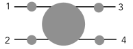
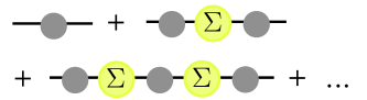
Such diagrams consist of taking the bubble diagrams contributing to the four-point function, represented by Fig. 9(b), and closing two of the external legs:

$$\sum_{p_{2}}\int\frac{d\omega_{2}}{2\pi}L(1,2,1,2)\frac{1}{D_{2}}~{},$$ (B.60)

where we have divided by $D_{2}$ to strip one of the lines we are connecting of the external propagator, see Fig 9(c). The self-energy is simply (B.60) with the incoming and outgoing propagator stripped off,

$$\Sigma_{1}=\frac{1}{D_{1}^{2}}\sum_{p_{2}}\int\frac{d\omega_{2}}{2\pi}L(1,2,1,2)\frac{1}{D_{2}}~{}.$$ (B.61)

Note that the summation over $p_{2}$ gives extra IR divergence $k_{0}^{-\alpha}$. Hence the renormalized propagator is, as is standard, a geometric sum,

$$D_{1}+D_{1}\Sigma D_{1}+D_{1}\Sigma D_{1}\Sigma D_{1}+\ldots=\frac{D_{1}}{1-\Sigma_{1}D_{1}}~{},$$ (B.62)

as shown in Fig. 9(d).

Appendix C Renormalization in quantum field theory

It is instructive to recall how renormalization works in quantum field theory and then compare with our situation. Consider the standard relativistic scalar field theory with a quartic interaction in four spacetime dimensions, see e.g. [36],

$$\mathcal{L}=\frac{1}{2}(\partial\phi)^{2}-\frac{\lambda}{4!}\phi^{4}~{}.$$ (C.1)

Let us consider the fourth cumulant. At tree-level it is $\lambda$. The $\lambda^{2}$-correction to it, given by the one-loop bubble diagram, is UV divergent,

$$\lambda^{2}\int d^{4}q\frac{1}{q^{2}}\frac{1}{(p{-}q)^{2}}\sim\lambda\mathcal{L}(p)/3~{},\ \ \ \ \ \mathcal{L}(p)\equiv-\frac{3\lambda}{32\pi^{2}}\log\left(\frac{\Lambda^{2}}{p^{2}}\right)~{},\ \ \ \ \ \ p\equiv p_{1}+p_{2}~{},$$ (C.2)

where $\Lambda$ is the UV cutoff and we have computed the $s$-channel diagram. This indicates that one needs to sum some class of diagrams. The two-bubble diagram is simply $\lambda\mathcal{L}^{2}$. Summing this (leading log) UV divergent part of all bubble diagrams (and including also the $t$ and $u$ channels, with all external momenta of order $p$), gives,

$$\lambda\sum_{n=0}^{\infty}\mathcal{L}(p)^{n}=\frac{\lambda}{1-\mathcal{L}(p)}~{}.$$ (C.3)

This is now UV-finite.

The point, of course, is that the expansion parameter is not $\lambda$, but $\mathcal{L}(p)$, which is momentum dependent. The one-loop diagram, which for $\lambda\ll 1$ would naively appear to be small, can in fact be large if $\frac{\Lambda^{2}}{p^{2}}$ is sufficiently large. The sum of the bubble diagrams (C.3) now encodes the fourth cumulant at any momentum $p$, though still to order $\lambda^{2}$. Instead of having to perform this sum of leading log divergences of the bubble diagrams each time, it is convenient to take an effective Lagrangian, with quartic coupling $\lambda_{\text{eff}}(p)\phi^{4}$, where one defines the effective coupling to be

$$\lambda_{\text{eff}}(p)=\frac{\lambda}{1-\mathcal{L}(p)}~{}.$$ (C.4)

One says that the coupling runs; that it is momentum dependent. An equivalent way of finding $\lambda_{\text{eff}}(p)$ would have been to compute the beta function from the one-loop diagram,

$$\frac{d\lambda_{\text{eff}}}{d\log(p^{2}/\Lambda^{2})}=\frac{3\lambda_{\text{eff}}^{2}}{32\pi^{2}}~{},$$ (C.5)

and to then integrate to obtain (C.4).

Comparing to our theory describing the kinetics of waves, the loop integral $\mathcal{L}$ appearing here is of course analogous to the loop integral $\mathcal{L}_{1}$ that we had there. What is different in our case of wave kinetics is that generally the wave coupling is a function of the momenta, and more importantly, the presence of the occupation number $n_{k}$ (which decays with $k$) turns the loop integral from being UV divergent to IR divergent.

References

- [1] N. Bogolyubov, “Kinetic equations”, Zh. Eksper. Teoret. Fiz. 16 (1946), 691-702; Acad. Sci. USSR J. Phys. 10 (1946), 265-274.
- [2] J. R. Dorfman, H.v. Beijeren, T. R. Kirkpatrick, Contemporary Kinetic Theory (Cambridge Univ Press 2021).
- [3] R. Peierls, Surprises in Theoretical Physics (Princeton Univ Press 1979).
- [4] J. Dorfman and E. Cohen, “Velocity Correlation Functions in Two and Three Dimensions”, Phys. Rev. Lett. 25, 1257 (1970).
- [5] J. Dorfman and E. Cohen, “Difficulties in the Kinetic Theory of Dense Gases”, J. Math. Phys. 8, 282 (1967).
- [6] K. Kawasaki and I. Oppenheim, “Logarithmic terms in the density expansion of transport coefficients”, Phys. Rev., 139, 1763, 1965
- [7] V. Zakharov, V. Lvov and G. Falkovich, Kolmogorov spectra of turbulence (Springer Berlin 1991).
- [8] V. Rosenhaus and M. Smolkin,“Feynman rules for forced wave turbulence,” JHEP 01, 142 (2023), arXiv:2203.08168 [cond-mat.stat-mech].
- [9] H. W. Wyld, Ann. Phys., 14, 143 (1961).
- [10] V. E. Zakharov and V. S. L’vov, Statistical description of nonlinear wave fields,
- [11] V. Rosenhaus and M. Smolkin,“Wave turbulence and the kinetic equation beyond leading order,” arXiv:2212.02555 [cond-mat.stat-mech].
- [12] T. Buckmaster, P. Germain, Z. Hani, J. Shatah, “Onset of the wave turbulence description of the longtime behavior of the nonlinear Schrödinger equation,” Invent. Math. (2021), arXiv:1907.03667 .
- [13] Y. Deng, Z. Hani, “Full derivation of the wave kinetic equation.”, Invent. math. (2023), arXiv:2104.11204 [math-ap] .
- [14] A. Dymov and S. Kuksin, “Formal Expansions in Stochastic Model for Wave Turbulence 2: Method of Diagram Decomposition,” Journal of Statistical Physics 190:3 (2023), arXiv:1907.02279 [math-phys] .
- [15] A. Kats, V. Kontorovich, “Anisotropic turbulent distributions for waves with a nondecay dispersion law,” Sov Phys JETP 38, 102 (1974).
- [16] S. Nazarenko, Wave Turbulence (Springer, New York 2011).
- [17] O.M. Phillips,“The equilibrium range in the spectrum of wind-generated waves”, J. Fluid Mech. 4, 426 (1958).
- [18] P. Goldreich, and S. Sridhar, “Toward a theory of interstellar turbulence. 2: Strong Alfvenic turbulence,” Astrophys. J. 438, 763-775 (1995).
- [19] A. C. Newell, V. E. Zakharov, “The role of the generalized Phillips’ spectrum in wave turbulence”, Physics Letters A, 372, 4230-4233 (2008)
- [20] S. V. Nazarenko, A. A. Schekochihin J. Fluid Mech., “Critical balance in magnetohydrodynamic, rotating and stratified turbulence: towards a universal scaling conjecture”, vol. 677 pp. 134-153. (2011).
- [21] S. Galtier and S. Nazarenko, “Turbulence of Weak Gravitational Waves in the Early Universe”, Phys. Rev. Lett. 119, 221101 (2017).
- [22] G. Falkovich and K. R. Sreenivasan,“ Lessons from hydrodynamic turbulence”. Physics Today 59(4) : 43 (2006).
- [23] G. Falkovich, Fluid Mechanics (Cambridge Univ Press, 2018).
- [24] G. E. Falkovich and I. V. Ryzhenkova, “Kolmogorov spectra of Langmuir and optical turbulence”, Physics of Fluids B 4, 594 (1992).
- [25] V. S. Lutovinov and V. R. Chechetkin, Zh. Eksp. Teor. Fiz. 76, 223 (1979) [Sov. Phys. JETP 49, 114 (1979)].
- [26] K. Fujimoto1 and M. Tsubota, “Direct and inverse cascades of spin-wave turbulence in spin-1 ferromagnetic spinor Bose-Einstein condensates”, Phys. Rev. A 93, 033620 (2016).
- [27] A. Kats, V. Kontorovich, S. Moiseev and V. Novikov, “Exact power-law solutions of the particle kinetic equations,” Sov Phys JETP 44, 93 (1976).
- [28] G. Falkovich, Y. Kadish, and N. Vladimirova, “Multimode correlations and the entropy of turbulence in shell models”, Phys. Rev. E 108, 015103 (2023), arXiv:2209.05816 [nlin.CD].
- [29] G. Falkovich and N. Vladimirova, “Cascades in nonlocal turbulence”, Phys. Rev. E 91, 041201(R) (2015).
- [30] G. Falkovich, K Gawedzki and M Vergasola, “Particles and fields in fluid turbulence,” Rev. Mod. Phys. 73, 913 (2001).
- [31] J. Polchinski, “Effective Field Theory and the Fermi Surface”, hep-th/9210046.
- [32] D. J. Gross and A. Neveu, “Dynamical Symmetry Breaking in Asymptotically Free Field Theories,” Phys. Rev. D 10, 3235 (1974) doi:10.1103/PhysRevD.10.3235
- [33] , R. Feynman, “Statistical Mechanics: A Set Of Lectures”, (CRC Press, 1988).
- [34] , M. Gell-Mann and K. A. Brueckner,“Correlation Energy of an Electron Gas at High Density,” Phys. Rev. 106, 364-368 (1957) doi:10.1103/PhysRev.106.364.
- [35] V. Rosenhaus, D. Schubring, M. S. J. Shuvo, and M. Smolkin, “Loop diagrams in the kinetic theory of waves”, arXiv:2308.00740 [hep-th].
- [36] M. Peskin and D. V. Schroder, An Introduction to Quantum Field Theory, Westview Press (1995).