On the positivity of $\overline{\rm{MS}}$ parton distributions

We revisit our argument that shows that parton distribution Functions (PDFs) in the $\overline{\rm{MS}}$ scheme are non-negative in the perturbative region, with the main goals of elucidating its domain of validity and clarifying its theoretical underpinnings. We specifically discuss recent results proving that PDFs can turn negative at sufficiently low scale, we clarify quantitatively various aspects of our derivation of positivity in the perturbative region, and we provide an estimate for the scale above which PDF positivity holds.

1 PDF positivity

The issue of positivity of parton distributions raises interesting questions both from a theoretical and a phenomenological point of view. Leading-order (LO) parton distributions are necessarily positive because they are proportional to physically observable cross-sections, while beyond LO positivity depends on the choice of factorization scheme. Hence, PDF positivity goes to the heart of factorization; furthermore, PDF positivity in the commonly used $\overline{\rm{MS}}$ factorization scheme is phenomenologically relevant for PDF determination.

In Ref. [1] we have provided arguments for positivity of PDFs in the $\overline{\rm{MS}}$ factorization scheme, based on starting with a scheme in which PDFs are positive, and then showing that positivity is preserved when transforming to $\overline{\rm{MS}}$, if the scheme change is perturbative, namely in a region in which next-to-leading order (NLO) corrections are smaller than LO terms. Specifically, as candidate starting positive schemes we considered two possibilities: a scheme in which partonic cross-sections are positive beyond LO, and a physical scheme in which PDFs are identified with physical observables. In the former scheme, positivity holds provided the $d$-dimensional PDF is positive before collinear subtraction. In the latter scheme positivity is guaranteed at all scale by that of the physical observable.

These two arguments were argued in Ref. [1] to be equivalent. However, while positivity of the physical observable is guaranteed at all scales, it has been recently shown in Ref. [2] that positivity of the $d$-dimensional collinear-unsubtracted (called “bare” PDF in Ref. [1]) cannot hold at all scales, and must necessarily fail at a low-enough scale. This then raises the issue of the relation between the two routes to positivity of Ref. [1], and more in general, the question of whether the argument of Ref. [2] invalidates the positivity argument of Ref. [1], or perhaps it restricts its domain of validity. This, in turn, raises the question of the precise domain of validity of positivity: as mentioned, in Ref. [1] it was shown to hold in the perturbative region, but no precise assessment of this region was given.

It is the purpose of this note to address all these questions in turn. The argument of Ref. [1] is based on two steps, first the construction or choice of a positive factorization scheme, and then the transformation from this scheme to $\overline{\rm{MS}}$, and consequently a general assessment requires revisiting both steps. Specifically, in Section 2 we address the issue of the implications of the argument of Ref. [2] for PDF positivity, by examining the implications of this argument for the construction of a scheme with positive partonic cross-sections of Ref. [1]. In Section 3 we then study specifically the issue of the transformation to the $\overline{\rm{MS}}$ scheme, by starting with the simplest option, namely, a physical factorization scheme. Finally, in Section 4, by combining the results of the previous two sections, we discuss the relation between the two routes to positivity of Ref. [1] and we assess phenomenologically the domain of applicability of positivity conditions.

2 Factorization: bare and renormalized PDFs

The first route to proving positivity in the $\overline{\rm{MS}}$ scheme considered in Ref. [1] is to construct a factorization scheme in which PDFs are positive, by a suitable modification of the $\overline{\rm{MS}}$ collinear subtraction. This construction is rooted in the $\overline{\rm{MS}}$ factorization of collinear singularities, most easily formulated for deep-inelastic scattering in which case it can be derived from the Wilson expansion. We now summarize this factorization argument; in particular we make explicit and general the dependence on the various scales, for which in Ref. [1] implicit choices were made. The factorization consists of writing deep-inelastic scattering (DIS) structure functions as

$$\frac{1}{x}F(x,Q^{2},\epsilon) =\sum_{j}e^{2}_{j}C_{j}\left(\alpha_{s}(\mu_{r}),\frac{Q^{2}}{\mu_{r}^{2}}\right)\otimes f_{j}(\mu_{r}^{2})$$ (1)

$$=\sum_{j}e^{2}_{j}C_{j}^{R}\left(\alpha_{s}(\mu_{r}),\frac{Q^{2}}{\mu_{f}^{2}}\right)\otimes f_{j}^{R}(\mu_{f}^{2}),$$ (2)

where the coefficient functions $C$ (or partonic cross-sections) are the partonic structure functions computed on external on-shell partons, with all parton masses set to zero, $f_{i}$ is the PDF for the $i$-th parton and $\otimes$ denotes convolution, i.e. $[f\otimes g](x)=\int_{x}^{1}\frac{dy}{y}f(x/y)g(y)$, and for simplicity we are considering the case of photon-induced DIS. Equations (1-2) are written in $d=4-2\epsilon$ dimensions in order to regulate singularities, to be discussed shortly, but in the final factorized formula Eq. (2) the $\epsilon\to 0$ limit can be taken and the coefficient functions and PDFs remain finite. Equations. (1-2) are the leading-order of a Wilson expansion, and thus they only hold up to higher twist corrections, that would involve multiparton operators.

In Eq. (1) $\mu_{r}$ is a renormalization point at which ultraviolet singularities (UV) are subtracted and the PDF $f_{j}(\mu^{2}_{r})$ is defined by a suitable UV renormalization condition, while the coefficient functions $C_{j}$ are affected by collinear singularities. These coefficient functions and PDF were referred to as “bare” in Ref. [1] in order to indicate that factorization of collinear singularities has not been performed yet. However, as stressed in Ref. [2], the composite operator whose matrix element defines the PDF has already undergone UV renormalization, so $f_{j}(\mu^{2}_{r})$ is a UV-renormalized quantity: indeed, the dependence of $\mu_{r}$ arises as a consequence of this UV renormalization. In Eq. (2) instead, $\mu_{f}$ is a factorization scale and the collinear singularities that arise in the massless coefficient functions have been factored in the PDF $f_{j}^{R}$, such that the coefficient function and PDF are separately finite.

In order to understand better the singularity structure of the factorization formulae Eqs. (1-2), we discuss the scale dependence in somewhat greater detail. If factorization is derived from the Wilson expansion, the coefficient functions in Eq. (1) are the inverse Mellin transform of Wilson coefficients. Because of their universality, these can be evaluated by replacing the proton target with a target in which operator matrix elements are known. If one specifically picks a massless, on-shell quark or gluon target, then the coefficient function simply coincides with the structure function for a free on-shell quark or gluon in the massless case. As stressed in Ref. [2], this way of defining the coefficient function (or Wilson coefficient) entails the choice of a specific renormalization condition for the PDF, namely the condition

$$f_{j/i}(z,\mu_{r}^{2})=\delta_{ij}\delta(1-z)\,,$$ (3)

where $f_{j/i}(z,\mu_{r}^{2})$ is the PDF for a $j$-parton in a $i$-parton target, evaluated on-shell and with massless partons. This condition implies that indeed the coefficient function Eq. (1) is just the structure function of a free on-shell massless quark, as computed in Ref. [1], and it corresponds to a specific choice of renormalization scheme, referred to as BPHZ’ in Ref. [2]. The renormalization condition Eq. (3) makes the factorization Eqs. (1)-(2), on which Ref. [1] is based on and denoted as track-B in Ref. [2], consistent with the treatment of factorization given in Refs. [3, 4], denoted as track-A [2].

Because the coefficient function $C_{j}$ in Eq. (1) is evaluated for massless, on-shell quarks, it is affected by collinear singularities. On the other hand, if the structure function is computed in a hadron target it must be finite. This then implies that the PDF $f_{j}(\mu_{r}^{2})$ in Eq. (1) must also be divergent in four dimensions in the BPHZ’ scheme when evaluated for a hadron target so as to cancel the divergence of the coefficient function. Clearly this is a generic property whenever one chooses a target such that the structure function is finite.

In order to understand the divergence of the PDF, and the way it determines its positivity properties, thereby making contact with the argument of Ref. [2], we compute the PDF of a quark in a free off-shell quark target at NLO in the massless case. Combined with the (universal) coefficient function, this amount to the perturbative computation of the structure function of an off-shell quark, which is finite because of the off-shellness of the target. The computation is thus akin to that of an operator matrix element in a free quark state, but now with the off-shellness taking care of the collinear singularity.

This PDF can be thought of as the “perturbative component” of the proton PDF, by interpreting the off-shell target as the internal line of a diagram that contributes to the structure function in a hadron target. The computation is closely related to that of Sec. 8 of Ref. [2], also presented in Ref. [5], which is however performed in scalar Yukawa theory, while here we wish to illustrate the point raised in [2] while remaining in the context of QCD.

We thus consider

$$\frac{1}{x}F^{M_{q}}(x,Q^{2})=e^{2}_{q}C_{q}\left(\alpha_{s}(\mu_{r}),\frac{Q^{2}}{\mu_{r}^{2}}\right)\otimes f^{M}_{q/q}\left(\mu_{r}^{2}\right)+\mathcal{O}(\alpha_{s}^{2})$$ (4)

where $p^{2}=M^{2}$ is the target quark virtuality and $f^{M}_{q/q}$ is the PDF for a quark in a quark target with electric charge $e_{q}$, and henceforth all quantities will be determined up to NLO, i.e. neglecting terms that lead to $\mathcal{O}(\alpha_{s}^{2})$ contributions to the structure function. The notation $F^{M_{q}}$ indicates that this is the structure function of a free off-shell quark. Note that up to $O(\alpha_{s}^{2})$ only diagonal contributions, i.e. such as the struck quark is the same flavor as the target quark, are present, but starting at $O(\alpha_{s}^{2})$ the PDF $f^{M}_{q_{i}/q_{j}}$ for any quark of flavor $i$ in a target $j$-quark is nonvanishing so the structure function has again the form of Eq. (4) with a sum over quark flavors $j$.

The coefficient function $C_{q}$ was given in Ref. [1], Eq. (2.24): it is universal, hence the same regardless of whether the target is a quark or indeed a hadron. Because the target is off-shell the PDF $f^{M}_{q/q}$ can only satisfy the condition Eq. (3) at LO: indeed, as already mentioned, beyond LO $f^{M}_{q/q}$ must necessarily contain a collinear singular contributions that cancels against that of the coefficient function, leading to a finite structure function. In order to compute it at NLO, and check the cancellation of the collinear singularity, we start with a “fully bare” PDF $f^{M,\,0}_{q/q}$, and perform UV renormalization in the BPHZ’ scheme. This then gives the PDF $f^{M}_{q/q}$ of Eq. (4), corresponding to $f_{j}(\mu_{r}^{2})$ of Eq. (1): UV renormalized, but not yet collinear factorized, and called “bare” in Ref. [1]. From this PDF the “fully renormalized” PDF $f^{M,\,R}_{q/q}$, to be defined precisely below, and corresponding to $f_{j}^{R}(\mu_{f}^{2})$ of Eq. (2), is derived through collinear factorization. We will henceforth stick to the terminology “fully bare” and “fully renormalized” in order to refer to $f^{M,\,0}_{q/q}$ and $f^{M,\,R}_{q/q}$ respectively. The singularity structure that we expect, and that we will verify explicitly, is the following: the fully bare PDF $f^{M,\,0}_{q/q}$, is UV divergent and IR finite; after UV renormalization, the PDF $f^{M}_{q/q}$ is UV finite but collinear divergent; the fully renormalized PDF $f^{M,\,R}_{q/q}$ is finite. The real emission contribution to the coefficient function $C_{q}$ is of course UV finite at NLO, it is IR finite after addition of the virtual correction but it remains collinear singular; its collinear singularity cancels against that of the PDF $f^{M}_{q/q}$ in Eq. (4).

The NLO correction to the PDF $f^{M}_{q/q}$ involves [4] an integration over the momentum of the gluon radiated from the quark line, in which the longitudinal and transverse momentum integrations are treated asymmetrically, because the off-shell quark whose PDFs is being determined has a well-defined value of the longitudinal momentum, which corresponds to that specified by the renormalization condition Eq. (3) that enforces it to all orders. The integral over the transverse momentum ${\bf k}_{\text{T}}$ of the emitted quark then leads to the result

$$f^{M,\,0}_{q/q}\left(x,\mu^{2},\epsilon\right)=\delta\left(1-x\right)+\frac{\alpha_{s}\left(\mu\right)}{2\pi}C_{F}\left\{\left[\Gamma\left(\epsilon\right)\left(\frac{\Delta^{2}\left(x\right)}{4\pi\mu^{2}}\right)^{-\epsilon}p_{qq}\left(x\right)\right]_{+}+f_{f}(x)\right\}.$$ (5)

which holds in $d$ dimensions and is UV divergent as $\epsilon\to 0$ (see Appendix A for the details of the calculation). In Eq. (5) $\mu$ is the standard dimensional regularization scale; $p_{qq}(x)$ is implicitly defined in terms of the quark-quark splitting function $P_{qq}(x)$ as $P_{qq}(x)=C_{F}\left[p_{qq}(x)\right]_{+}$; $\Delta^{2}\left(x\right)$ is given by

$$\Delta^{2}\left(x\right)=-x\left(1-x\right)M^{2}\,;$$ (6)

and $f_{f}(x)$ is a UV finite and thus scale-independent contribution, whose explicit form is given in Appendix A, Eq. (47).

The UV divergence of the fully bare PDF Eq. (5) is a consequence of the fact that the PDF is defined as the matrix element of a composite operator [6]. The divergence can be removed by a subtraction

$$f^{M}_{q/q}\left(x,\mu_{r}^{2},\epsilon\right)=f^{M,\,0}_{q/q}\left(x,\mu_{r}^{2},\epsilon\right)-\delta^{\rm UV}\left(x,\mu_{r}^{2},\epsilon\right),$$ (7)

thereby leading to the UV renormalized, but still collinear divergent PDF $f^{M}_{q/q}$. The UV counterterm in Eq. (7) is fixed by the renormalization condition Eq. (3), i.e. by considering Eq. (5) in the on-shell, massless case and subtracting everything but the $\delta(1-x)$ contribution to its r.h.s., with $\mu=\mu_{r}$. The explicit expression of $\delta^{\rm UV}$ is found performing the computation leading to Eq. (5) in the on-shell, massless case, i.e. starting from the expression of the bare PDF in terms of transverse momentum integrals (see Appendix A, Eq. (A)) and setting $M^{2}=0$. This leads to

$$\delta^{\rm UV}\left(x,\mu_{r}^{2},\epsilon\right)=\frac{\alpha_{s}\left(\mu_{r}\right)}{2\pi} P_{qq}\left(x\right)\,4\pi\mu_{r}^{2\epsilon}\int\frac{d^{2-2\epsilon}{\bf k}_{\text{T}}}{\left(2\pi\right)^{2-2\epsilon}}\frac{1}{k_{\text{T}}^{2}}\,.$$ (8)

It is useful to separate the UV and IR regions of integration over ${\bf{k}}_{\text{T}}$ in Eq. (8); this can be done by introducing an auxiliary mass parameter on which nothing depends, and which we may well take equal to the virtuality $M$, through the identity

$$4\pi\mu_{r}^{2\epsilon}\int\frac{d^{2-2\epsilon}\bf{k}_{\text{T}}}{\left(2\pi\right)^{2-2\epsilon}}\frac{1}{k_{\text{T}}^{2}} =4\pi\mu_{r}^{2\epsilon}\int\frac{d^{2-2\epsilon}\bf{k}_{\text{T}}}{\left(2\pi\right)^{2-2\epsilon}}\frac{1}{k_{\text{T}}^{2}+M^{2}}+4\pi\mu_{r}^{2\epsilon}\int\frac{d^{2-2\epsilon}\bf{k}_{\text{T}}}{\left(2\pi\right)^{2-2\epsilon}}\frac{M^{2}}{k_{\text{T}}^{2}\left(k_{\text{T}}^{2}+M^{2}\right)}$$

$$=\left(\frac{M^{2}}{4\pi\mu_{r}^{2}}\right)^{-\epsilon}\Gamma\left(\epsilon\right)-\left(\frac{M^{2}}{4\pi\mu_{r}^{2}}\right)^{-\epsilon}\Gamma\left(\epsilon\right).$$ (9)

Note that the first integral (UV divergent) converges in the $\epsilon>0$ region, while the second one (IR divergent) converges when $\epsilon<0$.

We thus get that the PDF at scale $\mu_{r}$ is given by

$$f^{M}_{q/q} \left(x,\mu_{r}^{2},\epsilon\right)=\delta\left(1-x\right)+\frac{\alpha_{s}\left(\mu_{r}\right)}{2\pi}C_{F}\left\{\left[\Gamma\left(\epsilon\right)\left(\frac{\Delta^{2}\left(x\right)}{4\pi\mu_{r}^{2}}\right)^{-\epsilon}p_{qq}\left(x\right)\right]_{+}+f_{f}(x)\right\}$$

$$=\delta\left(1-x\right)+\frac{\alpha_{s}\left(\mu_{r}\right)}{2\pi}P_{qq}\left(x\right)\left(\frac{1}{\epsilon}-\gamma_{E}\right)+C_{F}\left\{\left[\ln\frac{\mu_{r}^{2}}{|\Delta^{2}\left(x\right)|}p_{qq}\left(x\right)\right]_{+}+\bar{f}_{f}(x)\right\},$$ (10)

where $\bar{f}_{f}(x)=f_{f}(x)+i\arg(-M^{2})$ now includes an imaginary contribution when $M^{2}>0$ so the off-shell quark can decay into a quark-gluon pair. Note the different nature of the poles appearing in Eqs. (5) and (2): the UV divergence in Eq. (5) has been canceled by the UV divergent integral of Eq. (2), but the PDF has now acquired a collinear divergence, which is the pole appearing in Eq. (2).

We can finally determine the fully renormalized PDF. In Ref. [1] the collinear counterterm that removes the singularity from both the coefficient function and PDF was determined by performing an $\overline{\rm{MS}}$ subtraction of the coefficient function. Here we can easily determine it from the expression of the PDF Eq. (2), by writing the fully renormalized PDF as

$$f^{M,\,R}_{q/q}\left(x,\mu_{f}^{2}\right)=\lim_{\epsilon\to 0}\left[f^{M}_{q/q}\left(x,\mu_{r}^{2},\epsilon\right)+\delta^{{\overline{\rm{MS}}}}_{q}\left(x,\frac{\mu_{f}^{2}}{\mu^{2}_{r}},\epsilon\right)\right],$$ (11)

where we have adopted the same sign convention for the counterterm as in Ref. [1]. It immediately follows that the $\overline{\rm{MS}}$ counterterm is

$$\delta^{{\overline{\rm{MS}}}}_{q}\left(x,\frac{\mu_{f}^{2}}{\mu^{2}_{r}},\epsilon\right)=\frac{\alpha_{s}\left(\mu_{r}\right)}{2\pi}\left(\frac{\mu_{f}^{2}}{4\pi\mu^{2}_{r}}\right)^{-\epsilon}\left(-\frac{1}{\epsilon}+\gamma_{E}\right)P_{qq}(x)\,,$$ (12)

and the fully renormalized PDF is

$$f^{M,\,R}_{q/q}\left(x,\mu_{f}^{2}\right) =\delta\left(1-x\right)+\frac{\alpha_{s}\left(\mu_{r}\right)}{2\pi}C_{F}\left\{\left[\ln\frac{\mu_{f}^{2}}{|\Delta^{2}\left(x\right)|}p_{qq}\left(x\right)\right]_{+}+\bar{f}_{f}(x)\right\}.$$ (13)

Using the expression of the NLO coefficient function from Ref. [1] it is easy to check that the counterterm also removes the collinear divergence from the coefficient function. The renormalized coefficient function is

$$C^{R}_{q} \left(x,\frac{Q^{2}}{\mu_{f}^{2}}\right)=\lim_{\epsilon\to 0}C_{q}\left(x,\left(\frac{Q^{2}}{\mu_{r}^{2}}\right),\epsilon\right)-\delta^{{\overline{\rm{MS}}}}_{q}\left(x,\frac{\mu_{f}^{2}}{\mu^{2}_{r}},\epsilon\right)$$

$$=\delta(1-x)+\frac{\alpha_{s}\left(\mu_{r}\right)}{2\pi}\left\{P_{qq}(x)\ln\frac{Q^{2}}{\mu^{2}_{f}}+\left[C_{F}p_{qq}(x)\ln\left(\frac{1-x}{x}\right)\right]_{+}+D(x)\right\},$$ (14)

with

$$D(x)=C_{F}\left[-\frac{3}{2}{\left(\frac{1}{1-x}\right)_{+}}+3+2x-4\delta(1-x)\right]\,.$$ (15)

The expression of the renormalized coefficient function of Ref. [1] coincides with Eq. (2) with the choice $\mu^{2}_{f}=\mu_{r}^{2}=Q^{2}$.

The dependence of the PDF Eq. (2) on the scale $\mu_{r}$, and consequently of the fully renormalized PDF Eq. (13) on the scale $\mu_{f}$, is driven by the splitting function $P_{qq}$ as it should: the collinear singularity in the coefficient function exactly matches the UV anomalous dimension of the operator matrix element, i.e. of the PDF, in such a way that the singularities in the coefficient function and PDF in Eq. (1) cancel each other. Indeed, up to the finite terms, we could have obtained Eq. (2) by simply noting that (a) the dependence of the PDF $f^{M}_{q/q}\left(x,\mu_{r}^{2},\epsilon\right)$ on the scale $\mu_{r}$ must satisfy the QCD evolution equation, i.e. a Callan-Symanzik equation with anomalous dimension $P_{qq}$ (more precisely, its Mellin transform); (b) the dependence on $\mu_{r}$ must cancel between the coefficient function and the PDF; (c) the dependence on scale of the coefficient function is due to its collinear singularity; (d) the PDF depends (on top of the renormalization scale) on a scale $\Delta^{2}$ that cuts off the collinear singularity. The computation that we presented amounts to an explicit check of all this.

We now turn to the positivity properties of the PDF. As a preliminary observation we note that the PDF of a quark is actually a distribution, so we only discuss its positivity properties in the $x<1$ region. Also, if $M^{2}>0$ the PDF develops an absorptive part, in which case when discussing positivity we refer to the positivity of the real part of the PDF. Also, we recall that our whole argument starts with the leading-twist factorization Eqs. (1-2), hence at low enough scale any conclusion is not only subject to large higher order perturbative corrections, but also to sizable higher-twist corrections. All this said, we note that before collinear subtraction the PDF $f^{M}_{q/q}$ Eq. (2) contains a singular contribution proportional to $\frac{P_{qq}\left(x\right)}{\epsilon}$, and associate logarithmic contribution proportional to $P_{qq}\ln\frac{\mu_{r}^{2}}{|\Delta^{2}\left(x\right)|}$. But for $x<0$, $P_{qq}(x)>0$, so the logarithmic term is negative at low enough scale $\mu_{r}^{2}<|\Delta^{2}|$, and the PDF becomes negative at low enough $\mu_{r}^{2}$ for any fixed value of $\epsilon<0$, in the region of convergence of the transverse momentum integral. Correspondingly for any fixed value of $\mu_{r}^{2}$ the PDF becomes negative for sufficiently small $\epsilon$. The interplay of $\epsilon$ and $\mu_{r}^{2}$ in the positivity condition is of course due to the fact that in dimensional regularization with $\overline{\rm{MS}}$ subtraction $\mu=\mu_{r}$ plays the role of a cutoff. The fact that the PDF $f^{M}_{q/q}$ is negative at low scale is the main observation of Ref. [2].

Turning now to the fully renormalized PDF $f^{M,\,R}_{q/q}\left(x,\mu_{f}^{2}\right)$ Eq. (13), it is clear that, since the logarithmic contribution is the same as before collinear subtraction, but with now $\mu_{r}$ replaced by $\mu_{f}$, by the same argument this contribution will be dominant and the PDF will always be positive for large enough $\mu_{f}$. Conversely, $f^{M,\,R}_{q/q}\left(x,\mu_{f}^{2}\right)$ will always be negative for small enough $\mu_{f}$, though of course at low scale both the NLO perturbative approximation, and in fact the whole leading-twist approach on which the computation is based fail. The transition between these two regions depends on the finite terms, as also emphasized in Sec. 8 of Ref. [2] (see in particular Fig. 2), where this result is discussed in the case of a Yukawa theory.

Hence, positivity of the fully renormalized PDF will surely hold only at high enough scale, such that $\mu_{f}$ is an UV scale, as it should be. In a hadronic target the PDF cannot be computed explicitly, however the same calculation leading to Eq. (13) can be used to obtain the perturbative dependence of the PDF on the factorization scale. It is the clear that the same arguments apply, but now with $\Delta^{2}\left(x\right)$ replaced by a characteristic scale $\Lambda^{2}_{h}$ of the hadronic target. Namely, the renormalized quark PDF in a hadron target $f^{R}_{q}$ contains a logarithmic contribution of the form of Eq. (13), i.e. it is given by

$$f^{R}_{q}\left(x,\mu_{f}^{2}\right)=\delta(1-x)+\frac{\alpha_{s}\left(\mu_{r}\right)}{2\pi}\ln\frac{\mu_{f}^{2}}{\Lambda^{2}_{h}}P_{qq}+f_{h}(x)$$ (16)

where $f_{h}(x)$ is a scale-independent contribution determined by nonperturbative physics, and the scale dependence is fully determined by the QCD evolution equation.

We can now examine the positivity argument of Ref. [1] within the context of this model computation. We start with the observation that combining Eqs. (2) and (13), the structure function $F^{M_{q}}(x,Q^{2})$, Eq. (4) when $\epsilon=0$ and $x<1$, is given by

$$\frac{1}{x}F^{M_{q}}(x,Q^{2}) =e^{2}_{q}\frac{\alpha_{s}\left(\mu_{r}\right)}{2\pi}\left[P_{qq}(x)\ln\frac{Q^{2}(1-x)/x}{|\Delta^{2}\left(x\right)|}+D(x)+C_{F}\bar{f}_{f}(x)\right]$$ (17)

$$=e^{2}_{q}\frac{\alpha_{s}\left(\mu_{r}\right)}{2\pi}C_{F}\left[\left((1+x^{2})\ln\frac{Q^{2}}{|M^{2}|x^{2}}-\frac{3}{2}\right)\frac{1}{1-x}+3x+1\right].$$ (18)

The structure function is positive for all $x$ provided $Q^{2}$ is large enough (the exact condition is $\frac{Q^{2}}{|M^{2}|}>\exp\frac{3}{4}\approx 2$). This follows from the fact that in this simple model the argument of the log is $\frac{Q^{2}(1-x)/x}{|\Delta^{2}\left(x\right)|}=\frac{Q^{2}}{|M|^{2}x^{2}}$.

The argument of Ref. [1] then consists of noting that in standard $\overline{\rm{MS}}$ factorization, in which the coefficient function is given by Eq. (2) with $\mu^{2}_{f}=\kappa Q^{2}$ (or, more in general, $\mu^{2}_{f}$ is taken to be $x$-independent) the coefficient function acquires a spurious logarithmic dependence on $1-x$ because subtraction of the collinear singularity is performed at a fixed $x$-independent scale $Q^{2}$, rather than at the physical scale of the process. This is obvious in the model computation: in $\overline{\rm{MS}}$ factorization the logarithm is split according to

$$\ln\frac{Q^{2}(1-x)/x}{|\Delta^{2}\left(x\right)|}=\ln\frac{1-x}{x}+\ln\frac{Q^{2}}{|M^{2}|x(1-x)}\,,$$ (19)

the first log is included in the coefficient function, and the second in the PDF. This amounts to splitting a positive log into the sum of a negative contribution, included in the coefficient function, and a compensating contribution included in the PDF. Consequently, the NLO contribution to the coefficient function may turn negative, and if the structure function is a measured positive observable from which the PDF is extracted by comparing to the data the $\overline{\rm{MS}}$ prediction, the PDF may then turn out to be negative as well.

In Ref. [1] it was consequently suggested to perform factorization through subtraction at the physical scale, in such a way that the coefficient function remains positive. In such a scheme, the logarithmic contributions that are associated to collinear divergences are split between coefficient function and PDF in a way that preserves the positivity of both. The extra caveat, and main point of Ref. [2], is that this can be only done provided the scale is high enough, because otherwise the $d$-dimensional PDF and the four-dimensional fully renormalized PDF are not positive to begin with, so positivity is violated however one splits the log. This is manifest in the model computation: for $Q^{2}<|M^{2}|$ the logarithmic contribution is negative, for small enough $Q^{2}$ it will overwhelm any positive finite term, and the structure function Eq. (18) may turn negative. Hence even in factorization schemes such as those considered in Ref. [1] positivity of the PDF (and of the perturbative, leading-twist structure function) only holds at high enough scale: physically, at scales which are significantly larger than the hadronic target mass scale $\Lambda_{h}^{2}$ that regulates the collinear singularity.

In summary, the import of the argument of Ref. [2] is that the construction of a scheme in which coefficient functions are positive of Ref. [1] only leads to positive PDFs and positive physical cross-sections at high enough scale. Given that the whole argument applies at leading twist and in the perturbative regime, it is unclear whether this is a further restriction. We will address the issue of the range of validity of positivity in the last section.

3 From a physical scheme to $\overline{\rm{MS}}$

The second step in proving positivity of $\overline{\rm{MS}}$ PDFs is to verify that positivity is preserved when transforming to $\overline{\rm{MS}}$ from the scheme in which PDFs are positive. The argument is streamlined if one starts from a physical scheme, the second option considered in Ref. [1] as an alternative to the scheme discussed in the previous section. In a physical scheme [7, 8, 9, 10, 11], the PDF is defined in terms of a physical observable, by identifying it to all orders with a observable to which it is proportional at leading order, i.e., the Wilson coefficients are set to one to all orders by scheme choice. An example is the “DIS” scheme [7] in which the quark PDFs are identified with DIS structure functions, so that for instance a nonsinglet PDF is defined by

$$\frac{1}{x}F_{2}^{{\rm NS}}(x,Q^{2})=\langle e_{i}^{2}\rangle{f^{{\rm NS},\,\rm DIS}}(x,Q^{2})\,,$$ (20)

where $f^{{\rm NS}}$ is a difference of two quark or antiquark PDFs, $\langle e^{2}_{i}\rangle=\frac{1}{2}\left(e^{2}_{i}+e^{2}_{j}\right)$ is the average of their electric charges, and $F_{2}^{{\rm NS}}$ is the corresponding combination of photon-induced DIS structure functions.

It may seem that a positivity argument in such a scheme is more general than that presented in the previous section, because physical observables are positive by construction, while in the previous section the PDF was defined in terms of leading-twist quantities computed to finite perturbative order, hence subject to the limitations of the perturbative, leading-twist approximation. This greater generality is however fictitious, because it is only in the perturbative leading-twist approximation that PDFs are universal. We will discuss this point further in the next section: here it should be kept in mind that all the subsequent manipulations in this section only hold at leading twist and finite perturbative order.

We thus start by generalizing Eq. (20) in such a way as to define all PDFs in terms of physical observables. Indeed, the difference of structure functions Eq. (20) is not positive, but in a full physical scheme each individual PDF is related to an individual observable and thus separately positive, though for definiteness we start by considering the nonsinglet combination in order to avoid gluon mixing. The generalization of Eq. (20) for a general physical scheme is

$$\sigma(x,Q^{2})=\sigma_{0}f^{\rm PHYS}(x,Q^{2}),$$ (21)

where $\sigma(x,Q^{2})$ is now a vector of physical observables, $f^{\rm PHYS}(x,Q^{2})$ is a vector of PDFs, and $\sigma_{0}$ is a diagonal matrix of coefficients, which accounts for the mismatch in normalization between the physical observable and the PDF, such as the factor $\langle e_{i}^{2}\rangle$ that relates the PDF and the structure function. Equation (21) corresponds in particular to the convenient choice of choosing [10, 1] $\sigma(x,Q^{2})$ as observables that are linear in the PDF, such as deep-inelastic structure functions which at leading order define the quark and a Higgs production process which defines the gluon.

Because in the $\overline{\rm{MS}}$ scheme

$$\frac{1}{x}F_{2}^{{\rm NS}}(x,Q^{2}) =\langle e_{i}^{2}\rangle C^{\rm NS,\,{\overline{\rm{MS}}}}\left(\alpha_{s}(Q^{2})\right)\otimes f^{{\rm NS}\,{\overline{\rm{MS}}}}(Q^{2})$$

$$=\langle e_{i}^{2}\rangle\left[1+\frac{\alpha_{s}}{2\pi}C^{(1),\,\rm NS,\,{\overline{\rm{MS}}}}\otimes+\mathcal{O}(\alpha_{s}^{2})\right]f^{{\rm NS},\,{\overline{\rm{MS}}}}(Q^{2})\,,$$ (22)

it immediately follows that

$${f^{{\rm NS},\,\rm DIS}}(x,Q^{2}) =C^{\rm NS,\,{\overline{\rm{MS}}}}\left(\alpha_{s}(Q^{2})\right)\otimes f^{{\rm NS}\,{\overline{\rm{MS}}}}(Q^{2})$$

$$=\left[1+\frac{\alpha_{s}}{2\pi}C^{(1),\,\rm NS,\,{\overline{\rm{MS}}}}(x)\otimes\right]{f^{{\rm NS},\,{\overline{\rm{MS}}}}}(Q^{2})+\mathcal{O}(\alpha_{s}^{2})\,,$$ (23)

so

$$f^{{\rm NS},\,{\overline{\rm{MS}}}}(x,Q^{2}) =\left[C^{\rm NS,\,{\overline{\rm{MS}}}}\right]^{-1}\left(\alpha_{s}(Q^{2})\right)\otimes f^{{\rm NS},\,\rm DIS}(Q^{2})$$ (24)

$$=\left[1-\frac{\alpha_{s}}{2\pi}C^{(1),\,\rm NS,\,{\overline{\rm{MS}}}}(x)\otimes+\mathcal{O}(\alpha_{s}^{2})\right]f^{{\rm NS},\,\rm DIS}(Q^{2})\,.$$ (25)

Note that in Eq. (24) $\left[C^{\rm NS,\,{\overline{\rm{MS}}}}\right]^{-1}$ denotes the functional inverse of the coefficient function upon convolution, i.e., the distribution (in general) such that

$$\left[C^{\rm NS,\,{\overline{\rm{MS}}}}\otimes\left[C^{\rm NS,\,{\overline{\rm{MS}}}}\right]^{-1}\right](x)=\delta(1-x).$$ (26)

Equation (25) then provides its perturbative expression up to $\mathcal{O}(\alpha_{s})$.

In Ref. [1] it was observed that the coefficient function $C^{(1),\,{\overline{\rm{MS}}}}(x)(\alpha_{s}(Q^{2}))$ is positive for all $x$, which suggests that its inverse is also positive. In order to prove this, it is not sufficient to use the perturbative inversion Eq. (25) because the $\mathcal{O}(\alpha_{s})$ correction is not uniformly small for all $x$, and it is in fact unbounded as $x\to 1$ so the $\mathcal{O}(\alpha_{s})$ truncation is not justified. In Ref. [1] positivity of the inverse was then argued to hold by performing an exact inversion in the $x\to 1$ region and showing that as $x\to 1$ the inverse coefficient function $\left[C^{\rm NS,\,{\overline{\rm{MS}}}}\right]^{-1}$ vanishes. We now revisit this argument, in particular, by explicitly discussing the treatment of distributional contributions.

To this purpose, we write the coefficient function up to $\mathcal{O}(\alpha_{s})$ as follows:

$$C^{\rm NS,\,{\overline{\rm{MS}}}}(x) =\delta(1-x)+\frac{\alpha_{s}}{2\pi}\left[\delta(1-x)\Delta^{(1)}+C_{F}^{(1),\,{\overline{\rm{MS}}}}(x)+C_{D}^{(1),\,{\overline{\rm{MS}}}}(x)\right]+\mathcal{O}(\alpha_{s}^{2})$$ (27)

$$=\left[\delta(1-x)+\frac{\alpha_{s}}{2\pi}\left[\delta(1-x)\Delta^{(1)}+C_{F}^{(1),\,{\overline{\rm{MS}}}}(x)\right]\right]$$

$$\qquad\otimes\left[\delta(1-x)+\frac{\alpha_{s}}{2\pi}C_{D}^{(1),\,{\overline{\rm{MS}}}}(x)\right]+\mathcal{O}(\alpha_{s}^{2}).$$ (28)

In Eq. (27) $C_{F}^{(1),\,{\overline{\rm{MS}}}}(x)$ are contributions such that $\lim_{x\to 1}R_{F}(x)$ is finite, where $R_{F}(x)$ is defined as

$$R_{F}(x)\equiv\frac{[C_{F}^{(1),\,{\overline{\rm{MS}}}}\otimes f](x)}{f(x)},$$ (29)

while $C_{D}^{(1),\,{\overline{\rm{MS}}}}(x)$ are contributions such that, defining

$$R_{D}(x)\equiv\frac{[C_{D}^{(1),\,{\overline{\rm{MS}}}}\otimes f](x)}{f(x)},$$ (30)

then $\lim_{x\to 1}R_{D}(x)=\infty$. Contributions $C_{D}^{(1),\,{\overline{\rm{MS}}}}(x)$ will be henceforth referred to as divergent contributions. As well known, divergent contributions to diagonal coefficient functions are present to all perturbative orders in the $\overline{\rm{MS}}$ scheme: they are proportional to $S_{k}(x)=\left[\frac{\ln^{k}(1-x)}{1-x}\right]_{+}$ and they are due to soft gluon emission [12, 13]. Note that in principle unbounded contributions are also present when $x\to 0$. These could be handled in the same way, but we will not discuss them since PDFs grow large and positive as $x\to 0$ due to high-energy logs [14], so positivity constraints are of no importance.

Clearly, there is some latitude in defining the separation of Eq. (27) of the coefficient function into an $C_{F}^{(1),\,{\overline{\rm{MS}}}}$ term and a $C_{D}^{(1),\,{\overline{\rm{MS}}}}$ term, since we can always subtract a finite contribution from $C_{F}^{(1),\,{\overline{\rm{MS}}}}$ and include it into $C_{D}^{(1),\,{\overline{\rm{MS}}}}$: for example, $\left[\frac{1+x^{2}}{1-x}\right]_{+}=\frac{1+x}{(1-x)_{+}}+\frac{3}{2}\delta(1-x)$. We will define $C_{D}^{(k),\,{\overline{\rm{MS}}}}(x)$ as the contribution that includes all and only the $S_{k}(x)$ terms. With this definition, up to $\mathcal{O}(\alpha_{s})$ we have

$$C_{D}^{(1),\,{\overline{\rm{MS}}}}(x)=C_{F}\left(2\left[\frac{\ln(1-x)}{1-x}\right]_{+}-\frac{3}{2}\left[\frac{1}{1-x}\right]_{+}\right)=2C_{F}\left[\frac{\ln(1-x)}{1-x}\right]_{+}+\hbox{NLL}(1-x).$$ (31)

Having written the coefficient function as in Eq. (3) its inverse can be determined by performing the inversion perturbatively for all terms but $C_{D}^{(1),\,{\overline{\rm{MS}}}}(x)$: namely

$$\left[C^{\rm NS,\,{\overline{\rm{MS}}}}\right]^{-1}= \left[\delta(1-x)-\frac{\alpha_{s}}{2\pi}\left(\delta(1-x)\Delta^{(1)}+C_{F}^{(1),\,{\overline{\rm{MS}}}}(x)\right)\right]$$

$$\qquad\otimes\left[\delta(1-x)+\frac{\alpha_{s}}{2\pi}C_{D}^{(1),\,{\overline{\rm{MS}}}}(x)\right]^{-1}+\mathcal{O}(\alpha_{s}^{2}),$$ (32)

where now $C_{D}^{(1),\,{\overline{\rm{MS}}}}(x)$ must be computed as the exact inverse, Eq. (26).

The exact inverse of the divergent contribution was computed already in Ref. [1] to leading logarithmic accuracy, and it was shown to be finite in the $x\to 1$ limit. This was argued to be in agreement with the expectation that the inverse of a divergent coefficient is actually finite, based on Mellin-space considerations. Namely, the Mellin transform of a divergent coefficient function diverges as the Mellin variable $N\to\infty$, but the Mellin-space inverse is just the reciprocal, so the Mellin transform of the inverse vanishes as $N\to 0$, implying that the inverse is finite.

We wish now to make this argument more explicit by fully working out distributional contributions and explicitly proving their positivity. To leading logarithmic accuracy we have [1]

$$\left[\delta(1-x)+\frac{\alpha_{s}}{2\pi}C_{D}^{(1),\,{\overline{\rm{MS}}}}(x)\right]^{-1}=\delta\left(1-x\right)$$

$$\qquad-2C_{F}\frac{\alpha_{s}}{2\pi}\left(\frac{\ln(1-x)}{\left(1+C_{F}\frac{\alpha_{s}}{2\pi}\ln^{2}(1-x)\right)^{2}}\frac{1}{1-x}\right)_{+}+\hbox{NLL}(1-x).$$ (33)

We can now discuss the positivity of the various contributions by working out their action on a test PDF. Note that when substituting the inverse in Eq. (24) the PDF that is acted upon is guaranteed to be positive, because it is a physical observable. We use the identity

$$\left[f_{+}\otimes g\right]\left(x\right) =\int_{x}^{1}\frac{dz}{z}f\left(z\right)_{+}g\left(\frac{x}{z}\right)$$

$$=\int_{x}^{1}\frac{dz}{z}f\left(z\right)\left[g\left(\frac{x}{z}\right)-zg\left(x\right)\right]-g\left(x\right)\int_{0}^{x}dz\,f\left(z\right)$$ (34)

We get

$$\left[\delta(1-x)+\frac{\alpha_{s}}{2\pi}C_{D}^{\left(1\right),\,{\overline{\rm{MS}}}}\left(x\right)\right]^{-1}\otimes f^{{\rm NS},\,\rm DIS}\left(x\right)=$$

$$= \quad 2C_{F}\frac{\alpha_{s}}{2\pi}\int_{x}^{1}\frac{dz}{z}\frac{\ln\left(\frac{1}{1-z}\right)}{\left(1+C_{F}\frac{\alpha_{s}}{2\pi}\ln^{2}\left(1-z\right)\right)^{2}}\frac{f^{{\rm NS},\,\rm DIS}(\frac{x}{z})-zf^{{\rm NS},\,\rm DIS}\left(x\right)}{1-z}$$

$$\qquad+f^{{\rm NS},\,\rm DIS}\left(x\right)\left[1+2C_{F}\frac{\alpha_{s}}{2\pi}\int_{0}^{x}\frac{dz}{1-z}\frac{\ln\left(1-z\right)}{\left(1+C_{F}\frac{\alpha_{s}}{2\pi}\ln^{2}\left(1-z\right)\right)^{2}}\right]$$ (35)

$$= \quad 2C_{F}\frac{\alpha_{s}}{2\pi}\int_{x}^{1}\frac{dz}{z}\frac{\ln\left(\frac{1}{1-z}\right)}{\left(1+C_{F}\frac{\alpha_{s}}{2\pi}\ln^{2}(1-z)\right)^{2}}\frac{f^{{\rm NS},\,\rm DIS}\left(\frac{x}{z}\right)-zf^{{\rm NS},\,\rm DIS}(x)}{1-z}$$

$$\qquad+f^{{\rm NS},\,\rm DIS}\left(x\right)\left[1+C_{F}\frac{\alpha_{s}}{2\pi}\frac{\ln^{2}\left(1-x\right)}{1+C_{F}\frac{\alpha_{s}}{2\pi}\ln^{2}(1-x)}\right].$$ (36)

Firstly, it is clear that, as argued in Ref. [1], both contributions on the r.h.s. of Eq. (3) are bounded as $x\to 1$: the integral vanishes because the integrand is regular and the range of integration shrinks to zero, and the remaining contribution in the $x\to 1$ limit is proportional to $f^{{\rm NS},\,\rm DIS}\left(x\right)$.

Furthermore, it is also clear that both contributions are positive. The integral is positive because at large $x\gtrsim 0.5$ (where the contribution that we are looking at becomes unbounded) $f^{{\rm NS},\,\rm DIS}(x)$ is a decreasing function of its argument, and all other terms in the integrand are positive. The contribution proportional to $f^{{\rm NS},\,\rm DIS}(x)$ is manifestly positive because the coefficient is manifestly positive, and $f^{{\rm NS},\,\rm DIS}(x)$ also is.

The argument is then easily generalized to include quark-gluon mixing and thus the singlet contribution, i.e. to the general case of Eq. (21). In such case, Eq. (3) becomes

$$f^{\rm DIS}(x,Q^{2})=C^{{\overline{\rm{MS}}}}\left(\alpha_{s}(Q^{2})\right)\otimes f^{{\overline{\rm{MS}}}}(Q^{2}),$$ (37)

where now $C^{{\overline{\rm{MS}}}}$ is a matrix of coefficient functions for the set of processes that have been chosen to define the physical scheme.

The rest of the argument is then essentially unchanged, due to the fact that, as already noted in Ref. [1], as $x\to 1$ the matrix of coefficients $C^{{\overline{\rm{MS}}}}(x)$ becomes diagonal. Indeed, Eq. (27) still holds, with now $C_{D}^{(1),\,{\overline{\rm{MS}}}}(x)$ a diagonal matrix as only the diagonal entries of the matrix of coefficient functions contain divergent contributions. The nontrivial matrix $C_{F}^{(1),\,{\overline{\rm{MS}}}}(x)$ is then inverted perturbatively according to Eq. (3), while the only nonvanishing entries of $C_{D}^{(1),\,{\overline{\rm{MS}}}}(x)$ are on the diagonal and both have the form Eq. (3) (with $C_{F}$ replaced by $C_{A}$ for the gluon), and thus can be inverted accordingly.

4 The positivity domain

We wish now to combine the results of the previous two sections, with the ultimate goal of assessing the domain in which PDF positivity holds. To begin with, we discuss the relation between the construction of a positive factorization scheme presented in Section 2, and the definition of PDFs in a physical scheme discussed in Section 3. As in previous sections, it should be kept in mind that all arguments apply at leading twist and in the regime of validity of perturbation theory: in fact, at the end of this section we will provide a quantitative estimate of this region.

Consider for definiteness the $\overline{\rm{MS}}$ PDF, whose positivity we are especially interested in. The argument of Section 2 is based on defining the PDF in terms of a (nonperturbative) operator matrix element, which then undergoes (perturbative) ultraviolet renormalization, and then factorization of collinear logs. Positivity then holds (or does not hold) as a consequence of of this renormalization and factorization procedure, which may factor into the perturbative coefficient function finite negative contributions. The argument of Section 3 is instead based on defining the PDF in terms of a (measured) physical cross-section, by dividing out (inverting) a renormalized and factorized perturbatively computed hard cross section. Positivity then holds as a consequence of the positivity of the inverse of the perturbative hard cross-sections.

In both cases the quantity to which positivity applies is that which is extracted from observables as measured in experimental data. Hard processes not used in the extraction can be predicted in terms of this PDF using factorization and universality. Specifically, if PDFs are defined in terms of physical observables, it is the positivity of $\left[C^{{\overline{\rm{MS}}}}\right]^{-1}\left(\alpha_{s}(Q^{2})\right)$ that determines whether the PDF is positive (in a regime where factorization holds). Note that in particular it is the positivity of the (exact) inverse of the coefficient function that is relevant, which may or may not be well-approximated by the perturbative inversion.

It follows that the two arguments are based on essentially the same construction. Namely, one starts with given a factorized expression for a physical observable in terms of finite coefficient functions and PDFs of the form of Eq. (2), in which the coefficient function $C_{j}^{R}$ is potentially negative, and one defines a new factorization scheme in which the coefficient function is positive. This means that all potentially dangerous contributions, such as the $P_{gg}(z)\ln\frac{1-z}{z}$ term in Eq. (19) are removed from the coefficient function and included in the PDF. In the case of the physical scheme, one simply takes the extreme choice of including the whole coefficient function in the PDF. Positivity of the $\overline{\rm{MS}}$ PDF then relies on (a) the PDF in the starting scheme being positive and (b) the transformation from this scheme to $\overline{\rm{MS}}$ preserving this positivity.

In view of these considerations, the argument of Sect. 2 is conceptually interesting because it elucidates the reason why violations of positivity may arise, but the physical-scheme argument of Sect. 3 is rather more useful for phenomenological applications. Indeed, because in any scheme PDFs become negative at low enough scale [2] the former argument requires an assessment of this scale, which is of non-perturbative origin and thus difficult to estimate, while in the case of the argument of Sect. 3 this can be done directly, by an assessment of the domain in which both the leading twist and the perturbative approximations hold.

We thus proceed to this assessment. As a preliminary observation, we note that the perturbative inversion Eq. (25) is not useful in order to discuss positivity, because the LO contribution is positive by construction, so the $\mathcal{O}(\alpha_{s})$ term can change its sign only if $|\frac{\alpha_{s}}{2\pi}C^{(1),\,\rm NS,\,{\overline{\rm{MS}}}}\otimes q^{{\rm NS},\,{\overline{\rm{MS}}}}|>|q^{{\rm NS},\,{\overline{\rm{MS}}}}|$ for some $x$, i.e. only if the perturbative approximation is unreliable. Indeed, if the perturbative expression Eq. (25) were always used, it would lead to the absurd conclusion that the larger is the negative contribution to $C^{\rm NS,\,{\overline{\rm{MS}}}}$, the more positive $\left[C^{\rm NS,\,{\overline{\rm{MS}}}}\right]^{-1}$ becomes.

On the other hand, in the perturbative domain the positive LO term dominates over the NLO. Hence, a sufficient positivity condition is that the perturbative approximation holds. Power corrections are generally smaller than logarithmic corrections, so if this is the case the leading-twist approximation is a fortiori valid. In general, the perturbativity condition is

$$|\frac{\alpha_{s}}{2\pi}C^{(1),{\overline{\rm{MS}}}}\otimes f^{{\overline{\rm{MS}}}}|\ll|f^{{\overline{\rm{MS}}}}|,$$ (38)

which should be understood as a set of conditions for each component of the vector of PDFs $f^{{\overline{\rm{MS}}}}$. However, we know that Eq. (38) fails as $x\to 1$: indeed $R_{D}$ Eq. (30) when evaluated to $\mathcal{O}(\alpha_{s})$ is the ratio of the NLO to the LO, and we have seen that it diverges in the $x\to 1$ limit. But having separated off unbounded contributions according to Eqs. (27-3), and having shown that these correspond to a diagonal matrix contribution to the $C^{(1),{\overline{\rm{MS}}}}$ matrix, whose entries have a positive exact inverse, a sufficient condition for positivity is that perturbativity holds for $C_{F}^{(1),\,{\overline{\rm{MS}}}}$, i.e. that

$$\frac{\alpha_{s}}{2\pi}\left|\sum_{j}\int_{x}^{1}\frac{dy}{y}C_{F,ij}^{(1),{\overline{\rm{MS}}}}\left(\frac{x}{y}\right)f_{j}^{{\overline{\rm{MS}}}}(y)\right|\ll\left|f_{i}^{{\overline{\rm{MS}}}}(x)\right|,$$ (39)

where we have made the matrix nature of $C$ explicit, so the indices $i,j$ run over parton species.

The condition Eq. (39) of course in general depends on the PDFs. However, for phenomenological applications we are interested in positivity constraints at large $x$: in the small $x$ region all PDFs grow large and positive due to high energy logs, and remain large and positive up to the valence peak region $x\sim\frac{1}{3}$ after which they approach the kinematic boundary $x=1$ at which they vanish. To the right of the valence peak we may thus majorize

$$\left|\sum_{j}\int_{x}^{1}\frac{dy}{y}C_{F,ij}^{(1),{\overline{\rm{MS}}}}(y)f_{j}^{{\overline{\rm{MS}}}}\left(\frac{x}{y}\right)\right| \leq\left|\sum_{j}f_{j}^{{\overline{\rm{MS}}}}(x)\int_{x}^{1}\frac{dy}{y}C_{F,ij}^{(1),{\overline{\rm{MS}}}}(y)\right|$$ (40)

$$\leq f^{{\overline{\rm{MS}}},\,{\rm MAX}}(x)\left|\sum_{j}\int_{x}^{1}\frac{dy}{y}C^{(1),{\overline{\rm{MS}}}}_{F,ij}(y)\right|$$ (41)

where in the first step we have assumed that for all $i$ $f_{i}^{{\overline{\rm{MS}}}}(x)$ is a positive and decreasing function of $x$, and in the second step we have denoted by $f^{{\overline{\rm{MS}}},\,{\rm MAX}}(x)$ the largest component of the vector $f^{{\overline{\rm{MS}}}}(x)$.

Using the majorization Eq. (40) in the perturbativity condition Eq. (39) we end up with the final condition

$$\frac{\alpha_{s}}{2\pi}\left|\sum_{j}{\cal C}_{ij}(x)\right|\ll\frac{f^{{\overline{\rm{MS}}}}(x)_{i}}{f^{{\overline{\rm{MS}}},\,{\rm MAX}}(x)}\leq 1,$$ (42)

where we have defined cumulants

$${\cal C}_{ij}(x)=\int_{x}^{1}\frac{dy}{y}C^{(1),{\overline{\rm{MS}}}}_{F,ij}(y).$$ (43)

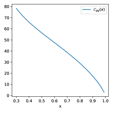
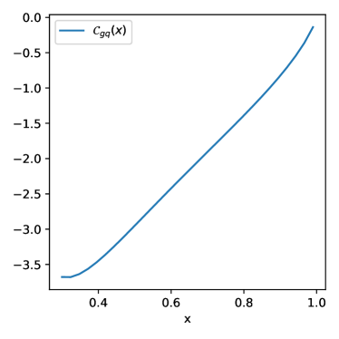
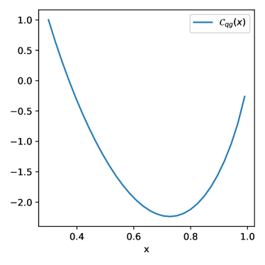
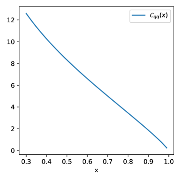
Figure 1: The NLO cumulants ${\cal C}_{ij}(x)$ Eq. (43). The gluon-gluon, gluon-quark, quark-gluon and quark-quark entries are shown from left to right and from top to bottom.

At NLO we only need two independent physical processes in order to fix the factorization scheme [10], and we then have a two-by-two quark-gluon matrix of coefficient functions $C^{(1),{\overline{\rm{MS}}}}_{ij}$ and thus of finite terms $C^{(1),{\overline{\rm{MS}}}}_{F,ij}$ and cumulants ${\cal C}_{ij}$. Using in particular the same processes as in Ref. [10] in order to define the physical scheme, namely deep-inelastic scattering and Higgs production in gluon fusion we get the matrix of cumulants that is shown in Fig. 1. It is clear that in practice the gluon-gluon entry dominates the perturbativity condition. Imposing the condition at $x=0.9$, so requiring $\frac{\alpha_{s}}{2\pi}{\cal C}_{gg}(x)<1$, we get $\alpha_{s}(Q^{2})\lesssim\frac{1}{3}$, corresponding to $Q^{2}\gtrsim 2$ GeV², which is a standard perturbativity condition. For comparison, in the NNPDF4.0 PDF determination positivity conditions are imposed at $Q^{2}=5$ GeV².

5 Conclusion

In this paper we have reviewed, expanded and made more quantitative our previous argument for the positivity of PDFs in the $\overline{\rm{MS}}$ scheme. Our main conclusion is that PDF positivity in the $\overline{\rm{MS}}$ scheme can be proven by defining PDFs in terms of physical processes, as it is done when choosing a physical factorization scheme, such as the DIS scheme [7, 8, 9, 10, 11]. We have then proven that $\overline{\rm{MS}}$ PDFs are always positive provided only the leading twist approximation is valid, and one is in a perturbative domain in which NLO corrections to the processes that are used to define the PDFs are smaller than the LO. We have conservatively estimated the scale where this is the case to be around $Q^{2}\gtrsim 2$ GeV², in keeping with standard QCD lore.

We have also made contact with recent arguments on PDF positivity of Ref. [2], through an explicit model computation, whose results agree with those of that reference. Namely, positivity of the collinear-unsubtracted PDF, and consequently positivity of the leading-twist, perturbatively computed structure functions and parton distributions only hold at high-enough scale. For an off-shell quark target this scale is about twice the target virtuality. For a hadronic target it cannot be computed perturbatively, though the model computation suggests that it is of order of the characteristic scale of the target. On the other hand, the definition of PDFs in terms of a physical scheme relies only on perturbation theory, and leads to the aforementioned conclusion that $\overline{\rm{MS}}$ PDFs are positive for scales above a few GeV. Clearly, all these arguments can only be established within the context of perturbative QCD factorization.

All results presented in this paper apply to massless quarks. It would be interesting to extend the discussion to the case of heavy quarks. This would be particularly interesting in view of recent results providing evidence for an intrinsic charm component of the proton [15], and also in view of subtle issues related to the validity of factorization for hadronic processes with heavy quarks in the initial state [16]. This will be left to future investigations.

Acknowledgements: A.C., S.F. and F.H. are supported by the European Research Council under the European Union’s Horizon 2020 research and innovation Programme (grant agreement n.740006); T.G. is supported by NWO via an ENW-KLEIN-2 project. We thank Luigi Del Debbio, Ted Rogers and Nobuo Sato for discussions.

Appendix A Perturbative computation of the bare PDF

The explicit expression of the fully bare quark PDF of an off-shell massless quark can be obtained by defining the PDF as the matrix element of a Wilson line operator [17], see Eq. (2.2) of Ref. [1], and evaluating this matrix element in a free off-shell massless quark state. The matrix element can be computed perturbatively using the Feynman rules for Wilson lines (see Sect. 7.6 of Ref. [4]). The computation is then similar to that presented in Sect. 9.4.3 of this reference, in the case of a massless, off-shell quark. Working in dimensional regularization we get, for a target quark with virtuality $M^{2}$,

$$f^{M,\,0}_{q/q} \left(x,\mu^{2},\epsilon\right)=\delta(1-x)\,Z$$

$$+2\pi\,g^{2}\mu^{2\epsilon}C_{F}\left(1-x\right)\int\frac{d^{2-2\epsilon}\bf{k}_{\text{T}}}{\left(2\pi\right)^{4-2\epsilon}}\,\frac{\left(1-\epsilon\right)\left(k_{\text{T}}^{2}+x^{2}M^{2}\right)}{\left(k_{\text{T}}^{2}-x\left(1-x\right)M^{2}\right)^{2}}$$

$$+4\pi\,g^{2}\mu^{2\epsilon}C_{F}\biggl{[}\frac{x}{\left(1-x\right)}\int\frac{d^{2-2\epsilon}\bf{k}_{\text{T}}}{\left(2\pi\right)^{4-2\epsilon}}\frac{1}{k_{\text{T}}^{2}-x\left(1-x\right)M^{2}}$$

$$\qquad\qquad-\,\delta\left(1-x\right)\int_{0}^{1}d\alpha\frac{\alpha}{\left(1-\alpha\right)}\int\frac{d^{2-2\epsilon}\bf{k}_{\text{T}}}{\left(2\pi\right)^{4-2\epsilon}}\frac{1}{k_{\text{T}}^{2}-\alpha\left(1-\alpha\right)M^{2}}\biggr{]}$$ (44)

where $Z$ is the residue in the pole of the quark propagator, given by

$$Z=1-g^{2}\mu^{2\epsilon}C_{F}\left(2-2\epsilon\right)\int_{0}^{1}dx\,\left(1-x\right)\int\frac{d^{4-2\epsilon}{\bf k}}{\left(2\pi\right)^{4-2\epsilon}}\frac{1}{\left(-k^{2}-x\left(1-x\right)M^{2}\right)^{2}}.$$ (45)

A direct computation of the different terms gives

$$f^{M,\,0}_{q/q}\left(x,\mu^{2},\epsilon\right)= \delta\left(1-x\right)+\frac{\alpha_{s}}{2\pi}C_{F}\left\{\Gamma\left(\epsilon\right)\,\left[\left(\frac{\Delta^{2}\left(x\right)}{4\pi\mu^{2}}\right)^{-\epsilon}p_{qq}\left(x\right)\right]_{+}+f_{f}(x)\right\},$$ (46)

where $p_{qq}\left(x\right)$ is as in Eq. (5), $\Delta^{2}\left(x\right)$ is given by Eq. (6), $\alpha_{s}=\frac{g^{2}}{4\pi}$, and $f_{f}(x)$ is a finite contribution given by

$$f_{f}(x)=\frac{1}{2}\delta\left(1-x\right)+x-2.$$ (47)

References

- [1] A. Candido, S. Forte, and F. Hekhorn, Can parton distributions be negative?, JHEP 11 (2020) 129, [arXiv:2006.07377].
- [2] J. Collins, T. C. Rogers, and N. Sato, Positivity and renormalization of parton densities, Phys. Rev. D 105 (2022), no. 7 076010, [arXiv:2111.01170].
- [3] J. C. Collins, D. E. Soper, and G. F. Sterman, Factorization of Hard Processes in QCD, Adv. Ser. Direct. High Energy Phys. 5 (1989) 1–91, [hep-ph/0409313].
- [4] J. Collins, Foundations of perturbative QCD, vol. 32. Cambridge University Press, 11, 2013.
- [5] F. Aslan, L. Gamberg, J. O. Gonzalez-Hernandez, T. Rainaldi, and T. C. Rogers, Basics of factorization in a scalar Yukawa field theory, Phys. Rev. D 107 (2023), no. 7 074031, [arXiv:2212.00757].
- [6] J. C. Collins, Renormalization: An Introduction to Renormalization, The Renormalization Group, and the Operator Product Expansion, vol. 26 of Cambridge Monographs on Mathematical Physics. Cambridge University Press, Cambridge, 1986.
- [7] M. Diemoz, F. Ferroni, E. Longo, and G. Martinelli, Parton Densities from Deep Inelastic Scattering to Hadronic Processes at Super Collider Energies, Z. Phys. C 39 (1988) 21.
- [8] S. Catani, Comment on quarks and gluons at small x and the SDIS factorization scheme, Z. Phys. C 70 (1996) 263–272, [hep-ph/9506357].
- [9] S. Catani, Physical anomalous dimensions at small x, Z. Phys. C 75 (1997) 665–678, [hep-ph/9609263].
- [10] G. Altarelli, S. Forte, and G. Ridolfi, On positivity of parton distributions, Nucl. Phys. B534 (1998) 277–296, [hep-ph/9806345].
- [11] T. Lappi, H. Mäntysaari, H. Paukkunen, and M. Tevio, Evolution of structure functions in momentum space, arXiv:2304.06998.
- [12] G. F. Sterman, Summation of Large Corrections to Short Distance Hadronic Cross-Sections, Nucl. Phys. B281 (1987) 310–364.
- [13] S. Catani and L. Trentadue, Resummation of the QCD Perturbative Series for Hard Processes, Nucl. Phys. B327 (1989) 323–352.
- [14] G. Altarelli, R. D. Ball, and S. Forte, Small x Resummation with Quarks: Deep-Inelastic Scattering, Nucl. Phys. B 799 (2008) 199–240, [arXiv:0802.0032].
- [15] NNPDF Collaboration, R. D. Ball, A. Candido, J. Cruz-Martinez, S. Forte, T. Giani, F. Hekhorn, K. Kudashkin, G. Magni, and J. Rojo, Evidence for intrinsic charm quarks in the proton, Nature 608 (2022), no. 7923 483–487, [arXiv:2208.08372].
- [16] F. Caola, K. Melnikov, D. Napoletano, and L. Tancredi, Noncancellation of infrared singularities in collisions of massive quarks, Phys. Rev. D 103 (2021), no. 5 054013, [arXiv:2011.04701].
- [17] J. C. Collins and D. E. Soper, Parton Distribution and Decay Functions, Nucl. Phys. B194 (1982) 445–492.