Back-to-back inclusive dijets in DIS at small x 𝑥 x
Paul Caucal
caucal@subatech.in2p3.fr
SUBATECH UMR 6457 (IMT Atlantique, Université de Nantes, IN2P3/CNRS), 4 rue Alfred Kastler,44307 Nantes, France
Farid Salazar
salazar@lbl.gov
Nuclear Science Division, Lawrence Berkeley National Laboratory, Berkeley, California 94720, USA
Physics Department, University of California, Berkeley, California 94720, USA
Department of Physics and Astronomy, University of California, Los Angeles, California 90095, USA
Mani L. Bhaumik Institute for Theoretical Physics, University of California, Los Angeles, California 90095, USA
Björn Schenke
bschenke@bnl.gov
Physics Department, Brookhaven National Laboratory, Upton, NY 11973, USA
Tomasz Stebel
tomasz.stebel@uj.edu.pl
Institute of Theoretical Physics, Jagiellonian University, ul. Lojasiewicza 11, 30-348 Kraków Poland
Raju Venugopalan
raju@bnl.gov
Physics Department, Brookhaven National Laboratory, Upton, NY 11973, USA
Abstract
We compute the back-to-back dijet cross-section in deep inelastic scattering (DIS) at small x 𝑥 x P ⟂ subscript 𝑃 perpendicular-to P_{\perp} q ⟂ subscript 𝑞 perpendicular-to q_{\perp} x 𝑥 x
The transverse momentum dependent gluon Weizsäcker-Williams distribution (WW TMD) is an object of fundamental interest in QCD [1 ] . A particularly interesting feature is the prediction [2 , 3 , 4 ] that in contrast to the WW photon distribution in QED, strong nonlinear gluon self-interactions in QCD at small x 𝑥 x k ⟂ ≲ Q s less-than-or-similar-to subscript 𝑘 perpendicular-to subscript 𝑄 𝑠 k_{\perp}\lesssim Q_{s} Q s ( x ) subscript 𝑄 𝑠 𝑥 Q_{s}(x) [5 , 6 ] .
A golden channel to extract the WW TMD is the inclusive
measurement of back-to-back jets (or hadrons) in deeply inelastic electron-nucleus scattering (e+A DIS), [7 , 8 ] characterized by the relative transverse momentum P ⟂ subscript 𝑃 perpendicular-to P_{\perp} q ⟂ subscript 𝑞 perpendicular-to q_{\perp} P ⟂ ≫ q ⟂ ≫ Λ QCD much-greater-than subscript 𝑃 perpendicular-to subscript 𝑞 perpendicular-to much-greater-than subscript Λ QCD P_{\perp}\gg q_{\perp}\gg\Lambda_{\rm QCD} Λ QCD subscript Λ QCD \Lambda_{\rm QCD} [8 ] . At next-to-leading-order (NLO) in the QCD coupling α s subscript 𝛼 𝑠 \alpha_{s} α s ln 2 ( P ⟂ / q ⟂ ) subscript 𝛼 𝑠 superscript 2 subscript 𝑃 perpendicular-to subscript 𝑞 perpendicular-to \alpha_{s}\ln^{2}(P_{\perp}/q_{\perp}) P ⟂ ≫ q ⟂ much-greater-than subscript 𝑃 perpendicular-to subscript 𝑞 perpendicular-to P_{\perp}\gg q_{\perp} [9 , 10 , 11 , 12 , 13 , 14 , 15 , 16 , 17 ] . NLO effects in gluon radiation also generate large small x 𝑥 x [15 , 16 , 17 ] . It is therefore critical to understand the interplay of these effects in the extraction of the WW gluon TMD.
In this letter, we will demonstrate within the framework of the Color Glass Condensate effective field theory (CGC EFT) [18 , 19 , 20 ] that TMD factorization of the inclusive back-to-back dijet cross-section in DIS at small x 𝑥 x q ⟂ / P ⟂ subscript 𝑞 perpendicular-to subscript 𝑃 perpendicular-to q_{\perp}/P_{\perp} Q s / P ⟂ subscript 𝑄 𝑠 subscript 𝑃 perpendicular-to Q_{s}/P_{\perp} Q s / q ⟂ subscript 𝑄 𝑠 subscript 𝑞 perpendicular-to Q_{s}/q_{\perp} x 𝑥 x P ⟂ / q ⟂ subscript 𝑃 perpendicular-to subscript 𝑞 perpendicular-to P_{\perp}/q_{\perp} P ⟂ subscript 𝑃 perpendicular-to P_{\perp} Q 2 superscript 𝑄 2 Q^{2}
We will apply our results
to the kinematics of the future Electron-Ion Collider (EIC) [22 , 23 , 24 ] . While dijet studies are challenging at small x 𝑥 x [25 , 26 , 27 , 28 , 29 , 30 ] , a window in the required phase space may exist for this theoretically robust final state. The extension of our study to the phenomenologically more accessible [31 ] , if theoretically less robust, di-hadron final state is straightforward [32 ] . Our computation is the first to include all above listed NLO components to determine the relative impact of Sudakov suppression and gluon saturation.
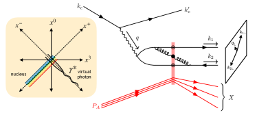
In the dipole frame with virtual photon four-momentum q μ = ( − Q 2 / ( 2 q − ) , q − , 𝟎 ⟂ ) superscript 𝑞 𝜇 superscript 𝑄 2 2 superscript 𝑞 superscript 𝑞 subscript 0 perpendicular-to q^{\mu}=(-Q^{2}/(2q^{-}),q^{-},\boldsymbol{0}_{\perp}) P μ = ( P + , 0 , 𝟎 ⟂ ) superscript 𝑃 𝜇 superscript 𝑃 0 subscript 0 perpendicular-to P^{\mu}=(P^{+},0,\boldsymbol{0}_{\perp}) d σ LO λ = z 1 z 2 d σ LO λ d 2 𝑷 ⟂ d 2 𝒒 ⟂ d z 1 d z 2 d subscript superscript 𝜎 𝜆 LO subscript 𝑧 1 subscript 𝑧 2 d subscript superscript 𝜎 𝜆 LO superscript d 2 subscript 𝑷 perpendicular-to superscript d 2 subscript 𝒒 perpendicular-to d subscript 𝑧 1 d subscript 𝑧 2 \mathrm{d}\sigma^{\lambda}_{\rm LO}=z_{1}z_{2}\frac{\mathrm{d}\sigma^{\lambda}_{\rm LO}}{\mathrm{d}^{2}\boldsymbol{P}_{\perp}\mathrm{d}^{2}\boldsymbol{q}_{\perp}\mathrm{d}z_{1}\mathrm{d}z_{2}} [8 , 33 ]
⟨ d σ LO λ ⟩ = ∫ d 2 𝒓 ⟂ d 2 𝒓 ⟂ ′ d 2 𝒃 ⟂ d 2 𝒃 ⟂ ′ e − i 𝑷 ⟂ ⋅ ( 𝒓 ⟂ − 𝒓 ⟂ ′ ) delimited-⟨⟩ d subscript superscript 𝜎 𝜆 LO superscript d 2 subscript 𝒓 perpendicular-to superscript d 2 superscript subscript 𝒓 perpendicular-to ′ superscript d 2 subscript 𝒃 perpendicular-to superscript d 2 superscript subscript 𝒃 perpendicular-to ′ superscript 𝑒 ⋅ 𝑖 subscript 𝑷 perpendicular-to subscript 𝒓 perpendicular-to superscript subscript 𝒓 perpendicular-to ′ \displaystyle\langle\mathrm{d}\sigma^{\lambda}_{\mathrm{LO}}\rangle=\int\mathrm{d}^{2}\boldsymbol{r}_{\perp}\mathrm{d}^{2}\boldsymbol{r}_{\perp}^{\prime}\mathrm{d}^{2}\boldsymbol{b}_{\perp}\mathrm{d}^{2}\boldsymbol{b}_{\perp}^{\prime}e^{-i\boldsymbol{P}_{\perp}\cdot(\boldsymbol{r}_{\perp}-\boldsymbol{r}_{\perp}^{\prime})}
× e − i 𝒒 ⟂ ⋅ ( 𝒃 ⟂ − 𝒃 ⟂ ′ ) ℛ λ ( 𝒓 ⟂ , 𝒓 ⟂ ′ ) ⟨ Ξ ( 𝒓 ⟂ , 𝒓 ⟂ ′ , 𝒃 ⟂ , 𝒃 ⟂ ′ ) ⟩ , absent superscript 𝑒 ⋅ 𝑖 subscript 𝒒 perpendicular-to subscript 𝒃 perpendicular-to superscript subscript 𝒃 perpendicular-to ′ superscript ℛ 𝜆 subscript 𝒓 perpendicular-to superscript subscript 𝒓 perpendicular-to ′ delimited-⟨⟩ Ξ subscript 𝒓 perpendicular-to superscript subscript 𝒓 perpendicular-to ′ subscript 𝒃 perpendicular-to superscript subscript 𝒃 perpendicular-to ′ \displaystyle\times e^{-i\boldsymbol{q}_{\perp}\cdot(\boldsymbol{b}_{\perp}-\boldsymbol{b}_{\perp}^{\prime})}\mathcal{R}^{\lambda}(\boldsymbol{r}_{\perp},\boldsymbol{r}_{\perp}^{\prime})\langle\Xi(\boldsymbol{r}_{\perp},\boldsymbol{r}_{\perp}^{\prime},\boldsymbol{b}_{\perp},\boldsymbol{b}_{\perp}^{\prime})\rangle\,, (1)
where λ = L , T 𝜆 L T
\lambda=\rm L,T 𝑷 ⟂ = z 2 𝒌 𝟏 ⟂ − z 1 𝒌 𝟐 ⟂ subscript 𝑷 perpendicular-to subscript 𝑧 2 subscript 𝒌 perpendicular-to 1 absent subscript 𝑧 1 subscript 𝒌 perpendicular-to 2 absent \boldsymbol{P}_{\perp}=z_{2}\boldsymbol{k_{1\perp}}-z_{1}\boldsymbol{k_{2\perp}} 𝒒 ⟂ = 𝒌 𝟏 ⟂ + 𝒌 𝟐 ⟂ subscript 𝒒 perpendicular-to subscript 𝒌 perpendicular-to 1 absent subscript 𝒌 perpendicular-to 2 absent \boldsymbol{q}_{\perp}=\boldsymbol{k_{1\perp}}+\boldsymbol{k_{2\perp}} z i = k i − / q − subscript 𝑧 𝑖 superscript subscript 𝑘 𝑖 superscript 𝑞 z_{i}=k_{i}^{-}/q^{-} ℛ λ superscript ℛ 𝜆 \mathcal{R}^{\lambda} Ξ Ξ \Xi ⟨ … ⟩ delimited-⟨⟩ … \langle\dots\rangle x 𝑥 x
Figure 1: NLO DIS diagram for dijet production in dipole scattering off shockwave (red rectangle) in the CGC EFT. The nuclear target and the virtual photon move close to the lightcone with large q − superscript 𝑞 q^{-} P A + superscript subscript 𝑃 𝐴 P_{A}^{+}
The one-loop (1L) correction to Eq. (1 1 [33 ]
α s d σ 1 L λ = α s ∫ z 0 1 d z g z g ∫ d 2 𝒛 ⟂ d σ ~ 1 L λ ( z g , 𝒛 ⟂ ) , subscript 𝛼 𝑠 d subscript superscript 𝜎 𝜆 1 L subscript 𝛼 𝑠 superscript subscript subscript 𝑧 0 1 d subscript 𝑧 𝑔 subscript 𝑧 𝑔 superscript d 2 subscript 𝒛 perpendicular-to differential-d subscript superscript ~ 𝜎 𝜆 1 L subscript 𝑧 𝑔 subscript 𝒛 perpendicular-to \displaystyle\alpha_{s}\mathrm{d}\sigma^{\lambda}_{1\mathrm{L}}=\alpha_{s}\int_{z_{0}}^{1}\frac{\mathrm{d}z_{g}}{z_{g}}\int\mathrm{d}^{2}\boldsymbol{z}_{\perp}\mathrm{d}\widetilde{\sigma}^{\lambda}_{1\mathrm{L}}(z_{g},\boldsymbol{z}_{\perp})\,, (2)
where z g = k g − / q − subscript 𝑧 𝑔 superscript subscript 𝑘 𝑔 superscript 𝑞 z_{g}=k_{g}^{-}/q^{-} k g − superscript subscript 𝑘 𝑔 k_{g}^{-} 𝒛 ⟂ subscript 𝒛 perpendicular-to \boldsymbol{z}_{\perp} z 0 ∝ 1 / s proportional-to subscript 𝑧 0 1 𝑠 z_{0}\propto 1/s z g subscript 𝑧 𝑔 z_{g} [33 ] . The integrand satisfies α s ∫ 𝒛 ⟂ d σ ~ 1 L ( 0 , 𝒛 ⟂ ) = H LL d σ LO subscript 𝛼 𝑠 subscript subscript 𝒛 perpendicular-to differential-d subscript ~ 𝜎 1 L 0 subscript 𝒛 perpendicular-to subscript 𝐻 LL d subscript 𝜎 LO \alpha_{s}\int_{\boldsymbol{z}_{\perp}}\mathrm{d}\widetilde{\sigma}_{1\mathrm{L}}(0,\boldsymbol{z}_{\perp})=H_{\mathrm{LL}}\mathrm{d}\sigma_{\mathrm{LO}} x 𝑥 x [34 , 35 , 36 , 37 , 38 , 39 , 40 ]
H LL = α s N c 2 π 2 ∫ 𝒛 ⟂ 𝒦 LL , subscript 𝐻 LL subscript 𝛼 𝑠 subscript 𝑁 𝑐 2 superscript 𝜋 2 subscript subscript 𝒛 perpendicular-to subscript 𝒦 LL \displaystyle H_{\mathrm{LL}}=\frac{\alpha_{s}N_{c}}{2\pi^{2}}\int_{\boldsymbol{z}_{\perp}}\mathcal{K}_{\mathrm{LL}}\,, (3)
where 𝒦 LL subscript 𝒦 LL \mathcal{K}_{\mathrm{LL}} x 𝑥 x 2
α s d σ 1 L λ subscript 𝛼 𝑠 d subscript superscript 𝜎 𝜆 1 L \displaystyle\alpha_{s}\mathrm{d}\sigma^{\lambda}_{1\mathrm{L}} = ln ( z f z 0 ) H LL d σ LO λ + α s ∫ 0 1 d z g z g ∫ d 2 𝒛 ⟂ absent subscript 𝑧 𝑓 subscript 𝑧 0 subscript 𝐻 LL d subscript superscript 𝜎 𝜆 LO subscript 𝛼 𝑠 superscript subscript 0 1 d subscript 𝑧 𝑔 subscript 𝑧 𝑔 superscript d 2 subscript 𝒛 perpendicular-to \displaystyle=\ln\left(\frac{z_{f}}{z_{0}}\right)H_{\mathrm{LL}}\mathrm{d}\sigma^{\lambda}_{\mathrm{LO}}+\alpha_{s}\int_{0}^{1}\frac{\mathrm{d}z_{g}}{z_{g}}\int\mathrm{d}^{2}\boldsymbol{z}_{\perp}
[ d σ ~ 1 L λ ( z g , 𝒛 ⟂ ) − d σ ~ 1 L λ ( 0 , 𝒛 ⟂ ) Θ ( z f − z g ) ] . delimited-[] d subscript superscript ~ 𝜎 𝜆 1 L subscript 𝑧 𝑔 subscript 𝒛 perpendicular-to d subscript superscript ~ 𝜎 𝜆 1 L 0 subscript 𝒛 perpendicular-to Θ subscript 𝑧 𝑓 subscript 𝑧 𝑔 \displaystyle\Big{[}\mathrm{d}\widetilde{\sigma}^{\lambda}_{1\mathrm{L}}(z_{g},\boldsymbol{z}_{\perp})-\mathrm{d}\widetilde{\sigma}^{\lambda}_{1\mathrm{L}}(0,\boldsymbol{z}_{\perp})\Theta(z_{f}-z_{g})\Big{]}\,. (4)
The first term isolates the large projectile-rapidity logarithm by introducing an arbitrary z f ≡ k f − / q − subscript 𝑧 𝑓 superscript subscript 𝑘 𝑓 superscript 𝑞 z_{f}\equiv k_{f}^{-}/q^{-} z g ≥ z f subscript 𝑧 𝑔 subscript 𝑧 𝑓 z_{g}\geq z_{f} z g ≤ z f subscript 𝑧 𝑔 subscript 𝑧 𝑓 z_{g}\leq z_{f} z f subscript 𝑧 𝑓 z_{f} x 𝑥 x α s ln ( z f / z 0 ) subscript 𝛼 𝑠 subscript 𝑧 𝑓 subscript 𝑧 0 \alpha_{s}\ln(z_{f}/z_{0}) Y f = ln ( z f ) subscript 𝑌 𝑓 subscript 𝑧 𝑓 Y_{f}=\ln(z_{f})
∂ ⟨ d σ LO ⟩ Y f ∂ Y f = ⟨ H LL d σ LO ⟩ Y f . subscript delimited-⟨⟩ d subscript 𝜎 LO subscript 𝑌 𝑓 subscript 𝑌 𝑓 subscript delimited-⟨⟩ subscript 𝐻 LL d subscript 𝜎 LO subscript 𝑌 𝑓 \displaystyle\frac{\partial\langle\mathrm{d}\sigma_{\rm LO}\rangle_{Y_{f}}}{\partial Y_{f}}=\left\langle H_{\mathrm{LL}}\mathrm{d}\sigma_{\rm LO}\right\rangle_{Y_{f}}\,. (5)
The second term in Eq. (4 ⟨ d σ NLO ⟩ Y f subscript delimited-⟨⟩ d subscript 𝜎 NLO subscript 𝑌 𝑓 \langle\mathrm{d}\sigma_{\rm NLO}\rangle_{Y_{f}} z 0 ∝ 1 / s → 0 proportional-to subscript 𝑧 0 1 𝑠 → 0 z_{0}\propto 1/s\to 0 s 𝑠 \sqrt{s} Y f subscript 𝑌 𝑓 Y_{f} x 𝑥 x x 𝑥 x H LL → H LL + α s H NLL → subscript 𝐻 LL subscript 𝐻 LL subscript 𝛼 𝑠 subscript 𝐻 NLL H_{\mathrm{LL}}\to H_{\mathrm{LL}}+\alpha_{s}H_{\textrm{NLL}} [42 , 43 , 44 , 45 ] on the LO cross-section since the α s 2 ln ( z f / z 0 ) superscript subscript 𝛼 𝑠 2 subscript 𝑧 𝑓 subscript 𝑧 0 \alpha_{s}^{2}\ln(z_{f}/z_{0}) ⟨ d σ NLO ⟩ Y f subscript delimited-⟨⟩ d subscript 𝜎 NLO subscript 𝑌 𝑓 \langle\mathrm{d}\sigma_{\rm NLO}\rangle_{Y_{f}}
We turn now to the back-to-back limit of the NLO inclusive dijet result in [33 ] .
At LO, it was shown to have the TMD factorized form [8 ]
⟨ d σ LO λ , b2b ⟩ Y 0 = ℋ LO λ , i j ∫ 𝒃 ⟂ , 𝒃 ⟂ ′ e − i 𝒒 ⟂ ⋅ 𝒓 b b ′ ( 2 π ) 4 G ^ Y 0 i j ( 𝒓 b b ′ , μ ) , subscript delimited-⟨⟩ d subscript superscript 𝜎 𝜆 b2b
LO subscript 𝑌 0 superscript subscript ℋ LO 𝜆 𝑖 𝑗
subscript subscript 𝒃 perpendicular-to superscript subscript 𝒃 perpendicular-to ′
superscript 𝑒 ⋅ 𝑖 subscript 𝒒 perpendicular-to subscript 𝒓 𝑏 superscript 𝑏 ′ superscript 2 𝜋 4 subscript superscript ^ 𝐺 𝑖 𝑗 subscript 𝑌 0 subscript 𝒓 𝑏 superscript 𝑏 ′ 𝜇 \displaystyle\langle\mathrm{d}\sigma^{\lambda,\mathrm{b2b}}_{\rm LO}\rangle_{Y_{0}}=\mathcal{H}_{\rm LO}^{\lambda,ij}\int_{\boldsymbol{b}_{\perp},\boldsymbol{b}_{\perp}^{\prime}}\frac{e^{-i\boldsymbol{q}_{\perp}\cdot\boldsymbol{r}_{bb^{\prime}}}}{(2\pi)^{4}}\hat{G}^{ij}_{Y_{0}}(\boldsymbol{r}_{bb^{\prime}},\mu)\,, (6)
with 𝒓 b b ′ = 𝒃 ⟂ − 𝒃 ⟂ ′ subscript 𝒓 𝑏 superscript 𝑏 ′ subscript 𝒃 perpendicular-to superscript subscript 𝒃 perpendicular-to ′ \boldsymbol{r}_{bb^{\prime}}=\boldsymbol{b}_{\perp}-\boldsymbol{b}_{\perp}^{\prime} ℋ LO λ , i j superscript subscript ℋ LO 𝜆 𝑖 𝑗
\mathcal{H}_{\rm LO}^{\lambda,ij} 𝑷 ⟂ subscript 𝑷 perpendicular-to \boldsymbol{P}_{\perp} Q 𝑄 Q z i subscript 𝑧 𝑖 z_{i} Y 0 = ln ( z 0 ) subscript 𝑌 0 subscript 𝑧 0 Y_{0}=\ln(z_{0})
G ^ Y 0 i j ( 𝒓 b b ′ , μ ) ≡ − 2 α s ( μ ) ⟨ Tr [ V 𝒃 ⟂ ∂ i V 𝒃 ⟂ † V 𝒃 ⟂ ′ ∂ j V 𝒃 ⟂ ′ † ] ⟩ Y 0 , subscript superscript ^ 𝐺 𝑖 𝑗 subscript 𝑌 0 subscript 𝒓 𝑏 superscript 𝑏 ′ 𝜇 2 subscript 𝛼 𝑠 𝜇 subscript delimited-⟨⟩ Tr delimited-[] subscript 𝑉 subscript 𝒃 perpendicular-to superscript 𝑖 subscript superscript 𝑉 † subscript 𝒃 perpendicular-to subscript 𝑉 superscript subscript 𝒃 perpendicular-to ′ superscript 𝑗 subscript superscript 𝑉 † superscript subscript 𝒃 perpendicular-to ′ subscript 𝑌 0 \displaystyle\hat{G}^{ij}_{Y_{0}}(\boldsymbol{r}_{bb^{\prime}},\mu)\equiv\frac{-2}{\alpha_{s}(\mu)}\left\langle\mathrm{Tr}\left[V_{\boldsymbol{b}_{\perp}}\partial^{i}V^{\dagger}_{\boldsymbol{b}_{\perp}}V_{\boldsymbol{b}_{\perp}^{\prime}}\partial^{j}V^{\dagger}_{\boldsymbol{b}_{\perp}^{\prime}}\right]\right\rangle_{Y_{0}}\!\!\,, (7)
with V 𝒃 ⟂ subscript 𝑉 subscript 𝒃 perpendicular-to V_{\boldsymbol{b}_{\perp}} 𝒃 ⟂ subscript 𝒃 perpendicular-to \boldsymbol{b}_{\perp} μ 𝜇 \mu μ ∼ Q s similar-to 𝜇 subscript 𝑄 𝑠 \mu\sim Q_{s} q ⟂ ∼ Q s similar-to subscript 𝑞 perpendicular-to subscript 𝑄 𝑠 q_{\perp}\sim Q_{s}
As in the LO case [46 , 47 , 28 , 29 , 48 ] , we can extract the NLO impact factor for inclusive back-to-back dijets from the LP contributions (q ⟂ , Q s ≪ P ⟂ much-less-than subscript 𝑞 perpendicular-to subscript 𝑄 𝑠
subscript 𝑃 perpendicular-to q_{\perp},Q_{s}\ll P_{\perp} ⟨ d σ NLO λ ⟩ Y f subscript delimited-⟨⟩ d subscript superscript 𝜎 𝜆 NLO subscript 𝑌 𝑓 \langle\mathrm{d}\sigma^{\lambda}_{\rm NLO}\rangle_{Y_{f}} [33 ] . Remarkably, these are
also proportional to the WW gluon TMD [49 ] , with dominant contributions to the impact factor from the Sudakov logarithms α s ln 2 ( P ⟂ r b b ′ ) subscript 𝛼 𝑠 superscript 2 subscript 𝑃 perpendicular-to subscript 𝑟 𝑏 superscript 𝑏 ′ \alpha_{s}\ln^{2}(P_{\perp}r_{bb^{\prime}}) α s ln ( P ⟂ r b b ′ ) subscript 𝛼 𝑠 subscript 𝑃 perpendicular-to subscript 𝑟 𝑏 superscript 𝑏 ′ \alpha_{s}\ln(P_{\perp}r_{bb^{\prime}}) P ⟂ / q ⟂ ≫ 1 much-greater-than subscript 𝑃 perpendicular-to subscript 𝑞 perpendicular-to 1 P_{\perp}/q_{\perp}\gg 1 𝒪 ( α s ) 𝒪 subscript 𝛼 𝑠 \mathcal{O}(\alpha_{s}) 2 4 ln 2 ( z 0 ) superscript 2 subscript 𝑧 0 \ln^{2}(z_{0}) z g → 0 → subscript 𝑧 𝑔 0 z_{g}\to 0 [50 , 51 ] :
α s d σ NLO λ , b2b = α s ∫ 0 1 d z g z g ∫ d 2 𝒛 ⟂ [ d σ ~ 1 L λ , b2b ( z g , 𝒛 ⟂ ) \displaystyle\alpha_{s}\mathrm{d}\sigma^{\lambda,\mathrm{b2b}}_{\mathrm{NLO}}=\alpha_{s}\int_{0}^{1}\frac{\mathrm{d}z_{g}}{z_{g}}\int\mathrm{d}^{2}\boldsymbol{z}_{\perp}\left[\mathrm{d}\widetilde{\sigma}^{\lambda,\mathrm{b2b}}_{1\mathrm{L}}(z_{g},\boldsymbol{z}_{\perp})\right.
− d σ ~ 1 L λ , b2b ( 0 , 𝒛 ⟂ ) Θ ( z f − z g ) Θ ( − ln ( z g ) − Δ c ) ] , \displaystyle\left.-\mathrm{d}\widetilde{\sigma}^{\lambda,\mathrm{b2b}}_{1\mathrm{L}}(0,\boldsymbol{z}_{\perp})\Theta(z_{f}-z_{g})\Theta\left(-\ln\left(z_{g}\right)-\Delta_{c}\right)\right]\,, (8)
where Δ c = ln ( min ( 𝒓 z b 2 , 𝒓 z b ′ 2 ) 2 k c + q − ) subscript Δ 𝑐 min superscript subscript 𝒓 𝑧 𝑏 2 superscript subscript 𝒓 𝑧 superscript 𝑏 ′ 2 2 superscript subscript 𝑘 𝑐 superscript 𝑞 \Delta_{c}=\ln(\textrm{min}(\boldsymbol{r}_{zb}^{2},\boldsymbol{r}_{zb^{\prime}}^{2})2k_{c}^{+}q^{-}) 𝒓 z b = 𝒛 ⟂ − 𝒃 ⟂ subscript 𝒓 𝑧 𝑏 subscript 𝒛 perpendicular-to subscript 𝒃 perpendicular-to \boldsymbol{r}_{zb}=\boldsymbol{z}_{\perp}-\boldsymbol{b}_{\perp} k c + = x c P + superscript subscript 𝑘 𝑐 subscript 𝑥 𝑐 superscript 𝑃 k_{c}^{+}=x_{c}P^{+} x c = 1 e c 0 2 M q q ¯ 2 + Q 2 W 2 + Q 2 subscript 𝑥 𝑐 1 𝑒 superscript subscript 𝑐 0 2 superscript subscript 𝑀 𝑞 ¯ 𝑞 2 superscript 𝑄 2 superscript 𝑊 2 superscript 𝑄 2 x_{c}=\frac{1}{ec_{0}^{2}}\frac{M_{q\bar{q}}^{2}+Q^{2}}{W^{2}+Q^{2}} Q 2 superscript 𝑄 2 Q^{2} W 𝑊 W M q q ¯ = P ⟂ / z 1 z 2 subscript 𝑀 𝑞 ¯ 𝑞 subscript 𝑃 perpendicular-to subscript 𝑧 1 subscript 𝑧 2 M_{q\bar{q}}=P_{\perp}/\sqrt{z_{1}z_{2}} c 0 = 2 e − γ E subscript 𝑐 0 2 superscript 𝑒 subscript 𝛾 𝐸 c_{0}=2e^{-\gamma_{E}} γ E subscript 𝛾 𝐸 \gamma_{E}
Comparing Eq. (8 4 x 𝑥 x 5 specifically for the WW gluon TMD is to modify the kernel
in the JIMWLK Hamiltonian [49 , 51 ] :
H LL k c d σ LO λ , b2b ≡ α s N c 2 π 2 ∫ 𝒛 ⟂ Θ ( − Y f − Δ c ) 𝒦 LL d σ LO λ , b2b . subscript superscript 𝐻 𝑘 𝑐 LL d subscript superscript 𝜎 𝜆 b2b
LO subscript 𝛼 𝑠 subscript 𝑁 𝑐 2 superscript 𝜋 2 subscript subscript 𝒛 perpendicular-to Θ subscript 𝑌 𝑓 subscript Δ 𝑐 subscript 𝒦 LL differential-d subscript superscript 𝜎 𝜆 b2b
LO \displaystyle H^{kc}_{\mathrm{LL}}\mathrm{d}\sigma^{\lambda,\rm b2b}_{\rm LO}\equiv\frac{\alpha_{s}N_{c}}{2\pi^{2}}\int_{\boldsymbol{z}_{\perp}}\Theta(-Y_{f}-\Delta_{c})\mathcal{K}_{\mathrm{LL}}\mathrm{d}\sigma^{\lambda,\rm b2b}_{\rm LO}\,. (9)
The Θ Θ \Theta 1 / k g + ∼ 2 k g − / 𝒌 ⟂ 2 ≤ 1 / k c + similar-to 1 superscript subscript 𝑘 𝑔 2 superscript subscript 𝑘 𝑔 superscript subscript 𝒌 perpendicular-to 2 1 superscript subscript 𝑘 𝑐 1/k_{g}^{+}\sim 2k_{g}^{-}/\boldsymbol{k}_{\perp}^{2}\leq 1/k_{c}^{+} 1 / k c + 1 superscript subscript 𝑘 𝑐 1/k_{c}^{+} 1 / | q + | 1 superscript 𝑞 1/|q^{+}| [52 , 53 ] and 𝒌 ⟂ 2 ∼ 1 / min ( 𝒓 z b ′ 2 , 𝒓 z b ′ 2 ) similar-to superscript subscript 𝒌 perpendicular-to 2 1 min superscript subscript 𝒓 𝑧 superscript 𝑏 ′ 2 superscript subscript 𝒓 𝑧 superscript 𝑏 ′ 2 \boldsymbol{k}_{\perp}^{2}\sim 1/\textrm{min}(\boldsymbol{r}_{zb^{\prime}}^{2},\boldsymbol{r}_{zb^{\prime}}^{2}) [54 , 55 , 56 , 57 , 58 , 59 , 60 , 61 , 62 , 63 , 64 ] to generate all-order resummation of transverse double logarithms
necessary to match small-x 𝑥 x 9 x 𝑥 x
On the surface, Eq. (9 k c + superscript subscript 𝑘 𝑐 k_{c}^{+} Y f subscript 𝑌 𝑓 Y_{f} η f = ln ( P + / k f + ) subscript 𝜂 𝑓 superscript 𝑃 superscript subscript 𝑘 𝑓 \eta_{f}=\ln(P^{+}/k_{f}^{+}) 9
η f = Y f + ln ( M q q ¯ 2 + Q 2 e P ⟂ 2 ) + ln ( 𝑷 ⟂ 2 𝒓 b b ′ 2 c 0 2 ) − ln ( x c ) , subscript 𝜂 𝑓 subscript 𝑌 𝑓 superscript subscript 𝑀 𝑞 ¯ 𝑞 2 superscript 𝑄 2 𝑒 superscript subscript 𝑃 perpendicular-to 2 superscript subscript 𝑷 perpendicular-to 2 superscript subscript 𝒓 𝑏 superscript 𝑏 ′ 2 superscript subscript 𝑐 0 2 subscript 𝑥 𝑐 \eta_{f}=Y_{f}+\ln\left(\frac{M_{q\bar{q}}^{2}+Q^{2}}{eP_{\perp}^{2}}\right)+\ln\left(\frac{\boldsymbol{P}_{\perp}^{2}\boldsymbol{r}_{bb^{\prime}}^{2}}{c_{0}^{2}}\right)-\ln(x_{c})\,, (10)
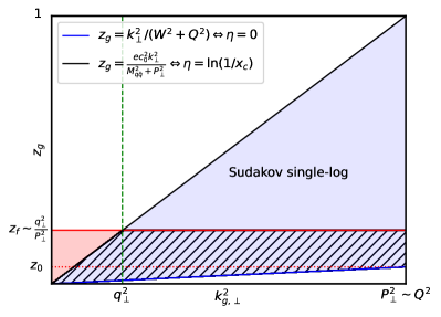
the Θ Θ \Theta 9 η f ≤ η c = ln ( 1 / x c ) subscript 𝜂 𝑓 subscript 𝜂 𝑐 1 subscript 𝑥 𝑐 \eta_{f}\leq\eta_{c}=\ln(1/x_{c}) η f subscript 𝜂 𝑓 \eta_{f} 9 η f subscript 𝜂 𝑓 \eta_{f} [65 , 66 , 67 ] described in the supplemental material.
Importantly, for scale choice η f ∼ ln ( 1 / x c ) similar-to subscript 𝜂 𝑓 1 subscript 𝑥 𝑐 \eta_{f}\sim\ln(1/x_{c}) Y f ∼ − ln ( 𝑷 ⟂ 2 𝒓 b b ′ 2 ) similar-to subscript 𝑌 𝑓 superscript subscript 𝑷 perpendicular-to 2 superscript subscript 𝒓 𝑏 superscript 𝑏 ′ 2 Y_{f}\sim-\ln(\boldsymbol{P}_{\perp}^{2}\boldsymbol{r}_{bb^{\prime}}^{2}) k f − ≤ k g − ≲ q − superscript subscript 𝑘 𝑓 superscript subscript 𝑘 𝑔 less-than-or-similar-to superscript 𝑞 k_{f}^{-}\leq k_{g}^{-}\lesssim q^{-} x 𝑥 x
The dijet cross-section is expanded in Fourier moments as d σ λ = d σ ( 0 ) , λ + 2 ∑ n = 1 ∞ d σ ( 2 n ) , λ cos ( 2 n ϕ ) d superscript 𝜎 𝜆 d superscript 𝜎 0 𝜆
2 superscript subscript 𝑛 1 d superscript 𝜎 2 𝑛 𝜆
2 𝑛 italic-ϕ \mathrm{d}\sigma^{\lambda}=\mathrm{d}\sigma^{(0),\lambda}+2\sum_{n=1}^{\infty}\mathrm{d}\sigma^{(2n),\lambda}\cos(2n\phi) ϕ italic-ϕ \phi 𝒒 ⟂ subscript 𝒒 perpendicular-to \boldsymbol{q}_{\perp} 𝑷 ⟂ subscript 𝑷 perpendicular-to \boldsymbol{P}_{\perp} [25 , 26 , 28 , 29 , 27 ] . To NLO accuracy, the azimuthally averaged back-to-back dijet cross-section has the TMD factorized expression
⟨ d σ LO ( 0 ) , λ , b2b + α s d σ NLO ( 0 ) , λ , b2b ⟩ η f subscript delimited-⟨⟩ d subscript superscript 𝜎 0 𝜆 b2b
LO subscript 𝛼 𝑠 d subscript superscript 𝜎 0 𝜆 b2b
NLO subscript 𝜂 𝑓 \displaystyle\left\langle\mathrm{d}\sigma^{(0),\lambda,\rm b2b}_{\rm LO}+\alpha_{s}\mathrm{d}\sigma^{(0),\lambda,\rm b2b}_{\rm NLO}\right\rangle_{\eta_{f}} = ℋ LO 0 , λ ∫ d 2 𝑩 ⟂ ( 2 π ) 2 ∫ d 2 𝒓 b b ′ ( 2 π ) 2 e − i 𝒒 ⟂ ⋅ 𝒓 b b ′ G ^ η f 0 ( 𝒓 b b ′ , μ 0 ) { 1 + α s ( μ R ) π [ − N c 4 ln 2 ( 𝑷 ⟂ 2 𝒓 b b ′ 2 c 0 2 ) ⏟ Sudakov double log \displaystyle=\mathcal{H}_{\rm LO}^{0,\lambda}\int\frac{\mathrm{d}^{2}\boldsymbol{B}_{\perp}}{(2\pi)^{2}}\int\frac{\mathrm{d}^{2}\boldsymbol{r}_{bb^{\prime}}}{(2\pi)^{2}}e^{-i\boldsymbol{q}_{\perp}\cdot\boldsymbol{r}_{bb^{\prime}}}\hat{G}^{0}_{\eta_{f}}(\boldsymbol{r}_{bb^{\prime}},\mu_{0})\Bigg{\{}1+\frac{\alpha_{s}(\mu_{R})}{\pi}\Big{[}\underbrace{-\frac{N_{c}}{4}\ln^{2}\left(\frac{\boldsymbol{P}_{\perp}^{2}\boldsymbol{r}_{bb^{\prime}}^{2}}{c_{0}^{2}}\right)}_{\mathrm{Sudakov\ double\ log}}
− s L ln ( 𝑷 ⟂ 2 𝒓 b b ′ 2 c 0 2 ) + β 0 ln ( μ R 2 𝒓 b b ′ 2 c 0 2 ) ⏟ Sudakov single logs + N c 2 f 1 λ ( χ , z 1 , R , η f ) + 1 2 N c f 2 λ ( χ , z 1 , R ) ] } \displaystyle\underbrace{-s_{L}\ln\left(\frac{\boldsymbol{P}_{\perp}^{2}\boldsymbol{r}_{bb^{\prime}}^{2}}{c_{0}^{2}}\right)+\beta_{0}\ln\left(\frac{\mu_{R}^{2}\boldsymbol{r}_{bb^{\prime}}^{2}}{c_{0}^{2}}\right)}_{\mathrm{Sudakov\ single\ logs}}+\frac{N_{c}}{2}f^{\lambda}_{1}(\chi,z_{1},R,\eta_{f})+\frac{1}{2N_{c}}f^{\lambda}_{2}(\chi,z_{1},R)\Big{]}\Bigg{\}}
+ α s ( μ R ) π ℋ LO 0 , λ ∫ d 2 𝑩 ⟂ ( 2 π ) 2 ∫ d 2 𝒓 b b ′ ( 2 π ) 2 e − i 𝒒 ⟂ ⋅ 𝒓 b b ′ h ^ η f 0 ( 𝒓 b b ′ , μ 0 ) { N c 2 [ 1 + ln ( R 2 ) ] − 1 2 N c ln ( z 1 z 2 R 2 ) } . subscript 𝛼 𝑠 subscript 𝜇 𝑅 𝜋 superscript subscript ℋ LO 0 𝜆
superscript d 2 subscript 𝑩 perpendicular-to superscript 2 𝜋 2 superscript d 2 subscript 𝒓 𝑏 superscript 𝑏 ′ superscript 2 𝜋 2 superscript 𝑒 ⋅ 𝑖 subscript 𝒒 perpendicular-to subscript 𝒓 𝑏 superscript 𝑏 ′ subscript superscript ^ ℎ 0 subscript 𝜂 𝑓 subscript 𝒓 𝑏 superscript 𝑏 ′ subscript 𝜇 0 subscript 𝑁 𝑐 2 delimited-[] 1 superscript 𝑅 2 1 2 subscript 𝑁 𝑐 subscript 𝑧 1 subscript 𝑧 2 superscript 𝑅 2 \displaystyle+\frac{\alpha_{s}(\mu_{R})}{\pi}\mathcal{H}_{\rm LO}^{0,\lambda}\int\frac{\mathrm{d}^{2}\boldsymbol{B}_{\perp}}{(2\pi)^{2}}\int\frac{\mathrm{d}^{2}\boldsymbol{r}_{bb^{\prime}}}{(2\pi)^{2}}e^{-i\boldsymbol{q}_{\perp}\cdot\boldsymbol{r}_{bb^{\prime}}}\hat{h}^{0}_{\eta_{f}}(\boldsymbol{r}_{bb^{\prime}},\mu_{0})\left\{\frac{N_{c}}{2}\left[1+\ln(R^{2})\right]-\frac{1}{2N_{c}}\ln(z_{1}z_{2}R^{2})\right\}\,. (11)
Here G ^ 0 = δ i j G ^ i j superscript ^ 𝐺 0 superscript 𝛿 𝑖 𝑗 superscript ^ 𝐺 𝑖 𝑗 \hat{G}^{0}=\delta^{ij}\hat{G}^{ij} h ^ 0 = ( 2 𝒓 b b ′ i 𝒓 b b ′ j 𝒓 b b ′ 2 − δ i j ) G ^ i j superscript ^ ℎ 0 2 superscript subscript 𝒓 𝑏 superscript 𝑏 ′ 𝑖 superscript subscript 𝒓 𝑏 superscript 𝑏 ′ 𝑗 superscript subscript 𝒓 𝑏 superscript 𝑏 ′ 2 superscript 𝛿 𝑖 𝑗 superscript ^ 𝐺 𝑖 𝑗 \hat{h}^{0}=\left(\frac{2\boldsymbol{r}_{bb^{\prime}}^{i}\boldsymbol{r}_{bb^{\prime}}^{j}}{\boldsymbol{r}_{bb^{\prime}}^{2}}-\delta^{ij}\right)\hat{G}^{ij} [68 ] ,
with both distributions depending implicitly on the impact parameter 𝑩 ⟂ = 1 2 ( 𝒃 ⟂ + 𝒃 ⟂ ′ ) subscript 𝑩 perpendicular-to 1 2 subscript 𝒃 perpendicular-to superscript subscript 𝒃 perpendicular-to ′ \boldsymbol{B}_{\perp}=\frac{1}{2}(\boldsymbol{b}_{\perp}+\boldsymbol{b}_{\perp}^{\prime}) target rapidity factorization scale η f = ln ( 1 / x f ) subscript 𝜂 𝑓 1 subscript 𝑥 𝑓 \eta_{f}=\ln(1/x_{f}) η f = ln ( 1 / x g ) subscript 𝜂 𝑓 1 subscript 𝑥 𝑔 \eta_{f}=\ln(1/x_{g}) x g = e c 0 2 x c subscript 𝑥 𝑔 𝑒 superscript subscript 𝑐 0 2 subscript 𝑥 𝑐 x_{g}=ec_{0}^{2}x_{c} 11 h ^ 0 superscript ^ ℎ 0 \hat{h}^{0} [69 , 70 ] .
Further in Eq. (11 χ ≡ Q / M q q ¯ 𝜒 𝑄 subscript 𝑀 𝑞 ¯ 𝑞 \chi\equiv Q/M_{q\bar{q}} R 𝑅 R k t subscript 𝑘 𝑡 k_{t} [71 ] . The coefficient of the single Sudakov logarithm is
s L = − C F ln ( z 1 z 2 R 2 ) + N c ln ( 1 + χ 2 ) subscript 𝑠 𝐿 subscript 𝐶 𝐹 subscript 𝑧 1 subscript 𝑧 2 superscript 𝑅 2 subscript 𝑁 𝑐 1 superscript 𝜒 2 s_{L}=-C_{F}\ln(z_{1}z_{2}R^{2})+N_{c}\ln(1+\chi^{2}) β 0 = ( 11 N c − 2 n f ) / 12 subscript 𝛽 0 11 subscript 𝑁 𝑐 2 subscript 𝑛 𝑓 12 \beta_{0}=(11N_{c}-2n_{f})/12 β 𝛽 \beta μ 𝜇 \mu μ 0 2 = c 0 2 / 𝒓 b b ′ 2 superscript subscript 𝜇 0 2 superscript subscript 𝑐 0 2 superscript subscript 𝒓 𝑏 superscript 𝑏 ′ 2 \mu_{0}^{2}=c_{0}^{2}/\boldsymbol{r}_{bb^{\prime}}^{2} μ R 2 superscript subscript 𝜇 𝑅 2 \mu_{R}^{2} [72 , 73 , 49 ] . Since μ R ∼ P ⟂ similar-to subscript 𝜇 𝑅 subscript 𝑃 perpendicular-to \mu_{R}\sim P_{\perp} f 1 subscript 𝑓 1 f_{1} f 2 subscript 𝑓 2 f_{2} [74 , 75 , 76 , 77 , 78 , 79 , 80 , 81 , 82 ] ).
Eq. (11 x 𝑥 x q ⟂ 2 / P ⟂ 2 superscript subscript 𝑞 perpendicular-to 2 superscript subscript 𝑃 perpendicular-to 2 q_{\perp}^{2}/P_{\perp}^{2} Q s 2 / P ⟂ 2 superscript subscript 𝑄 𝑠 2 superscript subscript 𝑃 perpendicular-to 2 Q_{s}^{2}/P_{\perp}^{2} α s R 2 subscript 𝛼 𝑠 superscript 𝑅 2 \alpha_{s}R^{2} α s 2 superscript subscript 𝛼 𝑠 2 \alpha_{s}^{2} G ^ η f i j subscript superscript ^ 𝐺 𝑖 𝑗 subscript 𝜂 𝑓 \hat{G}^{ij}_{\eta_{f}} q ⟂ ≫ Q s much-greater-than subscript 𝑞 perpendicular-to subscript 𝑄 𝑠 q_{\perp}\gg Q_{s} [83 ] , it is remarkable that it persists when
q ⟂ ∼ Q s similar-to subscript 𝑞 perpendicular-to subscript 𝑄 𝑠 q_{\perp}\sim Q_{s} d σ ( 2 n ) , λ d superscript 𝜎 2 𝑛 𝜆
\mathrm{d}\sigma^{(2n),\lambda}
In Eq. (11 𝒪 ( α s ) 𝒪 subscript 𝛼 𝑠 \mathcal{O}(\alpha_{s}) x 𝑥 x [84 , 85 , 86 ] , as in the Collins-Soper-Sterman collinear factorization framework [87 , 88 , 89 ] , they can be absorbed in a Sudakov soft factor
𝒮 = exp ( − ∫ μ 0 2 P ⟂ 2 d μ 2 μ 2 α s N c π [ 1 2 ln ( P ⟂ 2 μ 2 ) + s ~ L N c ] ) . 𝒮 superscript subscript superscript subscript 𝜇 0 2 superscript subscript 𝑃 perpendicular-to 2 d superscript 𝜇 2 superscript 𝜇 2 subscript 𝛼 𝑠 subscript 𝑁 𝑐 𝜋 delimited-[] 1 2 superscript subscript 𝑃 perpendicular-to 2 superscript 𝜇 2 subscript ~ 𝑠 𝐿 subscript 𝑁 𝑐 \displaystyle\mathcal{S}=\exp\left(\!-\!\int_{\mu_{0}^{2}}^{P_{\perp}^{2}}\!\frac{\mathrm{d}\mu^{2}}{\mu^{2}}\frac{\alpha_{s}N_{c}}{\pi}\left[\frac{1}{2}\ln\left(\frac{P_{\perp}^{2}}{\mu^{2}}\right)+\frac{\tilde{s}_{L}}{N_{c}}\right]\right)\,. (12)
Here s ~ L = s L − β 0 subscript ~ 𝑠 𝐿 subscript 𝑠 𝐿 subscript 𝛽 0 \tilde{s}_{L}=s_{L}-\beta_{0} α s = α s ( c μ ) subscript 𝛼 𝑠 subscript 𝛼 𝑠 𝑐 𝜇 \alpha_{s}=\alpha_{s}(c\mu) c 𝑐 c 𝒪 ( 1 ) 𝒪 1 \mathcal{O}(1) 𝒪 ( α s 2 ln 2 ( P ⟂ / μ 0 ) ) 𝒪 superscript subscript 𝛼 𝑠 2 superscript 2 subscript 𝑃 perpendicular-to subscript 𝜇 0 \mathcal{O}(\alpha_{s}^{2}\ln^{2}(P_{\perp}/\mu_{0})) [89 ] . The Sudakov factor agrees with previous collinear factorization calculations for this process [70 ] . This is noteworthy given the nontrivial interplay between Sudakov and small-x 𝑥 x 11 𝒮 𝒮 \mathcal{S}
We shall now discuss
the numerical evaluation of
Eq. (11 d N = Σ λ ϕ λ d σ λ / d 2 𝑩 ⟂ d 𝑁 subscript Σ 𝜆 superscript italic-ϕ 𝜆 d superscript 𝜎 𝜆 superscript d 2 subscript 𝑩 perpendicular-to \mathrm{d}N=\Sigma_{\lambda}\phi^{\lambda}\mathrm{d}\sigma^{\lambda}/\mathrm{d}^{2}\boldsymbol{B}_{\perp} ϕ λ superscript italic-ϕ 𝜆 \phi^{\lambda} s = 90 𝑠 90 \sqrt{s}=90 Q 2 = 4 superscript 𝑄 2 4 Q^{2}=4 2 and
x Bj = 0.55 ⋅ 10 − 3 subscript 𝑥 Bj ⋅ 0.55 superscript 10 3 x_{\rm Bj}=0.55\cdot 10^{-3} x 𝑥 x x c = ( 1.5 − 3.8 ) ⋅ 10 − 3 subscript 𝑥 𝑐 ⋅ 1.5 3.8 superscript 10 3 x_{c}=(1.5-3.8)\cdot 10^{-3} P ⟂ = ( 4 − 6 ) subscript 𝑃 perpendicular-to 4 6 P_{\perp}=(4-6)
Using the Gaussian approximation [90 , 91 , 92 , 93 , 68 ] , we first relate the WW gluon TMD to the dipole gluon distribution 𝒩 η f ( 𝒓 ⟂ ) subscript 𝒩 subscript 𝜂 𝑓 subscript 𝒓 perpendicular-to \mathcal{N}_{\eta_{f}}(\boldsymbol{r}_{\perp}) [34 , 94 ]
. For the initial condition for the RGE, we use the McLerran-Venugopalan model [3 , 2 ] ,
𝒩 η 0 ( 𝒓 ⟂ ) = 1 − exp [ − 𝒓 ⟂ 2 Q s 0 , A 2 4 ln ( 1 r ⟂ Λ + e ) ] , subscript 𝒩 subscript 𝜂 0 subscript 𝒓 perpendicular-to 1 superscript subscript 𝒓 perpendicular-to 2 superscript subscript 𝑄 𝑠 0 𝐴
2 4 1 subscript 𝑟 perpendicular-to Λ 𝑒 \mathcal{N}_{\eta_{0}}(\boldsymbol{r}_{\perp})=1-\exp\left[-\frac{\boldsymbol{r}_{\perp}^{2}Q_{s0,A}^{2}}{4}\ln\left(\frac{1}{r_{\perp}\Lambda}+e\right)\right]\,, (13)
with the rapidity scale η 0 = ln ( 1 / x 0 ) subscript 𝜂 0 1 subscript 𝑥 0 \eta_{0}=\ln(1/x_{0}) x 0 = 2.5 ⋅ 10 − 2 subscript 𝑥 0 ⋅ 2.5 superscript 10 2 x_{0}=2.5\cdot 10^{-2} Q s 0 , A 2 = A 1 / 3 × 0.1 superscript subscript 𝑄 𝑠 0 𝐴
2 superscript 𝐴 1 3 0.1 Q_{s0,A}^{2}=A^{1/3}\times 0.1 2 [96 ] . The infrared regulator of the Coulomb logarithm is Λ = 0.24 Λ 0.24 \Lambda=0.24 [97 ] and electron-proton (e+p) HERA data [98 ] dictate these choices, which can be constrained from future global analyses.
For full NLO accuracy at small x 𝑥 x 𝒩 η 0 ( 𝒓 ⟂ ) subscript 𝒩 subscript 𝜂 0 subscript 𝒓 perpendicular-to \mathcal{N}_{\eta_{0}}(\boldsymbol{r}_{\perp}) x 𝑥 x [99 ] . While this equation is challenging to solve [100 ] , the dominant contributions to its kernel are accounted for by contributions from the running coupling and the lifetime ordering constraint [101 ] . We employ the minimal dipole size prescription for the
former [102 , 99 , 103 ] . For the Sudakov soft factor in Eq. (12 r b b ′ subscript 𝑟 𝑏 superscript 𝑏 ′ r_{bb^{\prime}} α s , max / π = 0.24 subscript 𝛼 𝑠 max
𝜋 0.24 \alpha_{s,{\rm max}}/\pi=0.24
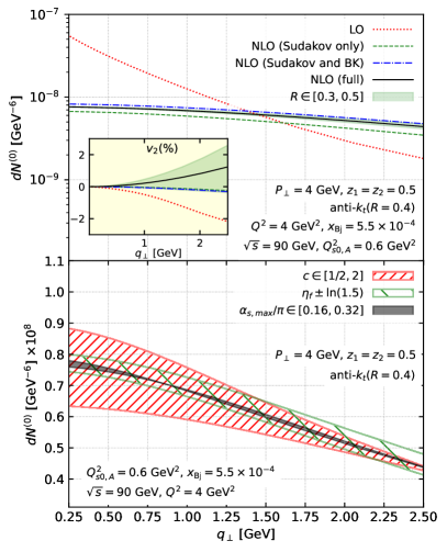
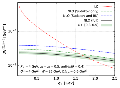
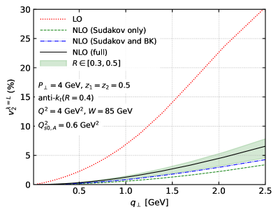
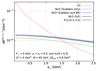
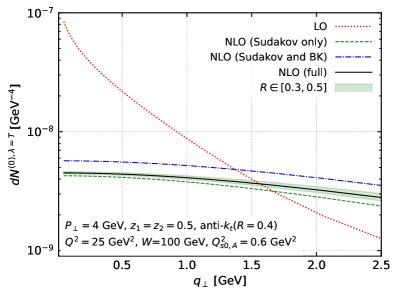
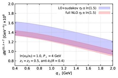
Figure 2: (Top) Azimuthally averaged LO and NLO back-to-back dijet yield as a function of dijet momentum imbalance q ⟂ subscript 𝑞 perpendicular-to q_{\perp} q ⟂ subscript 𝑞 perpendicular-to q_{\perp} v 2 subscript 𝑣 2 v_{2} k t subscript 𝑘 𝑡 k_{t} R = 0.3 − 0.5 𝑅 0.3 0.5 R=0.3-0.5 α s subscript 𝛼 𝑠 \alpha_{s}
Results in EIC kinematics for the azimuthally averaged back-to-back dijet yield versus q ⟂ subscript 𝑞 perpendicular-to q_{\perp} 2 x 𝑥 x q ⟂ ≲ 1.5 less-than-or-similar-to subscript 𝑞 perpendicular-to 1.5 q_{\perp}\lesssim 1.5 x 𝑥 x R 𝑅 R R 𝑅 R
The inset shows the q ⟂ subscript 𝑞 perpendicular-to q_{\perp} v 2 = d σ ( 2 ) / d σ ( 0 ) subscript 𝑣 2 d superscript 𝜎 2 d superscript 𝜎 0 v_{2}=\mathrm{d}\sigma^{(2)}/\mathrm{d}\sigma^{(0)} < 2 % absent percent 2 <2\% v 2 subscript 𝑣 2 v_{2} v 2 subscript 𝑣 2 v_{2} R 𝑅 R v 2 λ = L ∝ h ^ 0 proportional-to superscript subscript 𝑣 2 𝜆 𝐿 superscript ^ ℎ 0 v_{2}^{\lambda=L}\propto\hat{h}^{0} R 𝑅 R
Theory uncertainties in the NLO result can be divided into four classes; three of these are displayed in Fig. 2 2 LO contributions beyond the NLO impact factor; they are estimated by varying the running coupling scale c = 0.5 − 2 𝑐 0.5 2 c=0.5-2 μ R = c P ⟂ subscript 𝜇 𝑅 𝑐 subscript 𝑃 perpendicular-to \mu_{R}=cP_{\perp} α s 2 ln 2 ( P ⟂ / μ 0 ) superscript subscript 𝛼 𝑠 2 superscript 2 subscript 𝑃 perpendicular-to subscript 𝜇 0 \alpha_{s}^{2}\ln^{2}(P_{\perp}/\mu_{0}) q ⟂ subscript 𝑞 perpendicular-to q_{\perp} α s ln ( P ⟂ / μ 0 ) subscript 𝛼 𝑠 subscript 𝑃 perpendicular-to subscript 𝜇 0 \alpha_{s}\ln(P_{\perp}/\mu_{0})
The second source of uncertainty is from
the target-rapidity factorization scale η f subscript 𝜂 𝑓 \eta_{f} x f subscript 𝑥 𝑓 x_{f} x g subscript 𝑥 𝑔 x_{g} q ⟂ ≳ Q s greater-than-or-equivalent-to subscript 𝑞 perpendicular-to subscript 𝑄 𝑠 q_{\perp}\gtrsim Q_{s} α s , max subscript 𝛼 𝑠 max
\alpha_{s,{\rm max}} 2 Q s subscript 𝑄 𝑠 Q_{s} q ⟂ 2 / P ⟂ 2 , Q s 2 / P ⟂ 2 superscript subscript 𝑞 perpendicular-to 2 superscript subscript 𝑃 perpendicular-to 2 superscript subscript 𝑄 𝑠 2 superscript subscript 𝑃 perpendicular-to 2
q_{\perp}^{2}/P_{\perp}^{2},Q_{s}^{2}/P_{\perp}^{2} [28 , 29 ] ,
of 𝒪 ( 10 % ) 𝒪 percent 10 \mathcal{O}(10\%) q ⟂ ≲ 1.5 less-than-or-similar-to subscript 𝑞 perpendicular-to 1.5 q_{\perp}\lesssim 1.5 P ⟂ = 4 subscript 𝑃 perpendicular-to 4 P_{\perp}=4
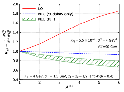
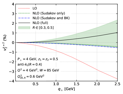
Figure 3: q ⟂ subscript 𝑞 perpendicular-to q_{\perp} A 𝐴 A R e A subscript 𝑅 𝑒 𝐴 R_{eA}
Fig. 3 R e A subscript 𝑅 𝑒 𝐴 R_{eA} q ⟂ subscript 𝑞 perpendicular-to q_{\perp} R e A subscript 𝑅 𝑒 𝐴 R_{eA} A 1 / 3 = 6 superscript 𝐴 1 3 6 A^{1/3}=6 [104 ] ; in the CGC, it is generated by coherent multiple scattering that shifts the typical momentum imbalance to larger q ⟂ subscript 𝑞 perpendicular-to q_{\perp} [105 ] . At NLO, we see that the Cronin enhancement is washed out by Sudakov corrections alone. A further strong effect is seen from the NLO contributions dominantly caused by the WW gluon TMD RGE which suppresses R e A subscript 𝑅 𝑒 𝐴 R_{eA} R p A subscript 𝑅 𝑝 𝐴 R_{pA} [106 , 107 ] .
A qualitative interpretation is that Sudakov logs suppress configurations corresponding to small q ⟂ subscript 𝑞 perpendicular-to q_{\perp} 𝒓 b b ′ subscript 𝒓 𝑏 superscript 𝑏 ′ \boldsymbol{r}_{bb^{\prime}} 𝒓 b b ′ subscript 𝒓 𝑏 superscript 𝑏 ′ \boldsymbol{r}_{bb^{\prime}} x 𝑥 x [108 ] leads to increasing suppression of R e A subscript 𝑅 𝑒 𝐴 R_{eA} A 1 / 3 superscript 𝐴 1 3 A^{1/3} q ⟂ = 1.5 subscript 𝑞 perpendicular-to 1.5 q_{\perp}=1.5 A 1 / 3 superscript 𝐴 1 3 A^{1/3} q ⟂ subscript 𝑞 perpendicular-to q_{\perp}
While more detailed studies are necessary, our results are suggestive that inclusive back-to-back dijets in e+A collisions show strong potential to be a golden channel for gluon saturation at the EIC when combined
with other processes
that constrain the initial condition for the WW small-x 𝑥 x x 𝑥 x [109 , 110 , 111 , 112 , 113 , 114 , 115 , 116 , 117 , 118 , 119 , 120 ] and analogous studies [121 , 122 , 123 , 124 , 125 , 126 , 127 , 128 , 129 , 130 , 131 , 132 , 133 , 134 , 135 , 136 , 137 ] in p+A collisions at RHIC and the LHC will further enable unambiguous determination of the dynamics of gluon saturation.
Acknowledgements. We are grateful to Bertrand Ducloué and Feng Yuan for valuable discussions. P.C., F.S. and T.S. thank the EIC theory institute at BNL for its support during the final stages of this work. F.S. is supported by the National Science Foundation under grant No. PHY-1945471, and the UC Southern California Hub, with funding from the UC National Laboratories division of the University of California Office of the President.
T.S. kindly acknowledges support of the Polish National Science Center (NCN) Grants No. 2019/32/C/ST2/00202 and 2021/43/D/ST2/03375.
B.P.S. and R.V. are supported by the U.S. Department of Energy, Office of Science, Office of Nuclear Physics, under DOE Contract No. DE-SC0012704 and within the framework of the Saturated Glue (SURGE) Topical Theory Collaboration. R.V.’s work is also supported in part by an LDRD grant from Brookhaven Science Associates.
References
Boussarie et al. [2023]
R. Boussarie et al. , (2023), arXiv:2304.03302 [hep-ph]
.
McLerran and Venugopalan [1994a]
L. D. McLerran and R. Venugopalan, Phys. Rev. D 49 , 2233 (1994a) , arXiv:hep-ph/9309289
.
McLerran and Venugopalan [1994b]
L. D. McLerran and R. Venugopalan, Phys. Rev. D49 , 3352 (1994b) , arXiv:hep-ph/9311205 [hep-ph]
.
Kovchegov and Mueller [1998]
Y. V. Kovchegov and A. H. Mueller, Nucl. Phys. B 529 , 451 (1998) , arXiv:hep-ph/9802440 .
Gribov et al. [1983]
L. Gribov, E. Levin, and M. Ryskin, Phys. Rept. 100 , 1 (1983) .
Mueller and Qiu [1986]
A. H. Mueller and J.-w. Qiu, Nucl. Phys. B 268 , 427 (1986) .
Dominguez et al. [2011a]
F. Dominguez, B.-W. Xiao,
and F. Yuan, Phys. Rev. Lett. 106 , 022301 (2011a) , arXiv:1009.2141 [hep-ph] .
Dominguez et al. [2011b]
F. Dominguez, C. Marquet,
B.-W. Xiao, and F. Yuan, Phys.
Rev. D 83 , 105005
(2011b) , arXiv:1101.0715 [hep-ph] .
Catani and Trentadue [1989]
S. Catani and L. Trentadue, Nucl. Phys. B 327 , 323 (1989) .
Catani and Trentadue [1991]
S. Catani and L. Trentadue, Nucl. Phys. B 353 , 183 (1991) .
Catani and Hautmann [1994]
S. Catani and F. Hautmann, Nucl. Phys. B 427 , 475 (1994) , arXiv:hep-ph/9405388 .
Balitsky and Tarasov [2015]
I. Balitsky and A. Tarasov, JHEP 10 , 017 (2015) , arXiv:1505.02151 [hep-ph] .
Balitsky and Chirilli [2022]
I. Balitsky and G. A. Chirilli, Phys. Rev. D 106 , 034007 (2022) , arXiv:2205.03119 [hep-ph] .
Balitsky [2023]
I. Balitsky, JHEP 03 , 029 (2023) , arXiv:2301.01717 [hep-ph] .
Mueller et al. [2013a]
A. H. Mueller, B.-W. Xiao, and F. Yuan, Phys. Rev. Lett. 110 , 082301 (2013a) , arXiv:1210.5792 [hep-ph] .
Mueller et al. [2013b]
A. H. Mueller, B.-W. Xiao, and F. Yuan, Phys. Rev. D 88 , 114010 (2013b) , arXiv:1308.2993 [hep-ph] .
Xiao et al. [2017]
B.-W. Xiao, F. Yuan, and J. Zhou, Nucl. Phys. B 921 , 104
(2017) , arXiv:1703.06163 [hep-ph] .
Gelis and Jalilian-Marian [2003]
F. Gelis and J. Jalilian-Marian, Phys. Rev. D67 , 074019 (2003) , arXiv:hep-ph/0211363 [hep-ph]
.
Albacete and Marquet [2014]
J. L. Albacete and C. Marquet, Prog. Part. Nucl. Phys. 76 , 1 (2014) , arXiv:1401.4866 [hep-ph] .
Morreale and Salazar [2021]
A. Morreale and F. Salazar, Universe 7 , 312 (2021) , arXiv:2108.08254 [hep-ph] .
Note [1]
A detailed derivation of the cross-section for
longitudinally polarized virtual photons is provided in a previous
paper [49 ] .
Accardi et al. [2016]
A. Accardi et al. , Eur. Phys. J. A 52 , 268 (2016) , arXiv:1212.1701 [nucl-ex]
.
Aschenauer et al. [2019]
E. C. Aschenauer, S. Fazio,
J. H. Lee, H. Mäntysaari, B. S. Page, B. Schenke, T. Ullrich, R. Venugopalan, and P. Zurita, Rept. Prog. Phys. 82 , 024301 (2019) , arXiv:1708.01527
[nucl-ex] .
Abdul Khalek et al. [2022]
R. Abdul Khalek et al. , Nucl. Phys. A 1026 , 122447 (2022) , arXiv:2103.05419 [physics.ins-det]
.
Dumitru and Skokov [2015]
A. Dumitru and V. Skokov, Phys. Rev. D 91 , 074006 (2015) , arXiv:1411.6630 [hep-ph] .
Dumitru et al. [2019]
A. Dumitru, V. Skokov, and T. Ullrich, Phys. Rev. C 99 , 015204 (2019) , arXiv:1809.02615 [hep-ph] .
Zhao et al. [2021]
Y.-Y. Zhao, M.-M. Xu,
L.-Z. Chen, D.-H. Zhang, and Y.-F. Wu, Phys. Rev. D 104 , 114032 (2021) , arXiv:2105.08818 [hep-ph] .
Mäntysaari et al. [2020]
H. Mäntysaari, N. Mueller, F. Salazar, and B. Schenke, Phys. Rev. Lett. 124 , 112301 (2020) , arXiv:1912.05586 [nucl-th] .
Boussarie et al. [2021]
R. Boussarie, H. Mäntysaari, F. Salazar, and B. Schenke, JHEP 09 , 178 (2021) , arXiv:2106.11301 [hep-ph] .
van Hameren et al. [2021]
A. van
Hameren, P. Kotko,
K. Kutak, S. Sapeta, and E. Żarów, Eur. Phys. J. C 81 , 741
(2021) , arXiv:2106.13964 [hep-ph] .
Zheng et al. [2014]
L. Zheng, E. C. Aschenauer, J. H. Lee,
and B.-W. Xiao, PoS DIS2014 , 255 (2014) .
Bergabo and Jalilian-Marian [2023a]
F. Bergabo and J. Jalilian-Marian, Phys. Rev. D 107 , 054036 (2023a) , arXiv:2301.03117 [hep-ph]
.
Caucal et al. [2021]
P. Caucal, F. Salazar, and R. Venugopalan, JHEP 11 , 222
(2021) , arXiv:2108.06347 [hep-ph] .
Balitsky [1996]
I. Balitsky, Nucl. Phys. B 463 , 99 (1996) , arXiv:hep-ph/9509348 .
Jalilian-Marian et al. [1997]
J. Jalilian-Marian, A. Kovner, L. D. McLerran, and H. Weigert, Phys. Rev. D 55 , 5414 (1997) , arXiv:hep-ph/9606337 .
Jalilian-Marian et al. [1998]
J. Jalilian-Marian, A. Kovner, and H. Weigert, Phys. Rev. D 59 , 014015 (1998) , arXiv:hep-ph/9709432 .
Kovner et al. [2000]
A. Kovner, J. G. Milhano,
and H. Weigert, Phys. Rev. D 62 , 114005 (2000) , arXiv:hep-ph/0004014 .
Iancu et al. [2001a]
E. Iancu, A. Leonidov, and L. D. McLerran, Nucl. Phys. A 692 , 583 (2001a) , arXiv:hep-ph/0011241 .
Iancu et al. [2001b]
E. Iancu, A. Leonidov, and L. D. McLerran, Phys. Lett. B 510 , 133 (2001b) , arXiv:hep-ph/0102009 .
Ferreiro et al. [2002]
E. Ferreiro, E. Iancu,
A. Leonidov, and L. McLerran, Nucl. Phys. A 703 , 489 (2002) , arXiv:hep-ph/0109115 .
Note [2]
We use the words projectile rapidity for Y = l n ( k − / q − ) 𝑌 𝑙 𝑛 superscript 𝑘 superscript 𝑞 Y=\mathop{ln}\nolimits(k^{-}/q^{-}) η = l n ( P + / k + ) 𝜂 𝑙 𝑛 superscript 𝑃 superscript 𝑘 \eta=\mathop{ln}\nolimits(P^{+}/k^{+}) y = 1 / 2 l n ( k + / k − ) 𝑦 1 2 𝑙 𝑛 superscript 𝑘 superscript 𝑘 y=1/2\mathop{ln}\nolimits(k^{+}/k^{-}) y = y γ ∗ − 1 / 2 ( l n ( x Bj ) + Y + η ) 𝑦 subscript 𝑦 superscript 𝛾 1 2 𝑙 𝑛 subscript 𝑥 Bj 𝑌 𝜂 y=y_{\gamma^{*}}-1/2(\mathop{ln}\nolimits(x_{\rm Bj})+Y+\eta) y γ ∗ subscript 𝑦 superscript 𝛾 y_{\gamma^{*}}
Balitsky and Chirilli [2013]
I. Balitsky and G. A. Chirilli, Phys. Rev. D88 , 111501 (2013) , arXiv:1309.7644 [hep-ph] .
Kovner et al. [2014a]
A. Kovner, M. Lublinsky, and Y. Mulian, Phys. Rev. D89 , 061704 (2014a) , arXiv:1310.0378 [hep-ph] .
Kovner et al. [2014b]
A. Kovner, M. Lublinsky, and Y. Mulian, JHEP 08 , 114 (2014b) , arXiv:1405.0418 [hep-ph] .
Lublinsky and Mulian [2017]
M. Lublinsky and Y. Mulian, JHEP 05 , 097 (2017) , arXiv:1610.03453 [hep-ph] .
Altinoluk and Boussarie [2019]
T. Altinoluk and R. Boussarie, JHEP 10 , 208 (2019) , arXiv:1902.07930 [hep-ph] .
Boussarie and Mehtar-Tani [2021]
R. Boussarie and Y. Mehtar-Tani, Phys. Rev. D 103 , 094012 (2021) , arXiv:2001.06449 [hep-ph] .
Rodriguez-Aguilar et al. [2023]
B. Rodriguez-Aguilar, D. N. Triantafyllopoulos, and S. Y. Wei, Phys. Rev. D 107 , 114007 (2023) , arXiv:2302.01106 [hep-ph]
.
Caucal et al. [2023]
P. Caucal, F. Salazar,
B. Schenke, T. Stebel, and R. Venugopalan, JHEP 08 , 062 (2023) , arXiv:2304.03304
[hep-ph] .
Caucal et al. [2022]
P. Caucal, F. Salazar,
B. Schenke, and R. Venugopalan, JHEP 11 , 169 (2022) , arXiv:2208.13872
[hep-ph] .
Taels et al. [2022]
P. Taels, T. Altinoluk,
G. Beuf, and C. Marquet, JHEP 10 , 184 (2022) , arXiv:2204.11650
[hep-ph] .
Gribov et al. [1965]
V. N. Gribov, B. L. Ioffe, and I. Y. Pomeranchuk, Yad. Fiz. 2 , 768 (1965).
Ioffe [1969]
B. L. Ioffe, Phys. Lett. B 30 , 123 (1969) .
Andersson et al. [1996]
B. Andersson, G. Gustafson, and J. Samuelsson, Nucl. Phys. B 467 , 443 (1996) .
Kwiecinski et al. [1996]
J. Kwiecinski, A. D. Martin, and P. J. Sutton, Z. Phys. C 71 , 585 (1996) , arXiv:hep-ph/9602320 .
Kwiecinski et al. [1997]
J. Kwiecinski, A. D. Martin, and A. M. Stasto, Phys. Rev. D 56 , 3991 (1997) , arXiv:hep-ph/9703445 .
Salam [1998]
G. P. Salam, JHEP 07 , 019 (1998) , arXiv:hep-ph/9806482 .
Ciafaloni and Colferai [1999]
M. Ciafaloni and D. Colferai, Phys. Lett. B 452 , 372 (1999) , arXiv:hep-ph/9812366 .
Ciafaloni et al. [1999]
M. Ciafaloni, D. Colferai,
and G. P. Salam, Phys. Rev. D 60 , 114036 (1999) , arXiv:hep-ph/9905566 .
Ciafaloni et al. [2003]
M. Ciafaloni, D. Colferai,
G. P. Salam, and A. M. Stasto, Phys. Rev. D 68 , 114003 (2003) , arXiv:hep-ph/0307188 .
Sabio Vera [2005]
A. Sabio Vera, Nucl. Phys. B 722 , 65 (2005) , arXiv:hep-ph/0505128 .
Motyka and Stasto [2009]
L. Motyka and A. M. Stasto, Phys. Rev. D 79 , 085016 (2009) , arXiv:0901.4949 [hep-ph] .
Beuf [2014]
G. Beuf, Phys. Rev. D 89 , 074039 (2014) , arXiv:1401.0313 [hep-ph] .
Iancu et al. [2015a]
E. Iancu, J. Madrigal,
A. Mueller, G. Soyez, and D. Triantafyllopoulos, Phys. Lett. B 744 , 293
(2015a) , arXiv:1502.05642 [hep-ph] .
Hatta and Iancu [2016]
Y. Hatta and E. Iancu, JHEP 08 , 083
(2016) , arXiv:1606.03269 [hep-ph] .
Ducloué et al. [2019]
B. Ducloué, E. Iancu,
A. Mueller, G. Soyez, and D. Triantafyllopoulos, JHEP 04 , 081 (2019) , arXiv:1902.06637
[hep-ph] .
Ducloué et al. [2020]
B. Ducloué, E. Iancu,
G. Soyez, and D. N. Triantafyllopoulos, Phys. Lett. B 803 , 135305 (2020) , arXiv:1912.09196 [hep-ph] .
Dominguez et al. [2012]
F. Dominguez, J.-W. Qiu,
B.-W. Xiao, and F. Yuan, Phys.
Rev. D 85 , 045003
(2012) , arXiv:1109.6293 [hep-ph] .
Hatta et al. [2021a]
Y. Hatta, B.-W. Xiao,
F. Yuan, and J. Zhou, Phys. Rev. Lett. 126 , 142001 (2021a) , arXiv:2010.10774 [hep-ph] .
Hatta et al. [2021b]
Y. Hatta, B.-W. Xiao,
F. Yuan, and J. Zhou, Phys. Rev. D 104 , 054037 (2021b) , arXiv:2106.05307 [hep-ph] .
Cacciari et al. [2008]
M. Cacciari, G. P. Salam,
and G. Soyez, JHEP 04 , 063
(2008) , arXiv:0802.1189 [hep-ph] .
Ayala et al. [1996]
A. Ayala, J. Jalilian-Marian, L. D. McLerran, and R. Venugopalan, Phys. Rev. D 53 , 458 (1996) , arXiv:hep-ph/9508302 .
Zhou [2019]
J. Zhou, Phys. Rev. D 99 , 054026 (2019) , arXiv:1807.00506 [hep-ph] .
Dokshitzer et al. [1997]
Y. L. Dokshitzer, G. D. Leder, S. Moretti, and B. R. Webber, JHEP 08 , 001 (1997) , arXiv:hep-ph/9707323 .
Wobisch and Wengler [1998]
M. Wobisch and T. Wengler, in Workshop on
Monte Carlo Generators for HERA Physics (Plenary Starting Meeting) (1998) pp. 270–279, arXiv:hep-ph/9907280 .
Salam [2010]
G. P. Salam, Eur. Phys. J. C 67 , 637 (2010) , arXiv:0906.1833 [hep-ph] .
Cacciari et al. [2012]
M. Cacciari, G. P. Salam,
and G. Soyez, Eur. Phys. J. C 72 , 1896 (2012) , arXiv:1111.6097 [hep-ph] .
Salam and Soyez [2007]
G. P. Salam and G. Soyez, JHEP 05 , 086 (2007) , arXiv:0704.0292 [hep-ph] .
Ivanov and Papa [2012a]
D. Y. Ivanov and A. Papa, JHEP 05 , 086
(2012a) , arXiv:1202.1082 [hep-ph] .
Kang et al. [2017]
Z.-B. Kang, F. Ringer, and W. J. Waalewijn, JHEP 07 , 064 (2017) , arXiv:1705.05375
[hep-ph] .
Abramowitz and Stegun [1964]
M. Abramowitz and I. A. Stegun, Handbook of mathematical
functions with formulas, graphs, and mathematical tables , Vol. 55 (US Government printing office, 1964).
Cali et al. [2021]
S. Cali, K. Cichy,
P. Korcyl, P. Kotko, K. Kutak, and C. Marquet, Eur. Phys. J. C 81 , 663
(2021) , arXiv:2104.14254 [hep-ph] .
Dominguez et al. [2011c]
F. Dominguez, A. H. Mueller, S. Munier, and B.-W. Xiao, Phys. Lett. B 705 , 106 (2011c) , arXiv:1108.1752 [hep-ph] .
Kang et al. [2021]
Z.-B. Kang, J. Reiten,
D. Y. Shao, and J. Terry, JHEP 05 , 286 (2021) , arXiv:2012.01756
[hep-ph] .
del Castillo et al. [2021]
R. F. del Castillo, M. G. Echevarria, Y. Makris,
and I. Scimemi, JHEP 01 , 088 (2021) , arXiv:2008.07531
[hep-ph] .
Gao et al. [2023]
M.-S. Gao, Z.-B. Kang,
D. Y. Shao, J. Terry, and C. Zhang, (2023), arXiv:2306.09317
[hep-ph] .
Collins and Soper [1981]
J. C. Collins and D. E. Soper, Nucl. Phys. B 193 , 381 (1981) , [Erratum: Nucl.Phys.B 213, 545 (1983)].
Collins and Soper [1982]
J. C. Collins and D. E. Soper, Nucl. Phys. B 194 , 445 (1982) .
Collins et al. [1985]
J. C. Collins, D. E. Soper,
and G. F. Sterman, Nucl. Phys. B 250 , 199 (1985) .
Blaizot et al. [2004]
J. P. Blaizot, F. Gelis, and R. Venugopalan, Nucl. Phys. A 743 , 57 (2004) , arXiv:hep-ph/0402257 .
Dumitru et al. [2011]
A. Dumitru, J. Jalilian-Marian, T. Lappi, B. Schenke, and R. Venugopalan, Phys. Lett. B 706 , 219 (2011) , arXiv:1108.4764 [hep-ph] .
Iancu and Triantafyllopoulos [2012]
E. Iancu and D. N. Triantafyllopoulos, JHEP 04 , 025 (2012) , arXiv:1112.1104 [hep-ph] .
Metz and Zhou [2011]
A. Metz and J. Zhou, Phys. Rev. D 84 , 051503 (2011) , arXiv:1105.1991 [hep-ph] .
Kovchegov [1999]
Y. V. Kovchegov, Phys. Rev. D 60 , 034008 (1999) , arXiv:hep-ph/9901281 .
Note [3]
The validity of this approximation relative to the full LL
JIMWLK RGE was explored in [91 ] and shown to be quite good
for a range of spatial configurations of dipoles.
Kowalski et al. [2008]
H. Kowalski, T. Lappi, and R. Venugopalan, Phys. Rev. Lett. 100 , 022303 (2008) , arXiv:0705.3047 [hep-ph] .
Lappi and Mäntysaari [2013]
T. Lappi and H. Mäntysaari, Phys. Rev. D 88 , 114020 (2013) , arXiv:1309.6963 [hep-ph] .
Aaron et al. [2010]
F. D. Aaron et al. (H1, ZEUS), JHEP 01 , 109 (2010) , arXiv:0911.0884
[hep-ex] .
Balitsky and Chirilli [2008]
I. Balitsky and G. A. Chirilli, Phys. Rev. D 77 , 014019 (2008) , arXiv:0710.4330 [hep-ph] .
Lappi and Mäntysaari [2015]
T. Lappi and H. Mäntysaari, Phys. Rev. D 91 , 074016 (2015) , arXiv:1502.02400 [hep-ph] .
Lappi and Mäntysaari [2016]
T. Lappi and H. Mäntysaari, Phys. Rev. D 93 , 094004 (2016) , arXiv:1601.06598 [hep-ph] .
Kovchegov and Weigert [2007]
Y. V. Kovchegov and H. Weigert, Nucl. Phys. A784 , 188 (2007) , arXiv:hep-ph/0609090 [hep-ph]
.
Iancu et al. [2015b]
E. Iancu, J. D. Madrigal,
A. H. Mueller, G. Soyez, and D. N. Triantafyllopoulos, Phys. Lett. B 750 , 643
(2015b) , arXiv:1507.03651 [hep-ph] .
Antreasyan et al. [1979]
D. Antreasyan, J. W. Cronin, H. J. Frisch,
M. J. Shochet, L. Kluberg, P. A. Piroue, and R. L. Sumner, Phys.
Rev. D 19 , 764 (1979) .
Jalilian-Marian et al. [2003]
J. Jalilian-Marian, Y. Nara, and R. Venugopalan, Phys. Lett. B 577 , 54 (2003) , arXiv:nucl-th/0307022 .
Kharzeev et al. [2003]
D. Kharzeev, Y. V. Kovchegov, and K. Tuchin, Phys. Rev. D 68 , 094013 (2003) , arXiv:hep-ph/0307037 .
Albacete et al. [2004]
J. L. Albacete, N. Armesto,
A. Kovner, C. A. Salgado, and U. A. Wiedemann, Phys. Rev. Lett. 92 , 082001 (2004) , arXiv:hep-ph/0307179 .
Mueller [2003]
A. H. Mueller, Nucl. Phys. A 724 , 223 (2003) , arXiv:hep-ph/0301109 .
Boussarie et al. [2017]
R. Boussarie, A. V. Grabovsky, D. Yu. Ivanov, L. Szymanowski, and S. Wallon, Phys. Rev. Lett. 119 , 072002 (2017) , arXiv:1612.08026 [hep-ph]
.
Boussarie et al. [2016]
R. Boussarie, A. V. Grabovsky, L. Szymanowski, and S. Wallon, JHEP 11 , 149 (2016) , arXiv:1606.00419 [hep-ph] .
Roy and Venugopalan [2020a]
K. Roy and R. Venugopalan, Phys. Rev. D 101 , 071505 (2020a) , arXiv:1911.04519 [hep-ph]
.
Roy and Venugopalan [2020b]
K. Roy and R. Venugopalan, Phys. Rev. D 101 , 034028 (2020b) , arXiv:1911.04530 [hep-ph]
.
Beuf et al. [2020]
G. Beuf, H. Hänninen,
T. Lappi, and H. Mäntysaari, Phys. Rev. D 102 , 074028 (2020) , arXiv:2007.01645 [hep-ph] .
Beuf et al. [2022a]
G. Beuf, T. Lappi, and R. Paatelainen, Phys. Rev. Lett. 129 , 072001 (2022a) , arXiv:2112.03158 [hep-ph] .
Mäntysaari and Penttala [2022]
H. Mäntysaari and J. Penttala, JHEP 08 , 247 (2022) , arXiv:2204.14031 [hep-ph] .
Bergabo and Jalilian-Marian [2023b]
F. Bergabo and J. Jalilian-Marian, JHEP 01 , 095 (2023b) , arXiv:2210.03208 [hep-ph] .
Beuf et al. [2022b]
G. Beuf, H. Hänninen,
T. Lappi, Y. Mulian, and H. Mäntysaari, Phys. Rev. D 106 , 094014 (2022b) , arXiv:2206.13161 [hep-ph] .
Tong et al. [2023]
X.-B. Tong, B.-W. Xiao, and Y.-Y. Zhang, Phys. Rev. Lett. 130 , 151902 (2023) , arXiv:2211.01647 [hep-ph] .
Fucilla et al. [2023]
M. Fucilla, A. V. Grabovsky, E. Li,
L. Szymanowski, and S. Wallon, JHEP 03 , 159 (2023) , arXiv:2211.05774
[hep-ph] .
Lipatov and Malyshev [2023]
A. V. Lipatov and M. A. Malyshev, Phys. Rev. D 108 , 014022 (2023) , arXiv:2305.04005 [hep-ph] .
Chirilli et al. [2012]
G. A. Chirilli, B.-W. Xiao,
and F. Yuan, Phys. Rev. Lett. 108 , 122301 (2012) , arXiv:1112.1061 [hep-ph] .
Ivanov and Papa [2012b]
D. Y. Ivanov and A. Papa, JHEP 07 , 045
(2012b) , arXiv:1205.6068 [hep-ph] .
Altinoluk et al. [2015]
T. Altinoluk, N. Armesto,
G. Beuf, A. Kovner, and M. Lublinsky, Phys.
Rev. D 91 , 094016
(2015) , arXiv:1411.2869 [hep-ph] .
Celiberto et al. [2017]
F. G. Celiberto, D. Y. Ivanov, B. Murdaca, and A. Papa, Eur. Phys. J. C 77 , 382 (2017) , arXiv:1701.05077 [hep-ph] .
Stasto et al. [2018]
A. Stasto, S.-Y. Wei,
B.-W. Xiao, and F. Yuan, Phys. Lett. B 784 , 301
(2018) , arXiv:1805.05712 [hep-ph] .
Albacete et al. [2019]
J. L. Albacete, G. Giacalone,
C. Marquet, and M. Matas, Phys. Rev. D 99 , 014002 (2019) , arXiv:1805.05711 [hep-ph] .
Liu et al. [2020]
H.-Y. Liu, Z.-B. Kang, and X. Liu, Phys. Rev. D 102 , 051502 (2020) , arXiv:2004.11990 [hep-ph] .
Shi et al. [2022]
Y. Shi, L. Wang, S.-Y. Wei, and B.-W. Xiao, Phys. Rev. Lett. 128 , 202302 (2022) , arXiv:2112.06975 [hep-ph] .
Hentschinski [2021]
M. Hentschinski, Phys. Rev. D 104 , 054014 (2021) , arXiv:2107.06203 [hep-ph] .
Liu et al. [2022]
H.-y. Liu, K. Xie, Z. Kang, and X. Liu, JHEP 07 , 041 (2022) , arXiv:2204.03026
[hep-ph] .
Wang et al. [2023]
L. Wang, L. Chen, Z. Gao, Y. Shi, S.-Y. Wei, and B.-W. Xiao, Phys. Rev. D 107 , 016016 (2023) , arXiv:2211.08322 [hep-ph]
.
van Hameren et al. [2022]
A. van
Hameren, L. Motyka, and G. Ziarko, JHEP 11 , 103 (2022) , arXiv:2205.09585
[hep-ph] .
Hentschinski et al. [2021]
M. Hentschinski, K. Kutak,
and A. van Hameren, Eur. Phys. J. C 81 , 112 (2021) , [Erratum:
Eur.Phys.J.C 81, 262 (2021)], arXiv:2011.03193 [hep-ph] .
Celiberto et al. [2022]
F. G. Celiberto, M. Fucilla,
D. Y. Ivanov, M. M. A. Mohammed, and A. Papa, JHEP 08 , 092 (2022) , arXiv:2205.02681
[hep-ph] .
van Hameren et al. [2023]
A. van
Hameren, H. Kakkad,
P. Kotko, K. Kutak, and S. Sapeta, (2023), arXiv:2306.17513
[hep-ph] .
Ganguli et al. [2023]
I. Ganguli, A. van
Hameren, P. Kotko, and K. Kutak, (2023), arXiv:2306.04706 [hep-ph] .
Altinoluk et al. [2023]
T. Altinoluk, N. Armesto,
A. Kovner, and M. Lublinsky, (2023), arXiv:2307.14922 [hep-ph] .
Appendix B Supplemental Material 1: Summary of analytic results for the NLO coefficient functions
The inclusive back-to-back dijet differential cross-section in DIS is decomposed according to the virtual photon polarization (longitudinal or transverse):
d σ e + A → e ′ + q q ¯ + X d x Bj d Q 2 d 2 𝑷 ⟂ d 2 𝒒 ⟂ d η 1 d η 2 = ∑ λ = L , T ϕ λ ( x Bj , Q 2 ) d σ γ λ ∗ + A → q q ¯ + X d 2 𝑷 ⟂ d 2 𝒒 ⟂ d η 1 d η 2 | η f , d superscript 𝜎 → 𝑒 𝐴 superscript 𝑒 ′ 𝑞 ¯ 𝑞 𝑋 d subscript 𝑥 Bj d superscript 𝑄 2 superscript d 2 subscript 𝑷 perpendicular-to superscript d 2 subscript 𝒒 perpendicular-to d subscript 𝜂 1 d subscript 𝜂 2 evaluated-at subscript 𝜆 L T
subscript italic-ϕ 𝜆 subscript 𝑥 Bj superscript 𝑄 2 d superscript 𝜎 → superscript subscript 𝛾 𝜆 𝐴 𝑞 ¯ 𝑞 𝑋 superscript d 2 subscript 𝑷 perpendicular-to superscript d 2 subscript 𝒒 perpendicular-to d subscript 𝜂 1 d subscript 𝜂 2 subscript 𝜂 𝑓 \frac{\mathrm{d}\sigma^{e+A\to e^{\prime}+q\bar{q}+X}}{\mathrm{d}x_{\rm Bj}\mathrm{d}Q^{2}\mathrm{d}^{2}\boldsymbol{P}_{\perp}\mathrm{d}^{2}\boldsymbol{q}_{\perp}\mathrm{d}\eta_{1}\mathrm{d}\eta_{2}}=\sum_{\lambda=\mathrm{L,T}}\phi_{\lambda}(x_{\rm Bj},Q^{2})\ \left.\frac{\mathrm{d}\sigma^{\gamma_{\lambda}^{*}+A\to q\bar{q}+X}}{\mathrm{d}^{2}\boldsymbol{P}_{\perp}\mathrm{d}^{2}\boldsymbol{q}_{\perp}\mathrm{d}\eta_{1}\mathrm{d}\eta_{2}}\right|_{\eta_{f}}\,, (14)
with the photon flux factors ϕ λ subscript italic-ϕ 𝜆 \phi_{\lambda}
ϕ λ = L ( x Bj , Q 2 ) subscript italic-ϕ 𝜆 L subscript 𝑥 Bj superscript 𝑄 2 \displaystyle\phi_{\lambda=\mathrm{L}}(x_{\rm Bj},Q^{2}) = α em π Q 2 x Bj ( 1 − y ) , absent subscript 𝛼 em 𝜋 superscript 𝑄 2 subscript 𝑥 Bj 1 𝑦 \displaystyle=\frac{\alpha_{\mathrm{em}}}{\pi Q^{2}x_{\rm Bj}}(1-y)\,, (15)
ϕ λ = T ( x Bj , Q 2 ) subscript italic-ϕ 𝜆 T subscript 𝑥 Bj superscript 𝑄 2 \displaystyle\phi_{\lambda=\mathrm{T}}(x_{\rm Bj},Q^{2}) = α em 2 π Q 2 x Bj [ 1 + ( 1 − y ) 2 ] , absent subscript 𝛼 em 2 𝜋 superscript 𝑄 2 subscript 𝑥 Bj delimited-[] 1 superscript 1 𝑦 2 \displaystyle=\frac{\alpha_{\mathrm{em}}}{2\pi Q^{2}x_{\rm Bj}}[1+(1-y)^{2}]\,, (16)
where y 𝑦 y y x Bj = Q 2 / s 𝑦 subscript 𝑥 Bj superscript 𝑄 2 𝑠 y\,x_{\mathrm{Bj}}=Q^{2}/s γ λ ∗ + A → q q ¯ + X → superscript subscript 𝛾 𝜆 𝐴 𝑞 ¯ 𝑞 𝑋 \gamma_{\lambda}^{*}+A\to q\bar{q}+X η f = ln ( 1 / x f ) subscript 𝜂 𝑓 1 subscript 𝑥 𝑓 \eta_{f}=\ln(1/x_{f}) η f ≤ η c = ln ( 1 / x c ) subscript 𝜂 𝑓 subscript 𝜂 𝑐 1 subscript 𝑥 𝑐 \eta_{f}\leq\eta_{c}=\ln(1/x_{c})
x c = 1 e c 0 2 M q q ¯ 2 + Q 2 W 2 + Q 2 . subscript 𝑥 𝑐 1 𝑒 superscript subscript 𝑐 0 2 superscript subscript 𝑀 𝑞 ¯ 𝑞 2 superscript 𝑄 2 superscript 𝑊 2 superscript 𝑄 2 x_{c}=\frac{1}{ec_{0}^{2}}\frac{M_{q\bar{q}}^{2}+Q^{2}}{W^{2}+Q^{2}}\,. (17)
A typical choice for x f subscript 𝑥 𝑓 x_{f} x g = e c 0 2 x c subscript 𝑥 𝑔 𝑒 superscript subscript 𝑐 0 2 subscript 𝑥 𝑐 x_{g}=ec_{0}^{2}x_{c} γ ∗ + g → q + q ¯ → superscript 𝛾 𝑔 𝑞 ¯ 𝑞 \gamma^{*}+g\to q+\bar{q}
As is customary, we decompose the hadronic component of the differential cross-section into Fourier modes in the angle ϕ italic-ϕ \phi 𝑷 ⟂ subscript 𝑷 perpendicular-to \boldsymbol{P}_{\perp} 𝒒 ⟂ subscript 𝒒 perpendicular-to \boldsymbol{q}_{\perp}
d σ γ λ ∗ + A → q q ¯ + X d 2 𝑷 ⟂ d 2 𝒒 ⟂ d η 1 d η 2 | η f = d σ ( 0 ) , λ + 2 ∑ n = 1 ∞ cos ( 2 n ϕ ) d σ ( 2 n ) , λ . evaluated-at d superscript 𝜎 → superscript subscript 𝛾 𝜆 𝐴 𝑞 ¯ 𝑞 𝑋 superscript d 2 subscript 𝑷 perpendicular-to superscript d 2 subscript 𝒒 perpendicular-to d subscript 𝜂 1 d subscript 𝜂 2 subscript 𝜂 𝑓 d superscript 𝜎 0 𝜆
2 superscript subscript 𝑛 1 2 𝑛 italic-ϕ d superscript 𝜎 2 𝑛 𝜆
\displaystyle\left.\frac{\mathrm{d}\sigma^{\gamma_{\lambda}^{*}+A\to q\bar{q}+X}}{\mathrm{d}^{2}\boldsymbol{P}_{\perp}\mathrm{d}^{2}\boldsymbol{q}_{\perp}\mathrm{d}\eta_{1}\mathrm{d}\eta_{2}}\right|_{\eta_{f}}=\mathrm{d}\sigma^{(0),\lambda}+2\sum_{n=1}^{\infty}\cos(2n\phi)\mathrm{d}\sigma^{(2n),\lambda}\,. (18)
We present results both for longitudinally and transversely polarized photons. The leading order hard factors are
ℋ LO λ = L , i j = α em e f 2 α s δ ( 1 − z 1 − z 2 ) 16 z 1 3 z 2 3 Q 2 𝑷 ⟂ i 𝑷 ⟂ j ( 𝑷 ⟂ 2 + z 1 z 2 Q 2 ) 4 , superscript subscript ℋ LO 𝜆 L 𝑖 𝑗
subscript 𝛼 em superscript subscript 𝑒 𝑓 2 subscript 𝛼 𝑠 𝛿 1 subscript 𝑧 1 subscript 𝑧 2 16 superscript subscript 𝑧 1 3 superscript subscript 𝑧 2 3 superscript 𝑄 2 superscript subscript 𝑷 perpendicular-to 𝑖 superscript subscript 𝑷 perpendicular-to 𝑗 superscript superscript subscript 𝑷 perpendicular-to 2 subscript 𝑧 1 subscript 𝑧 2 superscript 𝑄 2 4 \displaystyle\mathcal{H}_{\rm LO}^{\lambda=\textrm{L},ij}=\alpha_{\rm em}e_{f}^{2}\alpha_{s}\delta(1-z_{1}-z_{2})16\,z_{1}^{3}z_{2}^{3}\,Q^{2}\,\frac{\boldsymbol{P}_{\perp}^{i}\boldsymbol{P}_{\perp}^{j}}{(\boldsymbol{P}_{\perp}^{2}+z_{1}z_{2}Q^{2})^{4}}\,, (19)
ℋ LO λ = T , i j superscript subscript ℋ LO 𝜆 T 𝑖 𝑗
\displaystyle\mathcal{H}_{\rm LO}^{\lambda=\textrm{T},ij} = α em e f 2 α s δ ( 1 − z 1 − z 2 ) z 1 z 2 ( z 1 2 + z 2 2 ) [ δ i j ( 𝑷 ⟂ 2 + z 1 z 2 Q 2 ) 2 − 4 z 1 z 2 Q 2 𝑷 ⟂ i 𝑷 ⟂ j ( 𝑷 ⟂ 2 + z 1 z 2 Q 2 ) 4 ] , absent subscript 𝛼 em superscript subscript 𝑒 𝑓 2 subscript 𝛼 𝑠 𝛿 1 subscript 𝑧 1 subscript 𝑧 2 subscript 𝑧 1 subscript 𝑧 2 superscript subscript 𝑧 1 2 superscript subscript 𝑧 2 2 delimited-[] superscript 𝛿 𝑖 𝑗 superscript superscript subscript 𝑷 perpendicular-to 2 subscript 𝑧 1 subscript 𝑧 2 superscript 𝑄 2 2 4 subscript 𝑧 1 subscript 𝑧 2 superscript 𝑄 2 superscript subscript 𝑷 perpendicular-to 𝑖 superscript subscript 𝑷 perpendicular-to 𝑗 superscript superscript subscript 𝑷 perpendicular-to 2 subscript 𝑧 1 subscript 𝑧 2 superscript 𝑄 2 4 \displaystyle=\alpha_{\rm em}e_{f}^{2}\alpha_{s}\delta(1-z_{1}-z_{2})z_{1}z_{2}(z_{1}^{2}+z_{2}^{2})\left[\frac{\delta^{ij}}{(\boldsymbol{P}_{\perp}^{2}+z_{1}z_{2}Q^{2})^{2}}-\frac{4z_{1}z_{2}Q^{2}\boldsymbol{P}_{\perp}^{i}\boldsymbol{P}_{\perp}^{j}}{(\boldsymbol{P}_{\perp}^{2}+z_{1}z_{2}Q^{2})^{4}}\right]\,, (20)
for transversely and longitudinally polarized photons respectively. Here α em subscript 𝛼 em \alpha_{\rm em} e f 2 superscript subscript 𝑒 𝑓 2 e_{f}^{2} i , j = 1 , 2 formulae-sequence 𝑖 𝑗
1 2 i,j=1,2
ℋ LO 0 , λ = 1 2 δ i j ℋ LO λ , i j . superscript subscript ℋ LO 0 𝜆
1 2 superscript 𝛿 𝑖 𝑗 superscript subscript ℋ LO 𝜆 𝑖 𝑗
\displaystyle\mathcal{H}_{\rm LO}^{0,\lambda}=\frac{1}{2}\delta^{ij}\mathcal{H}_{\rm LO}^{\lambda,ij}\,. (21)
At NLO, for longitudinal photons, the calculation has been detailed in [49 ] . With respect to Eqs. (5.2)-(5.3) in this paper, the only modification to the NLO coefficient function comes from the matching with η 𝜂 \eta Y f = ln ( z f ) subscript 𝑌 𝑓 subscript 𝑧 𝑓 Y_{f}=\ln(z_{f}) 59 − ln ( 𝑷 ⟂ 2 𝒓 b b ′ 2 / c 0 2 ) superscript subscript 𝑷 perpendicular-to 2 superscript subscript 𝒓 𝑏 superscript 𝑏 ′ 2 superscript subscript 𝑐 0 2 -\ln(\boldsymbol{P}_{\perp}^{2}\boldsymbol{r}_{bb^{\prime}}^{2}/c_{0}^{2}) 60
For transversely polarized photons, we combine the results obtained in Supplemental Material 4. More precisely, starting from Eq. (71 ℋ NLO , 1 λ = T superscript subscript ℋ NLO 1
𝜆 T \mathcal{H}_{\rm NLO,1}^{\lambda=\textrm{T}} ℋ NLO , 2 λ = T superscript subscript ℋ NLO 2
𝜆 T \mathcal{H}_{\rm NLO,2}^{\lambda=\textrm{T}} 81 91 92 137 138 139 d σ other ( 0 ) , λ = T d subscript superscript 𝜎 0 𝜆
T other \mathrm{d}\sigma^{(0),\lambda=\rm T}_{\rm other} 145 152 154 160 162 174 177 z g subscript 𝑧 𝑔 z_{g} z g → 0 → subscript 𝑧 𝑔 0 z_{g}\to 0 180 189 Y f = ln ( z f ) subscript 𝑌 𝑓 subscript 𝑧 𝑓 Y_{f}=\ln(z_{f}) η f = ln ( 1 / x f ) subscript 𝜂 𝑓 1 subscript 𝑥 𝑓 \eta_{f}=\ln(1/x_{f}) η 𝜂 \eta 59
The NLO coefficient functions are provided for jets defined with the anti-k t subscript 𝑘 𝑡 k_{t} [71 ] (or any jet clustering algorithm among the generalized k t subscript 𝑘 𝑡 k_{t} [74 , 75 , 76 , 77 ] ) with jet parameter R 𝑅 R [78 , 79 , 80 ] , one should modify the NLO coefficient functions f 1 subscript 𝑓 1 f_{1} f 2 subscript 𝑓 2 f_{2}
f 1 λ → f 1 λ − ( 3 − π 2 3 − 3 ln ( 2 ) ) , f 2 λ → f 2 λ + ( 3 − π 2 3 − 3 ln ( 2 ) ) . formulae-sequence → superscript subscript 𝑓 1 𝜆 superscript subscript 𝑓 1 𝜆 3 superscript 𝜋 2 3 3 2 → superscript subscript 𝑓 2 𝜆 superscript subscript 𝑓 2 𝜆 3 superscript 𝜋 2 3 3 2 f_{1}^{\lambda}\to f_{1}^{\lambda}-\left(3-\frac{\pi^{2}}{3}-3\ln(2)\right)\,,\quad f_{2}^{\lambda}\to f_{2}^{\lambda}+\left(3-\frac{\pi^{2}}{3}-3\ln(2)\right)\,. (22)
In all expressions below, we assume exponentiation of the Sudakov double and single logarithms into a soft factor 𝒮 ( P ⟂ 2 , μ 0 2 ) 𝒮 superscript subscript 𝑃 perpendicular-to 2 superscript subscript 𝜇 0 2 \mathcal{S}(P_{\perp}^{2},\mu_{0}^{2})
𝒮 ( 𝑷 ⟂ 2 , μ 0 2 ) ≡ exp ( − ∫ μ 0 2 P ⟂ 2 d μ 2 μ 2 α s ( μ ) N c π [ 1 2 ln ( P ⟂ 2 μ 2 ) + s L − β 0 N c ] ) , 𝒮 superscript subscript 𝑷 perpendicular-to 2 superscript subscript 𝜇 0 2 superscript subscript superscript subscript 𝜇 0 2 superscript subscript 𝑃 perpendicular-to 2 d superscript 𝜇 2 superscript 𝜇 2 subscript 𝛼 𝑠 𝜇 subscript 𝑁 𝑐 𝜋 delimited-[] 1 2 superscript subscript 𝑃 perpendicular-to 2 superscript 𝜇 2 subscript 𝑠 𝐿 subscript 𝛽 0 subscript 𝑁 𝑐 \mathcal{S}(\boldsymbol{P}_{\perp}^{2},\mu_{0}^{2})\equiv\exp\left(-\int_{\mu_{0}^{2}}^{P_{\perp}^{2}}\frac{\mathrm{d}\mu^{2}}{\mu^{2}}\frac{\alpha_{s}(\mu)N_{c}}{\pi}\left[\frac{1}{2}\ln\left(\frac{P_{\perp}^{2}}{\mu^{2}}\right)+\frac{s_{L}-\beta_{0}}{N_{c}}\right]\right)\,, (23)
with μ 0 = c 0 / r b b ′ subscript 𝜇 0 subscript 𝑐 0 subscript 𝑟 𝑏 superscript 𝑏 ′ \mu_{0}=c_{0}/r_{bb^{\prime}} s L = − C F ln ( z 1 z 2 R 2 ) + N c ln ( 1 + Q 2 / M q q ¯ 2 ) subscript 𝑠 𝐿 subscript 𝐶 𝐹 subscript 𝑧 1 subscript 𝑧 2 superscript 𝑅 2 subscript 𝑁 𝑐 1 superscript 𝑄 2 superscript subscript 𝑀 𝑞 ¯ 𝑞 2 s_{L}=-C_{F}\ln(z_{1}z_{2}R^{2})+N_{c}\ln(1+Q^{2}/M_{q\bar{q}}^{2})
B.1 Longitudinally polarized cross-section
For longitudinally polarized virtual photons, the zeroth moment of the Fourier decomposition Eq. (18
d σ ( 0 ) , λ = L d superscript 𝜎 0 𝜆
L \displaystyle\mathrm{d}\sigma^{(0),\lambda=\rm L} = ℋ LO 0 , λ = L ∫ d 2 𝑩 ⟂ ( 2 π ) 2 ∫ d 2 𝒓 b b ′ ( 2 π ) 2 e − i 𝒒 ⟂ ⋅ 𝒓 b b ′ G ^ η f 0 ( 𝒓 b b ′ , μ 0 ) 𝒮 ( 𝑷 ⟂ 2 , μ 0 2 ) absent superscript subscript ℋ LO 0 𝜆
L superscript d 2 subscript 𝑩 perpendicular-to superscript 2 𝜋 2 superscript d 2 subscript 𝒓 𝑏 superscript 𝑏 ′ superscript 2 𝜋 2 superscript 𝑒 ⋅ 𝑖 subscript 𝒒 perpendicular-to subscript 𝒓 𝑏 superscript 𝑏 ′ subscript superscript ^ 𝐺 0 subscript 𝜂 𝑓 subscript 𝒓 𝑏 superscript 𝑏 ′ subscript 𝜇 0 𝒮 superscript subscript 𝑷 perpendicular-to 2 superscript subscript 𝜇 0 2 \displaystyle=\mathcal{H}_{\rm LO}^{0,\lambda=\rm L}\int\frac{\mathrm{d}^{2}\boldsymbol{B}_{\perp}}{(2\pi)^{2}}\int\frac{\mathrm{d}^{2}\boldsymbol{r}_{bb^{\prime}}}{(2\pi)^{2}}e^{-i\boldsymbol{q}_{\perp}\cdot\boldsymbol{r}_{bb^{\prime}}}\hat{G}^{0}_{\eta_{f}}(\boldsymbol{r}_{bb^{\prime}},\mu_{0})\mathcal{S}(\boldsymbol{P}_{\perp}^{2},\mu_{0}^{2})
× { 1 + α s ( μ R ) N c 2 π f 1 λ = L ( χ , z 1 , R , η f ) + α s ( μ R ) 2 π N c f 2 λ = L ( χ , z 1 , R ) + α s ( μ R ) π β 0 ln ( μ R 2 P ⟂ 2 ) } absent 1 subscript 𝛼 𝑠 subscript 𝜇 𝑅 subscript 𝑁 𝑐 2 𝜋 superscript subscript 𝑓 1 𝜆 L 𝜒 subscript 𝑧 1 𝑅 subscript 𝜂 𝑓 subscript 𝛼 𝑠 subscript 𝜇 𝑅 2 𝜋 subscript 𝑁 𝑐 superscript subscript 𝑓 2 𝜆 L 𝜒 subscript 𝑧 1 𝑅 subscript 𝛼 𝑠 subscript 𝜇 𝑅 𝜋 subscript 𝛽 0 superscript subscript 𝜇 𝑅 2 superscript subscript 𝑃 perpendicular-to 2 \displaystyle\times\left\{1+\frac{\alpha_{s}(\mu_{R})N_{c}}{2\pi}f_{1}^{\lambda=\textrm{L}}(\chi,z_{1},R,\eta_{f})+\frac{\alpha_{s}(\mu_{R})}{2\pi N_{c}}f_{2}^{\lambda=\textrm{L}}(\chi,z_{1},R)+\frac{\alpha_{s}(\mu_{R})}{\pi}\beta_{0}\ln\left(\frac{\mu_{R}^{2}}{P_{\perp}^{2}}\right)\right\}
+ ℋ LO 0 , λ = L ∫ d 2 𝑩 ⟂ ( 2 π ) 2 ∫ d 2 𝒓 b b ′ ( 2 π ) 2 e − i 𝒒 ⟂ ⋅ 𝒓 b b ′ h ^ η f 0 ( 𝒓 b b ′ , μ 0 ) 𝒮 ( 𝑷 ⟂ 2 , μ 0 2 ) superscript subscript ℋ LO 0 𝜆
L superscript d 2 subscript 𝑩 perpendicular-to superscript 2 𝜋 2 superscript d 2 subscript 𝒓 𝑏 superscript 𝑏 ′ superscript 2 𝜋 2 superscript 𝑒 ⋅ 𝑖 subscript 𝒒 perpendicular-to subscript 𝒓 𝑏 superscript 𝑏 ′ subscript superscript ^ ℎ 0 subscript 𝜂 𝑓 subscript 𝒓 𝑏 superscript 𝑏 ′ subscript 𝜇 0 𝒮 superscript subscript 𝑷 perpendicular-to 2 superscript subscript 𝜇 0 2 \displaystyle+\mathcal{H}_{\rm LO}^{0,\lambda=\rm L}\int\frac{\mathrm{d}^{2}\boldsymbol{B}_{\perp}}{(2\pi)^{2}}\int\frac{\mathrm{d}^{2}\boldsymbol{r}_{bb^{\prime}}}{(2\pi)^{2}}e^{-i\boldsymbol{q}_{\perp}\cdot\boldsymbol{r}_{bb^{\prime}}}\hat{h}^{0}_{\eta_{f}}(\boldsymbol{r}_{bb^{\prime}},\mu_{0})\mathcal{S}(\boldsymbol{P}_{\perp}^{2},\mu_{0}^{2})
× { α s ( μ R ) N c 2 π [ 1 + ln ( R 2 ) ] + α s ( μ R ) 2 π N c [ − ln ( z 1 z 2 R 2 ) ] } + 𝒪 ( q ⟂ P ⟂ , Q s P ⟂ , α s R 2 , α s 2 ) , absent subscript 𝛼 𝑠 subscript 𝜇 𝑅 subscript 𝑁 𝑐 2 𝜋 delimited-[] 1 superscript 𝑅 2 subscript 𝛼 𝑠 subscript 𝜇 𝑅 2 𝜋 subscript 𝑁 𝑐 delimited-[] subscript 𝑧 1 subscript 𝑧 2 superscript 𝑅 2 𝒪 subscript 𝑞 perpendicular-to subscript 𝑃 perpendicular-to subscript 𝑄 𝑠 subscript 𝑃 perpendicular-to subscript 𝛼 𝑠 superscript 𝑅 2 superscript subscript 𝛼 𝑠 2 \displaystyle\times\left\{\frac{\alpha_{s}(\mu_{R})N_{c}}{2\pi}\left[1+\ln(R^{2})\right]+\frac{\alpha_{s}(\mu_{R})}{2\pi N_{c}}\left[-\ln(z_{1}z_{2}R^{2})\right]\right\}+\mathcal{O}\left(\frac{q_{\perp}}{P_{\perp}},\frac{Q_{s}}{P_{\perp}},\alpha_{s}R^{2},\alpha_{s}^{2}\right)\,, (24)
with χ = Q / M q q ¯ = Q ¯ / P ⟂ 𝜒 𝑄 subscript 𝑀 𝑞 ¯ 𝑞 ¯ 𝑄 subscript 𝑃 perpendicular-to \chi=Q/M_{q\bar{q}}=\bar{Q}/P_{\perp} Q ¯ 2 = z 1 z 2 Q 2 superscript ¯ 𝑄 2 subscript 𝑧 1 subscript 𝑧 2 superscript 𝑄 2 \bar{Q}^{2}=z_{1}z_{2}Q^{2}
The f 1 subscript 𝑓 1 f_{1} f 2 subscript 𝑓 2 f_{2} N c subscript 𝑁 𝑐 N_{c}
f 1 λ = L ( χ , z 1 , R , η f ) subscript superscript 𝑓 𝜆 L 1 𝜒 subscript 𝑧 1 𝑅 subscript 𝜂 𝑓 \displaystyle f^{\lambda=\textrm{L}}_{1}(\chi,z_{1},R,\eta_{f}) = 9 − 3 π 2 2 − 3 2 ln ( z 1 z 2 R 2 χ 2 ) − ln ( z 1 ) ln ( z 2 ) − ln ( 1 + χ 2 ) ln ( 1 + χ 2 z 1 z 2 ) absent 9 3 superscript 𝜋 2 2 3 2 subscript 𝑧 1 subscript 𝑧 2 superscript 𝑅 2 superscript 𝜒 2 subscript 𝑧 1 subscript 𝑧 2 1 superscript 𝜒 2 1 superscript 𝜒 2 subscript 𝑧 1 subscript 𝑧 2 \displaystyle=9-\frac{3\pi^{2}}{2}-\frac{3}{2}\ln\left(\frac{z_{1}z_{2}R^{2}}{\chi^{2}}\right)-\ln(z_{1})\ln(z_{2})-\ln(1+\chi^{2})\ln\left(\frac{1+\chi^{2}}{z_{1}z_{2}}\right)
+ { Li 2 ( z 2 − z 1 χ 2 z 2 ( 1 + χ 2 ) ) − 1 4 ( z 2 − z 1 χ 2 ) \displaystyle+\left\{\textrm{Li}_{2}\left(\frac{z_{2}-z_{1}\chi^{2}}{z_{2}(1+\chi^{2})}\right)-\frac{1}{4(z_{2}-z_{1}\chi^{2})}\right.
+ ( 1 + χ 2 ) ( z 2 ( 2 z 2 − z 1 ) + z 1 ( 2 z 1 − z 2 ) χ 2 ) 4 ( z 2 − z 1 χ 2 ) 2 ln ( z 2 ( 1 + χ 2 ) χ 2 ) + ( 1 ↔ 2 ) } \displaystyle\left.+\frac{(1+\chi^{2})(z_{2}(2z_{2}-z_{1})+z_{1}(2z_{1}-z_{2})\chi^{2})}{4(z_{2}-z_{1}\chi^{2})^{2}}\ln\left(\frac{z_{2}(1+\chi^{2})}{\chi^{2}}\right)+(1\leftrightarrow 2)\right\}
+ ln 2 ( x c x f ) + 2 ln ( x c x f ) − ℐ kc ( x c x f ) , superscript 2 subscript 𝑥 𝑐 subscript 𝑥 𝑓 2 subscript 𝑥 𝑐 subscript 𝑥 𝑓 subscript ℐ kc subscript 𝑥 𝑐 subscript 𝑥 𝑓 \displaystyle+\ln^{2}\left(\frac{x_{c}}{x_{f}}\right)+2\ln\left(\frac{x_{c}}{x_{f}}\right)-\mathcal{I}_{\rm kc}\left(\sqrt{\frac{x_{c}}{x_{f}}}\right)\,, (25)
f 2 λ = L ( χ , z 1 , R ) subscript superscript 𝑓 𝜆 L 2 𝜒 subscript 𝑧 1 𝑅 \displaystyle f^{\lambda=\textrm{L}}_{2}(\chi,z_{1},R) = − 8 + 19 π 2 12 + 3 2 ln ( z 1 z 2 R 2 ) − 3 4 ln 2 ( z 1 z 2 ) − ln ( χ ) , absent 8 19 superscript 𝜋 2 12 3 2 subscript 𝑧 1 subscript 𝑧 2 superscript 𝑅 2 3 4 superscript 2 subscript 𝑧 1 subscript 𝑧 2 𝜒 \displaystyle=-8+\frac{19\pi^{2}}{12}+\frac{3}{2}\ln(z_{1}z_{2}R^{2})-\frac{3}{4}\ln^{2}\left(\frac{z_{1}}{z_{2}}\right)-\ln(\chi)\,,
+ { 1 4 ( z 2 − z 1 χ 2 ) + ( 1 + χ 2 ) z 1 ( z 2 − ( 1 + z 1 ) χ 2 ) 4 ( z 2 − z 1 χ 2 ) 2 ln ( z 2 ( 1 + χ 2 ) χ 2 ) \displaystyle+\left\{\frac{1}{4(z_{2}-z_{1}\chi^{2})}+\frac{(1+\chi^{2})z_{1}(z_{2}-(1+z_{1})\chi^{2})}{4(z_{2}-z_{1}\chi^{2})^{2}}\ln\left(\frac{z_{2}(1+\chi^{2})}{\chi^{2}}\right)\right.
+ 1 2 Li 2 ( z 2 − z 1 χ 2 ) − 1 2 Li 2 ( z 2 − z 1 χ 2 z 2 ) + ( 1 ↔ 2 ) } . \displaystyle\left.+\frac{1}{2}\textrm{Li}_{2}(z_{2}-z_{1}\chi^{2})-\frac{1}{2}\textrm{Li}_{2}\left(\frac{z_{2}-z_{1}\chi^{2}}{z_{2}}\right)+(1\leftrightarrow 2)\right\}\,. (26)
We define the dilogarithm or Spence’s function as
Li 2 ( x ) = − ∫ 0 x ln ( 1 − z ) z d z , subscript Li 2 𝑥 superscript subscript 0 𝑥 1 𝑧 𝑧 differential-d 𝑧 \displaystyle\textrm{Li}_{2}(x)=-\int_{0}^{x}\frac{\ln(1-z)}{z}\mathrm{d}z\,, (27)
for x ≤ 1 𝑥 1 x\leq 1 ℐ kc ( X ) subscript ℐ kc 𝑋 \mathcal{I}_{\rm kc}(X) X ≥ 0 𝑋 0 X\geq 0 [50 ]
ℐ kc ( X ) = { 4 ln 2 ( X ) + 2 Li 2 ( 1 X 2 ) if X ≥ 2 ∫ 1 / X ∞ d u 16 u ( u 2 − 1 ) arctan ( u − 1 u + 1 2 u + 1 2 u − 1 ) ln ( u X ) else subscript ℐ kc 𝑋 cases 4 superscript 2 𝑋 2 subscript Li 2 1 superscript 𝑋 2 if 𝑋 2 superscript subscript 1 𝑋 differential-d 𝑢 16 𝑢 superscript 𝑢 2 1 𝑢 1 𝑢 1 2 𝑢 1 2 𝑢 1 𝑢 𝑋 else \displaystyle\mathcal{I}_{\rm kc}(X)=\left\{\begin{array}[]{ll}4\ln^{2}(X)+2\textrm{Li}_{2}\left(\frac{1}{X^{2}}\right)&\mbox{if }X\geq 2\\
\int_{1/X}^{\infty}\mathrm{d}u\,\frac{16}{u(u^{2}-1)}\arctan\left(\frac{u-1}{u+1}\sqrt{\frac{2u+1}{2u-1}}\right)\ln(uX)&\mbox{else}\end{array}\right. (30)
For X ≤ 2 𝑋 2 X\leq 2 X = 1 𝑋 1 X=1 ℐ kc ( 1 ) = 2 π 2 / 27 subscript ℐ kc 1 2 superscript 𝜋 2 27 \mathcal{I}_{\rm kc}(1)=2\pi^{2}/27 x f ≥ x c subscript 𝑥 𝑓 subscript 𝑥 𝑐 x_{f}\geq x_{c} X 𝑋 X f 1 subscript 𝑓 1 f_{1} X ≤ 1 𝑋 1 X\leq 1
Similarly, the second harmonic is given by
d σ ( 2 ) , λ = L d superscript 𝜎 2 𝜆
L \displaystyle\mathrm{d}\sigma^{(2),\lambda=\rm L} = ℋ LO 0 , λ = L ∫ d 2 𝑩 ⟂ ( 2 π ) 2 ∫ d 2 𝒓 b b ′ ( 2 π ) 2 e − i 𝒒 ⟂ ⋅ 𝒓 b b ′ cos ( 2 θ ) 2 h ^ η f 0 ( 𝒓 b b ′ , μ 0 ) 𝒮 ( 𝑷 ⟂ 2 , μ 0 2 ) absent superscript subscript ℋ LO 0 𝜆
L superscript d 2 subscript 𝑩 perpendicular-to superscript 2 𝜋 2 superscript d 2 subscript 𝒓 𝑏 superscript 𝑏 ′ superscript 2 𝜋 2 superscript 𝑒 ⋅ 𝑖 subscript 𝒒 perpendicular-to subscript 𝒓 𝑏 superscript 𝑏 ′ 2 𝜃 2 subscript superscript ^ ℎ 0 subscript 𝜂 𝑓 subscript 𝒓 𝑏 superscript 𝑏 ′ subscript 𝜇 0 𝒮 superscript subscript 𝑷 perpendicular-to 2 superscript subscript 𝜇 0 2 \displaystyle=\mathcal{H}_{\rm LO}^{0,\lambda=\rm L}\int\frac{\mathrm{d}^{2}\boldsymbol{B}_{\perp}}{(2\pi)^{2}}\int\frac{\mathrm{d}^{2}\boldsymbol{r}_{bb^{\prime}}}{(2\pi)^{2}}e^{-i\boldsymbol{q}_{\perp}\cdot\boldsymbol{r}_{bb^{\prime}}}\frac{\cos(2\theta)}{2}\hat{h}^{0}_{\eta_{f}}(\boldsymbol{r}_{bb^{\prime}},\mu_{0})\mathcal{S}(\boldsymbol{P}_{\perp}^{2},\mu_{0}^{2})
× { 1 + α s ( μ R ) N c 2 π [ f 1 λ = L ( χ , z 1 , R , η f ) − 5 4 − ln ( R ) ] + α s ( μ R ) 2 π N c [ f 2 λ = L ( χ , z 1 , R ) + 1 2 ln ( z 1 z 2 R 2 ) ] \displaystyle\times\left\{1+\frac{\alpha_{s}(\mu_{R})N_{c}}{2\pi}\left[f_{1}^{\lambda=\textrm{L}}(\chi,z_{1},R,\eta_{f})-\frac{5}{4}-\ln(R)\right]+\frac{\alpha_{s}(\mu_{R})}{2\pi N_{c}}\left[f_{2}^{\lambda=\textrm{L}}(\chi,z_{1},R)+\frac{1}{2}\ln(z_{1}z_{2}R^{2})\right]\right.
+ α s ( μ R ) π β 0 ln ( μ R 2 P ⟂ 2 ) } \displaystyle\left.+\frac{\alpha_{s}(\mu_{R})}{\pi}\beta_{0}\ln\left(\frac{\mu_{R}^{2}}{P_{\perp}^{2}}\right)\right\}
+ ℋ LO 0 , λ = L ∫ d 2 𝑩 ⟂ ( 2 π ) 2 ∫ d 2 𝒓 b b ′ ( 2 π ) 2 e − i 𝒒 ⟂ ⋅ 𝒓 b b ′ cos ( 2 θ ) 2 G ^ η f 0 ( 𝒓 b b ′ , μ 0 ) 𝒮 ( 𝑷 ⟂ 2 , μ 0 2 ) superscript subscript ℋ LO 0 𝜆
L superscript d 2 subscript 𝑩 perpendicular-to superscript 2 𝜋 2 superscript d 2 subscript 𝒓 𝑏 superscript 𝑏 ′ superscript 2 𝜋 2 superscript 𝑒 ⋅ 𝑖 subscript 𝒒 perpendicular-to subscript 𝒓 𝑏 superscript 𝑏 ′ 2 𝜃 2 subscript superscript ^ 𝐺 0 subscript 𝜂 𝑓 subscript 𝒓 𝑏 superscript 𝑏 ′ subscript 𝜇 0 𝒮 superscript subscript 𝑷 perpendicular-to 2 superscript subscript 𝜇 0 2 \displaystyle+\mathcal{H}_{\rm LO}^{0,\lambda=\rm L}\int\frac{\mathrm{d}^{2}\boldsymbol{B}_{\perp}}{(2\pi)^{2}}\int\frac{\mathrm{d}^{2}\boldsymbol{r}_{bb^{\prime}}}{(2\pi)^{2}}e^{-i\boldsymbol{q}_{\perp}\cdot\boldsymbol{r}_{bb^{\prime}}}\frac{\cos(2\theta)}{2}\hat{G}^{0}_{\eta_{f}}(\boldsymbol{r}_{bb^{\prime}},\mu_{0})\mathcal{S}(\boldsymbol{P}_{\perp}^{2},\mu_{0}^{2})
× { α s ( μ R ) N c π [ 1 + ln ( R 2 ) ] + α s ( μ R ) π N c [ − ln ( z 1 z 2 R 2 ) ] } + 𝒪 ( q ⟂ P ⟂ , Q s P ⟂ , α s R 2 , α s 2 ) . absent subscript 𝛼 𝑠 subscript 𝜇 𝑅 subscript 𝑁 𝑐 𝜋 delimited-[] 1 superscript 𝑅 2 subscript 𝛼 𝑠 subscript 𝜇 𝑅 𝜋 subscript 𝑁 𝑐 delimited-[] subscript 𝑧 1 subscript 𝑧 2 superscript 𝑅 2 𝒪 subscript 𝑞 perpendicular-to subscript 𝑃 perpendicular-to subscript 𝑄 𝑠 subscript 𝑃 perpendicular-to subscript 𝛼 𝑠 superscript 𝑅 2 superscript subscript 𝛼 𝑠 2 \displaystyle\times\left\{\frac{\alpha_{s}(\mu_{R})N_{c}}{\pi}\left[1+\ln(R^{2})\right]+\frac{\alpha_{s}(\mu_{R})}{\pi N_{c}}\left[-\ln(z_{1}z_{2}R^{2})\right]\right\}+\mathcal{O}\left(\frac{q_{\perp}}{P_{\perp}},\frac{Q_{s}}{P_{\perp}},\alpha_{s}R^{2},\alpha_{s}^{2}\right)\,. (31)
Lastly, the expression for the higher modes n ≥ 4 𝑛 4 n\geq 4 18
d σ ( n = 2 p ) , λ = L d superscript 𝜎 𝑛 2 𝑝 𝜆
L \displaystyle\mathrm{d}\sigma^{(n=2p),\lambda=\rm L} = ℋ LO 0 , λ = L ∫ d 2 𝑩 ⟂ ( 2 π ) 2 ∫ d 2 𝒓 b b ′ ( 2 π ) 2 e − i 𝒒 ⟂ ⋅ 𝒓 b b ′ cos ( n θ ) G ^ η f 0 ( 𝒓 b b ′ , μ 0 ) 𝒮 ( 𝑷 ⟂ 2 , μ 0 2 ) absent superscript subscript ℋ LO 0 𝜆
L superscript d 2 subscript 𝑩 perpendicular-to superscript 2 𝜋 2 superscript d 2 subscript 𝒓 𝑏 superscript 𝑏 ′ superscript 2 𝜋 2 superscript 𝑒 ⋅ 𝑖 subscript 𝒒 perpendicular-to subscript 𝒓 𝑏 superscript 𝑏 ′ 𝑛 𝜃 subscript superscript ^ 𝐺 0 subscript 𝜂 𝑓 subscript 𝒓 𝑏 superscript 𝑏 ′ subscript 𝜇 0 𝒮 superscript subscript 𝑷 perpendicular-to 2 superscript subscript 𝜇 0 2 \displaystyle=\mathcal{H}_{\rm LO}^{0,\lambda=\rm L}\int\frac{\mathrm{d}^{2}\boldsymbol{B}_{\perp}}{(2\pi)^{2}}\int\frac{\mathrm{d}^{2}\boldsymbol{r}_{bb^{\prime}}}{(2\pi)^{2}}e^{-i\boldsymbol{q}_{\perp}\cdot\boldsymbol{r}_{bb^{\prime}}}\cos(n\theta)\hat{G}^{0}_{\eta_{f}}(\boldsymbol{r}_{bb^{\prime}},\mu_{0})\mathcal{S}(\boldsymbol{P}_{\perp}^{2},\mu_{0}^{2})
× α s ( μ R ) ( − 1 ) p + 1 n π { 2 N c ( ℌ ( p ) − 1 n ) + 2 C F ln ( R 2 ) − 1 N c ln ( z 1 z 2 ) } absent subscript 𝛼 𝑠 subscript 𝜇 𝑅 superscript 1 𝑝 1 𝑛 𝜋 2 subscript 𝑁 𝑐 ℌ 𝑝 1 𝑛 2 subscript 𝐶 𝐹 superscript 𝑅 2 1 subscript 𝑁 𝑐 subscript 𝑧 1 subscript 𝑧 2 \displaystyle\times\frac{\alpha_{s}(\mu_{R})(-1)^{p+1}}{n\pi}\left\{2N_{c}\left(\mathfrak{H}(p)-\frac{1}{n}\right)+2C_{F}\ln(R^{2})-\frac{1}{N_{c}}\ln(z_{1}z_{2})\right\}
+ ℋ LO 0 , λ = L ∫ d 2 𝑩 ⟂ ( 2 π ) 2 ∫ d 2 𝒓 b b ′ ( 2 π ) 2 e − i 𝒒 ⟂ ⋅ 𝒓 b b ′ cos ( n θ ) h ^ η f 0 ( 𝒓 b b ′ , μ 0 ) 𝒮 ( 𝑷 ⟂ 2 , μ 0 2 ) superscript subscript ℋ LO 0 𝜆
L superscript d 2 subscript 𝑩 perpendicular-to superscript 2 𝜋 2 superscript d 2 subscript 𝒓 𝑏 superscript 𝑏 ′ superscript 2 𝜋 2 superscript 𝑒 ⋅ 𝑖 subscript 𝒒 perpendicular-to subscript 𝒓 𝑏 superscript 𝑏 ′ 𝑛 𝜃 subscript superscript ^ ℎ 0 subscript 𝜂 𝑓 subscript 𝒓 𝑏 superscript 𝑏 ′ subscript 𝜇 0 𝒮 superscript subscript 𝑷 perpendicular-to 2 superscript subscript 𝜇 0 2 \displaystyle+\mathcal{H}_{\rm LO}^{0,\lambda=\rm L}\int\frac{\mathrm{d}^{2}\boldsymbol{B}_{\perp}}{(2\pi)^{2}}\int\frac{\mathrm{d}^{2}\boldsymbol{r}_{bb^{\prime}}}{(2\pi)^{2}}e^{-i\boldsymbol{q}_{\perp}\cdot\boldsymbol{r}_{bb^{\prime}}}\cos(n\theta)\hat{h}^{0}_{\eta_{f}}(\boldsymbol{r}_{bb^{\prime}},\mu_{0})\mathcal{S}(\boldsymbol{P}_{\perp}^{2},\mu_{0}^{2})
× α s ( μ R ) ( − 1 ) p n 2 − 4 { N c ( ( n + 2 ) ℌ ( p − 1 ) + ( n − 2 ) ℌ ( p + 1 ) − 2 ( n 2 + 4 ) n 2 − 4 ) \displaystyle\times\frac{\alpha_{s}(\mu_{R})(-1)^{p}}{n^{2}-4}\left\{N_{c}\left((n+2)\mathfrak{H}(p-1)+(n-2)\mathfrak{H}(p+1)-\frac{2(n^{2}+4)}{n^{2}-4}\right)\right.
+ n ( 2 C F ln ( R 2 ) − 1 N c ln ( z 1 z 2 ) ) } + 𝒪 ( q ⟂ 2 P ⟂ 2 , Q s 2 P ⟂ 2 , α s R 2 , α s 2 ) , \displaystyle\left.+n\left(2C_{F}\ln(R^{2})-\frac{1}{N_{c}}\ln(z_{1}z_{2})\right)\right\}+\mathcal{O}\left(\frac{q_{\perp}^{2}}{P_{\perp}^{2}},\frac{Q_{s}^{2}}{P_{\perp}^{2}},\alpha_{s}R^{2},\alpha_{s}^{2}\right)\,, (32)
where 𝔥 ( p ) = ∑ k = 1 p 1 k 𝔥 𝑝 superscript subscript 𝑘 1 𝑝 1 𝑘 \mathfrak{h}(p)=\sum_{k=1}^{p}\frac{1}{k} th harmonic number.
B.2 Transversely polarized cross-section
We turn now to the hadronic part of the back-to-back dijet cross-section in the case of a transversely polarized virtual photon. The azimuthally averaged cross-section reads
d σ ( 0 ) , λ = T d superscript 𝜎 0 𝜆
T \displaystyle\mathrm{d}\sigma^{(0),\lambda=\textrm{T}} = ℋ LO 0 , λ = T ∫ d 2 𝑩 ⟂ ( 2 π ) 2 ∫ d 2 𝒓 b b ′ ( 2 π ) 2 e − i 𝒒 ⟂ ⋅ 𝒓 b b ′ G ^ η f 0 ( 𝒓 b b ′ , μ 0 ) 𝒮 ( 𝑷 ⟂ 2 , μ 0 2 ) absent superscript subscript ℋ LO 0 𝜆
T superscript d 2 subscript 𝑩 perpendicular-to superscript 2 𝜋 2 superscript d 2 subscript 𝒓 𝑏 superscript 𝑏 ′ superscript 2 𝜋 2 superscript 𝑒 ⋅ 𝑖 subscript 𝒒 perpendicular-to subscript 𝒓 𝑏 superscript 𝑏 ′ subscript superscript ^ 𝐺 0 subscript 𝜂 𝑓 subscript 𝒓 𝑏 superscript 𝑏 ′ subscript 𝜇 0 𝒮 superscript subscript 𝑷 perpendicular-to 2 superscript subscript 𝜇 0 2 \displaystyle=\mathcal{H}_{\rm LO}^{0,\lambda=\rm T}\int\frac{\mathrm{d}^{2}\boldsymbol{B}_{\perp}}{(2\pi)^{2}}\int\frac{\mathrm{d}^{2}\boldsymbol{r}_{bb^{\prime}}}{(2\pi)^{2}}e^{-i\boldsymbol{q}_{\perp}\cdot\boldsymbol{r}_{bb^{\prime}}}\hat{G}^{0}_{\eta_{f}}(\boldsymbol{r}_{bb^{\prime}},\mu_{0})\mathcal{S}(\boldsymbol{P}_{\perp}^{2},\mu_{0}^{2})
× { 1 + α s ( μ R ) N c 2 π f 1 λ = T ( χ , z 1 , R , η f ) + α s ( μ R ) 2 π N c f 2 λ = T ( χ , z 1 , R ) + α s ( μ R ) π β 0 ln ( μ R 2 P ⟂ 2 ) } absent 1 subscript 𝛼 𝑠 subscript 𝜇 𝑅 subscript 𝑁 𝑐 2 𝜋 superscript subscript 𝑓 1 𝜆 T 𝜒 subscript 𝑧 1 𝑅 subscript 𝜂 𝑓 subscript 𝛼 𝑠 subscript 𝜇 𝑅 2 𝜋 subscript 𝑁 𝑐 superscript subscript 𝑓 2 𝜆 T 𝜒 subscript 𝑧 1 𝑅 subscript 𝛼 𝑠 subscript 𝜇 𝑅 𝜋 subscript 𝛽 0 superscript subscript 𝜇 𝑅 2 superscript subscript 𝑃 perpendicular-to 2 \displaystyle\times\left\{1+\frac{\alpha_{s}(\mu_{R})N_{c}}{2\pi}f_{1}^{\lambda=\textrm{T}}(\chi,z_{1},R,\eta_{f})+\frac{\alpha_{s}(\mu_{R})}{2\pi N_{c}}f_{2}^{\lambda=\textrm{T}}(\chi,z_{1},R)+\frac{\alpha_{s}(\mu_{R})}{\pi}\beta_{0}\ln\left(\frac{\mu_{R}^{2}}{P_{\perp}^{2}}\right)\right\}
+ ℋ LO 0 , λ = T ∫ d 2 𝑩 ⟂ ( 2 π ) 2 ∫ d 2 𝒓 b b ′ ( 2 π ) 2 e − i 𝒒 ⟂ ⋅ 𝒓 b b ′ h ^ η f 0 ( 𝒓 b b ′ , μ 0 ) 𝒮 ( 𝑷 ⟂ 2 , μ 0 2 ) superscript subscript ℋ LO 0 𝜆
T superscript d 2 subscript 𝑩 perpendicular-to superscript 2 𝜋 2 superscript d 2 subscript 𝒓 𝑏 superscript 𝑏 ′ superscript 2 𝜋 2 superscript 𝑒 ⋅ 𝑖 subscript 𝒒 perpendicular-to subscript 𝒓 𝑏 superscript 𝑏 ′ subscript superscript ^ ℎ 0 subscript 𝜂 𝑓 subscript 𝒓 𝑏 superscript 𝑏 ′ subscript 𝜇 0 𝒮 superscript subscript 𝑷 perpendicular-to 2 superscript subscript 𝜇 0 2 \displaystyle+\mathcal{H}_{\rm LO}^{0,\lambda=\textrm{T}}\int\frac{\mathrm{d}^{2}\boldsymbol{B}_{\perp}}{(2\pi)^{2}}\int\frac{\mathrm{d}^{2}\boldsymbol{r}_{bb^{\prime}}}{(2\pi)^{2}}e^{-i\boldsymbol{q}_{\perp}\cdot\boldsymbol{r}_{bb^{\prime}}}\hat{h}^{0}_{\eta_{f}}(\boldsymbol{r}_{bb^{\prime}},\mu_{0})\mathcal{S}(\boldsymbol{P}_{\perp}^{2},\mu_{0}^{2})
× − 2 χ 2 1 + χ 4 { α s ( μ R ) N c 2 π [ 1 + ln ( R 2 ) ] + α s ( μ R ) 2 π N c [ − ln ( z 1 z 2 R 2 ) ] } + 𝒪 ( q ⟂ P ⟂ , Q s P ⟂ , α s R 2 , α s 2 ) . absent 2 superscript 𝜒 2 1 superscript 𝜒 4 subscript 𝛼 𝑠 subscript 𝜇 𝑅 subscript 𝑁 𝑐 2 𝜋 delimited-[] 1 superscript 𝑅 2 subscript 𝛼 𝑠 subscript 𝜇 𝑅 2 𝜋 subscript 𝑁 𝑐 delimited-[] subscript 𝑧 1 subscript 𝑧 2 superscript 𝑅 2 𝒪 subscript 𝑞 perpendicular-to subscript 𝑃 perpendicular-to subscript 𝑄 𝑠 subscript 𝑃 perpendicular-to subscript 𝛼 𝑠 superscript 𝑅 2 superscript subscript 𝛼 𝑠 2 \displaystyle\times\frac{-2\chi^{2}}{1+\chi^{4}}\left\{\frac{\alpha_{s}(\mu_{R})N_{c}}{2\pi}\left[1+\ln(R^{2})\right]+\frac{\alpha_{s}(\mu_{R})}{2\pi N_{c}}\left[-\ln(z_{1}z_{2}R^{2})\right]\right\}+\mathcal{O}\left(\frac{q_{\perp}}{P_{\perp}},\frac{Q_{s}}{P_{\perp}},\alpha_{s}R^{2},\alpha_{s}^{2}\right)\,. (33)
For transverse photons, the tensor structure of the hard factor is more complicated, as shown in Eq. (3) in the letter, and the contraction with the WW gluon TMD results in the following expressions for the f 1 subscript 𝑓 1 f_{1} f 2 subscript 𝑓 2 f_{2}
f 1 λ = T ( χ , z 1 , R , η f ) superscript subscript 𝑓 1 𝜆 T 𝜒 subscript 𝑧 1 𝑅 subscript 𝜂 𝑓 \displaystyle f_{1}^{\lambda=\textrm{T}}(\chi,z_{1},R,\eta_{f}) = ( 1 + χ 2 ) 2 1 + χ 4 f A , 1 λ = T ( χ , z 1 , R , η f ) − 2 χ 2 1 + χ 4 f B , 1 λ = T ( χ , z 1 , R , η f ) , absent superscript 1 superscript 𝜒 2 2 1 superscript 𝜒 4 superscript subscript 𝑓 𝐴 1
𝜆 T 𝜒 subscript 𝑧 1 𝑅 subscript 𝜂 𝑓 2 superscript 𝜒 2 1 superscript 𝜒 4 superscript subscript 𝑓 𝐵 1
𝜆 T 𝜒 subscript 𝑧 1 𝑅 subscript 𝜂 𝑓 \displaystyle=\frac{(1+\chi^{2})^{2}}{1+\chi^{4}}f_{A,1}^{\lambda=\textrm{T}}(\chi,z_{1},R,\eta_{f})-\frac{2\chi^{2}}{1+\chi^{4}}f_{B,1}^{\lambda=\textrm{T}}(\chi,z_{1},R,\eta_{f})\,, (34)
f 2 λ = T ( χ , z 1 , R ) superscript subscript 𝑓 2 𝜆 T 𝜒 subscript 𝑧 1 𝑅 \displaystyle f_{2}^{\lambda=\textrm{T}}(\chi,z_{1},R) = ( 1 + χ 2 ) 2 1 + χ 4 f A , 2 λ = T ( χ , z 1 , R ) − 2 χ 2 1 + χ 4 f B , 2 λ = T ( χ , z 1 , R ) , absent superscript 1 superscript 𝜒 2 2 1 superscript 𝜒 4 superscript subscript 𝑓 𝐴 2
𝜆 T 𝜒 subscript 𝑧 1 𝑅 2 superscript 𝜒 2 1 superscript 𝜒 4 superscript subscript 𝑓 𝐵 2
𝜆 T 𝜒 subscript 𝑧 1 𝑅 \displaystyle=\frac{(1+\chi^{2})^{2}}{1+\chi^{4}}f_{A,2}^{\lambda=\textrm{T}}(\chi,z_{1},R)-\frac{2\chi^{2}}{1+\chi^{4}}f_{B,2}^{\lambda=\textrm{T}}(\chi,z_{1},R)\,, (35)
with f A , 1 subscript 𝑓 𝐴 1
f_{A,1} f A , 2 subscript 𝑓 𝐴 2
f_{A,2}
f A , 1 λ = T ( χ , z 1 , R , η f ) superscript subscript 𝑓 𝐴 1
𝜆 T 𝜒 subscript 𝑧 1 𝑅 subscript 𝜂 𝑓 \displaystyle f_{A,1}^{\lambda=\textrm{T}}(\chi,z_{1},R,\eta_{f}) = 19 2 − 3 π 2 2 − 3 2 ln ( z 1 z 2 R 2 χ 2 ) + z 1 z 2 z 1 2 + z 2 2 − ln ( 1 + χ 2 ) ln ( 1 + χ 2 z 1 z 2 ) − ln ( z 1 ) ln ( z 2 ) absent 19 2 3 superscript 𝜋 2 2 3 2 subscript 𝑧 1 subscript 𝑧 2 superscript 𝑅 2 superscript 𝜒 2 subscript 𝑧 1 subscript 𝑧 2 superscript subscript 𝑧 1 2 superscript subscript 𝑧 2 2 1 superscript 𝜒 2 1 superscript 𝜒 2 subscript 𝑧 1 subscript 𝑧 2 subscript 𝑧 1 subscript 𝑧 2 \displaystyle=\frac{19}{2}-\frac{3\pi^{2}}{2}-\frac{3}{2}\ln\left(\frac{z_{1}z_{2}R^{2}}{\chi^{2}}\right)+\frac{z_{1}z_{2}}{z_{1}^{2}+z_{2}^{2}}-\ln\left(1+\chi^{2}\right)\ln\left(\frac{1+\chi^{2}}{z_{1}z_{2}}\right)-\ln(z_{1})\ln(z_{2})
+ { z 1 2 χ 2 2 ( z 2 − z 1 χ 2 ) ( z 1 2 + z 2 2 ) + Li 2 ( z 2 − z 1 χ 2 z 2 ( 1 + χ 2 ) ) \displaystyle+\left\{\frac{z_{1}^{2}\chi^{2}}{2(z_{2}-z_{1}\chi^{2})(z_{1}^{2}+z_{2}^{2})}+\textrm{Li}_{2}\left(\frac{z_{2}-z_{1}\chi^{2}}{z_{2}(1+\chi^{2})}\right)\right.
− z 1 z 2 [ 4 χ 2 − 3 z 1 z 2 ( 1 + χ 2 ) 2 ] 2 ( z 1 2 + z 2 2 ) ( z 2 − z 1 χ 2 ) 2 ln ( z 2 ( 1 + χ 2 ) χ 2 ) + ( 1 ↔ 2 ) } \displaystyle-\left.\frac{z_{1}z_{2}[4\chi^{2}-3z_{1}z_{2}(1+\chi^{2})^{2}]}{2(z_{1}^{2}+z_{2}^{2})(z_{2}-z_{1}\chi^{2})^{2}}\ln\left(\frac{z_{2}(1+\chi^{2})}{\chi^{2}}\right)+(1\leftrightarrow 2)\right\}
+ ln 2 ( x c x f ) + 2 ln ( x c x f ) − ℐ kc ( x c x f ) , superscript 2 subscript 𝑥 𝑐 subscript 𝑥 𝑓 2 subscript 𝑥 𝑐 subscript 𝑥 𝑓 subscript ℐ kc subscript 𝑥 𝑐 subscript 𝑥 𝑓 \displaystyle+\ln^{2}\left(\frac{x_{c}}{x_{f}}\right)+2\ln\left(\frac{x_{c}}{x_{f}}\right)-\mathcal{I}_{\rm kc}\left(\sqrt{\frac{x_{c}}{x_{f}}}\right)\,, (36)
f A , 2 λ = T ( χ , z 1 , R ) superscript subscript 𝑓 𝐴 2
𝜆 T 𝜒 subscript 𝑧 1 𝑅 \displaystyle f_{A,2}^{\lambda=\textrm{T}}(\chi,z_{1},R) = − 7 + 3 π 2 2 + 3 2 ln ( z 1 z 2 R 2 ) − 1 2 [ 1 + 2 z 2 + z 1 2 ( 1 + χ 2 ) ( 1 + χ 2 ) ( z 1 2 + z 2 2 ) ] ln 2 ( z 1 z 2 ) absent 7 3 superscript 𝜋 2 2 3 2 subscript 𝑧 1 subscript 𝑧 2 superscript 𝑅 2 1 2 delimited-[] 1 2 subscript 𝑧 2 superscript subscript 𝑧 1 2 1 superscript 𝜒 2 1 superscript 𝜒 2 superscript subscript 𝑧 1 2 superscript subscript 𝑧 2 2 superscript 2 subscript 𝑧 1 subscript 𝑧 2 \displaystyle=-7+\frac{3\pi^{2}}{2}+\frac{3}{2}\ln(z_{1}z_{2}R^{2})-\frac{1}{2}\left[1+\frac{2z_{2}+z_{1}^{2}(1+\chi^{2})}{(1+\chi^{2})(z_{1}^{2}+z_{2}^{2})}\right]\ln^{2}\left(\frac{z_{1}}{z_{2}}\right)
+ 1 + z 1 2 + z 2 2 χ 2 ( 1 + χ 2 ) ( z 1 2 + z 2 2 ) π 2 6 + ( 1 − χ 2 ) ( z 1 − z 2 ) 2 ( 1 + χ 2 ) ( z 1 2 + z 2 2 ) [ ln ( z 2 z 1 ) ln ( z 1 z 2 ) + 2 Li 2 ( − z 1 z 2 ) ] 1 superscript subscript 𝑧 1 2 superscript subscript 𝑧 2 2 superscript 𝜒 2 1 superscript 𝜒 2 superscript subscript 𝑧 1 2 superscript subscript 𝑧 2 2 superscript 𝜋 2 6 1 superscript 𝜒 2 subscript 𝑧 1 subscript 𝑧 2 2 1 superscript 𝜒 2 superscript subscript 𝑧 1 2 superscript subscript 𝑧 2 2 delimited-[] subscript 𝑧 2 subscript 𝑧 1 subscript 𝑧 1 subscript 𝑧 2 2 subscript Li 2 subscript 𝑧 1 subscript 𝑧 2 \displaystyle+\frac{1+z_{1}^{2}+z_{2}^{2}\chi^{2}}{(1+\chi^{2})(z_{1}^{2}+z_{2}^{2})}\frac{\pi^{2}}{6}+\frac{(1-\chi^{2})(z_{1}-z_{2})}{2(1+\chi^{2})(z_{1}^{2}+z_{2}^{2})}\left[\ln\left(\frac{z_{2}}{z_{1}}\right)\ln(z_{1}z_{2})+2\textrm{Li}_{2}\left(-\frac{z_{1}}{z_{2}}\right)\right]
− z 1 z 2 ( 1 − χ 2 ) 2 ( z 1 − z 2 χ 2 ) ( z 2 − z 1 χ 2 ) ( z 1 2 + z 2 2 ) − 1 2 ( 1 + χ 2 ) [ 1 + 3 χ 2 + 2 z 1 2 + z 2 2 ] ln ( χ 2 ) subscript 𝑧 1 subscript 𝑧 2 1 superscript 𝜒 2 2 subscript 𝑧 1 subscript 𝑧 2 superscript 𝜒 2 subscript 𝑧 2 subscript 𝑧 1 superscript 𝜒 2 superscript subscript 𝑧 1 2 superscript subscript 𝑧 2 2 1 2 1 superscript 𝜒 2 delimited-[] 1 3 superscript 𝜒 2 2 superscript subscript 𝑧 1 2 superscript subscript 𝑧 2 2 superscript 𝜒 2 \displaystyle-\frac{z_{1}z_{2}(1-\chi^{2})}{2(z_{1}-z_{2}\chi^{2})(z_{2}-z_{1}\chi^{2})(z_{1}^{2}+z_{2}^{2})}-\frac{1}{2(1+\chi^{2})}\left[1+3\chi^{2}+\frac{2}{z_{1}^{2}+z_{2}^{2}}\right]\ln(\chi^{2})
+ { 2 z 2 + z 1 2 ( 1 + χ 2 ) ( 1 + χ 2 ) ( z 1 2 + z 2 2 ) [ Li 2 ( z 2 − z 1 χ 2 ) − Li 2 ( z 2 − z 1 χ 2 z 2 ) ] \displaystyle+\left\{\frac{2z_{2}+z_{1}^{2}(1+\chi^{2})}{(1+\chi^{2})(z_{1}^{2}+z_{2}^{2})}\left[\textrm{Li}_{2}(z_{2}-z_{1}\chi^{2})-\textrm{Li}_{2}\left(\frac{z_{2}-z_{1}\chi^{2}}{z_{2}}\right)\right]\right.
+ z 1 z 2 [ − z 2 ( 2 + z 1 ) + 2 ( 1 + z 1 2 ) χ 2 − z 1 z 2 χ 4 ] 2 ( z 2 − z 1 χ 2 ) 2 ( z 1 2 + z 2 2 ) ln ( z 2 ( 1 + χ 2 ) χ 2 ) + ( 1 ↔ 2 ) } , \displaystyle\left.+\frac{z_{1}z_{2}[-z_{2}(2+z_{1})+2(1+z_{1}^{2})\chi^{2}-z_{1}z_{2}\chi^{4}]}{2(z_{2}-z_{1}\chi^{2})^{2}(z_{1}^{2}+z_{2}^{2})}\ln\left(\frac{z_{2}(1+\chi^{2})}{\chi^{2}}\right)+(1\leftrightarrow 2)\right\}\,, (37)
and f B , 1 subscript 𝑓 𝐵 1
f_{B,1} f B , 2 subscript 𝑓 𝐵 2
f_{B,2}
f B , 1 λ = T ( χ , z 1 , R , η f ) superscript subscript 𝑓 𝐵 1
𝜆 T 𝜒 subscript 𝑧 1 𝑅 subscript 𝜂 𝑓 \displaystyle f_{B,1}^{\lambda=\textrm{T}}(\chi,z_{1},R,\eta_{f}) = 9 − 3 π 2 2 − 3 2 ln ( z 1 z 2 R 2 χ 2 ) + ( 1 − χ 2 ) ( z 1 z 2 − ( z 1 − z 2 ) 2 χ 2 + z 1 z 2 χ 4 ) 4 χ 2 ( z 1 − z 2 χ 2 ) ( z 2 − z 1 χ 2 ) ( z 1 2 + z 2 2 ) absent 9 3 superscript 𝜋 2 2 3 2 subscript 𝑧 1 subscript 𝑧 2 superscript 𝑅 2 superscript 𝜒 2 1 superscript 𝜒 2 subscript 𝑧 1 subscript 𝑧 2 superscript subscript 𝑧 1 subscript 𝑧 2 2 superscript 𝜒 2 subscript 𝑧 1 subscript 𝑧 2 superscript 𝜒 4 4 superscript 𝜒 2 subscript 𝑧 1 subscript 𝑧 2 superscript 𝜒 2 subscript 𝑧 2 subscript 𝑧 1 superscript 𝜒 2 superscript subscript 𝑧 1 2 superscript subscript 𝑧 2 2 \displaystyle=9-\frac{3\pi^{2}}{2}-\frac{3}{2}\ln\left(\frac{z_{1}z_{2}R^{2}}{\chi^{2}}\right)+\frac{(1-\chi^{2})(z_{1}z_{2}-(z_{1}-z_{2})^{2}\chi^{2}+z_{1}z_{2}\chi^{4})}{4\chi^{2}(z_{1}-z_{2}\chi^{2})(z_{2}-z_{1}\chi^{2})(z_{1}^{2}+z_{2}^{2})}
− ln ( z 1 ) ln ( z 2 ) − ln ( 1 + χ 2 ) ln ( 1 + χ 2 z 1 z 2 ) + { Li 2 ( z 2 − z 1 χ 2 z 2 ( 1 + χ 2 ) ) \displaystyle-\ln(z_{1})\ln(z_{2})-\ln(1+\chi^{2})\ln\left(\frac{1+\chi^{2}}{z_{1}z_{2}}\right)+\left\{\textrm{Li}_{2}\left(\frac{z_{2}-z_{1}\chi^{2}}{z_{2}(1+\chi^{2})}\right)\right.
− z 1 z 2 ( 1 + χ 2 ) ( z 2 ( 2 z 2 − z 1 ) + z 1 ( 2 z 1 − z 2 ) χ 2 ) 2 ( z 2 − z 1 χ 2 ) 2 ( z 1 2 + z 2 2 ) ln ( z 2 ( 1 + χ 2 ) χ 2 ) + ( 1 ↔ 2 ) } \displaystyle\left.-\frac{z_{1}z_{2}(1+\chi^{2})(z_{2}(2z_{2}-z_{1})+z_{1}(2z_{1}-z_{2})\chi^{2})}{2(z_{2}-z_{1}\chi^{2})^{2}(z_{1}^{2}+z_{2}^{2})}\ln\left(\frac{z_{2}(1+\chi^{2})}{\chi^{2}}\right)+(1\leftrightarrow 2)\right\}
+ ln 2 ( x c x f ) + 2 ln ( x c x f ) − ℐ kc ( x c x f ) , superscript 2 subscript 𝑥 𝑐 subscript 𝑥 𝑓 2 subscript 𝑥 𝑐 subscript 𝑥 𝑓 subscript ℐ kc subscript 𝑥 𝑐 subscript 𝑥 𝑓 \displaystyle+\ln^{2}\left(\frac{x_{c}}{x_{f}}\right)+2\ln\left(\frac{x_{c}}{x_{f}}\right)-\mathcal{I}_{\rm kc}\left(\sqrt{\frac{x_{c}}{x_{f}}}\right)\,, (38)
f B , 2 λ = T ( χ , z 1 , R ) superscript subscript 𝑓 𝐵 2
𝜆 T 𝜒 subscript 𝑧 1 𝑅 \displaystyle f_{B,2}^{\lambda=\textrm{T}}(\chi,z_{1},R) = − 15 2 + 3 π 2 2 + 3 2 ln ( z 1 z 2 R 2 ) + ( 1 + χ 2 ) [ z 1 z 2 ( z 2 − z 1 ) 2 − ( 1 − 2 z 1 z 2 ) 2 χ 2 + z 1 z 2 χ 4 ] 4 χ 2 ( z 1 − z 2 χ 2 ) ( z 2 − z 1 χ 2 ) ( z 1 2 + z 2 2 ) absent 15 2 3 superscript 𝜋 2 2 3 2 subscript 𝑧 1 subscript 𝑧 2 superscript 𝑅 2 1 superscript 𝜒 2 delimited-[] subscript 𝑧 1 subscript 𝑧 2 superscript subscript 𝑧 2 subscript 𝑧 1 2 superscript 1 2 subscript 𝑧 1 subscript 𝑧 2 2 superscript 𝜒 2 subscript 𝑧 1 subscript 𝑧 2 superscript 𝜒 4 4 superscript 𝜒 2 subscript 𝑧 1 subscript 𝑧 2 superscript 𝜒 2 subscript 𝑧 2 subscript 𝑧 1 superscript 𝜒 2 superscript subscript 𝑧 1 2 superscript subscript 𝑧 2 2 \displaystyle=-\frac{15}{2}+\frac{3\pi^{2}}{2}+\frac{3}{2}\ln(z_{1}z_{2}R^{2})+\frac{(1+\chi^{2})[z_{1}z_{2}(z_{2}-z_{1})^{2}-(1-2z_{1}z_{2})^{2}\chi^{2}+z_{1}z_{2}\chi^{4}]}{4\chi^{2}(z_{1}-z_{2}\chi^{2})(z_{2}-z_{1}\chi^{2})(z_{1}^{2}+z_{2}^{2})}
− [ 1 + 1 2 ( z 1 2 + z 2 2 ) ] ln ( χ 2 ) + 1 − z 1 z 2 z 1 2 + z 2 2 π 2 6 + − 2 + 3 z 1 z 2 2 ( z 1 2 + z 2 2 ) ln 2 ( z 1 z 2 ) delimited-[] 1 1 2 superscript subscript 𝑧 1 2 superscript subscript 𝑧 2 2 superscript 𝜒 2 1 subscript 𝑧 1 subscript 𝑧 2 superscript subscript 𝑧 1 2 superscript subscript 𝑧 2 2 superscript 𝜋 2 6 2 3 subscript 𝑧 1 subscript 𝑧 2 2 superscript subscript 𝑧 1 2 superscript subscript 𝑧 2 2 superscript 2 subscript 𝑧 1 subscript 𝑧 2 \displaystyle-\left[1+\frac{1}{2(z_{1}^{2}+z_{2}^{2})}\right]\ln(\chi^{2})+\frac{1-z_{1}z_{2}}{z_{1}^{2}+z_{2}^{2}}\frac{\pi^{2}}{6}+\frac{-2+3z_{1}z_{2}}{2(z_{1}^{2}+z_{2}^{2})}\ln^{2}\left(\frac{z_{1}}{z_{2}}\right)
+ { 1 − z 1 z 2 z 1 2 + z 2 2 [ Li 2 ( z 2 − z 1 χ 2 ) − Li 2 ( z 2 − z 1 χ 2 z 2 ) ] \displaystyle+\left\{\frac{1-z_{1}z_{2}}{z_{1}^{2}+z_{2}^{2}}\left[\textrm{Li}_{2}\left(z_{2}-z_{1}\chi^{2}\right)-\textrm{Li}_{2}\left(\frac{z_{2}-z_{1}\chi^{2}}{z_{2}}\right)\right]\right.
− z 1 2 z 2 ( 1 + χ 2 ) ( z 2 − ( 1 + z 1 ) χ 2 ) 2 ( z 2 − z 1 χ 2 ) 2 ( z 1 2 + z 2 2 ) ln ( z 2 ( 1 + χ 2 ) χ 2 ) + ( 1 ↔ 2 ) } . \displaystyle\left.-\frac{z_{1}^{2}z_{2}(1+\chi^{2})(z_{2}-(1+z_{1})\chi^{2})}{2(z_{2}-z_{1}\chi^{2})^{2}(z_{1}^{2}+z_{2}^{2})}\ln\left(\frac{z_{2}(1+\chi^{2})}{\chi^{2}}\right)+(1\leftrightarrow 2)\right\}\,. (39)
Similarly, the second harmonic coefficient in the Fourier decomposition of the transversely polarized cross-section is given by
d σ ( 2 ) , λ = T d superscript 𝜎 2 𝜆
T \displaystyle\mathrm{d}\sigma^{(2),\lambda=\rm T} = ℋ LO 0 , λ = T ( − 2 χ 2 1 + χ 4 ) ∫ d 2 𝑩 ⟂ ( 2 π ) 2 ∫ d 2 𝒓 b b ′ ( 2 π ) 2 e − i 𝒒 ⟂ ⋅ 𝒓 b b ′ cos ( 2 θ ) 2 h ^ η f 0 ( 𝒓 b b ′ , μ 0 ) 𝒮 ( 𝑷 ⟂ 2 , μ 0 2 ) absent superscript subscript ℋ LO 0 𝜆
T 2 superscript 𝜒 2 1 superscript 𝜒 4 superscript d 2 subscript 𝑩 perpendicular-to superscript 2 𝜋 2 superscript d 2 subscript 𝒓 𝑏 superscript 𝑏 ′ superscript 2 𝜋 2 superscript 𝑒 ⋅ 𝑖 subscript 𝒒 perpendicular-to subscript 𝒓 𝑏 superscript 𝑏 ′ 2 𝜃 2 subscript superscript ^ ℎ 0 subscript 𝜂 𝑓 subscript 𝒓 𝑏 superscript 𝑏 ′ subscript 𝜇 0 𝒮 superscript subscript 𝑷 perpendicular-to 2 superscript subscript 𝜇 0 2 \displaystyle=\mathcal{H}_{\rm LO}^{0,\lambda=\rm T}\left(\frac{-2\chi^{2}}{1+\chi^{4}}\right)\int\frac{\mathrm{d}^{2}\boldsymbol{B}_{\perp}}{(2\pi)^{2}}\int\frac{\mathrm{d}^{2}\boldsymbol{r}_{bb^{\prime}}}{(2\pi)^{2}}e^{-i\boldsymbol{q}_{\perp}\cdot\boldsymbol{r}_{bb^{\prime}}}\frac{\cos(2\theta)}{2}\hat{h}^{0}_{\eta_{f}}(\boldsymbol{r}_{bb^{\prime}},\mu_{0})\mathcal{S}(\boldsymbol{P}_{\perp}^{2},\mu_{0}^{2})
× { 1 + α s ( μ R ) N c 2 π [ f B , 1 λ = T ( χ , z 1 , R , η f ) − 5 4 − ln ( R ) ] + α s ( μ R ) 2 π N c [ f B , 2 λ = T ( χ , z 1 , R ) + 1 2 ln ( z 1 z 2 R 2 ) ] \displaystyle\times\left\{1+\frac{\alpha_{s}(\mu_{R})N_{c}}{2\pi}\left[f_{B,1}^{\lambda=\textrm{T}}(\chi,z_{1},R,\eta_{f})-\frac{5}{4}-\ln(R)\right]+\frac{\alpha_{s}(\mu_{R})}{2\pi N_{c}}\left[f_{B,2}^{\lambda=\textrm{T}}(\chi,z_{1},R)+\frac{1}{2}\ln(z_{1}z_{2}R^{2})\right]\right.
+ α s ( μ R ) π β 0 ln ( μ R 2 P ⟂ 2 ) } \displaystyle\left.+\frac{\alpha_{s}(\mu_{R})}{\pi}\beta_{0}\ln\left(\frac{\mu_{R}^{2}}{P_{\perp}^{2}}\right)\right\}
+ ℋ LO 0 , λ = T ∫ d 2 𝑩 ⟂ ( 2 π ) 2 ∫ d 2 𝒓 b b ′ ( 2 π ) 2 e − i 𝒒 ⟂ ⋅ 𝒓 b b ′ cos ( 2 θ ) 2 G ^ η f 0 ( 𝒓 b b ′ , μ 0 ) 𝒮 ( 𝑷 ⟂ 2 , μ 0 2 ) superscript subscript ℋ LO 0 𝜆
T superscript d 2 subscript 𝑩 perpendicular-to superscript 2 𝜋 2 superscript d 2 subscript 𝒓 𝑏 superscript 𝑏 ′ superscript 2 𝜋 2 superscript 𝑒 ⋅ 𝑖 subscript 𝒒 perpendicular-to subscript 𝒓 𝑏 superscript 𝑏 ′ 2 𝜃 2 subscript superscript ^ 𝐺 0 subscript 𝜂 𝑓 subscript 𝒓 𝑏 superscript 𝑏 ′ subscript 𝜇 0 𝒮 superscript subscript 𝑷 perpendicular-to 2 superscript subscript 𝜇 0 2 \displaystyle+\mathcal{H}_{\rm LO}^{0,\lambda=\rm T}\int\frac{\mathrm{d}^{2}\boldsymbol{B}_{\perp}}{(2\pi)^{2}}\int\frac{\mathrm{d}^{2}\boldsymbol{r}_{bb^{\prime}}}{(2\pi)^{2}}e^{-i\boldsymbol{q}_{\perp}\cdot\boldsymbol{r}_{bb^{\prime}}}\frac{\cos(2\theta)}{2}\hat{G}^{0}_{\eta_{f}}(\boldsymbol{r}_{bb^{\prime}},\mu_{0})\mathcal{S}(\boldsymbol{P}_{\perp}^{2},\mu_{0}^{2})
× { α s ( μ R ) N c π [ 1 + ln ( R 2 ) ] + α s ( μ R ) π N c [ − ln ( z 1 z 2 R 2 ) ] } + 𝒪 ( q ⟂ P ⟂ , Q s P ⟂ , α s R 2 , α s 2 ) . absent subscript 𝛼 𝑠 subscript 𝜇 𝑅 subscript 𝑁 𝑐 𝜋 delimited-[] 1 superscript 𝑅 2 subscript 𝛼 𝑠 subscript 𝜇 𝑅 𝜋 subscript 𝑁 𝑐 delimited-[] subscript 𝑧 1 subscript 𝑧 2 superscript 𝑅 2 𝒪 subscript 𝑞 perpendicular-to subscript 𝑃 perpendicular-to subscript 𝑄 𝑠 subscript 𝑃 perpendicular-to subscript 𝛼 𝑠 superscript 𝑅 2 superscript subscript 𝛼 𝑠 2 \displaystyle\times\left\{\frac{\alpha_{s}(\mu_{R})N_{c}}{\pi}\left[1+\ln(R^{2})\right]+\frac{\alpha_{s}(\mu_{R})}{\pi N_{c}}\left[-\ln(z_{1}z_{2}R^{2})\right]\right\}+\mathcal{O}\left(\frac{q_{\perp}}{P_{\perp}},\frac{Q_{s}}{P_{\perp}},\alpha_{s}R^{2},\alpha_{s}^{2}\right)\,. (40)
Finally, the other Fourier modes read
d σ ( n = 2 p ) , λ = T d superscript 𝜎 𝑛 2 𝑝 𝜆
T \displaystyle\mathrm{d}\sigma^{(n=2p),\lambda=\rm T} = ℋ LO 0 , λ = T ∫ d 2 𝑩 ⟂ ( 2 π ) 2 ∫ d 2 𝒓 b b ′ ( 2 π ) 2 e − i 𝒒 ⟂ ⋅ 𝒓 b b ′ cos ( n θ ) G ^ η c 0 ( 𝒓 b b ′ , μ 0 ) 𝒮 ( 𝑷 ⟂ 2 , μ 0 2 ) absent superscript subscript ℋ LO 0 𝜆
T superscript d 2 subscript 𝑩 perpendicular-to superscript 2 𝜋 2 superscript d 2 subscript 𝒓 𝑏 superscript 𝑏 ′ superscript 2 𝜋 2 superscript 𝑒 ⋅ 𝑖 subscript 𝒒 perpendicular-to subscript 𝒓 𝑏 superscript 𝑏 ′ 𝑛 𝜃 subscript superscript ^ 𝐺 0 subscript 𝜂 𝑐 subscript 𝒓 𝑏 superscript 𝑏 ′ subscript 𝜇 0 𝒮 superscript subscript 𝑷 perpendicular-to 2 superscript subscript 𝜇 0 2 \displaystyle=\mathcal{H}_{\rm LO}^{0,\lambda=\rm T}\int\frac{\mathrm{d}^{2}\boldsymbol{B}_{\perp}}{(2\pi)^{2}}\int\frac{\mathrm{d}^{2}\boldsymbol{r}_{bb^{\prime}}}{(2\pi)^{2}}e^{-i\boldsymbol{q}_{\perp}\cdot\boldsymbol{r}_{bb^{\prime}}}\cos(n\theta)\hat{G}^{0}_{\eta_{c}}(\boldsymbol{r}_{bb^{\prime}},\mu_{0})\mathcal{S}(\boldsymbol{P}_{\perp}^{2},\mu_{0}^{2})
× α s ( μ R ) ( − 1 ) p + 1 n π { 2 N c ( ℌ ( p ) − 1 n ) + 2 C F ln ( R 2 ) − 1 N c ln ( z 1 z 2 ) } absent subscript 𝛼 𝑠 subscript 𝜇 𝑅 superscript 1 𝑝 1 𝑛 𝜋 2 subscript 𝑁 𝑐 ℌ 𝑝 1 𝑛 2 subscript 𝐶 𝐹 superscript 𝑅 2 1 subscript 𝑁 𝑐 subscript 𝑧 1 subscript 𝑧 2 \displaystyle\times\frac{\alpha_{s}(\mu_{R})(-1)^{p+1}}{n\pi}\left\{2N_{c}\left(\mathfrak{H}(p)-\frac{1}{n}\right)+2C_{F}\ln(R^{2})-\frac{1}{N_{c}}\ln(z_{1}z_{2})\right\}
+ ℋ LO 0 , λ = T ( − 2 χ 2 1 + χ 4 ) ∫ d 2 𝑩 ⟂ ( 2 π ) 2 ∫ d 2 𝒓 b b ′ ( 2 π ) 2 e − i 𝒒 ⟂ ⋅ 𝒓 b b ′ cos ( n θ ) h ^ η c 0 ( 𝒓 b b ′ , μ 0 ) 𝒮 ( 𝑷 ⟂ 2 , μ 0 2 ) superscript subscript ℋ LO 0 𝜆
T 2 superscript 𝜒 2 1 superscript 𝜒 4 superscript d 2 subscript 𝑩 perpendicular-to superscript 2 𝜋 2 superscript d 2 subscript 𝒓 𝑏 superscript 𝑏 ′ superscript 2 𝜋 2 superscript 𝑒 ⋅ 𝑖 subscript 𝒒 perpendicular-to subscript 𝒓 𝑏 superscript 𝑏 ′ 𝑛 𝜃 subscript superscript ^ ℎ 0 subscript 𝜂 𝑐 subscript 𝒓 𝑏 superscript 𝑏 ′ subscript 𝜇 0 𝒮 superscript subscript 𝑷 perpendicular-to 2 superscript subscript 𝜇 0 2 \displaystyle+\mathcal{H}_{\rm LO}^{0,\lambda=\rm T}\left(\frac{-2\chi^{2}}{1+\chi^{4}}\right)\int\frac{\mathrm{d}^{2}\boldsymbol{B}_{\perp}}{(2\pi)^{2}}\int\frac{\mathrm{d}^{2}\boldsymbol{r}_{bb^{\prime}}}{(2\pi)^{2}}e^{-i\boldsymbol{q}_{\perp}\cdot\boldsymbol{r}_{bb^{\prime}}}\cos(n\theta)\hat{h}^{0}_{\eta_{c}}(\boldsymbol{r}_{bb^{\prime}},\mu_{0})\mathcal{S}(\boldsymbol{P}_{\perp}^{2},\mu_{0}^{2})
× α s ( μ R ) ( − 1 ) p n 2 − 4 { N c ( ( n + 2 ) ℌ ( p − 1 ) + ( n − 2 ) ℌ ( p + 1 ) − 2 ( n 2 + 4 ) n 2 − 4 ) \displaystyle\times\frac{\alpha_{s}(\mu_{R})(-1)^{p}}{n^{2}-4}\left\{N_{c}\left((n+2)\mathfrak{H}(p-1)+(n-2)\mathfrak{H}(p+1)-\frac{2(n^{2}+4)}{n^{2}-4}\right)\right.
+ n ( 2 C F ln ( R 2 ) − 1 N c ln ( z 1 z 2 ) ) } + 𝒪 ( q ⟂ 2 P ⟂ 2 , Q s 2 P ⟂ 2 , α s R 2 , α s 2 ) . \displaystyle\left.+n\left(2C_{F}\ln(R^{2})-\frac{1}{N_{c}}\ln(z_{1}z_{2})\right)\right\}+\mathcal{O}\left(\frac{q_{\perp}^{2}}{P_{\perp}^{2}},\frac{Q_{s}^{2}}{P_{\perp}^{2}},\alpha_{s}R^{2},\alpha_{s}^{2}\right)\,. (41)
B.3 The photo-production limit
We expect a smooth Q 2 → 0 → superscript 𝑄 2 0 Q^{2}\to 0
f A , 1 λ = T ( 0 , z 1 , R , η f ) superscript subscript 𝑓 𝐴 1
𝜆 T 0 subscript 𝑧 1 𝑅 subscript 𝜂 𝑓 \displaystyle f_{A,1}^{\lambda=\textrm{T}}(0,z_{1},R,\eta_{f}) = 19 2 − 7 π 2 6 − 3 2 ln ( z 1 z 2 R 2 ) + z 1 z 2 z 1 2 + z 2 2 − ln ( z 1 ) ln ( z 2 ) , absent 19 2 7 superscript 𝜋 2 6 3 2 subscript 𝑧 1 subscript 𝑧 2 superscript 𝑅 2 subscript 𝑧 1 subscript 𝑧 2 superscript subscript 𝑧 1 2 superscript subscript 𝑧 2 2 subscript 𝑧 1 subscript 𝑧 2 \displaystyle=\frac{19}{2}-\frac{7\pi^{2}}{6}-\frac{3}{2}\ln(z_{1}z_{2}R^{2})+\frac{z_{1}z_{2}}{z_{1}^{2}+z_{2}^{2}}-\ln(z_{1})\ln(z_{2})\,,
+ 3 2 ( z 1 2 + z 2 2 ) [ z 1 2 ln ( z 2 ) + z 2 2 ln ( z 1 ) ] + ln 2 ( x c x f ) + 2 ln ( x c x f ) − ℐ kc ( x c x f ) , 3 2 superscript subscript 𝑧 1 2 superscript subscript 𝑧 2 2 delimited-[] superscript subscript 𝑧 1 2 subscript 𝑧 2 superscript subscript 𝑧 2 2 subscript 𝑧 1 superscript 2 subscript 𝑥 𝑐 subscript 𝑥 𝑓 2 subscript 𝑥 𝑐 subscript 𝑥 𝑓 subscript ℐ kc subscript 𝑥 𝑐 subscript 𝑥 𝑓 \displaystyle+\frac{3}{2(z_{1}^{2}+z_{2}^{2})}\left[z_{1}^{2}\ln(z_{2})+z_{2}^{2}\ln(z_{1})\right]+\ln^{2}\left(\frac{x_{c}}{x_{f}}\right)+2\ln\left(\frac{x_{c}}{x_{f}}\right)-\mathcal{I}_{\rm kc}\left(\sqrt{\frac{x_{c}}{x_{f}}}\right)\,, (42)
χ 2 f B , 1 λ = T ( χ , z 1 , R ) superscript 𝜒 2 superscript subscript 𝑓 𝐵 1
𝜆 T 𝜒 subscript 𝑧 1 𝑅 \displaystyle\chi^{2}f_{B,1}^{\lambda=\textrm{T}}(\chi,z_{1},R) = 1 4 ( z 1 2 + z 2 2 ) + 𝒪 ( χ 2 ) , absent 1 4 superscript subscript 𝑧 1 2 superscript subscript 𝑧 2 2 𝒪 superscript 𝜒 2 \displaystyle=\frac{1}{4(z_{1}^{2}+z_{2}^{2})}+\mathcal{O}(\chi^{2})\,, (43)
f A , 2 λ = T ( 0 , z 1 , R ) superscript subscript 𝑓 𝐴 2
𝜆 T 0 subscript 𝑧 1 𝑅 \displaystyle f_{A,2}^{\lambda=\textrm{T}}(0,z_{1},R) = − 7 + 3 π 2 2 + 3 2 ln ( z 1 z 2 R 2 ) − 1 2 ln 2 ( z 1 z 2 ) − 1 + z 1 2 2 ( z 1 2 + z 2 2 ) ln 2 ( z 1 ) absent 7 3 superscript 𝜋 2 2 3 2 subscript 𝑧 1 subscript 𝑧 2 superscript 𝑅 2 1 2 superscript 2 subscript 𝑧 1 subscript 𝑧 2 1 superscript subscript 𝑧 1 2 2 superscript subscript 𝑧 1 2 superscript subscript 𝑧 2 2 superscript 2 subscript 𝑧 1 \displaystyle=-7+\frac{3\pi^{2}}{2}+\frac{3}{2}\ln(z_{1}z_{2}R^{2})-\frac{1}{2}\ln^{2}\left(\frac{z_{1}}{z_{2}}\right)-\frac{1+z_{1}^{2}}{2(z_{1}^{2}+z_{2}^{2})}\ln^{2}(z_{1})
− 1 + z 2 2 2 ( z 1 2 + z 2 2 ) ln 2 ( z 2 ) − z 1 ( 2 + z 1 ) ln ( z 2 ) 2 ( z 1 2 + z 2 2 ) − z 2 ( 2 + z 2 ) ln ( z 1 ) 2 ( z 1 2 + z 2 2 ) − 1 2 ( z 1 2 + z 2 2 ) , 1 superscript subscript 𝑧 2 2 2 superscript subscript 𝑧 1 2 superscript subscript 𝑧 2 2 superscript 2 subscript 𝑧 2 subscript 𝑧 1 2 subscript 𝑧 1 subscript 𝑧 2 2 superscript subscript 𝑧 1 2 superscript subscript 𝑧 2 2 subscript 𝑧 2 2 subscript 𝑧 2 subscript 𝑧 1 2 superscript subscript 𝑧 1 2 superscript subscript 𝑧 2 2 1 2 superscript subscript 𝑧 1 2 superscript subscript 𝑧 2 2 \displaystyle-\frac{1+z_{2}^{2}}{2(z_{1}^{2}+z_{2}^{2})}\ln^{2}(z_{2})-\frac{z_{1}(2+z_{1})\ln(z_{2})}{2(z_{1}^{2}+z_{2}^{2})}-\frac{z_{2}(2+z_{2})\ln(z_{1})}{2(z_{1}^{2}+z_{2}^{2})}-\frac{1}{2(z_{1}^{2}+z_{2}^{2})}\,, (44)
χ 2 f B , 2 λ = T ( χ , z 1 , R ) superscript 𝜒 2 superscript subscript 𝑓 𝐵 2
𝜆 T 𝜒 subscript 𝑧 1 𝑅 \displaystyle\chi^{2}f_{B,2}^{\lambda=\textrm{T}}(\chi,z_{1},R) = ( z 2 − z 1 ) 2 4 ( z 1 2 + z 2 2 ) + 𝒪 ( χ 2 ) . absent superscript subscript 𝑧 2 subscript 𝑧 1 2 4 superscript subscript 𝑧 1 2 superscript subscript 𝑧 2 2 𝒪 superscript 𝜒 2 \displaystyle=\frac{(z_{2}-z_{1})^{2}}{4(z_{1}^{2}+z_{2}^{2})}+\mathcal{O}(\chi^{2})\,. (45)
The fact that χ 2 f B , 1 λ = T superscript 𝜒 2 superscript subscript 𝑓 𝐵 1
𝜆 T \chi^{2}f_{B,1}^{\lambda=\textrm{T}} χ 2 f B , 2 λ = T superscript 𝜒 2 superscript subscript 𝑓 𝐵 2
𝜆 T \chi^{2}f_{B,2}^{\lambda=\textrm{T}} ⟨ cos ( 2 ϕ ) ⟩ delimited-⟨⟩ 2 italic-ϕ \langle\cos(2\phi)\rangle v 2 subscript 𝑣 2 v_{2}
Appendix C Supplemental Material 2: Further illustrative results
The first set of plots shows the differential back-to-back dijet yield as a function of q ⟂ subscript 𝑞 perpendicular-to q_{\perp} x 𝑥 x
Figure 4: Azimuthally average back-to-back yield (left) and v 2 subscript 𝑣 2 v_{2} q ⟂ subscript 𝑞 perpendicular-to q_{\perp}
Comparing Figs. 4 5 v 2 subscript 𝑣 2 v_{2}
For longitudinal photons, the NLO coefficient function has a sizeable effect on the azimuthally averaged yield as seen in Fig. 4 5 6 Q 2 superscript 𝑄 2 Q^{2} M q q ¯ 2 superscript subscript 𝑀 𝑞 ¯ 𝑞 2 M_{q\bar{q}}^{2}
Figure 5: Azimuthally averaged back-to-back yield (left) and v 2 subscript 𝑣 2 v_{2} q ⟂ subscript 𝑞 perpendicular-to q_{\perp}
Figure 6: Azimuthally averaged back-to-back yield as a function of the dijet momentum imbalance q ⟂ subscript 𝑞 perpendicular-to q_{\perp}
We discuss now the nuclear modification factor for the transversely polarized cross-section, for a larger jet P ⟂ ( 5 P_{\perp}(5 x g subscript 𝑥 𝑔 x_{g} x 𝑥 x 7 P ⟂ = 5 subscript 𝑃 perpendicular-to 5 P_{\perp}=5 P ⟂ = 4 subscript 𝑃 perpendicular-to 4 P_{\perp}=4 Δ η = η f − η 0 ≃ 0.56 Δ 𝜂 subscript 𝜂 𝑓 subscript 𝜂 0 similar-to-or-equals 0.56 \Delta\eta=\eta_{f}-\eta_{0}\simeq 0.56 η f = ln ( 1 / x g ) subscript 𝜂 𝑓 1 subscript 𝑥 𝑔 \eta_{f}=\ln(1/x_{g}) Δ η ≃ 1.0 similar-to-or-equals Δ 𝜂 1.0 \Delta\eta\simeq 1.0 P ⟂ = 4 subscript 𝑃 perpendicular-to 4 P_{\perp}=4 x 𝑥 x η f subscript 𝜂 𝑓 \eta_{f} Δ η Δ 𝜂 \Delta\eta
Figure 7: Nuclear modification factor for the back-to-back dijet cross-section for transversely polarized photons, as a function of q ⟂ subscript 𝑞 perpendicular-to q_{\perp} A 𝐴 A P ⟂ subscript 𝑃 perpendicular-to P_{\perp} P ⟂ = 6 subscript 𝑃 perpendicular-to 6 P_{\perp}=6
Another important aspect of our NLO calculation is that it enables one to address the convergence of QCD perturbation theory, improved by the resummation of small-x 𝑥 x 8 η f subscript 𝜂 𝑓 \eta_{f} [66 , 67 ] . Running coupling, kinematic constraint and NLO DGLAP single transverse logarithms are the dominant pieces of the NLO BK kernel. The reduction of the uncertainty bands comes from two effects: (i) the high energy evolution of the WW gluon TMD is slower at NLO, and (ii) the x f subscript 𝑥 𝑓 x_{f} x f subscript 𝑥 𝑓 x_{f}
Figure 8: η f subscript 𝜂 𝑓 \eta_{f}
Appendix D Supplemental Material 3: Matching the WW gluon TMD evolution in η f = ln ( P + / k f + ) subscript 𝜂 𝑓 superscript 𝑃 superscript subscript 𝑘 𝑓 \eta_{f}=\ln(P^{+}/k_{f}^{+})
In this Supplemental Material, we show how to perform the matching between our NLO impact factor derived from projectile rapidity factorization with target rapidity evolution ordered in η = ln ( P + / k g + ) 𝜂 superscript 𝑃 superscript subscript 𝑘 𝑔 \eta=\ln(P^{+}/k_{g}^{+}) 17 59 η 𝜂 \eta Y f subscript 𝑌 𝑓 Y_{f}
For the sake of simplicity and also, in order to highlight the connection of our results with [66 ] , we shall present the arguments for the kinematically constrained Y 𝑌 Y S 𝑆 S 𝒩 𝒩 \mathcal{N} S = 1 − 𝒩 𝑆 1 𝒩 S=1-\mathcal{N} η 𝜂 \eta
D.1 Kinematically constrained BK equation
With the step function in Eq. (6) of the letter, the kinematically constrained Y = ln ( k g − / q − ) 𝑌 superscript subscript 𝑘 𝑔 superscript 𝑞 Y=\ln(k_{g}^{-}/q^{-}) S Y ( 𝒓 b b ′ ) subscript 𝑆 𝑌 subscript 𝒓 𝑏 superscript 𝑏 ′ S_{Y}(\boldsymbol{r}_{bb^{\prime}})
∂ S Y ( 𝒓 b b ′ ) ∂ Y = α s N c π ∫ d 2 𝒛 ⟂ 2 π Θ ( − Y − ln ( min ( 𝒓 z b 2 , 𝒓 z b ′ 2 ) μ ⟂ 2 ) ) 𝒓 b b ′ 2 𝒓 z b 2 𝒓 z b ′ 2 [ S Y ( 𝒓 z b ) S Y ( 𝒓 z b ′ ) − S Y ( 𝒓 b b ′ ) ] , subscript 𝑆 𝑌 subscript 𝒓 𝑏 superscript 𝑏 ′ 𝑌 subscript 𝛼 𝑠 subscript 𝑁 𝑐 𝜋 superscript d 2 subscript 𝒛 perpendicular-to 2 𝜋 Θ 𝑌 min superscript subscript 𝒓 𝑧 𝑏 2 superscript subscript 𝒓 𝑧 superscript 𝑏 ′ 2 superscript subscript 𝜇 perpendicular-to 2 superscript subscript 𝒓 𝑏 superscript 𝑏 ′ 2 superscript subscript 𝒓 𝑧 𝑏 2 superscript subscript 𝒓 𝑧 superscript 𝑏 ′ 2 delimited-[] subscript 𝑆 𝑌 subscript 𝒓 𝑧 𝑏 subscript 𝑆 𝑌 subscript 𝒓 𝑧 superscript 𝑏 ′ subscript 𝑆 𝑌 subscript 𝒓 𝑏 superscript 𝑏 ′ \frac{\partial S_{Y}(\boldsymbol{r}_{bb^{\prime}})}{\partial Y}=\frac{\alpha_{s}N_{c}}{\pi}\int\frac{\mathrm{d}^{2}\boldsymbol{z}_{\perp}}{2\pi}\Theta\left(-Y-\ln(\textrm{min}(\boldsymbol{r}_{zb}^{2},\boldsymbol{r}_{zb^{\prime}}^{2})\mu_{\perp}^{2})\right)\frac{\boldsymbol{r}_{bb^{\prime}}^{2}}{\boldsymbol{r}_{zb}^{2}\boldsymbol{r}_{zb^{\prime}}^{2}}\left[S_{Y}(\boldsymbol{r}_{zb})S_{Y}(\boldsymbol{r}_{zb^{\prime}})-S_{Y}(\boldsymbol{r}_{bb^{\prime}})\right]\,, (46)
with
μ ⟂ 2 = M q q ¯ 2 + Q 2 e c 0 2 . superscript subscript 𝜇 perpendicular-to 2 superscript subscript 𝑀 𝑞 ¯ 𝑞 2 superscript 𝑄 2 𝑒 superscript subscript 𝑐 0 2 \mu_{\perp}^{2}=\frac{M_{q\bar{q}}^{2}+Q^{2}}{ec_{0}^{2}}\,. (47)
Eq. (46 Y 0 subscript 𝑌 0 Y_{0} Y f subscript 𝑌 𝑓 Y_{f} Y 0 subscript 𝑌 0 Y_{0} k g + ≥ x 0 P + superscript subscript 𝑘 𝑔 subscript 𝑥 0 superscript 𝑃 k_{g}^{+}\geq x_{0}P^{+} k g + ≤ x 0 P + superscript subscript 𝑘 𝑔 subscript 𝑥 0 superscript 𝑃 k_{g}^{+}\leq x_{0}P^{+} k g − superscript subscript 𝑘 𝑔 k_{g}^{-}
k g − ≥ 𝒌 𝒈 ⟂ 𝟐 2 x 0 P + ⇔ z g ≥ 𝒌 𝒈 ⟂ 𝟐 W 2 + Q 2 = x c x 0 𝒌 𝒈 ⟂ 𝟐 μ ⟂ 2 ≡ z 0 , ⇔ superscript subscript 𝑘 𝑔 superscript subscript 𝒌 perpendicular-to 𝒈 absent 2 2 subscript 𝑥 0 superscript 𝑃 subscript 𝑧 𝑔 superscript subscript 𝒌 perpendicular-to 𝒈 absent 2 superscript 𝑊 2 superscript 𝑄 2 subscript 𝑥 𝑐 subscript 𝑥 0 superscript subscript 𝒌 perpendicular-to 𝒈 absent 2 superscript subscript 𝜇 perpendicular-to 2 subscript 𝑧 0 k_{g}^{-}\geq\frac{\boldsymbol{k_{g\perp}^{2}}}{2x_{0}P^{+}}\Leftrightarrow z_{g}\geq\frac{\boldsymbol{k_{g\perp}^{2}}}{W^{2}+Q^{2}}=\frac{x_{c}}{x_{0}}\frac{\boldsymbol{k_{g\perp}^{2}}}{\mu_{\perp}^{2}}\equiv z_{0}\,, (48)
where x c subscript 𝑥 𝑐 x_{c} 17
The minimal value of z g subscript 𝑧 𝑔 z_{g} 𝒛 ⟂ subscript 𝒛 perpendicular-to \boldsymbol{z}_{\perp} [50 ] ,
𝒌 𝒈 ⟂ 𝟐 = 1 r < 2 , r < 2 ≡ min ( 𝒓 z b 2 , 𝒓 z b ′ 2 ) . formulae-sequence superscript subscript 𝒌 perpendicular-to 𝒈 absent 2 1 superscript subscript 𝑟 2 superscript subscript 𝑟 2 min superscript subscript 𝒓 𝑧 𝑏 2 superscript subscript 𝒓 𝑧 superscript 𝑏 ′ 2 \boldsymbol{k_{g\perp}^{2}}=\frac{1}{r_{<}^{2}}\,,\quad r_{<}^{2}\equiv\textrm{min}(\boldsymbol{r}_{zb}^{2},\boldsymbol{r}_{zb^{\prime}}^{2})\,. (49)
Note that Eq. (49 x 0 subscript 𝑥 0 x_{0}
Hence, the initial value Y 0 subscript 𝑌 0 Y_{0} Y 𝑌 Y
Y 0 = − ln ( x 0 x c ) − ln ( μ ⟂ 2 r < 2 ) , subscript 𝑌 0 subscript 𝑥 0 subscript 𝑥 𝑐 superscript subscript 𝜇 perpendicular-to 2 superscript subscript 𝑟 2 Y_{0}=-\ln\left(\frac{x_{0}}{x_{c}}\right)-\ln\left(\mu_{\perp}^{2}r_{<}^{2}\right)\,, (50)
and therefore, depends on 𝐳 ⟂ subscript 𝐳 perpendicular-to \boldsymbol{z}_{\perp} . It means that the Eq. (46 S ( 0 ) ( 𝒓 b b ′ ) superscript 𝑆 0 subscript 𝒓 𝑏 superscript 𝑏 ′ S^{(0)}(\boldsymbol{r}_{bb^{\prime}}) [66 ] . In integral form, it reads
S Y f ( 𝒓 b b ′ ) = S ( 0 ) ( 𝒓 b b ′ ) + α s N c π ∫ d 2 𝒛 ⟂ 2 π ∫ − ln ( x 0 x c ) − ln ( μ ⟂ 2 r < 2 ) Y f d Y Θ ( − Y − ln ( r < 2 μ ⟂ 2 ) ) 𝒓 b b ′ 2 𝒓 z b 2 𝒓 z b ′ 2 [ S Y ( 𝒓 z b ) S Y ( 𝒓 z b ′ ) − S Y ( 𝒓 b b ′ ) ] . subscript 𝑆 subscript 𝑌 𝑓 subscript 𝒓 𝑏 superscript 𝑏 ′ superscript 𝑆 0 subscript 𝒓 𝑏 superscript 𝑏 ′ subscript 𝛼 𝑠 subscript 𝑁 𝑐 𝜋 superscript d 2 subscript 𝒛 perpendicular-to 2 𝜋 superscript subscript subscript 𝑥 0 subscript 𝑥 𝑐 superscript subscript 𝜇 perpendicular-to 2 superscript subscript 𝑟 2 subscript 𝑌 𝑓 differential-d 𝑌 Θ 𝑌 superscript subscript 𝑟 2 superscript subscript 𝜇 perpendicular-to 2 superscript subscript 𝒓 𝑏 superscript 𝑏 ′ 2 superscript subscript 𝒓 𝑧 𝑏 2 superscript subscript 𝒓 𝑧 superscript 𝑏 ′ 2 delimited-[] subscript 𝑆 𝑌 subscript 𝒓 𝑧 𝑏 subscript 𝑆 𝑌 subscript 𝒓 𝑧 superscript 𝑏 ′ subscript 𝑆 𝑌 subscript 𝒓 𝑏 superscript 𝑏 ′ S_{Y_{f}}(\boldsymbol{r}_{bb^{\prime}})=S^{(0)}(\boldsymbol{r}_{bb^{\prime}})+\frac{\alpha_{s}N_{c}}{\pi}\int\frac{\mathrm{d}^{2}\boldsymbol{z}_{\perp}}{2\pi}\int_{-\ln\left(\frac{x_{0}}{x_{c}}\right)-\ln(\mu_{\perp}^{2}r_{<}^{2})}^{Y_{f}}\!\!\!\!\!\!\!\!\!\!\!\!\!\!\!\!\!\!\!\!\mathrm{d}Y\ \Theta\left(-Y-\ln(r_{<}^{2}\mu_{\perp}^{2})\right)\frac{\boldsymbol{r}_{bb^{\prime}}^{2}}{\boldsymbol{r}_{zb}^{2}\boldsymbol{r}_{zb^{\prime}}^{2}}\left[S_{Y}(\boldsymbol{r}_{zb})S_{Y}(\boldsymbol{r}_{zb^{\prime}})-S_{Y}(\boldsymbol{r}_{bb^{\prime}})\right]\,. (51)
We now formulate the evolution in terms of the rapidity with respect to the target η = ln ( P + / k g + ) 𝜂 superscript 𝑃 superscript subscript 𝑘 𝑔 \eta=\ln(P^{+}/k_{g}^{+})
η = Y + ln ( μ ⟂ 2 r < 2 ) + ln ( 1 x c ) , 𝜂 𝑌 superscript subscript 𝜇 perpendicular-to 2 superscript subscript 𝑟 2 1 subscript 𝑥 𝑐 \eta=Y+\ln(\mu_{\perp}^{2}r_{<}^{2})+\ln\left(\frac{1}{x_{c}}\right)\,, (52)
so that it now reads
S Y f ( 𝒓 b b ′ ) subscript 𝑆 subscript 𝑌 𝑓 subscript 𝒓 𝑏 superscript 𝑏 ′ \displaystyle S_{Y_{f}}(\boldsymbol{r}_{bb^{\prime}}) = S ( 0 ) ( 𝒓 b b ′ ) + α s N c π ∫ d 2 𝒛 ⟂ 2 π ∫ ln ( 1 x 0 ) Y f + ln ( μ ⟂ 2 r < 2 ) + ln ( 1 x c ) d η Θ ( ln ( 1 x c ) − η ) 𝒓 b b ′ 2 𝒓 z b 2 𝒓 z b ′ 2 absent superscript 𝑆 0 subscript 𝒓 𝑏 superscript 𝑏 ′ subscript 𝛼 𝑠 subscript 𝑁 𝑐 𝜋 superscript d 2 subscript 𝒛 perpendicular-to 2 𝜋 superscript subscript 1 subscript 𝑥 0 subscript 𝑌 𝑓 superscript subscript 𝜇 perpendicular-to 2 superscript subscript 𝑟 2 1 subscript 𝑥 𝑐 differential-d 𝜂 Θ 1 subscript 𝑥 𝑐 𝜂 superscript subscript 𝒓 𝑏 superscript 𝑏 ′ 2 superscript subscript 𝒓 𝑧 𝑏 2 superscript subscript 𝒓 𝑧 superscript 𝑏 ′ 2 \displaystyle=S^{(0)}(\boldsymbol{r}_{bb^{\prime}})+\frac{\alpha_{s}N_{c}}{\pi}\int\frac{\mathrm{d}^{2}\boldsymbol{z}_{\perp}}{2\pi}\int_{\ln\left(\frac{1}{x_{0}}\right)}^{Y_{f}+\ln(\mu_{\perp}^{2}r_{<}^{2})+\ln\left(\frac{1}{x_{c}}\right)}\mathrm{d}\eta\ \Theta\left(\ln\left(\frac{1}{x_{c}}\right)-\eta\right)\frac{\boldsymbol{r}_{bb^{\prime}}^{2}}{\boldsymbol{r}_{zb}^{2}\boldsymbol{r}_{zb^{\prime}}^{2}}
× [ S η − ln ( μ ⟂ 2 r < 2 ) − ln ( 1 x c ) ( 𝒓 z b ) S η − ln ( μ ⟂ 2 r < 2 ) − ln ( 1 x c ) ( 𝒓 z b ′ ) − S η − ln ( μ ⟂ 2 r < 2 ) − ln ( 1 x c ) ( 𝒓 b b ′ ) ] . absent delimited-[] subscript 𝑆 𝜂 superscript subscript 𝜇 perpendicular-to 2 superscript subscript 𝑟 2 1 subscript 𝑥 𝑐 subscript 𝒓 𝑧 𝑏 subscript 𝑆 𝜂 superscript subscript 𝜇 perpendicular-to 2 superscript subscript 𝑟 2 1 subscript 𝑥 𝑐 subscript 𝒓 𝑧 superscript 𝑏 ′ subscript 𝑆 𝜂 superscript subscript 𝜇 perpendicular-to 2 superscript subscript 𝑟 2 1 subscript 𝑥 𝑐 subscript 𝒓 𝑏 superscript 𝑏 ′ \displaystyle\times\left[S_{\eta-\ln(\mu_{\perp}^{2}r_{<}^{2})-\ln\left(\frac{1}{x_{c}}\right)}(\boldsymbol{r}_{zb})S_{\eta-\ln(\mu_{\perp}^{2}r_{<}^{2})-\ln\left(\frac{1}{x_{c}}\right)}(\boldsymbol{r}_{zb^{\prime}})-S_{\eta-\ln(\mu_{\perp}^{2}r_{<}^{2})-\ln\left(\frac{1}{x_{c}}\right)}(\boldsymbol{r}_{bb^{\prime}})\right]\,. (53)
We now define
η f subscript 𝜂 𝑓 \displaystyle\eta_{f} ≡ Y f + ln ( μ ⟂ 2 𝒓 b b ′ 2 ) + ln ( 1 / x c ) , absent subscript 𝑌 𝑓 superscript subscript 𝜇 perpendicular-to 2 superscript subscript 𝒓 𝑏 superscript 𝑏 ′ 2 1 subscript 𝑥 𝑐 \displaystyle\equiv Y_{f}+\ln(\mu_{\perp}^{2}\boldsymbol{r}_{bb^{\prime}}^{2})+\ln(1/x_{c})\,, (54)
S ¯ η f ( 𝒓 b b ′ ) subscript ¯ 𝑆 subscript 𝜂 𝑓 subscript 𝒓 𝑏 superscript 𝑏 ′ \displaystyle\overline{S}_{\eta_{f}}(\boldsymbol{r}_{bb^{\prime}}) ≡ S η f − ln ( μ ⟂ 2 𝒓 b b ′ 2 ) + ln ( x c ) ( 𝒓 b b ′ ) . absent subscript 𝑆 subscript 𝜂 𝑓 superscript subscript 𝜇 perpendicular-to 2 superscript subscript 𝒓 𝑏 superscript 𝑏 ′ 2 subscript 𝑥 𝑐 subscript 𝒓 𝑏 superscript 𝑏 ′ \displaystyle\equiv S_{\eta_{f}-\ln(\mu_{\perp}^{2}\boldsymbol{r}_{bb^{\prime}}^{2})+\ln(x_{c})}(\boldsymbol{r}_{bb^{\prime}})\,. (55)
The resulting evolution equation for S ¯ η f ( 𝒓 b b ′ ) subscript ¯ 𝑆 subscript 𝜂 𝑓 subscript 𝒓 𝑏 superscript 𝑏 ′ \overline{S}_{\eta_{f}}(\boldsymbol{r}_{bb^{\prime}})
S ¯ η f ( 𝒓 b b ′ ) subscript ¯ 𝑆 subscript 𝜂 𝑓 subscript 𝒓 𝑏 superscript 𝑏 ′ \displaystyle\overline{S}_{\eta_{f}}(\boldsymbol{r}_{bb^{\prime}}) = S ( 0 ) ( 𝒓 b b ′ ) + α s N c π ∫ d 2 𝒛 ⟂ 2 π ∫ ln ( 1 x 0 ) ln ( 1 x c ) d η Θ ( η f − ln ( 𝒓 b b ′ 2 r < 2 ) − η ) 𝒓 b b ′ 2 𝒓 z b 2 𝒓 z b ′ 2 absent superscript 𝑆 0 subscript 𝒓 𝑏 superscript 𝑏 ′ subscript 𝛼 𝑠 subscript 𝑁 𝑐 𝜋 superscript d 2 subscript 𝒛 perpendicular-to 2 𝜋 superscript subscript 1 subscript 𝑥 0 1 subscript 𝑥 𝑐 differential-d 𝜂 Θ subscript 𝜂 𝑓 superscript subscript 𝒓 𝑏 superscript 𝑏 ′ 2 superscript subscript 𝑟 2 𝜂 superscript subscript 𝒓 𝑏 superscript 𝑏 ′ 2 superscript subscript 𝒓 𝑧 𝑏 2 superscript subscript 𝒓 𝑧 superscript 𝑏 ′ 2 \displaystyle=S^{(0)}(\boldsymbol{r}_{bb^{\prime}})+\frac{\alpha_{s}N_{c}}{\pi}\int\frac{\mathrm{d}^{2}\boldsymbol{z}_{\perp}}{2\pi}\int_{\ln\left(\frac{1}{x_{0}}\right)}^{\ln\left(\frac{1}{x_{c}}\right)}\mathrm{d}\eta\ \Theta\left(\eta_{f}-\ln\left(\frac{\boldsymbol{r}_{bb^{\prime}}^{2}}{r_{<}^{2}}\right)-\eta\right)\frac{\boldsymbol{r}_{bb^{\prime}}^{2}}{\boldsymbol{r}_{zb}^{2}\boldsymbol{r}_{zb^{\prime}}^{2}}
× [ S ¯ η + ln ( 𝒓 z b 2 / r < 2 ) ( 𝒓 z b ) S ¯ η + ln ( 𝒓 z b ′ 2 / r < 2 ) ( 𝒓 z b ′ ) − S ¯ η + ln ( 𝒓 b b ′ 2 / r < 2 ) ( 𝒓 b b ′ ) ] , absent delimited-[] subscript ¯ 𝑆 𝜂 superscript subscript 𝒓 𝑧 𝑏 2 superscript subscript 𝑟 2 subscript 𝒓 𝑧 𝑏 subscript ¯ 𝑆 𝜂 superscript subscript 𝒓 𝑧 superscript 𝑏 ′ 2 superscript subscript 𝑟 2 subscript 𝒓 𝑧 superscript 𝑏 ′ subscript ¯ 𝑆 𝜂 superscript subscript 𝒓 𝑏 superscript 𝑏 ′ 2 superscript subscript 𝑟 2 subscript 𝒓 𝑏 superscript 𝑏 ′ \displaystyle\times\left[\overline{S}_{\eta+\ln(\boldsymbol{r}_{zb}^{2}/r_{<}^{2})}(\boldsymbol{r}_{zb})\overline{S}_{\eta+\ln(\boldsymbol{r}_{zb^{\prime}}^{2}/r_{<}^{2})}(\boldsymbol{r}_{zb^{\prime}})-\overline{S}_{\eta+\ln(\boldsymbol{r}_{bb^{\prime}}^{2}/r_{<}^{2})}(\boldsymbol{r}_{bb^{\prime}})\right]\,, (56)
where now the problem has become a well-defined initial value problem with initial condition S ( 0 ) ( 𝒓 b b ′ ) superscript 𝑆 0 subscript 𝒓 𝑏 superscript 𝑏 ′ S^{(0)}(\boldsymbol{r}_{bb^{\prime}}) η f subscript 𝜂 𝑓 \eta_{f}
∂ S ¯ η f ( 𝒓 b b ′ ) ∂ η f subscript ¯ 𝑆 subscript 𝜂 𝑓 subscript 𝒓 𝑏 superscript 𝑏 ′ subscript 𝜂 𝑓 \displaystyle\frac{\partial\overline{S}_{\eta_{f}}(\boldsymbol{r}_{bb^{\prime}})}{\partial\eta_{f}} = α s N c π ∫ d 2 𝒛 ⟂ 2 π Θ ( ln ( 1 x c ) + ln ( 𝒓 b b ′ 2 r < 2 ) − η f ) Θ ( η f − ln ( 𝒓 b b ′ 2 r < 2 ) − ln ( 1 x 0 ) ) 𝒓 b b ′ 2 𝒓 z b 2 𝒓 z b ′ 2 absent subscript 𝛼 𝑠 subscript 𝑁 𝑐 𝜋 superscript d 2 subscript 𝒛 perpendicular-to 2 𝜋 Θ 1 subscript 𝑥 𝑐 superscript subscript 𝒓 𝑏 superscript 𝑏 ′ 2 superscript subscript 𝑟 2 subscript 𝜂 𝑓 Θ subscript 𝜂 𝑓 superscript subscript 𝒓 𝑏 superscript 𝑏 ′ 2 superscript subscript 𝑟 2 1 subscript 𝑥 0 superscript subscript 𝒓 𝑏 superscript 𝑏 ′ 2 superscript subscript 𝒓 𝑧 𝑏 2 superscript subscript 𝒓 𝑧 superscript 𝑏 ′ 2 \displaystyle=\frac{\alpha_{s}N_{c}}{\pi}\int\frac{\mathrm{d}^{2}\boldsymbol{z}_{\perp}}{2\pi}\Theta\left(\ln\left(\frac{1}{x_{c}}\right)+\ln\left(\frac{\boldsymbol{r}_{bb^{\prime}}^{2}}{r_{<}^{2}}\right)-\eta_{f}\right)\Theta\left(\eta_{f}-\ln\left(\frac{\boldsymbol{r}_{bb^{\prime}}^{2}}{r_{<}^{2}}\right)-\ln\left(\frac{1}{x_{0}}\right)\right)\frac{\boldsymbol{r}_{bb^{\prime}}^{2}}{\boldsymbol{r}_{zb}^{2}\boldsymbol{r}_{zb^{\prime}}^{2}}
× [ S ¯ η f − ln ( 𝒓 b b ′ 2 / 𝒓 z b 2 ) ( 𝒓 z b ) S ¯ η f − ln ( 𝒓 b b ′ 2 / 𝒓 z b ′ 2 ) ( 𝒓 z b ′ ) − S ¯ η f ( 𝒓 b b ′ ) ] . absent delimited-[] subscript ¯ 𝑆 subscript 𝜂 𝑓 superscript subscript 𝒓 𝑏 superscript 𝑏 ′ 2 superscript subscript 𝒓 𝑧 𝑏 2 subscript 𝒓 𝑧 𝑏 subscript ¯ 𝑆 subscript 𝜂 𝑓 superscript subscript 𝒓 𝑏 superscript 𝑏 ′ 2 superscript subscript 𝒓 𝑧 superscript 𝑏 ′ 2 subscript 𝒓 𝑧 superscript 𝑏 ′ subscript ¯ 𝑆 subscript 𝜂 𝑓 subscript 𝒓 𝑏 superscript 𝑏 ′ \displaystyle\times\left[\overline{S}_{\eta_{f}-\ln(\boldsymbol{r}_{bb^{\prime}}^{2}/\boldsymbol{r}_{zb}^{2})}(\boldsymbol{r}_{zb})\overline{S}_{\eta_{f}-\ln(\boldsymbol{r}_{bb^{\prime}}^{2}/\boldsymbol{r}_{zb^{\prime}}^{2})}(\boldsymbol{r}_{zb^{\prime}})-\overline{S}_{\eta_{f}}(\boldsymbol{r}_{bb^{\prime}})\right]\,. (57)
This equation is the nonlocal version of the kinematically constrained RGE in η 𝜂 \eta [66 ] . The only difference is due to the presence of the first Θ Θ \Theta x c subscript 𝑥 𝑐 x_{c} Θ Θ \Theta x c subscript 𝑥 𝑐 x_{c} η f ≤ ln ( 1 / x c ) subscript 𝜂 𝑓 1 subscript 𝑥 𝑐 \eta_{f}\leq\ln(1/x_{c}) ln ( 𝒓 b b ′ 2 / r < 2 ) superscript subscript 𝒓 𝑏 superscript 𝑏 ′ 2 superscript subscript 𝑟 2 \ln(\boldsymbol{r}_{bb^{\prime}}^{2}/r_{<}^{2}) ln ( 1 / x c ) ≥ η f 1 subscript 𝑥 𝑐 subscript 𝜂 𝑓 \ln(1/x_{c})\geq\eta_{f} Θ Θ \Theta ln ( 1 / x c ) 1 subscript 𝑥 𝑐 \ln(1/x_{c}) η f subscript 𝜂 𝑓 \eta_{f} x 𝑥 x
In summary, we can either solve Eq. (46 57
S Y f ( 𝒓 b b ′ ) = S ¯ Y f + ln ( μ ⟂ 2 𝒓 b b ′ 2 ) + ln ( 1 / x c ) ( 𝒓 b b ′ ) . subscript 𝑆 subscript 𝑌 𝑓 subscript 𝒓 𝑏 superscript 𝑏 ′ subscript ¯ 𝑆 subscript 𝑌 𝑓 superscript subscript 𝜇 perpendicular-to 2 superscript subscript 𝒓 𝑏 superscript 𝑏 ′ 2 1 subscript 𝑥 𝑐 subscript 𝒓 𝑏 superscript 𝑏 ′ S_{Y_{f}}(\boldsymbol{r}_{bb^{\prime}})=\overline{S}_{Y_{f}+\ln(\mu_{\perp}^{2}\boldsymbol{r}_{bb^{\prime}}^{2})+\ln(1/x_{c})}(\boldsymbol{r}_{bb^{\prime}})\,. (58)
If we choose Y f ∼ 0 similar-to subscript 𝑌 𝑓 0 Y_{f}\sim 0 z f = z 1 z 2 ∼ 𝒪 ( 1 ) subscript 𝑧 𝑓 subscript 𝑧 1 subscript 𝑧 2 similar-to 𝒪 1 z_{f}=z_{1}z_{2}\sim\mathcal{O}(1) [50 , 51 ] ), it is evident from the evolution in the η 𝜂 \eta 58 ln ( μ ⟂ 2 𝒓 b b ′ 2 ) superscript subscript 𝜇 perpendicular-to 2 superscript subscript 𝒓 𝑏 superscript 𝑏 ′ 2 \ln(\mu_{\perp}^{2}\boldsymbol{r}_{bb^{\prime}}^{2}) x 𝑥 x ln ( 1 / x c ) 1 subscript 𝑥 𝑐 \ln(1/x_{c}) − 1 1 -1 [49 ] which now restores the agreement with the Sudakov factor obtained in collinear factorization.
Alternatively, we can choose the factorization scale Y f ∼ − ln ( μ ⟂ 2 𝒓 b b ′ 2 ) similar-to subscript 𝑌 𝑓 superscript subscript 𝜇 perpendicular-to 2 superscript subscript 𝒓 𝑏 superscript 𝑏 ′ 2 Y_{f}\sim-\ln(\mu_{\perp}^{2}\boldsymbol{r}_{bb^{\prime}}^{2}) η 𝜂 \eta x 𝑥 x η c = ln ( 1 / x c ) subscript 𝜂 𝑐 1 subscript 𝑥 𝑐 \eta_{c}=\ln(1/x_{c}) [49 ] , the NLO coefficient function has a term
α s N c π Y f subscript 𝛼 𝑠 subscript 𝑁 𝑐 𝜋 subscript 𝑌 𝑓 \displaystyle\frac{\alpha_{s}N_{c}}{\pi}Y_{f} = − α s N c π ln ( 𝒓 b b ′ 2 𝑷 ⟂ 2 c 0 2 ) + α s N c π [ 1 − ln ( 1 + χ 2 z 1 z 2 ) ] + α s N c π ln ( x c x f ) . absent subscript 𝛼 𝑠 subscript 𝑁 𝑐 𝜋 superscript subscript 𝒓 𝑏 superscript 𝑏 ′ 2 superscript subscript 𝑷 perpendicular-to 2 superscript subscript 𝑐 0 2 subscript 𝛼 𝑠 subscript 𝑁 𝑐 𝜋 delimited-[] 1 1 superscript 𝜒 2 subscript 𝑧 1 subscript 𝑧 2 subscript 𝛼 𝑠 subscript 𝑁 𝑐 𝜋 subscript 𝑥 𝑐 subscript 𝑥 𝑓 \displaystyle=-\frac{\alpha_{s}N_{c}}{\pi}\ln\left(\frac{\boldsymbol{r}_{bb^{\prime}}^{2}\boldsymbol{P}_{\perp}^{2}}{c_{0}^{2}}\right)+\frac{\alpha_{s}N_{c}}{\pi}\left[1-\ln\left(\frac{1+\chi^{2}}{z_{1}z_{2}}\right)\right]+\frac{\alpha_{s}N_{c}}{\pi}\ln\left(\frac{x_{c}}{x_{f}}\right)\,. (59)
which is expressed on the right-hand side in terms of η f − η c = ln ( x c / x f ) subscript 𝜂 𝑓 subscript 𝜂 𝑐 subscript 𝑥 𝑐 subscript 𝑥 𝑓 \eta_{f}-\eta_{c}=\ln(x_{c}/x_{f}) 54 − 1 1 -1 𝒪 ( α s ) 𝒪 subscript 𝛼 𝑠 \mathcal{O}(\alpha_{s}) x f subscript 𝑥 𝑓 x_{f} η f ∼ ln ( 1 / x c ) similar-to subscript 𝜂 𝑓 1 subscript 𝑥 𝑐 \eta_{f}\sim\ln(1/x_{c}) Y f ∼ − ln ( μ ⟂ 2 𝒓 b b ′ 2 ) similar-to subscript 𝑌 𝑓 superscript subscript 𝜇 perpendicular-to 2 superscript subscript 𝒓 𝑏 superscript 𝑏 ′ 2 Y_{f}\sim-\ln(\mu_{\perp}^{2}\boldsymbol{r}_{bb^{\prime}}^{2})
The transition from Y f subscript 𝑌 𝑓 Y_{f} η f subscript 𝜂 𝑓 \eta_{f} 9 𝒌 g ⟂ 2 subscript superscript 𝒌 2 perpendicular-to 𝑔 absent \boldsymbol{k}^{2}_{g\perp} x 𝑥 x z g = k g − / q − subscript 𝑧 𝑔 superscript subscript 𝑘 𝑔 superscript 𝑞 z_{g}=k_{g}^{-}/q^{-} y 𝑦 y Y f subscript 𝑌 𝑓 Y_{f} z f subscript 𝑧 𝑓 z_{f} x 0 ≥ x ≥ x c subscript 𝑥 0 𝑥 subscript 𝑥 𝑐 x_{0}\geq x\geq x_{c} x = k g + / P + 𝑥 superscript subscript 𝑘 𝑔 superscript 𝑃 x=k_{g}^{+}/P^{+} z f subscript 𝑧 𝑓 z_{f} 𝒒 ⟂ 2 / 𝑷 ⟂ 2 superscript subscript 𝒒 perpendicular-to 2 superscript subscript 𝑷 perpendicular-to 2 \boldsymbol{q}_{\perp}^{2}/\boldsymbol{P}_{\perp}^{2} 9 η f subscript 𝜂 𝑓 \eta_{f}
Figure 9: The hatched region represents the phase-space for high-energy evolution when a kinematic constraint is imposed on the BK kernel and z f subscript 𝑧 𝑓 z_{f} 𝒒 ⟂ 2 / 𝑷 ⟂ 2 superscript subscript 𝒒 perpendicular-to 2 superscript subscript 𝑷 perpendicular-to 2 \boldsymbol{q}_{\perp}^{2}/\boldsymbol{P}_{\perp}^{2}
Last but not least, the choice Eq. (59 z f ∼ q ⟂ / P ⟂ similar-to subscript 𝑧 𝑓 subscript 𝑞 perpendicular-to subscript 𝑃 perpendicular-to z_{f}\sim q_{\perp}/P_{\perp} x 𝑥 x [50 ] which assumed z f = 𝒪 ( 1 ) subscript 𝑧 𝑓 𝒪 1 z_{f}=\mathcal{O}(1) ξ = z g / z f 𝜉 subscript 𝑧 𝑔 subscript 𝑧 𝑓 \xi=z_{g}/z_{f}
− α s N c 2 π 2 G ^ η i j ( 𝒓 b b ′ ) ∫ 0 1 d ξ ξ ∫ d 2 𝒛 ⟂ Θ ( min ( 𝒓 z b 2 , 𝒓 z b ′ 2 ) Q f 2 − 1 ξ ) 𝒓 b b ′ 2 𝒓 z b 2 𝒓 z b ′ 2 = − α s N c 2 π × ℐ kc ( μ ⟂ | 𝒓 b b ′ | z f ) G ^ η i j ( 𝒓 b b ′ ) . subscript 𝛼 𝑠 subscript 𝑁 𝑐 2 superscript 𝜋 2 subscript superscript ^ 𝐺 𝑖 𝑗 𝜂 subscript 𝒓 𝑏 superscript 𝑏 ′ superscript subscript 0 1 d 𝜉 𝜉 superscript d 2 subscript 𝒛 perpendicular-to Θ min superscript subscript 𝒓 𝑧 𝑏 2 superscript subscript 𝒓 𝑧 superscript 𝑏 ′ 2 superscript subscript 𝑄 𝑓 2 1 𝜉 superscript subscript 𝒓 𝑏 superscript 𝑏 ′ 2 superscript subscript 𝒓 𝑧 𝑏 2 superscript subscript 𝒓 𝑧 superscript 𝑏 ′ 2 subscript 𝛼 𝑠 subscript 𝑁 𝑐 2 𝜋 subscript ℐ kc subscript 𝜇 perpendicular-to subscript 𝒓 𝑏 superscript 𝑏 ′ subscript 𝑧 𝑓 subscript superscript ^ 𝐺 𝑖 𝑗 𝜂 subscript 𝒓 𝑏 superscript 𝑏 ′ \displaystyle-\frac{\alpha_{s}N_{c}}{2\pi^{2}}\hat{G}^{ij}_{\eta}(\boldsymbol{r}_{bb^{\prime}})\int_{0}^{1}\frac{\mathrm{d}\xi}{\xi}\int\mathrm{d}^{2}\boldsymbol{z}_{\perp}\Theta\left(\textrm{min}(\boldsymbol{r}_{zb}^{2},\boldsymbol{r}_{zb^{\prime}}^{2})Q_{f}^{2}-\frac{1}{\xi}\right)\frac{\boldsymbol{r}_{bb^{\prime}}^{2}}{\boldsymbol{r}_{zb}^{2}\boldsymbol{r}_{zb^{\prime}}^{2}}=-\frac{\alpha_{s}N_{c}}{2\pi}\times\mathcal{I}_{\rm kc}(\mu_{\perp}|\boldsymbol{r}_{bb^{\prime}}|\sqrt{z_{f}})\hat{G}^{ij}_{\eta}(\boldsymbol{r}_{bb^{\prime}})\,. (60)
with
ℐ kc ( X ) ≡ ∫ 0 1 d ξ ξ ∫ d 2 𝒛 ⟂ π Θ ( min ( 𝒓 z b 2 , 𝒓 z b ′ 2 ) X 2 ξ − 𝒓 b b ′ 2 ) 𝒓 b b ′ 2 𝒓 z b 2 𝒓 z b ′ 2 subscript ℐ kc 𝑋 superscript subscript 0 1 d 𝜉 𝜉 superscript d 2 subscript 𝒛 perpendicular-to 𝜋 Θ min superscript subscript 𝒓 𝑧 𝑏 2 superscript subscript 𝒓 𝑧 superscript 𝑏 ′ 2 superscript 𝑋 2 𝜉 superscript subscript 𝒓 𝑏 superscript 𝑏 ′ 2 superscript subscript 𝒓 𝑏 superscript 𝑏 ′ 2 superscript subscript 𝒓 𝑧 𝑏 2 superscript subscript 𝒓 𝑧 superscript 𝑏 ′ 2 \mathcal{I}_{\rm kc}(X)\equiv\int_{0}^{1}\frac{\mathrm{d}\xi}{\xi}\int\frac{\mathrm{d}^{2}\boldsymbol{z}_{\perp}}{\pi}\Theta\left(\textrm{min}(\boldsymbol{r}_{zb}^{2},\boldsymbol{r}_{zb^{\prime}}^{2})X^{2}\xi-\boldsymbol{r}_{bb^{\prime}}^{2}\right)\frac{\boldsymbol{r}_{bb^{\prime}}^{2}}{\boldsymbol{r}_{zb}^{2}\boldsymbol{r}_{zb^{\prime}}^{2}} (61)
After the change of variable from Y f subscript 𝑌 𝑓 Y_{f} η f subscript 𝜂 𝑓 \eta_{f} ℐ kc subscript ℐ kc \mathcal{I}_{\rm kc} ( x c / x f ) 1 / 2 superscript subscript 𝑥 𝑐 subscript 𝑥 𝑓 1 2 (x_{c}/x_{f})^{1/2} f 1 subscript 𝑓 1 f_{1} 25 36 38
We close this section by pointing out that the choice of factorization scale Y f ∼ − ln ( μ ⟂ 2 𝒓 b b ′ 2 ) similar-to subscript 𝑌 𝑓 superscript subscript 𝜇 perpendicular-to 2 superscript subscript 𝒓 𝑏 superscript 𝑏 ′ 2 Y_{f}\sim-\ln(\mu_{\perp}^{2}\boldsymbol{r}_{bb^{\prime}}^{2}) [13 , 14 ] to separate the Sudakov and small-x 𝑥 x
D.2 Kinematically constrained evolution for the WW gluon distribution
The kinematically constrained Y 𝑌 Y G ^ Y f ( 0 ) ( 𝒓 b b ′ ) subscript superscript ^ 𝐺 0 subscript 𝑌 𝑓 subscript 𝒓 𝑏 superscript 𝑏 ′ \hat{G}^{(0)}_{Y_{f}}(\boldsymbol{r}_{bb^{\prime}})
∂ G ^ Y f ( 0 ) ( 𝒓 b b ′ ) ∂ Y f = − α s N c π ∫ d 2 𝒛 ⟂ 2 π 𝒓 b b ′ 2 𝒓 z b 2 𝒓 z b ′ 2 Θ ( − Y f − ln ( min ( 𝒓 z b 2 , 𝒓 z b ′ 2 ) μ ⟂ 2 ) ) subscript superscript ^ 𝐺 0 subscript 𝑌 𝑓 subscript 𝒓 𝑏 superscript 𝑏 ′ subscript 𝑌 𝑓 subscript 𝛼 𝑠 subscript 𝑁 𝑐 𝜋 superscript d 2 subscript 𝒛 perpendicular-to 2 𝜋 superscript subscript 𝒓 𝑏 superscript 𝑏 ′ 2 superscript subscript 𝒓 𝑧 𝑏 2 superscript subscript 𝒓 𝑧 superscript 𝑏 ′ 2 Θ subscript 𝑌 𝑓 min superscript subscript 𝒓 𝑧 𝑏 2 superscript subscript 𝒓 𝑧 superscript 𝑏 ′ 2 superscript subscript 𝜇 perpendicular-to 2 \displaystyle\frac{\partial\hat{G}^{(0)}_{Y_{f}}(\boldsymbol{r}_{bb^{\prime}})}{\partial Y_{f}}=-\frac{\alpha_{s}N_{c}}{\pi}\int\frac{\mathrm{d}^{2}\boldsymbol{z}_{\perp}}{2\pi}\frac{\boldsymbol{r}_{bb^{\prime}}^{2}}{\boldsymbol{r}_{zb}^{2}\boldsymbol{r}_{zb^{\prime}}^{2}}\Theta\left(-Y_{f}-\ln(\textrm{min}(\boldsymbol{r}_{zb}^{2},\boldsymbol{r}_{zb^{\prime}}^{2})\mu_{\perp}^{2})\right)
× { G ^ Y f ( 0 ) ( 𝒓 b b ′ ) + 2 𝒓 b b ′ 2 [ 1 − 2 ( 𝒓 z b ⋅ 𝒓 z b ′ ) 2 𝒓 z b 2 𝒓 z b ′ 2 ] G ^ Y f ( 2 ) ( 𝒓 z b ′ , 𝒓 z b ) + [ 𝒓 b b ′ i 𝒓 b b ′ 2 + 𝒓 z b i 𝒓 z b 2 ] G ^ Y f ( 1 ) , i ( 𝒓 z b , 𝒓 z b ′ ) + [ 𝒓 b ′ b i 𝒓 b ′ b 2 + 𝒓 z b ′ i 𝒓 z b ′ 2 ] G ^ Y f ( 1 ) , i ( 𝒓 z b ′ , 𝒓 z b ) } , absent subscript superscript ^ 𝐺 0 subscript 𝑌 𝑓 subscript 𝒓 𝑏 superscript 𝑏 ′ 2 superscript subscript 𝒓 𝑏 superscript 𝑏 ′ 2 delimited-[] 1 2 superscript ⋅ subscript 𝒓 𝑧 𝑏 subscript 𝒓 𝑧 superscript 𝑏 ′ 2 superscript subscript 𝒓 𝑧 𝑏 2 superscript subscript 𝒓 𝑧 superscript 𝑏 ′ 2 subscript superscript ^ 𝐺 2 subscript 𝑌 𝑓 subscript 𝒓 𝑧 superscript 𝑏 ′ subscript 𝒓 𝑧 𝑏 delimited-[] superscript subscript 𝒓 𝑏 superscript 𝑏 ′ 𝑖 superscript subscript 𝒓 𝑏 superscript 𝑏 ′ 2 superscript subscript 𝒓 𝑧 𝑏 𝑖 superscript subscript 𝒓 𝑧 𝑏 2 subscript superscript ^ 𝐺 1 𝑖
subscript 𝑌 𝑓 subscript 𝒓 𝑧 𝑏 subscript 𝒓 𝑧 superscript 𝑏 ′ delimited-[] superscript subscript 𝒓 superscript 𝑏 ′ 𝑏 𝑖 superscript subscript 𝒓 superscript 𝑏 ′ 𝑏 2 superscript subscript 𝒓 𝑧 superscript 𝑏 ′ 𝑖 superscript subscript 𝒓 𝑧 superscript 𝑏 ′ 2 subscript superscript ^ 𝐺 1 𝑖
subscript 𝑌 𝑓 subscript 𝒓 𝑧 superscript 𝑏 ′ subscript 𝒓 𝑧 𝑏 \displaystyle\times\left\{\hat{G}^{(0)}_{Y_{f}}(\boldsymbol{r}_{bb^{\prime}})+\frac{2}{\boldsymbol{r}_{bb^{\prime}}^{2}}\left[1-\frac{2(\boldsymbol{r}_{zb}\cdot\boldsymbol{r}_{zb^{\prime}})^{2}}{\boldsymbol{r}_{zb}^{2}\boldsymbol{r}_{zb^{\prime}}^{2}}\right]\hat{G}^{(2)}_{Y_{f}}(\boldsymbol{r}_{zb^{\prime}},\boldsymbol{r}_{zb})+\left[\frac{\boldsymbol{r}_{bb^{\prime}}^{i}}{\boldsymbol{r}_{bb^{\prime}}^{2}}+\frac{\boldsymbol{r}_{zb}^{i}}{\boldsymbol{r}_{zb}^{2}}\right]\hat{G}^{(1),i}_{Y_{f}}(\boldsymbol{r}_{zb},\boldsymbol{r}_{zb^{\prime}})+\left[\frac{\boldsymbol{r}_{b^{\prime}b}^{i}}{\boldsymbol{r}_{b^{\prime}b}^{2}}+\frac{\boldsymbol{r}_{zb^{\prime}}^{i}}{\boldsymbol{r}_{zb^{\prime}}^{2}}\right]\hat{G}^{(1),i}_{Y_{f}}(\boldsymbol{r}_{zb^{\prime}},\boldsymbol{r}_{zb})\right\}\,, (62)
where the WW gluon distribution is given by
α s G ^ Y f ( 0 ) ( 𝒓 z b , 𝒓 z b ′ ) subscript 𝛼 𝑠 subscript superscript ^ 𝐺 0 subscript 𝑌 𝑓 subscript 𝒓 𝑧 𝑏 subscript 𝒓 𝑧 superscript 𝑏 ′ \displaystyle\alpha_{s}\hat{G}^{(0)}_{Y_{f}}(\boldsymbol{r}_{zb},\boldsymbol{r}_{zb^{\prime}}) = − 2 ⟨ Tr [ V ( 𝒃 ⟂ ) ( ∂ i V † ( 𝒃 ⟂ ) ) V ( 𝒃 ⟂ ′ ) ( ∂ i V † ( 𝒃 ⟂ ′ ) ) ] ⟩ Y f , absent 2 subscript delimited-⟨⟩ Tr delimited-[] 𝑉 subscript 𝒃 perpendicular-to superscript 𝑖 superscript 𝑉 † subscript 𝒃 perpendicular-to 𝑉 superscript subscript 𝒃 perpendicular-to ′ superscript 𝑖 superscript 𝑉 † superscript subscript 𝒃 perpendicular-to ′ subscript 𝑌 𝑓 \displaystyle=-2\left\langle\mathrm{Tr}\left[V(\boldsymbol{b}_{\perp})\left(\partial^{i}V^{\dagger}(\boldsymbol{b}_{\perp})\right)V(\boldsymbol{b}_{\perp}^{\prime})\left(\partial^{i}V^{\dagger}(\boldsymbol{b}_{\perp}^{\prime})\right)\right]\right\rangle_{Y_{f}}\,, (63)
and the new operators appearing in the evolution G ^ Y f ( 1 ) , i ( 𝒓 z b , 𝒓 z b ′ ) subscript superscript ^ 𝐺 1 𝑖
subscript 𝑌 𝑓 subscript 𝒓 𝑧 𝑏 subscript 𝒓 𝑧 superscript 𝑏 ′ \hat{G}^{(1),i}_{Y_{f}}(\boldsymbol{r}_{zb},\boldsymbol{r}_{zb^{\prime}}) G ^ Y f ( 2 ) ( 𝒓 b z , 𝒓 b ′ z ) subscript superscript ^ 𝐺 2 subscript 𝑌 𝑓 subscript 𝒓 𝑏 𝑧 subscript 𝒓 superscript 𝑏 ′ 𝑧 \hat{G}^{(2)}_{Y_{f}}(\boldsymbol{r}_{bz},\boldsymbol{r}_{b^{\prime}z})
α s G ^ Y f ( 1 ) , i ( 𝒓 z b , 𝒓 z b ′ ) subscript 𝛼 𝑠 subscript superscript ^ 𝐺 1 𝑖
subscript 𝑌 𝑓 subscript 𝒓 𝑧 𝑏 subscript 𝒓 𝑧 superscript 𝑏 ′ \displaystyle\alpha_{s}\hat{G}^{(1),i}_{Y_{f}}(\boldsymbol{r}_{zb},\boldsymbol{r}_{zb^{\prime}}) = − 2 N c ⟨ Tr [ V ( 𝒛 ⟂ ) V † ( 𝒃 ⟂ ) V ( 𝒃 ⟂ ′ ) ( ∂ i V † ( 𝒃 ⟂ ′ ) ) ] Tr [ V ( 𝒃 ⟂ ) V † ( 𝒛 ⟂ ) ] ⟩ Y f absent 2 subscript 𝑁 𝑐 subscript delimited-⟨⟩ Tr delimited-[] 𝑉 subscript 𝒛 perpendicular-to superscript 𝑉 † subscript 𝒃 perpendicular-to 𝑉 superscript subscript 𝒃 perpendicular-to ′ superscript 𝑖 superscript 𝑉 † superscript subscript 𝒃 perpendicular-to ′ Tr delimited-[] 𝑉 subscript 𝒃 perpendicular-to superscript 𝑉 † subscript 𝒛 perpendicular-to subscript 𝑌 𝑓 \displaystyle=-\frac{2}{N_{c}}\left\langle\mathrm{Tr}\left[V(\boldsymbol{z}_{\perp})V^{\dagger}(\boldsymbol{b}_{\perp})V(\boldsymbol{b}_{\perp}^{\prime})\left(\partial^{i}V^{\dagger}(\boldsymbol{b}_{\perp}^{\prime})\right)\right]\mathrm{Tr}\left[V(\boldsymbol{b}_{\perp})V^{\dagger}(\boldsymbol{z}_{\perp})\right]\right\rangle_{Y_{f}}
+ 2 N c ⟨ Tr [ V ( 𝒃 ⟂ ) V † ( 𝒛 ⟂ ) V ( 𝒃 ⟂ ′ ) ( ∂ i V † ( 𝒃 ⟂ ′ ) ) ] Tr [ V ( 𝒛 ⟂ ) V † ( 𝒃 ⟂ ) ] ⟩ Y f , 2 subscript 𝑁 𝑐 subscript delimited-⟨⟩ Tr delimited-[] 𝑉 subscript 𝒃 perpendicular-to superscript 𝑉 † subscript 𝒛 perpendicular-to 𝑉 superscript subscript 𝒃 perpendicular-to ′ superscript 𝑖 superscript 𝑉 † superscript subscript 𝒃 perpendicular-to ′ Tr delimited-[] 𝑉 subscript 𝒛 perpendicular-to superscript 𝑉 † subscript 𝒃 perpendicular-to subscript 𝑌 𝑓 \displaystyle+\frac{2}{N_{c}}\left\langle\mathrm{Tr}\left[V(\boldsymbol{b}_{\perp})V^{\dagger}(\boldsymbol{z}_{\perp})V(\boldsymbol{b}_{\perp}^{\prime})\left(\partial^{i}V^{\dagger}(\boldsymbol{b}_{\perp}^{\prime})\right)\right]\mathrm{Tr}\left[V(\boldsymbol{z}_{\perp})V^{\dagger}(\boldsymbol{b}_{\perp})\right]\right\rangle_{Y_{f}}\,, (64)
α s G ^ Y f ( 2 ) ( 𝒓 z b , 𝒓 z b ′ ) subscript 𝛼 𝑠 subscript superscript ^ 𝐺 2 subscript 𝑌 𝑓 subscript 𝒓 𝑧 𝑏 subscript 𝒓 𝑧 superscript 𝑏 ′ \displaystyle\alpha_{s}\hat{G}^{(2)}_{Y_{f}}(\boldsymbol{r}_{zb},\boldsymbol{r}_{zb^{\prime}}) = − 2 N c ⟨ Tr [ V ( 𝒛 ⟂ ) V † ( 𝒃 ⟂ ′ ) ] Tr [ V ( 𝒃 ⟂ ′ ) V † ( 𝒛 ⟂ ) ] ⟩ Y f − 2 N c ⟨ Tr [ V ( 𝒛 ⟂ ) V † ( 𝒃 ⟂ ) ] Tr [ V ( 𝒃 ⟂ ) V † ( 𝒛 ⟂ ) ] ⟩ Y f absent 2 subscript 𝑁 𝑐 subscript delimited-⟨⟩ Tr delimited-[] 𝑉 subscript 𝒛 perpendicular-to superscript 𝑉 † superscript subscript 𝒃 perpendicular-to ′ Tr delimited-[] 𝑉 superscript subscript 𝒃 perpendicular-to ′ superscript 𝑉 † subscript 𝒛 perpendicular-to subscript 𝑌 𝑓 2 subscript 𝑁 𝑐 subscript delimited-⟨⟩ Tr delimited-[] 𝑉 subscript 𝒛 perpendicular-to superscript 𝑉 † subscript 𝒃 perpendicular-to Tr delimited-[] 𝑉 subscript 𝒃 perpendicular-to superscript 𝑉 † subscript 𝒛 perpendicular-to subscript 𝑌 𝑓 \displaystyle=-\frac{2}{N_{c}}\left\langle\mathrm{Tr}\left[V(\boldsymbol{z}_{\perp})V^{\dagger}(\boldsymbol{b}_{\perp}^{\prime})\right]\mathrm{Tr}\left[V(\boldsymbol{b}_{\perp}^{\prime})V^{\dagger}(\boldsymbol{z}_{\perp})\right]\right\rangle_{Y_{f}}-\frac{2}{N_{c}}\left\langle\mathrm{Tr}\left[V(\boldsymbol{z}_{\perp})V^{\dagger}(\boldsymbol{b}_{\perp})\right]\mathrm{Tr}\left[V(\boldsymbol{b}_{\perp})V^{\dagger}(\boldsymbol{z}_{\perp})\right]\right\rangle_{Y_{f}}
+ 2 N c ⟨ Tr [ V ( 𝒃 ⟂ ) V † ( 𝒃 ⟂ ′ ) ] Tr [ V ( 𝒃 ⟂ ′ ) V † ( 𝒃 ⟂ ) ] ⟩ Y f + 2 N c . 2 subscript 𝑁 𝑐 subscript delimited-⟨⟩ Tr delimited-[] 𝑉 subscript 𝒃 perpendicular-to superscript 𝑉 † superscript subscript 𝒃 perpendicular-to ′ Tr delimited-[] 𝑉 superscript subscript 𝒃 perpendicular-to ′ superscript 𝑉 † subscript 𝒃 perpendicular-to subscript 𝑌 𝑓 2 subscript 𝑁 𝑐 \displaystyle+\frac{2}{N_{c}}\left\langle\mathrm{Tr}\left[V(\boldsymbol{b}_{\perp})V^{\dagger}(\boldsymbol{b}_{\perp}^{\prime})\right]\mathrm{Tr}\left[V(\boldsymbol{b}_{\perp}^{\prime})V^{\dagger}(\boldsymbol{b}_{\perp})\right]\right\rangle_{Y_{f}}+2N_{c}\,. (65)
Following the same steps as in the previous subsection, we find that the nonlocal η 𝜂 \eta
∂ G ^ ( 0 ) ¯ η f ( 𝒓 b b ′ ) ∂ η f = − α s N c π subscript ¯ superscript ^ 𝐺 0 subscript 𝜂 𝑓 subscript 𝒓 𝑏 superscript 𝑏 ′ subscript 𝜂 𝑓 subscript 𝛼 𝑠 subscript 𝑁 𝑐 𝜋 \displaystyle\frac{\partial\overline{\hat{G}^{(0)}}_{\eta_{f}}(\boldsymbol{r}_{bb^{\prime}})}{\partial{\eta_{f}}}=-\frac{\alpha_{s}N_{c}}{\pi} ∫ d 2 𝒛 ⟂ 2 π 𝒓 b b ′ 2 𝒓 z b 2 𝒓 z b ′ 2 Θ ( ln ( 1 x c ) + ln ( 𝒓 b b ′ 2 r < 2 ) − η f ) Θ ( η f − ln ( 𝒓 b b ′ 2 r < 2 ) − ln ( 1 x 0 ) ) superscript d 2 subscript 𝒛 perpendicular-to 2 𝜋 superscript subscript 𝒓 𝑏 superscript 𝑏 ′ 2 superscript subscript 𝒓 𝑧 𝑏 2 superscript subscript 𝒓 𝑧 superscript 𝑏 ′ 2 Θ 1 subscript 𝑥 𝑐 superscript subscript 𝒓 𝑏 superscript 𝑏 ′ 2 superscript subscript 𝑟 2 subscript 𝜂 𝑓 Θ subscript 𝜂 𝑓 superscript subscript 𝒓 𝑏 superscript 𝑏 ′ 2 superscript subscript 𝑟 2 1 subscript 𝑥 0 \displaystyle\int\frac{\mathrm{d}^{2}\boldsymbol{z}_{\perp}}{2\pi}\frac{\boldsymbol{r}_{bb^{\prime}}^{2}}{\boldsymbol{r}_{zb}^{2}\boldsymbol{r}_{zb^{\prime}}^{2}}\Theta\left(\ln\left(\frac{1}{x_{c}}\right)+\ln\left(\frac{\boldsymbol{r}_{bb^{\prime}}^{2}}{r_{<}^{2}}\right)-{\eta_{f}}\right)\Theta\left({\eta_{f}}-\ln\left(\frac{\boldsymbol{r}_{bb^{\prime}}^{2}}{r_{<}^{2}}\right)-\ln\left(\frac{1}{x_{0}}\right)\right)
× { G ^ ( 0 ) ¯ η f ( 𝒓 b b ′ ) + 2 𝒓 b b ′ 2 [ 1 − 2 ( 𝒓 z b ⋅ 𝒓 z b ′ ) 2 𝒓 z b 2 𝒓 z b ′ 2 ] G ^ ( 2 ) ¯ η f − ln ( 𝒓 b b ′ 2 / r < 2 ) ( 𝒓 z b , 𝒓 z b ′ ) \displaystyle\times\left\{\overline{\hat{G}^{(0)}}_{\eta_{f}}(\boldsymbol{r}_{bb^{\prime}})+\frac{2}{\boldsymbol{r}_{bb^{\prime}}^{2}}\left[1-\frac{2(\boldsymbol{r}_{zb}\cdot\boldsymbol{r}_{zb^{\prime}})^{2}}{\boldsymbol{r}_{zb}^{2}\boldsymbol{r}_{zb^{\prime}}^{2}}\right]\overline{\hat{G}^{(2)}}_{{\eta_{f}}-\ln(\boldsymbol{r}_{bb^{\prime}}^{2}/r_{<}^{2})}(\boldsymbol{r}_{zb},\boldsymbol{r}_{zb^{\prime}})\right.
+ [ 𝒓 b b ′ i 𝒓 b b ′ 2 + 𝒓 z b i 𝒓 z b 2 ] G ^ ( 1 ) , i ¯ η f − ln ( 𝒓 b b ′ 2 / r < 2 ) ( 𝒓 z b , 𝒓 z b ′ ) + [ 𝒓 b ′ b i 𝒓 b ′ b 2 + 𝒓 z b ′ i 𝒓 z b ′ 2 ] G ^ ( 1 ) , i ¯ η f − ln ( 𝒓 b b ′ 2 / r < 2 ) ( 𝒓 z b ′ , 𝒓 z b ) } , \displaystyle\left.+\left[\frac{\boldsymbol{r}_{bb^{\prime}}^{i}}{\boldsymbol{r}_{bb^{\prime}}^{2}}+\frac{\boldsymbol{r}_{zb}^{i}}{\boldsymbol{r}_{zb}^{2}}\right]\overline{\hat{G}^{(1),i}}_{{\eta_{f}}-\ln(\boldsymbol{r}_{bb^{\prime}}^{2}/r_{<}^{2})}(\boldsymbol{r}_{zb},\boldsymbol{r}_{zb^{\prime}})+\left[\frac{\boldsymbol{r}_{b^{\prime}b}^{i}}{\boldsymbol{r}_{b^{\prime}b}^{2}}+\frac{\boldsymbol{r}_{zb^{\prime}}^{i}}{\boldsymbol{r}_{zb^{\prime}}^{2}}\right]\overline{\hat{G}^{(1),i}}_{{\eta_{f}}-\ln(\boldsymbol{r}_{bb^{\prime}}^{2}/r_{<}^{2})}(\boldsymbol{r}_{zb^{\prime}},\boldsymbol{r}_{zb})\right\}\,, (66)
with the change of variables
G ^ ( 0 ) ¯ η f ( 𝒓 b b ′ ) subscript ¯ superscript ^ 𝐺 0 subscript 𝜂 𝑓 subscript 𝒓 𝑏 superscript 𝑏 ′ \displaystyle\overline{\hat{G}^{(0)}}_{\eta_{f}}(\boldsymbol{r}_{bb^{\prime}}) = G ^ Y f − ln ( μ ⟂ 2 𝒓 b b ′ 2 ) + ln ( x c ) ( 0 ) ( 𝒓 b b ′ ) absent subscript superscript ^ 𝐺 0 subscript 𝑌 𝑓 superscript subscript 𝜇 perpendicular-to 2 superscript subscript 𝒓 𝑏 superscript 𝑏 ′ 2 subscript 𝑥 𝑐 subscript 𝒓 𝑏 superscript 𝑏 ′ \displaystyle=\hat{G}^{(0)}_{Y_{f}-\ln(\mu_{\perp}^{2}\boldsymbol{r}_{bb^{\prime}}^{2})+\ln(x_{c})}(\boldsymbol{r}_{bb^{\prime}})\, (67)
G ^ ( 1 ) ¯ η f ( 𝒓 z b , 𝒓 z b ′ ) subscript ¯ superscript ^ 𝐺 1 subscript 𝜂 𝑓 subscript 𝒓 𝑧 𝑏 subscript 𝒓 𝑧 superscript 𝑏 ′ \displaystyle\overline{\hat{G}^{(1)}}_{\eta_{f}}(\boldsymbol{r}_{zb},\boldsymbol{r}_{zb^{\prime}}) = G ^ Y f − ln ( μ ⟂ 2 r < 2 ) + ln ( x c ) ( 1 ) ( 𝒓 z b , 𝒓 z b ′ ) , absent subscript superscript ^ 𝐺 1 subscript 𝑌 𝑓 superscript subscript 𝜇 perpendicular-to 2 superscript subscript 𝑟 2 subscript 𝑥 𝑐 subscript 𝒓 𝑧 𝑏 subscript 𝒓 𝑧 superscript 𝑏 ′ \displaystyle=\hat{G}^{(1)}_{Y_{f}-\ln(\mu_{\perp}^{2}r_{<}^{2})+\ln(x_{c})}(\boldsymbol{r}_{zb},\boldsymbol{r}_{zb^{\prime}})\,, (68)
G ^ ( 2 ) ¯ η f ( 𝒓 z b , 𝒓 z b ′ ) subscript ¯ superscript ^ 𝐺 2 subscript 𝜂 𝑓 subscript 𝒓 𝑧 𝑏 subscript 𝒓 𝑧 superscript 𝑏 ′ \displaystyle\overline{\hat{G}^{(2)}}_{\eta_{f}}(\boldsymbol{r}_{zb},\boldsymbol{r}_{zb^{\prime}}) = G ^ Y f − ln ( μ ⟂ 2 r < 2 ) + ln ( x c ) ( 2 ) ( 𝒓 z b , 𝒓 z b ′ ) . absent subscript superscript ^ 𝐺 2 subscript 𝑌 𝑓 superscript subscript 𝜇 perpendicular-to 2 superscript subscript 𝑟 2 subscript 𝑥 𝑐 subscript 𝒓 𝑧 𝑏 subscript 𝒓 𝑧 superscript 𝑏 ′ \displaystyle=\hat{G}^{(2)}_{Y_{f}-\ln(\mu_{\perp}^{2}r_{<}^{2})+\ln(x_{c})}(\boldsymbol{r}_{zb},\boldsymbol{r}_{zb^{\prime}})\,. (69)
(In the letter, and throughout the supplemental material, we use the notation G ^ η f ¯ ( 𝒓 b b ′ ) → G ^ η f ( 𝒓 b b ′ ) → ¯ subscript ^ 𝐺 subscript 𝜂 𝑓 subscript 𝒓 𝑏 superscript 𝑏 ′ subscript ^ 𝐺 subscript 𝜂 𝑓 subscript 𝒓 𝑏 superscript 𝑏 ′ \overline{\hat{G}_{\eta_{f}}}(\boldsymbol{r}_{bb^{\prime}})\to\hat{G}_{\eta_{f}}(\boldsymbol{r}_{bb^{\prime}}) 62 66 N c subscript 𝑁 𝑐 N_{c} [65 , 82 ] .
Appendix E Supplemental Material 4: Proof of WW gluon TMD factorization for the transversely polarized photon cross-section and calculation of the NLO coefficient function
The NLO impact factor for back-to-back dijets, first computed in [49 ] for longitudinally polarized photons, and in this Supplemental Material for transversely polarized photons, relies on rapidity factorization with respect to the projectile Y = ln ( k g − / q − ) 𝑌 superscript subscript 𝑘 𝑔 superscript 𝑞 Y=\ln(k_{g}^{-}/q^{-}) k g − → 0 → superscript subscript 𝑘 𝑔 0 k_{g}^{-}\to 0 arbitrary factorization scale Y f = ln ( k f − / q − ) subscript 𝑌 𝑓 superscript subscript 𝑘 𝑓 superscript 𝑞 Y_{f}=\ln(k_{f}^{-}/q^{-}) Y f subscript 𝑌 𝑓 Y_{f} 𝒪 ( α s ) 𝒪 subscript 𝛼 𝑠 \mathcal{O}(\alpha_{s}) Y 0 subscript 𝑌 0 Y_{0} Y f subscript 𝑌 𝑓 Y_{f} | Y 0 | ≫ | Y f | much-greater-than subscript 𝑌 0 subscript 𝑌 𝑓 |Y_{0}|\gg|Y_{f}|
The kinematically constrained slow gluon divergence also appears to depend on a target rapidity scale k c + superscript subscript 𝑘 𝑐 k_{c}^{+} k g + > k c + superscript subscript 𝑘 𝑔 superscript subscript 𝑘 𝑐 k_{g}^{+}>k_{c}^{+} if and only if
k c + ≡ M q q ¯ 2 + Q 2 2 e c 0 2 q − , c 0 = 2 e − γ E . formulae-sequence superscript subscript 𝑘 𝑐 superscript subscript 𝑀 𝑞 ¯ 𝑞 2 superscript 𝑄 2 2 𝑒 superscript subscript 𝑐 0 2 superscript 𝑞 subscript 𝑐 0 2 superscript 𝑒 subscript 𝛾 𝐸 k_{c}^{+}\equiv\frac{M_{q\bar{q}}^{2}+Q^{2}}{2ec_{0}^{2}q^{-}}\,,\quad c_{0}=2e^{-\gamma_{E}}\,. (70)
thereby fixing the scale k c + superscript subscript 𝑘 𝑐 k_{c}^{+}
We follow the notation of [50 , 49 ] and write the NLO cross-section for transversely polarized photons as
d σ ( 0 ) , λ = T d superscript 𝜎 0 𝜆
T \displaystyle\mathrm{d}\sigma^{(0),\lambda=\textrm{T}} = ℋ LO 0 , λ = T ∫ d 2 𝑩 ⟂ ( 2 π ) 2 ∫ d 2 𝒓 b b ′ ( 2 π ) 2 e − i 𝒒 ⟂ ⋅ 𝒓 b b ′ G ^ Y f 0 ( 𝒓 b b ′ ) × { 1 + α s N c 4 π ln 2 ( 𝑷 ⟂ 2 𝒓 b b ′ 2 c 0 2 ) \displaystyle=\mathcal{H}_{\rm LO}^{0,\lambda=\textrm{T}}\int\frac{\mathrm{d}^{2}\boldsymbol{B}_{\perp}}{(2\pi)^{2}}\int\frac{\mathrm{d}^{2}\boldsymbol{r}_{bb^{\prime}}}{(2\pi)^{2}}e^{-i\boldsymbol{q}_{\perp}\cdot\boldsymbol{r}_{bb^{\prime}}}\hat{G}^{0}_{Y_{f}}(\boldsymbol{r}_{bb^{\prime}})\times\left\{1+\frac{\alpha_{s}N_{c}}{4\pi}\ln^{2}\left(\frac{\boldsymbol{P}_{\perp}^{2}\boldsymbol{r}_{bb^{\prime}}^{2}}{c_{0}^{2}}\right)\right.
− α s π [ C F ln ( 1 z 1 z 2 R 2 ) − N c ln ( z f z 1 z 2 ) ] ln ( 𝑷 ⟂ 2 𝒓 b b ′ 2 c 0 2 ) subscript 𝛼 𝑠 𝜋 delimited-[] subscript 𝐶 𝐹 1 subscript 𝑧 1 subscript 𝑧 2 superscript 𝑅 2 subscript 𝑁 𝑐 subscript 𝑧 𝑓 subscript 𝑧 1 subscript 𝑧 2 superscript subscript 𝑷 perpendicular-to 2 superscript subscript 𝒓 𝑏 superscript 𝑏 ′ 2 superscript subscript 𝑐 0 2 \displaystyle-\frac{\alpha_{s}}{\pi}\left[C_{F}\ln\left(\frac{1}{z_{1}z_{2}R^{2}}\right)-N_{c}\ln\left(\frac{z_{f}}{z_{1}z_{2}}\right)\right]\ln\left(\frac{\boldsymbol{P}_{\perp}^{2}\boldsymbol{r}_{bb^{\prime}}^{2}}{c_{0}^{2}}\right)
+ α s C F π [ 3 2 ln ( c 0 2 ) − 3 ln ( R ) + 1 2 ln 2 ( z 1 z 2 ) + 17 2 − 5 π 2 6 ] + α s N c 2 π ln ( z f 2 z 1 z 2 ) ln ( c 0 2 ) subscript 𝛼 𝑠 subscript 𝐶 𝐹 𝜋 delimited-[] 3 2 superscript subscript 𝑐 0 2 3 𝑅 1 2 superscript 2 subscript 𝑧 1 subscript 𝑧 2 17 2 5 superscript 𝜋 2 6 subscript 𝛼 𝑠 subscript 𝑁 𝑐 2 𝜋 superscript subscript 𝑧 𝑓 2 subscript 𝑧 1 subscript 𝑧 2 superscript subscript 𝑐 0 2 \displaystyle+\frac{\alpha_{s}C_{F}}{\pi}\left[\frac{3}{2}\ln(c_{0}^{2})-3\ln(R)+\frac{1}{2}\ln^{2}\left(\frac{z_{1}}{z_{2}}\right)+\frac{17}{2}-\frac{5\pi^{2}}{6}\right]+\frac{\alpha_{s}N_{c}}{2\pi}\ln\left(\frac{z_{f}^{2}}{z_{1}z_{2}}\right)\ln(c_{0}^{2})\,
+ α s N c 2 π [ 1 2 ln ( z 1 z 2 z f 2 ) − 3 C F 2 N c ] ℋ NLO , 1 λ = T , i i ( 𝑷 ⟂ ) 2 ℋ LO 0 , λ = T ( 𝑷 ⟂ ) − α s 2 π N c ℋ NLO , 2 λ = T , i i ( 𝑷 ⟂ ) 2 ℋ LO 0 , λ = T ( 𝑷 ⟂ ) } \displaystyle\left.+\frac{\alpha_{s}N_{c}}{2\pi}\left[\frac{1}{2}\ln\left(\frac{z_{1}z_{2}}{z_{f}^{2}}\right)-\frac{3C_{F}}{2N_{c}}\right]\frac{\mathcal{H}_{\rm NLO,1}^{\lambda=\textrm{T},ii}(\boldsymbol{P}_{\perp})}{2\mathcal{H}_{\rm LO}^{0,\lambda=\textrm{T}}(\boldsymbol{P}_{\perp})}-\frac{\alpha_{s}}{2\pi N_{c}}\frac{\mathcal{H}_{\rm NLO,2}^{\lambda=\textrm{T},ii}(\boldsymbol{P}_{\perp})}{2\mathcal{H}_{\rm LO}^{0,\lambda=\textrm{T}}(\boldsymbol{P}_{\perp})}\right\}
+ α s N c 2 π ℋ LO 0 , λ = T ( − 2 χ 2 1 + χ 4 ) ∫ d 2 𝑩 ⟂ ( 2 π ) 2 ∫ d 2 𝒓 b b ′ ( 2 π ) 2 e − i 𝒒 ⟂ ⋅ 𝒓 b b ′ h ^ Y f 0 ( 𝒓 b b ′ ) × { 1 + 2 C F N c ln ( R 2 ) − 1 N c 2 ln ( z 1 z 2 ) } subscript 𝛼 𝑠 subscript 𝑁 𝑐 2 𝜋 superscript subscript ℋ LO 0 𝜆
T 2 superscript 𝜒 2 1 superscript 𝜒 4 superscript d 2 subscript 𝑩 perpendicular-to superscript 2 𝜋 2 superscript d 2 subscript 𝒓 𝑏 superscript 𝑏 ′ superscript 2 𝜋 2 superscript 𝑒 ⋅ 𝑖 subscript 𝒒 perpendicular-to subscript 𝒓 𝑏 superscript 𝑏 ′ subscript superscript ^ ℎ 0 subscript 𝑌 𝑓 subscript 𝒓 𝑏 superscript 𝑏 ′ 1 2 subscript 𝐶 𝐹 subscript 𝑁 𝑐 superscript 𝑅 2 1 superscript subscript 𝑁 𝑐 2 subscript 𝑧 1 subscript 𝑧 2 \displaystyle+\frac{\alpha_{s}N_{c}}{2\pi}\mathcal{H}_{\rm LO}^{0,\lambda=\textrm{T}}\left(\frac{-2\chi^{2}}{1+\chi^{4}}\right)\int\frac{\mathrm{d}^{2}\boldsymbol{B}_{\perp}}{(2\pi)^{2}}\int\frac{\mathrm{d}^{2}\boldsymbol{r}_{bb^{\prime}}}{(2\pi)^{2}}e^{-i\boldsymbol{q}_{\perp}\cdot\boldsymbol{r}_{bb^{\prime}}}\hat{h}^{0}_{Y_{f}}(\boldsymbol{r}_{bb^{\prime}})\times\left\{1+\frac{2C_{F}}{N_{c}}\ln(R^{2})-\frac{1}{N_{c}^{2}}\ln(z_{1}z_{2})\right\}
− α s N c 2 π ℋ LO 0 , λ = T ∫ d 2 𝑩 ⟂ ( 2 π ) 2 ∫ d 2 𝒓 b b ′ ( 2 π ) 2 e − i 𝒒 ⟂ ⋅ 𝒓 b b ′ G ^ Y f 0 ( 𝒓 b b ′ ) ∫ 0 z f d z g z g ∫ d 2 𝒛 ⟂ π Θ ( min ( 𝒓 z b 2 , 𝒓 z b ′ 2 ) Q f 2 − z f z g ) 𝒓 b b ′ 2 𝒓 z b 2 𝒓 z b ′ 2 subscript 𝛼 𝑠 subscript 𝑁 𝑐 2 𝜋 superscript subscript ℋ LO 0 𝜆
T superscript d 2 subscript 𝑩 perpendicular-to superscript 2 𝜋 2 superscript d 2 subscript 𝒓 𝑏 superscript 𝑏 ′ superscript 2 𝜋 2 superscript 𝑒 ⋅ 𝑖 subscript 𝒒 perpendicular-to subscript 𝒓 𝑏 superscript 𝑏 ′ subscript superscript ^ 𝐺 0 subscript 𝑌 𝑓 subscript 𝒓 𝑏 superscript 𝑏 ′ superscript subscript 0 subscript 𝑧 𝑓 d subscript 𝑧 𝑔 subscript 𝑧 𝑔 superscript d 2 subscript 𝒛 perpendicular-to 𝜋 Θ min superscript subscript 𝒓 𝑧 𝑏 2 superscript subscript 𝒓 𝑧 superscript 𝑏 ′ 2 superscript subscript 𝑄 𝑓 2 subscript 𝑧 𝑓 subscript 𝑧 𝑔 superscript subscript 𝒓 𝑏 superscript 𝑏 ′ 2 superscript subscript 𝒓 𝑧 𝑏 2 superscript subscript 𝒓 𝑧 superscript 𝑏 ′ 2 \displaystyle-\frac{\alpha_{s}N_{c}}{2\pi}\mathcal{H}_{\rm LO}^{0,\lambda=\textrm{T}}\int\frac{\mathrm{d}^{2}\boldsymbol{B}_{\perp}}{(2\pi)^{2}}\int\frac{\mathrm{d}^{2}\boldsymbol{r}_{bb^{\prime}}}{(2\pi)^{2}}e^{-i\boldsymbol{q}_{\perp}\cdot\boldsymbol{r}_{bb^{\prime}}}\hat{G}^{0}_{Y_{f}}(\boldsymbol{r}_{bb^{\prime}})\int_{0}^{z_{f}}\frac{\mathrm{d}z_{g}}{z_{g}}\int\frac{\mathrm{d}^{2}\boldsymbol{z}_{\perp}}{\pi}\Theta\left(\textrm{min}(\boldsymbol{r}_{zb}^{2},\boldsymbol{r}_{zb^{\prime}}^{2})Q_{f}^{2}-\frac{z_{f}}{z_{g}}\right)\frac{\boldsymbol{r}_{bb^{\prime}}^{2}}{\boldsymbol{r}_{zb}^{2}\boldsymbol{r}_{zb^{\prime}}^{2}}
+ d σ other ( 0 ) , λ = T , d subscript superscript 𝜎 0 𝜆
T other \displaystyle+\mathrm{d}\sigma^{(0),\lambda=\rm T}_{\rm other}\,, (71)
with Q f 2 ≡ 2 k c + k f − superscript subscript 𝑄 𝑓 2 2 superscript subscript 𝑘 𝑐 superscript subscript 𝑘 𝑓 Q_{f}^{2}\equiv 2k_{c}^{+}k_{f}^{-} k t subscript 𝑘 𝑡 k_{t} [71 ] or any definition from the generalized k t subscript 𝑘 𝑡 k_{t} [74 , 75 , 76 , 77 ] . The terms in the first two lines gather contributions that give explicit double and single Sudakov logarithms for back-to-back kinematics. However, since in the end, z f subscript 𝑧 𝑓 z_{f} 1 / ( 𝒓 b b ′ 2 𝑷 ⟂ 2 ) 1 superscript subscript 𝒓 𝑏 superscript 𝑏 ′ 2 superscript subscript 𝑷 perpendicular-to 2 1/(\boldsymbol{r}_{bb^{\prime}}^{2}\boldsymbol{P}_{\perp}^{2}) ln ( z f ) subscript 𝑧 𝑓 \ln(z_{f})
The hard factors ℋ NLO , 1 subscript ℋ NLO 1
\mathcal{H}_{\rm NLO,1} ℋ NLO , 2 subscript ℋ NLO 2
\mathcal{H}_{\rm NLO,2} h ^ 0 superscript ^ ℎ 0 \hat{h}^{0} G ^ Y f 0 subscript superscript ^ 𝐺 0 subscript 𝑌 𝑓 \hat{G}^{0}_{Y_{f}}
Using the constraint Eq. (70 k c + superscript subscript 𝑘 𝑐 k_{c}^{+} z f / Q f 2 ∼ 1 / 𝑷 ⟂ 2 similar-to subscript 𝑧 𝑓 superscript subscript 𝑄 𝑓 2 1 superscript subscript 𝑷 perpendicular-to 2 z_{f}/Q_{f}^{2}\sim 1/\boldsymbol{P}_{\perp}^{2} z f ∼ 1 / ( 𝒓 b b ′ 2 𝑷 ⟂ 2 ) similar-to subscript 𝑧 𝑓 1 superscript subscript 𝒓 𝑏 superscript 𝑏 ′ 2 superscript subscript 𝑷 perpendicular-to 2 z_{f}\sim 1/(\boldsymbol{r}_{bb^{\prime}}^{2}\boldsymbol{P}_{\perp}^{2}) 59
∫ 0 z f d z g z g ∫ d 2 𝒛 ⟂ π Θ ( min ( 𝒓 z b 2 , 𝒓 z b ′ 2 ) Q f 2 − z f z g ) 𝒓 b b ′ 2 𝒓 z b 2 𝒓 z b ′ 2 = ∫ 0 1 d ξ ξ ∫ d 2 𝒛 ⟂ π Θ ( min ( 𝒓 z b 2 , 𝒓 z b ′ 2 ) ξ − 𝒓 b b ′ 2 ) 𝒓 b b ′ 2 𝒓 z b 2 𝒓 z b ′ 2 = 2 π 2 27 . superscript subscript 0 subscript 𝑧 𝑓 d subscript 𝑧 𝑔 subscript 𝑧 𝑔 superscript d 2 subscript 𝒛 perpendicular-to 𝜋 Θ min superscript subscript 𝒓 𝑧 𝑏 2 superscript subscript 𝒓 𝑧 superscript 𝑏 ′ 2 superscript subscript 𝑄 𝑓 2 subscript 𝑧 𝑓 subscript 𝑧 𝑔 superscript subscript 𝒓 𝑏 superscript 𝑏 ′ 2 superscript subscript 𝒓 𝑧 𝑏 2 superscript subscript 𝒓 𝑧 superscript 𝑏 ′ 2 superscript subscript 0 1 d 𝜉 𝜉 superscript d 2 subscript 𝒛 perpendicular-to 𝜋 Θ min superscript subscript 𝒓 𝑧 𝑏 2 superscript subscript 𝒓 𝑧 superscript 𝑏 ′ 2 𝜉 superscript subscript 𝒓 𝑏 superscript 𝑏 ′ 2 superscript subscript 𝒓 𝑏 superscript 𝑏 ′ 2 superscript subscript 𝒓 𝑧 𝑏 2 superscript subscript 𝒓 𝑧 superscript 𝑏 ′ 2 2 superscript 𝜋 2 27 \int_{0}^{z_{f}}\frac{\mathrm{d}z_{g}}{z_{g}}\int\frac{\mathrm{d}^{2}\boldsymbol{z}_{\perp}}{\pi}\Theta\left(\textrm{min}(\boldsymbol{r}_{zb}^{2},\boldsymbol{r}_{zb^{\prime}}^{2})Q_{f}^{2}-\frac{z_{f}}{z_{g}}\right)\frac{\boldsymbol{r}_{bb^{\prime}}^{2}}{\boldsymbol{r}_{zb}^{2}\boldsymbol{r}_{zb^{\prime}}^{2}}=\int_{0}^{1}\frac{\mathrm{d}\xi}{\xi}\int\frac{\mathrm{d}^{2}\boldsymbol{z}_{\perp}}{\pi}\Theta\left(\textrm{min}(\boldsymbol{r}_{zb}^{2},\boldsymbol{r}_{zb^{\prime}}^{2})\xi-\boldsymbol{r}_{bb^{\prime}}^{2}\right)\frac{\boldsymbol{r}_{bb^{\prime}}^{2}}{\boldsymbol{r}_{zb}^{2}\boldsymbol{r}_{zb^{\prime}}^{2}}=\frac{2\pi^{2}}{27}\,. (72)
Therefore this term does not give rise to Sudakov logarithms in the back-to-back limit for z f subscript 𝑧 𝑓 z_{f} q ⟂ 2 / P ⟂ 2 superscript subscript 𝑞 perpendicular-to 2 superscript subscript 𝑃 perpendicular-to 2 q_{\perp}^{2}/P_{\perp}^{2} [51 , 50 ] : in these papers, z f subscript 𝑧 𝑓 z_{f} z f = z 1 z 2 subscript 𝑧 𝑓 subscript 𝑧 1 subscript 𝑧 2 z_{f}=z_{1}z_{2} Q f subscript 𝑄 𝑓 Q_{f} P ⟂ subscript 𝑃 perpendicular-to P_{\perp} 72 [50 ] (cf. Eq. (4.50)-(4.51) in this reference).
Yet, there is no contradiction. The way Sudakov double logarithms appear in the calculation depends on the scheme one uses to resum small-x 𝑥 x z f subscript 𝑧 𝑓 z_{f} Y 𝑌 Y z f = 𝒪 ( 1 ) subscript 𝑧 𝑓 𝒪 1 z_{f}=\mathcal{O}(1) 71 72 η 𝜂 \eta z f = 𝒪 ( 1 / ( 𝒓 b b ′ 2 𝑷 ⟂ 2 ) ) subscript 𝑧 𝑓 𝒪 1 superscript subscript 𝒓 𝑏 superscript 𝑏 ′ 2 superscript subscript 𝑷 perpendicular-to 2 z_{f}=\mathcal{O}(1/(\boldsymbol{r}_{bb^{\prime}}^{2}\boldsymbol{P}_{\perp}^{2})) 71 d σ other ( 0 ) , λ = T d subscript superscript 𝜎 0 𝜆
T other \mathrm{d}\sigma^{(0),\lambda=\rm T}_{\rm other}
The term d σ other ( 0 ) , λ = T d subscript superscript 𝜎 0 𝜆
T other \mathrm{d}\sigma^{(0),\lambda=\textrm{T}}_{\rm other} q ⟂ / P ⟂ subscript 𝑞 perpendicular-to subscript 𝑃 perpendicular-to q_{\perp}/P_{\perp} d σ other ( 0 ) , λ = T d subscript superscript 𝜎 0 𝜆
T other \mathrm{d}\sigma^{(0),\lambda=\textrm{T}}_{\rm other} [50 ] . It reads
d σ other ( 0 ) , λ = T = α em e f 2 N c δ ( 1 − z 1 − z 2 ) ( 2 π ) 6 ∫ d 2 𝒙 ⟂ d 2 𝒙 ⟂ ′ d 2 𝒚 ⟂ d 2 𝒚 ⟂ ′ e − i 𝒌 𝟏 ⟂ ⋅ 𝒓 x x ′ − i 𝒌 𝟐 ⟂ ⋅ 𝒓 y y ′ 2 z 1 2 z 2 2 Q K 1 ( Q ¯ r x ′ y ′ ) r x ′ y ′ d subscript superscript 𝜎 0 𝜆
T other subscript 𝛼 em superscript subscript 𝑒 𝑓 2 subscript 𝑁 𝑐 𝛿 1 subscript 𝑧 1 subscript 𝑧 2 superscript 2 𝜋 6 superscript d 2 subscript 𝒙 perpendicular-to superscript d 2 superscript subscript 𝒙 perpendicular-to ′ superscript d 2 subscript 𝒚 perpendicular-to superscript d 2 superscript subscript 𝒚 perpendicular-to ′ superscript 𝑒 ⋅ 𝑖 subscript 𝒌 perpendicular-to 1 absent subscript 𝒓 𝑥 superscript 𝑥 ′ ⋅ 𝑖 subscript 𝒌 perpendicular-to 2 absent subscript 𝒓 𝑦 superscript 𝑦 ′ 2 superscript subscript 𝑧 1 2 superscript subscript 𝑧 2 2 𝑄 subscript 𝐾 1 ¯ 𝑄 subscript 𝑟 superscript 𝑥 ′ superscript 𝑦 ′ subscript 𝑟 superscript 𝑥 ′ superscript 𝑦 ′ \displaystyle\mathrm{d}\sigma^{(0),\lambda=\rm T}_{\rm other}=\frac{\alpha_{\rm em}e_{f}^{2}N_{c}\delta(1-z_{1}-z_{2})}{(2\pi)^{6}}\int\mathrm{d}^{2}\boldsymbol{x}_{\perp}\mathrm{d}^{2}\boldsymbol{x}_{\perp}^{\prime}\mathrm{d}^{2}\boldsymbol{y}_{\perp}\mathrm{d}^{2}\boldsymbol{y}_{\perp}^{\prime}e^{-i\boldsymbol{k_{1\perp}}\cdot\boldsymbol{r}_{xx^{\prime}}-i\boldsymbol{k_{2\perp}}\cdot\boldsymbol{r}_{yy^{\prime}}}\ 2z_{1}^{2}z_{2}^{2}\frac{QK_{1}(\bar{Q}r_{x^{\prime}y^{\prime}})}{r_{x^{\prime}y^{\prime}}}
× α s π { ∫ 0 z 1 d z g z g ∫ d 2 𝒛 ⟂ π { e − i z g z 1 𝒌 𝟏 ⟂ ⋅ 𝒓 z x Q ¯ K 1 ( Q X V ) X V Ξ NLO , 1 [ − z g ( z g − z 1 ) 2 z 2 2 z 1 3 𝒓 z x ⋅ 𝒓 x ′ y ′ 𝒓 z x 2 \displaystyle\times\frac{\alpha_{s}}{\pi}\Bigg{\{}\int_{0}^{z_{1}}\frac{\mathrm{d}z_{g}}{z_{g}}\int\frac{\mathrm{d}^{2}\boldsymbol{z}_{\perp}}{\pi}\left\{e^{-i\frac{z_{g}}{z_{1}}\boldsymbol{k_{1\perp}}\cdot\boldsymbol{r}_{zx}}\frac{\bar{Q}K_{1}(QX_{V})}{X_{V}}\Xi_{\rm NLO,1}\left[-\frac{z_{g}(z_{g}-z_{1})^{2}z_{2}}{2z_{1}^{3}}\frac{\boldsymbol{r}_{zx}\cdot\boldsymbol{r}_{x^{\prime}y^{\prime}}}{\boldsymbol{r}_{zx}^{2}}\right.\right.
+ ( z 1 2 + z 2 2 ) ( 1 − z g z 1 + z g 2 2 z 1 2 ) 𝑹 SE ⋅ 𝒓 x ′ y ′ 𝒓 z x 2 ] − ( z 1 2 + z 2 2 ) e − 𝒓 z x 2 𝒓 x y 2 e γ E ( 1 − z g z 1 + z g 2 2 z 1 2 ) 𝒓 x y ⋅ 𝒓 x ′ y ′ 𝒓 z x 2 \displaystyle\left.+(z_{1}^{2}+z_{2}^{2})\left(1-\frac{z_{g}}{z_{1}}+\frac{z_{g}^{2}}{2z_{1}^{2}}\right)\frac{\boldsymbol{R}_{\rm SE}\cdot\boldsymbol{r}_{x^{\prime}y^{\prime}}}{\boldsymbol{r}_{zx}^{2}}\right]-(z_{1}^{2}+z_{2}^{2})e^{-\frac{\boldsymbol{r}_{zx}^{2}}{\boldsymbol{r}_{xy}^{2}e^{\gamma_{E}}}}\left(1-\frac{z_{g}}{z_{1}}+\frac{z_{g}^{2}}{2z_{1}^{2}}\right)\frac{\boldsymbol{r}_{xy}\cdot\boldsymbol{r}_{x^{\prime}y^{\prime}}}{\boldsymbol{r}_{zx}^{2}}
× Q K 1 ( Q ¯ r x y ) C F Ξ LO − e − i z g z 1 𝒌 𝟏 ⟂ ⋅ 𝒓 z x Q ¯ K 1 ( Q X V ) X V Ξ NLO , 1 [ z g ( z 1 − z g ) 2 ( z g + z 2 ) 𝒓 z x ⋅ 𝒓 x ′ y ′ 𝒓 z x 2 \displaystyle\times QK_{1}(\bar{Q}r_{xy})C_{F}\Xi_{\rm LO}-e^{-i\frac{z_{g}}{z_{1}}\boldsymbol{k_{1\perp}}\cdot\boldsymbol{r}_{zx}}\frac{\bar{Q}K_{1}(QX_{V})}{X_{V}}\Xi_{\rm NLO,1}\left[\frac{z_{g}(z_{1}-z_{g})}{2(z_{g}+z_{2})}\frac{\boldsymbol{r}_{zx}\cdot\boldsymbol{r}_{x^{\prime}y^{\prime}}}{\boldsymbol{r}_{zx}^{2}}\right.
+ [ z 1 ( z 1 − z g ) + z 2 ( z 2 + z g ) ] ( 1 − z g z 1 ) ( 1 + z g z 2 ) ( 1 − z g 2 z 1 − z g 2 ( z 2 + z g ) ) delimited-[] subscript 𝑧 1 subscript 𝑧 1 subscript 𝑧 𝑔 subscript 𝑧 2 subscript 𝑧 2 subscript 𝑧 𝑔 1 subscript 𝑧 𝑔 subscript 𝑧 1 1 subscript 𝑧 𝑔 subscript 𝑧 2 1 subscript 𝑧 𝑔 2 subscript 𝑧 1 subscript 𝑧 𝑔 2 subscript 𝑧 2 subscript 𝑧 𝑔 \displaystyle+[z_{1}(z_{1}-z_{g})+z_{2}(z_{2}+z_{g})]\left(1-\frac{z_{g}}{z_{1}}\right)\left(1+\frac{z_{g}}{z_{2}}\right)\left(1-\frac{z_{g}}{2z_{1}}-\frac{z_{g}}{2(z_{2}+z_{g})}\right)
× ( 𝑹 V ⋅ 𝒓 x ′ y ′ ) ( 𝒓 z x ⋅ 𝒓 z y ) 𝒓 z x 2 𝒓 z y 2 + z g ( z 1 − z g ) ( z g + z 2 − z 1 ) 2 2 z 1 2 z 2 ( 𝑹 V × 𝒓 x ′ y ′ ) ( 𝒓 z x × 𝒓 z y ) 𝒓 z x 2 𝒓 z y 2 ] } + ( 1 ↔ 2 ) } + c . c . , \displaystyle\left.\left.\times\frac{(\boldsymbol{R}_{\rm V}\cdot\boldsymbol{r}_{x^{\prime}y^{\prime}})(\boldsymbol{r}_{zx}\cdot\boldsymbol{r}_{zy})}{\boldsymbol{r}_{zx}^{2}\boldsymbol{r}_{zy}^{2}}+\frac{z_{g}(z_{1}-z_{g})(z_{g}+z_{2}-z_{1})^{2}}{2z_{1}^{2}z_{2}}\frac{(\boldsymbol{R}_{\rm V}\times\boldsymbol{r}_{x^{\prime}y^{\prime}})(\boldsymbol{r}_{zx}\times\boldsymbol{r}_{zy})}{\boldsymbol{r}_{zx}^{2}\boldsymbol{r}_{zy}^{2}}\right]\right\}+(1\leftrightarrow 2)\Bigg{\}}+c.c.\,, (73)
where we introduce the two transverse vectors:
𝑹 SE subscript 𝑹 SE \displaystyle\boldsymbol{R}_{\rm SE} = 𝒓 x y + z g z 1 𝒓 z x , absent subscript 𝒓 𝑥 𝑦 subscript 𝑧 𝑔 subscript 𝑧 1 subscript 𝒓 𝑧 𝑥 \displaystyle=\boldsymbol{r}_{xy}+\frac{z_{g}}{z_{1}}\boldsymbol{r}_{zx}\,, (74)
𝑹 V subscript 𝑹 V \displaystyle\boldsymbol{R}_{\rm V} = 𝒓 x y − z g z 2 + z g 𝒓 z y . absent subscript 𝒓 𝑥 𝑦 subscript 𝑧 𝑔 subscript 𝑧 2 subscript 𝑧 𝑔 subscript 𝒓 𝑧 𝑦 \displaystyle=\boldsymbol{r}_{xy}-\frac{z_{g}}{z_{2}+z_{g}}\boldsymbol{r}_{zy}\,. (75)
The argument X V subscript 𝑋 𝑉 X_{V} K 1 ( Q X V ) subscript 𝐾 1 𝑄 subscript 𝑋 𝑉 K_{1}(QX_{V}) K n ( x ) subscript 𝐾 𝑛 𝑥 K_{n}(x) n 𝑛 n
X V 2 = z 2 ( z 1 − z g ) 𝒓 x y 2 + z g ( z 1 − z g ) 𝒓 z x 2 + z 2 z g 𝒓 z y 2 , superscript subscript 𝑋 V 2 subscript 𝑧 2 subscript 𝑧 1 subscript 𝑧 𝑔 superscript subscript 𝒓 𝑥 𝑦 2 subscript 𝑧 𝑔 subscript 𝑧 1 subscript 𝑧 𝑔 superscript subscript 𝒓 𝑧 𝑥 2 subscript 𝑧 2 subscript 𝑧 𝑔 superscript subscript 𝒓 𝑧 𝑦 2 \displaystyle X_{\rm V}^{2}=z_{2}(z_{1}-z_{g})\boldsymbol{r}_{xy}^{2}+z_{g}(z_{1}-z_{g})\boldsymbol{r}_{zx}^{2}+z_{2}z_{g}\boldsymbol{r}_{zy}^{2}\,, (76)
and the CGC operator Ξ NLO , 1 subscript Ξ NLO 1
\Xi_{\rm NLO,1}
Ξ NLO , 1 ( 𝒙 ⟂ , 𝒚 ⟂ 𝒛 ⟂ ; 𝒙 ⟂ ′ , 𝒚 ⟂ ′ ) subscript Ξ NLO 1
subscript 𝒙 perpendicular-to subscript 𝒚 perpendicular-to subscript 𝒛 perpendicular-to superscript subscript 𝒙 perpendicular-to ′ superscript subscript 𝒚 perpendicular-to ′ \displaystyle\Xi_{\rm NLO,1}(\boldsymbol{x}_{\perp},\boldsymbol{y}_{\perp}\boldsymbol{z}_{\perp};\boldsymbol{x}_{\perp}^{\prime},\boldsymbol{y}_{\perp}^{\prime}) = 1 N c ⟨ Tr [ t a V ( 𝒙 ⟂ ) V † ( 𝒛 ⟂ ) t a V ( 𝒛 ⟂ ) V † ( 𝒚 ⟂ ) − C F ] [ V ( 𝒚 ⟂ ′ ) V † ( 𝒙 ⟂ ′ ) − 1 ] ⟩ Y f . absent 1 subscript 𝑁 𝑐 subscript delimited-⟨⟩ Tr delimited-[] superscript 𝑡 𝑎 𝑉 subscript 𝒙 perpendicular-to superscript 𝑉 † subscript 𝒛 perpendicular-to subscript 𝑡 𝑎 𝑉 subscript 𝒛 perpendicular-to superscript 𝑉 † subscript 𝒚 perpendicular-to subscript 𝐶 𝐹 delimited-[] 𝑉 superscript subscript 𝒚 perpendicular-to ′ superscript 𝑉 † superscript subscript 𝒙 perpendicular-to ′ 1 subscript 𝑌 𝑓 \displaystyle=\frac{1}{N_{c}}\left\langle\textrm{Tr}[t^{a}V(\boldsymbol{x}_{\perp})V^{\dagger}(\boldsymbol{z}_{\perp})t_{a}V(\boldsymbol{z}_{\perp})V^{\dagger}(\boldsymbol{y}_{\perp})-C_{F}][V(\boldsymbol{y}_{\perp}^{\prime})V^{\dagger}(\boldsymbol{x}_{\perp}^{\prime})-1]\right\rangle_{Y_{f}}\,. (77)
This CGC operator has an additional dependence on the transverse coordinate 𝒛 ⟂ subscript 𝒛 perpendicular-to \boldsymbol{z}_{\perp} q ⟂ / P ⟂ subscript 𝑞 perpendicular-to subscript 𝑃 perpendicular-to q_{\perp}/P_{\perp} 73 77 73 Hard factor from dressed self-energy and vertex corrections .
E.1 Hard factor from initial state self-energy, vertex corrections and unresolved real emissions
We start with the calculation of the hard factor ℋ NLO , 1 subscript ℋ NLO 1
\mathcal{H}_{\rm NLO,1} [50 ] , and it reads
ℋ NLO , 1 T , i j ( 𝑷 ⟂ ) ≡ 1 2 α em α s e f 2 δ ( 1 − z 1 − z 2 ) ∫ d 2 𝒖 ⟂ ( 2 π ) ∫ d 2 𝒖 ⟂ ′ ( 2 π ) e − i 𝑷 ⟂ ⋅ 𝒓 u u ′ 𝒖 ⟂ i 𝒖 ⟂ ′ j ℛ LO λ = T ( 𝒖 ⟂ , 𝒖 ⟂ ′ ) ln ( 𝑷 ⟂ 4 𝒖 ⟂ 2 𝒖 ⟂ ′ 2 ) , superscript subscript ℋ NLO 1
T 𝑖 𝑗
subscript 𝑷 perpendicular-to 1 2 subscript 𝛼 em subscript 𝛼 𝑠 superscript subscript 𝑒 𝑓 2 𝛿 1 subscript 𝑧 1 subscript 𝑧 2 superscript d 2 subscript 𝒖 perpendicular-to 2 𝜋 superscript d 2 superscript subscript 𝒖 perpendicular-to ′ 2 𝜋 superscript 𝑒 ⋅ 𝑖 subscript 𝑷 perpendicular-to subscript 𝒓 𝑢 superscript 𝑢 ′ superscript subscript 𝒖 perpendicular-to 𝑖 superscript subscript 𝒖 perpendicular-to ′ 𝑗
superscript subscript ℛ LO 𝜆 T subscript 𝒖 perpendicular-to superscript subscript 𝒖 perpendicular-to ′ superscript subscript 𝑷 perpendicular-to 4 superscript subscript 𝒖 perpendicular-to 2 superscript subscript 𝒖 perpendicular-to ′ 2
\mathcal{H}_{\rm NLO,1}^{\textrm{T},ij}(\boldsymbol{P}_{\perp})\equiv\frac{1}{2}\alpha_{\rm em}\alpha_{s}e_{f}^{2}\delta(1-z_{1}-z_{2})\int\frac{\mathrm{d}^{2}\boldsymbol{u}_{\perp}}{(2\pi)}\int\frac{\mathrm{d}^{2}\boldsymbol{u}_{\perp}^{\prime}}{(2\pi)}e^{-i\boldsymbol{P}_{\perp}\cdot\boldsymbol{r}_{uu^{\prime}}}\boldsymbol{u}_{\perp}^{i}\boldsymbol{u}_{\perp}^{\prime j}\mathcal{R}_{\rm LO}^{\lambda=\textrm{T}}(\boldsymbol{u}_{\perp},\boldsymbol{u}_{\perp}^{\prime})\ln(\boldsymbol{P}_{\perp}^{4}\boldsymbol{u}_{\perp}^{2}\boldsymbol{u}_{\perp}^{\prime 2})\,, (78)
with the LO light-cone wave-function ℛ LO λ = T superscript subscript ℛ LO 𝜆 T \mathcal{R}_{\rm LO}^{\lambda=\textrm{T}}
ℛ LO T ( 𝒖 ⟂ , 𝒖 ⟂ ′ ) superscript subscript ℛ LO T subscript 𝒖 perpendicular-to superscript subscript 𝒖 perpendicular-to ′ \displaystyle\mathcal{R}_{\mathrm{LO}}^{\mathrm{T}}(\boldsymbol{u}_{\perp},\boldsymbol{u}_{\perp}^{\prime}) = 2 z 1 z 2 [ z 1 2 + z 2 2 ] 𝒖 ⟂ ⋅ 𝒖 ⟂ ′ u ⟂ u ⟂ ′ Q ¯ 2 K 1 ( Q ¯ u ⟂ ) K 1 ( Q ¯ u ⟂ ′ ) . absent 2 subscript 𝑧 1 subscript 𝑧 2 delimited-[] superscript subscript 𝑧 1 2 superscript subscript 𝑧 2 2 ⋅ subscript 𝒖 perpendicular-to superscript subscript 𝒖 perpendicular-to ′ subscript 𝑢 perpendicular-to superscript subscript 𝑢 perpendicular-to ′ superscript ¯ 𝑄 2 subscript 𝐾 1 ¯ 𝑄 subscript 𝑢 perpendicular-to subscript 𝐾 1 ¯ 𝑄 superscript subscript 𝑢 perpendicular-to ′ \displaystyle=2z_{1}z_{2}\left[z_{1}^{2}+z_{2}^{2}\right]\frac{\boldsymbol{u}_{\perp}\cdot\boldsymbol{u}_{\perp}^{\prime}}{u_{\perp}u_{\perp}^{\prime}}\bar{Q}^{2}K_{1}(\bar{Q}u_{\perp})K_{1}(\bar{Q}u_{\perp}^{\prime})\,. (79)
Introducing the function
k 1 ( χ ) = ∫ 0 ∞ d u u J 1 ( u ) K 1 ( χ u ) ln ( u ) , subscript 𝑘 1 𝜒 superscript subscript 0 differential-d 𝑢 𝑢 subscript 𝐽 1 𝑢 subscript 𝐾 1 𝜒 𝑢 𝑢 k_{1}(\chi)=\int_{0}^{\infty}\mathrm{d}u\ uJ_{1}(u)K_{1}(\chi u)\ln(u)\,, (80)
it is relatively straightforward to write ℋ NLO , 1 subscript ℋ NLO 1
\mathcal{H}_{\rm NLO,1} k 1 subscript 𝑘 1 k_{1}
ℋ NLO , 1 T , i j ( 𝑷 ⟂ ) superscript subscript ℋ NLO 1
T 𝑖 𝑗
subscript 𝑷 perpendicular-to \displaystyle\mathcal{H}_{\rm NLO,1}^{\textrm{T},ij}(\boldsymbol{P}_{\perp}) = α em α s e f 2 δ ( 1 − z 1 − z 2 ) × z 1 z 2 ( z 1 2 + z 2 2 ) { δ i j ( 𝑷 ⟂ 2 + Q ¯ 2 ) 2 κ T , 1 ( χ ) − 4 Q ¯ 2 𝑷 ⟂ i 𝑷 ⟂ j ( 𝑷 ⟂ 2 + Q ¯ 2 ) 4 κ T , 2 ( χ ) } , absent subscript 𝛼 em subscript 𝛼 𝑠 superscript subscript 𝑒 𝑓 2 𝛿 1 subscript 𝑧 1 subscript 𝑧 2 subscript 𝑧 1 subscript 𝑧 2 superscript subscript 𝑧 1 2 superscript subscript 𝑧 2 2 superscript 𝛿 𝑖 𝑗 superscript superscript subscript 𝑷 perpendicular-to 2 superscript ¯ 𝑄 2 2 subscript 𝜅 𝑇 1
𝜒 4 superscript ¯ 𝑄 2 superscript subscript 𝑷 perpendicular-to 𝑖 superscript subscript 𝑷 perpendicular-to 𝑗 superscript superscript subscript 𝑷 perpendicular-to 2 superscript ¯ 𝑄 2 4 subscript 𝜅 𝑇 2
𝜒 \displaystyle=\alpha_{\rm em}\alpha_{s}e_{f}^{2}\delta(1-z_{1}-z_{2})\times z_{1}z_{2}(z_{1}^{2}+z_{2}^{2})\left\{\frac{\delta^{ij}}{(\boldsymbol{P}_{\perp}^{2}+\bar{Q}^{2})^{2}}\kappa_{T,1}\left(\chi\right)-\frac{4\bar{Q}^{2}\boldsymbol{P}_{\perp}^{i}\boldsymbol{P}_{\perp}^{j}}{(\boldsymbol{P}_{\perp}^{2}+\bar{Q}^{2})^{4}}\kappa_{T,2}\left(\chi\right)\right\}\,, (81)
where we define the two functions κ T , 1 subscript 𝜅 𝑇 1
\kappa_{T,1} κ T , 2 subscript 𝜅 𝑇 2
\kappa_{T,2}
κ T , 1 ( χ ) subscript 𝜅 𝑇 1
𝜒 \displaystyle\kappa_{T,1}(\chi) = 4 χ ( 1 + χ 2 ) k 1 ( χ ) , absent 4 𝜒 1 superscript 𝜒 2 subscript 𝑘 1 𝜒 \displaystyle=4\chi(1+\chi^{2})k_{1}(\chi)\,, (82)
κ T , 2 ( χ ) subscript 𝜅 𝑇 2
𝜒 \displaystyle\kappa_{T,2}(\chi) = ( 1 + χ 2 ) 2 χ ( ( 3 χ 2 − 1 ) k 1 ( χ ) − χ ( 1 − χ 2 ) k 1 ′ ( χ ) ) − 1 χ 2 + χ 2 . absent superscript 1 superscript 𝜒 2 2 𝜒 3 superscript 𝜒 2 1 subscript 𝑘 1 𝜒 𝜒 1 superscript 𝜒 2 superscript subscript 𝑘 1 ′ 𝜒 1 superscript 𝜒 2 superscript 𝜒 2 \displaystyle=\frac{(1+\chi^{2})^{2}}{\chi}\left((3\chi^{2}-1)k_{1}(\chi)-\chi(1-\chi^{2})k_{1}^{\prime}(\chi)\right)-\frac{1}{\chi^{2}}+\chi^{2}\,. (83)
Let us now find an analytic expression for k 1 ( χ ) subscript 𝑘 1 𝜒 k_{1}(\chi)
ln ( x ) = lim α → 0 ∂ α x α , 𝑥 subscript → 𝛼 0 subscript 𝛼 superscript 𝑥 𝛼 \ln(x)=\lim\limits_{\alpha\to 0}\partial_{\alpha}x^{\alpha}\,, (84)
as in the longitudinally polarized case [49 ] . Introducing the ordinary hypergeometric function F 1 2 ( a , b , c ; z ) subscript subscript 𝐹 1 2 𝑎 𝑏 𝑐 𝑧 {}_{2}F_{1}(a,b,c;z)
k 1 ( χ ) subscript 𝑘 1 𝜒 \displaystyle k_{1}(\chi) = lim α → 0 ∂ α ∫ 0 ∞ d u u 1 + α J 1 ( u χ ) K 1 ( u χ ) absent subscript → 𝛼 0 subscript 𝛼 superscript subscript 0 differential-d 𝑢 superscript 𝑢 1 𝛼 subscript 𝐽 1 𝑢 𝜒 subscript 𝐾 1 𝑢 𝜒 \displaystyle=\lim\limits_{\alpha\to 0}\partial_{\alpha}\int_{0}^{\infty}\mathrm{d}u\ u^{1+\alpha}J_{1}(u\chi)K_{1}(u\chi)
= lim α → 0 ∂ α { 2 α χ 3 + α Γ ( 1 + α 2 ) Γ ( 2 + α 2 ) F 1 2 ( 1 + α 2 , 2 + α 2 , 2 ; − χ − 2 ) } absent subscript → 𝛼 0 subscript 𝛼 superscript 2 𝛼 superscript 𝜒 3 𝛼 Γ 1 𝛼 2 Γ 2 𝛼 2 subscript subscript 𝐹 1 2 1 𝛼 2 2 𝛼 2 2 superscript 𝜒 2 \displaystyle=\lim\limits_{\alpha\to 0}\partial_{\alpha}\left\{\frac{2^{\alpha}}{\chi^{3+\alpha}}\Gamma\left(1+\frac{\alpha}{2}\right)\Gamma\left(2+\frac{\alpha}{2}\right){}_{2}F_{1}\left(1+\frac{\alpha}{2},2+\frac{\alpha}{2},2;-\chi^{-2}\right)\right\}
= − 1 2 χ ( 1 + χ 2 ) ( 1 − ln ( χ 2 / c 0 2 ) ) + 1 2 χ 3 ( ∂ a F 1 2 ( a , 2 , 2 ; − χ − 2 ) | a = 1 + ∂ b F 1 2 ( 1 , b , 2 ; − χ − 2 ) | b = 2 ) . absent 1 2 𝜒 1 superscript 𝜒 2 1 superscript 𝜒 2 superscript subscript 𝑐 0 2 1 2 superscript 𝜒 3 evaluated-at subscript 𝑎 subscript subscript 𝐹 1 2 𝑎 2 2 superscript 𝜒 2 𝑎 1 evaluated-at subscript 𝑏 subscript subscript 𝐹 1 2 1 𝑏 2 superscript 𝜒 2 𝑏 2 \displaystyle=-\frac{1}{2\chi(1+\chi^{2})}\left(1-\ln(\chi^{2}/c_{0}^{2})\right)+\frac{1}{2\chi^{3}}\left(\partial_{a}\,{}_{2}F_{1}(a,2,2;-\chi^{-2})\Big{|}_{a=1}+\partial_{b}\,{}_{2}F_{1}(1,b,2;-\chi^{-2})\Big{|}_{b=2}\right)\,. (85)
Then, using F 1 2 ( a , b , b ; z ) = ( 1 − z ) − a subscript subscript 𝐹 1 2 𝑎 𝑏 𝑏 𝑧 superscript 1 𝑧 𝑎 {}_{2}F_{1}(a,b,b;z)=(1-z)^{-a} a 𝑎 a a = 1 𝑎 1 a=1
∂ a F 1 2 ( a , 2 , 2 ; z ) | a = 1 = − ln ( 1 − z ) 1 − z . evaluated-at subscript 𝑎 subscript subscript 𝐹 1 2 𝑎 2 2 𝑧 𝑎 1 1 𝑧 1 𝑧 \partial_{a}\,{}_{2}F_{1}(a,2,2;z)\Big{|}_{a=1}=-\frac{\ln(1-z)}{1-z}\,. (86)
Thanks to the identity [81 ]
F 1 2 ( a , b , c ; z ) = ( 1 − z ) − b F 1 2 ( b , c − a , c ; z z − 1 ) , subscript subscript 𝐹 1 2 𝑎 𝑏 𝑐 𝑧 superscript 1 𝑧 𝑏 subscript subscript 𝐹 1 2 𝑏 𝑐 𝑎 𝑐 𝑧 𝑧 1 {}_{2}F_{1}(a,b,c;z)=(1-z)^{-b}{}_{2}F_{1}\left(b,c-a,c;\frac{z}{z-1}\right)\,, (87)
we change the b 𝑏 b a 𝑎 a
F 1 2 ( b , 1 , 2 ; z ) = ( 1 − z ) b ( 1 − z − ( 1 − z ) b ) ( b − 1 ) z , subscript subscript 𝐹 1 2 𝑏 1 2 𝑧 superscript 1 𝑧 𝑏 1 𝑧 superscript 1 𝑧 𝑏 𝑏 1 𝑧 {}_{2}F_{1}(b,1,2;z)=\frac{(1-z)^{b}(1-z-(1-z)^{b})}{(b-1)z}\,, (88)
the derivative with respect to b 𝑏 b b = 2 𝑏 2 b=2
∂ b F 1 2 ( 1 , b , 2 ; z ) | b = 2 = − z + ln ( 1 − z ) z ( 1 − z ) . evaluated-at subscript 𝑏 subscript subscript 𝐹 1 2 1 𝑏 2 𝑧 𝑏 2 𝑧 1 𝑧 𝑧 1 𝑧 \partial_{b}\,{}_{2}F_{1}(1,b,2;z)\Big{|}_{b=2}=-\frac{z+\ln(1-z)}{z(1-z)}\,. (89)
The integral k 1 ( χ ) subscript 𝑘 1 𝜒 k_{1}(\chi)
k 1 ( χ ) = − 1 2 χ ( 1 + χ 2 ) [ ln ( χ 2 c 0 2 ) + ( 1 − χ 2 ) ln ( 1 + 1 χ 2 ) ] . subscript 𝑘 1 𝜒 1 2 𝜒 1 superscript 𝜒 2 delimited-[] superscript 𝜒 2 superscript subscript 𝑐 0 2 1 superscript 𝜒 2 1 1 superscript 𝜒 2 k_{1}(\chi)=-\frac{1}{2\chi(1+\chi^{2})}\left[\ln\left(\frac{\chi^{2}}{c_{0}^{2}}\right)+(1-\chi^{2})\ln\left(1+\frac{1}{\chi^{2}}\right)\right]\,. (90)
From this result, one can obtain analytic formulas for κ T , 1 subscript 𝜅 𝑇 1
\kappa_{T,1} κ T , 2 subscript 𝜅 𝑇 2
\kappa_{T,2}
κ T , 1 ( χ ) subscript 𝜅 𝑇 1
𝜒 \displaystyle\kappa_{T,1}(\chi) = − 2 ln ( χ 2 c 0 2 ) − 2 ( 1 − χ 2 ) ln ( 1 + 1 χ 2 ) , absent 2 superscript 𝜒 2 superscript subscript 𝑐 0 2 2 1 superscript 𝜒 2 1 1 superscript 𝜒 2 \displaystyle=-2\ln\left(\frac{\chi^{2}}{c_{0}^{2}}\right)-2(1-\chi^{2})\ln\left(1+\frac{1}{\chi^{2}}\right)\,, (91)
κ T , 2 ( χ ) subscript 𝜅 𝑇 2
𝜒 \displaystyle\kappa_{T,2}(\chi) = 2 − 1 χ 2 − χ 2 − ( 1 − χ 2 ) ( 3 + χ 2 ) ln ( 1 + 1 χ 2 ) − 2 ln ( χ 2 c 0 2 ) , absent 2 1 superscript 𝜒 2 superscript 𝜒 2 1 superscript 𝜒 2 3 superscript 𝜒 2 1 1 superscript 𝜒 2 2 superscript 𝜒 2 superscript subscript 𝑐 0 2 \displaystyle=2-\frac{1}{\chi^{2}}-\chi^{2}-(1-\chi^{2})(3+\chi^{2})\ln\left(1+\frac{1}{\chi^{2}}\right)-2\ln\left(\frac{\chi^{2}}{c_{0}^{2}}\right)\,, (92)
which defined the hard factor ℋ NLO , 1 λ = T superscript subscript ℋ NLO 1
𝜆 T \mathcal{H}_{\rm NLO,1}^{\lambda=\textrm{T}} 81
E.2 Hard factor from final state vertex correction
For transversely polarized virtual photons, the hard factor ℋ NLO , 2 λ = T , i j superscript subscript ℋ NLO 2
𝜆 T 𝑖 𝑗
\mathcal{H}_{\rm NLO,2}^{\lambda=\textrm{T},ij} [50 ] :
ℋ NLO , 2 λ = T , i j ( 𝑷 ⟂ ) = 1 2 α em α s e f 2 δ ( 1 − z 1 − z 2 ) ∫ d 2 𝒖 ⟂ ( 2 π ) ∫ d 2 𝒖 ⟂ ′ ( 2 π ) e − i 𝑷 ⟂ 𝒓 u u ′ 𝒖 ⟂ i 𝒖 ⟂ ′ j ℛ LO λ = T ( 𝒖 ⟂ , 𝒖 ⟂ ′ ) superscript subscript ℋ NLO 2
𝜆 T 𝑖 𝑗
subscript 𝑷 perpendicular-to 1 2 subscript 𝛼 em subscript 𝛼 𝑠 superscript subscript 𝑒 𝑓 2 𝛿 1 subscript 𝑧 1 subscript 𝑧 2 superscript d 2 subscript 𝒖 perpendicular-to 2 𝜋 superscript d 2 superscript subscript 𝒖 perpendicular-to ′ 2 𝜋 superscript 𝑒 𝑖 subscript 𝑷 perpendicular-to subscript 𝒓 𝑢 superscript 𝑢 ′ superscript subscript 𝒖 perpendicular-to 𝑖 superscript subscript 𝒖 perpendicular-to ′ 𝑗
superscript subscript ℛ LO 𝜆 T subscript 𝒖 perpendicular-to superscript subscript 𝒖 perpendicular-to ′ \displaystyle\mathcal{H}_{\rm NLO,2}^{\lambda=\textrm{T},ij}(\boldsymbol{P}_{\perp})=\frac{1}{2}\alpha_{\rm em}\alpha_{s}e_{f}^{2}\delta(1-z_{1}-z_{2})\int\frac{\mathrm{d}^{2}\boldsymbol{u}_{\perp}}{(2\pi)}\int\frac{\mathrm{d}^{2}\boldsymbol{u}_{\perp}^{\prime}}{(2\pi)}e^{-i\boldsymbol{P}_{\perp}\boldsymbol{r}_{uu^{\prime}}}\ \boldsymbol{u}_{\perp}^{i}\boldsymbol{u}_{\perp}^{\prime j}\mathcal{R}_{\rm LO}^{\lambda=\rm T}(\boldsymbol{u}_{\perp},\boldsymbol{u}_{\perp}^{\prime})
× ∫ 0 z 1 d z g z g { Q ¯ V3 K 1 ( Q ¯ V3 u ⟂ ) Q ¯ K 1 ( Q ¯ u ⟂ ) \displaystyle\times\int_{0}^{z_{1}}\frac{\mathrm{d}z_{g}}{z_{g}}\left\{\frac{\bar{Q}_{\rm V3}K_{1}(\bar{Q}_{\mathrm{V3}}u_{\perp})}{\bar{Q}K_{1}(\bar{Q}u_{\perp})}\right.
× [ [ z 1 ( z 1 − z g ) + z 2 ( z 2 + z g ) ] [ z 1 2 + z 2 2 ] ( 1 + z g ) ( 1 − z g z 1 ) e i 𝑷 ⟂ ⋅ 𝒖 ⟂ K 0 ( − i Δ V3 u ⟂ ) \displaystyle\times\left[\frac{\left[z_{1}(z_{1}-z_{g})+z_{2}(z_{2}+z_{g})\right]}{[z_{1}^{2}+z_{2}^{2}]}(1+z_{g})\left(1-\frac{z_{g}}{z_{1}}\right)e^{i\boldsymbol{P}_{\perp}\cdot\boldsymbol{u}_{\perp}}K_{0}(-i\Delta_{\rm V3}u_{\perp})\right.
− [ z 1 ( z 1 − z g ) + z 2 ( z 2 + z g ) ] [ z 1 2 + z 2 2 ] ( 1 − z g 2 z 1 + z g 2 z 2 − z g 2 2 z 1 z 2 ) e i z g z 1 𝑷 ⟂ ⋅ 𝒖 ⟂ 𝒥 ⊙ ( 𝒖 ⟂ , ( 1 − z g z 1 ) 𝑷 ⟂ , Δ V3 ) delimited-[] subscript 𝑧 1 subscript 𝑧 1 subscript 𝑧 𝑔 subscript 𝑧 2 subscript 𝑧 2 subscript 𝑧 𝑔 delimited-[] superscript subscript 𝑧 1 2 superscript subscript 𝑧 2 2 1 subscript 𝑧 𝑔 2 subscript 𝑧 1 subscript 𝑧 𝑔 2 subscript 𝑧 2 superscript subscript 𝑧 𝑔 2 2 subscript 𝑧 1 subscript 𝑧 2 superscript 𝑒 ⋅ 𝑖 subscript 𝑧 𝑔 subscript 𝑧 1 subscript 𝑷 perpendicular-to subscript 𝒖 perpendicular-to subscript 𝒥 direct-product subscript 𝒖 perpendicular-to 1 subscript 𝑧 𝑔 subscript 𝑧 1 subscript 𝑷 perpendicular-to subscript Δ V3 \displaystyle-\frac{\left[z_{1}(z_{1}-z_{g})+z_{2}(z_{2}+z_{g})\right]}{[z_{1}^{2}+z_{2}^{2}]}\left(1-\frac{z_{g}}{2z_{1}}+\frac{z_{g}}{2z_{2}}-\frac{z_{g}^{2}}{2z_{1}z_{2}}\right)e^{i\frac{z_{g}}{z_{1}}\boldsymbol{P}_{\perp}\cdot\boldsymbol{u}_{\perp}}\mathcal{J}_{\odot}\left(\boldsymbol{u}_{\perp},\left(1-\frac{z_{g}}{z_{1}}\right)\boldsymbol{P}_{\perp},\Delta_{\rm V3}\right)
− i z g ( z g + z 2 − z 1 ) 2 z 1 z 2 ( z 1 2 + z 2 2 ) e i z g z 1 𝑷 ⟂ ⋅ 𝒖 ⟂ ( 𝒖 ⟂ × 𝒖 ⟂ ′ ) 𝒖 ⟂ ⋅ 𝒖 ⟂ ′ 𝒥 ⊗ ( 𝒖 ⟂ , ( 1 − z g z 1 ) 𝑷 ⟂ , Δ V3 ) ] \displaystyle\left.-i\frac{z_{g}(z_{g}+z_{2}-z_{1})^{2}}{z_{1}z_{2}(z_{1}^{2}+z_{2}^{2})}e^{i\frac{z_{g}}{z_{1}}\boldsymbol{P}_{\perp}\cdot\boldsymbol{u}_{\perp}}\frac{(\boldsymbol{u}_{\perp}\times\boldsymbol{u}_{\perp}^{\prime})}{\boldsymbol{u}_{\perp}\cdot\boldsymbol{u}_{\perp}^{\prime}}\mathcal{J}_{\otimes}\left(\boldsymbol{u}_{\perp},\left(1-\frac{z_{g}}{z_{1}}\right)\boldsymbol{P}_{\perp},\Delta_{\rm V3}\right)\right]
+ ln ( z g P ⟂ u ⟂ c 0 z 1 z 2 ) } + ( 1 ↔ 2 ) , \displaystyle+\ln\left(\frac{z_{g}P_{\perp}u_{\perp}}{c_{0}z_{1}z_{2}}\right)\Bigg{\}}+(1\leftrightarrow 2)\,, (93)
with the 𝒥 ⊙ subscript 𝒥 direct-product \mathcal{J}_{\odot} 𝒥 ⊗ subscript 𝒥 tensor-product \mathcal{J}_{\otimes} [33 ] ):
𝒥 ⊙ ( 𝒓 ⟂ , 𝑲 ⟂ , Δ ) subscript 𝒥 direct-product subscript 𝒓 perpendicular-to subscript 𝑲 perpendicular-to Δ \displaystyle\mathcal{J}_{\odot}(\boldsymbol{r}_{\perp},\boldsymbol{K}_{\perp},\Delta) = ∫ d 2 𝒍 ⟂ ( 2 π ) 2 𝒍 ⟂ ⋅ 𝑲 ⟂ e i 𝒍 ⟂ ⋅ 𝒓 ⟂ 𝒍 ⟂ 2 [ ( 𝒍 ⟂ − 𝑲 ⟂ ) 2 − Δ 2 − i ϵ ] , absent superscript d 2 subscript 𝒍 perpendicular-to 2 𝜋 ⋅ 2 subscript 𝒍 perpendicular-to subscript 𝑲 perpendicular-to superscript 𝑒 ⋅ 𝑖 subscript 𝒍 perpendicular-to subscript 𝒓 perpendicular-to superscript subscript 𝒍 perpendicular-to 2 delimited-[] superscript subscript 𝒍 perpendicular-to subscript 𝑲 perpendicular-to 2 superscript Δ 2 𝑖 italic-ϵ \displaystyle=\int\frac{\mathrm{d}^{2}\boldsymbol{l}_{\perp}}{(2\pi)}\frac{2\boldsymbol{l}_{\perp}\cdot\boldsymbol{K}_{\perp}\ e^{i\boldsymbol{l}_{\perp}\cdot\boldsymbol{r}_{\perp}}}{\boldsymbol{l}_{\perp}^{2}\left[(\boldsymbol{l}_{\perp}-\boldsymbol{K}_{\perp})^{2}-\Delta^{2}-i\epsilon\right]}\,, (94)
𝒥 ⊗ ( 𝒓 ⟂ , 𝑲 ⟂ , Δ ) subscript 𝒥 tensor-product subscript 𝒓 perpendicular-to subscript 𝑲 perpendicular-to Δ \displaystyle\mathcal{J}_{\otimes}(\boldsymbol{r}_{\perp},\boldsymbol{K}_{\perp},\Delta) = ∫ d 2 𝒍 ⟂ ( 2 π ) ( − i ) 𝒍 ⟂ × 𝑲 ⟂ e i 𝒍 ⟂ ⋅ 𝒓 ⟂ 𝒍 ⟂ 2 [ ( 𝒍 ⟂ − 𝑲 ⟂ ) 2 − Δ 2 − i ϵ ] . absent superscript d 2 subscript 𝒍 perpendicular-to 2 𝜋 𝑖 subscript 𝒍 perpendicular-to subscript 𝑲 perpendicular-to superscript 𝑒 ⋅ 𝑖 subscript 𝒍 perpendicular-to subscript 𝒓 perpendicular-to superscript subscript 𝒍 perpendicular-to 2 delimited-[] superscript subscript 𝒍 perpendicular-to subscript 𝑲 perpendicular-to 2 superscript Δ 2 𝑖 italic-ϵ \displaystyle=\int\frac{\mathrm{d}^{2}\boldsymbol{l}_{\perp}}{(2\pi)}\frac{(-i)\boldsymbol{l}_{\perp}\times\boldsymbol{K}_{\perp}\ e^{i\boldsymbol{l}_{\perp}\cdot\boldsymbol{r}_{\perp}}}{\boldsymbol{l}_{\perp}^{2}\left[(\boldsymbol{l}_{\perp}-\boldsymbol{K}_{\perp})^{2}-\Delta^{2}-i\epsilon\right]}\,. (95)
The kinematic variables Q ¯ V3 subscript ¯ 𝑄 V3 \bar{Q}_{\rm V3} Δ V3 subscript Δ V3 \Delta_{\rm V3} 93 Q ¯ V3 2 = z 1 z 2 ( 1 − z g / z 1 ) ( 1 + z g / z 2 ) Q 2 superscript subscript ¯ 𝑄 V3 2 subscript 𝑧 1 subscript 𝑧 2 1 subscript 𝑧 𝑔 subscript 𝑧 1 1 subscript 𝑧 𝑔 subscript 𝑧 2 superscript 𝑄 2 \bar{Q}_{\rm V3}^{2}=z_{1}z_{2}(1-z_{g}/z_{1})(1+z_{g}/z_{2})Q^{2} Δ V3 2 = ( 1 − z g / z 1 ) ( 1 + z g / z 2 ) 𝑷 ⟂ 2 superscript subscript Δ V3 2 1 subscript 𝑧 𝑔 subscript 𝑧 1 1 subscript 𝑧 𝑔 subscript 𝑧 2 superscript subscript 𝑷 perpendicular-to 2 \Delta_{\rm V3}^{2}=(1-z_{g}/z_{1})(1+z_{g}/z_{2})\boldsymbol{P}_{\perp}^{2}
Contrary to the longitudinally polarized case [49 ] , the first term proportional to K 0 ( − i Δ V3 u ⟂ ) subscript 𝐾 0 𝑖 subscript Δ V3 subscript 𝑢 perpendicular-to K_{0}(-i\Delta_{\rm V3}u_{\perp}) K 0 ( − i Δ V3 u ) subscript 𝐾 0 𝑖 subscript Δ V3 𝑢 K_{0}(-i\Delta_{\rm V3}u) 𝒥 ⊗ subscript 𝒥 tensor-product \mathcal{J}_{\otimes}
Computation of the K 0 ( − i Δ V3 u ) subscript 𝐾 0 𝑖 subscript Δ V3 𝑢 K_{0}(-i\Delta_{\rm V3}u)
We define the integral
ℐ K i k superscript subscript ℐ 𝐾 𝑖 𝑘 \displaystyle\mathcal{I}_{K}^{ik} = ∫ d 2 𝒖 ⟂ ( 2 π ) e − i 𝑷 ⟂ ⋅ 𝒖 ⟂ 𝒖 ⟂ i 𝒖 ⟂ k u ⟂ K 1 ( Q ¯ V3 u ⟂ ) e i 𝑷 ⟂ ⋅ 𝒖 ⟂ K 0 ( − i Δ V3 u ) absent superscript d 2 subscript 𝒖 perpendicular-to 2 𝜋 superscript 𝑒 ⋅ 𝑖 subscript 𝑷 perpendicular-to subscript 𝒖 perpendicular-to superscript subscript 𝒖 perpendicular-to 𝑖 superscript subscript 𝒖 perpendicular-to 𝑘 subscript 𝑢 perpendicular-to subscript 𝐾 1 subscript ¯ 𝑄 V3 subscript 𝑢 perpendicular-to superscript 𝑒 ⋅ 𝑖 subscript 𝑷 perpendicular-to subscript 𝒖 perpendicular-to subscript 𝐾 0 𝑖 subscript Δ V3 𝑢 \displaystyle=\int\frac{\mathrm{d}^{2}\boldsymbol{u}_{\perp}}{(2\pi)}e^{-i\boldsymbol{P}_{\perp}\cdot\boldsymbol{u}_{\perp}}\frac{\boldsymbol{u}_{\perp}^{i}\boldsymbol{u}_{\perp}^{k}}{u_{\perp}}K_{1}(\bar{Q}_{\mathrm{V3}}u_{\perp})e^{i\boldsymbol{P}_{\perp}\cdot\boldsymbol{u}_{\perp}}K_{0}(-i\Delta_{\rm V3}u)
= ∫ d 2 𝒖 ⟂ ( 2 π ) 𝒖 ⟂ i 𝒖 ⟂ k u ⟂ K 1 ( Q ¯ V3 u ⟂ ) K 0 ( − i Δ V3 u ) . absent superscript d 2 subscript 𝒖 perpendicular-to 2 𝜋 superscript subscript 𝒖 perpendicular-to 𝑖 superscript subscript 𝒖 perpendicular-to 𝑘 subscript 𝑢 perpendicular-to subscript 𝐾 1 subscript ¯ 𝑄 V3 subscript 𝑢 perpendicular-to subscript 𝐾 0 𝑖 subscript Δ V3 𝑢 \displaystyle=\int\frac{\mathrm{d}^{2}\boldsymbol{u}_{\perp}}{(2\pi)}\frac{\boldsymbol{u}_{\perp}^{i}\boldsymbol{u}_{\perp}^{k}}{u_{\perp}}K_{1}(\bar{Q}_{\mathrm{V3}}u_{\perp})K_{0}(-i\Delta_{\rm V3}u)\,. (96)
Based on our experience with the longitudinally polarized case [49 ] , the trick is to write the second Bessel function in momentum space as an integral over 𝒍 ⟂ subscript 𝒍 perpendicular-to \boldsymbol{l}_{\perp}
ℐ K i k superscript subscript ℐ 𝐾 𝑖 𝑘 \displaystyle\mathcal{I}_{K}^{ik} = ∫ d 2 𝒖 ⟂ ( 2 π ) 𝒖 ⟂ i 𝒖 ⟂ k u ⟂ K 1 ( Q ¯ V3 u ⟂ ) ∫ d 2 𝒍 ⟂ ( 2 π ) e i 𝒍 ⟂ ⋅ 𝒖 ⟂ 𝒍 ⟂ 2 − Δ V3 2 − i ϵ absent superscript d 2 subscript 𝒖 perpendicular-to 2 𝜋 superscript subscript 𝒖 perpendicular-to 𝑖 superscript subscript 𝒖 perpendicular-to 𝑘 subscript 𝑢 perpendicular-to subscript 𝐾 1 subscript ¯ 𝑄 V3 subscript 𝑢 perpendicular-to superscript d 2 subscript 𝒍 perpendicular-to 2 𝜋 superscript 𝑒 ⋅ 𝑖 subscript 𝒍 perpendicular-to subscript 𝒖 perpendicular-to superscript subscript 𝒍 perpendicular-to 2 superscript subscript Δ V3 2 𝑖 italic-ϵ \displaystyle=\int\frac{\mathrm{d}^{2}\boldsymbol{u}_{\perp}}{(2\pi)}\frac{\boldsymbol{u}_{\perp}^{i}\boldsymbol{u}_{\perp}^{k}}{u_{\perp}}K_{1}(\bar{Q}_{\mathrm{V3}}u_{\perp})\int\frac{\mathrm{d}^{2}\boldsymbol{l}_{\perp}}{(2\pi)}\frac{e^{i\boldsymbol{l}_{\perp}\cdot\boldsymbol{u}_{\perp}}}{\boldsymbol{l}_{\perp}^{2}-\Delta_{\rm V3}^{2}-i\epsilon}
= ∫ d 2 𝒍 ⟂ ( 2 π ) 1 𝒍 ⟂ 2 − Δ V3 2 − i ϵ ∫ d 2 𝒖 ⟂ ( 2 π ) 𝒖 ⟂ i 𝒖 ⟂ k u ⟂ K 1 ( Q ¯ V3 u ⟂ ) e i 𝒍 ⟂ ⋅ 𝒖 ⟂ absent superscript d 2 subscript 𝒍 perpendicular-to 2 𝜋 1 superscript subscript 𝒍 perpendicular-to 2 superscript subscript Δ V3 2 𝑖 italic-ϵ superscript d 2 subscript 𝒖 perpendicular-to 2 𝜋 superscript subscript 𝒖 perpendicular-to 𝑖 superscript subscript 𝒖 perpendicular-to 𝑘 subscript 𝑢 perpendicular-to subscript 𝐾 1 subscript ¯ 𝑄 V3 subscript 𝑢 perpendicular-to superscript 𝑒 ⋅ 𝑖 subscript 𝒍 perpendicular-to subscript 𝒖 perpendicular-to \displaystyle=\int\frac{\mathrm{d}^{2}\boldsymbol{l}_{\perp}}{(2\pi)}\frac{1}{\boldsymbol{l}_{\perp}^{2}-\Delta_{\rm V3}^{2}-i\epsilon}\int\frac{\mathrm{d}^{2}\boldsymbol{u}_{\perp}}{(2\pi)}\frac{\boldsymbol{u}_{\perp}^{i}\boldsymbol{u}_{\perp}^{k}}{u_{\perp}}K_{1}(\bar{Q}_{\mathrm{V3}}u_{\perp})e^{i\boldsymbol{l}_{\perp}\cdot\boldsymbol{u}_{\perp}}
= 1 Q ¯ V3 ∫ d 2 𝒍 ⟂ ( 2 π ) 1 𝒍 ⟂ 2 − Δ V3 2 − i ϵ [ δ i k ( 𝒍 ⟂ 2 + Q ¯ V3 2 ) − 2 𝒍 ⟂ i 𝒍 ⟂ k ( 𝒍 ⟂ 2 + Q ¯ V3 2 ) 2 ] absent 1 subscript ¯ 𝑄 V3 superscript d 2 subscript 𝒍 perpendicular-to 2 𝜋 1 superscript subscript 𝒍 perpendicular-to 2 superscript subscript Δ V3 2 𝑖 italic-ϵ delimited-[] superscript 𝛿 𝑖 𝑘 superscript subscript 𝒍 perpendicular-to 2 superscript subscript ¯ 𝑄 V3 2 2 superscript subscript 𝒍 perpendicular-to 𝑖 superscript subscript 𝒍 perpendicular-to 𝑘 superscript superscript subscript 𝒍 perpendicular-to 2 superscript subscript ¯ 𝑄 V3 2 2 \displaystyle=\frac{1}{\bar{Q}_{\rm V3}}\int\frac{\mathrm{d}^{2}\boldsymbol{l}_{\perp}}{(2\pi)}\frac{1}{\boldsymbol{l}_{\perp}^{2}-\Delta_{\rm V3}^{2}-i\epsilon}\left[\frac{\delta^{ik}}{(\boldsymbol{l}_{\perp}^{2}+\bar{Q}_{\mathrm{V3}}^{2})}-\frac{2\boldsymbol{l}_{\perp}^{i}\boldsymbol{l}_{\perp}^{k}}{(\boldsymbol{l}_{\perp}^{2}+\bar{Q}_{\mathrm{V3}}^{2})^{2}}\right]
= − δ i k 2 Q ¯ V3 ( Δ V3 2 + Q ¯ V3 2 ) [ 1 + Q ¯ V3 2 Δ V3 2 + Q ¯ V3 2 ln ( Δ V3 2 Q ¯ V3 2 ) − i π Q ¯ V3 2 Δ V3 2 + Q ¯ V3 2 ] . absent superscript 𝛿 𝑖 𝑘 2 subscript ¯ 𝑄 V3 superscript subscript Δ V3 2 superscript subscript ¯ 𝑄 V3 2 delimited-[] 1 superscript subscript ¯ 𝑄 V3 2 superscript subscript Δ V3 2 superscript subscript ¯ 𝑄 V3 2 superscript subscript Δ V3 2 superscript subscript ¯ 𝑄 V3 2 𝑖 𝜋 superscript subscript ¯ 𝑄 V3 2 superscript subscript Δ V3 2 superscript subscript ¯ 𝑄 V3 2 \displaystyle=-\frac{\delta^{ik}}{2\bar{Q}_{\rm V3}(\Delta_{\rm V3}^{2}+\bar{Q}_{\rm V3}^{2})}\left[1+\frac{\bar{Q}_{\rm V3}^{2}}{\Delta_{\rm V3}^{2}+\bar{Q}_{\rm V3}^{2}}\ln\left(\frac{\Delta_{\rm V3}^{2}}{\bar{Q}_{\rm V3}^{2}}\right)-\frac{i\pi\bar{Q}_{\rm V3}^{2}}{\Delta_{\rm V3}^{2}+\bar{Q}_{\rm V3}^{2}}\right]\,. (97)
We now write the contribution of this integral to ℋ NLO , 2 T , i j subscript superscript ℋ T 𝑖 𝑗
NLO 2
\mathcal{H}^{\textrm{T},ij}_{\rm NLO,2}
ℋ NLO , 2 , K T , i j ( 𝑷 ⟂ ) = α em α s e f 2 δ ( 1 − z 1 − z 2 ) × z 1 z 2 ( z 1 2 + z 2 2 ) { δ i j ( 𝑷 ⟂ 2 + Q ¯ 2 ) 2 τ T , 1 , K ( χ ) − 4 Q ¯ 2 𝑷 ⟂ i 𝑷 ⟂ j ( 𝑷 ⟂ 2 + Q ¯ 2 ) 4 τ T , 2 , K ( χ ) } + ( 1 ↔ 2 ) , \mathcal{H}_{\textrm{NLO},2,K}^{\textrm{T},ij}(\boldsymbol{P}_{\perp})=\alpha_{\rm em}\alpha_{s}e_{f}^{2}\delta(1-z_{1}-z_{2})\times z_{1}z_{2}(z_{1}^{2}+z_{2}^{2})\left\{\frac{\delta^{ij}}{(\boldsymbol{P}_{\perp}^{2}+\bar{Q}^{2})^{2}}\tau_{T,1,K}\left(\chi\right)-\frac{4\bar{Q}^{2}\boldsymbol{P}_{\perp}^{i}\boldsymbol{P}_{\perp}^{j}}{(\boldsymbol{P}_{\perp}^{2}+\bar{Q}^{2})^{4}}\tau_{T,2,K}\left(\chi\right)\right\}+(1\leftrightarrow 2)\,, (98)
with χ = Q / M q q ¯ = Q ¯ / P ⟂ 𝜒 𝑄 subscript 𝑀 𝑞 ¯ 𝑞 ¯ 𝑄 subscript 𝑃 perpendicular-to \chi=Q/M_{q\bar{q}}=\bar{Q}/P_{\perp} Q ¯ V3 subscript ¯ 𝑄 V3 \bar{Q}_{\rm V3} Δ V3 subscript Δ V3 \Delta_{\rm V3} τ T , 1 , K subscript 𝜏 𝑇 1 𝐾
\tau_{T,1,K}
τ T , 1 , K ( χ ) subscript 𝜏 𝑇 1 𝐾
𝜒 \displaystyle\tau_{T,1,K}(\chi) = [ χ 2 1 + χ 2 ln ( χ 2 ) − 1 ] ∫ 0 z 1 d z g z g z 1 ( z 1 − z g ) + z 2 ( z 2 + z g ) z 1 2 + z 2 2 z 2 ( 1 + z g ) z 2 + z g . absent delimited-[] superscript 𝜒 2 1 superscript 𝜒 2 superscript 𝜒 2 1 superscript subscript 0 subscript 𝑧 1 d subscript 𝑧 𝑔 subscript 𝑧 𝑔 subscript 𝑧 1 subscript 𝑧 1 subscript 𝑧 𝑔 subscript 𝑧 2 subscript 𝑧 2 subscript 𝑧 𝑔 superscript subscript 𝑧 1 2 superscript subscript 𝑧 2 2 subscript 𝑧 2 1 subscript 𝑧 𝑔 subscript 𝑧 2 subscript 𝑧 𝑔 \displaystyle=\left[\frac{\chi^{2}}{1+\chi^{2}}\ln(\chi^{2})-1\right]\int_{0}^{z_{1}}\frac{\mathrm{d}z_{g}}{z_{g}}\frac{z_{1}(z_{1}-z_{g})+z_{2}(z_{2}+z_{g})}{z_{1}^{2}+z_{2}^{2}}\frac{z_{2}(1+z_{g})}{z_{2}+z_{g}}\,. (99)
The z g subscript 𝑧 𝑔 z_{g} 𝑷 ⟂ i 𝑷 ⟂ j superscript subscript 𝑷 perpendicular-to 𝑖 superscript subscript 𝑷 perpendicular-to 𝑗 \boldsymbol{P}_{\perp}^{i}\boldsymbol{P}_{\perp}^{j}
τ T , 2 , K ( χ ) subscript 𝜏 𝑇 2 𝐾
𝜒 \displaystyle\tau_{T,2,K}(\chi) = 1 2 [ ln ( χ 2 ) − 1 − 1 χ 2 ] ∫ 0 z 1 d z g z g z 1 ( z 1 − z g ) + z 2 ( z 2 + z g ) z 1 2 + z 2 2 z 2 ( 1 + z g ) z 2 + z g absent 1 2 delimited-[] superscript 𝜒 2 1 1 superscript 𝜒 2 superscript subscript 0 subscript 𝑧 1 d subscript 𝑧 𝑔 subscript 𝑧 𝑔 subscript 𝑧 1 subscript 𝑧 1 subscript 𝑧 𝑔 subscript 𝑧 2 subscript 𝑧 2 subscript 𝑧 𝑔 superscript subscript 𝑧 1 2 superscript subscript 𝑧 2 2 subscript 𝑧 2 1 subscript 𝑧 𝑔 subscript 𝑧 2 subscript 𝑧 𝑔 \displaystyle=\frac{1}{2}\left[\ln(\chi^{2})-1-\frac{1}{\chi^{2}}\right]\int_{0}^{z_{1}}\frac{\mathrm{d}z_{g}}{z_{g}}\frac{z_{1}(z_{1}-z_{g})+z_{2}(z_{2}+z_{g})}{z_{1}^{2}+z_{2}^{2}}\frac{z_{2}(1+z_{g})}{z_{2}+z_{g}}
= χ 2 + 1 2 χ 2 × τ T , 1 , K ( χ ) . absent superscript 𝜒 2 1 2 superscript 𝜒 2 subscript 𝜏 𝑇 1 𝐾
𝜒 \displaystyle=\frac{\chi^{2}+1}{2\chi^{2}}\times\tau_{T,1,K}(\chi)\,. (100)
Computation of the 𝒥 ⊗ subscript 𝒥 tensor-product \mathcal{J}_{\otimes}
We now compute the term proportional to 𝒥 ⊗ subscript 𝒥 tensor-product \mathcal{J}_{\otimes} 93
ℐ ⊗ i k = i ∫ d 2 𝒖 ⟂ ( 2 π ) e − i 𝑷 ⟂ ⋅ 𝒖 ⟂ 𝒖 ⟂ i 𝒖 ⟂ k u ⟂ K 1 ( Q ¯ V3 u ⟂ ) e i z g z 1 𝑷 ⟂ ⋅ 𝒖 ⟂ 𝒥 ⊗ ( 𝒖 ⟂ , ( 1 − z g z 1 ) 𝑷 ⟂ , Δ V3 ) . superscript subscript ℐ tensor-product 𝑖 𝑘 𝑖 superscript d 2 subscript 𝒖 perpendicular-to 2 𝜋 superscript 𝑒 ⋅ 𝑖 subscript 𝑷 perpendicular-to subscript 𝒖 perpendicular-to superscript subscript 𝒖 perpendicular-to 𝑖 superscript subscript 𝒖 perpendicular-to 𝑘 subscript 𝑢 perpendicular-to subscript 𝐾 1 subscript ¯ 𝑄 V3 subscript 𝑢 perpendicular-to superscript 𝑒 ⋅ 𝑖 subscript 𝑧 𝑔 subscript 𝑧 1 subscript 𝑷 perpendicular-to subscript 𝒖 perpendicular-to subscript 𝒥 tensor-product subscript 𝒖 perpendicular-to 1 subscript 𝑧 𝑔 subscript 𝑧 1 subscript 𝑷 perpendicular-to subscript Δ V3 \mathcal{I}_{\otimes}^{ik}=i\int\frac{\mathrm{d}^{2}\boldsymbol{u}_{\perp}}{(2\pi)}e^{-i\boldsymbol{P}_{\perp}\cdot\boldsymbol{u}_{\perp}}\frac{\boldsymbol{u}_{\perp}^{i}\boldsymbol{u}_{\perp}^{k}}{u_{\perp}}K_{1}(\bar{Q}_{\mathrm{V3}}u_{\perp})e^{i\frac{z_{g}}{z_{1}}\boldsymbol{P}_{\perp}\cdot\boldsymbol{u}_{\perp}}\mathcal{J}_{\otimes}\left(\boldsymbol{u}_{\perp},\left(1-\frac{z_{g}}{z_{1}}\right)\boldsymbol{P}_{\perp},\Delta_{\rm V3}\right)\,. (101)
After the change of variable 𝒍 ⟂ → 𝒍 ⟂ − 𝑲 ⟂ → subscript 𝒍 perpendicular-to subscript 𝒍 perpendicular-to subscript 𝑲 perpendicular-to \boldsymbol{l}_{\perp}\to\boldsymbol{l}_{\perp}-\boldsymbol{K}_{\perp}
ℐ ⊗ i k subscript superscript ℐ 𝑖 𝑘 tensor-product \displaystyle\mathcal{I}^{ik}_{\otimes} = ∫ d 2 𝒖 ⟂ ( 2 π ) 𝒖 ⟂ i 𝒖 ⟂ k u ⟂ K 1 ( Q ¯ V3 u ⟂ ) ∫ d 2 𝒍 ⟂ ( 2 π ) 𝒍 ⟂ × 𝑲 ⟂ e i 𝒍 ⟂ ⋅ 𝒖 ⟂ ( 𝒍 ⟂ + 𝑲 ⟂ ) 2 [ 𝒍 ⟂ 2 − Δ V3 2 − i ϵ ] absent superscript d 2 subscript 𝒖 perpendicular-to 2 𝜋 superscript subscript 𝒖 perpendicular-to 𝑖 superscript subscript 𝒖 perpendicular-to 𝑘 subscript 𝑢 perpendicular-to subscript 𝐾 1 subscript ¯ 𝑄 V3 subscript 𝑢 perpendicular-to superscript d 2 subscript 𝒍 perpendicular-to 2 𝜋 subscript 𝒍 perpendicular-to subscript 𝑲 perpendicular-to superscript 𝑒 ⋅ 𝑖 subscript 𝒍 perpendicular-to subscript 𝒖 perpendicular-to superscript subscript 𝒍 perpendicular-to subscript 𝑲 perpendicular-to 2 delimited-[] superscript subscript 𝒍 perpendicular-to 2 superscript subscript Δ V3 2 𝑖 italic-ϵ \displaystyle=\int\frac{\mathrm{d}^{2}\boldsymbol{u}_{\perp}}{(2\pi)}\frac{\boldsymbol{u}_{\perp}^{i}\boldsymbol{u}_{\perp}^{k}}{u_{\perp}}K_{1}(\bar{Q}_{\mathrm{V3}}u_{\perp})\int\frac{\mathrm{d}^{2}\boldsymbol{l}_{\perp}}{(2\pi)}\frac{\boldsymbol{l}_{\perp}\times\boldsymbol{K}_{\perp}\ e^{i\boldsymbol{l}_{\perp}\cdot\boldsymbol{u}_{\perp}}}{(\boldsymbol{l}_{\perp}+\boldsymbol{K}_{\perp})^{2}\left[\boldsymbol{l}_{\perp}^{2}-\Delta_{\rm V3}^{2}-i\epsilon\right]}
= ∫ d 2 𝒍 ⟂ ( 2 π ) 𝒍 ⟂ × 𝑲 ⟂ ( 𝒍 ⟂ + 𝑲 ⟂ ) 2 [ 𝒍 ⟂ 2 − Δ V3 2 − i ϵ ] ∫ d 2 𝒖 ⟂ ( 2 π ) 𝒖 ⟂ i 𝒖 ⟂ k u ⟂ K 1 ( Q ¯ V3 u ⟂ ) e i 𝒍 ⟂ ⋅ 𝒖 ⟂ absent superscript d 2 subscript 𝒍 perpendicular-to 2 𝜋 subscript 𝒍 perpendicular-to subscript 𝑲 perpendicular-to superscript subscript 𝒍 perpendicular-to subscript 𝑲 perpendicular-to 2 delimited-[] superscript subscript 𝒍 perpendicular-to 2 superscript subscript Δ V3 2 𝑖 italic-ϵ superscript d 2 subscript 𝒖 perpendicular-to 2 𝜋 superscript subscript 𝒖 perpendicular-to 𝑖 superscript subscript 𝒖 perpendicular-to 𝑘 subscript 𝑢 perpendicular-to subscript 𝐾 1 subscript ¯ 𝑄 V3 subscript 𝑢 perpendicular-to superscript 𝑒 ⋅ 𝑖 subscript 𝒍 perpendicular-to subscript 𝒖 perpendicular-to \displaystyle=\int\frac{\mathrm{d}^{2}\boldsymbol{l}_{\perp}}{(2\pi)}\frac{\boldsymbol{l}_{\perp}\times\boldsymbol{K}_{\perp}}{(\boldsymbol{l}_{\perp}+\boldsymbol{K}_{\perp})^{2}\left[\boldsymbol{l}_{\perp}^{2}-\Delta_{\rm V3}^{2}-i\epsilon\right]}\int\frac{\mathrm{d}^{2}\boldsymbol{u}_{\perp}}{(2\pi)}\frac{\boldsymbol{u}_{\perp}^{i}\boldsymbol{u}_{\perp}^{k}}{u_{\perp}}K_{1}(\bar{Q}_{\mathrm{V3}}u_{\perp})e^{i\boldsymbol{l}_{\perp}\cdot\boldsymbol{u}_{\perp}}
= 1 Q ¯ V3 ∫ d 2 𝒍 ⟂ ( 2 π ) 𝒍 ⟂ × 𝑲 ⟂ ( 𝒍 ⟂ + 𝑲 ⟂ ) 2 [ 𝒍 ⟂ 2 − Δ V3 2 − i ϵ ] [ δ i k ( 𝒍 ⟂ 2 + Q ¯ V3 2 ) − 2 𝒍 ⟂ i 𝒍 ⟂ k ( 𝒍 ⟂ 2 + Q ¯ V3 2 ) 2 ] . absent 1 subscript ¯ 𝑄 V3 superscript d 2 subscript 𝒍 perpendicular-to 2 𝜋 subscript 𝒍 perpendicular-to subscript 𝑲 perpendicular-to superscript subscript 𝒍 perpendicular-to subscript 𝑲 perpendicular-to 2 delimited-[] superscript subscript 𝒍 perpendicular-to 2 superscript subscript Δ V3 2 𝑖 italic-ϵ delimited-[] superscript 𝛿 𝑖 𝑘 superscript subscript 𝒍 perpendicular-to 2 superscript subscript ¯ 𝑄 V3 2 2 superscript subscript 𝒍 perpendicular-to 𝑖 superscript subscript 𝒍 perpendicular-to 𝑘 superscript superscript subscript 𝒍 perpendicular-to 2 superscript subscript ¯ 𝑄 V3 2 2 \displaystyle=\frac{1}{\bar{Q}_{\mathrm{V3}}}\int\frac{\mathrm{d}^{2}\boldsymbol{l}_{\perp}}{(2\pi)}\frac{\boldsymbol{l}_{\perp}\times\boldsymbol{K}_{\perp}}{(\boldsymbol{l}_{\perp}+\boldsymbol{K}_{\perp})^{2}\left[\boldsymbol{l}_{\perp}^{2}-\Delta_{\rm V3}^{2}-i\epsilon\right]}\left[\frac{\delta^{ik}}{(\boldsymbol{l}_{\perp}^{2}+\bar{Q}_{\mathrm{V3}}^{2})}-\frac{2\boldsymbol{l}_{\perp}^{i}\boldsymbol{l}_{\perp}^{k}}{(\boldsymbol{l}_{\perp}^{2}+\bar{Q}_{\mathrm{V3}}^{2})^{2}}\right]\,. (102)
The integral of the first term ∝ δ i k proportional-to absent superscript 𝛿 𝑖 𝑘 \propto\delta^{ik} i = k 𝑖 𝑘 i=k i = 1 𝑖 1 i=1 k = 2 𝑘 2 k=2 i = 2 𝑖 2 i=2 k = 1 𝑘 1 k=1
ℐ ⊗ i k subscript superscript ℐ 𝑖 𝑘 tensor-product \displaystyle\mathcal{I}^{ik}_{\otimes} = − 2 ( 𝑲 ⟂ i ϵ k m + 𝑲 ⟂ k ϵ i m ) 𝑲 ⟂ m Q ¯ V3 𝑲 ⟂ 2 ∫ 0 ∞ d ℓ ℓ 4 K ⟂ ( ℓ 2 + K ⟂ 2 ) [ ℓ 2 − Δ V3 2 − i ϵ ] ( ℓ 2 + Q ¯ V3 2 ) 2 ∫ 0 2 π d θ 2 π sin 2 ( θ ) cos ( θ ) 1 + 2 ℓ K ⟂ ℓ 2 + K ⟂ 2 cos ( θ ) . absent 2 superscript subscript 𝑲 perpendicular-to 𝑖 superscript italic-ϵ 𝑘 𝑚 superscript subscript 𝑲 perpendicular-to 𝑘 superscript italic-ϵ 𝑖 𝑚 superscript subscript 𝑲 perpendicular-to 𝑚 subscript ¯ 𝑄 V3 superscript subscript 𝑲 perpendicular-to 2 superscript subscript 0 differential-d ℓ superscript ℓ 4 subscript 𝐾 perpendicular-to superscript ℓ 2 superscript subscript 𝐾 perpendicular-to 2 delimited-[] superscript ℓ 2 superscript subscript Δ V3 2 𝑖 italic-ϵ superscript superscript ℓ 2 superscript subscript ¯ 𝑄 V3 2 2 superscript subscript 0 2 𝜋 d 𝜃 2 𝜋 superscript 2 𝜃 𝜃 1 2 ℓ subscript 𝐾 perpendicular-to superscript ℓ 2 superscript subscript 𝐾 perpendicular-to 2 𝜃 \displaystyle=\frac{-2(\boldsymbol{K}_{\perp}^{i}\epsilon^{km}+\boldsymbol{K}_{\perp}^{k}\epsilon^{im})\boldsymbol{K}_{\perp}^{m}}{\bar{Q}_{\mathrm{V3}}\boldsymbol{K}_{\perp}^{2}}\int_{0}^{\infty}\mathrm{d}\ell\frac{\ell^{4}K_{\perp}}{(\ell^{2}+K_{\perp}^{2})\left[\ell^{2}-\Delta_{\rm V3}^{2}-i\epsilon\right](\ell^{2}+\bar{Q}_{\mathrm{V3}}^{2})^{2}}\int_{0}^{2\pi}\frac{\mathrm{d}\theta}{2\pi}\frac{\sin^{2}(\theta)\cos(\theta)}{1+\frac{2\ell K_{\perp}}{\ell^{2}+K_{\perp}^{2}}\cos(\theta)}\,. (103)
Computing the θ 𝜃 \theta
∫ 0 2 π d θ 2 π cos ( θ ) sin 2 ( θ ) 1 + a cos ( θ ) = − 2 + a 2 + 2 1 − a 2 2 a 3 superscript subscript 0 2 𝜋 d 𝜃 2 𝜋 𝜃 superscript 2 𝜃 1 𝑎 𝜃 2 superscript 𝑎 2 2 1 superscript 𝑎 2 2 superscript 𝑎 3 \int_{0}^{2\pi}\frac{\mathrm{d}\theta}{2\pi}\frac{\cos(\theta)\sin^{2}(\theta)}{1+a\cos(\theta)}=\frac{-2+a^{2}+2\sqrt{1-a^{2}}}{2a^{3}} (104)
for 0 < a ≤ 1 0 𝑎 1 0<a\leq 1
∫ 0 2 π d θ 2 π sin 2 ( θ ) cos ( θ ) 1 + 2 ℓ K ⟂ ℓ 2 + K ⟂ 2 cos ( θ ) = − ℓ 2 + K ⟂ 2 4 [ Θ ( K ⟂ − ℓ ) ℓ K ⟂ 3 + Θ ( ℓ − K ⟂ ) K ⟂ ℓ 3 ] . superscript subscript 0 2 𝜋 d 𝜃 2 𝜋 superscript 2 𝜃 𝜃 1 2 ℓ subscript 𝐾 perpendicular-to superscript ℓ 2 superscript subscript 𝐾 perpendicular-to 2 𝜃 superscript ℓ 2 superscript subscript 𝐾 perpendicular-to 2 4 delimited-[] Θ subscript 𝐾 perpendicular-to ℓ ℓ superscript subscript 𝐾 perpendicular-to 3 Θ ℓ subscript 𝐾 perpendicular-to subscript 𝐾 perpendicular-to superscript ℓ 3 \int_{0}^{2\pi}\frac{\mathrm{d}\theta}{2\pi}\frac{\sin^{2}(\theta)\cos(\theta)}{1+\frac{2\ell K_{\perp}}{\ell^{2}+K_{\perp}^{2}}\cos(\theta)}=-\frac{\ell^{2}+K_{\perp}^{2}}{4}\left[\Theta(K_{\perp}-\ell)\frac{\ell}{K_{\perp}^{3}}+\Theta(\ell-K_{\perp})\frac{K_{\perp}}{\ell^{3}}\right]\,. (105)
We have then two integrals over ℓ ℓ \ell
ℐ ⊗ , 1 i k subscript superscript ℐ 𝑖 𝑘 tensor-product 1
\displaystyle\mathcal{I}^{ik}_{\otimes,1} = ∫ 0 K ⟂ d ℓ ℓ 5 [ ℓ 2 − Δ V3 2 ] ( ℓ 2 + Q ¯ V3 2 ) 2 , absent superscript subscript 0 subscript 𝐾 perpendicular-to differential-d ℓ superscript ℓ 5 delimited-[] superscript ℓ 2 superscript subscript Δ V3 2 superscript superscript ℓ 2 superscript subscript ¯ 𝑄 V3 2 2 \displaystyle=\int_{0}^{K_{\perp}}\mathrm{d}\ell\frac{\ell^{5}}{\left[\ell^{2}-\Delta_{\rm V3}^{2}\right](\ell^{2}+\bar{Q}_{\mathrm{V3}}^{2})^{2}}\,, (106)
ℐ ⊗ , 2 i k subscript superscript ℐ 𝑖 𝑘 tensor-product 2
\displaystyle\mathcal{I}^{ik}_{\otimes,2} = ∫ K ⟂ ∞ d ℓ ℓ [ ℓ 2 − Δ V3 2 − i ϵ ] ( ℓ 2 + Q ¯ V3 2 ) 2 . absent superscript subscript subscript 𝐾 perpendicular-to differential-d ℓ ℓ delimited-[] superscript ℓ 2 superscript subscript Δ V3 2 𝑖 italic-ϵ superscript superscript ℓ 2 superscript subscript ¯ 𝑄 V3 2 2 \displaystyle=\int_{K_{\perp}}^{\infty}\mathrm{d}\ell\frac{\ell}{\left[\ell^{2}-\Delta_{\rm V3}^{2}-i\epsilon\right](\ell^{2}+\bar{Q}_{\mathrm{V3}}^{2})^{2}}\,. (107)
We find
ℐ ⊗ , 1 i k subscript superscript ℐ 𝑖 𝑘 tensor-product 1
\displaystyle\mathcal{I}^{ik}_{\otimes,1} = − 𝑲 ⟂ 2 Q ¯ V3 2 2 ( Δ V3 2 + Q ¯ V3 2 ) ( 𝑲 ⟂ 2 + Q ¯ V3 2 ) absent superscript subscript 𝑲 perpendicular-to 2 superscript subscript ¯ 𝑄 V3 2 2 superscript subscript Δ V3 2 superscript subscript ¯ 𝑄 V3 2 superscript subscript 𝑲 perpendicular-to 2 superscript subscript ¯ 𝑄 V3 2 \displaystyle=-\frac{\boldsymbol{K}_{\perp}^{2}\bar{Q}_{\rm V3}^{2}}{2(\Delta_{\rm V3}^{2}+\bar{Q}_{\rm V3}^{2})(\boldsymbol{K}_{\perp}^{2}+\bar{Q}_{\rm V3}^{2})}
+ 1 2 ( Δ V3 2 + Q ¯ V3 2 ) 2 [ Δ V3 4 ln ( 1 − 𝑲 ⟂ 2 Δ V3 2 ) + Q ¯ V3 2 ( 2 Δ V3 2 + Q ¯ V3 2 ) ln ( 1 + 𝑲 ⟂ 2 Q ¯ V3 2 ) ] , 1 2 superscript superscript subscript Δ V3 2 superscript subscript ¯ 𝑄 V3 2 2 delimited-[] superscript subscript Δ V3 4 1 superscript subscript 𝑲 perpendicular-to 2 superscript subscript Δ V3 2 superscript subscript ¯ 𝑄 V3 2 2 superscript subscript Δ V3 2 superscript subscript ¯ 𝑄 V3 2 1 superscript subscript 𝑲 perpendicular-to 2 superscript subscript ¯ 𝑄 V3 2 \displaystyle+\frac{1}{2(\Delta_{\rm V3}^{2}+\bar{Q}_{\rm V3}^{2})^{2}}\left[\Delta_{\rm V3}^{4}\ln\left(1-\frac{\boldsymbol{K}_{\perp}^{2}}{\Delta_{\rm V3}^{2}}\right)+\bar{Q}_{\rm V3}^{2}(2\Delta_{\rm V3}^{2}+\bar{Q}_{\rm V3}^{2})\ln\left(1+\frac{\boldsymbol{K}_{\perp}^{2}}{\bar{Q}_{\rm V3}^{2}}\right)\right]\,, (108)
ℐ ⊗ , 2 i k subscript superscript ℐ 𝑖 𝑘 tensor-product 2
\displaystyle\mathcal{I}^{ik}_{\otimes,2} = − 1 2 ( Δ V3 2 + Q ¯ V3 2 ) ( 𝑲 ⟂ 2 + Q ¯ V3 2 ) − 1 2 ( Δ V3 2 + Q ¯ V3 2 ) 2 ln ( Δ V3 2 − 𝑲 ⟂ 2 𝑲 ⟂ 2 + Q ¯ V3 2 ) absent 1 2 superscript subscript Δ V3 2 superscript subscript ¯ 𝑄 V3 2 superscript subscript 𝑲 perpendicular-to 2 superscript subscript ¯ 𝑄 V3 2 1 2 superscript superscript subscript Δ V3 2 superscript subscript ¯ 𝑄 V3 2 2 superscript subscript Δ V3 2 superscript subscript 𝑲 perpendicular-to 2 superscript subscript 𝑲 perpendicular-to 2 superscript subscript ¯ 𝑄 V3 2 \displaystyle=-\frac{1}{2(\Delta_{\rm V3}^{2}+\bar{Q}_{\rm V3}^{2})(\boldsymbol{K}_{\perp}^{2}+\bar{Q}_{\rm V3}^{2})}-\frac{1}{2(\Delta_{\rm V3}^{2}+\bar{Q}_{\rm V3}^{2})^{2}}\ln\left(\frac{\Delta_{\rm V3}^{2}-\boldsymbol{K}_{\perp}^{2}}{\boldsymbol{K}_{\perp}^{2}+\bar{Q}_{\rm V3}^{2}}\right)
+ i π 2 ( Δ V3 2 + Q ¯ V3 2 ) 2 . 𝑖 𝜋 2 superscript superscript subscript Δ V3 2 superscript subscript ¯ 𝑄 V3 2 2 \displaystyle+\frac{i\pi}{2(\Delta_{\rm V3}^{2}+\bar{Q}_{\rm V3}^{2})^{2}}\,. (109)
We now write the contribution of this integral to ℋ NLO , 2 T , i j subscript superscript ℋ T 𝑖 𝑗
NLO 2
\mathcal{H}^{\textrm{T},ij}_{\rm NLO,2}
ℋ NLO , 2 , ⊗ T , i j subscript superscript ℋ T 𝑖 𝑗
NLO 2 tensor-product
\displaystyle\mathcal{H}^{\textrm{T},ij}_{\rm NLO,2,\otimes} = α em α s e f 2 δ ( 1 − z 1 − z 2 ) × z 1 z 2 ( z 1 2 + z 2 2 ) ∫ 0 z 1 d z g z g − z g ( z g + z 2 − z 1 ) 2 z 1 z 2 ( z 1 2 + z 2 2 ) Q ¯ V3 ℐ ⊗ i k ϵ k l [ δ l j 𝑷 ⟂ 2 + Q ¯ 2 − 2 𝑷 ⟂ l 𝑷 ⟂ j ( 𝑷 ⟂ 2 + Q ¯ 2 ) 2 ] absent subscript 𝛼 em subscript 𝛼 𝑠 superscript subscript 𝑒 𝑓 2 𝛿 1 subscript 𝑧 1 subscript 𝑧 2 subscript 𝑧 1 subscript 𝑧 2 superscript subscript 𝑧 1 2 superscript subscript 𝑧 2 2 superscript subscript 0 subscript 𝑧 1 d subscript 𝑧 𝑔 subscript 𝑧 𝑔 subscript 𝑧 𝑔 superscript subscript 𝑧 𝑔 subscript 𝑧 2 subscript 𝑧 1 2 subscript 𝑧 1 subscript 𝑧 2 superscript subscript 𝑧 1 2 superscript subscript 𝑧 2 2 subscript ¯ 𝑄 V3 superscript subscript ℐ tensor-product 𝑖 𝑘 superscript italic-ϵ 𝑘 𝑙 delimited-[] superscript 𝛿 𝑙 𝑗 superscript subscript 𝑷 perpendicular-to 2 superscript ¯ 𝑄 2 2 superscript subscript 𝑷 perpendicular-to 𝑙 superscript subscript 𝑷 perpendicular-to 𝑗 superscript superscript subscript 𝑷 perpendicular-to 2 superscript ¯ 𝑄 2 2 \displaystyle=\alpha_{\rm em}\alpha_{s}e_{f}^{2}\delta(1-z_{1}-z_{2})\times z_{1}z_{2}(z_{1}^{2}+z_{2}^{2})\int_{0}^{z_{1}}\frac{\mathrm{d}z_{g}}{z_{g}}\frac{-z_{g}(z_{g}+z_{2}-z_{1})^{2}}{z_{1}z_{2}(z_{1}^{2}+z_{2}^{2})}\bar{Q}_{\rm V3}\mathcal{I}_{\otimes}^{ik}\epsilon^{kl}\left[\frac{\delta^{lj}}{\boldsymbol{P}_{\perp}^{2}+\bar{Q}^{2}}-\frac{2\boldsymbol{P}_{\perp}^{l}\boldsymbol{P}_{\perp}^{j}}{(\boldsymbol{P}_{\perp}^{2}+\bar{Q}^{2})^{2}}\right]
+ ( 1 ↔ 2 ) + c . c . . \displaystyle+(1\leftrightarrow 2)+c.c.\,. (110)
The tensor structure can be simplified using the identities ϵ k m ϵ k j = δ m j superscript italic-ϵ 𝑘 𝑚 superscript italic-ϵ 𝑘 𝑗 superscript 𝛿 𝑚 𝑗 \epsilon^{km}\epsilon^{kj}=\delta^{mj} ϵ i m ϵ j k = δ i j δ m k − δ i k δ m j superscript italic-ϵ 𝑖 𝑚 superscript italic-ϵ 𝑗 𝑘 superscript 𝛿 𝑖 𝑗 superscript 𝛿 𝑚 𝑘 superscript 𝛿 𝑖 𝑘 superscript 𝛿 𝑚 𝑗 \epsilon^{im}\epsilon^{jk}=\delta^{ij}\delta^{mk}-\delta^{ik}\delta^{mj}
( 𝑷 ⟂ i ϵ k m + 𝑷 ⟂ k ϵ i m ) 𝑷 ⟂ m ϵ k l δ l j superscript subscript 𝑷 perpendicular-to 𝑖 superscript italic-ϵ 𝑘 𝑚 superscript subscript 𝑷 perpendicular-to 𝑘 superscript italic-ϵ 𝑖 𝑚 superscript subscript 𝑷 perpendicular-to 𝑚 superscript italic-ϵ 𝑘 𝑙 superscript 𝛿 𝑙 𝑗 \displaystyle(\boldsymbol{P}_{\perp}^{i}\epsilon^{km}+\boldsymbol{P}_{\perp}^{k}\epsilon^{im})\boldsymbol{P}_{\perp}^{m}\epsilon^{kl}\delta^{lj} = 2 𝑷 ⟂ i 𝑷 ⟂ j − δ i j 𝑷 ⟂ 2 , absent 2 superscript subscript 𝑷 perpendicular-to 𝑖 superscript subscript 𝑷 perpendicular-to 𝑗 superscript 𝛿 𝑖 𝑗 superscript subscript 𝑷 perpendicular-to 2 \displaystyle=2\boldsymbol{P}_{\perp}^{i}\boldsymbol{P}_{\perp}^{j}-\delta^{ij}\boldsymbol{P}_{\perp}^{2}\,, (111)
( 𝑷 ⟂ i ϵ k m + 𝑷 ⟂ k ϵ i m ) 𝑷 ⟂ m ϵ k l 𝑷 ⟂ l 𝑷 ⟂ j superscript subscript 𝑷 perpendicular-to 𝑖 superscript italic-ϵ 𝑘 𝑚 superscript subscript 𝑷 perpendicular-to 𝑘 superscript italic-ϵ 𝑖 𝑚 superscript subscript 𝑷 perpendicular-to 𝑚 superscript italic-ϵ 𝑘 𝑙 superscript subscript 𝑷 perpendicular-to 𝑙 superscript subscript 𝑷 perpendicular-to 𝑗 \displaystyle(\boldsymbol{P}_{\perp}^{i}\epsilon^{km}+\boldsymbol{P}_{\perp}^{k}\epsilon^{im})\boldsymbol{P}_{\perp}^{m}\epsilon^{kl}\boldsymbol{P}_{\perp}^{l}\boldsymbol{P}_{\perp}^{j} = 𝑷 ⟂ i 𝑷 ⟂ j 𝑷 ⟂ 2 . absent superscript subscript 𝑷 perpendicular-to 𝑖 superscript subscript 𝑷 perpendicular-to 𝑗 superscript subscript 𝑷 perpendicular-to 2 \displaystyle=\boldsymbol{P}_{\perp}^{i}\boldsymbol{P}_{\perp}^{j}\boldsymbol{P}_{\perp}^{2}\,. (112)
The term proportional to δ i j superscript 𝛿 𝑖 𝑗 \delta^{ij}
α em α s e f 2 δ ( 1 − z 1 − z 2 ) × z 1 z 2 ( z 1 2 + z 2 2 ) δ i j ( 𝑷 ⟂ 2 + Q ¯ 2 ) 2 × τ T , 1 , ⊗ ( χ ) , subscript 𝛼 em subscript 𝛼 𝑠 superscript subscript 𝑒 𝑓 2 𝛿 1 subscript 𝑧 1 subscript 𝑧 2 subscript 𝑧 1 subscript 𝑧 2 superscript subscript 𝑧 1 2 superscript subscript 𝑧 2 2 superscript 𝛿 𝑖 𝑗 superscript superscript subscript 𝑷 perpendicular-to 2 superscript ¯ 𝑄 2 2 subscript 𝜏 𝑇 1 tensor-product
𝜒 \alpha_{\rm em}\alpha_{s}e_{f}^{2}\delta(1-z_{1}-z_{2})\times z_{1}z_{2}(z_{1}^{2}+z_{2}^{2})\frac{\delta^{ij}}{(\boldsymbol{P}_{\perp}^{2}+\bar{Q}^{2})^{2}}\times\tau_{T,1,\otimes}\left(\chi\right)\,, (113)
reads
τ T , 1 , ⊗ = − 2 ∫ 0 z 1 d z g ( z g + z 2 − z 1 ) 2 z 1 z 2 ( z 1 2 + z 2 2 ) ( 1 − z g z 1 ) 2 𝑷 ⟂ 2 ( 𝑷 ⟂ 2 + Q ¯ 2 ) 4 ( Δ V3 2 + Q ¯ V3 2 ) ( 𝑲 ⟂ 2 + Q ¯ V3 2 ) { 1 + Q ¯ V3 2 𝑲 ⟂ 2 \displaystyle\tau_{T,1,\otimes}=-2\int_{0}^{z_{1}}\mathrm{d}z_{g}\frac{(z_{g}+z_{2}-z_{1})^{2}}{z_{1}z_{2}(z_{1}^{2}+z_{2}^{2})}\left(1-\frac{z_{g}}{z_{1}}\right)^{2}\frac{\boldsymbol{P}_{\perp}^{2}(\boldsymbol{P}_{\perp}^{2}+\bar{Q}^{2})}{4(\Delta_{\rm V3}^{2}+\bar{Q}_{\rm V3}^{2})(\boldsymbol{K}_{\perp}^{2}+\bar{Q}_{\rm V3}^{2})}\left\{1+\frac{\bar{Q}_{\rm V3}^{2}}{\boldsymbol{K}_{\perp}^{2}}\right.
+ 𝑲 ⟂ 2 + Q ¯ V3 2 Δ V3 2 + Q ¯ V3 2 [ Δ V3 4 𝑲 ⟂ 4 ln ( Δ V3 2 Q ¯ V3 2 ) + ( 1 − Δ V3 4 𝑲 ⟂ 4 ) ln ( Δ V3 2 − 𝑲 ⟂ 2 Q ¯ V3 2 + 𝑲 ⟂ 2 ) − ( Δ V3 2 + Q ¯ V3 2 ) 2 𝑲 ⟂ 4 ln ( 1 + 𝑲 ⟂ 2 Q ¯ V3 2 ) ] } \displaystyle\left.+\frac{\boldsymbol{K}_{\perp}^{2}+\bar{Q}_{\rm V3}^{2}}{\Delta_{\rm V3}^{2}+\bar{Q}_{\rm V3}^{2}}\left[\frac{\Delta_{\rm V3}^{4}}{\boldsymbol{K}_{\perp}^{4}}\ln\left(\frac{\Delta_{\rm V3}^{2}}{\bar{Q}_{\rm V3}^{2}}\right)+\left(1-\frac{\Delta_{\rm V3}^{4}}{\boldsymbol{K}_{\perp}^{4}}\right)\ln\left(\frac{\Delta_{\rm V3}^{2}-\boldsymbol{K}_{\perp}^{2}}{\bar{Q}_{\rm V3}^{2}+\boldsymbol{K}_{\perp}^{2}}\right)-\frac{(\Delta_{\rm V3}^{2}+\bar{Q}_{\rm V3}^{2})^{2}}{\boldsymbol{K}_{\perp}^{4}}\ln\left(1+\frac{\boldsymbol{K}_{\perp}^{2}}{\bar{Q}_{\rm V3}^{2}}\right)\right]\right\}
+ ( 1 ↔ 2 ) . \displaystyle+(1\leftrightarrow 2)\,. (114)
Replacing the values of Q ¯ V3 subscript ¯ 𝑄 V3 \bar{Q}_{\rm V3} 𝑲 ⟂ subscript 𝑲 perpendicular-to \boldsymbol{K}_{\perp} Δ V3 subscript Δ V3 \Delta_{\rm V3}
τ T , 1 , ⊗ ( χ ) = ∫ 0 z 1 subscript 𝜏 𝑇 1 tensor-product
𝜒 superscript subscript 0 subscript 𝑧 1 \displaystyle\tau_{T,1,\otimes}(\chi)=\int_{0}^{z_{1}} d z g z 1 ( z g + z 2 − z 1 ) 2 2 z 2 ( z 1 2 + z 2 2 ) ( z 1 − z g ) 2 { − z 2 ( z 1 − z g ) z 1 ( z 2 + z g ) + 1 1 + x 2 ln ( χ 2 ) + ( 1 + χ 2 ) ln ( 1 + z 2 ( z 1 − z g ) z 1 ( z 2 + z g ) χ 2 ) \displaystyle\mathrm{d}z_{g}\ \frac{z_{1}(z_{g}+z_{2}-z_{1})^{2}}{2z_{2}(z_{1}^{2}+z_{2}^{2})(z_{1}-z_{g})^{2}}\left\{-\frac{z_{2}(z_{1}-z_{g})}{z_{1}(z_{2}+z_{g})}+\frac{1}{1+x^{2}}\ln(\chi^{2})+(1+\chi^{2})\ln\left(1+\frac{z_{2}(z_{1}-z_{g})}{z_{1}(z_{2}+z_{g})\chi^{2}}\right)\right.
+ z g ( z 2 ( z 1 − z g ) + z 1 ( z 2 + z g ) ) z 1 2 ( z 2 + z g ) 2 ( 1 + χ 2 ) ln ( z g z 2 ( z 1 − z g ) + z 1 ( z 2 + z g ) χ 2 ) } + ( 1 ↔ 2 ) . \displaystyle\left.+\frac{z_{g}(z_{2}(z_{1}-z_{g})+z_{1}(z_{2}+z_{g}))}{z_{1}^{2}(z_{2}+z_{g})^{2}(1+\chi^{2})}\ln\left(\frac{z_{g}}{z_{2}(z_{1}-z_{g})+z_{1}(z_{2}+z_{g})\chi^{2}}\right)\right\}+(1\leftrightarrow 2)\,. (115)
Notice that even though there is an apparent double pole in z g = z 1 subscript 𝑧 𝑔 subscript 𝑧 1 z_{g}=z_{1} z g = z 1 subscript 𝑧 𝑔 subscript 𝑧 1 z_{g}=z_{1} ( z 1 − z g ) 2 superscript subscript 𝑧 1 subscript 𝑧 𝑔 2 (z_{1}-z_{g})^{2} z 1 subscript 𝑧 1 z_{1}
Let us conclude with the simplification of τ T , 2 , ⊗ subscript 𝜏 𝑇 2 tensor-product
\tau_{T,2,\otimes} 𝑷 ⟂ i 𝑷 ⟂ j superscript subscript 𝑷 perpendicular-to 𝑖 superscript subscript 𝑷 perpendicular-to 𝑗 \boldsymbol{P}_{\perp}^{i}\boldsymbol{P}_{\perp}^{j} ⊗ tensor-product \otimes
α em α s e f 2 δ ( 1 − z 1 − z 2 ) × z 1 z 2 ( z 1 2 + z 2 2 ) − 4 Q ¯ 2 𝑷 ⟂ i 𝑷 ⟂ j ( 𝑷 ⟂ 2 + Q ¯ 2 ) 4 × τ T , 2 , ⊗ ( χ ) . subscript 𝛼 em subscript 𝛼 𝑠 superscript subscript 𝑒 𝑓 2 𝛿 1 subscript 𝑧 1 subscript 𝑧 2 subscript 𝑧 1 subscript 𝑧 2 superscript subscript 𝑧 1 2 superscript subscript 𝑧 2 2 4 superscript ¯ 𝑄 2 superscript subscript 𝑷 perpendicular-to 𝑖 superscript subscript 𝑷 perpendicular-to 𝑗 superscript superscript subscript 𝑷 perpendicular-to 2 superscript ¯ 𝑄 2 4 subscript 𝜏 𝑇 2 tensor-product
𝜒 \alpha_{\rm em}\alpha_{s}e_{f}^{2}\delta(1-z_{1}-z_{2})\times z_{1}z_{2}(z_{1}^{2}+z_{2}^{2})\frac{-4\bar{Q}^{2}\boldsymbol{P}_{\perp}^{i}\boldsymbol{P}_{\perp}^{j}}{(\boldsymbol{P}_{\perp}^{2}+\bar{Q}^{2})^{4}}\times\tau_{T,2,\otimes}\left(\chi\right)\,. (116)
Adding the two contributions coming from the δ l j superscript 𝛿 𝑙 𝑗 \delta^{lj} 𝑷 ⟂ l 𝑷 ⟂ j superscript subscript 𝑷 perpendicular-to 𝑙 superscript subscript 𝑷 perpendicular-to 𝑗 \boldsymbol{P}_{\perp}^{l}\boldsymbol{P}_{\perp}^{j}
τ T , 2 , ⊗ ( χ ) subscript 𝜏 𝑇 2 tensor-product
𝜒 \displaystyle\tau_{T,2,\otimes}(\chi) = − 2 ∫ 0 z 1 d z g ( z g + z 2 − z 1 ) 2 z 1 z 2 ( z 1 2 + z 2 2 ) ( 1 − z g z 1 ) 2 ( 𝑷 ⟂ 2 + Q ¯ 2 ) 2 8 ( Δ V3 2 + Q ¯ V3 2 ) ( 𝑲 ⟂ 2 + Q ¯ V3 2 ) { 1 + Q ¯ V3 2 𝑲 ⟂ 2 \displaystyle=-2\int_{0}^{z_{1}}\mathrm{d}z_{g}\frac{(z_{g}+z_{2}-z_{1})^{2}}{z_{1}z_{2}(z_{1}^{2}+z_{2}^{2})}\left(1-\frac{z_{g}}{z_{1}}\right)^{2}\frac{(\boldsymbol{P}_{\perp}^{2}+\bar{Q}^{2})^{2}}{8(\Delta_{\rm V3}^{2}+\bar{Q}_{\rm V3}^{2})(\boldsymbol{K}_{\perp}^{2}+\bar{Q}_{\rm V3}^{2})}\left\{1+\frac{\bar{Q}_{\rm V3}^{2}}{\boldsymbol{K}_{\perp}^{2}}\right.
+ 𝑲 ⟂ 2 + Q ¯ V3 2 Δ V3 2 + Q ¯ V3 2 [ Δ V3 4 𝑲 ⟂ 4 ln ( Δ V3 2 Q ¯ V3 2 ) + ( 1 − Δ V3 4 𝑲 ⟂ 4 ) ln ( Δ V3 2 − 𝑲 ⟂ 2 Q ¯ V3 2 + 𝑲 ⟂ 2 ) − ( Δ V3 2 + Q ¯ V3 2 ) 2 𝑲 ⟂ 4 ln ( 1 + 𝑲 ⟂ 2 Q ¯ V3 2 ) ] } . \displaystyle\left.+\frac{\boldsymbol{K}_{\perp}^{2}+\bar{Q}_{\rm V3}^{2}}{\Delta_{\rm V3}^{2}+\bar{Q}_{\rm V3}^{2}}\left[\frac{\Delta_{\rm V3}^{4}}{\boldsymbol{K}_{\perp}^{4}}\ln\left(\frac{\Delta_{\rm V3}^{2}}{\bar{Q}_{\rm V3}^{2}}\right)+\left(1-\frac{\Delta_{\rm V3}^{4}}{\boldsymbol{K}_{\perp}^{4}}\right)\ln\left(\frac{\Delta_{\rm V3}^{2}-\boldsymbol{K}_{\perp}^{2}}{\bar{Q}_{\rm V3}^{2}+\boldsymbol{K}_{\perp}^{2}}\right)-\frac{(\Delta_{\rm V3}^{2}+\bar{Q}_{\rm V3}^{2})^{2}}{\boldsymbol{K}_{\perp}^{4}}\ln\left(1+\frac{\boldsymbol{K}_{\perp}^{2}}{\bar{Q}_{\rm V3}^{2}}\right)\right]\right\}\,. (117)
One then easily sees that
τ T , 2 , ⊗ ( χ ) = ( 1 + χ 2 2 ) × τ T , 1 , ⊗ ( χ ) . subscript 𝜏 𝑇 2 tensor-product
𝜒 1 superscript 𝜒 2 2 subscript 𝜏 𝑇 1 tensor-product
𝜒 \tau_{T,2,\otimes}(\chi)=\left(\frac{1+\chi^{2}}{2}\right)\times\tau_{T,1,\otimes}(\chi)\,. (118)
We will return to the computation of the remaining z g subscript 𝑧 𝑔 z_{g} ℋ NLO , 2 λ = T subscript superscript ℋ 𝜆 T NLO 2
\mathcal{H}^{\lambda=\rm T}_{\rm NLO,2}
Computation of the 𝒥 ⊙ subscript 𝒥 direct-product \mathcal{J}_{\odot}
We turn now to the calculation of the term proportional to 𝒥 ⊙ subscript 𝒥 direct-product \mathcal{J}_{\odot}
ℐ ⊙ i k = ∫ d 2 𝒖 ⟂ ( 2 π ) e − i 𝑷 ⟂ ⋅ 𝒖 ⟂ 𝒖 ⟂ i 𝒖 ⟂ k u ⟂ K 1 ( Q ¯ V3 u ⟂ ) e i z g z 1 𝑷 ⟂ ⋅ 𝒖 ⟂ 𝒥 ⊙ ( 𝒖 ⟂ , ( 1 − z g z 1 ) 𝑷 ⟂ , Δ V3 ) . superscript subscript ℐ direct-product 𝑖 𝑘 superscript d 2 subscript 𝒖 perpendicular-to 2 𝜋 superscript 𝑒 ⋅ 𝑖 subscript 𝑷 perpendicular-to subscript 𝒖 perpendicular-to superscript subscript 𝒖 perpendicular-to 𝑖 superscript subscript 𝒖 perpendicular-to 𝑘 subscript 𝑢 perpendicular-to subscript 𝐾 1 subscript ¯ 𝑄 V3 subscript 𝑢 perpendicular-to superscript 𝑒 ⋅ 𝑖 subscript 𝑧 𝑔 subscript 𝑧 1 subscript 𝑷 perpendicular-to subscript 𝒖 perpendicular-to subscript 𝒥 direct-product subscript 𝒖 perpendicular-to 1 subscript 𝑧 𝑔 subscript 𝑧 1 subscript 𝑷 perpendicular-to subscript Δ V3 \displaystyle\mathcal{I}_{\odot}^{ik}=\int\frac{\mathrm{d}^{2}\boldsymbol{u}_{\perp}}{(2\pi)}e^{-i\boldsymbol{P}_{\perp}\cdot\boldsymbol{u}_{\perp}}\frac{\boldsymbol{u}_{\perp}^{i}\boldsymbol{u}_{\perp}^{k}}{u_{\perp}}K_{1}(\bar{Q}_{\mathrm{V3}}u_{\perp})e^{i\frac{z_{g}}{z_{1}}\boldsymbol{P}_{\perp}\cdot\boldsymbol{u}_{\perp}}\mathcal{J}_{\odot}\left(\boldsymbol{u}_{\perp},\left(1-\frac{z_{g}}{z_{1}}\right)\boldsymbol{P}_{\perp},\Delta_{\rm V3}\right)\,. (119)
We proceed in a similar fashion,
ℐ ⊙ i k superscript subscript ℐ direct-product 𝑖 𝑘 \displaystyle\mathcal{I}_{\odot}^{ik} = ∫ d 2 𝒖 ⟂ ( 2 π ) 𝒖 ⟂ i 𝒖 ⟂ k u ⟂ K 1 ( Q ¯ V3 𝒖 ⟂ ) ∫ d 2 𝒍 ⟂ ( 2 π ) 2 ( 𝒍 ⟂ + 𝑲 ⟂ ) ⋅ 𝑲 ⟂ e i 𝒍 ⟂ ⋅ 𝒖 ⟂ ( 𝒍 ⟂ + 𝑲 ⟂ ) 2 [ 𝒍 ⟂ 2 − Δ V3 2 − i ϵ ] absent superscript d 2 subscript 𝒖 perpendicular-to 2 𝜋 superscript subscript 𝒖 perpendicular-to 𝑖 superscript subscript 𝒖 perpendicular-to 𝑘 subscript 𝑢 perpendicular-to subscript K 1 subscript ¯ 𝑄 V3 subscript 𝒖 perpendicular-to superscript d 2 subscript 𝒍 perpendicular-to 2 𝜋 ⋅ 2 subscript 𝒍 perpendicular-to subscript 𝑲 perpendicular-to subscript 𝑲 perpendicular-to superscript 𝑒 ⋅ 𝑖 subscript 𝒍 perpendicular-to subscript 𝒖 perpendicular-to superscript subscript 𝒍 perpendicular-to subscript 𝑲 perpendicular-to 2 delimited-[] superscript subscript 𝒍 perpendicular-to 2 subscript superscript Δ 2 V3 𝑖 italic-ϵ \displaystyle=\int\frac{\mathrm{d}^{2}\boldsymbol{u}_{\perp}}{(2\pi)}\frac{\boldsymbol{u}_{\perp}^{i}\boldsymbol{u}_{\perp}^{k}}{u_{\perp}}\textrm{K}_{1}(\bar{Q}_{\rm V3}\boldsymbol{u}_{\perp})\int\frac{\mathrm{d}^{2}\boldsymbol{l}_{\perp}}{(2\pi)}\frac{2(\boldsymbol{l}_{\perp}+\boldsymbol{K}_{\perp})\cdot\boldsymbol{K}_{\perp}\ e^{i\boldsymbol{l}_{\perp}\cdot\boldsymbol{u}_{\perp}}}{(\boldsymbol{l}_{\perp}+\boldsymbol{K}_{\perp})^{2}\left[\boldsymbol{l}_{\perp}^{2}-\Delta^{2}_{\rm V3}-i\epsilon\right]}
= ∫ d 2 𝒍 ⟂ ( 2 π ) 2 ( 𝒍 ⟂ + 𝑲 ⟂ ) ⋅ 𝑲 ⟂ ( 𝒍 ⟂ + 𝑲 ⟂ ) 2 [ 𝒍 ⟂ 2 − Δ V3 2 − i ϵ ] ∫ d 2 𝒖 ⟂ ( 2 π ) 𝒖 ⟂ i 𝒖 ⟂ k u ⟂ K 1 ( Q ¯ V3 𝒖 ⟂ ) e i 𝒍 ⟂ ⋅ 𝒖 ⟂ absent superscript d 2 subscript 𝒍 perpendicular-to 2 𝜋 ⋅ 2 subscript 𝒍 perpendicular-to subscript 𝑲 perpendicular-to subscript 𝑲 perpendicular-to superscript subscript 𝒍 perpendicular-to subscript 𝑲 perpendicular-to 2 delimited-[] superscript subscript 𝒍 perpendicular-to 2 subscript superscript Δ 2 V3 𝑖 italic-ϵ superscript d 2 subscript 𝒖 perpendicular-to 2 𝜋 superscript subscript 𝒖 perpendicular-to 𝑖 superscript subscript 𝒖 perpendicular-to 𝑘 subscript 𝑢 perpendicular-to subscript K 1 subscript ¯ 𝑄 V3 subscript 𝒖 perpendicular-to superscript 𝑒 ⋅ 𝑖 subscript 𝒍 perpendicular-to subscript 𝒖 perpendicular-to \displaystyle=\int\frac{\mathrm{d}^{2}\boldsymbol{l}_{\perp}}{(2\pi)}\frac{2(\boldsymbol{l}_{\perp}+\boldsymbol{K}_{\perp})\cdot\boldsymbol{K}_{\perp}}{(\boldsymbol{l}_{\perp}+\boldsymbol{K}_{\perp})^{2}\left[\boldsymbol{l}_{\perp}^{2}-\Delta^{2}_{\rm V3}-i\epsilon\right]}\int\frac{\mathrm{d}^{2}\boldsymbol{u}_{\perp}}{(2\pi)}\frac{\boldsymbol{u}_{\perp}^{i}\boldsymbol{u}_{\perp}^{k}}{u_{\perp}}\textrm{K}_{1}(\bar{Q}_{\rm V3}\boldsymbol{u}_{\perp})e^{i\boldsymbol{l}_{\perp}\cdot\boldsymbol{u}_{\perp}}
= 1 Q ¯ V3 ∫ d 2 𝒍 ⟂ ( 2 π ) 2 ( 𝒍 ⟂ + 𝑲 ⟂ ) ⋅ 𝑲 ⟂ ( 𝒍 ⟂ + 𝑲 ⟂ ) 2 [ 𝒍 ⟂ 2 − Δ V3 2 − i ϵ ] [ δ i k ( 𝒍 ⟂ 2 + Q ¯ V3 2 ) − 2 𝒍 ⟂ i 𝒍 ⟂ k ( 𝒍 ⟂ 2 + Q ¯ V3 2 ) 2 ] . absent 1 subscript ¯ 𝑄 V3 superscript d 2 subscript 𝒍 perpendicular-to 2 𝜋 ⋅ 2 subscript 𝒍 perpendicular-to subscript 𝑲 perpendicular-to subscript 𝑲 perpendicular-to superscript subscript 𝒍 perpendicular-to subscript 𝑲 perpendicular-to 2 delimited-[] superscript subscript 𝒍 perpendicular-to 2 subscript superscript Δ 2 V3 𝑖 italic-ϵ delimited-[] superscript 𝛿 𝑖 𝑘 superscript subscript 𝒍 perpendicular-to 2 superscript subscript ¯ 𝑄 V3 2 2 superscript subscript 𝒍 perpendicular-to 𝑖 superscript subscript 𝒍 perpendicular-to 𝑘 superscript superscript subscript 𝒍 perpendicular-to 2 superscript subscript ¯ 𝑄 V3 2 2 \displaystyle=\frac{1}{\bar{Q}_{\rm V3}}\int\frac{\mathrm{d}^{2}\boldsymbol{l}_{\perp}}{(2\pi)}\frac{2(\boldsymbol{l}_{\perp}+\boldsymbol{K}_{\perp})\cdot\boldsymbol{K}_{\perp}}{(\boldsymbol{l}_{\perp}+\boldsymbol{K}_{\perp})^{2}\left[\boldsymbol{l}_{\perp}^{2}-\Delta^{2}_{\rm V3}-i\epsilon\right]}\left[\frac{\delta^{ik}}{(\boldsymbol{l}_{\perp}^{2}+\bar{Q}_{\mathrm{V3}}^{2})}-\frac{2\boldsymbol{l}_{\perp}^{i}\boldsymbol{l}_{\perp}^{k}}{(\boldsymbol{l}_{\perp}^{2}+\bar{Q}_{\mathrm{V3}}^{2})^{2}}\right]\,. (120)
We need to be careful with the tensor structure of this integral. Only diagonal components of the tensor contribute, but the two coefficients of the diagonal are not the same for the 𝒍 ⟂ i 𝒍 ⟂ k superscript subscript 𝒍 perpendicular-to 𝑖 superscript subscript 𝒍 perpendicular-to 𝑘 \boldsymbol{l}_{\perp}^{i}\boldsymbol{l}_{\perp}^{k}
ℐ ⊙ i k superscript subscript ℐ direct-product 𝑖 𝑘 \displaystyle\mathcal{I}_{\odot}^{ik} = 2 δ i k Q ¯ V3 ∫ 0 ∞ d ℓ ℓ K ⟂ ( ℓ 2 + 𝑲 ⟂ 2 ) [ ℓ 2 − Δ V3 2 − i ϵ ] ( ℓ 2 + Q ¯ V3 2 ) ∫ 0 2 π d θ ( 2 π ) ℓ cos ( θ ) + K ⟂ 1 + 2 ℓ K ⟂ ℓ 2 + K ⟂ 2 cos ( θ ) absent 2 superscript 𝛿 𝑖 𝑘 subscript ¯ 𝑄 V3 superscript subscript 0 differential-d ℓ ℓ subscript 𝐾 perpendicular-to superscript ℓ 2 superscript subscript 𝑲 perpendicular-to 2 delimited-[] superscript ℓ 2 subscript superscript Δ 2 V3 𝑖 italic-ϵ superscript ℓ 2 superscript subscript ¯ 𝑄 V3 2 superscript subscript 0 2 𝜋 d 𝜃 2 𝜋 ℓ 𝜃 subscript 𝐾 perpendicular-to 1 2 ℓ subscript 𝐾 perpendicular-to superscript ℓ 2 superscript subscript 𝐾 perpendicular-to 2 𝜃 \displaystyle=\frac{2\delta^{ik}}{\bar{Q}_{\rm V3}}\int_{0}^{\infty}\mathrm{d}\ell\frac{\ell K_{\perp}}{(\ell^{2}+\boldsymbol{K}_{\perp}^{2})\left[\ell^{2}-\Delta^{2}_{\rm V3}-i\epsilon\right](\ell^{2}+\bar{Q}_{\rm V3}^{2})}\int_{0}^{2\pi}\frac{\mathrm{d}\theta}{(2\pi)}\frac{\ell\cos(\theta)+K_{\perp}}{1+\frac{2\ell K_{\perp}}{\ell^{2}+K_{\perp}^{2}}\cos(\theta)}
− 4 δ i k Q ¯ V3 ∫ 0 ∞ d ℓ ℓ 3 K ⟂ ( ℓ 2 + 𝑲 ⟂ 2 ) [ ℓ 2 − Δ V3 2 − i ϵ ] ( ℓ 2 + Q ¯ V3 2 ) 2 ∫ 0 2 π d θ ( 2 π ) sin 2 ( θ ) ( ℓ cos ( θ ) + K ⟂ ) 1 + 2 ℓ K ⟂ ℓ 2 + K ⟂ 2 cos ( θ ) 4 superscript 𝛿 𝑖 𝑘 subscript ¯ 𝑄 V3 superscript subscript 0 differential-d ℓ superscript ℓ 3 subscript 𝐾 perpendicular-to superscript ℓ 2 superscript subscript 𝑲 perpendicular-to 2 delimited-[] superscript ℓ 2 subscript superscript Δ 2 V3 𝑖 italic-ϵ superscript superscript ℓ 2 superscript subscript ¯ 𝑄 V3 2 2 superscript subscript 0 2 𝜋 d 𝜃 2 𝜋 superscript 2 𝜃 ℓ 𝜃 subscript 𝐾 perpendicular-to 1 2 ℓ subscript 𝐾 perpendicular-to superscript ℓ 2 superscript subscript 𝐾 perpendicular-to 2 𝜃 \displaystyle-\frac{4\delta^{ik}}{\bar{Q}_{\rm V3}}\int_{0}^{\infty}\mathrm{d}\ell\frac{\ell^{3}K_{\perp}}{(\ell^{2}+\boldsymbol{K}_{\perp}^{2})\left[\ell^{2}-\Delta^{2}_{\rm V3}-i\epsilon\right](\ell^{2}+\bar{Q}_{\rm V3}^{2})^{2}}\int_{0}^{2\pi}\frac{\mathrm{d}\theta}{(2\pi)}\frac{\sin^{2}(\theta)(\ell\cos(\theta)+K_{\perp})}{1+\frac{2\ell K_{\perp}}{\ell^{2}+K_{\perp}^{2}}\cos(\theta)}
− 4 𝑷 ⟂ i 𝑷 ⟂ k Q ¯ V3 𝑷 ⟂ 2 ∫ 0 ∞ d ℓ ℓ 3 K ⟂ ( ℓ 2 + 𝑲 ⟂ 2 ) [ ℓ 2 − Δ V3 2 − i ϵ ] ( ℓ 2 + Q ¯ V3 2 ) 2 ∫ 0 2 π d θ ( 2 π ) cos ( 2 θ ) ( ℓ cos ( θ ) + K ⟂ ) 1 + 2 ℓ K ⟂ ℓ 2 + K ⟂ 2 cos ( θ ) . 4 superscript subscript 𝑷 perpendicular-to 𝑖 superscript subscript 𝑷 perpendicular-to 𝑘 subscript ¯ 𝑄 V3 superscript subscript 𝑷 perpendicular-to 2 superscript subscript 0 differential-d ℓ superscript ℓ 3 subscript 𝐾 perpendicular-to superscript ℓ 2 superscript subscript 𝑲 perpendicular-to 2 delimited-[] superscript ℓ 2 subscript superscript Δ 2 V3 𝑖 italic-ϵ superscript superscript ℓ 2 superscript subscript ¯ 𝑄 V3 2 2 superscript subscript 0 2 𝜋 d 𝜃 2 𝜋 2 𝜃 ℓ 𝜃 subscript 𝐾 perpendicular-to 1 2 ℓ subscript 𝐾 perpendicular-to superscript ℓ 2 superscript subscript 𝐾 perpendicular-to 2 𝜃 \displaystyle-\frac{4\boldsymbol{P}_{\perp}^{i}\boldsymbol{P}_{\perp}^{k}}{\bar{Q}_{\rm V3}\boldsymbol{P}_{\perp}^{2}}\int_{0}^{\infty}\mathrm{d}\ell\frac{\ell^{3}K_{\perp}}{(\ell^{2}+\boldsymbol{K}_{\perp}^{2})\left[\ell^{2}-\Delta^{2}_{\rm V3}-i\epsilon\right](\ell^{2}+\bar{Q}_{\rm V3}^{2})^{2}}\int_{0}^{2\pi}\frac{\mathrm{d}\theta}{(2\pi)}\frac{\cos(2\theta)(\ell\cos(\theta)+K_{\perp})}{1+\frac{2\ell K_{\perp}}{\ell^{2}+K_{\perp}^{2}}\cos(\theta)}\,. (121)
The angular integrals read
∫ 0 2 π d θ ( 2 π ) ℓ cos ( θ ) + K ⟂ 1 + 2 ℓ K ⟂ ℓ 2 + K ⟂ 2 cos ( θ ) superscript subscript 0 2 𝜋 d 𝜃 2 𝜋 ℓ 𝜃 subscript 𝐾 perpendicular-to 1 2 ℓ subscript 𝐾 perpendicular-to superscript ℓ 2 superscript subscript 𝐾 perpendicular-to 2 𝜃 \displaystyle\int_{0}^{2\pi}\frac{\mathrm{d}\theta}{(2\pi)}\frac{\ell\cos(\theta)+K_{\perp}}{1+\frac{2\ell K_{\perp}}{\ell^{2}+K_{\perp}^{2}}\cos(\theta)} = ℓ 2 + 𝑲 ⟂ 2 K ⟂ Θ ( K ⟂ − ℓ ) , absent superscript ℓ 2 superscript subscript 𝑲 perpendicular-to 2 subscript 𝐾 perpendicular-to Θ subscript 𝐾 perpendicular-to ℓ \displaystyle=\frac{\ell^{2}+\boldsymbol{K}_{\perp}^{2}}{K_{\perp}}\Theta(K_{\perp}-\ell)\,, (122)
∫ 0 2 π d θ ( 2 π ) sin 2 ( θ ) ( ℓ cos ( θ ) + K ⟂ ) 1 + 2 ℓ K ⟂ ℓ 2 + K ⟂ 2 cos ( θ ) superscript subscript 0 2 𝜋 d 𝜃 2 𝜋 superscript 2 𝜃 ℓ 𝜃 subscript 𝐾 perpendicular-to 1 2 ℓ subscript 𝐾 perpendicular-to superscript ℓ 2 superscript subscript 𝐾 perpendicular-to 2 𝜃 \displaystyle\int_{0}^{2\pi}\frac{\mathrm{d}\theta}{(2\pi)}\frac{\sin^{2}(\theta)(\ell\cos(\theta)+K_{\perp})}{1+\frac{2\ell K_{\perp}}{\ell^{2}+K_{\perp}^{2}}\cos(\theta)} = ( ℓ 2 + 𝑲 ⟂ 2 ) ( 2 𝑲 ⟂ 2 − ℓ 2 ) 4 𝑲 ⟂ 3 Θ ( K ⟂ − ℓ ) + K ⟂ ( 𝑲 ⟂ 2 + ℓ 2 ) 4 ℓ 2 Θ ( ℓ − K ⟂ ) , absent superscript ℓ 2 superscript subscript 𝑲 perpendicular-to 2 2 superscript subscript 𝑲 perpendicular-to 2 superscript ℓ 2 4 superscript subscript 𝑲 perpendicular-to 3 Θ subscript 𝐾 perpendicular-to ℓ subscript 𝐾 perpendicular-to superscript subscript 𝑲 perpendicular-to 2 superscript ℓ 2 4 superscript ℓ 2 Θ ℓ subscript 𝐾 perpendicular-to \displaystyle=\frac{(\ell^{2}+\boldsymbol{K}_{\perp}^{2})(2\boldsymbol{K}_{\perp}^{2}-\ell^{2})}{4\boldsymbol{K}_{\perp}^{3}}\Theta(K_{\perp}-\ell)+\frac{K_{\perp}(\boldsymbol{K}_{\perp}^{2}+\ell^{2})}{4\ell^{2}}\Theta(\ell-K_{\perp})\,, (123)
∫ 0 2 π d θ ( 2 π ) cos ( 2 θ ) ( ℓ cos ( θ ) + K ⟂ ) 1 + 2 ℓ K ⟂ ℓ 2 + K ⟂ 2 cos ( θ ) superscript subscript 0 2 𝜋 d 𝜃 2 𝜋 2 𝜃 ℓ 𝜃 subscript 𝐾 perpendicular-to 1 2 ℓ subscript 𝐾 perpendicular-to superscript ℓ 2 superscript subscript 𝐾 perpendicular-to 2 𝜃 \displaystyle\int_{0}^{2\pi}\frac{\mathrm{d}\theta}{(2\pi)}\frac{\cos(2\theta)(\ell\cos(\theta)+K_{\perp})}{1+\frac{2\ell K_{\perp}}{\ell^{2}+K_{\perp}^{2}}\cos(\theta)} = ℓ 2 ( ℓ 2 + 𝑲 ⟂ 2 ) 2 K ⟂ 3 Θ ( K ⟂ − ℓ ) − K ⟂ ( 𝑲 ⟂ 2 + ℓ 2 ) 2 ℓ 2 Θ ( ℓ − K ⟂ ) . absent superscript ℓ 2 superscript ℓ 2 superscript subscript 𝑲 perpendicular-to 2 2 superscript subscript 𝐾 perpendicular-to 3 Θ subscript 𝐾 perpendicular-to ℓ subscript 𝐾 perpendicular-to superscript subscript 𝑲 perpendicular-to 2 superscript ℓ 2 2 superscript ℓ 2 Θ ℓ subscript 𝐾 perpendicular-to \displaystyle=\frac{\ell^{2}(\ell^{2}+\boldsymbol{K}_{\perp}^{2})}{2K_{\perp}^{3}}\Theta(K_{\perp}-\ell)-\frac{K_{\perp}(\boldsymbol{K}_{\perp}^{2}+\ell^{2})}{2\ell^{2}}\Theta(\ell-K_{\perp})\,. (124)
The integral ℐ ⊙ i k superscript subscript ℐ direct-product 𝑖 𝑘 \mathcal{I}_{\odot}^{ik}
ℐ ⊙ , 1 subscript ℐ direct-product 1
\displaystyle\mathcal{I}_{\odot,1} = ∫ 0 K ⟂ d ℓ ℓ [ ℓ 2 − Δ V3 2 ] ( ℓ 2 + Q ¯ V3 2 ) , ℐ ⊙ , 2 = ∫ 0 K ⟂ d ℓ ℓ 3 [ ℓ 2 − Δ V3 2 ] ( ℓ 2 + Q ¯ V3 2 ) 2 , formulae-sequence absent superscript subscript 0 subscript 𝐾 perpendicular-to differential-d ℓ ℓ delimited-[] superscript ℓ 2 subscript superscript Δ 2 V3 superscript ℓ 2 superscript subscript ¯ 𝑄 V3 2 subscript ℐ direct-product 2
superscript subscript 0 subscript 𝐾 perpendicular-to differential-d ℓ superscript ℓ 3 delimited-[] superscript ℓ 2 subscript superscript Δ 2 V3 superscript superscript ℓ 2 superscript subscript ¯ 𝑄 V3 2 2 \displaystyle=\int_{0}^{K_{\perp}}\mathrm{d}\ell\frac{\ell}{\left[\ell^{2}-\Delta^{2}_{\rm V3}\right](\ell^{2}+\bar{Q}_{\rm V3}^{2})}\,,\quad\mathcal{I}_{\odot,2}=\int_{0}^{K_{\perp}}\mathrm{d}\ell\frac{\ell^{3}}{\left[\ell^{2}-\Delta^{2}_{\rm V3}\right](\ell^{2}+\bar{Q}_{\rm V3}^{2})^{2}}\,,
ℐ ⊙ , 3 subscript ℐ direct-product 3
\displaystyle\mathcal{I}_{\odot,3} = ∫ 0 K ⟂ d ℓ ℓ 5 [ ℓ 2 − Δ V3 2 ] ( ℓ 2 + Q ¯ V3 2 ) 2 , ℐ ⊙ , 4 = ∫ K ⟂ ∞ d ℓ ℓ [ ℓ 2 − Δ V3 2 − i ϵ ] ( ℓ 2 + Q ¯ V3 2 ) 2 . formulae-sequence absent superscript subscript 0 subscript 𝐾 perpendicular-to differential-d ℓ superscript ℓ 5 delimited-[] superscript ℓ 2 subscript superscript Δ 2 V3 superscript superscript ℓ 2 superscript subscript ¯ 𝑄 V3 2 2 subscript ℐ direct-product 4
superscript subscript subscript 𝐾 perpendicular-to differential-d ℓ ℓ delimited-[] superscript ℓ 2 subscript superscript Δ 2 V3 𝑖 italic-ϵ superscript superscript ℓ 2 superscript subscript ¯ 𝑄 V3 2 2 \displaystyle=\int_{0}^{K_{\perp}}\mathrm{d}\ell\frac{\ell^{5}}{\left[\ell^{2}-\Delta^{2}_{\rm V3}\right](\ell^{2}+\bar{Q}_{\rm V3}^{2})^{2}}\,,\quad\mathcal{I}_{\odot,4}=\int_{K_{\perp}}^{\infty}\mathrm{d}\ell\frac{\ell}{\left[\ell^{2}-\Delta^{2}_{\rm V3}-i\epsilon\right](\ell^{2}+\bar{Q}_{\rm V3}^{2})^{2}}\,. (125)
The calculation of these integral over ℓ ℓ \ell
ℐ ⊙ , 1 subscript ℐ direct-product 1
\displaystyle\mathcal{I}_{\odot,1} = 1 2 ( Q ¯ V3 2 + Δ V3 2 ) ln ( Q ¯ V3 2 ( Δ V3 2 − 𝑲 ⟂ 2 ) Δ V3 2 ( 𝑲 ⟂ 2 + Q ¯ V3 2 ) ) , absent 1 2 superscript subscript ¯ 𝑄 V3 2 superscript subscript Δ V3 2 superscript subscript ¯ 𝑄 V3 2 superscript subscript Δ V3 2 superscript subscript 𝑲 perpendicular-to 2 superscript subscript Δ V3 2 superscript subscript 𝑲 perpendicular-to 2 superscript subscript ¯ 𝑄 V3 2 \displaystyle=\frac{1}{2(\bar{Q}_{\rm V3}^{2}+\Delta_{\rm V3}^{2})}\ln\left(\frac{\bar{Q}_{\rm V3}^{2}(\Delta_{\rm V3}^{2}-\boldsymbol{K}_{\perp}^{2})}{\Delta_{\rm V3}^{2}(\boldsymbol{K}_{\perp}^{2}+\bar{Q}_{\rm V3}^{2})}\right)\,, (126)
ℐ ⊙ , 2 subscript ℐ direct-product 2
\displaystyle\mathcal{I}_{\odot,2} = 𝑲 ⟂ 2 2 ( Δ V3 2 + Q ¯ V3 2 ) ( 𝑲 ⟂ 2 + Q ¯ V3 2 ) [ 1 + Δ V3 2 ( 𝑲 ⟂ 2 + Q ¯ V3 2 ) 𝑲 ⟂ 2 ( Δ V3 2 + Q ¯ V3 2 ) ln ( Q ¯ V3 2 ( Δ V3 2 − 𝑲 ⟂ 2 ) Δ V3 2 ( 𝑲 ⟂ 2 + Q ¯ V3 2 ) ) ] , absent superscript subscript 𝑲 perpendicular-to 2 2 superscript subscript Δ V3 2 superscript subscript ¯ 𝑄 V3 2 superscript subscript 𝑲 perpendicular-to 2 superscript subscript ¯ 𝑄 V3 2 delimited-[] 1 subscript superscript Δ 2 V3 superscript subscript 𝑲 perpendicular-to 2 superscript subscript ¯ 𝑄 V3 2 superscript subscript 𝑲 perpendicular-to 2 superscript subscript Δ V3 2 superscript subscript ¯ 𝑄 V3 2 superscript subscript ¯ 𝑄 V3 2 superscript subscript Δ V3 2 superscript subscript 𝑲 perpendicular-to 2 superscript subscript Δ V3 2 superscript subscript 𝑲 perpendicular-to 2 superscript subscript ¯ 𝑄 V3 2 \displaystyle=\frac{\boldsymbol{K}_{\perp}^{2}}{2(\Delta_{\rm V3}^{2}+\bar{Q}_{\rm V3}^{2})(\boldsymbol{K}_{\perp}^{2}+\bar{Q}_{\rm V3}^{2})}\left[1+\frac{\Delta^{2}_{\rm V3}(\boldsymbol{K}_{\perp}^{2}+\bar{Q}_{\rm V3}^{2})}{\boldsymbol{K}_{\perp}^{2}(\Delta_{\rm V3}^{2}+\bar{Q}_{\rm V3}^{2})}\ln\left(\frac{\bar{Q}_{\rm V3}^{2}(\Delta_{\rm V3}^{2}-\boldsymbol{K}_{\perp}^{2})}{\Delta_{\rm V3}^{2}(\boldsymbol{K}_{\perp}^{2}+\bar{Q}_{\rm V3}^{2})}\right)\right]\,, (127)
ℐ ⊙ , 3 subscript ℐ direct-product 3
\displaystyle\mathcal{I}_{\odot,3} = − 𝑲 ⟂ 2 Q ¯ V3 2 2 ( Δ V3 2 + Q ¯ V3 2 ) ( 𝑲 ⟂ 2 + Q ¯ V3 2 ) { 1 − ( 𝑲 ⟂ 2 + Q ¯ V3 2 ) Δ V3 4 ( Δ V3 2 + Q ¯ V3 2 ) 𝑲 ⟂ 2 Q ¯ V3 2 \displaystyle=-\frac{\boldsymbol{K}_{\perp}^{2}\bar{Q}_{\rm V3}^{2}}{2(\Delta_{\rm V3}^{2}+\bar{Q}_{\rm V3}^{2})(\boldsymbol{K}_{\perp}^{2}+\bar{Q}_{\rm V3}^{2})}\left\{1-\frac{(\boldsymbol{K}_{\perp}^{2}+\bar{Q}_{\rm V3}^{2})\Delta_{\rm V3}^{4}}{(\Delta_{\rm V3}^{2}+\bar{Q}_{\rm V3}^{2})\boldsymbol{K}_{\perp}^{2}\bar{Q}_{\rm V3}^{2}}\right.
× [ ln ( ( Δ V3 2 − 𝑲 ⟂ 2 ) Q ¯ V3 2 ( Q ¯ V3 2 + 𝑲 ⟂ 2 ) Δ V3 2 ) + ( Δ V3 2 + Q ¯ V3 2 ) 2 Δ V3 4 ln ( 1 + 𝑲 ⟂ 2 Q ¯ V3 2 ) ] } , \displaystyle\left.\times\left[\ln\left(\frac{(\Delta_{\rm V3}^{2}-\boldsymbol{K}_{\perp}^{2})\bar{Q}_{\rm V3}^{2}}{(\bar{Q}_{\rm V3}^{2}+\boldsymbol{K}_{\perp}^{2})\Delta_{\rm V3}^{2}}\right)+\frac{(\Delta_{\rm V3}^{2}+\bar{Q}_{\rm V3}^{2})^{2}}{\Delta_{\rm V3}^{4}}\ln\left(1+\frac{\boldsymbol{K}_{\perp}^{2}}{\bar{Q}_{\rm V3}^{2}}\right)\right]\right\}\,, (128)
ℐ ⊙ , 4 subscript ℐ direct-product 4
\displaystyle\mathcal{I}_{\odot,4} = − 1 2 ( Δ V3 2 + Q ¯ V3 2 ) ( 𝑲 ⟂ 2 + Q ¯ V3 2 ) [ 1 + ( 𝑲 ⟂ 2 + Q ¯ V3 2 ) ( Δ V3 2 + Q ¯ V3 2 ) ln ( Δ V3 2 − 𝑲 ⟂ 2 𝑲 ⟂ 2 + Q ¯ V3 2 ) − i π ( 𝑲 ⟂ 2 + Q ¯ V3 2 ) ( Δ V3 2 + Q ¯ V3 2 ) ] . absent 1 2 superscript subscript Δ V3 2 superscript subscript ¯ 𝑄 V3 2 superscript subscript 𝑲 perpendicular-to 2 superscript subscript ¯ 𝑄 V3 2 delimited-[] 1 superscript subscript 𝑲 perpendicular-to 2 superscript subscript ¯ 𝑄 V3 2 superscript subscript Δ V3 2 superscript subscript ¯ 𝑄 V3 2 superscript subscript Δ V3 2 superscript subscript 𝑲 perpendicular-to 2 superscript subscript 𝑲 perpendicular-to 2 superscript subscript ¯ 𝑄 V3 2 𝑖 𝜋 superscript subscript 𝑲 perpendicular-to 2 superscript subscript ¯ 𝑄 V3 2 superscript subscript Δ V3 2 superscript subscript ¯ 𝑄 V3 2 \displaystyle=-\frac{1}{2(\Delta_{\rm V3}^{2}+\bar{Q}_{\rm V3}^{2})(\boldsymbol{K}_{\perp}^{2}+\bar{Q}_{\rm V3}^{2})}\left[1+\frac{(\boldsymbol{K}_{\perp}^{2}+\bar{Q}_{\rm V3}^{2})}{(\Delta_{\rm V3}^{2}+\bar{Q}_{\rm V3}^{2})}\ln\left(\frac{\Delta_{\rm V3}^{2}-\boldsymbol{K}_{\perp}^{2}}{\boldsymbol{K}_{\perp}^{2}+\bar{Q}_{\rm V3}^{2}}\right)-\frac{i\pi(\boldsymbol{K}_{\perp}^{2}+\bar{Q}_{\rm V3}^{2})}{(\Delta_{\rm V3}^{2}+\bar{Q}_{\rm V3}^{2})}\right]\,. (129)
We now write the contribution of this integral to ℋ NLO , 2 T , i j subscript superscript ℋ T 𝑖 𝑗
NLO 2
\mathcal{H}^{\textrm{T},ij}_{\rm NLO,2} ℋ NLO , 2 , ⊙ T , i j subscript superscript ℋ T 𝑖 𝑗
NLO 2 direct-product
\mathcal{H}^{\textrm{T},ij}_{\rm NLO,2,\odot}
ℋ NLO , 2 , ⊙ T , i j subscript superscript ℋ T 𝑖 𝑗
NLO 2 direct-product
\displaystyle\mathcal{H}^{\textrm{T},ij}_{\rm NLO,2,\odot} = α em α s e f 2 δ ( 1 − z 1 − z 2 ) × z 1 z 2 ( z 1 2 + z 2 2 ) ∫ 0 z 1 d z g z g − [ z 1 ( z 1 − z g ) + z 2 ( z 2 + z g ) ] [ z 1 2 + z 2 2 ] ( 1 − z g 2 z 1 + z g 2 z 2 − z g 2 2 z 1 z 2 ) absent subscript 𝛼 em subscript 𝛼 𝑠 superscript subscript 𝑒 𝑓 2 𝛿 1 subscript 𝑧 1 subscript 𝑧 2 subscript 𝑧 1 subscript 𝑧 2 superscript subscript 𝑧 1 2 superscript subscript 𝑧 2 2 superscript subscript 0 subscript 𝑧 1 d subscript 𝑧 𝑔 subscript 𝑧 𝑔 delimited-[] subscript 𝑧 1 subscript 𝑧 1 subscript 𝑧 𝑔 subscript 𝑧 2 subscript 𝑧 2 subscript 𝑧 𝑔 delimited-[] superscript subscript 𝑧 1 2 superscript subscript 𝑧 2 2 1 subscript 𝑧 𝑔 2 subscript 𝑧 1 subscript 𝑧 𝑔 2 subscript 𝑧 2 superscript subscript 𝑧 𝑔 2 2 subscript 𝑧 1 subscript 𝑧 2 \displaystyle=\alpha_{\rm em}\alpha_{s}e_{f}^{2}\delta(1-z_{1}-z_{2})\times z_{1}z_{2}(z_{1}^{2}+z_{2}^{2})\int_{0}^{z_{1}}\frac{\mathrm{d}z_{g}}{z_{g}}\frac{-\left[z_{1}(z_{1}-z_{g})+z_{2}(z_{2}+z_{g})\right]}{[z_{1}^{2}+z_{2}^{2}]}\left(1-\frac{z_{g}}{2z_{1}}+\frac{z_{g}}{2z_{2}}-\frac{z_{g}^{2}}{2z_{1}z_{2}}\right)
× Q ¯ V3 ℐ ⊙ i k δ k l [ δ l j 𝑷 ⟂ 2 + Q ¯ 2 − 2 𝑷 ⟂ l 𝑷 ⟂ j ( 𝑷 ⟂ 2 + Q ¯ 2 ) 2 ] + ( 1 ↔ 2 ) + c . c . . \displaystyle\times\bar{Q}_{\rm V3}\mathcal{I}_{\odot}^{ik}\delta^{kl}\left[\frac{\delta^{lj}}{\boldsymbol{P}_{\perp}^{2}+\bar{Q}^{2}}-\frac{2\boldsymbol{P}_{\perp}^{l}\boldsymbol{P}_{\perp}^{j}}{(\boldsymbol{P}_{\perp}^{2}+\bar{Q}^{2})^{2}}\right]+(1\leftrightarrow 2)+c.c.\,. (130)
The calculation of the tensor structure is straightforward. In analogy with τ T , 1 , ⊗ subscript 𝜏 𝑇 1 tensor-product
\tau_{T,1,\otimes} τ T , 1 , ⊙ subscript 𝜏 𝑇 1 direct-product
\tau_{T,1,\odot}
τ T , 1 , ⊙ ( χ ) = ∫ 0 z 1 d z g z g − z 1 2 [ z 1 ( z 1 − z g ) + z 2 ( z 2 + z g ) ] ( z 1 − z g ) 2 ( z 1 2 + z 2 2 ) ( 1 − z g 2 z 1 + z g 2 z 2 − z g 2 2 z 1 z 2 ) subscript 𝜏 𝑇 1 direct-product
𝜒 superscript subscript 0 subscript 𝑧 1 d subscript 𝑧 𝑔 subscript 𝑧 𝑔 superscript subscript 𝑧 1 2 delimited-[] subscript 𝑧 1 subscript 𝑧 1 subscript 𝑧 𝑔 subscript 𝑧 2 subscript 𝑧 2 subscript 𝑧 𝑔 superscript subscript 𝑧 1 subscript 𝑧 𝑔 2 superscript subscript 𝑧 1 2 superscript subscript 𝑧 2 2 1 subscript 𝑧 𝑔 2 subscript 𝑧 1 subscript 𝑧 𝑔 2 subscript 𝑧 2 superscript subscript 𝑧 𝑔 2 2 subscript 𝑧 1 subscript 𝑧 2 \displaystyle\tau_{T,1,\odot}(\chi)=\int_{0}^{z_{1}}\frac{\mathrm{d}z_{g}}{z_{g}}\frac{-z_{1}^{2}\left[z_{1}(z_{1}-z_{g})+z_{2}(z_{2}+z_{g})\right]}{(z_{1}-z_{g})^{2}(z_{1}^{2}+z_{2}^{2})}\left(1-\frac{z_{g}}{2z_{1}}+\frac{z_{g}}{2z_{2}}-\frac{z_{g}^{2}}{2z_{1}z_{2}}\right)
× { − z 2 ( z 1 − z g ) z 1 ( z 2 + z g ) + ( 1 + χ 2 ) ln ( 1 + z 2 ( z 1 − z g ) z 1 ( z 2 + z g ) χ 2 ) + z 1 ( z 2 + z g ) + 2 χ 2 z 2 ( z 1 − z g ) z 1 ( z 2 + z g ) ( 1 + χ 2 ) ln ( χ 2 ) \displaystyle\times\left\{-\frac{z_{2}(z_{1}-z_{g})}{z_{1}(z_{2}+z_{g})}+(1+\chi^{2})\ln\left(1+\frac{z_{2}(z_{1}-z_{g})}{z_{1}(z_{2}+z_{g})\chi^{2}}\right)+\frac{z_{1}(z_{2}+z_{g})+2\chi^{2}z_{2}(z_{1}-z_{g})}{z_{1}(z_{2}+z_{g})(1+\chi^{2})}\ln(\chi^{2})\right.
+ ( z 2 2 ( z 1 − z g ) 2 + z 1 2 ( z 2 + z g ) 2 ) + 2 z 1 z 2 ( z 1 − z g ) ( z 2 + z g ) χ 2 ( 1 + χ 2 ) z 1 2 ( z 2 + z g ) 2 ln ( z g z 2 ( z 1 − z g ) + z 1 ( z 2 + z g ) χ 2 ) } \displaystyle+\left.\frac{(z_{2}^{2}(z_{1}-z_{g})^{2}+z_{1}^{2}(z_{2}+z_{g})^{2})+2z_{1}z_{2}(z_{1}-z_{g})(z_{2}+z_{g})\chi^{2}}{(1+\chi^{2})z_{1}^{2}(z_{2}+z_{g})^{2}}\ln\left(\frac{z_{g}}{z_{2}(z_{1}-z_{g})+z_{1}(z_{2}+z_{g})\chi^{2}}\right)\right\}
+ ( 1 ↔ 2 ) \displaystyle+(1\leftrightarrow 2) (131)
for the factor associated with δ i j superscript 𝛿 𝑖 𝑗 \delta^{ij}
τ T , 2 , ⊙ ( χ ) = ∫ 0 z 1 d z g z g − z 1 2 [ z 1 ( z 1 − z g ) + z 2 ( z 2 + z g ) ] 2 ( z 1 − z g ) 2 ( z 1 2 + z 2 2 ) ( 1 − z g 2 z 1 + z g 2 z 2 − z g 2 2 z 1 z 2 ) subscript 𝜏 𝑇 2 direct-product
𝜒 superscript subscript 0 subscript 𝑧 1 d subscript 𝑧 𝑔 subscript 𝑧 𝑔 superscript subscript 𝑧 1 2 delimited-[] subscript 𝑧 1 subscript 𝑧 1 subscript 𝑧 𝑔 subscript 𝑧 2 subscript 𝑧 2 subscript 𝑧 𝑔 2 superscript subscript 𝑧 1 subscript 𝑧 𝑔 2 superscript subscript 𝑧 1 2 superscript subscript 𝑧 2 2 1 subscript 𝑧 𝑔 2 subscript 𝑧 1 subscript 𝑧 𝑔 2 subscript 𝑧 2 superscript subscript 𝑧 𝑔 2 2 subscript 𝑧 1 subscript 𝑧 2 \displaystyle\tau_{T,2,\odot}(\chi)=\int_{0}^{z_{1}}\frac{\mathrm{d}z_{g}}{z_{g}}\frac{-z_{1}^{2}\left[z_{1}(z_{1}-z_{g})+z_{2}(z_{2}+z_{g})\right]}{2(z_{1}-z_{g})^{2}(z_{1}^{2}+z_{2}^{2})}\left(1-\frac{z_{g}}{2z_{1}}+\frac{z_{g}}{2z_{2}}-\frac{z_{g}^{2}}{2z_{1}z_{2}}\right)
{ − z 2 ( z 1 − z g ) ( 1 + χ 2 ) ( 2 z 2 ( z 1 − z g ) + χ 2 ( z 2 ( z g − z 1 ) + z 1 ( z 2 + z g ) χ 2 ) ) z 1 ( z 2 + z g ) ( z 2 ( z 1 − z g ) + z 1 ( z 2 + z g ) χ 2 ) χ 2 \displaystyle\left\{-\frac{z_{2}(z_{1}-z_{g})(1+\chi^{2})(2z_{2}(z_{1}-z_{g})+\chi^{2}(z_{2}(z_{g}-z_{1})+z_{1}(z_{2}+z_{g})\chi^{2}))}{z_{1}(z_{2}+z_{g})(z_{2}(z_{1}-z_{g})+z_{1}(z_{2}+z_{g})\chi^{2})\chi^{2}}\right.
+ ( 1 + χ 2 ) 2 ln ( 1 + z 2 ( z 1 − z g ) z 1 ( z 2 + z g ) χ 2 ) + 2 z 2 ( z 1 − z g ) + z 1 ( z 2 + z g ) z 1 ( z 2 + z g ) ln ( χ 2 ) superscript 1 superscript 𝜒 2 2 1 subscript 𝑧 2 subscript 𝑧 1 subscript 𝑧 𝑔 subscript 𝑧 1 subscript 𝑧 2 subscript 𝑧 𝑔 superscript 𝜒 2 2 subscript 𝑧 2 subscript 𝑧 1 subscript 𝑧 𝑔 subscript 𝑧 1 subscript 𝑧 2 subscript 𝑧 𝑔 subscript 𝑧 1 subscript 𝑧 2 subscript 𝑧 𝑔 superscript 𝜒 2 \displaystyle+(1+\chi^{2})^{2}\ln\left(1+\frac{z_{2}(z_{1}-z_{g})}{z_{1}(z_{2}+z_{g})\chi^{2}}\right)+\frac{2z_{2}(z_{1}-z_{g})+z_{1}(z_{2}+z_{g})}{z_{1}(z_{2}+z_{g})}\ln(\chi^{2})
+ ( z 2 ( z 1 − z g ) + z 1 ( z 2 + z g ) ) 2 z 1 2 ( z 2 + z g ) 2 ln ( z g z 2 ( z 1 − z g ) + z 1 ( z 2 + z g ) χ 2 ) } + ( 1 ↔ 2 ) \displaystyle\left.+\frac{(z_{2}(z_{1}-z_{g})+z_{1}(z_{2}+z_{g}))^{2}}{z_{1}^{2}(z_{2}+z_{g})^{2}}\ln\left(\frac{z_{g}}{z_{2}(z_{1}-z_{g})+z_{1}(z_{2}+z_{g})\chi^{2}}\right)\right\}+(1\leftrightarrow 2) (132)
for the factor associated with 𝑷 ⟂ i 𝑷 ⟂ j superscript subscript 𝑷 perpendicular-to 𝑖 superscript subscript 𝑷 perpendicular-to 𝑗 \boldsymbol{P}_{\perp}^{i}\boldsymbol{P}_{\perp}^{j}
Combining the three terms K 𝐾 K ⊙ direct-product \odot ⊗ tensor-product \otimes
We now compute and simplify the two functions τ T , 1 subscript 𝜏 𝑇 1
\tau_{T,1} τ T , 2 subscript 𝜏 𝑇 2
\tau_{T,2} ln ( ( z g P ⟂ u ⟂ ) / ( c 0 z 1 z 2 ) ) subscript 𝑧 𝑔 subscript 𝑃 perpendicular-to subscript 𝑢 perpendicular-to subscript 𝑐 0 subscript 𝑧 1 subscript 𝑧 2 \ln((z_{g}P_{\perp}u_{\perp})/(c_{0}z_{1}z_{2})) ℋ NLO , 2 λ = T , i j ( 𝑷 ⟂ ) superscript subscript ℋ NLO 2
𝜆 T 𝑖 𝑗
subscript 𝑷 perpendicular-to \mathcal{H}_{\rm NLO,2}^{\lambda=\textrm{T},ij}(\boldsymbol{P}_{\perp}) 93 ℋ NLO , 1 λ = T , i j ( 𝑷 ⟂ ) superscript subscript ℋ NLO 1
𝜆 T 𝑖 𝑗
subscript 𝑷 perpendicular-to \mathcal{H}_{\rm NLO,1}^{\lambda=\textrm{T},ij}(\boldsymbol{P}_{\perp}) κ T , 1 subscript 𝜅 𝑇 1
\kappa_{T,1} κ T , 2 subscript 𝜅 𝑇 2
\kappa_{T,2}
τ T , 1 ( χ ) subscript 𝜏 𝑇 1
𝜒 \displaystyle\tau_{T,1}(\chi) = τ T , 1 , K ( χ ) + τ T , 1 , ⊗ ( χ ) + τ T , 1 , ⊙ ( χ ) + ∫ 0 z 1 d z g z g [ 1 2 κ T , 1 ( χ ) − 2 ln ( c 0 ) + 2 ln ( z g z 1 z 2 ) ] + ( 1 ↔ 2 ) , \displaystyle=\tau_{T,1,K}(\chi)+\tau_{T,1,\otimes}(\chi)+\tau_{T,1,\odot}(\chi)+\int_{0}^{z_{1}}\frac{\mathrm{d}z_{g}}{z_{g}}\left[\frac{1}{2}\kappa_{T,1}(\chi)-2\ln(c_{0})+2\ln\left(\frac{z_{g}}{z_{1}z_{2}}\right)\right]+(1\leftrightarrow 2)\,, (133)
τ T , 2 ( χ ) subscript 𝜏 𝑇 2
𝜒 \displaystyle\tau_{T,2}(\chi) = τ T , 2 , K ( χ ) + τ T , 2 , ⊗ ( χ ) + τ T , 2 , ⊙ ( χ ) + ∫ 0 z 1 d z g z g [ 1 2 κ T , 2 ( χ ) − 2 ln ( c 0 ) + 2 ln ( z g z 1 z 2 ) ] + ( 1 ↔ 2 ) , \displaystyle=\tau_{T,2,K}(\chi)+\tau_{T,2,\otimes}(\chi)+\tau_{T,2,\odot}(\chi)+\int_{0}^{z_{1}}\frac{\mathrm{d}z_{g}}{z_{g}}\left[\frac{1}{2}\kappa_{T,2}(\chi)-2\ln(c_{0})+2\ln\left(\frac{z_{g}}{z_{1}z_{2}}\right)\right]+(1\leftrightarrow 2)\,, (134)
which should be finite as z g → 0 → subscript 𝑧 𝑔 0 z_{g}\to 0 τ T , 1 subscript 𝜏 𝑇 1
\tau_{T,1}
τ T , 1 ( χ ) subscript 𝜏 𝑇 1
𝜒 \displaystyle\tau_{T,1}(\chi) = ∫ 0 z 1 d z g { 1 + z 1 ( 1 + z 1 2 + z 2 2 + 2 z 2 z g + z g ) + ( 1 + z 1 z g ) χ 2 ( z 1 2 + z 2 2 ) ( z 1 − z g ) χ 2 1 + χ 2 ln ( χ 2 ) \displaystyle=\int_{0}^{z_{1}}\mathrm{d}z_{g}\left\{\frac{1+z_{1}(1+z_{1}^{2}+z_{2}^{2}+2z_{2}z_{g}+z_{g})+(1+z_{1}z_{g})\chi^{2}}{(z_{1}^{2}+z_{2}^{2})(z_{1}-z_{g})}\frac{\chi^{2}}{1+\chi^{2}}\ln(\chi^{2})\right.
− ( z 1 − z g ) ( 1 − z 2 z g ) + ( 1 + z g ) 2 χ 2 + ( z 2 + z g ) ( 1 + z 1 z g ) χ 4 ( 1 + χ 2 ) ( z 1 2 + z 2 2 ) ( z 1 − z g ) ( z 2 + z g ) ln ( z 2 ( z 1 − z g ) + z 1 ( z 2 + z g ) χ 2 z 1 z 2 ) subscript 𝑧 1 subscript 𝑧 𝑔 1 subscript 𝑧 2 subscript 𝑧 𝑔 superscript 1 subscript 𝑧 𝑔 2 superscript 𝜒 2 subscript 𝑧 2 subscript 𝑧 𝑔 1 subscript 𝑧 1 subscript 𝑧 𝑔 superscript 𝜒 4 1 superscript 𝜒 2 superscript subscript 𝑧 1 2 superscript subscript 𝑧 2 2 subscript 𝑧 1 subscript 𝑧 𝑔 subscript 𝑧 2 subscript 𝑧 𝑔 subscript 𝑧 2 subscript 𝑧 1 subscript 𝑧 𝑔 subscript 𝑧 1 subscript 𝑧 2 subscript 𝑧 𝑔 superscript 𝜒 2 subscript 𝑧 1 subscript 𝑧 2 \displaystyle-\frac{(z_{1}-z_{g})(1-z_{2}z_{g})+(1+z_{g})^{2}\chi^{2}+(z_{2}+z_{g})(1+z_{1}z_{g})\chi^{4}}{(1+\chi^{2})(z_{1}^{2}+z_{2}^{2})(z_{1}-z_{g})(z_{2}+z_{g})}\ln\left(\frac{z_{2}(z_{1}-z_{g})+z_{1}(z_{2}+z_{g})\chi^{2}}{z_{1}z_{2}}\right)
+ 1 − χ 2 z g [ ln ( z 2 ( z 1 − z g ) + z 1 ( z 2 + z g ) χ 2 z 1 z 2 ) − ln ( 1 + χ 2 ) ] + 2 z 1 z 2 ( z 1 2 + z 2 2 ) 1 superscript 𝜒 2 subscript 𝑧 𝑔 delimited-[] subscript 𝑧 2 subscript 𝑧 1 subscript 𝑧 𝑔 subscript 𝑧 1 subscript 𝑧 2 subscript 𝑧 𝑔 superscript 𝜒 2 subscript 𝑧 1 subscript 𝑧 2 1 superscript 𝜒 2 2 subscript 𝑧 1 subscript 𝑧 2 superscript subscript 𝑧 1 2 superscript subscript 𝑧 2 2 \displaystyle+\frac{1-\chi^{2}}{z_{g}}\left[\ln\left(\frac{z_{2}(z_{1}-z_{g})+z_{1}(z_{2}+z_{g})\chi^{2}}{z_{1}z_{2}}\right)-\ln\left(1+\chi^{2}\right)\right]+\frac{2z_{1}z_{2}}{(z_{1}^{2}+z_{2}^{2})}
+ − 2 z g + ( z 1 − z 2 − 2 z 1 z 2 z g + ( z 2 − z 1 ) z g 2 ) ( 1 + χ 2 ) ( 1 + χ 2 ) ( z 1 2 + z 2 2 ) ( z 1 − z g ) ( z 2 + z g ) ln ( z g z 1 z 2 ) 2 subscript 𝑧 𝑔 subscript 𝑧 1 subscript 𝑧 2 2 subscript 𝑧 1 subscript 𝑧 2 subscript 𝑧 𝑔 subscript 𝑧 2 subscript 𝑧 1 superscript subscript 𝑧 𝑔 2 1 superscript 𝜒 2 1 superscript 𝜒 2 superscript subscript 𝑧 1 2 superscript subscript 𝑧 2 2 subscript 𝑧 1 subscript 𝑧 𝑔 subscript 𝑧 2 subscript 𝑧 𝑔 subscript 𝑧 𝑔 subscript 𝑧 1 subscript 𝑧 2 \displaystyle+\frac{-2z_{g}+(z_{1}-z_{2}-2z_{1}z_{2}z_{g}+(z_{2}-z_{1})z_{g}^{2})(1+\chi^{2})}{(1+\chi^{2})(z_{1}^{2}+z_{2}^{2})(z_{1}-z_{g})(z_{2}+z_{g})}\ln\left(\frac{z_{g}}{z_{1}z_{2}}\right)
+ z 1 ( 1 + χ 2 ) ( z 1 ( z 1 2 + z 2 2 ) − ( z 1 − z 2 ) 2 z g + ( z 1 − 2 z 2 ) z g 2 − z g 3 ) ( z 1 2 + z 2 2 ) ( z 1 − z g ) 2 z g ln ( 1 + z g z 2 ) } + ( 1 ↔ 2 ) . \displaystyle\left.+\frac{z_{1}(1+\chi^{2})(z_{1}(z_{1}^{2}+z_{2}^{2})-(z_{1}-z_{2})^{2}z_{g}+(z_{1}-2z_{2})z_{g}^{2}-z_{g}^{3})}{(z_{1}^{2}+z_{2}^{2})(z_{1}-z_{g})^{2}z_{g}}\ln\left(1+\frac{z_{g}}{z_{2}}\right)\right\}+(1\leftrightarrow 2)\,. (135)
One notices that indeed there is no logarithmic divergence in z g = 0 subscript 𝑧 𝑔 0 z_{g}=0
Similarly, the function τ T , 2 subscript 𝜏 𝑇 2
\tau_{T,2}
τ T , 2 ( χ ) = ∫ 0 z 1 d z g { − 1 + z 1 ( 2 − 2 z 1 ( z 2 + z g ) + z g ) + ( 1 + z 1 z g ) χ 2 ( 2 + χ 2 ) 2 ( z 1 2 + z 2 2 ) ( z 1 − z g ) ln ( χ 2 ) \displaystyle\tau_{T,2}(\chi)=\int_{0}^{z_{1}}\mathrm{d}z_{g}\left\{\frac{-1+z_{1}(2-2z_{1}(z_{2}+z_{g})+z_{g})+(1+z_{1}z_{g})\chi^{2}(2+\chi^{2})}{2(z_{1}^{2}+z_{2}^{2})(z_{1}-z_{g})}\ln(\chi^{2})\right.
+ 1 − 3 z 1 + z g + z g ( − 2 z g + 3 z 1 ( z 2 + z g ) ) − ( z 2 + z g ) ( 1 + z 1 z g ) χ 2 ( 2 + χ 2 ) 2 ( z 1 2 + z 2 2 ) ( z 2 + z g ) ( z 1 − z g ) ln ( z 2 ( z 1 − z g ) + z 1 ( z 2 + z g ) χ 2 z 1 z 2 ) 1 3 subscript 𝑧 1 subscript 𝑧 𝑔 subscript 𝑧 𝑔 2 subscript 𝑧 𝑔 3 subscript 𝑧 1 subscript 𝑧 2 subscript 𝑧 𝑔 subscript 𝑧 2 subscript 𝑧 𝑔 1 subscript 𝑧 1 subscript 𝑧 𝑔 superscript 𝜒 2 2 superscript 𝜒 2 2 superscript subscript 𝑧 1 2 superscript subscript 𝑧 2 2 subscript 𝑧 2 subscript 𝑧 𝑔 subscript 𝑧 1 subscript 𝑧 𝑔 subscript 𝑧 2 subscript 𝑧 1 subscript 𝑧 𝑔 subscript 𝑧 1 subscript 𝑧 2 subscript 𝑧 𝑔 superscript 𝜒 2 subscript 𝑧 1 subscript 𝑧 2 \displaystyle+\frac{1-3z_{1}+z_{g}+z_{g}(-2z_{g}+3z_{1}(z_{2}+z_{g}))-(z_{2}+z_{g})(1+z_{1}z_{g})\chi^{2}(2+\chi^{2})}{2(z_{1}^{2}+z_{2}^{2})(z_{2}+z_{g})(z_{1}-z_{g})}\ln\left(\frac{z_{2}(z_{1}-z_{g})+z_{1}(z_{2}+z_{g})\chi^{2}}{z_{1}z_{2}}\right)
+ ( 1 − χ 2 ) ( 3 + χ 2 ) 2 z g [ ln ( z 2 ( z 1 − z g ) + z 1 ( z 2 + z g ) χ 2 z 1 z 2 ) − ln ( 1 + χ 2 ) ] 1 superscript 𝜒 2 3 superscript 𝜒 2 2 subscript 𝑧 𝑔 delimited-[] subscript 𝑧 2 subscript 𝑧 1 subscript 𝑧 𝑔 subscript 𝑧 1 subscript 𝑧 2 subscript 𝑧 𝑔 superscript 𝜒 2 subscript 𝑧 1 subscript 𝑧 2 1 superscript 𝜒 2 \displaystyle+\frac{(1-\chi^{2})(3+\chi^{2})}{2z_{g}}\left[\ln\left(\frac{z_{2}(z_{1}-z_{g})+z_{1}(z_{2}+z_{g})\chi^{2}}{z_{1}z_{2}}\right)-\ln\left(1+\chi^{2}\right)\right]
− 1 + z g − 2 z 1 2 z g − z g 2 + 2 z 1 ( − 1 + z g + z g 2 ) ( z 1 2 + z 2 2 ) ( z 2 + z g ) ( z 1 − z g ) ln ( z g z 1 z 2 ) 1 subscript 𝑧 𝑔 2 superscript subscript 𝑧 1 2 subscript 𝑧 𝑔 superscript subscript 𝑧 𝑔 2 2 subscript 𝑧 1 1 subscript 𝑧 𝑔 superscript subscript 𝑧 𝑔 2 superscript subscript 𝑧 1 2 superscript subscript 𝑧 2 2 subscript 𝑧 2 subscript 𝑧 𝑔 subscript 𝑧 1 subscript 𝑧 𝑔 subscript 𝑧 𝑔 subscript 𝑧 1 subscript 𝑧 2 \displaystyle-\frac{1+z_{g}-2z_{1}^{2}z_{g}-z_{g}^{2}+2z_{1}(-1+z_{g}+z_{g}^{2})}{(z_{1}^{2}+z_{2}^{2})(z_{2}+z_{g})(z_{1}-z_{g})}\ln\left(\frac{z_{g}}{z_{1}z_{2}}\right)
+ z 1 ( 2 z 1 2 − 2 z 1 ( 1 + z g ) + ( 1 + z g ) 2 ) 2 ( z 1 2 + z 2 2 ) ( z 1 − z g ) z g ( 1 + χ 2 ) 2 ln ( 1 + z g z 2 ) subscript 𝑧 1 2 superscript subscript 𝑧 1 2 2 subscript 𝑧 1 1 subscript 𝑧 𝑔 superscript 1 subscript 𝑧 𝑔 2 2 superscript subscript 𝑧 1 2 superscript subscript 𝑧 2 2 subscript 𝑧 1 subscript 𝑧 𝑔 subscript 𝑧 𝑔 superscript 1 superscript 𝜒 2 2 1 subscript 𝑧 𝑔 subscript 𝑧 2 \displaystyle+\frac{z_{1}(2z_{1}^{2}-2z_{1}(1+z_{g})+(1+z_{g})^{2})}{2(z_{1}^{2}+z_{2}^{2})(z_{1}-z_{g})z_{g}}(1+\chi^{2})^{2}\ln\left(1+\frac{z_{g}}{z_{2}}\right)
− z 2 ( − 1 + z 1 ( 2 − 2 z 1 ( z 2 + z g ) + z g ) ) 2 χ 2 ( z 1 2 + z 2 2 ) ( z 2 ( z 1 − z g ) + z 1 ( z 2 + z g ) χ 2 ) − 2 + z 1 ( 3 ( z g − 1 ) + z 1 ( − 2 − 7 z g + 4 z 1 ( 1 + z 2 + z g ) ) ) 2 ( z 1 2 + z 2 2 ) ( z 2 ( z 1 − z g ) + z 1 ( z 2 + z g ) χ 2 ) subscript 𝑧 2 1 subscript 𝑧 1 2 2 subscript 𝑧 1 subscript 𝑧 2 subscript 𝑧 𝑔 subscript 𝑧 𝑔 2 superscript 𝜒 2 superscript subscript 𝑧 1 2 superscript subscript 𝑧 2 2 subscript 𝑧 2 subscript 𝑧 1 subscript 𝑧 𝑔 subscript 𝑧 1 subscript 𝑧 2 subscript 𝑧 𝑔 superscript 𝜒 2 2 subscript 𝑧 1 3 subscript 𝑧 𝑔 1 subscript 𝑧 1 2 7 subscript 𝑧 𝑔 4 subscript 𝑧 1 1 subscript 𝑧 2 subscript 𝑧 𝑔 2 superscript subscript 𝑧 1 2 superscript subscript 𝑧 2 2 subscript 𝑧 2 subscript 𝑧 1 subscript 𝑧 𝑔 subscript 𝑧 1 subscript 𝑧 2 subscript 𝑧 𝑔 superscript 𝜒 2 \displaystyle-\frac{z_{2}(-1+z_{1}(2-2z_{1}(z_{2}+z_{g})+z_{g}))}{2\chi^{2}(z_{1}^{2}+z_{2}^{2})(z_{2}(z_{1}-z_{g})+z_{1}(z_{2}+z_{g})\chi^{2})}-\frac{2+z_{1}(3(z_{g}-1)+z_{1}(-2-7z_{g}+4z_{1}(1+z_{2}+z_{g})))}{2(z_{1}^{2}+z_{2}^{2})(z_{2}(z_{1}-z_{g})+z_{1}(z_{2}+z_{g})\chi^{2})}
+ 1 − z 1 ( 1 + z g + z 1 ( − 4 − 3 z g + 2 z 1 ( 1 + z 2 + z g ) ) ) 2 ( z 1 2 + z 2 2 ) ( z 2 ( z 1 − z g ) + z 1 ( z 2 + z g ) χ 2 ) χ 2 + z 1 ( 1 + z g − z 1 ( 2 + z g ) ) χ 4 2 ( z 1 2 + z 2 2 ) ( z 2 ( z 1 − z g ) + z 1 ( z 2 + z g ) χ 2 ) } \displaystyle\left.+\frac{1-z_{1}(1+z_{g}+z_{1}(-4-3z_{g}+2z_{1}(1+z_{2}+z_{g})))}{2(z_{1}^{2}+z_{2}^{2})(z_{2}(z_{1}-z_{g})+z_{1}(z_{2}+z_{g})\chi^{2})}\chi^{2}+\frac{z_{1}(1+z_{g}-z_{1}(2+z_{g}))\chi^{4}}{2(z_{1}^{2}+z_{2}^{2})(z_{2}(z_{1}-z_{g})+z_{1}(z_{2}+z_{g})\chi^{2})}\right\}
+ ( 1 ↔ 2 ) . \displaystyle+(1\leftrightarrow 2)\,. (136)
Once again, there is no slow gluon divergence which is a good cross-check of this expression. Another important feature of this integral is the cancellation of the apparent pole in z g = z 1 subscript 𝑧 𝑔 subscript 𝑧 1 z_{g}=z_{1}
Final analytic result.
The last step of the calculation is to analytically perform the regular z g subscript 𝑧 𝑔 z_{g} ℋ NLO , 1 λ = T superscript subscript ℋ NLO 1
𝜆 T \mathcal{H}_{\rm NLO,1}^{\lambda=\textrm{T}} ℋ NLO , 2 λ = T superscript subscript ℋ NLO 2
𝜆 T \mathcal{H}_{\rm NLO,2}^{\lambda=\textrm{T}}
ℋ NLO , 2 T , i j ( 𝑷 ⟂ ) = α em α s e f 2 δ ( 1 − z 1 − z 2 ) × z 1 z 2 ( z 1 2 + z 2 2 ) { δ i j ( 𝑷 ⟂ 2 + Q ¯ 2 ) 2 τ T , 1 ( χ ) − 4 Q ¯ 2 𝑷 ⟂ i 𝑷 ⟂ j ( 𝑷 ⟂ 2 + Q ¯ 2 ) 4 τ T , 2 ( χ ) } , superscript subscript ℋ NLO 2
T 𝑖 𝑗
subscript 𝑷 perpendicular-to subscript 𝛼 em subscript 𝛼 𝑠 superscript subscript 𝑒 𝑓 2 𝛿 1 subscript 𝑧 1 subscript 𝑧 2 subscript 𝑧 1 subscript 𝑧 2 superscript subscript 𝑧 1 2 superscript subscript 𝑧 2 2 superscript 𝛿 𝑖 𝑗 superscript superscript subscript 𝑷 perpendicular-to 2 superscript ¯ 𝑄 2 2 subscript 𝜏 𝑇 1
𝜒 4 superscript ¯ 𝑄 2 superscript subscript 𝑷 perpendicular-to 𝑖 superscript subscript 𝑷 perpendicular-to 𝑗 superscript superscript subscript 𝑷 perpendicular-to 2 superscript ¯ 𝑄 2 4 subscript 𝜏 𝑇 2
𝜒 \mathcal{H}_{\rm NLO,2}^{\textrm{T},ij}(\boldsymbol{P}_{\perp})=\alpha_{\rm em}\alpha_{s}e_{f}^{2}\delta(1-z_{1}-z_{2})\times z_{1}z_{2}(z_{1}^{2}+z_{2}^{2})\left\{\frac{\delta^{ij}}{(\boldsymbol{P}_{\perp}^{2}+\bar{Q}^{2})^{2}}\tau_{T,1}\left(\chi\right)-\frac{4\bar{Q}^{2}\boldsymbol{P}_{\perp}^{i}\boldsymbol{P}_{\perp}^{j}}{(\boldsymbol{P}_{\perp}^{2}+\bar{Q}^{2})^{4}}\tau_{T,2}\left(\chi\right)\right\}\,, (137)
with
τ T , 1 ( χ ) subscript 𝜏 𝑇 1
𝜒 \displaystyle\tau_{T,1}(\chi) = − ( 1 + z 1 ) 2 + χ 2 ( 1 + z 1 2 ) 1 − 2 z 1 z 2 χ 2 1 + χ 2 [ π 2 6 − Li 2 ( z 1 χ 2 − z 2 χ 2 ) ] absent superscript 1 subscript 𝑧 1 2 superscript 𝜒 2 1 superscript subscript 𝑧 1 2 1 2 subscript 𝑧 1 subscript 𝑧 2 superscript 𝜒 2 1 superscript 𝜒 2 delimited-[] superscript 𝜋 2 6 subscript Li 2 subscript 𝑧 1 superscript 𝜒 2 subscript 𝑧 2 superscript 𝜒 2 \displaystyle=-\frac{(1+z_{1})^{2}+\chi^{2}(1+z_{1}^{2})}{1-2z_{1}z_{2}}\frac{\chi^{2}}{1+\chi^{2}}\left[\frac{\pi^{2}}{6}-\textrm{Li}_{2}\left(\frac{z_{1}\chi^{2}-z_{2}}{\chi^{2}}\right)\right]
+ 2 + z 1 ( − 2 + z 1 + χ 2 z 1 ) ( 1 − 2 z 1 z 2 ) ( 1 + χ 2 ) [ Li 2 ( z 2 − z 1 χ 2 z 2 ) − Li 2 ( z 2 − z 1 χ 2 ) − ln ( z 1 z 2 ) ln ( z 2 ) ] 2 subscript 𝑧 1 2 subscript 𝑧 1 superscript 𝜒 2 subscript 𝑧 1 1 2 subscript 𝑧 1 subscript 𝑧 2 1 superscript 𝜒 2 delimited-[] subscript Li 2 subscript 𝑧 2 subscript 𝑧 1 superscript 𝜒 2 subscript 𝑧 2 subscript Li 2 subscript 𝑧 2 subscript 𝑧 1 superscript 𝜒 2 subscript 𝑧 1 subscript 𝑧 2 subscript 𝑧 2 \displaystyle+\frac{2+z_{1}(-2+z_{1}+\chi^{2}z_{1})}{(1-2z_{1}z_{2})(1+\chi^{2})}\left[\textrm{Li}_{2}\left(\frac{z_{2}-z_{1}\chi^{2}}{z_{2}}\right)-\textrm{Li}_{2}(z_{2}-z_{1}\chi^{2})-\ln\left(\frac{z_{1}}{z_{2}}\right)\ln(z_{2})\right]
+ 1 − z 1 2 − χ 2 ( 2 + z 1 ( 3 z 1 − 4 ) ) − χ 4 ( 1 − 2 z 1 z 2 ) ( 1 + χ 2 ) ( 1 − 2 z 1 z 2 ) Li 2 ( − z 1 z 2 ) 1 superscript subscript 𝑧 1 2 superscript 𝜒 2 2 subscript 𝑧 1 3 subscript 𝑧 1 4 superscript 𝜒 4 1 2 subscript 𝑧 1 subscript 𝑧 2 1 superscript 𝜒 2 1 2 subscript 𝑧 1 subscript 𝑧 2 subscript Li 2 subscript 𝑧 1 subscript 𝑧 2 \displaystyle+\frac{1-z_{1}^{2}-\chi^{2}(2+z_{1}(3z_{1}-4))-\chi^{4}(1-2z_{1}z_{2})}{(1+\chi^{2})(1-2z_{1}z_{2})}\textrm{Li}_{2}\left(-\frac{z_{1}}{z_{2}}\right)
+ ( 1 + χ 2 ) ( 1 + z 1 2 ) 1 − 2 z 1 z 2 [ Li 2 ( z 2 ) + ln ( z 1 ) ln ( z 2 ) ] + ( χ 2 − 1 ) Li 2 ( z 2 − z 1 χ 2 z 2 ( 1 + χ 2 ) ) 1 superscript 𝜒 2 1 superscript subscript 𝑧 1 2 1 2 subscript 𝑧 1 subscript 𝑧 2 delimited-[] subscript Li 2 subscript 𝑧 2 subscript 𝑧 1 subscript 𝑧 2 superscript 𝜒 2 1 subscript Li 2 subscript 𝑧 2 subscript 𝑧 1 superscript 𝜒 2 subscript 𝑧 2 1 superscript 𝜒 2 \displaystyle+\frac{(1+\chi^{2})(1+z_{1}^{2})}{1-2z_{1}z_{2}}\left[\textrm{Li}_{2}(z_{2})+\ln(z_{1})\ln(z_{2})\right]+(\chi^{2}-1)\textrm{Li}_{2}\left(\frac{z_{2}-z_{1}\chi^{2}}{z_{2}(1+\chi^{2})}\right)
− z 1 z 2 ( 1 + χ 2 ) ( 1 − 2 z 1 z 2 ) ln ( 1 + χ 2 ) + z 1 z 2 ( 2 + ( 3 − 2 z 1 ) χ 2 + χ 4 ) ( 1 + χ 2 ) ( 1 − 2 z 1 z 2 ) ln ( χ 2 ) subscript 𝑧 1 subscript 𝑧 2 1 superscript 𝜒 2 1 2 subscript 𝑧 1 subscript 𝑧 2 1 superscript 𝜒 2 subscript 𝑧 1 subscript 𝑧 2 2 3 2 subscript 𝑧 1 superscript 𝜒 2 superscript 𝜒 4 1 superscript 𝜒 2 1 2 subscript 𝑧 1 subscript 𝑧 2 superscript 𝜒 2 \displaystyle-\frac{z_{1}z_{2}(1+\chi^{2})}{(1-2z_{1}z_{2})}\ln(1+\chi^{2})+\frac{z_{1}z_{2}(2+(3-2z_{1})\chi^{2}+\chi^{4})}{(1+\chi^{2})(1-2z_{1}z_{2})}\ln(\chi^{2})
+ 2 ( 1 + χ 2 ) z 2 2 z 1 ( z 2 − z 1 χ 2 ) ( 1 − 2 z 2 z 1 ) ln ( z 2 ( 1 + χ 2 ) χ 2 ) + 2 z 1 2 z 2 1 − 2 z 1 z 2 + ( 1 ↔ 2 ) , \displaystyle+\frac{2(1+\chi^{2})z_{2}^{2}z_{1}}{(z_{2}-z_{1}\chi^{2})(1-2z_{2}z_{1})}\ln\left(\frac{z_{2}(1+\chi^{2})}{\chi^{2}}\right)+\frac{2z_{1}^{2}z_{2}}{1-2z_{1}z_{2}}+(1\leftrightarrow 2)\,, (138)
and
τ T , 2 ( χ ) subscript 𝜏 𝑇 2
𝜒 \displaystyle\tau_{T,2}(\chi) = z 2 2 − χ 2 ( 2 + χ 2 ) ( 1 + z 1 2 ) 2 ( 1 − 2 z 1 z 2 ) [ π 2 6 − Li 2 ( z 1 χ 2 − z 2 χ 2 ) ] absent superscript subscript 𝑧 2 2 superscript 𝜒 2 2 superscript 𝜒 2 1 superscript subscript 𝑧 1 2 2 1 2 subscript 𝑧 1 subscript 𝑧 2 delimited-[] superscript 𝜋 2 6 subscript Li 2 subscript 𝑧 1 superscript 𝜒 2 subscript 𝑧 2 superscript 𝜒 2 \displaystyle=\frac{z_{2}^{2}-\chi^{2}(2+\chi^{2})(1+z_{1}^{2})}{2(1-2z_{1}z_{2})}\left[\frac{\pi^{2}}{6}-\textrm{Li}_{2}\left(\frac{z_{1}\chi^{2}-z_{2}}{\chi^{2}}\right)\right]
+ 1 − z 1 z 2 1 − 2 z 1 z 2 [ Li 2 ( z 2 − z 1 χ 2 z 2 ) − Li 2 ( z 2 − z 1 χ 2 ) − ln ( z 1 z 2 ) ln ( z 2 ) ] 1 subscript 𝑧 1 subscript 𝑧 2 1 2 subscript 𝑧 1 subscript 𝑧 2 delimited-[] subscript Li 2 subscript 𝑧 2 subscript 𝑧 1 superscript 𝜒 2 subscript 𝑧 2 subscript Li 2 subscript 𝑧 2 subscript 𝑧 1 superscript 𝜒 2 subscript 𝑧 1 subscript 𝑧 2 subscript 𝑧 2 \displaystyle+\frac{1-z_{1}z_{2}}{1-2z_{1}z_{2}}\left[\textrm{Li}_{2}\left(\frac{z_{2}-z_{1}\chi^{2}}{z_{2}}\right)-\textrm{Li}_{2}(z_{2}-z_{1}\chi^{2})-\ln\left(\frac{z_{1}}{z_{2}}\right)\ln(z_{2})\right]
+ 1 − χ 2 ( 2 + χ 2 ) ( 1 − 2 z 1 z 2 ) 2 ( 1 − 2 z 1 z 2 ) Li 2 ( − z 1 z 2 ) + ( 1 + χ 2 ) 2 ( 1 + z 1 2 ) 2 ( 1 − 2 z 1 z 2 ) [ Li 2 ( z 2 ) + ln ( z 1 ) ln ( z 2 ) ] 1 superscript 𝜒 2 2 superscript 𝜒 2 1 2 subscript 𝑧 1 subscript 𝑧 2 2 1 2 subscript 𝑧 1 subscript 𝑧 2 subscript Li 2 subscript 𝑧 1 subscript 𝑧 2 superscript 1 superscript 𝜒 2 2 1 superscript subscript 𝑧 1 2 2 1 2 subscript 𝑧 1 subscript 𝑧 2 delimited-[] subscript Li 2 subscript 𝑧 2 subscript 𝑧 1 subscript 𝑧 2 \displaystyle+\frac{1-\chi^{2}(2+\chi^{2})(1-2z_{1}z_{2})}{2(1-2z_{1}z_{2})}\textrm{Li}_{2}\left(-\frac{z_{1}}{z_{2}}\right)+\frac{(1+\chi^{2})^{2}(1+z_{1}^{2})}{2(1-2z_{1}z_{2})}\left[\textrm{Li}_{2}(z_{2})+\ln(z_{1})\ln(z_{2})\right]
− ( 1 − χ 2 ) ( 3 + χ 2 ) 2 Li 2 ( z 2 − z 1 χ 2 z 2 ( 1 + χ 2 ) − ( 1 + χ 2 ) 2 z 1 z 2 2 ( 1 − 2 z 1 z 2 ) ln ( 1 + χ 2 ) + z 1 z 2 ( 3 z 2 + z 1 + 2 χ 2 + χ 4 ) 2 ( 1 − 2 z 1 z 2 ) ln ( χ 2 ) \displaystyle-\frac{(1-\chi^{2})(3+\chi^{2})}{2}\textrm{Li}_{2}\left(\frac{z_{2}-z_{1}\chi^{2}}{z_{2}(1+\chi^{2}}\right)-\frac{(1+\chi^{2})^{2}z_{1}z_{2}}{2(1-2z_{1}z_{2})}\ln(1+\chi^{2})+\frac{z_{1}z_{2}(3z_{2}+z_{1}+2\chi^{2}+\chi^{4})}{2(1-2z_{1}z_{2})}\ln(\chi^{2})
+ [ z 2 4 − z 2 2 ( 2 + z 1 ( z 1 − 3 z 2 ) ) χ 2 + ( 1 + z 1 z 2 ( z 1 − z 2 ) ( z 1 − 4 z 2 ) ) χ 4 2 χ 2 ( z 2 − z 1 χ 2 ) 2 ( 1 − 2 z 1 z 2 ) \displaystyle+\left[\frac{z_{2}^{4}-z_{2}^{2}(2+z_{1}(z_{1}-3z_{2}))\chi^{2}+(1+z_{1}z_{2}(z_{1}-z_{2})(z_{1}-4z_{2}))\chi^{4}}{2\chi^{2}(z_{2}-z_{1}\chi^{2})^{2}(1-2z_{1}z_{2})}\right.
+ z 1 ( 1 − z 1 ( 8 + z 1 ( 4 z 1 − 9 ) ) ) χ 6 + z 1 2 ( z 1 2 − z 2 ) χ 8 2 χ 2 ( z 2 − z 1 χ 2 ) 2 ( 1 − 2 z 1 z 2 ) ] ln ( z 2 ( 1 + χ 2 ) χ 2 ) − ( 1 + χ 2 ) z 1 2 z 2 ( z 1 − z 2 − 2 χ 2 z 2 + χ 4 ) 2 χ 2 ( z 2 − z 1 χ 2 ) ( 1 − 2 z 1 z 2 ) \displaystyle\left.+\frac{z_{1}(1-z_{1}(8+z_{1}(4z_{1}-9)))\chi^{6}+z_{1}^{2}(z_{1}^{2}-z_{2})\chi^{8}}{2\chi^{2}(z_{2}-z_{1}\chi^{2})^{2}(1-2z_{1}z_{2})}\right]\ln\left(\frac{z_{2}(1+\chi^{2})}{\chi^{2}}\right)-\frac{(1+\chi^{2})z_{1}^{2}z_{2}(z_{1}-z_{2}-2\chi^{2}z_{2}+\chi^{4})}{2\chi^{2}(z_{2}-z_{1}\chi^{2})(1-2z_{1}z_{2})}
+ ( 1 ↔ 2 ) . \displaystyle+(1\leftrightarrow 2)\,. (139)
E.3 Hard factor from dressed self-energy and vertex corrections
We finally turn to the calculation of the back-to-back limit of d σ other ( 0 ) , λ = T d subscript superscript 𝜎 0 𝜆
T other \mathrm{d}\sigma^{(0),\lambda=\rm T}_{\rm other} 73 [49 ] , the first step is to perform the change of variables in the integral in Eq. (73
𝒖 ⟂ subscript 𝒖 perpendicular-to \displaystyle\boldsymbol{u}_{\perp} = ( 1 − z g z 1 ) 𝒙 ⟂ − 𝒚 ⟂ + z g z 1 𝒛 ⟂ , absent 1 subscript 𝑧 𝑔 subscript 𝑧 1 subscript 𝒙 perpendicular-to subscript 𝒚 perpendicular-to subscript 𝑧 𝑔 subscript 𝑧 1 subscript 𝒛 perpendicular-to \displaystyle=\left(1-\frac{z_{g}}{z_{1}}\right)\boldsymbol{x}_{\perp}-\boldsymbol{y}_{\perp}+\frac{z_{g}}{z_{1}}\boldsymbol{z}_{\perp}\,,
𝒃 ⟂ subscript 𝒃 perpendicular-to \displaystyle\boldsymbol{b}_{\perp} = ( z 1 − z g ) 𝒙 ⟂ + z 2 𝒚 ⟂ + z g 𝒛 ⟂ , absent subscript 𝑧 1 subscript 𝑧 𝑔 subscript 𝒙 perpendicular-to subscript 𝑧 2 subscript 𝒚 perpendicular-to subscript 𝑧 𝑔 subscript 𝒛 perpendicular-to \displaystyle=(z_{1}-z_{g})\boldsymbol{x}_{\perp}+z_{2}\boldsymbol{y}_{\perp}+z_{g}\boldsymbol{z}_{\perp}\,,
𝒓 ⟂ subscript 𝒓 perpendicular-to \displaystyle\boldsymbol{r}_{\perp} = ( 1 − z g z 1 ) ( 𝒛 ⟂ − 𝒙 ⟂ ) . absent 1 subscript 𝑧 𝑔 subscript 𝑧 1 subscript 𝒛 perpendicular-to subscript 𝒙 perpendicular-to \displaystyle=\left(1-\frac{z_{g}}{z_{1}}\right)(\boldsymbol{z}_{\perp}-\boldsymbol{x}_{\perp})\,. (140)
For the transverse coordinates in the complex conjugate amplitude, one makes the same change of variables as for the LO amplitude, namely 𝒖 ⟂ ′ = 𝒙 ⟂ ′ − 𝒚 ⟂ ′ superscript subscript 𝒖 perpendicular-to ′ superscript subscript 𝒙 perpendicular-to ′ superscript subscript 𝒚 perpendicular-to ′ \boldsymbol{u}_{\perp}^{\prime}=\boldsymbol{x}_{\perp}^{\prime}-\boldsymbol{y}_{\perp}^{\prime} 𝒃 ⟂ ′ = z 1 𝒙 ⟂ ′ + z 2 𝒚 ⟂ ′ superscript subscript 𝒃 perpendicular-to ′ subscript 𝑧 1 superscript subscript 𝒙 perpendicular-to ′ subscript 𝑧 2 superscript subscript 𝒚 perpendicular-to ′ \boldsymbol{b}_{\perp}^{\prime}=z_{1}\boldsymbol{x}_{\perp}^{\prime}+z_{2}\boldsymbol{y}_{\perp}^{\prime} Ξ NLO , 1 subscript Ξ NLO 1
\Xi_{\rm NLO,1} r ⟂ , u ⟂ ≪ b ⟂ much-less-than subscript 𝑟 perpendicular-to subscript 𝑢 perpendicular-to
subscript 𝑏 perpendicular-to r_{\perp},u_{\perp}\ll b_{\perp} d σ other ( 0 ) , λ = T d subscript superscript 𝜎 0 𝜆
T other \mathrm{d}\sigma^{(0),\lambda=\rm T}_{\rm other} q ⟂ / P ⟂ subscript 𝑞 perpendicular-to subscript 𝑃 perpendicular-to q_{\perp}/P_{\perp}
Ξ NLO , 1 subscript Ξ NLO 1
\displaystyle\Xi_{\rm NLO,1} = [ C F 𝒖 ⟂ i 𝒖 ⟂ ′ j + ( N c 2 + 1 2 N c z g ( z 1 − z g ) ) 𝒓 ⟂ i 𝒖 ⟂ ′ j ] × α s 2 N c G Y f i j ( 𝒃 ⟂ , 𝒃 ⟂ ′ ) + 𝒪 ( q ⟂ 2 P ⟂ 2 ) . absent delimited-[] subscript 𝐶 𝐹 superscript subscript 𝒖 perpendicular-to 𝑖 superscript subscript 𝒖 perpendicular-to ′ 𝑗
subscript 𝑁 𝑐 2 1 2 subscript 𝑁 𝑐 subscript 𝑧 𝑔 subscript 𝑧 1 subscript 𝑧 𝑔 superscript subscript 𝒓 perpendicular-to 𝑖 superscript subscript 𝒖 perpendicular-to ′ 𝑗
subscript 𝛼 𝑠 2 subscript 𝑁 𝑐 subscript superscript 𝐺 𝑖 𝑗 subscript 𝑌 𝑓 subscript 𝒃 perpendicular-to superscript subscript 𝒃 perpendicular-to ′ 𝒪 superscript subscript 𝑞 perpendicular-to 2 superscript subscript 𝑃 perpendicular-to 2 \displaystyle=\left[C_{F}\boldsymbol{u}_{\perp}^{i}\boldsymbol{u}_{\perp}^{\prime j}+\left(\frac{N_{c}}{2}+\frac{1}{2N_{c}}\frac{z_{g}}{(z_{1}-z_{g})}\right)\boldsymbol{r}_{\perp}^{i}\boldsymbol{u}_{\perp}^{\prime j}\right]\times\frac{\alpha_{s}}{2N_{c}}G^{ij}_{Y_{f}}(\boldsymbol{b}_{\perp},\boldsymbol{b}_{\perp}^{\prime})+\mathcal{O}\left(\frac{q_{\perp}^{2}}{P_{\perp}^{2}}\right)\,. (141)
The leading power contribution is therefore proportional to the WW gluon TMD. We emphasize that the change of variable Eq. (140 141 u ⟂ subscript 𝑢 perpendicular-to u_{\perp} r ⟂ subscript 𝑟 perpendicular-to r_{\perp} q ⟂ / P ⟂ subscript 𝑞 perpendicular-to subscript 𝑃 perpendicular-to q_{\perp}/P_{\perp} [49 ] .
Following [49 ] , we also define the variable
ω = z g z 2 ( z 1 − z g ) , 𝜔 subscript 𝑧 𝑔 subscript 𝑧 2 subscript 𝑧 1 subscript 𝑧 𝑔 \displaystyle\omega=\frac{z_{g}}{z_{2}(z_{1}-z_{g})}\,, (142)
which appears in the NLO light-cone wave-function after the change of variable Eq. (140 73
d σ other λ = T = d σ inst λ = T + d σ SE 1 λ = T + d σ V 1 λ = T , d subscript superscript 𝜎 𝜆 T other d subscript superscript 𝜎 𝜆 T inst d subscript superscript 𝜎 𝜆 T subscript SE 1 d subscript superscript 𝜎 𝜆 T subscript V 1 \displaystyle\mathrm{d}\sigma^{\lambda=\rm T}_{\rm other}=\mathrm{d}\sigma^{\lambda=\rm T}_{\rm inst}+\mathrm{d}\sigma^{\lambda=\rm T}_{\rm SE_{1}}+\mathrm{d}\sigma^{\lambda=\rm T}_{\rm V_{1}}\,, (143)
corresponding respectively to instantaneous diagrams in light-cone perturbation theory, the UV finite piece of the dressed quark self-energy, and the dressed vertex correction. The corresponding Feynman diagrams are given in [33 , 49 ] .
E.3.1 Instantaneous terms
For transversely polarized photons, instantaneous diagrams in light-cone perturbation theory contribute to the amplitude. In Eq. (73
d σ inst λ = T = α em e f 2 N c δ ( 1 − z 1 − z 2 ) ( 2 π ) 6 ∫ d 2 𝒙 ⟂ d 2 𝒙 ⟂ ′ d 2 𝒚 ⟂ d 2 𝒚 ⟂ ′ e − i 𝒌 𝟏 ⟂ ⋅ 𝒓 x x ′ − i 𝒌 𝟐 ⟂ ⋅ 𝒓 y y ′ 2 z 1 2 z 2 2 Q K 1 ( Q ¯ r x ′ y ′ ) r x ′ y ′ d subscript superscript 𝜎 𝜆 T inst subscript 𝛼 em superscript subscript 𝑒 𝑓 2 subscript 𝑁 𝑐 𝛿 1 subscript 𝑧 1 subscript 𝑧 2 superscript 2 𝜋 6 superscript d 2 subscript 𝒙 perpendicular-to superscript d 2 superscript subscript 𝒙 perpendicular-to ′ superscript d 2 subscript 𝒚 perpendicular-to superscript d 2 superscript subscript 𝒚 perpendicular-to ′ superscript 𝑒 ⋅ 𝑖 subscript 𝒌 perpendicular-to 1 absent subscript 𝒓 𝑥 superscript 𝑥 ′ ⋅ 𝑖 subscript 𝒌 perpendicular-to 2 absent subscript 𝒓 𝑦 superscript 𝑦 ′ 2 superscript subscript 𝑧 1 2 superscript subscript 𝑧 2 2 𝑄 subscript 𝐾 1 ¯ 𝑄 subscript 𝑟 superscript 𝑥 ′ superscript 𝑦 ′ subscript 𝑟 superscript 𝑥 ′ superscript 𝑦 ′ \displaystyle\mathrm{d}\sigma^{\lambda=\rm T}_{\rm inst}=\frac{\alpha_{\rm em}e_{f}^{2}N_{c}\delta(1-z_{1}-z_{2})}{(2\pi)^{6}}\int\mathrm{d}^{2}\boldsymbol{x}_{\perp}\mathrm{d}^{2}\boldsymbol{x}_{\perp}^{\prime}\mathrm{d}^{2}\boldsymbol{y}_{\perp}\mathrm{d}^{2}\boldsymbol{y}_{\perp}^{\prime}e^{-i\boldsymbol{k_{1\perp}}\cdot\boldsymbol{r}_{xx^{\prime}}-i\boldsymbol{k_{2\perp}}\cdot\boldsymbol{r}_{yy^{\prime}}}\ 2z_{1}^{2}z_{2}^{2}\frac{QK_{1}(\bar{Q}r_{x^{\prime}y^{\prime}})}{r_{x^{\prime}y^{\prime}}}
× ( − α s ) π ∫ 0 z 1 d z g z g ∫ d 2 𝒛 ⟂ π e − i z g z 1 𝒌 𝟏 ⟂ ⋅ 𝒓 z x Q ¯ K 1 ( Q X V ) X V Ξ NLO , 1 𝒓 z x ⋅ 𝒓 x ′ y ′ 𝒓 z x 2 [ z g ( z g − z 1 ) 2 z 2 2 z 1 3 + z g ( z 1 − z g ) 2 ( z g + z 2 ) ] . absent subscript 𝛼 𝑠 𝜋 superscript subscript 0 subscript 𝑧 1 d subscript 𝑧 𝑔 subscript 𝑧 𝑔 superscript d 2 subscript 𝒛 perpendicular-to 𝜋 superscript 𝑒 ⋅ 𝑖 subscript 𝑧 𝑔 subscript 𝑧 1 subscript 𝒌 perpendicular-to 1 absent subscript 𝒓 𝑧 𝑥 ¯ 𝑄 subscript 𝐾 1 𝑄 subscript 𝑋 𝑉 subscript 𝑋 𝑉 subscript Ξ NLO 1
⋅ subscript 𝒓 𝑧 𝑥 subscript 𝒓 superscript 𝑥 ′ superscript 𝑦 ′ superscript subscript 𝒓 𝑧 𝑥 2 delimited-[] subscript 𝑧 𝑔 superscript subscript 𝑧 𝑔 subscript 𝑧 1 2 subscript 𝑧 2 2 superscript subscript 𝑧 1 3 subscript 𝑧 𝑔 subscript 𝑧 1 subscript 𝑧 𝑔 2 subscript 𝑧 𝑔 subscript 𝑧 2 \displaystyle\times\frac{(-\alpha_{s})}{\pi}\int_{0}^{z_{1}}\frac{\mathrm{d}z_{g}}{z_{g}}\int\frac{\mathrm{d}^{2}\boldsymbol{z}_{\perp}}{\pi}e^{-i\frac{z_{g}}{z_{1}}\boldsymbol{k_{1\perp}}\cdot\boldsymbol{r}_{zx}}\frac{\bar{Q}K_{1}(QX_{V})}{X_{V}}\Xi_{\rm NLO,1}\frac{\boldsymbol{r}_{zx}\cdot\boldsymbol{r}_{x^{\prime}y^{\prime}}}{\boldsymbol{r}_{zx}^{2}}\left[\frac{z_{g}(z_{g}-z_{1})^{2}z_{2}}{2z_{1}^{3}}+\frac{z_{g}(z_{1}-z_{g})}{2(z_{g}+z_{2})}\right]\,. (144)
In the back-to-back limit, after performing the change of variables in Eq. (140 Ξ NLO , 1 subscript Ξ NLO 1
\Xi_{\rm NLO,1} 141
d σ inst λ = T = ℋ inst . i j , λ = T ( 𝑷 ⟂ ) ∫ d 2 𝒃 ⟂ d 2 𝒃 ⟂ ′ ( 2 π ) 4 e − i 𝒒 ⟂ ⋅ 𝒓 b b ′ G Y f i j ( 𝒃 ⟂ , 𝒃 ⟂ ′ ) , d superscript subscript 𝜎 inst 𝜆 T superscript subscript ℋ inst
𝑖 𝑗 𝜆
T subscript 𝑷 perpendicular-to superscript d 2 subscript 𝒃 perpendicular-to superscript d 2 superscript subscript 𝒃 perpendicular-to ′ superscript 2 𝜋 4 superscript 𝑒 ⋅ 𝑖 subscript 𝒒 perpendicular-to subscript 𝒓 𝑏 superscript 𝑏 ′ subscript superscript 𝐺 𝑖 𝑗 subscript 𝑌 𝑓 subscript 𝒃 perpendicular-to superscript subscript 𝒃 perpendicular-to ′ \mathrm{d}\sigma_{\rm inst}^{\lambda=\textrm{T}}=\mathcal{H}_{\rm inst.}^{ij,\lambda=\textrm{T}}(\boldsymbol{P}_{\perp})\int\frac{\mathrm{d}^{2}\boldsymbol{b}_{\perp}\mathrm{d}^{2}\boldsymbol{b}_{\perp}^{\prime}}{(2\pi)^{4}}e^{-i\boldsymbol{q}_{\perp}\cdot\boldsymbol{r}_{bb^{\prime}}}G^{ij}_{Y_{f}}(\boldsymbol{b}_{\perp},\boldsymbol{b}_{\perp}^{\prime})\,, (145)
with
ℋ inst . i j , λ = T ( 𝑷 ⟂ ) superscript subscript ℋ inst
𝑖 𝑗 𝜆
T subscript 𝑷 perpendicular-to \displaystyle\mathcal{H}_{\rm inst.}^{ij,\lambda=\textrm{T}}(\boldsymbol{P}_{\perp}) = α em α s e f 2 δ ( 1 − z 1 − z 2 ) × 2 z 1 z 2 h inst . i k h LO k j , absent subscript 𝛼 em subscript 𝛼 𝑠 superscript subscript 𝑒 𝑓 2 𝛿 1 subscript 𝑧 1 subscript 𝑧 2 2 subscript 𝑧 1 subscript 𝑧 2 subscript superscript ℎ 𝑖 𝑘 inst
subscript superscript ℎ 𝑘 𝑗 LO \displaystyle=\alpha_{\rm em}\alpha_{s}e_{f}^{2}\delta(1-z_{1}-z_{2})\times 2z_{1}z_{2}h^{ik}_{\rm inst.}h^{kj}_{\rm LO}\,, (146)
h LO k j subscript superscript ℎ 𝑘 𝑗 LO \displaystyle h^{kj}_{\rm LO} = δ k j 𝑷 ⟂ 2 + Q ¯ 2 − 2 𝑷 ⟂ k 𝑷 ⟂ j ( 𝑷 ⟂ 2 + Q ¯ 2 ) 2 , absent superscript 𝛿 𝑘 𝑗 superscript subscript 𝑷 perpendicular-to 2 superscript ¯ 𝑄 2 2 superscript subscript 𝑷 perpendicular-to 𝑘 superscript subscript 𝑷 perpendicular-to 𝑗 superscript superscript subscript 𝑷 perpendicular-to 2 superscript ¯ 𝑄 2 2 \displaystyle=\frac{\delta^{kj}}{\boldsymbol{P}_{\perp}^{2}+\bar{Q}^{2}}-\frac{2\boldsymbol{P}_{\perp}^{k}\boldsymbol{P}_{\perp}^{j}}{(\boldsymbol{P}_{\perp}^{2}+\bar{Q}^{2})^{2}}\,, (147)
h inst . i k subscript superscript ℎ 𝑖 𝑘 inst
\displaystyle h^{ik}_{\rm inst.} = ( − α s ) π ∫ 0 z 1 d z g [ ( z 1 − z g ) z 2 2 z 1 2 + z 1 2 ( z 2 + z g ) ] ( N c 2 + 1 2 N c z g z 1 − z g ) I inst i k , absent subscript 𝛼 𝑠 𝜋 superscript subscript 0 subscript 𝑧 1 differential-d subscript 𝑧 𝑔 delimited-[] subscript 𝑧 1 subscript 𝑧 𝑔 subscript 𝑧 2 2 superscript subscript 𝑧 1 2 subscript 𝑧 1 2 subscript 𝑧 2 subscript 𝑧 𝑔 subscript 𝑁 𝑐 2 1 2 subscript 𝑁 𝑐 subscript 𝑧 𝑔 subscript 𝑧 1 subscript 𝑧 𝑔 superscript subscript 𝐼 inst 𝑖 𝑘 \displaystyle=\frac{(-\alpha_{s})}{\pi}\int_{0}^{z_{1}}\mathrm{d}z_{g}\left[\frac{(z_{1}-z_{g})z_{2}}{2z_{1}^{2}}+\frac{z_{1}}{2(z_{2}+z_{g})}\right]\left(\frac{N_{c}}{2}+\frac{1}{2N_{c}}\frac{z_{g}}{z_{1}-z_{g}}\right)I_{\rm inst}^{ik}\,, (148)
and where the master integral I inst i k superscript subscript 𝐼 inst 𝑖 𝑘 I_{\rm inst}^{ik}
I inst i k superscript subscript 𝐼 inst 𝑖 𝑘 \displaystyle I_{\rm inst}^{ik} = ∫ d 2 𝒖 ⟂ ( 2 π ) ∫ d 2 𝒓 ⟂ ( 2 π ) e − i 𝑷 ⟂ ⋅ 𝒖 ⟂ 𝒓 ⟂ i 𝒓 ⟂ k 𝒓 ⟂ 2 Q ¯ K 1 ( Q ¯ 𝒖 ⟂ 2 + ω 𝒓 ⟂ 2 ) 𝒖 ⟂ 2 + ω 𝒓 ⟂ 2 . absent superscript d 2 subscript 𝒖 perpendicular-to 2 𝜋 superscript d 2 subscript 𝒓 perpendicular-to 2 𝜋 superscript 𝑒 ⋅ 𝑖 subscript 𝑷 perpendicular-to subscript 𝒖 perpendicular-to superscript subscript 𝒓 perpendicular-to 𝑖 superscript subscript 𝒓 perpendicular-to 𝑘 superscript subscript 𝒓 perpendicular-to 2 ¯ 𝑄 subscript 𝐾 1 ¯ 𝑄 superscript subscript 𝒖 perpendicular-to 2 𝜔 superscript subscript 𝒓 perpendicular-to 2 superscript subscript 𝒖 perpendicular-to 2 𝜔 superscript subscript 𝒓 perpendicular-to 2 \displaystyle=\int\frac{\mathrm{d}^{2}\boldsymbol{u}_{\perp}}{(2\pi)}\int\frac{\mathrm{d}^{2}\boldsymbol{r}_{\perp}}{(2\pi)}e^{-i\boldsymbol{P}_{\perp}\cdot\boldsymbol{u}_{\perp}}\frac{\boldsymbol{r}_{\perp}^{i}\boldsymbol{r}_{\perp}^{k}}{\boldsymbol{r}_{\perp}^{2}}\frac{\bar{Q}K_{1}\left(\bar{Q}\sqrt{\boldsymbol{u}_{\perp}^{2}+\omega\boldsymbol{r}_{\perp}^{2}}\right)}{\sqrt{\boldsymbol{u}_{\perp}^{2}+\omega\boldsymbol{r}_{\perp}^{2}}}\,. (149)
This integral is computed using the same method as in [49 ] , namely by writing the NLO wave-function expressed in terms of modified Bessel function back to momentum space, thanks to the identity
Q ¯ K 1 ( Q ¯ 𝒖 ⟂ 2 + ω 𝒓 ⟂ 2 ) 𝒖 ⟂ 2 + ω 𝒓 ⟂ 2 = ∫ d 2 𝒍 𝟏 ⟂ ( 2 π ) ∫ d 2 𝒍 𝟐 ⟂ ( 2 π ) e i 𝒍 𝟏 ⟂ ⋅ 𝒖 ⟂ e i 𝒍 𝟐 ⟂ ⋅ 𝒓 ⟂ 𝒍 𝟐 ⟂ 2 + ω ( 𝒍 𝟏 ⟂ + Q ¯ 2 ) , ¯ 𝑄 subscript 𝐾 1 ¯ 𝑄 superscript subscript 𝒖 perpendicular-to 2 𝜔 superscript subscript 𝒓 perpendicular-to 2 superscript subscript 𝒖 perpendicular-to 2 𝜔 superscript subscript 𝒓 perpendicular-to 2 superscript d 2 subscript 𝒍 perpendicular-to 1 absent 2 𝜋 superscript d 2 subscript 𝒍 perpendicular-to 2 absent 2 𝜋 superscript 𝑒 ⋅ 𝑖 subscript 𝒍 perpendicular-to 1 absent subscript 𝒖 perpendicular-to superscript 𝑒 ⋅ 𝑖 subscript 𝒍 perpendicular-to 2 absent subscript 𝒓 perpendicular-to superscript subscript 𝒍 perpendicular-to 2 absent 2 𝜔 subscript 𝒍 perpendicular-to 1 absent superscript ¯ 𝑄 2 \displaystyle\frac{\bar{Q}K_{1}\left(\bar{Q}\sqrt{\boldsymbol{u}_{\perp}^{2}+\omega\boldsymbol{r}_{\perp}^{2}}\right)}{\sqrt{\boldsymbol{u}_{\perp}^{2}+\omega\boldsymbol{r}_{\perp}^{2}}}=\int\frac{\mathrm{d}^{2}\boldsymbol{l_{1\perp}}}{(2\pi)}\int\frac{\mathrm{d}^{2}\boldsymbol{l_{2\perp}}}{(2\pi)}\frac{e^{i\boldsymbol{l_{1\perp}}\cdot\boldsymbol{u}_{\perp}}e^{i\boldsymbol{l_{2\perp}}\cdot\boldsymbol{r}_{\perp}}}{\boldsymbol{l_{2\perp}}^{2}+\omega(\boldsymbol{l_{1\perp}}+\bar{Q}^{2})}\,, (150)
which ”undoes” the integration over internal loop momenta performed in [33 ] .
We end up with
I inst i k = ∫ d 2 𝒓 ⟂ ( 2 π ) 𝒓 ⟂ i 𝒓 ⟂ k 𝒓 ⟂ 2 K 0 [ ω ( 𝑷 ⟂ 2 + Q ¯ 2 ) r ⟂ ] = δ i k 2 ω ( 𝑷 ⟂ 2 + Q ¯ 2 ) . superscript subscript 𝐼 inst 𝑖 𝑘 superscript d 2 subscript 𝒓 perpendicular-to 2 𝜋 superscript subscript 𝒓 perpendicular-to 𝑖 superscript subscript 𝒓 perpendicular-to 𝑘 superscript subscript 𝒓 perpendicular-to 2 subscript 𝐾 0 delimited-[] 𝜔 superscript subscript 𝑷 perpendicular-to 2 superscript ¯ 𝑄 2 subscript 𝑟 perpendicular-to superscript 𝛿 𝑖 𝑘 2 𝜔 superscript subscript 𝑷 perpendicular-to 2 superscript ¯ 𝑄 2 \displaystyle I_{\rm inst}^{ik}=\int\frac{\mathrm{d}^{2}\boldsymbol{r}_{\perp}}{(2\pi)}\frac{\boldsymbol{r}_{\perp}^{i}\boldsymbol{r}_{\perp}^{k}}{\boldsymbol{r}_{\perp}^{2}}K_{0}\left[\sqrt{\omega(\boldsymbol{P}_{\perp}^{2}+\bar{Q}^{2})}r_{\perp}\right]=\frac{\delta^{ik}}{2\omega(\boldsymbol{P}_{\perp}^{2}+\bar{Q}^{2})}\,. (151)
Plugging this result inside h inst . i k subscript superscript ℎ 𝑖 𝑘 inst
h^{ik}_{\rm inst.} 1 / ω ∝ 1 / z g proportional-to 1 𝜔 1 subscript 𝑧 𝑔 1/\omega\propto 1/z_{g} I inst i k superscript subscript 𝐼 inst 𝑖 𝑘 I_{\rm inst}^{ik}
In the end, we get
ℋ inst . i j , λ = T ( 𝑷 ⟂ ) superscript subscript ℋ inst
𝑖 𝑗 𝜆
T subscript 𝑷 perpendicular-to \displaystyle\mathcal{H}_{\rm inst.}^{ij,\lambda=\textrm{T}}(\boldsymbol{P}_{\perp}) = α em α s e f 2 δ ( 1 − z 1 − z 2 ) × 2 z 1 z 2 ( − α s ) π ∫ 0 z 1 d z g [ ( z 1 − z g ) z 2 2 z 1 2 + z 1 2 ( z 2 + z g ) ] ( N c 2 + 1 2 N c z g z 1 − z g ) 1 2 ω absent subscript 𝛼 em subscript 𝛼 𝑠 superscript subscript 𝑒 𝑓 2 𝛿 1 subscript 𝑧 1 subscript 𝑧 2 2 subscript 𝑧 1 subscript 𝑧 2 subscript 𝛼 𝑠 𝜋 superscript subscript 0 subscript 𝑧 1 differential-d subscript 𝑧 𝑔 delimited-[] subscript 𝑧 1 subscript 𝑧 𝑔 subscript 𝑧 2 2 superscript subscript 𝑧 1 2 subscript 𝑧 1 2 subscript 𝑧 2 subscript 𝑧 𝑔 subscript 𝑁 𝑐 2 1 2 subscript 𝑁 𝑐 subscript 𝑧 𝑔 subscript 𝑧 1 subscript 𝑧 𝑔 1 2 𝜔 \displaystyle=\alpha_{\rm em}\alpha_{s}e_{f}^{2}\delta(1-z_{1}-z_{2})\times 2z_{1}z_{2}\frac{(-\alpha_{s})}{\pi}\int_{0}^{z_{1}}\mathrm{d}z_{g}\left[\frac{(z_{1}-z_{g})z_{2}}{2z_{1}^{2}}+\frac{z_{1}}{2(z_{2}+z_{g})}\right]\left(\frac{N_{c}}{2}+\frac{1}{2N_{c}}\frac{z_{g}}{z_{1}-z_{g}}\right)\frac{1}{2\omega}
× [ δ i j ( 𝑷 ⟂ 2 + Q ¯ 2 ) 2 − 2 𝑷 ⟂ i 𝑷 ⟂ j ( 𝑷 ⟂ 2 + Q ¯ 2 ) 3 ] . absent delimited-[] superscript 𝛿 𝑖 𝑗 superscript superscript subscript 𝑷 perpendicular-to 2 superscript ¯ 𝑄 2 2 2 superscript subscript 𝑷 perpendicular-to 𝑖 superscript subscript 𝑷 perpendicular-to 𝑗 superscript superscript subscript 𝑷 perpendicular-to 2 superscript ¯ 𝑄 2 3 \displaystyle\times\left[\frac{\delta^{ij}}{(\boldsymbol{P}_{\perp}^{2}+\bar{Q}^{2})^{2}}-\frac{2\boldsymbol{P}_{\perp}^{i}\boldsymbol{P}_{\perp}^{j}}{(\boldsymbol{P}_{\perp}^{2}+\bar{Q}^{2})^{3}}\right]\,. (152)
E.3.2 Regularized self-energy crossing the SW
In Eq. (73
d σ SE 1 λ = T = α em e f 2 N c δ ( 1 − z 1 − z 2 ) ( 2 π ) 6 ∫ d 2 𝒙 ⟂ d 2 𝒙 ⟂ ′ d 2 𝒚 ⟂ d 2 𝒚 ⟂ ′ e − i 𝒌 𝟏 ⟂ ⋅ 𝒓 x x ′ − i 𝒌 𝟐 ⟂ ⋅ 𝒓 y y ′ 2 z 1 2 z 2 2 ( z 1 2 + z 2 2 ) Q K 1 ( Q ¯ r x ′ y ′ ) r x ′ y ′ d subscript superscript 𝜎 𝜆 T subscript SE 1 subscript 𝛼 em superscript subscript 𝑒 𝑓 2 subscript 𝑁 𝑐 𝛿 1 subscript 𝑧 1 subscript 𝑧 2 superscript 2 𝜋 6 superscript d 2 subscript 𝒙 perpendicular-to superscript d 2 superscript subscript 𝒙 perpendicular-to ′ superscript d 2 subscript 𝒚 perpendicular-to superscript d 2 superscript subscript 𝒚 perpendicular-to ′ superscript 𝑒 ⋅ 𝑖 subscript 𝒌 perpendicular-to 1 absent subscript 𝒓 𝑥 superscript 𝑥 ′ ⋅ 𝑖 subscript 𝒌 perpendicular-to 2 absent subscript 𝒓 𝑦 superscript 𝑦 ′ 2 superscript subscript 𝑧 1 2 superscript subscript 𝑧 2 2 superscript subscript 𝑧 1 2 superscript subscript 𝑧 2 2 𝑄 subscript 𝐾 1 ¯ 𝑄 subscript 𝑟 superscript 𝑥 ′ superscript 𝑦 ′ subscript 𝑟 superscript 𝑥 ′ superscript 𝑦 ′ \displaystyle\mathrm{d}\sigma^{\lambda=\rm T}_{\rm SE_{1}}=\frac{\alpha_{\rm em}e_{f}^{2}N_{c}\delta(1-z_{1}-z_{2})}{(2\pi)^{6}}\int\mathrm{d}^{2}\boldsymbol{x}_{\perp}\mathrm{d}^{2}\boldsymbol{x}_{\perp}^{\prime}\mathrm{d}^{2}\boldsymbol{y}_{\perp}\mathrm{d}^{2}\boldsymbol{y}_{\perp}^{\prime}e^{-i\boldsymbol{k_{1\perp}}\cdot\boldsymbol{r}_{xx^{\prime}}-i\boldsymbol{k_{2\perp}}\cdot\boldsymbol{r}_{yy^{\prime}}}\ 2z_{1}^{2}z_{2}^{2}(z_{1}^{2}+z_{2}^{2})\frac{QK_{1}(\bar{Q}r_{x^{\prime}y^{\prime}})}{r_{x^{\prime}y^{\prime}}}
× α s π ∫ 0 z 1 d z g z g ∫ d 2 𝒛 ⟂ π { e − i z g z 1 𝒌 𝟏 ⟂ ⋅ 𝒓 z x Q ¯ K 1 ( Q X V ) X V Ξ NLO , 1 ( 1 − z g z 1 + z g 2 2 z 1 2 ) 𝑹 SE ⋅ 𝒓 x ′ y ′ 𝒓 z x 2 \displaystyle\times\frac{\alpha_{s}}{\pi}\int_{0}^{z_{1}}\frac{\mathrm{d}z_{g}}{z_{g}}\int\frac{\mathrm{d}^{2}\boldsymbol{z}_{\perp}}{\pi}\left\{e^{-i\frac{z_{g}}{z_{1}}\boldsymbol{k_{1\perp}}\cdot\boldsymbol{r}_{zx}}\frac{\bar{Q}K_{1}(QX_{V})}{X_{V}}\Xi_{\rm NLO,1}\left(1-\frac{z_{g}}{z_{1}}+\frac{z_{g}^{2}}{2z_{1}^{2}}\right)\frac{\boldsymbol{R}_{\rm SE}\cdot\boldsymbol{r}_{x^{\prime}y^{\prime}}}{\boldsymbol{r}_{zx}^{2}}\right.
− e − 𝒓 z x 2 𝒓 x y 2 e γ E ( 1 − z g z 1 + z g 2 2 z 1 2 ) 𝒓 x y ⋅ 𝒓 x ′ y ′ 𝒓 z x 2 Q K 1 ( Q ¯ r x y ) C F Ξ LO } . \displaystyle\left.-e^{-\frac{\boldsymbol{r}_{zx}^{2}}{\boldsymbol{r}_{xy}^{2}e^{\gamma_{E}}}}\left(1-\frac{z_{g}}{z_{1}}+\frac{z_{g}^{2}}{2z_{1}^{2}}\right)\frac{\boldsymbol{r}_{xy}\cdot\boldsymbol{r}_{x^{\prime}y^{\prime}}}{\boldsymbol{r}_{zx}^{2}}QK_{1}(\bar{Q}r_{xy})C_{F}\Xi_{\rm LO}\right\}\,. (153)
Using Eqs (140 141
d σ SE 1 λ = T = ℋ NLO , 3 i j , λ = T ( 𝑷 ⟂ ) ∫ d 2 𝒃 ⟂ d 2 𝒃 ⟂ ′ ( 2 π ) 4 e − i 𝒒 ⟂ ⋅ 𝒓 b b ′ G Y f i j ( 𝒃 ⟂ , 𝒃 ⟂ ′ ) , d superscript subscript 𝜎 subscript SE 1 𝜆 T superscript subscript ℋ NLO 3
𝑖 𝑗 𝜆
T subscript 𝑷 perpendicular-to superscript d 2 subscript 𝒃 perpendicular-to superscript d 2 superscript subscript 𝒃 perpendicular-to ′ superscript 2 𝜋 4 superscript 𝑒 ⋅ 𝑖 subscript 𝒒 perpendicular-to subscript 𝒓 𝑏 superscript 𝑏 ′ subscript superscript 𝐺 𝑖 𝑗 subscript 𝑌 𝑓 subscript 𝒃 perpendicular-to superscript subscript 𝒃 perpendicular-to ′ \mathrm{d}\sigma_{\rm SE_{1}}^{\lambda=\textrm{T}}=\mathcal{H}_{\rm NLO,3}^{ij,\lambda=\textrm{T}}(\boldsymbol{P}_{\perp})\int\frac{\mathrm{d}^{2}\boldsymbol{b}_{\perp}\mathrm{d}^{2}\boldsymbol{b}_{\perp}^{\prime}}{(2\pi)^{4}}e^{-i\boldsymbol{q}_{\perp}\cdot\boldsymbol{r}_{bb^{\prime}}}G^{ij}_{Y_{f}}(\boldsymbol{b}_{\perp},\boldsymbol{b}_{\perp}^{\prime})\,, (154)
with the hard factor ℋ NLO , 3 i j , λ = T ( 𝑷 ⟂ ) superscript subscript ℋ NLO 3
𝑖 𝑗 𝜆
T subscript 𝑷 perpendicular-to \mathcal{H}_{\rm NLO,3}^{ij,\lambda=\textrm{T}}(\boldsymbol{P}_{\perp})
ℋ NLO , 3 i j , λ = T ( 𝑷 ⟂ ) superscript subscript ℋ NLO 3
𝑖 𝑗 𝜆
T subscript 𝑷 perpendicular-to \displaystyle\mathcal{H}_{\rm NLO,3}^{ij,\lambda=\textrm{T}}(\boldsymbol{P}_{\perp}) = α em α s e f 2 δ ( 1 − z 1 − z 2 ) × 2 z 1 z 2 ( z 1 2 + z 2 2 ) h SE 1 i k h LO k j , absent subscript 𝛼 em subscript 𝛼 𝑠 superscript subscript 𝑒 𝑓 2 𝛿 1 subscript 𝑧 1 subscript 𝑧 2 2 subscript 𝑧 1 subscript 𝑧 2 superscript subscript 𝑧 1 2 superscript subscript 𝑧 2 2 superscript subscript ℎ subscript SE 1 𝑖 𝑘 superscript subscript ℎ LO 𝑘 𝑗 \displaystyle=\alpha_{\rm em}\alpha_{s}e_{f}^{2}\delta(1-z_{1}-z_{2})\times 2z_{1}z_{2}(z_{1}^{2}+z_{2}^{2})h_{\rm SE_{1}}^{ik}h_{\rm LO}^{kj}\,, (155)
h LO k j subscript superscript ℎ 𝑘 𝑗 LO \displaystyle h^{kj}_{\rm LO} = δ k j 𝑷 ⟂ 2 + Q ¯ 2 − 2 𝑷 ⟂ k 𝑷 ⟂ j ( 𝑷 ⟂ 2 + Q ¯ 2 ) 2 , absent superscript 𝛿 𝑘 𝑗 superscript subscript 𝑷 perpendicular-to 2 superscript ¯ 𝑄 2 2 superscript subscript 𝑷 perpendicular-to 𝑘 superscript subscript 𝑷 perpendicular-to 𝑗 superscript superscript subscript 𝑷 perpendicular-to 2 superscript ¯ 𝑄 2 2 \displaystyle=\frac{\delta^{kj}}{\boldsymbol{P}_{\perp}^{2}+\bar{Q}^{2}}-\frac{2\boldsymbol{P}_{\perp}^{k}\boldsymbol{P}_{\perp}^{j}}{(\boldsymbol{P}_{\perp}^{2}+\bar{Q}^{2})^{2}}\,, (156)
h SE 1 i k superscript subscript ℎ subscript SE 1 𝑖 𝑘 \displaystyle h_{\rm SE_{1}}^{ik} = α s C F π ∫ 0 z 1 d z g z g ( 1 − z g z 1 + z g 2 2 z 1 2 ) ( i ∂ 𝑷 ⟂ i I 0 k ) , absent subscript 𝛼 𝑠 subscript 𝐶 𝐹 𝜋 superscript subscript 0 subscript 𝑧 1 d subscript 𝑧 𝑔 subscript 𝑧 𝑔 1 subscript 𝑧 𝑔 subscript 𝑧 1 superscript subscript 𝑧 𝑔 2 2 superscript subscript 𝑧 1 2 𝑖 subscript superscript 𝑖 subscript 𝑷 perpendicular-to superscript subscript 𝐼 0 𝑘 \displaystyle=\frac{\alpha_{s}C_{F}}{\pi}\int_{0}^{z_{1}}\frac{\mathrm{d}z_{g}}{z_{g}}\left(1-\frac{z_{g}}{z_{1}}+\frac{z_{g}^{2}}{2z_{1}^{2}}\right)(i\partial^{i}_{\boldsymbol{P}_{\perp}}I_{0}^{k})\,, (157)
and the integral I 0 k superscript subscript 𝐼 0 𝑘 I_{0}^{k}
I 0 k superscript subscript 𝐼 0 𝑘 \displaystyle I_{0}^{k} ≡ ∫ d 2 𝒖 ⟂ ( 2 π ) d 2 𝒓 ⟂ ( 2 π ) e − i 𝑷 ⟂ ⋅ 𝒖 ⟂ 𝒖 ⟂ k 𝒓 ⟂ 2 { Q ¯ K 1 ( Q ¯ 𝒖 ⟂ 2 + ω 𝒓 ⟂ 2 ) 𝒖 ⟂ 2 + ω 𝒓 ⟂ 2 − e − 𝒓 ⟂ 2 𝒖 ⟂ 2 e γ E Q ¯ K 1 ( Q ¯ u ⟂ ) u ⟂ } . absent superscript d 2 subscript 𝒖 perpendicular-to 2 𝜋 superscript d 2 subscript 𝒓 perpendicular-to 2 𝜋 superscript 𝑒 ⋅ 𝑖 subscript 𝑷 perpendicular-to subscript 𝒖 perpendicular-to superscript subscript 𝒖 perpendicular-to 𝑘 superscript subscript 𝒓 perpendicular-to 2 ¯ 𝑄 subscript 𝐾 1 ¯ 𝑄 superscript subscript 𝒖 perpendicular-to 2 𝜔 superscript subscript 𝒓 perpendicular-to 2 superscript subscript 𝒖 perpendicular-to 2 𝜔 superscript subscript 𝒓 perpendicular-to 2 superscript 𝑒 superscript subscript 𝒓 perpendicular-to 2 superscript subscript 𝒖 perpendicular-to 2 superscript 𝑒 subscript 𝛾 𝐸 ¯ 𝑄 subscript 𝐾 1 ¯ 𝑄 subscript 𝑢 perpendicular-to subscript 𝑢 perpendicular-to \displaystyle\equiv\int\frac{\mathrm{d}^{2}\boldsymbol{u}_{\perp}}{(2\pi)}\frac{\mathrm{d}^{2}\boldsymbol{r}_{\perp}}{(2\pi)}e^{-i\boldsymbol{P}_{\perp}\cdot\boldsymbol{u}_{\perp}}\frac{\boldsymbol{u}_{\perp}^{k}}{\boldsymbol{r}_{\perp}^{2}}\left\{\frac{\bar{Q}K_{1}\left(\bar{Q}\sqrt{\boldsymbol{u}_{\perp}^{2}+\omega\boldsymbol{r}_{\perp}^{2}}\right)}{\sqrt{\boldsymbol{u}_{\perp}^{2}+\omega\boldsymbol{r}_{\perp}^{2}}}-e^{-\frac{\boldsymbol{r}_{\perp}^{2}}{\boldsymbol{u}_{\perp}^{2}e^{\gamma_{E}}}}\frac{\bar{Q}K_{1}\left(\bar{Q}u_{\perp}\right)}{u_{\perp}}\right\}\,. (158)
To compute this integral we follow the same strategy as in [49 ] (see Section A.3 in the Appendix), we find
I 0 k superscript subscript 𝐼 0 𝑘 \displaystyle I_{0}^{k} = ( − i 𝑷 ⟂ k ) 2 ( 𝑷 ⟂ 2 + Q ¯ 2 ) [ ln ( Q ¯ 2 ω ( 𝑷 ⟂ 2 + Q ¯ 2 ) ) + 𝑷 ⟂ 2 − Q ¯ 2 𝑷 ⟂ 2 ln ( 1 + 𝑷 ⟂ 2 Q ¯ 2 ) ] . absent 𝑖 superscript subscript 𝑷 perpendicular-to 𝑘 2 superscript subscript 𝑷 perpendicular-to 2 superscript ¯ 𝑄 2 delimited-[] superscript ¯ 𝑄 2 𝜔 superscript subscript 𝑷 perpendicular-to 2 superscript ¯ 𝑄 2 superscript subscript 𝑷 perpendicular-to 2 superscript ¯ 𝑄 2 superscript subscript 𝑷 perpendicular-to 2 1 superscript subscript 𝑷 perpendicular-to 2 superscript ¯ 𝑄 2 \displaystyle=\frac{(-i\boldsymbol{P}_{\perp}^{k})}{2(\boldsymbol{P}_{\perp}^{2}+\bar{Q}^{2})}\left[\ln\left(\frac{\bar{Q}^{2}}{\omega(\boldsymbol{P}_{\perp}^{2}+\bar{Q}^{2})}\right)+\frac{\boldsymbol{P}_{\perp}^{2}-\bar{Q}^{2}}{\boldsymbol{P}_{\perp}^{2}}\ln\left(1+\frac{\boldsymbol{P}_{\perp}^{2}}{\bar{Q}^{2}}\right)\right]\,. (159)
After taking the derivative of this result with respect to 𝑷 ⟂ subscript 𝑷 perpendicular-to \boldsymbol{P}_{\perp}
ℋ NLO , 3 i j , λ = T ( 𝑷 ⟂ ) superscript subscript ℋ NLO 3
𝑖 𝑗 𝜆
T subscript 𝑷 perpendicular-to \displaystyle\mathcal{H}_{\rm NLO,3}^{ij,\lambda=\textrm{T}}(\boldsymbol{P}_{\perp}) = α em α s e f 2 δ ( 1 − z 1 − z 2 ) × 2 z 1 z 2 ( z 1 2 + z 2 2 ) α s C F π ∫ 0 z 1 d z g z g ( 1 − z g z 1 + z g 2 2 z 1 2 ) absent subscript 𝛼 em subscript 𝛼 𝑠 superscript subscript 𝑒 𝑓 2 𝛿 1 subscript 𝑧 1 subscript 𝑧 2 2 subscript 𝑧 1 subscript 𝑧 2 superscript subscript 𝑧 1 2 superscript subscript 𝑧 2 2 subscript 𝛼 𝑠 subscript 𝐶 𝐹 𝜋 superscript subscript 0 subscript 𝑧 1 d subscript 𝑧 𝑔 subscript 𝑧 𝑔 1 subscript 𝑧 𝑔 subscript 𝑧 1 superscript subscript 𝑧 𝑔 2 2 superscript subscript 𝑧 1 2 \displaystyle=\alpha_{\rm em}\alpha_{s}e_{f}^{2}\delta(1-z_{1}-z_{2})\times 2z_{1}z_{2}(z_{1}^{2}+z_{2}^{2})\frac{\alpha_{s}C_{F}}{\pi}\int_{0}^{z_{1}}\frac{\mathrm{d}z_{g}}{z_{g}}\left(1-\frac{z_{g}}{z_{1}}+\frac{z_{g}^{2}}{2z_{1}^{2}}\right)
× { δ i j 2 ( 𝑷 ⟂ 2 + Q ¯ 2 ) 2 [ − ln ( ω ) − Q ¯ 2 𝑷 ⟂ 2 ln ( 1 + 𝑷 ⟂ 2 Q ¯ 2 ) ] \displaystyle\times\left\{\frac{\delta^{ij}}{2(\boldsymbol{P}_{\perp}^{2}+\bar{Q}^{2})^{2}}\left[-\ln(\omega)-\frac{\bar{Q}^{2}}{\boldsymbol{P}_{\perp}^{2}}\ln\left(1+\frac{\boldsymbol{P}_{\perp}^{2}}{\bar{Q}^{2}}\right)\right]\right.
+ Q ¯ 2 𝑷 ⟂ i 𝑷 ⟂ j ( 𝑷 ⟂ 2 + Q ¯ 2 ) 4 [ 1 + 2 ln ( ω ) − Q ¯ 2 𝑷 ⟂ 2 + ( − 1 + Q ¯ 2 ( 2 𝑷 ⟂ 2 + Q ¯ 2 ) 𝑷 ⟂ 4 ) ln ( 1 + 𝑷 ⟂ 2 Q ¯ 2 ) ] } , \displaystyle\left.+\frac{\bar{Q}^{2}\boldsymbol{P}_{\perp}^{i}\boldsymbol{P}_{\perp}^{j}}{(\boldsymbol{P}_{\perp}^{2}+\bar{Q}^{2})^{4}}\left[1+2\ln(\omega)-\frac{\bar{Q}^{2}}{\boldsymbol{P}_{\perp}^{2}}+\left(-1+\frac{\bar{Q}^{2}(2\boldsymbol{P}_{\perp}^{2}+\bar{Q}^{2})}{\boldsymbol{P}_{\perp}^{4}}\right)\ln\left(1+\frac{\boldsymbol{P}_{\perp}^{2}}{\bar{Q}^{2}}\right)\right]\right\}\,, (160)
where the integral over z g subscript 𝑧 𝑔 z_{g}
E.3.3 Vertex correction crossing the shock-wave
Finally, we turn to the calculation of the hard factor arising from the dressed vertex correction, whose expression extracted from Eq. (73
d σ V 1 λ = T d subscript superscript 𝜎 𝜆 T subscript V 1 \displaystyle\mathrm{d}\sigma^{\lambda=\rm T}_{\rm V_{1}} = α em e f 2 N c δ ( 1 − z 1 − z 2 ) ( 2 π ) 6 ∫ d 2 𝒙 ⟂ d 2 𝒙 ⟂ ′ d 2 𝒚 ⟂ d 2 𝒚 ⟂ ′ e − i 𝒌 𝟏 ⟂ ⋅ 𝒓 x x ′ − i 𝒌 𝟐 ⟂ ⋅ 𝒓 y y ′ 2 z 1 2 z 2 2 Q K 1 ( Q ¯ r x ′ y ′ ) r x ′ y ′ absent subscript 𝛼 em superscript subscript 𝑒 𝑓 2 subscript 𝑁 𝑐 𝛿 1 subscript 𝑧 1 subscript 𝑧 2 superscript 2 𝜋 6 superscript d 2 subscript 𝒙 perpendicular-to superscript d 2 superscript subscript 𝒙 perpendicular-to ′ superscript d 2 subscript 𝒚 perpendicular-to superscript d 2 superscript subscript 𝒚 perpendicular-to ′ superscript 𝑒 ⋅ 𝑖 subscript 𝒌 perpendicular-to 1 absent subscript 𝒓 𝑥 superscript 𝑥 ′ ⋅ 𝑖 subscript 𝒌 perpendicular-to 2 absent subscript 𝒓 𝑦 superscript 𝑦 ′ 2 superscript subscript 𝑧 1 2 superscript subscript 𝑧 2 2 𝑄 subscript 𝐾 1 ¯ 𝑄 subscript 𝑟 superscript 𝑥 ′ superscript 𝑦 ′ subscript 𝑟 superscript 𝑥 ′ superscript 𝑦 ′ \displaystyle=\frac{\alpha_{\rm em}e_{f}^{2}N_{c}\delta(1-z_{1}-z_{2})}{(2\pi)^{6}}\int\mathrm{d}^{2}\boldsymbol{x}_{\perp}\mathrm{d}^{2}\boldsymbol{x}_{\perp}^{\prime}\mathrm{d}^{2}\boldsymbol{y}_{\perp}\mathrm{d}^{2}\boldsymbol{y}_{\perp}^{\prime}e^{-i\boldsymbol{k_{1\perp}}\cdot\boldsymbol{r}_{xx^{\prime}}-i\boldsymbol{k_{2\perp}}\cdot\boldsymbol{r}_{yy^{\prime}}}\ 2z_{1}^{2}z_{2}^{2}\frac{QK_{1}(\bar{Q}r_{x^{\prime}y^{\prime}})}{r_{x^{\prime}y^{\prime}}}
× ( − α s ) π ∫ 0 z 1 d z g z g ∫ d 2 𝒛 ⟂ π e − i z g z 1 𝒌 𝟏 ⟂ ⋅ 𝒓 z x Q ¯ K 1 ( Q X V ) X V Ξ NLO , 1 absent subscript 𝛼 𝑠 𝜋 superscript subscript 0 subscript 𝑧 1 d subscript 𝑧 𝑔 subscript 𝑧 𝑔 superscript d 2 subscript 𝒛 perpendicular-to 𝜋 superscript 𝑒 ⋅ 𝑖 subscript 𝑧 𝑔 subscript 𝑧 1 subscript 𝒌 perpendicular-to 1 absent subscript 𝒓 𝑧 𝑥 ¯ 𝑄 subscript 𝐾 1 𝑄 subscript 𝑋 𝑉 subscript 𝑋 𝑉 subscript Ξ NLO 1
\displaystyle\times\frac{(-\alpha_{s})}{\pi}\int_{0}^{z_{1}}\frac{\mathrm{d}z_{g}}{z_{g}}\int\frac{\mathrm{d}^{2}\boldsymbol{z}_{\perp}}{\pi}e^{-i\frac{z_{g}}{z_{1}}\boldsymbol{k_{1\perp}}\cdot\boldsymbol{r}_{zx}}\frac{\bar{Q}K_{1}(QX_{V})}{X_{V}}\Xi_{\rm NLO,1}
× [ [ z 1 ( z 1 − z g ) + z 2 ( z 2 + z g ) ] ( 1 − z g z 1 ) ( 1 + z g z 2 ) ( 1 − z g 2 z 1 − z g 2 ( z 2 + z g ) ) ( 𝑹 V ⋅ 𝒓 x ′ y ′ ) ( 𝒓 z x ⋅ 𝒓 z y ) 𝒓 z x 2 𝒓 z y 2 \displaystyle\times\left[[z_{1}(z_{1}-z_{g})+z_{2}(z_{2}+z_{g})]\left(1-\frac{z_{g}}{z_{1}}\right)\left(1+\frac{z_{g}}{z_{2}}\right)\left(1-\frac{z_{g}}{2z_{1}}-\frac{z_{g}}{2(z_{2}+z_{g})}\right)\frac{(\boldsymbol{R}_{\rm V}\cdot\boldsymbol{r}_{x^{\prime}y^{\prime}})(\boldsymbol{r}_{zx}\cdot\boldsymbol{r}_{zy})}{\boldsymbol{r}_{zx}^{2}\boldsymbol{r}_{zy}^{2}}\right.
+ z g ( z 1 − z g ) ( z g + z 2 − z 1 ) 2 2 z 1 2 z 2 ( 𝑹 V × 𝒓 x ′ y ′ ) ( 𝒓 z x × 𝒓 z y ) 𝒓 z x 2 𝒓 z y 2 ] . \displaystyle\left.+\frac{z_{g}(z_{1}-z_{g})(z_{g}+z_{2}-z_{1})^{2}}{2z_{1}^{2}z_{2}}\frac{(\boldsymbol{R}_{\rm V}\times\boldsymbol{r}_{x^{\prime}y^{\prime}})(\boldsymbol{r}_{zx}\times\boldsymbol{r}_{zy})}{\boldsymbol{r}_{zx}^{2}\boldsymbol{r}_{zy}^{2}}\right]\,. (161)
The back-to-back limit of this contribution is by far the most difficult because of the intricate transverse coordinate integrals. As in the previous subsections, the vertex correction V 1 subscript V 1 \rm V_{1} 140 141
d σ V 1 λ = T = ℋ NLO , 4 i j , λ = T ( 𝑷 ⟂ ) ∫ d 2 𝒃 ⟂ d 2 𝒃 ⟂ ′ ( 2 π ) 4 e − i 𝒒 ⟂ ⋅ 𝒓 b b ′ G Y f i j ( 𝒃 ⟂ , 𝒃 ⟂ ′ ) , d superscript subscript 𝜎 subscript V 1 𝜆 T superscript subscript ℋ NLO 4
𝑖 𝑗 𝜆
T subscript 𝑷 perpendicular-to superscript d 2 subscript 𝒃 perpendicular-to superscript d 2 superscript subscript 𝒃 perpendicular-to ′ superscript 2 𝜋 4 superscript 𝑒 ⋅ 𝑖 subscript 𝒒 perpendicular-to subscript 𝒓 𝑏 superscript 𝑏 ′ subscript superscript 𝐺 𝑖 𝑗 subscript 𝑌 𝑓 subscript 𝒃 perpendicular-to superscript subscript 𝒃 perpendicular-to ′ \mathrm{d}\sigma_{\rm V_{1}}^{\lambda=\textrm{T}}=\mathcal{H}_{\rm NLO,4}^{ij,\lambda=\textrm{T}}(\boldsymbol{P}_{\perp})\int\frac{\mathrm{d}^{2}\boldsymbol{b}_{\perp}\mathrm{d}^{2}\boldsymbol{b}_{\perp}^{\prime}}{(2\pi)^{4}}e^{-i\boldsymbol{q}_{\perp}\cdot\boldsymbol{r}_{bb^{\prime}}}G^{ij}_{Y_{f}}(\boldsymbol{b}_{\perp},\boldsymbol{b}_{\perp}^{\prime})\,, (162)
with the hard factor decomposed into two pieces according to the two terms in Eq. (161 𝒓 z x × 𝒓 z y subscript 𝒓 𝑧 𝑥 subscript 𝒓 𝑧 𝑦 \boldsymbol{r}_{zx}\times\boldsymbol{r}_{zy} 𝒓 z x ⋅ 𝒓 x y ⋅ subscript 𝒓 𝑧 𝑥 subscript 𝒓 𝑥 𝑦 \boldsymbol{r}_{zx}\cdot\boldsymbol{r}_{xy}
ℋ NLO , 4 i j , λ = T ( 𝑷 ⟂ ) = ℋ NLO , 4 , ⊗ i j , λ = T ( 𝑷 ⟂ ) + ℋ NLO , 4 , ⊙ i j , λ = T ( 𝑷 ⟂ ) . superscript subscript ℋ NLO 4
𝑖 𝑗 𝜆
T subscript 𝑷 perpendicular-to superscript subscript ℋ NLO 4 tensor-product
𝑖 𝑗 𝜆
T subscript 𝑷 perpendicular-to superscript subscript ℋ NLO 4 direct-product
𝑖 𝑗 𝜆
T subscript 𝑷 perpendicular-to \displaystyle\mathcal{H}_{\rm NLO,4}^{ij,\lambda=\textrm{T}}(\boldsymbol{P}_{\perp})=\mathcal{H}_{\rm NLO,4,\otimes}^{ij,\lambda=\textrm{T}}(\boldsymbol{P}_{\perp})+\mathcal{H}_{\rm NLO,4,\odot}^{ij,\lambda=\textrm{T}}(\boldsymbol{P}_{\perp})\,. (163)
The hard factor ℋ NLO , 4 , ⊗ i j , λ = T ( 𝑷 ⟂ ) superscript subscript ℋ NLO 4 tensor-product
𝑖 𝑗 𝜆
T subscript 𝑷 perpendicular-to \mathcal{H}_{\rm NLO,4,\otimes}^{ij,\lambda=\textrm{T}}(\boldsymbol{P}_{\perp})
ℋ NLO , 4 , ⊗ i j , λ = T ( 𝑷 ⟂ ) superscript subscript ℋ NLO 4 tensor-product
𝑖 𝑗 𝜆
T subscript 𝑷 perpendicular-to \displaystyle\mathcal{H}_{\rm NLO,4,\otimes}^{ij,\lambda=\textrm{T}}(\boldsymbol{P}_{\perp}) = α em α s e f 2 δ ( 1 − z 1 − z 2 ) × 2 z 1 z 2 [ h V 1 , 1 i k + h V 1 , 2 i k ] ϵ k l h LO l j , absent subscript 𝛼 em subscript 𝛼 𝑠 superscript subscript 𝑒 𝑓 2 𝛿 1 subscript 𝑧 1 subscript 𝑧 2 2 subscript 𝑧 1 subscript 𝑧 2 delimited-[] subscript superscript ℎ 𝑖 𝑘 subscript V 1 1
subscript superscript ℎ 𝑖 𝑘 subscript V 1 2
superscript italic-ϵ 𝑘 𝑙 superscript subscript ℎ LO 𝑙 𝑗 \displaystyle=\alpha_{\rm em}\alpha_{s}e_{f}^{2}\delta(1-z_{1}-z_{2})\times 2z_{1}z_{2}[h^{ik}_{\rm V_{1},1}+h^{ik}_{\rm V_{1},2}]\epsilon^{kl}h_{\rm LO}^{lj}\,, (164)
h LO l j subscript superscript ℎ 𝑙 𝑗 LO \displaystyle h^{lj}_{\rm LO} = δ l j 𝑷 ⟂ 2 + Q ¯ 2 − 2 𝑷 ⟂ l 𝑷 ⟂ j ( 𝑷 ⟂ 2 + Q ¯ 2 ) 2 , absent superscript 𝛿 𝑙 𝑗 superscript subscript 𝑷 perpendicular-to 2 superscript ¯ 𝑄 2 2 superscript subscript 𝑷 perpendicular-to 𝑙 superscript subscript 𝑷 perpendicular-to 𝑗 superscript superscript subscript 𝑷 perpendicular-to 2 superscript ¯ 𝑄 2 2 \displaystyle=\frac{\delta^{lj}}{\boldsymbol{P}_{\perp}^{2}+\bar{Q}^{2}}-\frac{2\boldsymbol{P}_{\perp}^{l}\boldsymbol{P}_{\perp}^{j}}{(\boldsymbol{P}_{\perp}^{2}+\bar{Q}^{2})^{2}}\,, (165)
h V 1 , 1 i k subscript superscript ℎ 𝑖 𝑘 subscript V 1 1
\displaystyle h^{ik}_{\rm V_{1},1} = ( − α s ) π ∫ 0 z 1 d z g ( z g + z 2 − z 1 ) 2 2 z 1 ( z 2 + z g ) ( N c 2 + 1 2 N c z g z 1 − z g ) I 1 i k , absent subscript 𝛼 𝑠 𝜋 superscript subscript 0 subscript 𝑧 1 differential-d subscript 𝑧 𝑔 superscript subscript 𝑧 𝑔 subscript 𝑧 2 subscript 𝑧 1 2 2 subscript 𝑧 1 subscript 𝑧 2 subscript 𝑧 𝑔 subscript 𝑁 𝑐 2 1 2 subscript 𝑁 𝑐 subscript 𝑧 𝑔 subscript 𝑧 1 subscript 𝑧 𝑔 superscript subscript 𝐼 1 𝑖 𝑘 \displaystyle=\frac{(-\alpha_{s})}{\pi}\int_{0}^{z_{1}}\mathrm{d}z_{g}\frac{(z_{g}+z_{2}-z_{1})^{2}}{2z_{1}(z_{2}+z_{g})}\left(\frac{N_{c}}{2}+\frac{1}{2N_{c}}\frac{z_{g}}{z_{1}-z_{g}}\right)I_{1}^{ik}\,, (166)
h V 1 , 2 i k subscript superscript ℎ 𝑖 𝑘 subscript V 1 2
\displaystyle h^{ik}_{\rm V_{1},2} = ( − α s ) C F π ∫ 0 z 1 d z g ( z g + z 2 − z 1 ) 2 2 z 1 ( z 2 + z g ) ( i ∂ 𝑷 ⟂ i ) I 2 k , absent subscript 𝛼 𝑠 subscript 𝐶 𝐹 𝜋 superscript subscript 0 subscript 𝑧 1 differential-d subscript 𝑧 𝑔 superscript subscript 𝑧 𝑔 subscript 𝑧 2 subscript 𝑧 1 2 2 subscript 𝑧 1 subscript 𝑧 2 subscript 𝑧 𝑔 𝑖 subscript superscript 𝑖 subscript 𝑷 perpendicular-to superscript subscript 𝐼 2 𝑘 \displaystyle=\frac{(-\alpha_{s})C_{F}}{\pi}\int_{0}^{z_{1}}\mathrm{d}z_{g}\frac{(z_{g}+z_{2}-z_{1})^{2}}{2z_{1}(z_{2}+z_{g})}(i\partial^{i}_{\boldsymbol{P}_{\perp}})I_{2}^{k}\,, (167)
where the master integrals are defined by
I 1 i k superscript subscript 𝐼 1 𝑖 𝑘 \displaystyle I_{1}^{ik} = ∫ d 2 𝒖 ⟂ ( 2 π ) ∫ d 2 𝒓 ⟂ ( 2 π ) e − i 𝑷 ⟂ ⋅ 𝒖 ⟂ 𝒓 ⟂ i 𝒓 ⟂ × ( 𝒓 ⟂ + 𝒖 ⟂ ) 𝒓 ⟂ 2 ( 𝒓 ⟂ + 𝒖 ⟂ ) 2 [ 𝒖 ⟂ k − ω 𝒓 ⟂ k ] Q ¯ K 1 ( Q ¯ 𝒖 ⟂ 2 + ω 𝒓 ⟂ 2 ) 𝒖 ⟂ 2 + ω 𝒓 ⟂ 2 , absent superscript d 2 subscript 𝒖 perpendicular-to 2 𝜋 superscript d 2 subscript 𝒓 perpendicular-to 2 𝜋 superscript 𝑒 ⋅ 𝑖 subscript 𝑷 perpendicular-to subscript 𝒖 perpendicular-to superscript subscript 𝒓 perpendicular-to 𝑖 subscript 𝒓 perpendicular-to subscript 𝒓 perpendicular-to subscript 𝒖 perpendicular-to superscript subscript 𝒓 perpendicular-to 2 superscript subscript 𝒓 perpendicular-to subscript 𝒖 perpendicular-to 2 delimited-[] superscript subscript 𝒖 perpendicular-to 𝑘 𝜔 superscript subscript 𝒓 perpendicular-to 𝑘 ¯ 𝑄 subscript 𝐾 1 ¯ 𝑄 superscript subscript 𝒖 perpendicular-to 2 𝜔 superscript subscript 𝒓 perpendicular-to 2 superscript subscript 𝒖 perpendicular-to 2 𝜔 superscript subscript 𝒓 perpendicular-to 2 \displaystyle=\int\frac{\mathrm{d}^{2}\boldsymbol{u}_{\perp}}{(2\pi)}\int\frac{\mathrm{d}^{2}\boldsymbol{r}_{\perp}}{(2\pi)}e^{-i\boldsymbol{P}_{\perp}\cdot\boldsymbol{u}_{\perp}}\boldsymbol{r}_{\perp}^{i}\frac{\boldsymbol{r}_{\perp}\times(\boldsymbol{r}_{\perp}+\boldsymbol{u}_{\perp})}{\boldsymbol{r}_{\perp}^{2}(\boldsymbol{r}_{\perp}+\boldsymbol{u}_{\perp})^{2}}[\boldsymbol{u}_{\perp}^{k}-\omega\boldsymbol{r}_{\perp}^{k}]\frac{\bar{Q}K_{1}\left(\bar{Q}\sqrt{\boldsymbol{u}_{\perp}^{2}+\omega\boldsymbol{r}_{\perp}^{2}}\right)}{\sqrt{\boldsymbol{u}_{\perp}^{2}+\omega\boldsymbol{r}_{\perp}^{2}}}\,, (168)
I 2 k superscript subscript 𝐼 2 𝑘 \displaystyle I_{2}^{k} = ∫ d 2 𝒖 ⟂ ( 2 π ) ∫ d 2 𝒓 ⟂ ( 2 π ) e − i 𝑷 ⟂ ⋅ 𝒖 ⟂ 𝒓 ⟂ × ( 𝒓 ⟂ + 𝒖 ⟂ ) 𝒓 ⟂ 2 ( 𝒓 ⟂ + 𝒖 ⟂ ) 2 [ 𝒖 ⟂ k − ω 𝒓 ⟂ k ] Q ¯ K 1 ( Q ¯ 𝒖 ⟂ 2 + ω 𝒓 ⟂ 2 ) 𝒖 ⟂ 2 + ω 𝒓 ⟂ 2 . absent superscript d 2 subscript 𝒖 perpendicular-to 2 𝜋 superscript d 2 subscript 𝒓 perpendicular-to 2 𝜋 superscript 𝑒 ⋅ 𝑖 subscript 𝑷 perpendicular-to subscript 𝒖 perpendicular-to subscript 𝒓 perpendicular-to subscript 𝒓 perpendicular-to subscript 𝒖 perpendicular-to superscript subscript 𝒓 perpendicular-to 2 superscript subscript 𝒓 perpendicular-to subscript 𝒖 perpendicular-to 2 delimited-[] superscript subscript 𝒖 perpendicular-to 𝑘 𝜔 superscript subscript 𝒓 perpendicular-to 𝑘 ¯ 𝑄 subscript 𝐾 1 ¯ 𝑄 superscript subscript 𝒖 perpendicular-to 2 𝜔 superscript subscript 𝒓 perpendicular-to 2 superscript subscript 𝒖 perpendicular-to 2 𝜔 superscript subscript 𝒓 perpendicular-to 2 \displaystyle=\int\frac{\mathrm{d}^{2}\boldsymbol{u}_{\perp}}{(2\pi)}\int\frac{\mathrm{d}^{2}\boldsymbol{r}_{\perp}}{(2\pi)}e^{-i\boldsymbol{P}_{\perp}\cdot\boldsymbol{u}_{\perp}}\frac{\boldsymbol{r}_{\perp}\times(\boldsymbol{r}_{\perp}+\boldsymbol{u}_{\perp})}{\boldsymbol{r}_{\perp}^{2}(\boldsymbol{r}_{\perp}+\boldsymbol{u}_{\perp})^{2}}[\boldsymbol{u}_{\perp}^{k}-\omega\boldsymbol{r}_{\perp}^{k}]\frac{\bar{Q}K_{1}\left(\bar{Q}\sqrt{\boldsymbol{u}_{\perp}^{2}+\omega\boldsymbol{r}_{\perp}^{2}}\right)}{\sqrt{\boldsymbol{u}_{\perp}^{2}+\omega\boldsymbol{r}_{\perp}^{2}}}\,. (169)
Using the expression for I 1 i k superscript subscript 𝐼 1 𝑖 𝑘 I_{1}^{ik} I 2 k superscript subscript 𝐼 2 𝑘 I_{2}^{k} 195 199 203
ℋ NLO , 4 , ⊗ i j , λ = T = α em α s e f 2 δ ( 1 − z 1 − z 2 ) × 2 z 1 z 2 ( − α s ) N c 2 π ∫ 0 z 1 d z g ( z g + z 2 − z 1 ) 2 2 z 1 ( z 2 + z g ) superscript subscript ℋ NLO 4 tensor-product
𝑖 𝑗 𝜆
T subscript 𝛼 em subscript 𝛼 𝑠 superscript subscript 𝑒 𝑓 2 𝛿 1 subscript 𝑧 1 subscript 𝑧 2 2 subscript 𝑧 1 subscript 𝑧 2 subscript 𝛼 𝑠 subscript 𝑁 𝑐 2 𝜋 superscript subscript 0 subscript 𝑧 1 differential-d subscript 𝑧 𝑔 superscript subscript 𝑧 𝑔 subscript 𝑧 2 subscript 𝑧 1 2 2 subscript 𝑧 1 subscript 𝑧 2 subscript 𝑧 𝑔 \displaystyle\mathcal{H}_{\rm NLO,4,\otimes}^{ij,\lambda=\textrm{T}}=\alpha_{\rm em}\alpha_{s}e_{f}^{2}\delta(1-z_{1}-z_{2})\times 2z_{1}z_{2}\frac{(-\alpha_{s})N_{c}}{2\pi}\int_{0}^{z_{1}}\mathrm{d}z_{g}\frac{(z_{g}+z_{2}-z_{1})^{2}}{2z_{1}(z_{2}+z_{g})}
× { δ i j 4 ( 𝑷 ⟂ 2 + Q ¯ 2 ) 2 [ 1 − 𝑷 ⟂ 2 + Q ¯ 2 𝑷 ⟂ 2 ln ( 1 + 𝑷 ⟂ 2 Q ¯ 2 ) + 𝑷 ⟂ 2 − ( 1 + ω ) Q ¯ 2 𝑷 ⟂ 2 + Q ¯ 2 ln ( 𝑷 ⟂ 2 + ( 1 + ω ) Q ¯ 2 ω Q ¯ 2 ) ] \displaystyle\times\left\{\frac{\delta^{ij}}{4(\boldsymbol{P}_{\perp}^{2}+\bar{Q}^{2})^{2}}\left[1-\frac{\boldsymbol{P}_{\perp}^{2}+\bar{Q}^{2}}{\boldsymbol{P}_{\perp}^{2}}\ln\left(1+\frac{\boldsymbol{P}_{\perp}^{2}}{\bar{Q}^{2}}\right)+\frac{\boldsymbol{P}_{\perp}^{2}-(1+\omega)\bar{Q}^{2}}{\boldsymbol{P}_{\perp}^{2}+\bar{Q}^{2}}\ln\left(\frac{\boldsymbol{P}_{\perp}^{2}+(1+\omega)\bar{Q}^{2}}{\omega\bar{Q}^{2}}\right)\right]\right.
+ Q ¯ 2 𝑷 ⟂ i 𝑷 ⟂ j 2 ( 𝑷 ⟂ 2 + Q ¯ 2 ) 4 [ − 𝑷 ⟂ 2 + Q ¯ 2 𝑷 ⟂ 2 + ( 𝑷 ⟂ 2 + Q ¯ 2 ) 2 𝑷 ⟂ 4 ln ( 1 + 𝑷 ⟂ 2 Q ¯ 2 ) + ω ln ( 𝑷 ⟂ 2 + ( 1 + ω ) Q ¯ 2 ω Q ¯ 2 ) ] ] } \displaystyle\left.+\frac{\bar{Q}^{2}\boldsymbol{P}_{\perp}^{i}\boldsymbol{P}_{\perp}^{j}}{2(\boldsymbol{P}_{\perp}^{2}+\bar{Q}^{2})^{4}}\left[-\frac{\boldsymbol{P}_{\perp}^{2}+\bar{Q}^{2}}{\boldsymbol{P}_{\perp}^{2}}+\frac{(\boldsymbol{P}_{\perp}^{2}+\bar{Q}^{2})^{2}}{\boldsymbol{P}_{\perp}^{4}}\ln\left(1+\frac{\boldsymbol{P}_{\perp}^{2}}{\bar{Q}^{2}}\right)+\omega\ln\left(\frac{\boldsymbol{P}_{\perp}^{2}+(1+\omega)\bar{Q}^{2}}{\omega\bar{Q}^{2}}\right)]\right]\right\}
+ α em α s e f 2 δ ( 1 − z 1 − z 2 ) × 2 z 1 z 2 × ( − α s ) 2 N c π ∫ 0 z 1 d z g z g ( z g + z 2 − z 1 ) 2 2 z 1 ( z 2 + z g ) ( z 1 − z g ) subscript 𝛼 em subscript 𝛼 𝑠 superscript subscript 𝑒 𝑓 2 𝛿 1 subscript 𝑧 1 subscript 𝑧 2 2 subscript 𝑧 1 subscript 𝑧 2 subscript 𝛼 𝑠 2 subscript 𝑁 𝑐 𝜋 superscript subscript 0 subscript 𝑧 1 differential-d subscript 𝑧 𝑔 subscript 𝑧 𝑔 superscript subscript 𝑧 𝑔 subscript 𝑧 2 subscript 𝑧 1 2 2 subscript 𝑧 1 subscript 𝑧 2 subscript 𝑧 𝑔 subscript 𝑧 1 subscript 𝑧 𝑔 \displaystyle+\alpha_{\rm em}\alpha_{s}e_{f}^{2}\delta(1-z_{1}-z_{2})\times 2z_{1}z_{2}\times\frac{(-\alpha_{s})}{2N_{c}\pi}\int_{0}^{z_{1}}\mathrm{d}z_{g}\frac{z_{g}(z_{g}+z_{2}-z_{1})^{2}}{2z_{1}(z_{2}+z_{g})(z_{1}-z_{g})}
× { δ i j 4 ( 𝑷 ⟂ 2 + Q ¯ 2 ) 2 [ 1 − ( 1 + ω ) ( 𝑷 ⟂ 2 + Q ¯ 2 ) 𝑷 ⟂ 2 ln ( 𝑷 ⟂ 2 + ( 1 + ω ) Q ¯ 2 ( 1 + ω ) Q ¯ 2 ) − Q ¯ 2 − ( 1 + ω ) 𝑷 ⟂ 2 𝑷 ⟂ 2 + Q ¯ 2 ln ( 𝑷 ⟂ 2 + ( 1 + ω ) Q ¯ 2 ω Q ¯ 2 ) ] \displaystyle\times\left\{\frac{\delta^{ij}}{4(\boldsymbol{P}_{\perp}^{2}+\bar{Q}^{2})^{2}}\right.\left[1-\frac{(1+\omega)(\boldsymbol{P}_{\perp}^{2}+\bar{Q}^{2})}{\boldsymbol{P}_{\perp}^{2}}\ln\left(\frac{\boldsymbol{P}_{\perp}^{2}+(1+\omega)\bar{Q}^{2}}{(1+\omega)\bar{Q}^{2}}\right)-\frac{\bar{Q}^{2}-(1+\omega)\boldsymbol{P}_{\perp}^{2}}{\boldsymbol{P}_{\perp}^{2}+\bar{Q}^{2}}\ln\left(\frac{\boldsymbol{P}_{\perp}^{2}+(1+\omega)\bar{Q}^{2}}{\omega\bar{Q}^{2}}\right)\right]
+ Q ¯ 2 𝑷 ⟂ i 𝑷 ⟂ j 2 ( 𝑷 ⟂ 2 + Q ¯ 2 ) 4 [ − 𝑷 ⟂ 2 + Q ¯ 2 𝑷 ⟂ 2 + ( 1 + ( 1 + ω ) Q ¯ 2 ( 2 𝑷 ⟂ 2 + Q ¯ 2 ) 𝑷 ⟂ 4 ) ln ( 𝑷 ⟂ 2 + ( 1 + ω ) Q ¯ 2 ( 1 + ω ) Q ¯ 2 ) − ω ln ( 1 + ω ω ) ] } \displaystyle\left.+\frac{\bar{Q}^{2}\boldsymbol{P}_{\perp}^{i}\boldsymbol{P}_{\perp}^{j}}{2(\boldsymbol{P}_{\perp}^{2}+\bar{Q}^{2})^{4}}\left[-\frac{\boldsymbol{P}_{\perp}^{2}+\bar{Q}^{2}}{\boldsymbol{P}_{\perp}^{2}}+\left(1+\frac{(1+\omega)\bar{Q}^{2}(2\boldsymbol{P}_{\perp}^{2}+\bar{Q}^{2})}{\boldsymbol{P}_{\perp}^{4}}\right)\ln\left(\frac{\boldsymbol{P}_{\perp}^{2}+(1+\omega)\bar{Q}^{2}}{(1+\omega)\bar{Q}^{2}}\right)-\omega\ln\left(\frac{1+\omega}{\omega}\right)\right]\right\}
+ α em α s e f 2 δ ( 1 − z 1 − z 2 ) × 2 z 1 z 2 × ( − α s ) 2 N c π ∫ 0 z 1 d z g z g ( z g + z 2 − z 1 ) 2 2 z 1 z 2 ( z 2 + z g ) ( z 1 − z g ) subscript 𝛼 em subscript 𝛼 𝑠 superscript subscript 𝑒 𝑓 2 𝛿 1 subscript 𝑧 1 subscript 𝑧 2 2 subscript 𝑧 1 subscript 𝑧 2 subscript 𝛼 𝑠 2 subscript 𝑁 𝑐 𝜋 superscript subscript 0 subscript 𝑧 1 differential-d subscript 𝑧 𝑔 subscript 𝑧 𝑔 superscript subscript 𝑧 𝑔 subscript 𝑧 2 subscript 𝑧 1 2 2 subscript 𝑧 1 subscript 𝑧 2 subscript 𝑧 2 subscript 𝑧 𝑔 subscript 𝑧 1 subscript 𝑧 𝑔 \displaystyle+\alpha_{\rm em}\alpha_{s}e_{f}^{2}\delta(1-z_{1}-z_{2})\times 2z_{1}z_{2}\times\frac{(-\alpha_{s})}{2N_{c}\pi}\int_{0}^{z_{1}}\mathrm{d}z_{g}\frac{z_{g}(z_{g}+z_{2}-z_{1})^{2}}{2z_{1}z_{2}(z_{2}+z_{g})(z_{1}-z_{g})}
× { δ i j 4 ( 𝑷 ⟂ 2 + Q ¯ 2 ) 2 [ ln ( 1 + ω ω ) − Q ¯ 2 𝑷 ⟂ 2 ln ( 𝑷 ⟂ 2 + ( 1 + ω ) Q ¯ 2 ( 1 + ω ) Q ¯ 2 ) − 𝑷 ⟂ 2 + Q ¯ 2 ω 𝑷 ⟂ 2 ln ( 𝑷 ⟂ 2 + ( 1 + ω ) Q ¯ 2 ( 1 + ω ) ( 𝑷 ⟂ 2 + Q ¯ 2 ) ) ] \displaystyle\times\left\{\frac{\delta^{ij}}{4(\boldsymbol{P}_{\perp}^{2}+\bar{Q}^{2})^{2}}\left[\ln\left(\frac{1+\omega}{\omega}\right)\right.-\frac{\bar{Q}^{2}}{\boldsymbol{P}_{\perp}^{2}}\ln\left(\frac{\boldsymbol{P}_{\perp}^{2}+(1+\omega)\bar{Q}^{2}}{(1+\omega)\bar{Q}^{2}}\right)-\frac{\boldsymbol{P}_{\perp}^{2}+\bar{Q}^{2}}{\omega\boldsymbol{P}_{\perp}^{2}}\ln\left(\frac{\boldsymbol{P}_{\perp}^{2}+(1+\omega)\bar{Q}^{2}}{(1+\omega)(\boldsymbol{P}_{\perp}^{2}+\bar{Q}^{2})}\right)\right]
+ Q ¯ 2 𝑷 ⟂ i 𝑷 ⟂ j 2 ( 𝑷 ⟂ 2 + Q ¯ 2 ) 4 [ Q ¯ 2 ( 2 𝑷 ⟂ 2 + Q ¯ 2 ) 𝑷 ⟂ 4 ln ( 𝑷 ⟂ 2 + ( 1 + ω ) Q ¯ 2 ( 1 + ω ) Q ¯ 2 ) − ln ( ( 1 + ω ) ( 𝑷 ⟂ 2 + ( 1 + ω ) Q ¯ 2 ) ω 2 Q ¯ 2 ) \displaystyle+\frac{\bar{Q}^{2}\boldsymbol{P}_{\perp}^{i}\boldsymbol{P}_{\perp}^{j}}{2(\boldsymbol{P}_{\perp}^{2}+\bar{Q}^{2})^{4}}\left[\frac{\bar{Q}^{2}(2\boldsymbol{P}_{\perp}^{2}+\bar{Q}^{2})}{\boldsymbol{P}_{\perp}^{4}}\ln\left(\frac{\boldsymbol{P}_{\perp}^{2}+(1+\omega)\bar{Q}^{2}}{(1+\omega)\bar{Q}^{2}}\right)-\ln\left(\frac{(1+\omega)(\boldsymbol{P}_{\perp}^{2}+(1+\omega)\bar{Q}^{2})}{\omega^{2}\bar{Q}^{2}}\right)\right.
+ ( 𝑷 ⟂ 2 + Q ¯ 2 ) 2 ω 𝑷 ⟂ 4 ln ( 𝑷 ⟂ 2 + ( 1 + ω ) Q ¯ 2 ( 1 + ω ) ( 𝑷 ⟂ 2 + Q ¯ 2 ) ) ] } . \displaystyle\left.\left.+\frac{(\boldsymbol{P}_{\perp}^{2}+\bar{Q}^{2})^{2}}{\omega\boldsymbol{P}_{\perp}^{4}}\ln\left(\frac{\boldsymbol{P}_{\perp}^{2}+(1+\omega)\bar{Q}^{2}}{(1+\omega)(\boldsymbol{P}_{\perp}^{2}+\bar{Q}^{2})}\right)\right]\right\}\,. (170)
In a similar fashion, the ⊙ direct-product \odot
ℋ NLO , 4 , ⊙ i j , λ = T ( 𝑷 ⟂ ) superscript subscript ℋ NLO 4 direct-product
𝑖 𝑗 𝜆
T subscript 𝑷 perpendicular-to \displaystyle\mathcal{H}_{\rm NLO,4,\odot}^{ij,\lambda=\textrm{T}}(\boldsymbol{P}_{\perp}) = α em α s e f 2 δ ( 1 − z 1 − z 2 ) × 2 z 1 z 2 [ h V 1 , 1 i k + h V 1 , 2 i k ] h LO k j , absent subscript 𝛼 em subscript 𝛼 𝑠 superscript subscript 𝑒 𝑓 2 𝛿 1 subscript 𝑧 1 subscript 𝑧 2 2 subscript 𝑧 1 subscript 𝑧 2 delimited-[] subscript superscript ℎ 𝑖 𝑘 subscript V 1 1
subscript superscript ℎ 𝑖 𝑘 subscript V 1 2
superscript subscript ℎ LO 𝑘 𝑗 \displaystyle=\alpha_{\rm em}\alpha_{s}e_{f}^{2}\delta(1-z_{1}-z_{2})\times 2z_{1}z_{2}[h^{ik}_{\rm V_{1},1}+h^{ik}_{\rm V_{1},2}]h_{\rm LO}^{kj}\,, (171)
h LO k j subscript superscript ℎ 𝑘 𝑗 LO \displaystyle h^{kj}_{\rm LO} = δ k j 𝑷 ⟂ 2 + Q ¯ 2 − 2 𝑷 ⟂ k 𝑷 ⟂ j ( 𝑷 ⟂ 2 + Q ¯ 2 ) 2 , absent superscript 𝛿 𝑘 𝑗 superscript subscript 𝑷 perpendicular-to 2 superscript ¯ 𝑄 2 2 superscript subscript 𝑷 perpendicular-to 𝑘 superscript subscript 𝑷 perpendicular-to 𝑗 superscript superscript subscript 𝑷 perpendicular-to 2 superscript ¯ 𝑄 2 2 \displaystyle=\frac{\delta^{kj}}{\boldsymbol{P}_{\perp}^{2}+\bar{Q}^{2}}-\frac{2\boldsymbol{P}_{\perp}^{k}\boldsymbol{P}_{\perp}^{j}}{(\boldsymbol{P}_{\perp}^{2}+\bar{Q}^{2})^{2}}\,, (172)
h V 1 , 1 i k subscript superscript ℎ 𝑖 𝑘 subscript V 1 1
\displaystyle h^{ik}_{\rm V_{1},1} = ( − α s ) π ∫ 0 z 1 d z g z g [ z 1 ( z 1 − z g ) + z 2 ( z 2 + z g ) ] ( 1 − z g 2 z 1 − z g 2 ( z g + z 2 ) ) absent subscript 𝛼 𝑠 𝜋 superscript subscript 0 subscript 𝑧 1 d subscript 𝑧 𝑔 subscript 𝑧 𝑔 delimited-[] subscript 𝑧 1 subscript 𝑧 1 subscript 𝑧 𝑔 subscript 𝑧 2 subscript 𝑧 2 subscript 𝑧 𝑔 1 subscript 𝑧 𝑔 2 subscript 𝑧 1 subscript 𝑧 𝑔 2 subscript 𝑧 𝑔 subscript 𝑧 2 \displaystyle=\frac{(-\alpha_{s})}{\pi}\int_{0}^{z_{1}}\frac{\mathrm{d}z_{g}}{z_{g}}[z_{1}(z_{1}-z_{g})+z_{2}(z_{2}+z_{g})]\left(1-\frac{z_{g}}{2z_{1}}-\frac{z_{g}}{2(z_{g}+z_{2})}\right)
× ( N c 2 + 1 2 N c z g z 1 − z g ) I 3 i k , absent subscript 𝑁 𝑐 2 1 2 subscript 𝑁 𝑐 subscript 𝑧 𝑔 subscript 𝑧 1 subscript 𝑧 𝑔 superscript subscript 𝐼 3 𝑖 𝑘 \displaystyle\times\left(\frac{N_{c}}{2}+\frac{1}{2N_{c}}\frac{z_{g}}{z_{1}-z_{g}}\right)I_{3}^{ik}\,, (173)
h V 1 , 2 i k subscript superscript ℎ 𝑖 𝑘 subscript V 1 2
\displaystyle h^{ik}_{\rm V_{1},2} = ( − α s ) C F π ∫ 0 z 1 d z g z g [ z 1 ( z 1 − z g ) + z 2 ( z 2 + z g ) ] ( 1 − z g 2 z 1 − z g 2 ( z g + z 2 ) ) absent subscript 𝛼 𝑠 subscript 𝐶 𝐹 𝜋 superscript subscript 0 subscript 𝑧 1 d subscript 𝑧 𝑔 subscript 𝑧 𝑔 delimited-[] subscript 𝑧 1 subscript 𝑧 1 subscript 𝑧 𝑔 subscript 𝑧 2 subscript 𝑧 2 subscript 𝑧 𝑔 1 subscript 𝑧 𝑔 2 subscript 𝑧 1 subscript 𝑧 𝑔 2 subscript 𝑧 𝑔 subscript 𝑧 2 \displaystyle=\frac{(-\alpha_{s})C_{F}}{\pi}\int_{0}^{z_{1}}\frac{\mathrm{d}z_{g}}{z_{g}}[z_{1}(z_{1}-z_{g})+z_{2}(z_{2}+z_{g})]\left(1-\frac{z_{g}}{2z_{1}}-\frac{z_{g}}{2(z_{g}+z_{2})}\right)
× ( i ∂ 𝑷 ⟂ i ) I 4 k , absent 𝑖 subscript superscript 𝑖 subscript 𝑷 perpendicular-to superscript subscript 𝐼 4 𝑘 \displaystyle\times(i\partial^{i}_{\boldsymbol{P}_{\perp}})I_{4}^{k}\,, (174)
with the master integrals
I 3 i k superscript subscript 𝐼 3 𝑖 𝑘 \displaystyle I_{3}^{ik} = ∫ d 2 𝒖 ⟂ ( 2 π ) ∫ d 2 𝒓 ⟂ ( 2 π ) e − i 𝑷 ⟂ ⋅ 𝒖 ⟂ 𝒓 ⟂ i 𝒓 ⟂ ⋅ ( 𝒓 ⟂ + 𝒖 ⟂ ) 𝒓 ⟂ 2 ( 𝒓 ⟂ + 𝒖 ⟂ ) 2 [ 𝒖 ⟂ k − ω 𝒓 ⟂ k ] Q ¯ K 1 ( Q ¯ 𝒖 ⟂ 2 + ω 𝒓 ⟂ 2 ) 𝒖 ⟂ 2 + ω 𝒓 ⟂ 2 , absent superscript d 2 subscript 𝒖 perpendicular-to 2 𝜋 superscript d 2 subscript 𝒓 perpendicular-to 2 𝜋 superscript 𝑒 ⋅ 𝑖 subscript 𝑷 perpendicular-to subscript 𝒖 perpendicular-to superscript subscript 𝒓 perpendicular-to 𝑖 ⋅ subscript 𝒓 perpendicular-to subscript 𝒓 perpendicular-to subscript 𝒖 perpendicular-to superscript subscript 𝒓 perpendicular-to 2 superscript subscript 𝒓 perpendicular-to subscript 𝒖 perpendicular-to 2 delimited-[] superscript subscript 𝒖 perpendicular-to 𝑘 𝜔 superscript subscript 𝒓 perpendicular-to 𝑘 ¯ 𝑄 subscript 𝐾 1 ¯ 𝑄 superscript subscript 𝒖 perpendicular-to 2 𝜔 superscript subscript 𝒓 perpendicular-to 2 superscript subscript 𝒖 perpendicular-to 2 𝜔 superscript subscript 𝒓 perpendicular-to 2 \displaystyle=\int\frac{\mathrm{d}^{2}\boldsymbol{u}_{\perp}}{(2\pi)}\int\frac{\mathrm{d}^{2}\boldsymbol{r}_{\perp}}{(2\pi)}e^{-i\boldsymbol{P}_{\perp}\cdot\boldsymbol{u}_{\perp}}\boldsymbol{r}_{\perp}^{i}\frac{\boldsymbol{r}_{\perp}\cdot(\boldsymbol{r}_{\perp}+\boldsymbol{u}_{\perp})}{\boldsymbol{r}_{\perp}^{2}(\boldsymbol{r}_{\perp}+\boldsymbol{u}_{\perp})^{2}}[\boldsymbol{u}_{\perp}^{k}-\omega\boldsymbol{r}_{\perp}^{k}]\frac{\bar{Q}K_{1}\left(\bar{Q}\sqrt{\boldsymbol{u}_{\perp}^{2}+\omega\boldsymbol{r}_{\perp}^{2}}\right)}{\sqrt{\boldsymbol{u}_{\perp}^{2}+\omega\boldsymbol{r}_{\perp}^{2}}}\,, (175)
I 4 k superscript subscript 𝐼 4 𝑘 \displaystyle I_{4}^{k} = ∫ d 2 𝒖 ⟂ ( 2 π ) ∫ d 2 𝒓 ⟂ ( 2 π ) e − i 𝑷 ⟂ ⋅ 𝒖 ⟂ 𝒓 ⟂ ⋅ ( 𝒓 ⟂ + 𝒖 ⟂ ) 𝒓 ⟂ 2 ( 𝒓 ⟂ + 𝒖 ⟂ ) 2 [ 𝒖 ⟂ k − ω 𝒓 ⟂ k ] Q ¯ K 1 ( Q ¯ 𝒖 ⟂ 2 + ω 𝒓 ⟂ 2 ) 𝒖 ⟂ 2 + ω 𝒓 ⟂ 2 . absent superscript d 2 subscript 𝒖 perpendicular-to 2 𝜋 superscript d 2 subscript 𝒓 perpendicular-to 2 𝜋 superscript 𝑒 ⋅ 𝑖 subscript 𝑷 perpendicular-to subscript 𝒖 perpendicular-to ⋅ subscript 𝒓 perpendicular-to subscript 𝒓 perpendicular-to subscript 𝒖 perpendicular-to superscript subscript 𝒓 perpendicular-to 2 superscript subscript 𝒓 perpendicular-to subscript 𝒖 perpendicular-to 2 delimited-[] superscript subscript 𝒖 perpendicular-to 𝑘 𝜔 superscript subscript 𝒓 perpendicular-to 𝑘 ¯ 𝑄 subscript 𝐾 1 ¯ 𝑄 superscript subscript 𝒖 perpendicular-to 2 𝜔 superscript subscript 𝒓 perpendicular-to 2 superscript subscript 𝒖 perpendicular-to 2 𝜔 superscript subscript 𝒓 perpendicular-to 2 \displaystyle=\int\frac{\mathrm{d}^{2}\boldsymbol{u}_{\perp}}{(2\pi)}\int\frac{\mathrm{d}^{2}\boldsymbol{r}_{\perp}}{(2\pi)}e^{-i\boldsymbol{P}_{\perp}\cdot\boldsymbol{u}_{\perp}}\frac{\boldsymbol{r}_{\perp}\cdot(\boldsymbol{r}_{\perp}+\boldsymbol{u}_{\perp})}{\boldsymbol{r}_{\perp}^{2}(\boldsymbol{r}_{\perp}+\boldsymbol{u}_{\perp})^{2}}[\boldsymbol{u}_{\perp}^{k}-\omega\boldsymbol{r}_{\perp}^{k}]\frac{\bar{Q}K_{1}\left(\bar{Q}\sqrt{\boldsymbol{u}_{\perp}^{2}+\omega\boldsymbol{r}_{\perp}^{2}}\right)}{\sqrt{\boldsymbol{u}_{\perp}^{2}+\omega\boldsymbol{r}_{\perp}^{2}}}\,. (176)
Using the results the expressions for I 3 i k superscript subscript 𝐼 3 𝑖 𝑘 I_{3}^{ik} 210 212 214
ℋ NLO , 4 , ⊙ i j , λ = T = α em α s e f 2 δ ( 1 − z 1 − z 2 ) × 2 z 1 z 2 ( − α s ) N c 2 π ∫ 0 z 1 d z g z g [ z 1 ( z 1 − z g ) + z 2 ( z 2 + z g ) ] ( 1 − z g 2 z 1 − z g 2 ( z g + z 2 ) ) superscript subscript ℋ NLO 4 direct-product
𝑖 𝑗 𝜆
T subscript 𝛼 em subscript 𝛼 𝑠 superscript subscript 𝑒 𝑓 2 𝛿 1 subscript 𝑧 1 subscript 𝑧 2 2 subscript 𝑧 1 subscript 𝑧 2 subscript 𝛼 𝑠 subscript 𝑁 𝑐 2 𝜋 superscript subscript 0 subscript 𝑧 1 d subscript 𝑧 𝑔 subscript 𝑧 𝑔 delimited-[] subscript 𝑧 1 subscript 𝑧 1 subscript 𝑧 𝑔 subscript 𝑧 2 subscript 𝑧 2 subscript 𝑧 𝑔 1 subscript 𝑧 𝑔 2 subscript 𝑧 1 subscript 𝑧 𝑔 2 subscript 𝑧 𝑔 subscript 𝑧 2 \displaystyle\mathcal{H}_{\rm NLO,4,\odot}^{ij,\lambda=\textrm{T}}=\alpha_{\rm em}\alpha_{s}e_{f}^{2}\delta(1-z_{1}-z_{2})\times 2z_{1}z_{2}\frac{(-\alpha_{s})N_{c}}{2\pi}\int_{0}^{z_{1}}\frac{\mathrm{d}z_{g}}{z_{g}}[z_{1}(z_{1}-z_{g})+z_{2}(z_{2}+z_{g})]\left(1-\frac{z_{g}}{2z_{1}}-\frac{z_{g}}{2(z_{g}+z_{2})}\right)
× { δ i j 4 ( 𝑷 ⟂ 2 + Q ¯ 2 ) 2 [ − 1 + 𝑷 ⟂ 2 + ( 1 + ω ) Q ¯ 2 𝑷 ⟂ 2 + Q ¯ 2 ln ( 𝑷 ⟂ 2 + ( 1 + ω ) Q ¯ 2 ω Q ¯ 2 ) − 𝑷 ⟂ 2 + Q ¯ 2 𝑷 ⟂ 2 ln ( 1 + 𝑷 ⟂ 2 Q ¯ 2 ) ] \displaystyle\times\left\{\frac{\delta^{ij}}{4(\boldsymbol{P}_{\perp}^{2}+\bar{Q}^{2})^{2}}\left[-1+\frac{\boldsymbol{P}_{\perp}^{2}+(1+\omega)\bar{Q}^{2}}{\boldsymbol{P}_{\perp}^{2}+\bar{Q}^{2}}\ln\left(\frac{\boldsymbol{P}_{\perp}^{2}+(1+\omega)\bar{Q}^{2}}{\omega\bar{Q}^{2}}\right)-\frac{\boldsymbol{P}_{\perp}^{2}+\bar{Q}^{2}}{\boldsymbol{P}_{\perp}^{2}}\ln\left(1+\frac{\boldsymbol{P}_{\perp}^{2}}{\bar{Q}^{2}}\right)\right]\right.
+ Q ¯ 2 𝑷 ⟂ i 𝑷 ⟂ j 2 ( 𝑷 ⟂ 2 + Q ¯ 2 ) 4 [ ( 2 𝑷 ⟂ 2 − Q ¯ 2 ) ( 𝑷 ⟂ 2 + Q ¯ 2 ) 𝑷 ⟂ 2 Q ¯ 2 − ( 2 + ω ) ln ( 𝑷 ⟂ 2 + ( 1 + ω ) Q ¯ 2 ω Q ¯ 2 ) + ( 𝑷 ⟂ 2 + Q ¯ 2 ) 2 𝑷 ⟂ 4 ln ( 1 + 𝑷 ⟂ 2 Q ¯ 2 ) ] } \displaystyle\left.+\frac{\bar{Q}^{2}\boldsymbol{P}_{\perp}^{i}\boldsymbol{P}_{\perp}^{j}}{2(\boldsymbol{P}_{\perp}^{2}+\bar{Q}^{2})^{4}}\left[\frac{(2\boldsymbol{P}_{\perp}^{2}-\bar{Q}^{2})(\boldsymbol{P}_{\perp}^{2}+\bar{Q}^{2})}{\boldsymbol{P}_{\perp}^{2}\bar{Q}^{2}}-(2+\omega)\ln\left(\frac{\boldsymbol{P}_{\perp}^{2}+(1+\omega)\bar{Q}^{2}}{\omega\bar{Q}^{2}}\right)+\frac{(\boldsymbol{P}_{\perp}^{2}+\bar{Q}^{2})^{2}}{\boldsymbol{P}_{\perp}^{4}}\ln\left(1+\frac{\boldsymbol{P}_{\perp}^{2}}{\bar{Q}^{2}}\right)\right]\right\}
+ α em α s e f 2 δ ( 1 − z 1 − z 2 ) × 2 z 1 z 2 × ( − α s ) 2 N c π ∫ 0 z 1 d z g z g [ z 1 ( z 1 − z g ) + z 2 ( z 2 + z g ) ] ( 1 − z g 2 z 1 − z g 2 ( z g + z 2 ) ) z g z 1 − z g subscript 𝛼 em subscript 𝛼 𝑠 superscript subscript 𝑒 𝑓 2 𝛿 1 subscript 𝑧 1 subscript 𝑧 2 2 subscript 𝑧 1 subscript 𝑧 2 subscript 𝛼 𝑠 2 subscript 𝑁 𝑐 𝜋 superscript subscript 0 subscript 𝑧 1 d subscript 𝑧 𝑔 subscript 𝑧 𝑔 delimited-[] subscript 𝑧 1 subscript 𝑧 1 subscript 𝑧 𝑔 subscript 𝑧 2 subscript 𝑧 2 subscript 𝑧 𝑔 1 subscript 𝑧 𝑔 2 subscript 𝑧 1 subscript 𝑧 𝑔 2 subscript 𝑧 𝑔 subscript 𝑧 2 subscript 𝑧 𝑔 subscript 𝑧 1 subscript 𝑧 𝑔 \displaystyle+\alpha_{\rm em}\alpha_{s}e_{f}^{2}\delta(1-z_{1}-z_{2})\times 2z_{1}z_{2}\times\frac{(-\alpha_{s})}{2N_{c}\pi}\int_{0}^{z_{1}}\frac{\mathrm{d}z_{g}}{z_{g}}[z_{1}(z_{1}-z_{g})+z_{2}(z_{2}+z_{g})]\left(1-\frac{z_{g}}{2z_{1}}-\frac{z_{g}}{2(z_{g}+z_{2})}\right)\frac{z_{g}}{z_{1}-z_{g}}
× { δ i j 4 ( 𝑷 ⟂ 2 + Q ¯ 2 ) 2 [ − 1 − ( 1 + ω ) ( 𝑷 ⟂ 2 + Q ¯ 2 ) 𝑷 ⟂ 2 ln ( 1 + ω ω ) + Q ¯ 2 ( 𝑷 ⟂ 2 ( 1 + 2 ω ) + Q ¯ 2 ( 1 + ω ) ) 𝑷 ⟂ 2 ( 𝑷 ⟂ 2 + Q ¯ 2 ) ln ( 𝑷 ⟂ 2 + ( 1 + ω ) Q ¯ 2 ω Q ¯ 2 ) ] \displaystyle\times\left\{\frac{\delta^{ij}}{4(\boldsymbol{P}_{\perp}^{2}+\bar{Q}^{2})^{2}}\left[-1-\frac{(1+\omega)(\boldsymbol{P}_{\perp}^{2}+\bar{Q}^{2})}{\boldsymbol{P}_{\perp}^{2}}\ln\left(\frac{1+\omega}{\omega}\right)\right.+\frac{\bar{Q}^{2}(\boldsymbol{P}_{\perp}^{2}(1+2\omega)+\bar{Q}^{2}(1+\omega))}{\boldsymbol{P}_{\perp}^{2}(\boldsymbol{P}_{\perp}^{2}+\bar{Q}^{2})}\ln\left(\frac{\boldsymbol{P}_{\perp}^{2}+(1+\omega)\bar{Q}^{2}}{\omega\bar{Q}^{2}}\right)\right]
+ Q ¯ 2 𝑷 ⟂ i 𝑷 ⟂ j 2 ( 𝑷 ⟂ 2 + Q ¯ 2 ) 4 [ ( 2 𝑷 ⟂ 4 − 𝑷 ⟂ 2 Q ¯ 2 + ( 1 + ω ) Q ¯ 4 ) ( 𝑷 ⟂ 2 + Q ¯ 2 ) Q ¯ 2 𝑷 ⟂ 2 ( 𝑷 ⟂ 2 + ( 1 + ω ) Q ¯ 2 ) + ( 1 + ω ) ( 𝑷 ⟂ 2 + Q ¯ 2 ) 2 𝑷 ⟂ 4 ln ( 1 + ω ω ) \displaystyle+\frac{\bar{Q}^{2}\boldsymbol{P}_{\perp}^{i}\boldsymbol{P}_{\perp}^{j}}{2(\boldsymbol{P}_{\perp}^{2}+\bar{Q}^{2})^{4}}\left[\frac{(2\boldsymbol{P}_{\perp}^{4}-\boldsymbol{P}_{\perp}^{2}\bar{Q}^{2}+(1+\omega)\bar{Q}^{4})(\boldsymbol{P}_{\perp}^{2}+\bar{Q}^{2})}{\bar{Q}^{2}\boldsymbol{P}_{\perp}^{2}(\boldsymbol{P}_{\perp}^{2}+(1+\omega)\bar{Q}^{2})}+\frac{(1+\omega)(\boldsymbol{P}_{\perp}^{2}+\bar{Q}^{2})^{2}}{\boldsymbol{P}_{\perp}^{4}}\ln\left(\frac{1+\omega}{\omega}\right)\right.
+ 𝑷 ⟂ 4 − Q ¯ 2 ( 1 + ω ) ( 2 𝑷 ⟂ 2 + Q ¯ 2 ) 𝑷 ⟂ 4 ln ( 𝑷 ⟂ 2 + ( 1 + ω ) Q ¯ 2 ω Q ¯ 2 ) ] } \displaystyle\left.\left.+\frac{\boldsymbol{P}_{\perp}^{4}-\bar{Q}^{2}(1+\omega)(2\boldsymbol{P}_{\perp}^{2}+\bar{Q}^{2})}{\boldsymbol{P}_{\perp}^{4}}\ln\left(\frac{\boldsymbol{P}_{\perp}^{2}+(1+\omega)\bar{Q}^{2}}{\omega\bar{Q}^{2}}\right)\right]\right\}
+ α em α s e f 2 δ ( 1 − z 1 − z 2 ) × 2 z 1 z 2 × α s 2 N c π ∫ 0 z 1 d z g z g [ z 1 ( z 1 − z g ) + z 2 ( z 2 + z g ) ] ( 1 − z g 2 z 1 − z g 2 ( z g + z 2 ) ) subscript 𝛼 em subscript 𝛼 𝑠 superscript subscript 𝑒 𝑓 2 𝛿 1 subscript 𝑧 1 subscript 𝑧 2 2 subscript 𝑧 1 subscript 𝑧 2 subscript 𝛼 𝑠 2 subscript 𝑁 𝑐 𝜋 superscript subscript 0 subscript 𝑧 1 d subscript 𝑧 𝑔 subscript 𝑧 𝑔 delimited-[] subscript 𝑧 1 subscript 𝑧 1 subscript 𝑧 𝑔 subscript 𝑧 2 subscript 𝑧 2 subscript 𝑧 𝑔 1 subscript 𝑧 𝑔 2 subscript 𝑧 1 subscript 𝑧 𝑔 2 subscript 𝑧 𝑔 subscript 𝑧 2 \displaystyle+\alpha_{\rm em}\alpha_{s}e_{f}^{2}\delta(1-z_{1}-z_{2})\times 2z_{1}z_{2}\times\frac{\alpha_{s}}{2N_{c}\pi}\int_{0}^{z_{1}}\frac{\mathrm{d}z_{g}}{z_{g}}[z_{1}(z_{1}-z_{g})+z_{2}(z_{2}+z_{g})]\left(1-\frac{z_{g}}{2z_{1}}-\frac{z_{g}}{2(z_{g}+z_{2})}\right)
× { δ i j 4 ( 𝑷 ⟂ 2 + Q ¯ 2 ) 2 [ − 𝑷 ⟂ 2 + Q ¯ 2 𝑷 ⟂ 2 ln ( 1 + 𝑷 ⟂ 2 Q ¯ 2 ) + ( 1 + ω ) ( 𝑷 ⟂ 2 + Q ¯ 2 ) 𝑷 ⟂ 2 ln ( 1 + ω ω ) \displaystyle\times\left\{\frac{\delta^{ij}}{4(\boldsymbol{P}_{\perp}^{2}+\bar{Q}^{2})^{2}}\left[-\frac{\boldsymbol{P}_{\perp}^{2}+\bar{Q}^{2}}{\boldsymbol{P}_{\perp}^{2}}\ln\left(1+\frac{\boldsymbol{P}_{\perp}^{2}}{\bar{Q}^{2}}\right)+\frac{(1+\omega)(\boldsymbol{P}_{\perp}^{2}+\bar{Q}^{2})}{\boldsymbol{P}_{\perp}^{2}}\ln\left(\frac{1+\omega}{\omega}\right)\right.\right.
+ 𝑷 ⟂ 2 − ( 1 + ω ) Q ¯ 2 𝑷 ⟂ 2 ln ( 𝑷 ⟂ 2 + ( 1 + ω ) Q ¯ 2 ω Q ¯ 2 ) ] \displaystyle\left.+\frac{\boldsymbol{P}_{\perp}^{2}-(1+\omega)\bar{Q}^{2}}{\boldsymbol{P}_{\perp}^{2}}\ln\left(\frac{\boldsymbol{P}_{\perp}^{2}+(1+\omega)\bar{Q}^{2}}{\omega\bar{Q}^{2}}\right)\right]
+ Q ¯ 2 𝑷 ⟂ i 𝑷 ⟂ j 2 ( 𝑷 ⟂ 2 + Q ¯ 2 ) 4 [ 2 ( 1 + ω ) ( 𝑷 ⟂ 4 − Q ¯ 4 ) 𝑷 ⟂ 2 ( 𝑷 ⟂ 2 + ( 1 + ω ) Q ¯ 2 ) + ( 𝑷 ⟂ 2 + Q ¯ 2 ) 2 𝑷 ⟂ 4 ln ( 1 + 𝑷 ⟂ 2 Q ¯ 2 ) − ( 1 + ω ) ( 𝑷 ⟂ 2 + Q ¯ 2 ) 2 𝑷 ⟂ 4 ln ( 1 + ω ω ) \displaystyle+\frac{\bar{Q}^{2}\boldsymbol{P}_{\perp}^{i}\boldsymbol{P}_{\perp}^{j}}{2(\boldsymbol{P}_{\perp}^{2}+\bar{Q}^{2})^{4}}\left[\frac{2(1+\omega)(\boldsymbol{P}_{\perp}^{4}-\bar{Q}^{4})}{\boldsymbol{P}_{\perp}^{2}(\boldsymbol{P}_{\perp}^{2}+(1+\omega)\bar{Q}^{2})}+\frac{(\boldsymbol{P}_{\perp}^{2}+\bar{Q}^{2})^{2}}{\boldsymbol{P}_{\perp}^{4}}\ln\left(1+\frac{\boldsymbol{P}_{\perp}^{2}}{\bar{Q}^{2}}\right)-\frac{(1+\omega)(\boldsymbol{P}_{\perp}^{2}+\bar{Q}^{2})^{2}}{\boldsymbol{P}_{\perp}^{4}}\ln\left(\frac{1+\omega}{\omega}\right)\right.
+ ( 1 + ω ) Q ¯ 2 ( 2 𝑷 ⟂ 2 + Q ¯ 2 ) − ( 3 + ω ) 𝑷 ⟂ 4 𝑷 ⟂ 4 ln ( 𝑷 ⟂ 2 + ( 1 + ω ) Q ¯ 2 ω Q ¯ 2 ) ] } . \displaystyle\left.\left.+\frac{(1+\omega)\bar{Q}^{2}(2\boldsymbol{P}_{\perp}^{2}+\bar{Q}^{2})-(3+\omega)\boldsymbol{P}_{\perp}^{4}}{\boldsymbol{P}_{\perp}^{4}}\ln\left(\frac{\boldsymbol{P}_{\perp}^{2}+(1+\omega)\bar{Q}^{2}}{\omega\bar{Q}^{2}}\right)\right]\right\}\,. (177)
This hard factor contains a logarithmic divergence in z g subscript 𝑧 𝑔 z_{g} I 3 i k = I 3 A i k − ω I 3 B i k superscript subscript 𝐼 3 𝑖 𝑘 superscript subscript 𝐼 3 𝐴 𝑖 𝑘 𝜔 superscript subscript 𝐼 3 𝐵 𝑖 𝑘 I_{3}^{ik}=I_{3A}^{ik}-\omega I_{3B}^{ik} 210 214 I 3 B i k superscript subscript 𝐼 3 𝐵 𝑖 𝑘 I_{3B}^{ik} 𝒓 ⟂ i 𝒓 ⟂ k superscript subscript 𝒓 perpendicular-to 𝑖 superscript subscript 𝒓 perpendicular-to 𝑘 \boldsymbol{r}_{\perp}^{i}\boldsymbol{r}_{\perp}^{k} ω = 0 𝜔 0 \omega=0 175
E.3.4 Subtracting the kinematically constrained slow gluon divergence
The slow gluon subtraction term is defined by setting z g = 0 subscript 𝑧 𝑔 0 z_{g}=0 d σ other ( 0 ) , λ = T d superscript subscript 𝜎 other 0 𝜆
T \mathrm{d}\sigma_{\rm other}^{(0),\lambda=\textrm{T}} 1 / z g 1 subscript 𝑧 𝑔 1/z_{g}
d σ SE 1 + V 1 , slow λ = T d superscript subscript 𝜎 subscript SE 1 subscript V 1 slow
𝜆 T \displaystyle\mathrm{d}\sigma_{\rm SE_{1}+V_{1},slow}^{\lambda=\textrm{T}} ≡ α em e f 2 N c δ ( 1 − z 1 − z 2 ) ( 2 π ) 6 ∫ d 2 𝒙 ⟂ d 2 𝒙 ⟂ ′ d 2 𝒚 ⟂ d 2 𝒚 ⟂ ′ e − i 𝒌 𝟏 ⟂ ⋅ 𝒓 x x ′ − i 𝒌 𝟐 ⟂ ⋅ 𝒓 y y ′ 2 z 1 z 2 ( z 1 2 + z 2 2 ) Q ¯ K 1 ( Q ¯ r x ′ y ′ ) r x ′ y ′ absent subscript 𝛼 em superscript subscript 𝑒 𝑓 2 subscript 𝑁 𝑐 𝛿 1 subscript 𝑧 1 subscript 𝑧 2 superscript 2 𝜋 6 superscript d 2 subscript 𝒙 perpendicular-to superscript d 2 superscript subscript 𝒙 perpendicular-to ′ superscript d 2 subscript 𝒚 perpendicular-to superscript d 2 superscript subscript 𝒚 perpendicular-to ′ superscript 𝑒 ⋅ 𝑖 subscript 𝒌 perpendicular-to 1 absent subscript 𝒓 𝑥 superscript 𝑥 ′ ⋅ 𝑖 subscript 𝒌 perpendicular-to 2 absent subscript 𝒓 𝑦 superscript 𝑦 ′ 2 subscript 𝑧 1 subscript 𝑧 2 superscript subscript 𝑧 1 2 superscript subscript 𝑧 2 2 ¯ 𝑄 subscript 𝐾 1 ¯ 𝑄 subscript 𝑟 superscript 𝑥 ′ superscript 𝑦 ′ subscript 𝑟 superscript 𝑥 ′ superscript 𝑦 ′ \displaystyle\equiv\frac{\alpha_{\rm em}e_{f}^{2}N_{c}\delta(1-z_{1}-z_{2})}{(2\pi)^{6}}\int\mathrm{d}^{2}\boldsymbol{x}_{\perp}\mathrm{d}^{2}\boldsymbol{x}_{\perp}^{\prime}\mathrm{d}^{2}\boldsymbol{y}_{\perp}\mathrm{d}^{2}\boldsymbol{y}_{\perp}^{\prime}e^{-i\boldsymbol{k_{1\perp}}\cdot\boldsymbol{r}_{xx^{\prime}}-i\boldsymbol{k_{2\perp}}\cdot\boldsymbol{r}_{yy^{\prime}}}\ 2z_{1}z_{2}(z_{1}^{2}+z_{2}^{2})\frac{\bar{Q}K_{1}(\bar{Q}r_{x^{\prime}y^{\prime}})}{r_{x^{\prime}y^{\prime}}}
× α s π { ∫ 0 z f d z g z g ∫ d 2 𝒛 ⟂ π [ 1 𝒓 z x 2 − 𝒓 z x ⋅ 𝒓 z y 𝒓 z x 2 𝒓 z y 2 ] 𝒓 x y ⋅ 𝒓 x ′ y ′ r x y Q ¯ K 1 ( Q ¯ r x y ) Ξ NLO , 1 Θ ( z f z g Q f 2 − max ( 𝒓 z x 2 , 𝒓 z y 2 ) ) \displaystyle\times\frac{\alpha_{s}}{\pi}\left\{\int_{0}^{z_{f}}\frac{\mathrm{d}z_{g}}{z_{g}}\int\frac{\mathrm{d}^{2}\boldsymbol{z}_{\perp}}{\pi}\left[\frac{1}{\boldsymbol{r}_{zx}^{2}}-\frac{\boldsymbol{r}_{zx}\cdot\boldsymbol{r}_{zy}}{\boldsymbol{r}_{zx}^{2}\boldsymbol{r}_{zy}^{2}}\right]\frac{\boldsymbol{r}_{xy}\cdot\boldsymbol{r}_{x^{\prime}y^{\prime}}}{r_{xy}}\bar{Q}K_{1}(\bar{Q}r_{xy})\Xi_{\rm NLO,1}\Theta\left(\frac{z_{f}}{z_{g}Q_{f}^{2}}-\mathrm{max}(\boldsymbol{r}_{zx}^{2},\boldsymbol{r}_{zy}^{2})\right)\right.
− ∫ 0 z f d z g z g ∫ d 2 𝒛 ⟂ π e − 𝒓 z x 2 𝒓 x y 2 e γ E 1 𝒓 z x 2 C F Ξ LO 𝒓 x y ⋅ 𝒓 x ′ y ′ r x y Q ¯ K 1 ( Q ¯ r x y ) + ( 1 ↔ 2 ) } + c . c . , \displaystyle-\left.\int_{0}^{z_{f}}\frac{\mathrm{d}z_{g}}{z_{g}}\int\frac{\mathrm{d}^{2}\boldsymbol{z}_{\perp}}{\pi}e^{-\frac{\boldsymbol{r}_{zx}^{2}}{\boldsymbol{r}_{xy}^{2}e^{\gamma_{E}}}}\frac{1}{\boldsymbol{r}_{zx}^{2}}C_{F}\Xi_{\rm LO}\frac{\boldsymbol{r}_{xy}\cdot\boldsymbol{r}_{x^{\prime}y^{\prime}}}{r_{xy}}\bar{Q}K_{1}(\bar{Q}r_{xy})+(1\leftrightarrow 2)\right\}+c.c.\,, (178)
where the Θ Θ \Theta K 1 ( Q X V ) subscript 𝐾 1 𝑄 subscript 𝑋 𝑉 K_{1}(QX_{V}) 153 161 Q X V = Q ¯ r x y 𝑄 subscript 𝑋 𝑉 ¯ 𝑄 subscript 𝑟 𝑥 𝑦 QX_{V}=\bar{Q}r_{xy} z g max ( 𝒓 z x 2 , 𝒓 z y 2 ) ≪ z 1 z 2 𝒓 x y 2 much-less-than subscript 𝑧 𝑔 max superscript subscript 𝒓 𝑧 𝑥 2 superscript subscript 𝒓 𝑧 𝑦 2 subscript 𝑧 1 subscript 𝑧 2 superscript subscript 𝒓 𝑥 𝑦 2 z_{g}\mathrm{max}(\boldsymbol{r}_{zx}^{2},\boldsymbol{r}_{zy}^{2})\ll z_{1}z_{2}\boldsymbol{r}_{xy}^{2} z 1 z 2 𝒓 x y 2 ∼ 1 / M q q ¯ 2 similar-to subscript 𝑧 1 subscript 𝑧 2 superscript subscript 𝒓 𝑥 𝑦 2 1 superscript subscript 𝑀 𝑞 ¯ 𝑞 2 z_{1}z_{2}\boldsymbol{r}_{xy}^{2}\sim 1/M_{q\bar{q}}^{2}
z g max ( 𝒓 z x 2 , 𝒓 z y 2 ) ≪ 1 / M q q ¯ 2 . much-less-than subscript 𝑧 𝑔 max superscript subscript 𝒓 𝑧 𝑥 2 superscript subscript 𝒓 𝑧 𝑦 2 1 superscript subscript 𝑀 𝑞 ¯ 𝑞 2 z_{g}\mathrm{max}(\boldsymbol{r}_{zx}^{2},\boldsymbol{r}_{zy}^{2})\ll 1/M_{q\bar{q}}^{2}\,. (179)
When imposing the kinematic constraint, we introduce the more general scale transverse z f Q s 2 subscript 𝑧 𝑓 superscript subscript 𝑄 𝑠 2 \frac{z_{f}}{Q_{s}^{2}} 1 M q q ¯ 2 1 superscript subscript 𝑀 𝑞 ¯ 𝑞 2 \frac{1}{M_{q\bar{q}}^{2}}
After performing the change of variable Eq. (140 z g = 0 subscript 𝑧 𝑔 0 z_{g}=0 SE 1 subscript SE 1 \rm SE_{1} V 1 subscript V 1 \rm V_{1}
d σ SE 1 + V 1 , slow λ = T = ℋ NLO , 3 + 4 , slow i j , λ = T ( 𝑷 ⟂ ) ∫ d 2 𝒃 ⟂ d 2 𝒃 ⟂ ′ ( 2 π ) 4 e − i 𝒒 ⟂ ⋅ 𝒓 b b ′ G Y f i j ( 𝒃 ⟂ , 𝒃 ⟂ ′ ) , d superscript subscript 𝜎 subscript SE 1 subscript V 1 slow
𝜆 T superscript subscript ℋ NLO 3 4 slow
𝑖 𝑗 𝜆
T subscript 𝑷 perpendicular-to superscript d 2 subscript 𝒃 perpendicular-to superscript d 2 superscript subscript 𝒃 perpendicular-to ′ superscript 2 𝜋 4 superscript 𝑒 ⋅ 𝑖 subscript 𝒒 perpendicular-to subscript 𝒓 𝑏 superscript 𝑏 ′ subscript superscript 𝐺 𝑖 𝑗 subscript 𝑌 𝑓 subscript 𝒃 perpendicular-to superscript subscript 𝒃 perpendicular-to ′ \displaystyle\mathrm{d}\sigma_{\rm SE_{1}+V_{1},slow}^{\lambda=\textrm{T}}=\mathcal{H}_{\rm NLO,3+4,slow}^{ij,\lambda=\textrm{T}}(\boldsymbol{P}_{\perp})\int\frac{\mathrm{d}^{2}\boldsymbol{b}_{\perp}\mathrm{d}^{2}\boldsymbol{b}_{\perp}^{\prime}}{(2\pi)^{4}}e^{-i\boldsymbol{q}_{\perp}\cdot\boldsymbol{r}_{bb^{\prime}}}G^{ij}_{Y_{f}}(\boldsymbol{b}_{\perp},\boldsymbol{b}_{\perp}^{\prime})\,, (180)
where the slow gluon counterterm hard factor is defined as
ℋ NLO , 3 + 4 , slow i j , λ = T ( 𝑷 ⟂ ) superscript subscript ℋ NLO 3 4 slow
𝑖 𝑗 𝜆
T subscript 𝑷 perpendicular-to \displaystyle\mathcal{H}_{\rm NLO,3+4,slow}^{ij,\lambda=\textrm{T}}(\boldsymbol{P}_{\perp}) = α em α s e f 2 δ ( 1 − z 1 − z 2 ) × 2 z 1 z 2 ( z 1 2 + z 2 2 ) [ h SE 1 slow i k + h V 1 , slow i k ] h LO k j , absent subscript 𝛼 em subscript 𝛼 𝑠 superscript subscript 𝑒 𝑓 2 𝛿 1 subscript 𝑧 1 subscript 𝑧 2 2 subscript 𝑧 1 subscript 𝑧 2 superscript subscript 𝑧 1 2 superscript subscript 𝑧 2 2 delimited-[] subscript superscript ℎ 𝑖 𝑘 subscript SE 1 slow subscript superscript ℎ 𝑖 𝑘 subscript V 1 slow
subscript superscript ℎ 𝑘 𝑗 LO \displaystyle=\alpha_{\rm em}\alpha_{s}e_{f}^{2}\delta(1-z_{1}-z_{2})\times 2z_{1}z_{2}(z_{1}^{2}+z_{2}^{2})[h^{ik}_{\rm SE_{1}slow}+h^{ik}_{\rm V_{1},slow}]h^{kj}_{\rm LO}\,, (181)
h SE 1 slow i k subscript superscript ℎ 𝑖 𝑘 subscript SE 1 slow \displaystyle h^{ik}_{\rm SE_{1}slow} = α s C F π ∫ 0 z f d z g z g ( i ∂ 𝑷 ⟂ i ) I 0 , slow k , absent subscript 𝛼 𝑠 subscript 𝐶 𝐹 𝜋 superscript subscript 0 subscript 𝑧 𝑓 d subscript 𝑧 𝑔 subscript 𝑧 𝑔 𝑖 subscript superscript 𝑖 subscript 𝑷 perpendicular-to superscript subscript 𝐼 0 slow
𝑘 \displaystyle=\frac{\alpha_{s}C_{F}}{\pi}\int_{0}^{z_{f}}\frac{\mathrm{d}z_{g}}{z_{g}}(i\partial^{i}_{\boldsymbol{P}_{\perp}})I_{0,\rm slow}^{k}\,, (182)
h V 1 slow i k subscript superscript ℎ 𝑖 𝑘 subscript V 1 slow \displaystyle h^{ik}_{\rm V_{1}slow} = ( − α s ) π ∫ 0 z f d z g z g [ N c 2 I 3 , slow i k + C F ( i ∂ 𝑷 ⟂ i ) I 4 , slow k ] , absent subscript 𝛼 𝑠 𝜋 superscript subscript 0 subscript 𝑧 𝑓 d subscript 𝑧 𝑔 subscript 𝑧 𝑔 delimited-[] subscript 𝑁 𝑐 2 superscript subscript 𝐼 3 slow
𝑖 𝑘 subscript 𝐶 𝐹 𝑖 subscript superscript 𝑖 subscript 𝑷 perpendicular-to superscript subscript 𝐼 4 slow
𝑘 \displaystyle=\frac{(-\alpha_{s})}{\pi}\int_{0}^{z_{f}}\frac{\mathrm{d}z_{g}}{z_{g}}\left[\frac{N_{c}}{2}I_{3,\rm slow}^{ik}+C_{F}(i\partial^{i}_{\boldsymbol{P}_{\perp}})I_{4,\rm slow}^{k}\right]\,, (183)
with
I 0 , slow k superscript subscript 𝐼 0 slow
𝑘 \displaystyle I_{0,\rm slow}^{k} = ∫ d 2 𝒖 ⟂ ( 2 π ) ∫ d 2 𝒓 ⟂ ( 2 π ) e − i 𝑷 ⟂ ⋅ 𝒖 ⟂ 𝒖 ⟂ k 𝒓 ⟂ 2 Q ¯ K 1 ( Q ¯ u ⟂ ) u ⟂ { Θ ( z f z g Q f 2 − 𝒓 ⟂ 2 ) − e − 𝒓 ⟂ 2 𝒖 ⟂ 2 e γ E } , absent superscript d 2 subscript 𝒖 perpendicular-to 2 𝜋 superscript d 2 subscript 𝒓 perpendicular-to 2 𝜋 superscript 𝑒 ⋅ 𝑖 subscript 𝑷 perpendicular-to subscript 𝒖 perpendicular-to superscript subscript 𝒖 perpendicular-to 𝑘 superscript subscript 𝒓 perpendicular-to 2 ¯ 𝑄 subscript 𝐾 1 ¯ 𝑄 subscript 𝑢 perpendicular-to subscript 𝑢 perpendicular-to Θ subscript 𝑧 𝑓 subscript 𝑧 𝑔 superscript subscript 𝑄 𝑓 2 superscript subscript 𝒓 perpendicular-to 2 superscript 𝑒 superscript subscript 𝒓 perpendicular-to 2 superscript subscript 𝒖 perpendicular-to 2 superscript 𝑒 subscript 𝛾 𝐸 \displaystyle=\int\frac{\mathrm{d}^{2}\boldsymbol{u}_{\perp}}{(2\pi)}\int\frac{\mathrm{d}^{2}\boldsymbol{r}_{\perp}}{(2\pi)}e^{-i\boldsymbol{P}_{\perp}\cdot\boldsymbol{u}_{\perp}}\frac{\boldsymbol{u}_{\perp}^{k}}{\boldsymbol{r}_{\perp}^{2}}\frac{\bar{Q}K_{1}\left(\bar{Q}u_{\perp}\right)}{u_{\perp}}\left\{\Theta\left(\frac{z_{f}}{z_{g}Q_{f}^{2}}-\boldsymbol{r}_{\perp}^{2}\right)-e^{-\frac{\boldsymbol{r}_{\perp}^{2}}{\boldsymbol{u}_{\perp}^{2}e^{\gamma_{E}}}}\right\}\,, (184)
I 3 , slow i k superscript subscript 𝐼 3 slow
𝑖 𝑘 \displaystyle I_{3,\rm slow}^{ik} = ∫ d 2 𝒖 ⟂ ( 2 π ) ∫ d 2 𝒓 ⟂ ( 2 π ) e − i 𝑷 ⟂ ⋅ 𝒖 ⟂ 𝒓 ⟂ i 𝒓 ⟂ ⋅ ( 𝒓 ⟂ + 𝒖 ⟂ ) 𝒓 ⟂ 2 ( 𝒓 ⟂ + 𝒖 ⟂ ) 2 𝒖 ⟂ k Q ¯ K 1 ( Q ¯ u ⟂ ) u ⟂ Θ ( z f z g Q f 2 − 𝒓 ⟂ 2 ) , absent superscript d 2 subscript 𝒖 perpendicular-to 2 𝜋 superscript d 2 subscript 𝒓 perpendicular-to 2 𝜋 superscript 𝑒 ⋅ 𝑖 subscript 𝑷 perpendicular-to subscript 𝒖 perpendicular-to superscript subscript 𝒓 perpendicular-to 𝑖 ⋅ subscript 𝒓 perpendicular-to subscript 𝒓 perpendicular-to subscript 𝒖 perpendicular-to superscript subscript 𝒓 perpendicular-to 2 superscript subscript 𝒓 perpendicular-to subscript 𝒖 perpendicular-to 2 superscript subscript 𝒖 perpendicular-to 𝑘 ¯ 𝑄 subscript 𝐾 1 ¯ 𝑄 subscript 𝑢 perpendicular-to subscript 𝑢 perpendicular-to Θ subscript 𝑧 𝑓 subscript 𝑧 𝑔 superscript subscript 𝑄 𝑓 2 superscript subscript 𝒓 perpendicular-to 2 \displaystyle=\int\frac{\mathrm{d}^{2}\boldsymbol{u}_{\perp}}{(2\pi)}\int\frac{\mathrm{d}^{2}\boldsymbol{r}_{\perp}}{(2\pi)}e^{-i\boldsymbol{P}_{\perp}\cdot\boldsymbol{u}_{\perp}}\boldsymbol{r}_{\perp}^{i}\frac{\boldsymbol{r}_{\perp}\cdot(\boldsymbol{r}_{\perp}+\boldsymbol{u}_{\perp})}{\boldsymbol{r}_{\perp}^{2}(\boldsymbol{r}_{\perp}+\boldsymbol{u}_{\perp})^{2}}\boldsymbol{u}_{\perp}^{k}\frac{\bar{Q}K_{1}\left(\bar{Q}u_{\perp}\right)}{u_{\perp}}\Theta\left(\frac{z_{f}}{z_{g}Q_{f}^{2}}-\boldsymbol{r}_{\perp}^{2}\right)\,, (185)
I 4 , slow k superscript subscript 𝐼 4 slow
𝑘 \displaystyle I_{4,\rm slow}^{k} = ∫ d 2 𝒖 ⟂ ( 2 π ) ∫ d 2 𝒓 ⟂ ( 2 π ) e − i 𝑷 ⟂ ⋅ 𝒖 ⟂ 𝒓 ⟂ ⋅ ( 𝒓 ⟂ + 𝒖 ⟂ ) 𝒓 ⟂ 2 ( 𝒓 ⟂ + 𝒖 ⟂ ) 2 𝒖 ⟂ k Q ¯ K 1 ( Q ¯ u ⟂ ) u ⟂ Θ ( z f z g Q f 2 − 𝒓 ⟂ 2 ) . absent superscript d 2 subscript 𝒖 perpendicular-to 2 𝜋 superscript d 2 subscript 𝒓 perpendicular-to 2 𝜋 superscript 𝑒 ⋅ 𝑖 subscript 𝑷 perpendicular-to subscript 𝒖 perpendicular-to ⋅ subscript 𝒓 perpendicular-to subscript 𝒓 perpendicular-to subscript 𝒖 perpendicular-to superscript subscript 𝒓 perpendicular-to 2 superscript subscript 𝒓 perpendicular-to subscript 𝒖 perpendicular-to 2 superscript subscript 𝒖 perpendicular-to 𝑘 ¯ 𝑄 subscript 𝐾 1 ¯ 𝑄 subscript 𝑢 perpendicular-to subscript 𝑢 perpendicular-to Θ subscript 𝑧 𝑓 subscript 𝑧 𝑔 superscript subscript 𝑄 𝑓 2 superscript subscript 𝒓 perpendicular-to 2 \displaystyle=\int\frac{\mathrm{d}^{2}\boldsymbol{u}_{\perp}}{(2\pi)}\int\frac{\mathrm{d}^{2}\boldsymbol{r}_{\perp}}{(2\pi)}e^{-i\boldsymbol{P}_{\perp}\cdot\boldsymbol{u}_{\perp}}\frac{\boldsymbol{r}_{\perp}\cdot(\boldsymbol{r}_{\perp}+\boldsymbol{u}_{\perp})}{\boldsymbol{r}_{\perp}^{2}(\boldsymbol{r}_{\perp}+\boldsymbol{u}_{\perp})^{2}}\boldsymbol{u}_{\perp}^{k}\frac{\bar{Q}K_{1}\left(\bar{Q}u_{\perp}\right)}{u_{\perp}}\Theta\left(\frac{z_{f}}{z_{g}Q_{f}^{2}}-\boldsymbol{r}_{\perp}^{2}\right)\,. (186)
These integrals have already been computed in the longitudinally polarized photon case in [49 ] (see Eqs. (3.63)-(3.64)-(3.65)-(3.66) therein). They are known analytically up to powers of z g subscript 𝑧 𝑔 z_{g} z g subscript 𝑧 𝑔 z_{g} z f subscript 𝑧 𝑓 z_{f} z f subscript 𝑧 𝑓 z_{f} z f ∼ q ⟂ / P ⟂ similar-to subscript 𝑧 𝑓 subscript 𝑞 perpendicular-to subscript 𝑃 perpendicular-to z_{f}\sim q_{\perp}/P_{\perp}
In [49 ] we found that
I 0 , slow k = I 4 , slow k + 𝒪 ( z g ) , superscript subscript 𝐼 0 slow
𝑘 superscript subscript 𝐼 4 slow
𝑘 𝒪 subscript 𝑧 𝑔 \displaystyle I_{0,\rm slow}^{k}=I_{4,\rm slow}^{k}+\mathcal{O}(z_{g})\,, (187)
thus only the integral I 3 , slow i k superscript subscript 𝐼 3 slow
𝑖 𝑘 I_{3,\rm slow}^{ik} 181 SE 1 subscript SE 1 \rm SE_{1} V 1 subscript V 1 \rm V_{1} 182 183 I 3 , slow subscript 𝐼 3 slow
I_{3,\rm slow}
I 3 , slow i k superscript subscript 𝐼 3 slow
𝑖 𝑘 \displaystyle I_{3,\rm slow}^{ik} = ∂ 𝑷 ⟂ k 𝑷 ⟂ i 4 ( 𝑷 ⟂ 2 + Q ¯ 2 ) [ 1 + ln ( c 0 z g Q f 2 z f Q ¯ 2 ) − 𝑷 ⟂ 2 − Q ¯ 2 𝑷 ⟂ 2 ln ( 1 + 𝑷 ⟂ 2 Q ¯ 2 ) ] + 𝒪 ( z g ) , absent subscript superscript 𝑘 subscript 𝑷 perpendicular-to superscript subscript 𝑷 perpendicular-to 𝑖 4 superscript subscript 𝑷 perpendicular-to 2 superscript ¯ 𝑄 2 delimited-[] 1 subscript 𝑐 0 subscript 𝑧 𝑔 superscript subscript 𝑄 𝑓 2 subscript 𝑧 𝑓 superscript ¯ 𝑄 2 superscript subscript 𝑷 perpendicular-to 2 superscript ¯ 𝑄 2 superscript subscript 𝑷 perpendicular-to 2 1 superscript subscript 𝑷 perpendicular-to 2 superscript ¯ 𝑄 2 𝒪 subscript 𝑧 𝑔 \displaystyle=\partial^{k}_{\boldsymbol{P}_{\perp}}\frac{\boldsymbol{P}_{\perp}^{i}}{4(\boldsymbol{P}_{\perp}^{2}+\bar{Q}^{2})}\left[1+\ln\left(\frac{c_{0}z_{g}Q_{f}^{2}}{z_{f}\bar{Q}^{2}}\right)-\frac{\boldsymbol{P}_{\perp}^{2}-\bar{Q}^{2}}{\boldsymbol{P}_{\perp}^{2}}\ln\left(1+\frac{\boldsymbol{P}_{\perp}^{2}}{\bar{Q}^{2}}\right)\right]+\mathcal{O}(z_{g})\,,
= δ i k 4 ( 𝑷 ⟂ 2 + Q ¯ 2 ) [ 1 + ln ( c 0 2 z g Q f 2 z f Q ¯ 2 ) − 𝑷 ⟂ 2 − Q ¯ 2 𝑷 ⟂ 2 ln ( 1 + 𝑷 ⟂ 2 Q ¯ 2 ) ] absent superscript 𝛿 𝑖 𝑘 4 superscript subscript 𝑷 perpendicular-to 2 superscript ¯ 𝑄 2 delimited-[] 1 superscript subscript 𝑐 0 2 subscript 𝑧 𝑔 superscript subscript 𝑄 𝑓 2 subscript 𝑧 𝑓 superscript ¯ 𝑄 2 superscript subscript 𝑷 perpendicular-to 2 superscript ¯ 𝑄 2 superscript subscript 𝑷 perpendicular-to 2 1 superscript subscript 𝑷 perpendicular-to 2 superscript ¯ 𝑄 2 \displaystyle=\frac{\delta^{ik}}{4(\boldsymbol{P}_{\perp}^{2}+\bar{Q}^{2})}\left[1+\ln\left(\frac{c_{0}^{2}z_{g}Q_{f}^{2}}{z_{f}\bar{Q}^{2}}\right)-\frac{\boldsymbol{P}_{\perp}^{2}-\bar{Q}^{2}}{\boldsymbol{P}_{\perp}^{2}}\ln\left(1+\frac{\boldsymbol{P}_{\perp}^{2}}{\bar{Q}^{2}}\right)\right]
+ 𝑷 ⟂ i 𝑷 ⟂ k 2 ( 𝑷 ⟂ 2 + Q ¯ 2 ) 2 [ − 2 − ln ( c 0 2 z g Q f 2 z f Q ¯ 2 ) + Q ¯ 2 𝑷 ⟂ 2 + ( 1 − Q ¯ 2 ( 2 𝑷 ⟂ 2 + Q ¯ 2 ) 𝑷 ⟂ 4 ) ln ( 1 + 𝑷 ⟂ 2 Q ¯ 2 ) ] + 𝒪 ( z g ) . superscript subscript 𝑷 perpendicular-to 𝑖 superscript subscript 𝑷 perpendicular-to 𝑘 2 superscript superscript subscript 𝑷 perpendicular-to 2 superscript ¯ 𝑄 2 2 delimited-[] 2 superscript subscript 𝑐 0 2 subscript 𝑧 𝑔 superscript subscript 𝑄 𝑓 2 subscript 𝑧 𝑓 superscript ¯ 𝑄 2 superscript ¯ 𝑄 2 superscript subscript 𝑷 perpendicular-to 2 1 superscript ¯ 𝑄 2 2 superscript subscript 𝑷 perpendicular-to 2 superscript ¯ 𝑄 2 superscript subscript 𝑷 perpendicular-to 4 1 superscript subscript 𝑷 perpendicular-to 2 superscript ¯ 𝑄 2 𝒪 subscript 𝑧 𝑔 \displaystyle+\frac{\boldsymbol{P}_{\perp}^{i}\boldsymbol{P}_{\perp}^{k}}{2(\boldsymbol{P}_{\perp}^{2}+\bar{Q}^{2})^{2}}\left[-2-\ln\left(\frac{c_{0}^{2}z_{g}Q_{f}^{2}}{z_{f}\bar{Q}^{2}}\right)+\frac{\bar{Q}^{2}}{\boldsymbol{P}_{\perp}^{2}}+\left(1-\frac{\bar{Q}^{2}(2\boldsymbol{P}_{\perp}^{2}+\bar{Q}^{2})}{\boldsymbol{P}_{\perp}^{4}}\right)\ln\left(1+\frac{\boldsymbol{P}_{\perp}^{2}}{\bar{Q}^{2}}\right)\right]+\mathcal{O}(z_{g})\,. (188)
On the other hand, the slow gluon divergence of the sum of the instantaneous terms in Eq. (152 SE 1 subscript SE 1 \rm SE_{1} 160 V 1 subscript V 1 \rm V_{1} 170 177
ℋ inst . i j , λ = T ( 𝑷 ⟂ ) + ℋ NLO , 3 i j , λ = T ( 𝑷 ⟂ ) + ℋ NLO , 4 i j , λ = T ( 𝑷 ⟂ ) = α em α s e f 2 δ ( 1 − z 1 − z 2 ) × 2 z 1 z 2 ( z 1 2 + z 2 2 ) h LO k j subscript superscript ℋ 𝑖 𝑗 𝜆
T inst
subscript 𝑷 perpendicular-to subscript superscript ℋ 𝑖 𝑗 𝜆
T NLO 3
subscript 𝑷 perpendicular-to subscript superscript ℋ 𝑖 𝑗 𝜆
T NLO 4
subscript 𝑷 perpendicular-to subscript 𝛼 em subscript 𝛼 𝑠 superscript subscript 𝑒 𝑓 2 𝛿 1 subscript 𝑧 1 subscript 𝑧 2 2 subscript 𝑧 1 subscript 𝑧 2 superscript subscript 𝑧 1 2 superscript subscript 𝑧 2 2 superscript subscript ℎ LO 𝑘 𝑗 \displaystyle\mathcal{H}^{ij,\lambda=\textrm{T}}_{\rm inst.}(\boldsymbol{P}_{\perp})+\mathcal{H}^{ij,\lambda=\textrm{T}}_{\rm NLO,3}(\boldsymbol{P}_{\perp})+\mathcal{H}^{ij,\lambda=\textrm{T}}_{\rm NLO,4}(\boldsymbol{P}_{\perp})=\alpha_{\rm em}\alpha_{s}e_{f}^{2}\delta(1-z_{1}-z_{2})\times 2z_{1}z_{2}(z_{1}^{2}+z_{2}^{2})h_{\rm LO}^{kj}
× ( − α s ) N c 2 π ∫ 0 z 1 d z g z g { δ i k 4 ( 𝑷 ⟂ 2 + Q ¯ 2 ) [ ln ( z g z 1 z 2 ) + 1 + Q ¯ 2 𝑷 ⟂ 2 ln ( 1 + 𝑷 ⟂ 2 Q ¯ 2 ) − 1 ] \displaystyle\times\frac{(-\alpha_{s})N_{c}}{2\pi}\int_{0}^{z_{1}}\frac{\mathrm{d}z_{g}}{z_{g}}\left\{\frac{\delta^{ik}}{4(\boldsymbol{P}_{\perp}^{2}+\bar{Q}^{2})}\left[\ln\left(\frac{z_{g}}{z_{1}z_{2}}\right)+1+\frac{\bar{Q}^{2}}{\boldsymbol{P}_{\perp}^{2}}\ln\left(1+\frac{\boldsymbol{P}_{\perp}^{2}}{\bar{Q}^{2}}\right)-1\right]\right.
+ 𝑷 ⟂ i 𝑷 ⟂ k 2 ( 𝑷 ⟂ 2 + Q ¯ 2 ) 2 [ − 1 + Q ¯ 2 𝑷 ⟂ 2 − ln ( z g z 1 z 2 ) − Q ¯ 2 ( 2 𝑷 ⟂ 2 + Q ¯ 2 ) 𝑷 ⟂ 4 ln ( 1 + 𝑷 ⟂ 2 Q ¯ 2 ) ] + 𝒪 ( z g ) } . \displaystyle\left.+\frac{\boldsymbol{P}_{\perp}^{i}\boldsymbol{P}_{\perp}^{k}}{2(\boldsymbol{P}_{\perp}^{2}+\bar{Q}^{2})^{2}}\left[-1+\frac{\bar{Q}^{2}}{\boldsymbol{P}_{\perp}^{2}}-\ln\left(\frac{z_{g}}{z_{1}z_{2}}\right)-\frac{\bar{Q}^{2}(2\boldsymbol{P}_{\perp}^{2}+\bar{Q}^{2})}{\boldsymbol{P}_{\perp}^{4}}\ln\left(1+\frac{\boldsymbol{P}_{\perp}^{2}}{\bar{Q}^{2}}\right)\right]+\mathcal{O}(z_{g})\right\}\,. (189)
As in the slow gluon subtraction term, the slow gluon divergence in the regular part of the self-energy term cancels with the divergence coming from the I 4 k superscript subscript 𝐼 4 𝑘 I_{4}^{k} 189 z g → 0 → subscript 𝑧 𝑔 0 z_{g}\to 0 I 3 A i k superscript subscript 𝐼 3 𝐴 𝑖 𝑘 I_{3A}^{ik} V 1 subscript V 1 \mathrm{V}_{1} − 1 1 -1 I 3 B i k superscript subscript 𝐼 3 𝐵 𝑖 𝑘 I_{3B}^{ik} 188 189
z f Q f 2 = e c 0 2 z 1 z 2 𝑷 ⟂ 2 + Q ¯ 2 = e c 0 2 M q q ¯ 2 + Q 2 . subscript 𝑧 𝑓 superscript subscript 𝑄 𝑓 2 𝑒 superscript subscript 𝑐 0 2 subscript 𝑧 1 subscript 𝑧 2 superscript subscript 𝑷 perpendicular-to 2 superscript ¯ 𝑄 2 𝑒 superscript subscript 𝑐 0 2 superscript subscript 𝑀 𝑞 ¯ 𝑞 2 superscript 𝑄 2 \frac{z_{f}}{Q_{f}^{2}}=\frac{ec_{0}^{2}z_{1}z_{2}}{\boldsymbol{P}_{\perp}^{2}+\bar{Q}^{2}}=\frac{ec_{0}^{2}}{M_{q\bar{q}}^{2}+Q^{2}}\,. (190)
Since z f / Q f 2 = 1 / ( 2 k c + q − ) subscript 𝑧 𝑓 superscript subscript 𝑄 𝑓 2 1 2 superscript subscript 𝑘 𝑐 superscript 𝑞 z_{f}/Q_{f}^{2}=1/(2k_{c}^{+}q^{-}) k c + superscript subscript 𝑘 𝑐 k_{c}^{+} z g → 0 → subscript 𝑧 𝑔 0 z_{g}\to 0
Remarkably, the divergence of the instantaneous terms and the I 3 B subscript 𝐼 3 𝐵 I_{3B} V 1 subscript V 1 \rm V_{1} k c + superscript subscript 𝑘 𝑐 k_{c}^{+} δ i k superscript 𝛿 𝑖 𝑘 \delta^{ik} 𝑷 ⟂ i 𝑷 ⟂ k superscript subscript 𝑷 perpendicular-to 𝑖 superscript subscript 𝑷 perpendicular-to 𝑘 \boldsymbol{P}_{\perp}^{i}\boldsymbol{P}_{\perp}^{k} Q f subscript 𝑄 𝑓 Q_{f} [49 ] .
Appendix F Supplemental Material 5: Useful integrals
This supplemental material sketches the calculation of the four master integrals necessary for the analytic calculation of the NLO hard factor from the vertex correction with virtual gluon crossing the shock-wave. These integrals are far from being trivial, and they can be computed following these steps:
1.
Write the NLO wave-function in momentum space using either of the two representations (see e.g. Appendix E in [33 ] ):
Q ¯ K 1 ( Q ¯ 𝒖 ⟂ 2 + ω 𝒓 ⟂ 2 ) 𝒖 ⟂ 2 + ω 𝒓 ⟂ 2 ¯ 𝑄 subscript 𝐾 1 ¯ 𝑄 superscript subscript 𝒖 perpendicular-to 2 𝜔 superscript subscript 𝒓 perpendicular-to 2 superscript subscript 𝒖 perpendicular-to 2 𝜔 superscript subscript 𝒓 perpendicular-to 2 \displaystyle\frac{\bar{Q}K_{1}\left(\bar{Q}\sqrt{\boldsymbol{u}_{\perp}^{2}+\omega\boldsymbol{r}_{\perp}^{2}}\right)}{\sqrt{\boldsymbol{u}_{\perp}^{2}+\omega\boldsymbol{r}_{\perp}^{2}}} = ∫ d 2 𝒍 𝟏 ⟂ ( 2 π ) ∫ d 2 𝒍 𝟐 ⟂ ( 2 π ) e i 𝒍 𝟏 ⟂ ⋅ 𝒖 ⟂ e i 𝒍 𝟐 ⟂ ⋅ 𝒓 ⟂ 𝒍 𝟐 ⟂ 2 + ω ( 𝒍 𝟏 ⟂ + Q ¯ 2 ) , absent superscript d 2 subscript 𝒍 perpendicular-to 1 absent 2 𝜋 superscript d 2 subscript 𝒍 perpendicular-to 2 absent 2 𝜋 superscript 𝑒 ⋅ 𝑖 subscript 𝒍 perpendicular-to 1 absent subscript 𝒖 perpendicular-to superscript 𝑒 ⋅ 𝑖 subscript 𝒍 perpendicular-to 2 absent subscript 𝒓 perpendicular-to superscript subscript 𝒍 perpendicular-to 2 absent 2 𝜔 subscript 𝒍 perpendicular-to 1 absent superscript ¯ 𝑄 2 \displaystyle=\int\frac{\mathrm{d}^{2}\boldsymbol{l_{1\perp}}}{(2\pi)}\int\frac{\mathrm{d}^{2}\boldsymbol{l_{2\perp}}}{(2\pi)}\frac{e^{i\boldsymbol{l_{1\perp}}\cdot\boldsymbol{u}_{\perp}}e^{i\boldsymbol{l_{2\perp}}\cdot\boldsymbol{r}_{\perp}}}{\boldsymbol{l_{2\perp}}^{2}+\omega(\boldsymbol{l_{1\perp}}+\bar{Q}^{2})}\,, (191)
𝒖 ⟂ k Q ¯ K 1 ( Q ¯ 𝒖 ⟂ 2 + ω 𝒓 ⟂ 2 ) 𝒖 ⟂ 2 + ω 𝒓 ⟂ 2 superscript subscript 𝒖 perpendicular-to 𝑘 ¯ 𝑄 subscript 𝐾 1 ¯ 𝑄 superscript subscript 𝒖 perpendicular-to 2 𝜔 superscript subscript 𝒓 perpendicular-to 2 superscript subscript 𝒖 perpendicular-to 2 𝜔 superscript subscript 𝒓 perpendicular-to 2 \displaystyle\boldsymbol{u}_{\perp}^{k}\frac{\bar{Q}K_{1}\left(\bar{Q}\sqrt{\boldsymbol{u}_{\perp}^{2}+\omega\boldsymbol{r}_{\perp}^{2}}\right)}{\sqrt{\boldsymbol{u}_{\perp}^{2}+\omega\boldsymbol{r}_{\perp}^{2}}} = ( − 𝒓 ⟂ l ) ∫ d 2 𝒍 𝟏 ⟂ ( 2 π ) ∫ d 2 𝒍 𝟐 ⟂ ( 2 π ) 𝒍 𝟏 ⟂ k 𝒍 𝟐 ⟂ l e i 𝒍 𝟏 ⟂ ⋅ 𝒖 ⟂ e i 𝒍 𝟐 ⟂ ⋅ 𝒓 ⟂ ( 𝒍 𝟏 ⟂ 2 + Q ¯ 2 ) [ 𝒍 𝟐 ⟂ 2 + ω ( 𝒍 𝟏 ⟂ + Q ¯ 2 ) ] . absent superscript subscript 𝒓 perpendicular-to 𝑙 superscript d 2 subscript 𝒍 perpendicular-to 1 absent 2 𝜋 superscript d 2 subscript 𝒍 perpendicular-to 2 absent 2 𝜋 superscript subscript 𝒍 perpendicular-to 1 absent 𝑘 superscript subscript 𝒍 perpendicular-to 2 absent 𝑙 superscript 𝑒 ⋅ 𝑖 subscript 𝒍 perpendicular-to 1 absent subscript 𝒖 perpendicular-to superscript 𝑒 ⋅ 𝑖 subscript 𝒍 perpendicular-to 2 absent subscript 𝒓 perpendicular-to superscript subscript 𝒍 perpendicular-to 1 absent 2 superscript ¯ 𝑄 2 delimited-[] superscript subscript 𝒍 perpendicular-to 2 absent 2 𝜔 subscript 𝒍 perpendicular-to 1 absent superscript ¯ 𝑄 2 \displaystyle=(-\boldsymbol{r}_{\perp}^{l})\int\frac{\mathrm{d}^{2}\boldsymbol{l_{1\perp}}}{(2\pi)}\int\frac{\mathrm{d}^{2}\boldsymbol{l_{2\perp}}}{(2\pi)}\frac{\boldsymbol{l_{1\perp}}^{k}\boldsymbol{l_{2\perp}}^{l}e^{i\boldsymbol{l_{1\perp}}\cdot\boldsymbol{u}_{\perp}}e^{i\boldsymbol{l_{2\perp}}\cdot\boldsymbol{r}_{\perp}}}{(\boldsymbol{l_{1\perp}}^{2}+\bar{Q}^{2})[\boldsymbol{l_{2\perp}}^{2}+\omega(\boldsymbol{l_{1\perp}}+\bar{Q}^{2})]}\,. (192)
2.
Write the WW kernel in momentum space using
( 𝒓 ⟂ i + 𝒖 ⟂ i ) ( 𝒓 ⟂ + 𝒖 ⟂ ) 2 = ( − i ) ∫ d 2 𝒍 𝟑 ⟂ ( 2 π ) 𝒍 𝟑 ⟂ i 𝒍 𝟑 ⟂ 2 e i 𝒍 𝟑 ⟂ ⋅ ( 𝒓 ⟂ + 𝒖 ⟂ ) . superscript subscript 𝒓 perpendicular-to 𝑖 superscript subscript 𝒖 perpendicular-to 𝑖 superscript subscript 𝒓 perpendicular-to subscript 𝒖 perpendicular-to 2 𝑖 superscript d 2 subscript 𝒍 perpendicular-to 3 absent 2 𝜋 superscript subscript 𝒍 perpendicular-to 3 absent 𝑖 superscript subscript 𝒍 perpendicular-to 3 absent 2 superscript 𝑒 ⋅ 𝑖 subscript 𝒍 perpendicular-to 3 absent subscript 𝒓 perpendicular-to subscript 𝒖 perpendicular-to \frac{(\boldsymbol{r}_{\perp}^{i}+\boldsymbol{u}_{\perp}^{i})}{(\boldsymbol{r}_{\perp}+\boldsymbol{u}_{\perp})^{2}}=(-i)\int\frac{\mathrm{d}^{2}\boldsymbol{l_{3\perp}}}{(2\pi)}\frac{\boldsymbol{l_{3\perp}}^{i}}{\boldsymbol{l_{3\perp}}^{2}}e^{i\boldsymbol{l_{3\perp}}\cdot(\boldsymbol{r}_{\perp}+\boldsymbol{u}_{\perp})}\,. (193)
3.
Perform the integral over the coordinate 𝒖 ⟂ subscript 𝒖 perpendicular-to \boldsymbol{u}_{\perp} 𝑷 ⟂ subscript 𝑷 perpendicular-to \boldsymbol{P}_{\perp} 𝒖 ⟂ subscript 𝒖 perpendicular-to \boldsymbol{u}_{\perp} δ 𝛿 \delta 𝒍 𝟏 ⟂ subscript 𝒍 perpendicular-to 1 absent \boldsymbol{l_{1\perp}} 𝒍 𝟐 ⟂ subscript 𝒍 perpendicular-to 2 absent \boldsymbol{l_{2\perp}}
4.
Finally, perform the 𝒓 ⟂ subscript 𝒓 perpendicular-to \boldsymbol{r}_{\perp} 𝒍 𝟑 ⟂ subscript 𝒍 perpendicular-to 3 absent \boldsymbol{l_{3\perp}}
F.1 The master integral I 1 i k superscript subscript 𝐼 1 𝑖 𝑘 I_{1}^{ik}
The first integral I 1 i k superscript subscript 𝐼 1 𝑖 𝑘 I_{1}^{ik}
I 1 i k = ∫ d 2 𝒖 ⟂ ( 2 π ) ∫ d 2 𝒓 ⟂ ( 2 π ) e − i 𝑷 ⟂ ⋅ 𝒖 ⟂ 𝒓 ⟂ i 𝒓 ⟂ × ( 𝒓 ⟂ + 𝒖 ⟂ ) 𝒓 ⟂ 2 ( 𝒓 ⟂ + 𝒖 ⟂ ) 2 [ 𝒖 ⟂ k − ω 𝒓 ⟂ k ] Q ¯ K 1 ( Q ¯ 𝒖 ⟂ 2 + ω 𝒓 ⟂ 2 ) 𝒖 ⟂ 2 + ω 𝒓 ⟂ 2 . superscript subscript 𝐼 1 𝑖 𝑘 superscript d 2 subscript 𝒖 perpendicular-to 2 𝜋 superscript d 2 subscript 𝒓 perpendicular-to 2 𝜋 superscript 𝑒 ⋅ 𝑖 subscript 𝑷 perpendicular-to subscript 𝒖 perpendicular-to superscript subscript 𝒓 perpendicular-to 𝑖 subscript 𝒓 perpendicular-to subscript 𝒓 perpendicular-to subscript 𝒖 perpendicular-to superscript subscript 𝒓 perpendicular-to 2 superscript subscript 𝒓 perpendicular-to subscript 𝒖 perpendicular-to 2 delimited-[] superscript subscript 𝒖 perpendicular-to 𝑘 𝜔 superscript subscript 𝒓 perpendicular-to 𝑘 ¯ 𝑄 subscript 𝐾 1 ¯ 𝑄 superscript subscript 𝒖 perpendicular-to 2 𝜔 superscript subscript 𝒓 perpendicular-to 2 superscript subscript 𝒖 perpendicular-to 2 𝜔 superscript subscript 𝒓 perpendicular-to 2 I_{1}^{ik}=\int\frac{\mathrm{d}^{2}\boldsymbol{u}_{\perp}}{(2\pi)}\int\frac{\mathrm{d}^{2}\boldsymbol{r}_{\perp}}{(2\pi)}e^{-i\boldsymbol{P}_{\perp}\cdot\boldsymbol{u}_{\perp}}\boldsymbol{r}_{\perp}^{i}\frac{\boldsymbol{r}_{\perp}\times(\boldsymbol{r}_{\perp}+\boldsymbol{u}_{\perp})}{\boldsymbol{r}_{\perp}^{2}(\boldsymbol{r}_{\perp}+\boldsymbol{u}_{\perp})^{2}}[\boldsymbol{u}_{\perp}^{k}-\omega\boldsymbol{r}_{\perp}^{k}]\frac{\bar{Q}K_{1}\left(\bar{Q}\sqrt{\boldsymbol{u}_{\perp}^{2}+\omega\boldsymbol{r}_{\perp}^{2}}\right)}{\sqrt{\boldsymbol{u}_{\perp}^{2}+\omega\boldsymbol{r}_{\perp}^{2}}}\,. (194)
We decompose I 1 k i superscript subscript 𝐼 1 𝑘 𝑖 I_{1}^{ki}
I 1 i k = I 1 A i k − ω I 1 B i k . superscript subscript 𝐼 1 𝑖 𝑘 superscript subscript 𝐼 1 𝐴 𝑖 𝑘 𝜔 superscript subscript 𝐼 1 𝐵 𝑖 𝑘 \displaystyle I_{1}^{ik}=I_{1A}^{ik}-\omega I_{1B}^{ik}\,. (195)
The integral I 1 A i k superscript subscript 𝐼 1 𝐴 𝑖 𝑘 I_{1A}^{ik}
I 1 A i k superscript subscript 𝐼 1 𝐴 𝑖 𝑘 \displaystyle I_{1A}^{ik} = ∫ d 2 𝒖 ⟂ ( 2 π ) ∫ d 2 𝒓 ⟂ ( 2 π ) e − i 𝑷 ⟂ ⋅ 𝒖 ⟂ 𝒓 ⟂ i 𝒖 ⟂ k 𝒓 ⟂ × ( 𝒓 ⟂ + 𝒖 ⟂ ) 𝒓 ⟂ 2 ( 𝒓 ⟂ + 𝒖 ⟂ ) 2 Q ¯ K 1 ( Q ¯ 𝒖 ⟂ 2 + ω 𝒓 ⟂ 2 ) 𝒖 ⟂ 2 + ω 𝒓 ⟂ 2 absent superscript d 2 subscript 𝒖 perpendicular-to 2 𝜋 superscript d 2 subscript 𝒓 perpendicular-to 2 𝜋 superscript 𝑒 ⋅ 𝑖 subscript 𝑷 perpendicular-to subscript 𝒖 perpendicular-to superscript subscript 𝒓 perpendicular-to 𝑖 superscript subscript 𝒖 perpendicular-to 𝑘 subscript 𝒓 perpendicular-to subscript 𝒓 perpendicular-to subscript 𝒖 perpendicular-to superscript subscript 𝒓 perpendicular-to 2 superscript subscript 𝒓 perpendicular-to subscript 𝒖 perpendicular-to 2 ¯ 𝑄 subscript 𝐾 1 ¯ 𝑄 superscript subscript 𝒖 perpendicular-to 2 𝜔 superscript subscript 𝒓 perpendicular-to 2 superscript subscript 𝒖 perpendicular-to 2 𝜔 superscript subscript 𝒓 perpendicular-to 2 \displaystyle=\int\frac{\mathrm{d}^{2}\boldsymbol{u}_{\perp}}{(2\pi)}\int\frac{\mathrm{d}^{2}\boldsymbol{r}_{\perp}}{(2\pi)}e^{-i\boldsymbol{P}_{\perp}\cdot\boldsymbol{u}_{\perp}}\boldsymbol{r}_{\perp}^{i}\boldsymbol{u}_{\perp}^{k}\frac{\boldsymbol{r}_{\perp}\times(\boldsymbol{r}_{\perp}+\boldsymbol{u}_{\perp})}{\boldsymbol{r}_{\perp}^{2}(\boldsymbol{r}_{\perp}+\boldsymbol{u}_{\perp})^{2}}\frac{\bar{Q}K_{1}\left(\bar{Q}\sqrt{\boldsymbol{u}_{\perp}^{2}+\omega\boldsymbol{r}_{\perp}^{2}}\right)}{\sqrt{\boldsymbol{u}_{\perp}^{2}+\omega\boldsymbol{r}_{\perp}^{2}}}
= ϵ a b ∂ 𝑷 ⟂ k ∫ d 2 𝒍 𝟑 ⟂ ( 2 π ) 𝒍 𝟑 ⟂ b 𝒍 𝟑 ⟂ 2 ∫ d 2 𝒓 ⟂ ( 2 π ) 𝒓 ⟂ i 𝒓 ⟂ a 𝒓 ⟂ 2 e i 𝒍 𝟑 ⟂ 𝒓 ⟂ K 0 ( Δ r ⟂ ) absent superscript italic-ϵ 𝑎 𝑏 subscript superscript 𝑘 subscript 𝑷 perpendicular-to superscript d 2 subscript 𝒍 perpendicular-to 3 absent 2 𝜋 superscript subscript 𝒍 perpendicular-to 3 absent 𝑏 superscript subscript 𝒍 perpendicular-to 3 absent 2 superscript d 2 subscript 𝒓 perpendicular-to 2 𝜋 superscript subscript 𝒓 perpendicular-to 𝑖 superscript subscript 𝒓 perpendicular-to 𝑎 superscript subscript 𝒓 perpendicular-to 2 superscript 𝑒 𝑖 subscript 𝒍 perpendicular-to 3 absent subscript 𝒓 perpendicular-to subscript 𝐾 0 Δ subscript 𝑟 perpendicular-to \displaystyle=\epsilon^{ab}\partial^{k}_{\boldsymbol{P}_{\perp}}\int\frac{\mathrm{d}^{2}\boldsymbol{l_{3\perp}}}{(2\pi)}\frac{\boldsymbol{l_{3\perp}}^{b}}{\boldsymbol{l_{3\perp}}^{2}}\int\frac{\mathrm{d}^{2}\boldsymbol{r}_{\perp}}{(2\pi)}\frac{\boldsymbol{r}_{\perp}^{i}\boldsymbol{r}_{\perp}^{a}}{\boldsymbol{r}_{\perp}^{2}}e^{i\boldsymbol{l_{3\perp}}\boldsymbol{r}_{\perp}}K_{0}(\Delta r_{\perp})
= ϵ i b ∂ 𝑷 ⟂ k ∫ d 2 𝒍 𝟑 ⟂ ( 2 π ) 𝒍 𝟑 ⟂ b 2 𝒍 𝟑 ⟂ 4 ln ( 1 + 𝒍 𝟑 ⟂ 2 Δ 2 ) , absent superscript italic-ϵ 𝑖 𝑏 subscript superscript 𝑘 subscript 𝑷 perpendicular-to superscript d 2 subscript 𝒍 perpendicular-to 3 absent 2 𝜋 superscript subscript 𝒍 perpendicular-to 3 absent 𝑏 2 superscript subscript 𝒍 perpendicular-to 3 absent 4 1 superscript subscript 𝒍 perpendicular-to 3 absent 2 superscript Δ 2 \displaystyle=\epsilon^{ib}\partial^{k}_{\boldsymbol{P}_{\perp}}\int\frac{\mathrm{d}^{2}\boldsymbol{l_{3\perp}}}{(2\pi)}\frac{\boldsymbol{l_{3\perp}}^{b}}{2\boldsymbol{l_{3\perp}}^{4}}\ln\left(1+\frac{\boldsymbol{l_{3\perp}}^{2}}{\Delta^{2}}\right)\,, (196)
where Δ 2 = ω ( ( 𝒍 𝟑 ⟂ − 𝑷 ⟂ ) 2 + Q ¯ 2 ) superscript Δ 2 𝜔 superscript subscript 𝒍 perpendicular-to 3 absent subscript 𝑷 perpendicular-to 2 superscript ¯ 𝑄 2 \Delta^{2}=\omega((\boldsymbol{l_{3\perp}}-\boldsymbol{P}_{\perp})^{2}+\bar{Q}^{2}) 𝒍 𝟑 ⟂ subscript 𝒍 perpendicular-to 3 absent \boldsymbol{l_{3\perp}} x < 1 𝑥 1 x<1
∫ 0 2 π d θ ( 2 π ) cos ( θ ) ln ( 1 − x cos ( θ ) ) = − 1 + 1 − x 2 x , superscript subscript 0 2 𝜋 d 𝜃 2 𝜋 𝜃 1 𝑥 𝜃 1 1 superscript 𝑥 2 𝑥 \displaystyle\int_{0}^{2\pi}\frac{\mathrm{d}\theta}{(2\pi)}\cos(\theta)\ln\left(1-x\cos(\theta)\right)=\frac{-1+\sqrt{1-x^{2}}}{x}\,, (197)
we end up with
I 1 A i k superscript subscript 𝐼 1 𝐴 𝑖 𝑘 \displaystyle I_{1A}^{ik} = ϵ i b ∂ 𝑷 ⟂ k 𝑷 ⟂ b 𝑷 ⟂ 2 { ln ( 1 + ω ) 4 − 𝑷 ⟂ 2 ln ( ω ) 4 ( 𝑷 ⟂ 2 + Q ¯ 2 ) + 1 4 ω ln ( ( 1 + ω ) ( 𝑷 ⟂ 2 + Q ¯ 2 ) 𝑷 ⟂ 2 + ( 1 + ω ) Q ¯ 2 ) − Q ¯ 2 4 ( 𝑷 ⟂ 2 + Q ¯ 2 ) ln ( 𝑷 ⟂ 2 + ( 1 + ω ) Q ¯ 2 Q ¯ 2 ) } . absent superscript italic-ϵ 𝑖 𝑏 subscript superscript 𝑘 subscript 𝑷 perpendicular-to superscript subscript 𝑷 perpendicular-to 𝑏 superscript subscript 𝑷 perpendicular-to 2 1 𝜔 4 superscript subscript 𝑷 perpendicular-to 2 𝜔 4 superscript subscript 𝑷 perpendicular-to 2 superscript ¯ 𝑄 2 1 4 𝜔 1 𝜔 superscript subscript 𝑷 perpendicular-to 2 superscript ¯ 𝑄 2 superscript subscript 𝑷 perpendicular-to 2 1 𝜔 superscript ¯ 𝑄 2 superscript ¯ 𝑄 2 4 superscript subscript 𝑷 perpendicular-to 2 superscript ¯ 𝑄 2 superscript subscript 𝑷 perpendicular-to 2 1 𝜔 superscript ¯ 𝑄 2 superscript ¯ 𝑄 2 \displaystyle=\epsilon^{ib}\partial^{k}_{\boldsymbol{P}_{\perp}}\frac{\boldsymbol{P}_{\perp}^{b}}{\boldsymbol{P}_{\perp}^{2}}\left\{\frac{\ln(1+\omega)}{4}-\frac{\boldsymbol{P}_{\perp}^{2}\ln(\omega)}{4(\boldsymbol{P}_{\perp}^{2}+\bar{Q}^{2})}+\frac{1}{4\omega}\ln\left(\frac{(1+\omega)(\boldsymbol{P}_{\perp}^{2}+\bar{Q}^{2})}{\boldsymbol{P}_{\perp}^{2}+(1+\omega)\bar{Q}^{2}}\right)-\frac{\bar{Q}^{2}}{4(\boldsymbol{P}_{\perp}^{2}+\bar{Q}^{2})}\ln\left(\frac{\boldsymbol{P}_{\perp}^{2}+(1+\omega)\bar{Q}^{2}}{\bar{Q}^{2}}\right)\right\}\,. (198)
The final result for I 1 A k i superscript subscript 𝐼 1 𝐴 𝑘 𝑖 I_{1A}^{ki}
I 1 A i k superscript subscript 𝐼 1 𝐴 𝑖 𝑘 \displaystyle I_{1A}^{ik} = ϵ i k 4 𝑷 ⟂ 2 { ln ( 1 + ω ) − 𝑷 ⟂ 2 ln ( ω ) ( 𝑷 ⟂ 2 + Q ¯ 2 ) + 1 ω ln ( ( 1 + ω ) ( 𝑷 ⟂ 2 + Q ¯ 2 ) 𝑷 ⟂ 2 + ( 1 + ω ) Q ¯ 2 ) − Q ¯ 2 𝑷 ⟂ 2 + Q ¯ 2 ln ( 𝑷 ⟂ 2 + ( 1 + ω ) Q ¯ 2 Q ¯ 2 ) } absent superscript italic-ϵ 𝑖 𝑘 4 superscript subscript 𝑷 perpendicular-to 2 1 𝜔 superscript subscript 𝑷 perpendicular-to 2 𝜔 superscript subscript 𝑷 perpendicular-to 2 superscript ¯ 𝑄 2 1 𝜔 1 𝜔 superscript subscript 𝑷 perpendicular-to 2 superscript ¯ 𝑄 2 superscript subscript 𝑷 perpendicular-to 2 1 𝜔 superscript ¯ 𝑄 2 superscript ¯ 𝑄 2 superscript subscript 𝑷 perpendicular-to 2 superscript ¯ 𝑄 2 superscript subscript 𝑷 perpendicular-to 2 1 𝜔 superscript ¯ 𝑄 2 superscript ¯ 𝑄 2 \displaystyle=\frac{\epsilon^{ik}}{4\boldsymbol{P}_{\perp}^{2}}\left\{\ln(1+\omega)-\frac{\boldsymbol{P}_{\perp}^{2}\ln(\omega)}{(\boldsymbol{P}_{\perp}^{2}+\bar{Q}^{2})}+\frac{1}{\omega}\ln\left(\frac{(1+\omega)(\boldsymbol{P}_{\perp}^{2}+\bar{Q}^{2})}{\boldsymbol{P}_{\perp}^{2}+(1+\omega)\bar{Q}^{2}}\right)-\frac{\bar{Q}^{2}}{\boldsymbol{P}_{\perp}^{2}+\bar{Q}^{2}}\ln\left(\frac{\boldsymbol{P}_{\perp}^{2}+(1+\omega)\bar{Q}^{2}}{\bar{Q}^{2}}\right)\right\}
+ ϵ i b 𝑷 ⟂ k 𝑷 ⟂ b 2 𝑷 ⟂ 4 { 𝑷 ⟂ 4 ln ( ω ) ( 𝑷 ⟂ 2 + Q ¯ 2 ) 2 − ln ( 1 + ω ) + Q ¯ 2 ( 2 𝑷 ⟂ 2 + Q ¯ 2 ) ( 𝑷 ⟂ 2 + Q ¯ 2 ) 2 ln ( 𝑷 ⟂ 2 + ( 1 + ω ) Q ¯ 2 Q ¯ 2 ) − 1 ω ln ( ( 1 + ω ) ( 𝑷 ⟂ 2 + Q ¯ 2 ) 𝑷 ⟂ 2 + ( 1 + ω ) Q ¯ 2 ) } . superscript italic-ϵ 𝑖 𝑏 superscript subscript 𝑷 perpendicular-to 𝑘 superscript subscript 𝑷 perpendicular-to 𝑏 2 superscript subscript 𝑷 perpendicular-to 4 superscript subscript 𝑷 perpendicular-to 4 𝜔 superscript superscript subscript 𝑷 perpendicular-to 2 superscript ¯ 𝑄 2 2 1 𝜔 superscript ¯ 𝑄 2 2 superscript subscript 𝑷 perpendicular-to 2 superscript ¯ 𝑄 2 superscript superscript subscript 𝑷 perpendicular-to 2 superscript ¯ 𝑄 2 2 superscript subscript 𝑷 perpendicular-to 2 1 𝜔 superscript ¯ 𝑄 2 superscript ¯ 𝑄 2 1 𝜔 1 𝜔 superscript subscript 𝑷 perpendicular-to 2 superscript ¯ 𝑄 2 superscript subscript 𝑷 perpendicular-to 2 1 𝜔 superscript ¯ 𝑄 2 \displaystyle+\frac{\epsilon^{ib}\boldsymbol{P}_{\perp}^{k}\boldsymbol{P}_{\perp}^{b}}{2\boldsymbol{P}_{\perp}^{4}}\left\{\frac{\boldsymbol{P}_{\perp}^{4}\ln(\omega)}{(\boldsymbol{P}_{\perp}^{2}+\bar{Q}^{2})^{2}}-\ln(1+\omega)+\frac{\bar{Q}^{2}(2\boldsymbol{P}_{\perp}^{2}+\bar{Q}^{2})}{(\boldsymbol{P}_{\perp}^{2}+\bar{Q}^{2})^{2}}\ln\left(\frac{\boldsymbol{P}_{\perp}^{2}+(1+\omega)\bar{Q}^{2}}{\bar{Q}^{2}}\right)-\frac{1}{\omega}\ln\left(\frac{(1+\omega)(\boldsymbol{P}_{\perp}^{2}+\bar{Q}^{2})}{\boldsymbol{P}_{\perp}^{2}+(1+\omega)\bar{Q}^{2}}\right)\right\}\,. (199)
The B 𝐵 B
I 1 B i k superscript subscript 𝐼 1 𝐵 𝑖 𝑘 \displaystyle I_{1B}^{ik} = ∫ d 2 𝒖 ⟂ ( 2 π ) ∫ d 2 𝒓 ⟂ ( 2 π ) e − i 𝑷 ⟂ ⋅ 𝒖 ⟂ 𝒓 ⟂ i 𝒓 ⟂ k 𝒓 ⟂ × ( 𝒓 ⟂ + 𝒖 ⟂ ) 𝒓 ⟂ 2 ( 𝒓 ⟂ + 𝒖 ⟂ ) 2 Q ¯ K 1 ( Q ¯ 𝒖 ⟂ 2 + ω 𝒓 ⟂ 2 ) 𝒖 ⟂ 2 + ω 𝒓 ⟂ 2 absent superscript d 2 subscript 𝒖 perpendicular-to 2 𝜋 superscript d 2 subscript 𝒓 perpendicular-to 2 𝜋 superscript 𝑒 ⋅ 𝑖 subscript 𝑷 perpendicular-to subscript 𝒖 perpendicular-to superscript subscript 𝒓 perpendicular-to 𝑖 superscript subscript 𝒓 perpendicular-to 𝑘 subscript 𝒓 perpendicular-to subscript 𝒓 perpendicular-to subscript 𝒖 perpendicular-to superscript subscript 𝒓 perpendicular-to 2 superscript subscript 𝒓 perpendicular-to subscript 𝒖 perpendicular-to 2 ¯ 𝑄 subscript 𝐾 1 ¯ 𝑄 superscript subscript 𝒖 perpendicular-to 2 𝜔 superscript subscript 𝒓 perpendicular-to 2 superscript subscript 𝒖 perpendicular-to 2 𝜔 superscript subscript 𝒓 perpendicular-to 2 \displaystyle=\int\frac{\mathrm{d}^{2}\boldsymbol{u}_{\perp}}{(2\pi)}\int\frac{\mathrm{d}^{2}\boldsymbol{r}_{\perp}}{(2\pi)}e^{-i\boldsymbol{P}_{\perp}\cdot\boldsymbol{u}_{\perp}}\boldsymbol{r}_{\perp}^{i}\boldsymbol{r}_{\perp}^{k}\frac{\boldsymbol{r}_{\perp}\times(\boldsymbol{r}_{\perp}+\boldsymbol{u}_{\perp})}{\boldsymbol{r}_{\perp}^{2}(\boldsymbol{r}_{\perp}+\boldsymbol{u}_{\perp})^{2}}\frac{\bar{Q}K_{1}\left(\bar{Q}\sqrt{\boldsymbol{u}_{\perp}^{2}+\omega\boldsymbol{r}_{\perp}^{2}}\right)}{\sqrt{\boldsymbol{u}_{\perp}^{2}+\omega\boldsymbol{r}_{\perp}^{2}}}
= − i ϵ a b ∫ d 2 𝒍 𝟑 ⟂ ( 2 π ) 𝒍 𝟑 ⟂ b 𝒍 𝟑 ⟂ 2 ∫ d 2 𝒓 ⟂ ( 2 π ) 𝒓 ⟂ i 𝒓 ⟂ k 𝒓 ⟂ a 𝒓 ⟂ 2 e i 𝒍 𝟑 ⟂ 𝒓 ⟂ K 0 ( Δ r ⟂ ) absent 𝑖 superscript italic-ϵ 𝑎 𝑏 superscript d 2 subscript 𝒍 perpendicular-to 3 absent 2 𝜋 superscript subscript 𝒍 perpendicular-to 3 absent 𝑏 superscript subscript 𝒍 perpendicular-to 3 absent 2 superscript d 2 subscript 𝒓 perpendicular-to 2 𝜋 superscript subscript 𝒓 perpendicular-to 𝑖 superscript subscript 𝒓 perpendicular-to 𝑘 superscript subscript 𝒓 perpendicular-to 𝑎 superscript subscript 𝒓 perpendicular-to 2 superscript 𝑒 𝑖 subscript 𝒍 perpendicular-to 3 absent subscript 𝒓 perpendicular-to subscript 𝐾 0 Δ subscript 𝑟 perpendicular-to \displaystyle=-i\epsilon^{ab}\int\frac{\mathrm{d}^{2}\boldsymbol{l_{3\perp}}}{(2\pi)}\frac{\boldsymbol{l_{3\perp}}^{b}}{\boldsymbol{l_{3\perp}}^{2}}\int\frac{\mathrm{d}^{2}\boldsymbol{r}_{\perp}}{(2\pi)}\frac{\boldsymbol{r}_{\perp}^{i}\boldsymbol{r}_{\perp}^{k}\boldsymbol{r}_{\perp}^{a}}{\boldsymbol{r}_{\perp}^{2}}e^{i\boldsymbol{l_{3\perp}}\boldsymbol{r}_{\perp}}K_{0}(\Delta r_{\perp})
= − ϵ i b ∫ d 2 𝒍 𝟑 ⟂ ( 2 π ) 𝒍 𝟑 ⟂ b 𝒍 𝟑 ⟂ 3 ∂ 𝒍 𝟑 ⟂ i ∂ 𝒍 𝟑 ⟂ k [ 𝒍 𝟑 ⟂ a 2 𝒍 𝟑 ⟂ 2 ln ( 1 + 𝒍 𝟑 ⟂ 2 Δ 2 ) ] | Δ = ω ( ( 𝒍 𝟑 ⟂ − 𝑷 ⟂ ) 2 + Q ¯ 2 ) absent evaluated-at superscript italic-ϵ 𝑖 𝑏 superscript d 2 subscript 𝒍 perpendicular-to 3 absent 2 𝜋 superscript subscript 𝒍 perpendicular-to 3 absent 𝑏 superscript subscript 𝒍 perpendicular-to 3 absent 3 subscript superscript 𝑖 subscript 𝒍 perpendicular-to 3 absent subscript superscript 𝑘 subscript 𝒍 perpendicular-to 3 absent delimited-[] superscript subscript 𝒍 perpendicular-to 3 absent 𝑎 2 superscript subscript 𝒍 perpendicular-to 3 absent 2 1 superscript subscript 𝒍 perpendicular-to 3 absent 2 superscript Δ 2 Δ 𝜔 superscript subscript 𝒍 perpendicular-to 3 absent subscript 𝑷 perpendicular-to 2 superscript ¯ 𝑄 2 \displaystyle=-\epsilon^{ib}\int\frac{\mathrm{d}^{2}\boldsymbol{l_{3\perp}}}{(2\pi)}\frac{\boldsymbol{l_{3\perp}}^{b}}{\boldsymbol{l_{3\perp}}^{3}}\ \partial^{i}_{\boldsymbol{l_{3\perp}}}\partial^{k}_{\boldsymbol{l_{3\perp}}}\left.\left[\frac{\boldsymbol{l_{3\perp}}^{a}}{2\boldsymbol{l_{3\perp}}^{2}}\ln\left(1+\frac{\boldsymbol{l_{3\perp}}^{2}}{\Delta^{2}}\right)\right]\right|_{\Delta=\omega((\boldsymbol{l_{3\perp}}-\boldsymbol{P}_{\perp})^{2}+\bar{Q}^{2})}
= − ϵ k b ∫ d 2 𝒍 𝟑 ⟂ ( 2 π ) 𝒍 𝟑 ⟂ b 𝒍 𝟑 ⟂ i 𝒍 𝟑 ⟂ 6 ( 𝒍 𝟑 ⟂ 2 + Δ 2 ) [ 𝒍 𝟑 ⟂ 2 − ( 𝒍 𝟑 ⟂ 2 + Δ 2 ) ln ( 1 + 𝒍 𝟑 ⟂ 2 Δ 2 ) ] + ( k ↔ i ) . \displaystyle=-\epsilon^{kb}\int\frac{\mathrm{d}^{2}\boldsymbol{l_{3\perp}}}{(2\pi)}\frac{\boldsymbol{l_{3\perp}}^{b}\boldsymbol{l_{3\perp}}^{i}}{\boldsymbol{l_{3\perp}}^{6}(\boldsymbol{l_{3\perp}}^{2}+\Delta^{2})}\left[\boldsymbol{l_{3\perp}}^{2}-(\boldsymbol{l_{3\perp}}^{2}+\Delta^{2})\ln\left(1+\frac{\boldsymbol{l_{3\perp}}^{2}}{\Delta^{2}}\right)\right]+(k\leftrightarrow i)\,. (200)
Note the nice cancellation of the logarithmic divergence in 𝒍 𝟑 ⟂ → 0 → subscript 𝒍 perpendicular-to 3 absent 0 \boldsymbol{l_{3\perp}}\to 0
∫ 0 2 π d θ ( 2 π ) cos 2 ( θ ) ln ( 1 − x cos ( θ ) ) superscript subscript 0 2 𝜋 d 𝜃 2 𝜋 superscript 2 𝜃 1 𝑥 𝜃 \displaystyle\int_{0}^{2\pi}\frac{\mathrm{d}\theta}{(2\pi)}\cos^{2}(\theta)\ln\left(1-x\cos(\theta)\right) = 1 4 x 2 [ − 2 + x 2 + 2 1 − x 2 + 2 x 2 ln ( 1 + 1 − x 2 2 ) ] , absent 1 4 superscript 𝑥 2 delimited-[] 2 superscript 𝑥 2 2 1 superscript 𝑥 2 2 superscript 𝑥 2 1 1 superscript 𝑥 2 2 \displaystyle=\frac{1}{4x^{2}}\left[-2+x^{2}+2\sqrt{1-x^{2}}+2x^{2}\ln\left(\frac{1+\sqrt{1-x^{2}}}{2}\right)\right]\,, (201)
∫ 0 2 π d θ ( 2 π ) ln ( 1 − x cos ( θ ) ) superscript subscript 0 2 𝜋 d 𝜃 2 𝜋 1 𝑥 𝜃 \displaystyle\int_{0}^{2\pi}\frac{\mathrm{d}\theta}{(2\pi)}\ln\left(1-x\cos(\theta)\right) = ln ( 1 + 1 − x 2 2 ) . absent 1 1 superscript 𝑥 2 2 \displaystyle=\ln\left(\frac{1+\sqrt{1-x^{2}}}{2}\right)\,. (202)
The second one enables to get the polar integral with a sin 2 ( θ ) superscript 2 𝜃 \sin^{2}(\theta) cos 2 ( θ ) superscript 2 𝜃 \cos^{2}(\theta) sin 2 ( θ ) + cos 2 ( θ ) = 1 superscript 2 𝜃 superscript 2 𝜃 1 \sin^{2}(\theta)+\cos^{2}(\theta)=1 𝒍 𝟑 ⟂ subscript 𝒍 perpendicular-to 3 absent \boldsymbol{l_{3\perp}}
I 1 B i k subscript superscript 𝐼 𝑖 𝑘 1 𝐵 \displaystyle I^{ik}_{1B} = 1 4 [ ϵ k b 𝑷 ⟂ i 𝑷 ⟂ b 𝑷 ⟂ 2 + ϵ i b 𝑷 ⟂ k 𝑷 ⟂ b 𝑷 ⟂ 2 ] × { 1 ω ( 𝑷 ⟂ 2 + Q ¯ 2 ) − ln ( ω ) 𝑷 ⟂ 2 ( 𝑷 ⟂ 2 + Q ¯ 2 ) 2 + ln ( 1 + ω ) 𝑷 ⟂ 2 \displaystyle=\frac{1}{4}\left[\epsilon^{kb}\frac{\boldsymbol{P}_{\perp}^{i}\boldsymbol{P}_{\perp}^{b}}{\boldsymbol{P}_{\perp}^{2}}+\epsilon^{ib}\frac{\boldsymbol{P}_{\perp}^{k}\boldsymbol{P}_{\perp}^{b}}{\boldsymbol{P}_{\perp}^{2}}\right]\times\left\{\frac{1}{\omega(\boldsymbol{P}_{\perp}^{2}+\bar{Q}^{2})}-\frac{\ln(\omega)\boldsymbol{P}_{\perp}^{2}}{(\boldsymbol{P}_{\perp}^{2}+\bar{Q}^{2})^{2}}+\frac{\ln(1+\omega)}{\boldsymbol{P}_{\perp}^{2}}\right.
+ 1 ω 2 𝑷 ⟂ 2 ln ( 𝑷 ⟂ 2 + ( 1 + ω ) Q ¯ 2 ( 1 + ω ) ( 𝑷 ⟂ 2 + Q ¯ 2 ) ) − Q ¯ 2 ( 2 𝑷 ⟂ 2 + Q ¯ 2 ) 𝑷 ⟂ 2 ( 𝑷 ⟂ 2 + Q ¯ 2 ) 2 ln ( 𝑷 ⟂ 2 + ( 1 + ω ) Q ¯ 2 Q ¯ 2 ) } . \displaystyle\left.+\frac{1}{\omega^{2}\boldsymbol{P}_{\perp}^{2}}\ln\left(\frac{\boldsymbol{P}_{\perp}^{2}+(1+\omega)\bar{Q}^{2}}{(1+\omega)(\boldsymbol{P}_{\perp}^{2}+\bar{Q}^{2})}\right)-\frac{\bar{Q}^{2}(2\boldsymbol{P}_{\perp}^{2}+\bar{Q}^{2})}{\boldsymbol{P}_{\perp}^{2}(\boldsymbol{P}_{\perp}^{2}+\bar{Q}^{2})^{2}}\ln\left(\frac{\boldsymbol{P}_{\perp}^{2}+(1+\omega)\bar{Q}^{2}}{\bar{Q}^{2}}\right)\right\}\,. (203)
F.2 The master integral I 2 k subscript superscript 𝐼 𝑘 2 I^{k}_{2}
The second master integral is defined by
I 2 k = ∫ d 2 𝒖 ⟂ ( 2 π ) ∫ d 2 𝒓 ⟂ ( 2 π ) e − i 𝑷 ⟂ ⋅ 𝒖 ⟂ 𝒓 ⟂ × ( 𝒓 ⟂ + 𝒖 ⟂ ) 𝒓 ⟂ 2 ( 𝒓 ⟂ + 𝒖 ⟂ ) 2 [ 𝒖 ⟂ k − ω 𝒓 ⟂ k ] Q ¯ K 1 ( Q ¯ 𝒖 ⟂ 2 + ω 𝒓 ⟂ 2 ) 𝒖 ⟂ 2 + ω 𝒓 ⟂ 2 . superscript subscript 𝐼 2 𝑘 superscript d 2 subscript 𝒖 perpendicular-to 2 𝜋 superscript d 2 subscript 𝒓 perpendicular-to 2 𝜋 superscript 𝑒 ⋅ 𝑖 subscript 𝑷 perpendicular-to subscript 𝒖 perpendicular-to subscript 𝒓 perpendicular-to subscript 𝒓 perpendicular-to subscript 𝒖 perpendicular-to superscript subscript 𝒓 perpendicular-to 2 superscript subscript 𝒓 perpendicular-to subscript 𝒖 perpendicular-to 2 delimited-[] superscript subscript 𝒖 perpendicular-to 𝑘 𝜔 superscript subscript 𝒓 perpendicular-to 𝑘 ¯ 𝑄 subscript 𝐾 1 ¯ 𝑄 superscript subscript 𝒖 perpendicular-to 2 𝜔 superscript subscript 𝒓 perpendicular-to 2 superscript subscript 𝒖 perpendicular-to 2 𝜔 superscript subscript 𝒓 perpendicular-to 2 I_{2}^{k}=\int\frac{\mathrm{d}^{2}\boldsymbol{u}_{\perp}}{(2\pi)}\int\frac{\mathrm{d}^{2}\boldsymbol{r}_{\perp}}{(2\pi)}e^{-i\boldsymbol{P}_{\perp}\cdot\boldsymbol{u}_{\perp}}\frac{\boldsymbol{r}_{\perp}\times(\boldsymbol{r}_{\perp}+\boldsymbol{u}_{\perp})}{\boldsymbol{r}_{\perp}^{2}(\boldsymbol{r}_{\perp}+\boldsymbol{u}_{\perp})^{2}}[\boldsymbol{u}_{\perp}^{k}-\omega\boldsymbol{r}_{\perp}^{k}]\frac{\bar{Q}K_{1}\left(\bar{Q}\sqrt{\boldsymbol{u}_{\perp}^{2}+\omega\boldsymbol{r}_{\perp}^{2}}\right)}{\sqrt{\boldsymbol{u}_{\perp}^{2}+\omega\boldsymbol{r}_{\perp}^{2}}}\,. (204)
We follow the same strategy and we decompose I 2 k superscript subscript 𝐼 2 𝑘 I_{2}^{k}
I 2 k subscript superscript 𝐼 𝑘 2 \displaystyle I^{k}_{2} = I 2 A k − ω I 2 B k . absent subscript superscript 𝐼 𝑘 2 𝐴 𝜔 subscript superscript 𝐼 𝑘 2 𝐵 \displaystyle=I^{k}_{2A}-\omega I^{k}_{2B}\,. (205)
Let us first compute the A 𝐴 A
I 2 A k superscript subscript 𝐼 2 𝐴 𝑘 \displaystyle I_{2A}^{k} = ∫ d 2 𝒖 ⟂ ( 2 π ) ∫ d 2 𝒓 ⟂ ( 2 π ) e − i 𝑷 ⟂ ⋅ 𝒖 ⟂ 𝒖 ⟂ k 𝒓 ⟂ × ( 𝒓 ⟂ + 𝒖 ⟂ ) 𝒓 ⟂ 2 ( 𝒓 ⟂ + 𝒖 ⟂ ) 2 Q ¯ K 1 ( Q ¯ 𝒖 ⟂ 2 + ω 𝒓 ⟂ 2 ) 𝒖 ⟂ 2 + ω 𝒓 ⟂ 2 absent superscript d 2 subscript 𝒖 perpendicular-to 2 𝜋 superscript d 2 subscript 𝒓 perpendicular-to 2 𝜋 superscript 𝑒 ⋅ 𝑖 subscript 𝑷 perpendicular-to subscript 𝒖 perpendicular-to superscript subscript 𝒖 perpendicular-to 𝑘 subscript 𝒓 perpendicular-to subscript 𝒓 perpendicular-to subscript 𝒖 perpendicular-to superscript subscript 𝒓 perpendicular-to 2 superscript subscript 𝒓 perpendicular-to subscript 𝒖 perpendicular-to 2 ¯ 𝑄 subscript 𝐾 1 ¯ 𝑄 superscript subscript 𝒖 perpendicular-to 2 𝜔 superscript subscript 𝒓 perpendicular-to 2 superscript subscript 𝒖 perpendicular-to 2 𝜔 superscript subscript 𝒓 perpendicular-to 2 \displaystyle=\int\frac{\mathrm{d}^{2}\boldsymbol{u}_{\perp}}{(2\pi)}\int\frac{\mathrm{d}^{2}\boldsymbol{r}_{\perp}}{(2\pi)}e^{-i\boldsymbol{P}_{\perp}\cdot\boldsymbol{u}_{\perp}}\boldsymbol{u}_{\perp}^{k}\frac{\boldsymbol{r}_{\perp}\times(\boldsymbol{r}_{\perp}+\boldsymbol{u}_{\perp})}{\boldsymbol{r}_{\perp}^{2}(\boldsymbol{r}_{\perp}+\boldsymbol{u}_{\perp})^{2}}\frac{\bar{Q}K_{1}\left(\bar{Q}\sqrt{\boldsymbol{u}_{\perp}^{2}+\omega\boldsymbol{r}_{\perp}^{2}}\right)}{\sqrt{\boldsymbol{u}_{\perp}^{2}+\omega\boldsymbol{r}_{\perp}^{2}}}
= ∂ 𝑷 ⟂ k ∫ d 2 𝒍 𝟑 ⟂ ( 2 π ) 𝒍 𝟑 ⟂ b ϵ a b 𝒍 𝟑 ⟂ 2 ∫ d 2 𝒓 ⟂ ( 2 π ) 𝒓 ⟂ a 𝒓 ⟂ 2 e i 𝒍 𝟑 ⟂ ⋅ 𝒓 ⟂ K 0 ( Δ 𝒓 ⟂ ) absent subscript superscript 𝑘 subscript 𝑷 perpendicular-to superscript d 2 subscript 𝒍 perpendicular-to 3 absent 2 𝜋 superscript subscript 𝒍 perpendicular-to 3 absent 𝑏 superscript italic-ϵ 𝑎 𝑏 superscript subscript 𝒍 perpendicular-to 3 absent 2 superscript d 2 subscript 𝒓 perpendicular-to 2 𝜋 superscript subscript 𝒓 perpendicular-to 𝑎 superscript subscript 𝒓 perpendicular-to 2 superscript 𝑒 ⋅ 𝑖 subscript 𝒍 perpendicular-to 3 absent subscript 𝒓 perpendicular-to subscript 𝐾 0 Δ subscript 𝒓 perpendicular-to \displaystyle=\partial^{k}_{\boldsymbol{P}_{\perp}}\int\frac{\mathrm{d}^{2}\boldsymbol{l_{3\perp}}}{(2\pi)}\frac{\boldsymbol{l_{3\perp}}^{b}\epsilon^{ab}}{\boldsymbol{l_{3\perp}}^{2}}\int\frac{\mathrm{d}^{2}\boldsymbol{r}_{\perp}}{(2\pi)}\frac{\boldsymbol{r}_{\perp}^{a}}{\boldsymbol{r}_{\perp}^{2}}e^{i\boldsymbol{l_{3\perp}}\cdot\boldsymbol{r}_{\perp}}K_{0}(\Delta\boldsymbol{r}_{\perp})
= i ∂ 𝑷 ⟂ k ∫ d 2 𝒍 𝟑 ⟂ ( 2 π ) 𝒍 𝟑 ⟂ a 𝒍 𝟑 ⟂ b ϵ a b 2 𝒍 𝟑 ⟂ 4 ln ( 1 + 𝒍 𝟑 ⟂ 2 Δ 2 ) absent 𝑖 subscript superscript 𝑘 subscript 𝑷 perpendicular-to superscript d 2 subscript 𝒍 perpendicular-to 3 absent 2 𝜋 superscript subscript 𝒍 perpendicular-to 3 absent 𝑎 superscript subscript 𝒍 perpendicular-to 3 absent 𝑏 superscript italic-ϵ 𝑎 𝑏 2 superscript subscript 𝒍 perpendicular-to 3 absent 4 1 superscript subscript 𝒍 perpendicular-to 3 absent 2 superscript Δ 2 \displaystyle=i\partial^{k}_{\boldsymbol{P}_{\perp}}\int\frac{\mathrm{d}^{2}\boldsymbol{l_{3\perp}}}{(2\pi)}\frac{\boldsymbol{l_{3\perp}}^{a}\boldsymbol{l_{3\perp}}^{b}\epsilon^{ab}}{2\boldsymbol{l_{3\perp}}^{4}}\ln\left(1+\frac{\boldsymbol{l_{3\perp}}^{2}}{\Delta^{2}}\right)
= 0 . absent 0 \displaystyle=0\,. (206)
We could have anticipated this result given the dependence on 𝒓 ⟂ × 𝒖 ⟂ subscript 𝒓 perpendicular-to subscript 𝒖 perpendicular-to \boldsymbol{r}_{\perp}\times\boldsymbol{u}_{\perp} 𝒓 ⟂ subscript 𝒓 perpendicular-to \boldsymbol{r}_{\perp}
Regarding the B 𝐵 B I 1 A i k subscript superscript 𝐼 𝑖 𝑘 1 𝐴 I^{ik}_{1A}
( i ∂ 𝑷 ⟂ i ) I 2 B k = I 1 A k i . 𝑖 subscript superscript 𝑖 subscript 𝑷 perpendicular-to superscript subscript 𝐼 2 𝐵 𝑘 superscript subscript 𝐼 1 𝐴 𝑘 𝑖 \displaystyle(i\partial^{i}_{\boldsymbol{P}_{\perp}})I_{2B}^{k}=I_{1A}^{ki}\,. (207)
Therefore
I 2 B k superscript subscript 𝐼 2 𝐵 𝑘 \displaystyle I_{2B}^{k} = ∫ d 2 𝒖 ⟂ ( 2 π ) ∫ d 2 𝒓 ⟂ ( 2 π ) e − i 𝑷 ⟂ ⋅ 𝒖 ⟂ 𝒓 ⟂ k 𝒓 ⟂ × ( 𝒓 ⟂ + 𝒖 ⟂ ) 𝒓 ⟂ 2 ( 𝒓 ⟂ + 𝒖 ⟂ ) 2 Q ¯ K 1 ( Q ¯ 𝒖 ⟂ 2 + ω 𝒓 ⟂ 2 ) 𝒖 ⟂ 2 + ω 𝒓 ⟂ 2 absent superscript d 2 subscript 𝒖 perpendicular-to 2 𝜋 superscript d 2 subscript 𝒓 perpendicular-to 2 𝜋 superscript 𝑒 ⋅ 𝑖 subscript 𝑷 perpendicular-to subscript 𝒖 perpendicular-to superscript subscript 𝒓 perpendicular-to 𝑘 subscript 𝒓 perpendicular-to subscript 𝒓 perpendicular-to subscript 𝒖 perpendicular-to superscript subscript 𝒓 perpendicular-to 2 superscript subscript 𝒓 perpendicular-to subscript 𝒖 perpendicular-to 2 ¯ 𝑄 subscript 𝐾 1 ¯ 𝑄 superscript subscript 𝒖 perpendicular-to 2 𝜔 superscript subscript 𝒓 perpendicular-to 2 superscript subscript 𝒖 perpendicular-to 2 𝜔 superscript subscript 𝒓 perpendicular-to 2 \displaystyle=\int\frac{\mathrm{d}^{2}\boldsymbol{u}_{\perp}}{(2\pi)}\int\frac{\mathrm{d}^{2}\boldsymbol{r}_{\perp}}{(2\pi)}e^{-i\boldsymbol{P}_{\perp}\cdot\boldsymbol{u}_{\perp}}\boldsymbol{r}_{\perp}^{k}\frac{\boldsymbol{r}_{\perp}\times(\boldsymbol{r}_{\perp}+\boldsymbol{u}_{\perp})}{\boldsymbol{r}_{\perp}^{2}(\boldsymbol{r}_{\perp}+\boldsymbol{u}_{\perp})^{2}}\frac{\bar{Q}K_{1}\left(\bar{Q}\sqrt{\boldsymbol{u}_{\perp}^{2}+\omega\boldsymbol{r}_{\perp}^{2}}\right)}{\sqrt{\boldsymbol{u}_{\perp}^{2}+\omega\boldsymbol{r}_{\perp}^{2}}}
= ( − i ) ϵ k b 𝑷 ⟂ b 4 𝑷 ⟂ 2 { ln ( 1 + ω ) − 𝑷 ⟂ 2 ln ( ω ) 𝑷 ⟂ 2 + Q ¯ 2 + 1 ω ln ( ( 1 + ω ) ( 𝑷 ⟂ 2 + Q ¯ 2 ) 𝑷 ⟂ 2 + ( 1 + ω ) Q ¯ 2 ) − Q ¯ 2 𝑷 ⟂ 2 + Q ¯ 2 ln ( 𝑷 ⟂ 2 + ( 1 + ω ) Q ¯ 2 Q ¯ 2 ) } . absent 𝑖 superscript italic-ϵ 𝑘 𝑏 superscript subscript 𝑷 perpendicular-to 𝑏 4 superscript subscript 𝑷 perpendicular-to 2 1 𝜔 superscript subscript 𝑷 perpendicular-to 2 𝜔 superscript subscript 𝑷 perpendicular-to 2 superscript ¯ 𝑄 2 1 𝜔 1 𝜔 superscript subscript 𝑷 perpendicular-to 2 superscript ¯ 𝑄 2 superscript subscript 𝑷 perpendicular-to 2 1 𝜔 superscript ¯ 𝑄 2 superscript ¯ 𝑄 2 superscript subscript 𝑷 perpendicular-to 2 superscript ¯ 𝑄 2 superscript subscript 𝑷 perpendicular-to 2 1 𝜔 superscript ¯ 𝑄 2 superscript ¯ 𝑄 2 \displaystyle=(-i)\frac{\epsilon^{kb}\boldsymbol{P}_{\perp}^{b}}{4\boldsymbol{P}_{\perp}^{2}}\left\{\ln(1+\omega)-\frac{\boldsymbol{P}_{\perp}^{2}\ln(\omega)}{\boldsymbol{P}_{\perp}^{2}+\bar{Q}^{2}}+\frac{1}{\omega}\ln\left(\frac{(1+\omega)(\boldsymbol{P}_{\perp}^{2}+\bar{Q}^{2})}{\boldsymbol{P}_{\perp}^{2}+(1+\omega)\bar{Q}^{2}}\right)-\frac{\bar{Q}^{2}}{\boldsymbol{P}_{\perp}^{2}+\bar{Q}^{2}}\ln\left(\frac{\boldsymbol{P}_{\perp}^{2}+(1+\omega)\bar{Q}^{2}}{\bar{Q}^{2}}\right)\right\}\,. (208)
F.3 The master integral I 3 i k superscript subscript 𝐼 3 𝑖 𝑘 I_{3}^{ik}
The third master integral is given by
I 3 i k = ∫ d 2 𝒖 ⟂ ( 2 π ) ∫ d 2 𝒓 ⟂ ( 2 π ) e − i 𝑷 ⟂ ⋅ 𝒖 ⟂ 𝒓 ⟂ i 𝒓 ⟂ ⋅ ( 𝒓 ⟂ + 𝒖 ⟂ ) 𝒓 ⟂ 2 ( 𝒓 ⟂ + 𝒖 ⟂ ) 2 [ 𝒖 ⟂ k − ω 𝒓 ⟂ k ] Q ¯ K 1 ( Q ¯ 𝒖 ⟂ 2 + ω 𝒓 ⟂ 2 ) 𝒖 ⟂ 2 + ω 𝒓 ⟂ 2 . superscript subscript 𝐼 3 𝑖 𝑘 superscript d 2 subscript 𝒖 perpendicular-to 2 𝜋 superscript d 2 subscript 𝒓 perpendicular-to 2 𝜋 superscript 𝑒 ⋅ 𝑖 subscript 𝑷 perpendicular-to subscript 𝒖 perpendicular-to superscript subscript 𝒓 perpendicular-to 𝑖 ⋅ subscript 𝒓 perpendicular-to subscript 𝒓 perpendicular-to subscript 𝒖 perpendicular-to superscript subscript 𝒓 perpendicular-to 2 superscript subscript 𝒓 perpendicular-to subscript 𝒖 perpendicular-to 2 delimited-[] superscript subscript 𝒖 perpendicular-to 𝑘 𝜔 superscript subscript 𝒓 perpendicular-to 𝑘 ¯ 𝑄 subscript 𝐾 1 ¯ 𝑄 superscript subscript 𝒖 perpendicular-to 2 𝜔 superscript subscript 𝒓 perpendicular-to 2 superscript subscript 𝒖 perpendicular-to 2 𝜔 superscript subscript 𝒓 perpendicular-to 2 I_{3}^{ik}=\int\frac{\mathrm{d}^{2}\boldsymbol{u}_{\perp}}{(2\pi)}\int\frac{\mathrm{d}^{2}\boldsymbol{r}_{\perp}}{(2\pi)}e^{-i\boldsymbol{P}_{\perp}\cdot\boldsymbol{u}_{\perp}}\boldsymbol{r}_{\perp}^{i}\frac{\boldsymbol{r}_{\perp}\cdot(\boldsymbol{r}_{\perp}+\boldsymbol{u}_{\perp})}{\boldsymbol{r}_{\perp}^{2}(\boldsymbol{r}_{\perp}+\boldsymbol{u}_{\perp})^{2}}[\boldsymbol{u}_{\perp}^{k}-\omega\boldsymbol{r}_{\perp}^{k}]\frac{\bar{Q}K_{1}\left(\bar{Q}\sqrt{\boldsymbol{u}_{\perp}^{2}+\omega\boldsymbol{r}_{\perp}^{2}}\right)}{\sqrt{\boldsymbol{u}_{\perp}^{2}+\omega\boldsymbol{r}_{\perp}^{2}}}\,. (209)
We expect this master integral to be the most difficult one, since many simplifications that we have done for I 1 i k superscript subscript 𝐼 1 𝑖 𝑘 I_{1}^{ik} ϵ italic-ϵ \epsilon
I 3 i k = I 3 A i k − ω I 3 B i k . superscript subscript 𝐼 3 𝑖 𝑘 superscript subscript 𝐼 3 𝐴 𝑖 𝑘 𝜔 superscript subscript 𝐼 3 𝐵 𝑖 𝑘 \displaystyle I_{3}^{ik}=I_{3A}^{ik}-\omega I_{3B}^{ik}\,. (210)
We start with the A 𝐴 A
I 3 A i k superscript subscript 𝐼 3 𝐴 𝑖 𝑘 \displaystyle I_{3A}^{ik} = ∫ d 2 𝒖 ⟂ ( 2 π ) ∫ d 2 𝒓 ⟂ ( 2 π ) e − i 𝑷 ⟂ ⋅ 𝒖 ⟂ 𝒓 ⟂ i 𝒖 ⟂ k 𝒓 ⟂ ⋅ ( 𝒓 ⟂ + 𝒖 ⟂ ) 𝒓 ⟂ 2 ( 𝒓 ⟂ + 𝒖 ⟂ ) 2 Q ¯ K 1 ( Q ¯ 𝒖 ⟂ 2 + ω 𝒓 ⟂ 2 ) 𝒖 ⟂ 2 + ω 𝒓 ⟂ 2 absent superscript d 2 subscript 𝒖 perpendicular-to 2 𝜋 superscript d 2 subscript 𝒓 perpendicular-to 2 𝜋 superscript 𝑒 ⋅ 𝑖 subscript 𝑷 perpendicular-to subscript 𝒖 perpendicular-to superscript subscript 𝒓 perpendicular-to 𝑖 superscript subscript 𝒖 perpendicular-to 𝑘 ⋅ subscript 𝒓 perpendicular-to subscript 𝒓 perpendicular-to subscript 𝒖 perpendicular-to superscript subscript 𝒓 perpendicular-to 2 superscript subscript 𝒓 perpendicular-to subscript 𝒖 perpendicular-to 2 ¯ 𝑄 subscript 𝐾 1 ¯ 𝑄 superscript subscript 𝒖 perpendicular-to 2 𝜔 superscript subscript 𝒓 perpendicular-to 2 superscript subscript 𝒖 perpendicular-to 2 𝜔 superscript subscript 𝒓 perpendicular-to 2 \displaystyle=\int\frac{\mathrm{d}^{2}\boldsymbol{u}_{\perp}}{(2\pi)}\int\frac{\mathrm{d}^{2}\boldsymbol{r}_{\perp}}{(2\pi)}e^{-i\boldsymbol{P}_{\perp}\cdot\boldsymbol{u}_{\perp}}\boldsymbol{r}_{\perp}^{i}\boldsymbol{u}_{\perp}^{k}\frac{\boldsymbol{r}_{\perp}\cdot(\boldsymbol{r}_{\perp}+\boldsymbol{u}_{\perp})}{\boldsymbol{r}_{\perp}^{2}(\boldsymbol{r}_{\perp}+\boldsymbol{u}_{\perp})^{2}}\frac{\bar{Q}K_{1}\left(\bar{Q}\sqrt{\boldsymbol{u}_{\perp}^{2}+\omega\boldsymbol{r}_{\perp}^{2}}\right)}{\sqrt{\boldsymbol{u}_{\perp}^{2}+\omega\boldsymbol{r}_{\perp}^{2}}}
= ∂ 𝑷 ⟂ k ∫ d 2 𝒍 𝟑 ⟂ ( 2 π ) 𝒍 𝟑 ⟂ a 𝒍 𝟑 ⟂ 2 ∫ d 2 𝒓 ⟂ ( 2 π ) 𝒓 ⟂ i 𝒓 ⟂ a 𝒓 ⟂ 2 e i 𝒍 𝟑 ⟂ 𝒓 ⟂ K 0 ( Δ r ⟂ ) absent subscript superscript 𝑘 subscript 𝑷 perpendicular-to superscript d 2 subscript 𝒍 perpendicular-to 3 absent 2 𝜋 superscript subscript 𝒍 perpendicular-to 3 absent 𝑎 superscript subscript 𝒍 perpendicular-to 3 absent 2 superscript d 2 subscript 𝒓 perpendicular-to 2 𝜋 superscript subscript 𝒓 perpendicular-to 𝑖 superscript subscript 𝒓 perpendicular-to 𝑎 superscript subscript 𝒓 perpendicular-to 2 superscript 𝑒 𝑖 subscript 𝒍 perpendicular-to 3 absent subscript 𝒓 perpendicular-to subscript 𝐾 0 Δ subscript 𝑟 perpendicular-to \displaystyle=\partial^{k}_{\boldsymbol{P}_{\perp}}\int\frac{\mathrm{d}^{2}\boldsymbol{l_{3\perp}}}{(2\pi)}\frac{\boldsymbol{l_{3\perp}}^{a}}{\boldsymbol{l_{3\perp}}^{2}}\int\frac{\mathrm{d}^{2}\boldsymbol{r}_{\perp}}{(2\pi)}\frac{\boldsymbol{r}_{\perp}^{i}\boldsymbol{r}_{\perp}^{a}}{\boldsymbol{r}_{\perp}^{2}}e^{i\boldsymbol{l_{3\perp}}\boldsymbol{r}_{\perp}}K_{0}(\Delta r_{\perp})
= ∂ 𝑷 ⟂ k { − ∫ d 2 𝒍 𝟑 ⟂ ( 2 π ) 𝒍 𝟑 ⟂ i 2 𝒍 𝟑 ⟂ 4 ln ( 1 + 𝒍 𝟑 ⟂ 2 Δ 2 ) + ∫ d 2 𝒍 𝟑 ⟂ ( 2 π ) 𝒍 𝟑 ⟂ i 𝒍 𝟑 ⟂ 2 ( 𝒍 𝟑 ⟂ 2 + Δ 2 ) } absent subscript superscript 𝑘 subscript 𝑷 perpendicular-to superscript d 2 subscript 𝒍 perpendicular-to 3 absent 2 𝜋 superscript subscript 𝒍 perpendicular-to 3 absent 𝑖 2 superscript subscript 𝒍 perpendicular-to 3 absent 4 1 superscript subscript 𝒍 perpendicular-to 3 absent 2 superscript Δ 2 superscript d 2 subscript 𝒍 perpendicular-to 3 absent 2 𝜋 superscript subscript 𝒍 perpendicular-to 3 absent 𝑖 superscript subscript 𝒍 perpendicular-to 3 absent 2 superscript subscript 𝒍 perpendicular-to 3 absent 2 superscript Δ 2 \displaystyle=\partial^{k}_{\boldsymbol{P}_{\perp}}\left\{-\int\frac{\mathrm{d}^{2}\boldsymbol{l_{3\perp}}}{(2\pi)}\frac{\boldsymbol{l_{3\perp}}^{i}}{2\boldsymbol{l_{3\perp}}^{4}}\ln\left(1+\frac{\boldsymbol{l_{3\perp}}^{2}}{\Delta^{2}}\right)+\int\frac{\mathrm{d}^{2}\boldsymbol{l_{3\perp}}}{(2\pi)}\frac{\boldsymbol{l_{3\perp}}^{i}}{\boldsymbol{l_{3\perp}}^{2}(\boldsymbol{l_{3\perp}}^{2}+\Delta^{2})}\right\}
= ∂ 𝑷 ⟂ k { − 𝑷 ⟂ i 4 𝑷 ⟂ 2 [ ln ( 1 + ω ) − 𝑷 ⟂ 2 ln ( ω ) 𝑷 ⟂ 2 + Q ¯ 2 + 1 ω ln ( ( 1 + ω ) ( 𝑷 ⟂ 2 + Q ¯ 2 ) 𝑷 ⟂ 2 + ( 1 + ω ) Q ¯ 2 ) − Q ¯ 2 𝑷 ⟂ 2 + Q ¯ 2 ln ( 𝑷 ⟂ 2 + ( 1 + ω ) Q ¯ 2 Q ¯ 2 ) ] \displaystyle=\partial^{k}_{\boldsymbol{P}_{\perp}}\left\{-\frac{\boldsymbol{P}_{\perp}^{i}}{4\boldsymbol{P}_{\perp}^{2}}\left[\ln(1+\omega)-\frac{\boldsymbol{P}_{\perp}^{2}\ln(\omega)}{\boldsymbol{P}_{\perp}^{2}+\bar{Q}^{2}}+\frac{1}{\omega}\ln\left(\frac{(1+\omega)(\boldsymbol{P}_{\perp}^{2}+\bar{Q}^{2})}{\boldsymbol{P}_{\perp}^{2}+(1+\omega)\bar{Q}^{2}}\right)-\frac{\bar{Q}^{2}}{\boldsymbol{P}_{\perp}^{2}+\bar{Q}^{2}}\ln\left(\frac{\boldsymbol{P}_{\perp}^{2}+(1+\omega)\bar{Q}^{2}}{\bar{Q}^{2}}\right)\right]\right.
+ 𝑷 ⟂ i 2 𝑷 ⟂ 2 ω ln ( ( 1 + ω ) ( 𝑷 ⟂ 2 + Q ¯ 2 ) 𝑷 ⟂ 2 + ( 1 + ω ) Q ¯ 2 ) } \displaystyle\left.+\frac{\boldsymbol{P}_{\perp}^{i}}{2\boldsymbol{P}_{\perp}^{2}\omega}\ln\left(\frac{(1+\omega)(\boldsymbol{P}_{\perp}^{2}+\bar{Q}^{2})}{\boldsymbol{P}_{\perp}^{2}+(1+\omega)\bar{Q}^{2}}\right)\right\}
= ∂ 𝑷 ⟂ k ( − 𝑷 ⟂ i ) 4 𝑷 ⟂ 2 { ln ( 1 + ω ) − 𝑷 ⟂ 2 ln ( ω ) 𝑷 ⟂ 2 + Q ¯ 2 − 1 ω ln ( ( 1 + ω ) ( 𝑷 ⟂ 2 + Q ¯ 2 ) 𝑷 ⟂ 2 + ( 1 + ω ) Q ¯ 2 ) − Q ¯ 2 𝑷 ⟂ 2 + Q ¯ 2 ln ( 𝑷 ⟂ 2 + ( 1 + ω ) Q ¯ 2 Q ¯ 2 ) } . absent subscript superscript 𝑘 subscript 𝑷 perpendicular-to superscript subscript 𝑷 perpendicular-to 𝑖 4 superscript subscript 𝑷 perpendicular-to 2 1 𝜔 superscript subscript 𝑷 perpendicular-to 2 𝜔 superscript subscript 𝑷 perpendicular-to 2 superscript ¯ 𝑄 2 1 𝜔 1 𝜔 superscript subscript 𝑷 perpendicular-to 2 superscript ¯ 𝑄 2 superscript subscript 𝑷 perpendicular-to 2 1 𝜔 superscript ¯ 𝑄 2 superscript ¯ 𝑄 2 superscript subscript 𝑷 perpendicular-to 2 superscript ¯ 𝑄 2 superscript subscript 𝑷 perpendicular-to 2 1 𝜔 superscript ¯ 𝑄 2 superscript ¯ 𝑄 2 \displaystyle=\partial^{k}_{\boldsymbol{P}_{\perp}}\frac{(-\boldsymbol{P}_{\perp}^{i})}{4\boldsymbol{P}_{\perp}^{2}}\left\{\ln(1+\omega)-\frac{\boldsymbol{P}_{\perp}^{2}\ln(\omega)}{\boldsymbol{P}_{\perp}^{2}+\bar{Q}^{2}}-\frac{1}{\omega}\ln\left(\frac{(1+\omega)(\boldsymbol{P}_{\perp}^{2}+\bar{Q}^{2})}{\boldsymbol{P}_{\perp}^{2}+(1+\omega)\bar{Q}^{2}}\right)-\frac{\bar{Q}^{2}}{\boldsymbol{P}_{\perp}^{2}+\bar{Q}^{2}}\ln\left(\frac{\boldsymbol{P}_{\perp}^{2}+(1+\omega)\bar{Q}^{2}}{\bar{Q}^{2}}\right)\right\}\,. (211)
In the end, the ∂ 𝑷 ⟂ k subscript superscript 𝑘 subscript 𝑷 perpendicular-to \partial^{k}_{\boldsymbol{P}_{\perp}}
I 3 A i k superscript subscript 𝐼 3 𝐴 𝑖 𝑘 \displaystyle I_{3A}^{ik} = δ i k 4 𝑷 ⟂ 2 { − ln ( 1 + ω ) + 𝑷 ⟂ 2 ln ( ω ) 𝑷 ⟂ 2 + Q ¯ 2 + 1 ω ln ( ( 1 + ω ) ( 𝑷 ⟂ 2 + Q ¯ 2 ) 𝑷 ⟂ 2 + ( 1 + ω ) Q ¯ 2 ) + Q ¯ 2 𝑷 ⟂ 2 + Q ¯ 2 ln ( 𝑷 ⟂ 2 + ( 1 + ω ) Q ¯ 2 Q ¯ 2 ) } absent superscript 𝛿 𝑖 𝑘 4 superscript subscript 𝑷 perpendicular-to 2 1 𝜔 superscript subscript 𝑷 perpendicular-to 2 𝜔 superscript subscript 𝑷 perpendicular-to 2 superscript ¯ 𝑄 2 1 𝜔 1 𝜔 superscript subscript 𝑷 perpendicular-to 2 superscript ¯ 𝑄 2 superscript subscript 𝑷 perpendicular-to 2 1 𝜔 superscript ¯ 𝑄 2 superscript ¯ 𝑄 2 superscript subscript 𝑷 perpendicular-to 2 superscript ¯ 𝑄 2 superscript subscript 𝑷 perpendicular-to 2 1 𝜔 superscript ¯ 𝑄 2 superscript ¯ 𝑄 2 \displaystyle=\frac{\delta^{ik}}{4\boldsymbol{P}_{\perp}^{2}}\left\{-\ln(1+\omega)+\frac{\boldsymbol{P}_{\perp}^{2}\ln(\omega)}{\boldsymbol{P}_{\perp}^{2}+\bar{Q}^{2}}+\frac{1}{\omega}\ln\left(\frac{(1+\omega)(\boldsymbol{P}_{\perp}^{2}+\bar{Q}^{2})}{\boldsymbol{P}_{\perp}^{2}+(1+\omega)\bar{Q}^{2}}\right)+\frac{\bar{Q}^{2}}{\boldsymbol{P}_{\perp}^{2}+\bar{Q}^{2}}\ln\left(\frac{\boldsymbol{P}_{\perp}^{2}+(1+\omega)\bar{Q}^{2}}{\bar{Q}^{2}}\right)\right\}
+ 𝑷 ⟂ i 𝑷 ⟂ k 2 𝑷 ⟂ 4 { 2 𝑷 ⟂ 2 Q ¯ 2 ( 𝑷 ⟂ 2 + Q ¯ 2 ) ( 𝑷 ⟂ 2 + ( 1 + ω ) Q ¯ 2 ) − 𝑷 ⟂ 4 ln ( ω ) ( 𝑷 ⟂ 2 + Q ¯ 2 ) 2 + ln ( 1 + ω ) \displaystyle+\frac{\boldsymbol{P}_{\perp}^{i}\boldsymbol{P}_{\perp}^{k}}{2\boldsymbol{P}_{\perp}^{4}}\left\{\frac{2\boldsymbol{P}_{\perp}^{2}\bar{Q}^{2}}{(\boldsymbol{P}_{\perp}^{2}+\bar{Q}^{2})(\boldsymbol{P}_{\perp}^{2}+(1+\omega)\bar{Q}^{2})}-\frac{\boldsymbol{P}_{\perp}^{4}\ln(\omega)}{(\boldsymbol{P}_{\perp}^{2}+\bar{Q}^{2})^{2}}+\ln(1+\omega)\right.
− Q ¯ 2 ( 2 𝑷 ⟂ 2 + Q ¯ 2 ) ( 𝑷 ⟂ 2 + Q ¯ 2 ) 2 ln ( 𝑷 ⟂ 2 + ( 1 + ω ) Q ¯ 2 Q ¯ 2 ) − 1 ω ln ( ( 1 + ω ) ( 𝑷 ⟂ 2 + Q ¯ 2 ) 𝑷 ⟂ 2 + ( 1 + ω ) Q ¯ 2 ) } . \displaystyle\left.-\frac{\bar{Q}^{2}(2\boldsymbol{P}_{\perp}^{2}+\bar{Q}^{2})}{(\boldsymbol{P}_{\perp}^{2}+\bar{Q}^{2})^{2}}\ln\left(\frac{\boldsymbol{P}_{\perp}^{2}+(1+\omega)\bar{Q}^{2}}{\bar{Q}^{2}}\right)-\frac{1}{\omega}\ln\left(\frac{(1+\omega)(\boldsymbol{P}_{\perp}^{2}+\bar{Q}^{2})}{\boldsymbol{P}_{\perp}^{2}+(1+\omega)\bar{Q}^{2}}\right)\right\}\,. (212)
The B term is computed as follows
I 3 B i k superscript subscript 𝐼 3 𝐵 𝑖 𝑘 \displaystyle I_{3B}^{ik} = ∫ d 2 𝒖 ⟂ ( 2 π ) ∫ d 2 𝒓 ⟂ ( 2 π ) e − i 𝑷 ⟂ ⋅ 𝒖 ⟂ 𝒓 ⟂ i 𝒓 ⟂ k 𝒓 ⟂ ⋅ ( 𝒓 ⟂ + 𝒖 ⟂ ) 𝒓 ⟂ 2 ( 𝒓 ⟂ + 𝒖 ⟂ ) 2 Q ¯ K 1 ( Q ¯ 𝒖 ⟂ 2 + ω 𝒓 ⟂ 2 ) 𝒖 ⟂ 2 + ω 𝒓 ⟂ 2 absent superscript d 2 subscript 𝒖 perpendicular-to 2 𝜋 superscript d 2 subscript 𝒓 perpendicular-to 2 𝜋 superscript 𝑒 ⋅ 𝑖 subscript 𝑷 perpendicular-to subscript 𝒖 perpendicular-to superscript subscript 𝒓 perpendicular-to 𝑖 superscript subscript 𝒓 perpendicular-to 𝑘 ⋅ subscript 𝒓 perpendicular-to subscript 𝒓 perpendicular-to subscript 𝒖 perpendicular-to superscript subscript 𝒓 perpendicular-to 2 superscript subscript 𝒓 perpendicular-to subscript 𝒖 perpendicular-to 2 ¯ 𝑄 subscript 𝐾 1 ¯ 𝑄 superscript subscript 𝒖 perpendicular-to 2 𝜔 superscript subscript 𝒓 perpendicular-to 2 superscript subscript 𝒖 perpendicular-to 2 𝜔 superscript subscript 𝒓 perpendicular-to 2 \displaystyle=\int\frac{\mathrm{d}^{2}\boldsymbol{u}_{\perp}}{(2\pi)}\int\frac{\mathrm{d}^{2}\boldsymbol{r}_{\perp}}{(2\pi)}e^{-i\boldsymbol{P}_{\perp}\cdot\boldsymbol{u}_{\perp}}\boldsymbol{r}_{\perp}^{i}\boldsymbol{r}_{\perp}^{k}\frac{\boldsymbol{r}_{\perp}\cdot(\boldsymbol{r}_{\perp}+\boldsymbol{u}_{\perp})}{\boldsymbol{r}_{\perp}^{2}(\boldsymbol{r}_{\perp}+\boldsymbol{u}_{\perp})^{2}}\frac{\bar{Q}K_{1}\left(\bar{Q}\sqrt{\boldsymbol{u}_{\perp}^{2}+\omega\boldsymbol{r}_{\perp}^{2}}\right)}{\sqrt{\boldsymbol{u}_{\perp}^{2}+\omega\boldsymbol{r}_{\perp}^{2}}}
= ( − i ) ∫ d 2 𝒍 𝟑 ⟂ ( 2 π ) 𝒍 𝟑 ⟂ a 𝒍 𝟑 ⟂ 2 ∫ d 2 𝒓 ⟂ ( 2 π ) 𝒓 ⟂ i 𝒓 ⟂ k 𝒓 ⟂ a 𝒓 ⟂ 2 e i 𝒍 𝟑 ⟂ 𝒓 ⟂ K 0 ( Δ r ⟂ ) absent 𝑖 superscript d 2 subscript 𝒍 perpendicular-to 3 absent 2 𝜋 superscript subscript 𝒍 perpendicular-to 3 absent 𝑎 superscript subscript 𝒍 perpendicular-to 3 absent 2 superscript d 2 subscript 𝒓 perpendicular-to 2 𝜋 superscript subscript 𝒓 perpendicular-to 𝑖 superscript subscript 𝒓 perpendicular-to 𝑘 superscript subscript 𝒓 perpendicular-to 𝑎 superscript subscript 𝒓 perpendicular-to 2 superscript 𝑒 𝑖 subscript 𝒍 perpendicular-to 3 absent subscript 𝒓 perpendicular-to subscript 𝐾 0 Δ subscript 𝑟 perpendicular-to \displaystyle=(-i)\int\frac{\mathrm{d}^{2}\boldsymbol{l_{3\perp}}}{(2\pi)}\frac{\boldsymbol{l_{3\perp}}^{a}}{\boldsymbol{l_{3\perp}}^{2}}\int\frac{\mathrm{d}^{2}\boldsymbol{r}_{\perp}}{(2\pi)}\frac{\boldsymbol{r}_{\perp}^{i}\boldsymbol{r}_{\perp}^{k}\boldsymbol{r}_{\perp}^{a}}{\boldsymbol{r}_{\perp}^{2}}e^{i\boldsymbol{l_{3\perp}}\boldsymbol{r}_{\perp}}K_{0}(\Delta r_{\perp})
= − ∫ d 2 𝒍 𝟑 ⟂ ( 2 π ) 𝒍 𝟑 ⟂ a 𝒍 𝟑 ⟂ 2 ∂ 𝒍 𝟑 ⟂ i ∂ 𝒍 𝟑 ⟂ k [ 𝒍 𝟑 ⟂ a 2 𝒍 𝟑 ⟂ 2 ln ( 1 + 𝒍 𝟑 ⟂ 2 Δ 2 ) ] absent superscript d 2 subscript 𝒍 perpendicular-to 3 absent 2 𝜋 superscript subscript 𝒍 perpendicular-to 3 absent 𝑎 superscript subscript 𝒍 perpendicular-to 3 absent 2 subscript superscript 𝑖 subscript 𝒍 perpendicular-to 3 absent subscript superscript 𝑘 subscript 𝒍 perpendicular-to 3 absent delimited-[] superscript subscript 𝒍 perpendicular-to 3 absent 𝑎 2 superscript subscript 𝒍 perpendicular-to 3 absent 2 1 superscript subscript 𝒍 perpendicular-to 3 absent 2 superscript Δ 2 \displaystyle=-\int\frac{\mathrm{d}^{2}\boldsymbol{l_{3\perp}}}{(2\pi)}\frac{\boldsymbol{l_{3\perp}}^{a}}{\boldsymbol{l_{3\perp}}^{2}}\ \partial^{i}_{\boldsymbol{l_{3\perp}}}\partial^{k}_{\boldsymbol{l_{3\perp}}}\left[\frac{\boldsymbol{l_{3\perp}}^{a}}{2\boldsymbol{l_{3\perp}}^{2}}\ln\left(1+\frac{\boldsymbol{l_{3\perp}}^{2}}{\Delta^{2}}\right)\right]
= 2 ∫ d 2 𝒍 𝟑 ⟂ ( 2 π ) 𝒍 𝟑 ⟂ i 𝒍 𝟑 ⟂ k 𝒍 𝟑 ⟂ 6 ( 𝒍 𝟑 ⟂ 2 + Δ 2 ) [ 𝒍 𝟑 ⟂ 2 − ( 𝒍 𝟑 ⟂ 2 + Δ 2 ) ln ( 1 + 𝒍 𝟑 ⟂ 2 Δ 2 ) + 𝒍 𝟑 ⟂ 4 𝒍 𝟑 ⟂ 2 + Δ 2 ] absent 2 superscript d 2 subscript 𝒍 perpendicular-to 3 absent 2 𝜋 superscript subscript 𝒍 perpendicular-to 3 absent 𝑖 superscript subscript 𝒍 perpendicular-to 3 absent 𝑘 superscript subscript 𝒍 perpendicular-to 3 absent 6 superscript subscript 𝒍 perpendicular-to 3 absent 2 superscript Δ 2 delimited-[] superscript subscript 𝒍 perpendicular-to 3 absent 2 superscript subscript 𝒍 perpendicular-to 3 absent 2 superscript Δ 2 1 superscript subscript 𝒍 perpendicular-to 3 absent 2 superscript Δ 2 superscript subscript 𝒍 perpendicular-to 3 absent 4 superscript subscript 𝒍 perpendicular-to 3 absent 2 superscript Δ 2 \displaystyle=2\int\frac{\mathrm{d}^{2}\boldsymbol{l_{3\perp}}}{(2\pi)}\frac{\boldsymbol{l_{3\perp}}^{i}\boldsymbol{l_{3\perp}}^{k}}{\boldsymbol{l_{3\perp}}^{6}(\boldsymbol{l_{3\perp}}^{2}+\Delta^{2})}\left[\boldsymbol{l_{3\perp}}^{2}-(\boldsymbol{l_{3\perp}}^{2}+\Delta^{2})\ln\left(1+\frac{\boldsymbol{l_{3\perp}}^{2}}{\Delta^{2}}\right)+\frac{\boldsymbol{l_{3\perp}}^{4}}{\boldsymbol{l_{3\perp}}^{2}+\Delta^{2}}\right]
− δ i k ∫ d 2 𝒍 𝟑 ⟂ ( 2 π ) 1 𝒍 𝟑 ⟂ 4 ( 𝒍 𝟑 ⟂ 2 + Δ 2 ) [ 𝒍 𝟑 ⟂ 2 − ( 𝒍 𝟑 ⟂ 2 + Δ 2 ) ln ( 1 + 𝒍 𝟑 ⟂ 2 Δ 2 ) ] . superscript 𝛿 𝑖 𝑘 superscript d 2 subscript 𝒍 perpendicular-to 3 absent 2 𝜋 1 superscript subscript 𝒍 perpendicular-to 3 absent 4 superscript subscript 𝒍 perpendicular-to 3 absent 2 superscript Δ 2 delimited-[] superscript subscript 𝒍 perpendicular-to 3 absent 2 superscript subscript 𝒍 perpendicular-to 3 absent 2 superscript Δ 2 1 superscript subscript 𝒍 perpendicular-to 3 absent 2 superscript Δ 2 \displaystyle-\delta^{ik}\int\frac{\mathrm{d}^{2}\boldsymbol{l_{3\perp}}}{(2\pi)}\frac{1}{\boldsymbol{l_{3\perp}}^{4}(\boldsymbol{l_{3\perp}}^{2}+\Delta^{2})}\left[\boldsymbol{l_{3\perp}}^{2}-(\boldsymbol{l_{3\perp}}^{2}+\Delta^{2})\ln\left(1+\frac{\boldsymbol{l_{3\perp}}^{2}}{\Delta^{2}}\right)\right]\,. (213)
Using previous results for the 𝒍 𝟑 ⟂ subscript 𝒍 perpendicular-to 3 absent \boldsymbol{l_{3\perp}}
I 3 B i k superscript subscript 𝐼 3 𝐵 𝑖 𝑘 \displaystyle I_{3B}^{ik} = δ i k 4 { 1 ω ( 𝑷 ⟂ 2 + Q ¯ 2 ) − ln ( ω ) 𝑷 ⟂ 2 ( 𝑷 ⟂ 2 + Q ¯ 2 ) 2 + ln ( 1 + ω ) 𝑷 ⟂ 2 \displaystyle=\frac{\delta^{ik}}{4}\left\{\frac{1}{\omega(\boldsymbol{P}_{\perp}^{2}+\bar{Q}^{2})}-\frac{\ln(\omega)\boldsymbol{P}_{\perp}^{2}}{(\boldsymbol{P}_{\perp}^{2}+\bar{Q}^{2})^{2}}+\frac{\ln(1+\omega)}{\boldsymbol{P}_{\perp}^{2}}\right.
− 1 ω 2 𝑷 ⟂ 2 ln ( 𝑷 ⟂ 2 + ( 1 + ω ) Q ¯ 2 ( 1 + ω ) ( 𝑷 ⟂ 2 + Q ¯ 2 ) ) − Q ¯ 2 ( 2 𝑷 ⟂ 2 + Q ¯ 2 ) 𝑷 ⟂ 2 ( 𝑷 ⟂ 2 + Q ¯ 2 ) 2 ln ( 𝑷 ⟂ 2 + ( 1 + ω ) Q ¯ 2 Q ¯ 2 ) } \displaystyle\left.-\frac{1}{\omega^{2}\boldsymbol{P}_{\perp}^{2}}\ln\left(\frac{\boldsymbol{P}_{\perp}^{2}+(1+\omega)\bar{Q}^{2}}{(1+\omega)(\boldsymbol{P}_{\perp}^{2}+\bar{Q}^{2})}\right)-\frac{\bar{Q}^{2}(2\boldsymbol{P}_{\perp}^{2}+\bar{Q}^{2})}{\boldsymbol{P}_{\perp}^{2}(\boldsymbol{P}_{\perp}^{2}+\bar{Q}^{2})^{2}}\ln\left(\frac{\boldsymbol{P}_{\perp}^{2}+(1+\omega)\bar{Q}^{2}}{\bar{Q}^{2}}\right)\right\}
+ 𝑷 ⟂ i 𝑷 ⟂ k 2 𝑷 ⟂ 2 { 2 ω ( 𝑷 ⟂ 2 + ( 1 + ω ) Q ¯ 2 ) − 1 ω ( 𝑷 ⟂ 2 + Q ¯ 2 ) − ln ( 1 + ω ) 𝑷 ⟂ 2 + 𝑷 ⟂ 2 ln ( ω ) ( 𝑷 ⟂ 2 + Q ¯ 2 ) 2 \displaystyle+\frac{\boldsymbol{P}_{\perp}^{i}\boldsymbol{P}_{\perp}^{k}}{2\boldsymbol{P}_{\perp}^{2}}\left\{\frac{2}{\omega(\boldsymbol{P}_{\perp}^{2}+(1+\omega)\bar{Q}^{2})}-\frac{1}{\omega(\boldsymbol{P}_{\perp}^{2}+\bar{Q}^{2})}-\frac{\ln(1+\omega)}{\boldsymbol{P}_{\perp}^{2}}+\frac{\boldsymbol{P}_{\perp}^{2}\ln(\omega)}{(\boldsymbol{P}_{\perp}^{2}+\bar{Q}^{2})^{2}}\right.
+ Q ¯ 2 ( 2 𝑷 ⟂ 2 + Q ¯ 2 ) 𝑷 ⟂ 2 ( 𝑷 ⟂ 2 + Q ¯ 2 ) 2 ln ( 𝑷 ⟂ 2 + ( 1 + ω ) Q ¯ 2 Q ¯ 2 ) − 1 ω 2 𝑷 ⟂ 2 ln ( ( 1 + ω ) ( 𝑷 ⟂ 2 + Q ¯ 2 ) 𝑷 ⟂ 2 + ( 1 + ω ) Q ¯ 2 ) } . \displaystyle\left.+\frac{\bar{Q}^{2}(2\boldsymbol{P}_{\perp}^{2}+\bar{Q}^{2})}{\boldsymbol{P}_{\perp}^{2}(\boldsymbol{P}_{\perp}^{2}+\bar{Q}^{2})^{2}}\ln\left(\frac{\boldsymbol{P}_{\perp}^{2}+(1+\omega)\bar{Q}^{2}}{\bar{Q}^{2}}\right)-\frac{1}{\omega^{2}\boldsymbol{P}_{\perp}^{2}}\ln\left(\frac{(1+\omega)(\boldsymbol{P}_{\perp}^{2}+\bar{Q}^{2})}{\boldsymbol{P}_{\perp}^{2}+(1+\omega)\bar{Q}^{2}}\right)\right\}\,. (214)
F.4 The master integral I 4 k subscript superscript 𝐼 𝑘 4 I^{k}_{4}
Finally, the master integral I 4 k subscript superscript 𝐼 𝑘 4 I^{k}_{4}
I 4 k = ∫ d 2 𝒖 ⟂ ( 2 π ) ∫ d 2 𝒓 ⟂ ( 2 π ) e − i 𝑷 ⟂ ⋅ 𝒖 ⟂ 𝒓 ⟂ ⋅ ( 𝒓 ⟂ + 𝒖 ⟂ ) 𝒓 ⟂ 2 ( 𝒓 ⟂ + 𝒖 ⟂ ) 2 [ 𝒖 ⟂ k − ω 𝒓 ⟂ k ] Q ¯ K 1 ( Q ¯ 𝒖 ⟂ 2 + ω 𝒓 ⟂ 2 ) 𝒖 ⟂ 2 + ω 𝒓 ⟂ 2 . superscript subscript 𝐼 4 𝑘 superscript d 2 subscript 𝒖 perpendicular-to 2 𝜋 superscript d 2 subscript 𝒓 perpendicular-to 2 𝜋 superscript 𝑒 ⋅ 𝑖 subscript 𝑷 perpendicular-to subscript 𝒖 perpendicular-to ⋅ subscript 𝒓 perpendicular-to subscript 𝒓 perpendicular-to subscript 𝒖 perpendicular-to superscript subscript 𝒓 perpendicular-to 2 superscript subscript 𝒓 perpendicular-to subscript 𝒖 perpendicular-to 2 delimited-[] superscript subscript 𝒖 perpendicular-to 𝑘 𝜔 superscript subscript 𝒓 perpendicular-to 𝑘 ¯ 𝑄 subscript 𝐾 1 ¯ 𝑄 superscript subscript 𝒖 perpendicular-to 2 𝜔 superscript subscript 𝒓 perpendicular-to 2 superscript subscript 𝒖 perpendicular-to 2 𝜔 superscript subscript 𝒓 perpendicular-to 2 I_{4}^{k}=\int\frac{\mathrm{d}^{2}\boldsymbol{u}_{\perp}}{(2\pi)}\int\frac{\mathrm{d}^{2}\boldsymbol{r}_{\perp}}{(2\pi)}e^{-i\boldsymbol{P}_{\perp}\cdot\boldsymbol{u}_{\perp}}\frac{\boldsymbol{r}_{\perp}\cdot(\boldsymbol{r}_{\perp}+\boldsymbol{u}_{\perp})}{\boldsymbol{r}_{\perp}^{2}(\boldsymbol{r}_{\perp}+\boldsymbol{u}_{\perp})^{2}}[\boldsymbol{u}_{\perp}^{k}-\omega\boldsymbol{r}_{\perp}^{k}]\frac{\bar{Q}K_{1}\left(\bar{Q}\sqrt{\boldsymbol{u}_{\perp}^{2}+\omega\boldsymbol{r}_{\perp}^{2}}\right)}{\sqrt{\boldsymbol{u}_{\perp}^{2}+\omega\boldsymbol{r}_{\perp}^{2}}}\,. (215)
After decomposing I 4 k superscript subscript 𝐼 4 𝑘 I_{4}^{k}
I 4 k subscript superscript 𝐼 𝑘 4 \displaystyle I^{k}_{4} = I 4 A k − ω I 4 B k , absent subscript superscript 𝐼 𝑘 4 𝐴 𝜔 subscript superscript 𝐼 𝑘 4 𝐵 \displaystyle=I^{k}_{4A}-\omega I^{k}_{4B}\,, (216)
we compute the A 𝐴 A 192
I 4 A k superscript subscript 𝐼 4 𝐴 𝑘 \displaystyle I_{4A}^{k} = ∫ d 2 𝒖 ⟂ ( 2 π ) ∫ d 2 𝒓 ⟂ ( 2 π ) e − i 𝑷 ⟂ ⋅ 𝒖 ⟂ 𝒖 ⟂ k 𝒓 ⟂ ⋅ ( 𝒓 ⟂ + 𝒖 ⟂ ) 𝒓 ⟂ 2 ( 𝒓 ⟂ + 𝒖 ⟂ ) 2 Q ¯ K 1 ( Q ¯ 𝒖 ⟂ 2 + ω 𝒓 ⟂ 2 ) 𝒖 ⟂ 2 + ω 𝒓 ⟂ 2 absent superscript d 2 subscript 𝒖 perpendicular-to 2 𝜋 superscript d 2 subscript 𝒓 perpendicular-to 2 𝜋 superscript 𝑒 ⋅ 𝑖 subscript 𝑷 perpendicular-to subscript 𝒖 perpendicular-to superscript subscript 𝒖 perpendicular-to 𝑘 ⋅ subscript 𝒓 perpendicular-to subscript 𝒓 perpendicular-to subscript 𝒖 perpendicular-to superscript subscript 𝒓 perpendicular-to 2 superscript subscript 𝒓 perpendicular-to subscript 𝒖 perpendicular-to 2 ¯ 𝑄 subscript 𝐾 1 ¯ 𝑄 superscript subscript 𝒖 perpendicular-to 2 𝜔 superscript subscript 𝒓 perpendicular-to 2 superscript subscript 𝒖 perpendicular-to 2 𝜔 superscript subscript 𝒓 perpendicular-to 2 \displaystyle=\int\frac{\mathrm{d}^{2}\boldsymbol{u}_{\perp}}{(2\pi)}\int\frac{\mathrm{d}^{2}\boldsymbol{r}_{\perp}}{(2\pi)}e^{-i\boldsymbol{P}_{\perp}\cdot\boldsymbol{u}_{\perp}}\boldsymbol{u}_{\perp}^{k}\frac{\boldsymbol{r}_{\perp}\cdot(\boldsymbol{r}_{\perp}+\boldsymbol{u}_{\perp})}{\boldsymbol{r}_{\perp}^{2}(\boldsymbol{r}_{\perp}+\boldsymbol{u}_{\perp})^{2}}\frac{\bar{Q}K_{1}\left(\bar{Q}\sqrt{\boldsymbol{u}_{\perp}^{2}+\omega\boldsymbol{r}_{\perp}^{2}}\right)}{\sqrt{\boldsymbol{u}_{\perp}^{2}+\omega\boldsymbol{r}_{\perp}^{2}}}
= − ∫ d 2 𝒍 𝟑 ⟂ ( 2 π ) 𝒍 𝟑 ⟂ a ( 𝑷 ⟂ k − 𝒍 𝟑 ⟂ k ) 𝒍 𝟑 ⟂ 2 [ ( 𝒍 𝟑 ⟂ − 𝑷 ⟂ ) 2 + Q ¯ 2 ] ∫ d 2 𝒓 ⟂ ( 2 π ) Δ 𝒓 ⟂ a r ⟂ e i 𝒍 𝟑 ⟂ ⋅ 𝒓 ⟂ K 1 ( Δ 𝒓 ⟂ ) absent superscript d 2 subscript 𝒍 perpendicular-to 3 absent 2 𝜋 superscript subscript 𝒍 perpendicular-to 3 absent 𝑎 superscript subscript 𝑷 perpendicular-to 𝑘 superscript subscript 𝒍 perpendicular-to 3 absent 𝑘 superscript subscript 𝒍 perpendicular-to 3 absent 2 delimited-[] superscript subscript 𝒍 perpendicular-to 3 absent subscript 𝑷 perpendicular-to 2 superscript ¯ 𝑄 2 superscript d 2 subscript 𝒓 perpendicular-to 2 𝜋 Δ superscript subscript 𝒓 perpendicular-to 𝑎 subscript 𝑟 perpendicular-to superscript 𝑒 ⋅ 𝑖 subscript 𝒍 perpendicular-to 3 absent subscript 𝒓 perpendicular-to subscript 𝐾 1 Δ subscript 𝒓 perpendicular-to \displaystyle=-\int\frac{\mathrm{d}^{2}\boldsymbol{l_{3\perp}}}{(2\pi)}\frac{\boldsymbol{l_{3\perp}}^{a}(\boldsymbol{P}_{\perp}^{k}-\boldsymbol{l_{3\perp}}^{k})}{\boldsymbol{l_{3\perp}}^{2}[(\boldsymbol{l_{3\perp}}-\boldsymbol{P}_{\perp})^{2}+\bar{Q}^{2}]}\int\frac{\mathrm{d}^{2}\boldsymbol{r}_{\perp}}{(2\pi)}\frac{\Delta\boldsymbol{r}_{\perp}^{a}}{r_{\perp}}e^{i\boldsymbol{l_{3\perp}}\cdot\boldsymbol{r}_{\perp}}K_{1}(\Delta\boldsymbol{r}_{\perp})
= i ∫ d 2 𝒍 𝟑 ⟂ ( 2 π ) 𝒍 𝟑 ⟂ k ( 𝒍 𝟑 ⟂ 2 + Q ¯ 2 ) [ ( 𝒍 𝟑 ⟂ + 𝑷 ⟂ ) 2 + ω ( 𝒍 𝟑 ⟂ 2 + Q ¯ 2 ) ] . absent 𝑖 superscript d 2 subscript 𝒍 perpendicular-to 3 absent 2 𝜋 superscript subscript 𝒍 perpendicular-to 3 absent 𝑘 superscript subscript 𝒍 perpendicular-to 3 absent 2 superscript ¯ 𝑄 2 delimited-[] superscript subscript 𝒍 perpendicular-to 3 absent subscript 𝑷 perpendicular-to 2 𝜔 superscript subscript 𝒍 perpendicular-to 3 absent 2 superscript ¯ 𝑄 2 \displaystyle=i\int\frac{\mathrm{d}^{2}\boldsymbol{l_{3\perp}}}{(2\pi)}\frac{\boldsymbol{l_{3\perp}}^{k}}{(\boldsymbol{l_{3\perp}}^{2}+\bar{Q}^{2})[(\boldsymbol{l_{3\perp}}+\boldsymbol{P}_{\perp})^{2}+\omega(\boldsymbol{l_{3\perp}}^{2}+\bar{Q}^{2})]}\,. (217)
After performing the remaining 𝒍 𝟑 ⟂ subscript 𝒍 perpendicular-to 3 absent \boldsymbol{l_{3\perp}}
I 4 A k = i 𝑷 ⟂ k Q ¯ 2 2 𝑷 ⟂ 2 ( 𝑷 ⟂ 2 + Q ¯ 2 ) [ ln ( 𝑷 ⟂ 2 + ( 1 + ω ) Q ¯ 2 ( 1 + ω ) Q ¯ 2 ) + 𝑷 ⟂ 2 Q ¯ 2 ln ( ω 1 + ω ) ] . superscript subscript 𝐼 4 𝐴 𝑘 𝑖 superscript subscript 𝑷 perpendicular-to 𝑘 superscript ¯ 𝑄 2 2 superscript subscript 𝑷 perpendicular-to 2 superscript subscript 𝑷 perpendicular-to 2 superscript ¯ 𝑄 2 delimited-[] superscript subscript 𝑷 perpendicular-to 2 1 𝜔 superscript ¯ 𝑄 2 1 𝜔 superscript ¯ 𝑄 2 superscript subscript 𝑷 perpendicular-to 2 superscript ¯ 𝑄 2 𝜔 1 𝜔 I_{4A}^{k}=\frac{i\boldsymbol{P}_{\perp}^{k}\bar{Q}^{2}}{2\boldsymbol{P}_{\perp}^{2}(\boldsymbol{P}_{\perp}^{2}+\bar{Q}^{2})}\left[\ln\left(\frac{\boldsymbol{P}_{\perp}^{2}+(1+\omega)\bar{Q}^{2}}{(1+\omega)\bar{Q}^{2}}\right)+\frac{\boldsymbol{P}_{\perp}^{2}}{\bar{Q}^{2}}\ln\left(\frac{\omega}{1+\omega}\right)\right]\,. (218)
The B term is obtained from I 3 A i k superscript subscript 𝐼 3 𝐴 𝑖 𝑘 I_{3A}^{ik}
( i ∂ 𝑷 ⟂ i ) I 4 B k = I 3 A k i = I 3 A i k , 𝑖 subscript superscript 𝑖 subscript 𝑷 perpendicular-to subscript superscript 𝐼 𝑘 4 𝐵 subscript superscript 𝐼 𝑘 𝑖 3 𝐴 subscript superscript 𝐼 𝑖 𝑘 3 𝐴 \displaystyle(i\partial^{i}_{\boldsymbol{P}_{\perp}})I^{k}_{4B}=I^{ki}_{3A}=I^{ik}_{3A}\,, (219)
we find
I 4 B k superscript subscript 𝐼 4 𝐵 𝑘 \displaystyle I_{4B}^{k} = ∫ d 2 𝒖 ⟂ ( 2 π ) ∫ d 2 𝒓 ⟂ ( 2 π ) e − i 𝑷 ⟂ ⋅ 𝒖 ⟂ 𝒓 ⟂ k 𝒓 ⟂ ⋅ ( 𝒓 ⟂ + 𝒖 ⟂ ) 𝒓 ⟂ 2 ( 𝒓 ⟂ + 𝒖 ⟂ ) 2 Q ¯ K 1 ( Q ¯ 𝒖 ⟂ 2 + ω 𝒓 ⟂ 2 ) 𝒖 ⟂ 2 + ω 𝒓 ⟂ 2 absent superscript d 2 subscript 𝒖 perpendicular-to 2 𝜋 superscript d 2 subscript 𝒓 perpendicular-to 2 𝜋 superscript 𝑒 ⋅ 𝑖 subscript 𝑷 perpendicular-to subscript 𝒖 perpendicular-to superscript subscript 𝒓 perpendicular-to 𝑘 ⋅ subscript 𝒓 perpendicular-to subscript 𝒓 perpendicular-to subscript 𝒖 perpendicular-to superscript subscript 𝒓 perpendicular-to 2 superscript subscript 𝒓 perpendicular-to subscript 𝒖 perpendicular-to 2 ¯ 𝑄 subscript 𝐾 1 ¯ 𝑄 superscript subscript 𝒖 perpendicular-to 2 𝜔 superscript subscript 𝒓 perpendicular-to 2 superscript subscript 𝒖 perpendicular-to 2 𝜔 superscript subscript 𝒓 perpendicular-to 2 \displaystyle=\int\frac{\mathrm{d}^{2}\boldsymbol{u}_{\perp}}{(2\pi)}\int\frac{\mathrm{d}^{2}\boldsymbol{r}_{\perp}}{(2\pi)}e^{-i\boldsymbol{P}_{\perp}\cdot\boldsymbol{u}_{\perp}}\boldsymbol{r}_{\perp}^{k}\frac{\boldsymbol{r}_{\perp}\cdot(\boldsymbol{r}_{\perp}+\boldsymbol{u}_{\perp})}{\boldsymbol{r}_{\perp}^{2}(\boldsymbol{r}_{\perp}+\boldsymbol{u}_{\perp})^{2}}\frac{\bar{Q}K_{1}\left(\bar{Q}\sqrt{\boldsymbol{u}_{\perp}^{2}+\omega\boldsymbol{r}_{\perp}^{2}}\right)}{\sqrt{\boldsymbol{u}_{\perp}^{2}+\omega\boldsymbol{r}_{\perp}^{2}}}
= i 𝑷 ⟂ i 4 𝑷 ⟂ 2 [ ln ( 1 + ω ) − 𝑷 ⟂ 2 ln ( ω ) 𝑷 ⟂ 2 + Q ¯ 2 − 1 ω ln ( ( 1 + ω ) ( 𝑷 ⟂ 2 + Q ¯ 2 ) 𝑷 ⟂ 2 + ( 1 + ω ) Q ¯ 2 ) − Q ¯ 2 𝑷 ⟂ 2 + Q ¯ 2 ln ( 𝑷 ⟂ 2 + ( 1 + ω ) Q ¯ 2 Q ¯ 2 ) ] . absent 𝑖 superscript subscript 𝑷 perpendicular-to 𝑖 4 superscript subscript 𝑷 perpendicular-to 2 delimited-[] 1 𝜔 superscript subscript 𝑷 perpendicular-to 2 𝜔 superscript subscript 𝑷 perpendicular-to 2 superscript ¯ 𝑄 2 1 𝜔 1 𝜔 superscript subscript 𝑷 perpendicular-to 2 superscript ¯ 𝑄 2 superscript subscript 𝑷 perpendicular-to 2 1 𝜔 superscript ¯ 𝑄 2 superscript ¯ 𝑄 2 superscript subscript 𝑷 perpendicular-to 2 superscript ¯ 𝑄 2 superscript subscript 𝑷 perpendicular-to 2 1 𝜔 superscript ¯ 𝑄 2 superscript ¯ 𝑄 2 \displaystyle=\frac{i\boldsymbol{P}_{\perp}^{i}}{4\boldsymbol{P}_{\perp}^{2}}\left[\ln(1+\omega)-\frac{\boldsymbol{P}_{\perp}^{2}\ln(\omega)}{\boldsymbol{P}_{\perp}^{2}+\bar{Q}^{2}}-\frac{1}{\omega}\ln\left(\frac{(1+\omega)(\boldsymbol{P}_{\perp}^{2}+\bar{Q}^{2})}{\boldsymbol{P}_{\perp}^{2}+(1+\omega)\bar{Q}^{2}}\right)-\frac{\bar{Q}^{2}}{\boldsymbol{P}_{\perp}^{2}+\bar{Q}^{2}}\ln\left(\frac{\boldsymbol{P}_{\perp}^{2}+(1+\omega)\bar{Q}^{2}}{\bar{Q}^{2}}\right)\right]\,. (220)