DiVA-360: The Dynamic Visuo-Audio Dataset for Immersive Neural Fields

Abstract

Advances in neural fields are enabling high-fidelity capture of the shape and appearance of static and dynamic scenes. However, their capabilities lag behind those offered by representations such as pixels or meshes due to algorithmic challenges and the lack of large-scale real-world datasets. We address the dataset limitation with DiVA-360, a real-world 360^∘ dynamic visual-audio dataset with synchronized multimodal visual, audio, and textual information about table-scale scenes. It contains 46 dynamic scenes, 30 static scenes, and 95 static objects spanning 11 categories captured using a new hardware system using 53 RGB cameras at 120 FPS and 6 microphones for a total of 8.6M image frames and 1360 s of dynamic data. We provide detailed text descriptions for all scenes, foreground-background segmentation masks, category-specific 3D pose alignment for static objects, as well as metrics for comparison. Our data, hardware and software, and code are available at https://diva360.github.io/.

1 Introduction

Neural fields [79], or neural implicit representations, have recently emerged as useful representations in computer vision, graphics, and robotics [79, 68] for capturing properties such as radiance [47, 5, 4], shape [51, 82, 74, 50, 44, 39], dynamic motion [72, 36, 78, 21, 41, 8, 54], audio [42], and language [33]. Their high fidelity, continuous representation, and implicit compression [20] properties make them attractive for immersive digital representation of our world.

However, despite their popularity, neural field capabilities remain far from that of conventional representations such as pixels (in 2D), and point clouds or meshes (in 3D). For instance, we can watch hours of videos with synchronized audio online, we can animate 3D meshes quickly on any device, and we have methods to quickly align 3D point clouds – tasks that currently cannot be achieved with neural fields. Recent work aims to enable these capabilities with most of it focusing on methods and algorithms [25, 80, 2] but large-scale, real-world datasets and benchmarks are equally important for continued progress [19, 14, 71, 9]. While some static [29, 56, 46, 76] and dynamic datasets [36] exist for neural fields, they have several limitations. First, existing dynamic datasets are limited to only a few scenes and only a few forward-facing cameras capturing for short durations. Second, static datasets may contain numerous objects and categories but lack within-category 3D alignment (aka canonicalization) – a common feature of synthetic 3D datasets like ShapenetCore [10, 57] that facilitates category-level learning [52, 67, 45, 26]. Third, many real-world datasets are captured with moving monocular cameras that cannot always provide sufficient multi-view cues for immersive reconstruction [22, 39, 54]. Finally, none of these datasets contain visually-adjacent modalities like audio and text similar to synthetic datasets [23, 24, 18].

We address these limitations by presenting DiVA-360, a real-world 360^∘ dynamic visuo-audio dataset that contains synchronized multimodal visual, auditory, and textual information about table-scale objects and interactions. Rather than focus on the number of objects/scenes and categories, we instead focus on rich high-quality, synchronized, multimodal data about static and dynamic scenes. Our dynamic data includes high-resolution (1280$\times$720), high-framerate (120 FPS), long (5s to 3 mins), and audio-synchronized videos captured simultaneously from 53 RGB cameras and 6 microphones spanning 360^∘ volume within the capture space. Our static data includes high-resolution 53-view images and category-specific 6 degrees of freedom (DoF) pose alignment for object instances. Both static and dynamic scenes contain detailed text descriptions and foreground-background segmentation masks. In total, we provide 46 prolonged dynamic objects and interactions spanning 1,360 seconds, 8.6M image frames, 30 static multi-object scenes (5 clean and 25 messy), and 95 static objects from 11 categories, all annotated with 8632 words of text descriptions (see Table 2).

Capturing such large-scale multimodal data requires advances in capture systems, as well as benchmarking metrics. We have built a new capture system called TRICS (Temporal Interaction Capture System) which is designed to meet the multi-sensor synchronization, high-framerate, high-fidelity, and lighting requirements. For both the dynamic and static datasets we propose standardized metrics for reconstruction quality and runtime, and compare baseline methods on these metrics [48, 72]. Our datasets, capture system, metric computation code, and annotations will be made publicly available to the community at https://diva360.github.io/. To summarize, we make the following contributions:

• TRICS: A capture system specifically designed for 360^∘ audio-visual capture of table-scale static and dynamic scenes with 53 RGB cameras and 6 microphones. We have developed our own hardware and software for sensor synchronization, capture, transfer, and calibration.

• DiVA-360 Dynamic Dataset: The largest audio-visual dataset for dynamic neural fields with 46 sequences (5s to 3 mins) captured at 120 FPS with synchronized spatial audio.

• DiVA-360 Static Dataset: We present a large static dataset of 30 scenes and 95 real-world objects spanning 11 categories captured in a category-aligned orientation and another random pose. This dataset includes information about the 6 DoF pose of objects.

• Annotations: For both dynamic and static scenes, we provide foreground-background segmentation masks, detailed text descriptions, trained models, and other metadata.

We believe our work can help the community take a leap from the current focus on static scenes and short dynamic videos toward a more holistic understanding of longer dynamic scenes, as well as text-to-4D scene generation [63], 3D object canonicalization [2], and audio-visual robotics [12].

2 Related Work

Neural Fields:  Neural fields, coordinate-based neural networks, have generated considerable interest in computer vision [79] because of their ability to represent geometry [45, 51, 13] and appearance [47, 41, 64]. Neural radiance field (NeRF) [47] utilizes a Multilayer Perceptron (MLP) to model density and color, leading to photorealistic novel view synthesis. Extensions of NeRF have also been used to model shape with high-fidelity [82, 50, 38, 72]. Meanwhile, several methods have made efforts to reduce the cost of constructing NeRF models [48, 60, 11]. Naturally, some approaches have also turned their focus towards dynamic neural fields [72, 36, 54, 39, 53, 55, 21, 41]. However, these methods have thus far been limited to brief sequences and inadequate scene view due to the limited camera capture range of the training data. A promising direction being explored is

Type	Dataset	Real	360∘ view	Dynamic	Caption	Canonical	Audio
Scene	DTU[28]	✓	✓	✗	✗	—	✗
	BlendedMVS[81]	✗	✓	✗	✗	—	✗
	ScanNet[14]	✓	✗	✗	✗	—	✗
	LLFF[46]	✓	✗	✗	✗	—	✗
	Mip-NeRF 360[5]	✓	✓	✗	✗	—	✗
	Block-NeRF[66]	✓	✗	✓	✗	—	✗
	DyNeRF[36]	✓	✗	✓	✗	—	✗
	HyperNeRF[54]	✓	✗	✓	✗	—	✗
	NDSD[83]	✓	✗	✓	✗	—	✗
	ILFV[8]	✓	✗	✓	✗	—	✗
	Deep3DMV[40]	✓	✗	✓	✗	—	✗
Object	ShapeNet[10]	✗	✓	✗	✗	✓	✗
	NeRF[47]	✗	✓	✗	✗	✓	✗
	CO3D[56]	✓	✓	✗	✗	✗	✗
	ScanNeRF[15]	✓	✓	✗	✗	✓	✗
	OmniObject3D[76]	✓	✓	✗	✗	✓	✗
	ObjectFolder[24]	✗	✓	✗	✗	✓	✓
Hybrid	PeRFception[29]	✓	✓	✗	✗	✗	✗
	Objaverse[18]	✗	✓	✓	✓	✓	✗
	DiVA-360	✓	✓	✓	✓	✓	✓

Table 1: We compare featured properties of our DiVA-360 with other multiview object-centric and scene-centric datasets. Our real-world 360^∘ view dataset features the most comprehensive modalities and rich annotations of both static objects and dynamic scenes, aimed at promoting research in dynamic neural fields and 3D multimodal learning.

the incorporation of audio and language modalities [42, 33, 27] with neural fields. Our work aims to facilitate the broad spectrum of neural field research with a more comprehensive and richer dataset, from higher-fidelity rendering to faster training for 4D dynamic field and from visual to multimodal visual-audio-textual learning.

Multi-Camera Capture Systems:  Capturing rich multimodal data requires hardware and software systems for capturing rich data. The earliest multi-camera capture systems were extensions of stereo cameras to 5–6 cameras [31] which were later extended to capture a hemispherical volume [32] with up to 50 cameras for 3D and 4D reconstruction using non-machine learning techniques [69]. Multi-camera systems have also been combined with controllable lights to build light stages [17, 16]. Recent examples of multi-camera capture systems include the panoptic camera systems [30, 30, 84]. Specialized systems have been built for table-scale interactions, notably for hand interaction capture [86, 7]. However, these systems have a limited number of cameras. Our TRICS system is specially designed for dense 53-view audio-visual capture of table-scale scenes while also acting as a light stage.

Large 3D Datasets:  Past advances in 3D learning have been largely driven by synthetic datasets such as ShapeNet [10] and ModelNet [77], but their utility is somewhat curtailed by the absence of a realistic appearance. Datasets for NeRF [47, 5], LLFF [46], and multiview Stereo (MVS) research (DTU [1], Tanks & Temples [35], and BlendedMVS [81]) have provided sufficient multiview images, yet their application is constrained to static scenes. Datasets like CO3D [56], OmniObject3D [76], and ScanNeRF [15] and derivates like PeRFception [29] also focus on static objects and additionally lack consistently orientation for objects.

Regarding dynamic datasets, BlockNeRF [66] contains hundreds of videos of street views, incorporating dynamic elements like cars and pedestrians but lacks a focus on objects, is short, and lacks multiple views. DyNeRF [36], NDSD [83], ILFV [8], and Deep3DMV [40] use multiple forward-facing cameras to take videos of dynamic activities so they lack views from behind. Besides, DyNeRF and ILFV only contain short clips mostly around 10 s. Monocular dynamic view synthesis datasets [54, 39, 53] capture monocular videos of human faces and human activities. However, the use of a single camera restricts the visibility of all dynamic components from multiple viewpoints simultaneously, resulting in low effective multi-view factors (EMF)[22]. It is worth noting that Objaverse [18] has created a substantial collection of top-tier 3D object models, characterized by their wide-ranging categories and detailed annotations, inclusive of text descriptions and tags. Alongside this, they introduced animated sequences to portray dynamic scenes. However, their data is not sourced from the real world. Our dataset stands out by offering a 360^∘ view of real dynamic scenes with spatial audio and static objects captured in a consistent orientation within each category, all of which are annotated with rich text descriptions (see Table 1).

3 Temporal Interaction Capture System (TRICS)

Our goal is to capture rich multimodal data of table-scale objects and interactions to enable further research in high-fidelity audio-visual neural fields. To achieve this, we need a hardware and software system that can capture high-framerate, high-resolution video and audio, and have the capability to synchronize and calibrate these sensor streams. While commercial products exist for this purpose, they do not meet all of our requirements. We therefore designed and built our own hardware and software solution which we call the Temporal Interaction Capture System (TRICS). Figure 2 shows our hardware system for capturing synchronized multimodal data. Please see the supplementary document for more extensive details.

TRICS Hardware:  Our system uses a mobile aluminum frame, housing a 1m³ capture volume outfitted with sensor panels across a 3x3 grid on each of its six sides (Figure 2 (a)). These panels consist of RGB cameras, microphones, and programmable LED light strips, which together create a versatile and uniformly light environment. The system is designed to handle large data output through a custom communication setup that compresses and transmits data to a high-capacity control workstation. This design, combining portability, comprehensive capture capabilities, and efficient data management, allows for dynamic, 360^∘ view capturing with low latency.

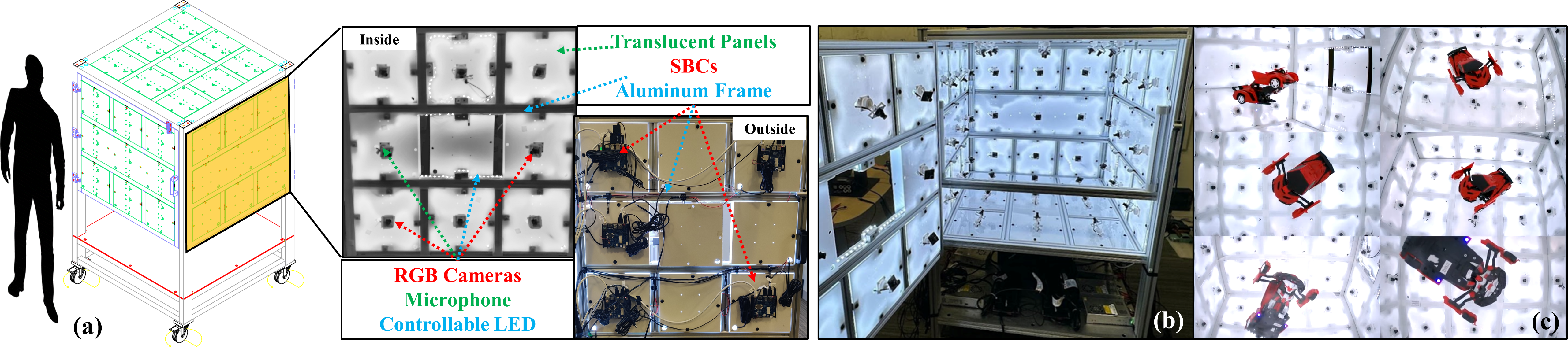
Figure 2: (a) TRICS is a refrigerator-sized aluminum frame that supports a 1m³ capture volume mounted on wheels for mobility. Each side wall of the capture volume is divided into a 3$\times$3 grid with each grid square containing sensors, LEDs, single-board computers (SBCs), and light diffusers. (b) Two walls of the capture volume act as doors for easy access to the capture volume. (c) We can acquire 360^∘ RGB views of dynamic and static objects in this capture volume (6 views shown).

TRICS Software:  While our hardware allows the capture of large-scale rich multimodal data, controlling the sensors and LEDs, synchronizing and managing data, and camera calibration requires specialized software which we have developed. For camera and microphone synchronization, we adopt network-based synchronization [3] with an accuracy of 2–3ms. For camera calibration, during each capture session, we affix transparent curtains with ArUco markers to the walls. Using COLMAP [61, 62], we generate camera poses for the 53 cameras. The camera poses are further refined using Instant-NGP’s [48] dense photometric loss for improved reconstruction quality. Finally, we also built software for efficiently transferring terabytes of data from the control workstation to cloud storage. We will release all of our software for community use.

4 DiVA-360 Dataset

We now describe our multimodal dynamic and static datasets that have been captured using TRICS. While other datasets have focused on in-the-wild capture and a large number of categories [29, 56], our goal is to focus on rich synchronized and multimodal data at high resolution, framerate, spanning long duration, and captured from all 360^∘ volume within the capture space. Our dataset contains 8.6 M image frames of 46 prolonged dynamic scenes over 1360 seconds, 95 static objects across 11 categories, and text descriptions totaling 8632 words.

4.1 Dynamic Dataset

The DiVA-360 dynamic dataset contains synchronized long-duration audio-video of both moving objects and hand interactions. Our goal is to make this dataset useful for learning long-duration dynamic neural fields of appearance and audio – existing methods have been limited to only short durations and lack audio [36, 72]. We captured 21 dynamic objects and 25 hand interactions with objects for a total of 1360 seconds of audio-visual data from TRICS (see Figure 3). Our data also contains masks for foreground-background segmentation and detailed text descriptions of each sequence. To our knowledge, this is the largest-scale multimodal audio-visual dynamic dataset.

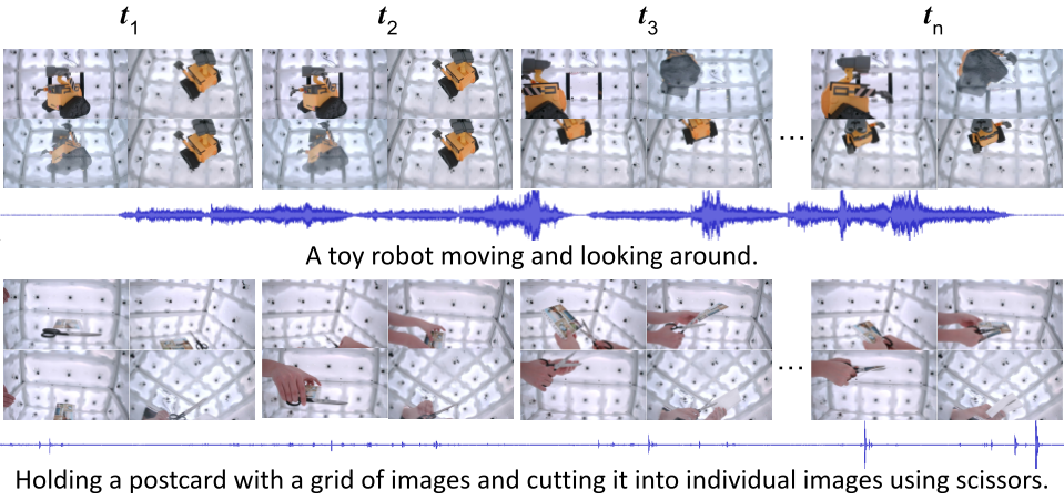
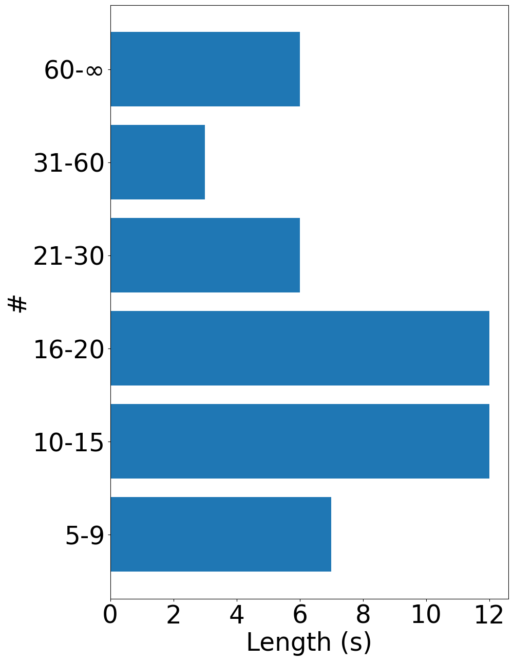
Figure 3: The DiVA-360 dynamic dataset contains multiview images and audio of dynamic objects (top row) and scenes (bottom), including routine human activities, musical instrument play, and objects moving or playing themselves. Our audio component (displaying 1 of 6 channels) contains both loud (e.g., top) and more subtle sounds (e.g., bottom) of objects in motion. On the right, we show the duration distribution of our sequences.

Dynamic Objects:  We selected 21 dynamic objects that move and produce sounds. To be representative of real-world motions, we chose scenes with different types of motion: (1) Slow motion: objects that perform slow, continuous motions, e.g., music box and rotating world globe. (2) Fast motion: objects that move or transform drastically, e.g., remote control cars and dancing toys. (3) Detailed motion: objects that perform precise motions, e.g., a clock. (4) Repetitive motion: objects that repeat the same motion pattern, e.g., Stirling engine and toys that sway left and right. (5) Random motion: objects that perform indeterministic motions, e.g., plasma ball and sand in an hourglass. During capture, all objects are placed on a transparent shelf for 360^∘ view.

Interactions:  In addition to dynamic objects, we also include 25 hand-object interaction scenes representing real-world activities. The interactions included are hand activities commonly observed in everyday life, such as flipping a book, replacing a toy’s batteries, and opening a lock. Most interactions also generate subtle sounds, such as turning a page or opening a soda can. We hope these hand-centric interactions encourage future modeling of complex hand dynamics. Similar to dynamic objects, the objects to be manipulated are placed on a transparent shelf.

Text Descriptions:  Each dynamic scene is accompanied by natural language descriptions at 3 levels of detail. These descriptions are generated entirely by a human annotator without the assistance of any automated tools. As such, we provide a human baseline for tasks that aim to align 3D visual representations with natural language. The coarsest level aims to capture a broad summary of the scene (“putting candy into a mug”), while finer levels increasingly describe appearance (“…the pieces are in pink, green, orange, and black wrappers…”), relative position (“…candy scattered around a black mug…”), number of hands, audio, and temporal progression. Across all 46 dynamic scenes, the average length of the descriptions is 6.1, 18.4, and 38.7 words for the 3 levels of detail, amounting to a total of 2907 words.

Foreground-Background Segmentation:  A major challenge in our dataset is the segmentation of foreground objects from background clutter. Manually segmenting every frame is infeasible due to the quantity and view inconsistency. Therefore, we developed a segmentation method using Instant NGP [48]. As preparation, we manually segment the foreground object in the first frame of one scene and train an I-NGP model on segmented images to refine coarse camera poses extracted from COLMAP[61, 62]. The refined pose is used for all downstream tasks. For each frame, we fit an I-NGP model that optimizes camera poses, lens distortion, and image latent vector. The model’s bounding box is then progressively reduced to remove background clutter. We then render trained I-NGP as binary masks. To further refine the masks, we removed connected components smaller than a threshold. Segmenting with this method is possible because all objects are placed around the center of TRICS. Since the segmentation is generated from I-NGP, the masks are multi-view consistent.

We analyze and compare the our DiVA-360 dynamic dataset with other dynamic datasets and two

	Object			Dynamic Scene
Dataset	#Objects	#Categories		#Scenes	#Frames	Average length (s)
CO3D[56]	19k	50		—	—	—
OmniObject3D[76]	6k	190		—	—	—
Objaverse[18]	818k	21k		3k	$\infty$	—
DyNeRF[36]	—	—		6	37.8k	10
HyperNeRF[54]	—	—		17	13.8k	27
Deep3DMV[40]	—	—		96	3.8M	33
ILFV[8]	—	—		15	270.4k	13
Block-NeRF[66]	—	—		1	12k	100∗
DiVA-360	95	11		46	8.6M	29.6

Table 2: Specifications of our DiVA-360 dataset and other dynamic datasets and large-scale object-centric datasets. $*$ indicates that despite Block-NeRF comprising a 100s-long video, it is made up of numerous transient street scenes, each with restricted view coverage.

large object-centric datasets in Table 2. DyNeRF [36] consists of only 6 short clips of forward-facing scenes. Block-NeRF [66] captures a single long video of a street view from a moving vehicle. This creates fleeting scenes that do not encompass full 360^∘ camera coverage. Though Objaverse offers an expansive repository of animations, it lacks real-world scenes resulting in a domain gap. Our dataset incorporates extensive, prolonged dynamic sequences from 53 different viewpoints, effectively eliminating any blind spots within the dynamic components of the scene. In Section 5, we show how this data can be used to study dynamic neural field models and we provide metrics for comparison. We believe our synchronized audio and video data will spur new research.

4.2 Static Dataset

The DiVA-360 static dataset contains 360^∘ 53-view images of 95 objects spanning 11 categories captured at two orientations, and 30 multi-object scenes captured (5 clean and 25 messy). Our goal is to make this dataset useful for categorical neural field learning for real-world objects. This dataset also contains language descriptions for each object instance at 3 levels of detail. Finally, to support category-level 3D learning, we provide the 6 degrees of freedom (DoF) pose of all object instances. In total, this data contains 11,660 images and 5725 words of text descriptions (see Figure 4).

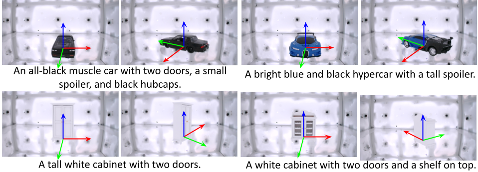
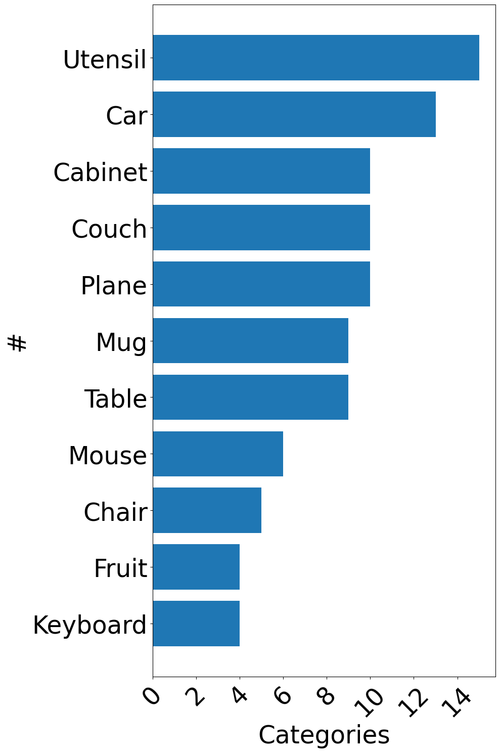
Figure 4: We showcase 4 pairs of captured static objects in a pre-defined canonical pose (left) and random poses (right) for each category. The histogram on the right shows our dataset includes a variety of objects from common shape categories.

Objects:  The static dataset contains categories of objects similar to those found in ShapeNet [10] (e.g., cars, airplanes, cabinets), as well as common objects found in everyday life (e.g., utensils, mugs, keyboards). We also collected 30 multi-object scenes to resemble miniature rooms in both cluttered and cleanly-arranged settings [75]. For single objects, we first capture them in a pre-specified category-level canonical orientation followed by a random orientation. Similarly, for multi-objects, we first capture them in a “clean” state and rearrange the objects to capture increasingly messy states.

Text Descriptions:  As in the dynamic dataset, we provide the natural language descriptions of the objects at 3 levels of detail generated entirely by a human annotator. For these static objects, the coarsest level provides a brief, generic description (“a black car”), while finer levels introduce details in appearance (“an all-black muscle car…”) and aim to differentiate the object within its class (“…with two doors…”). Across all 125 static scenes, the average length of the descriptions is 4.8, 10.9, and 30.2 words for the 3 levels of detail, amounting to a total of 5725 words.

Canonicalization:  We provide category-level canonicalization for each of the static object categories, which provides an equivariant frame of reference that is consistent in position and orientation (3D pose) at the category level [57]. We automatically canonicalize objects using Canonical Fields Network (CaFi-Net) [2]. CaFi-Net uses a Siamese network architecture to extract equivariant field features from the neural field of object instances in arbitrary poses, and estimate a transformation that maps input to a canonical pose. We use CaFi-Net because of its self-supervised nature to estimate the canonical pose of each category.

While the scale of objects and categories in our dataset is smaller compared to CO3D and OmniObject3D, it compensates with rich textual annotations, and each object category is consistently presented in a canonical pose, which facilitates the learning of category-level 3D representations. We hope that our DiVA-360 static dataset will accelerate research in object-centric learning in neural fields. In Section 5, we show how this data can be used to evaluate methods for static neural field reconstruction and provide metrics for 6 DoF pose canonicalization.

5 Benchmarks & Experiments

We show how DiVA-360 can be used to as a benchmark for neural field methods. We propose to standardize metrics for comparisons across methods and provide results of baselines on these metrics. All our experiments use Nvidia GPUs (2080Ti, 3090, 4090, A5000) for training and evaluation.

5.1 DiVA-360 Dynamic

Our goal is to evaluate existing methods for dynamic neural field reconstruction on image reconstruction quality. Specifically, we choose to compare two methods: (1) MixVoxels [72], a state-of-the-art method designed for dynamic radiance field reconstruction, and (2) Per-Frame I-NGP (PF I-NGP) [48], a static NeRF model which we fit to individual frames in all 46 sequences.

Pre-processing:  We downsample the videos to 30 FPS and then segment all frames following Section 4. We select the top 35 out of 53 best cameras for training and hold out 6 cameras for testing.

Metrics:  We use (a) Peak Signal-to-Noise Ratio (PSNR), (b) Structural Similarity Index Measure (SSIM) [59, 70], (c) Learned Perceptual Image Patch Similarity (LPIPS) [85] to measure the rendering quality, and Just Objectionable Difference (JOD) [43] to measure the visual difference between rendered video and ground truth, along with per-frame training/rendering time (s) for 6 testing views.

Baseline	PSNR$\uparrow$	SSIM$\uparrow$	LPIPS$\downarrow$	JOD$\uparrow$	Train (s/f)$\downarrow$	Render (s/f)$\downarrow$
MixVoxels[72]	27.39 $\pm$ 2.35	0.94 $\pm$ 0.02	0.09 $\pm$ 0.03	7.53 $\pm$ 1.09	66.33 $\pm$ 43.19	1.77 $\pm$ 0.52
PF I-NGP[48]	28.13 $\pm$ 3.50	0.95 $\pm$ 0.03	0.08 $\pm$ 0.04	7.61 $\pm$ 0.93	48.85 $\pm$ 4.73	0.67 $\pm$ 0.18

Table 3: We compare the rendering quality and train/render time of MixVoxels and PF I-NGP for dynamic scenes. Not surprisingly, PF I-NGP achieves higher rendering quality as it trains a model for each individual frame, though it lacks temporal coherence. In contrast, MixVoxels exhibits a much more compact form. The time is measured in seconds per frame (s/f).

Results and Analysis:  We quantitatively compare the two baseline methods MixVoxels and PF I-NGP in Table 3. Since PF I-NGP fits each frame individually and has more network capacity, its overall reconstruction performance is better than MixVoxels (see Figure 5 and Figure 6). However, MixVoxels only requires 2.7-4.7 MB storage space per time step, which is six times smaller than PF I-NGP’s 29 MB.

Surprisingly, although MixVoxels is designed for dynamic scenes, its training and inference times are higher than PF I-NGP (with a higher variance). Besides, we also notice that MixVoxel struggles to capture the dynamic components of the scenes, leading to blurry and noisy reconstruction (Figure 6 bottom). In the supplement, we provide more details on the differences between the methods for various scenes. Our primary objective is to establish initial baseline and serve as a resource for future research aimed at enhancing these aspects.

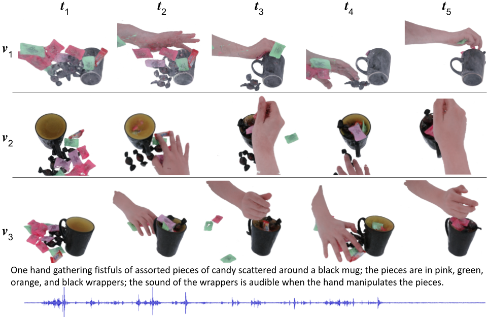
Figure 5: Qualitative results of PF I-NGP on dynamic scene. We show 3 views, 5 timestamps, text descriptions, and 1 audio channel. PF I-NGP has good per-frame quality but lacks temporal consistency.

5.2 DiVA-360 Static

To help build neural field representation for entire categories of objects, our dataset provides canonical-oriented objects, which helps category-level understanding and generalization [65, 37, 49, 73, 58]. We use our object data captured in both canonical pose and random poses to benchmark neural object canonicalization methods [2] to facilitate future research in category-level 3D perception. We also provide a benchmark for rendering quality using I-NGP [48].

Pre-processing:  We segment objects using the Segment Anything Model (SAM) [34] followed by

Categories	CC $\downarrow$	IC $\downarrow$	Categories	CC$\downarrow$	IC $\downarrow$
chair	0.0411	0.0203	keyboard	0.1396	0.0719
table	0.0630	0.0292	car	0.0626	0.0224
cabinet	0.0736	0.0374	couch	0.0604	0.0343
mouse	0.0443	0.0494	plane	0.0538	0.0443
utensil	0.1536	0.1134

Table 4: Object canonicalization benchmark using CaFiNet [2]. The performance is reasonably well for structured shapes such as chairs and tables but it struggles with smaller shape such as utensils.

fitting an I-NGP model (Section 4).

Metrics:  We train I-NGP on 34 best views and validate on 6 held-out views. We use the same PSNR, SSIM [59, 70], LPIPS [85] metrics for evaluation. We provide a benchmark on categorical neural object canonicalization using CaFi-Net [2]. For evaluation, we use the Instance-Level Consistency (IC) and Category-Level Consistency metrics [57].

Results and Analysis:  In Table 5, we notice that some category has much better results than others leaving room for future improvements. Furthermore, segmentation artifacts appear in some scenes with more intricate and detailed geometries, encouraging future work in neural surface reconstruction. The training time for each object instance was 60.51 s (35,000 iterations), and the mean rendering time for  6 validation views was 0.29 s per frame. Table 4 shows the results of canonicalization performance on various categories (we exclude two categories with few instances). CaFi-Net shows good performance on categories with structured 3D shapes (e.g., tables) and sufficient instances.

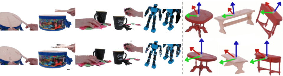
Figure 6: Qualitative comparison of PF I-NGP and MixVoxels and results on CaFiNet[2]. We show rendering from PF I-NGP (top) and MixVoxels (bottom) on the left and show canonicalization results on the right (top: randomly oriented table NeRFs, bottom: canonicalized tables). MixVoxels frequently generates artifacts like floaters or holes, particularly in the most dynamic components such as drumsticks and hands.

Category	PSNR $\uparrow$	SSIM∗ $\uparrow$	LPIPS∗ $\downarrow$	Category	PSNR $\uparrow$	SSIM∗ $\uparrow$	LPIPS∗ $\downarrow$
Chair	32.95$\pm$2.11	98$\pm$0.9	5$\pm$2.3	Keyboard	31.57$\pm$1.58	97$\pm$0.8	7$\pm$1.0
Table	38.11$\pm$1.88	99$\pm$0.3	2$\pm$0.6	Car	34.06$\pm$1.40	98$\pm$0.4	3$\pm$0.5
Cabinet	38.02$\pm$1.65	99$\pm$0.3	3$\pm$0.8	Couch	32.87$\pm$1.51	98$\pm$0.6	4$\pm$0.9
Mug	32.98$\pm$2.12	98$\pm$0.6	4$\pm$0.7	Plane	34.04$\pm$3.30	98$\pm$0.8	4$\pm$2.1
Fruit	34.91$\pm$2.36	99$\pm$0.3	3$\pm$0.8	Utensil	36.45$\pm$3.19	99$\pm$0.4	6$\pm$2.9
Mouse	35.03$\pm$2.40	99$\pm$0.2	3$\pm$0.4	Scenes	27.41$\pm$2.48	95$\pm$2.0	8$\pm$2.7

Table 5: Rendering quality for static object categories and scenes using Instant-NGP [48]. Metrics with (*) are multiplied by 10² to accommodate space. Notice that some categories perform better than others, suggesting future methods that better generalize to a variety of shapes.

6 Conclusion

We have introduced DiVA-360, a real-world 360^∘ dynamic visuo-audio dataset that contains synchronized multimodal visual, auditory, and textual information about table-scale objects and interactive scenes. We propose a new TRICS capture system for rich multimodal data capture. DiVA-360 consists of a dynamic dataset of high-resolution, high-framerate, long (5s to 3 mins), and audio-synchronized videos captured simultaneously from 53 RGB cameras and 6 microphones spanning 360^∘ volume within the capture space. Our static data similarly includes high-resolution 53-view images and category-specific 6 DoF pose alignment for object instances. In addition, both static and dynamic scenes contain detailed text descriptions of the scene or interaction and mask annotations to separate the foreground from the background.

Limitations and Future Work:  Our focus is intentionally on high-quality multimodal data rather than the number of scenes or objects, but large-scale learning is also essential and provided by datasets like [56, 76]. Our metrics and evaluation are limited to images – in future work we will consider metrics for audio and text. TRICS cannot capture scenes larger than table-scale – we plan to expand this to larger volumes and in-the-wild capture in the future.

Societal/Ethical Impact:  Our dataset does not reveal any private information and presents limited means for misuse. However, future extensions of our work could contain private information that can be misused. Furthermore, the multimodal nature of the dataset presents challenges in reducing misuse and leaking of personal data that future research should explore.

Acknowledgments:  This work was supported by NSF grants CAREER #2143576 and CNS #2038897, ONR grant N00014-22-1-259, a gift from Meta Reality Labs, an AWS Cloud Credits award, and NSF CloudBank. Arnab Dey was supported by H2020 COFUND program BoostUrCareer under Marie SklodowskaCurie grant agreement #847581. We thank George Konidaris, Stefanie Tellex, and Rohith Agaram.

Appendix A Author Statement

As the authors of this dataset, we assume full responsibility for all the information provided herein and commit to addressing any potential violations of data rights and other ethical standards promptly. We affirm that the data collection and use are in compliance with all relevant regulations, and the dataset is shared under an MIT license allowing use, redistribution, and citation in line with the license terms.

Appendix B Design of Temporal Interaction Capture System (TRICS)

Aluminum Frame:  To capture table-scale scenes, we chose a refrigerator-sized aluminum frame (Figure 2 (a)) that houses a 1m³ capture volume mounted on wheels for mobility. Each of the 6 side walls of the capture volume is composed of a 3$\times$3 grid with dual polycarbonate panels on each grid square (total of 54 squares). Two of the walls are doors that allow quick access to the capture volume. The height of the system allows an average person to easily reach into the volume for interaction capture. A transparent polycarbonate shelf in the capture volume allows bottom cameras to still see objects to provide a 360^∘ view. A shelf in the bottom houses power supplies, network switches, and a control workstation.

Sensor/Illumination Panels:  For 53 of the 54 grid squares (we leave one out for easy access) on the side walls, we installed translucent polycarbonate panels on the interior consisting of cameras, microphones, and LEDs. Each panel can support up to 3 RGB cameras, 3 microphones, and a fully-programmable RGB light strip with 72 individual LEDs. This panel naturally diffuses the LED lights enabling uniform lighting of the volume. In our current setup, each of the 53 panels has an LED strip and 1 off-the-shelf RGB camera capturing at 1280$\times$720 @ 120 FPS. We install microphones on 6 panels, one on each side wall of the capture cube. Because the LED colors are fully programmable, our capture volume also acts as a light stage [16].

Communication Panels:  The sensor panels collectively generate more than 13.25 GB/s (0.25 GB/s per panel) of uncompressed data – well beyond the bandwidth of common wired communication technologies like USB or ethernet. To enable the capture and storage of such amounts of data, we built our own communication system. Briefly, this system consists of single-board computers (SBCs) that connect to sensors via USB and are responsible for compressing the data before sending it to a control station over gigabit ethernet. With this setup, we are able to simultaneously transmit large amounts of data with low latency.

Control Workstation:  We use a workstation with 52 CPU cores to simultaneously uncompress, store, and transmit all the data. To ensure high throughput, we use a 10 Gigabit ethernet uplink to the SBCs, a PCI solid state drive, and 200 GB RAM for caching.

Panels:  TRICS panels are designed to be modular, to allow for quick customization for different research endeavors. TRICS consists of 42 panels in total across six sides. Each side has six square panels of size (9.75in x 9.75in) and single rectangular middle panel of size (32.25in x 9.75in) that can be changed to consist of three square panels based on research tasks. The panels inside are white translucent panels made of TAP plastics Satinice White Acrylic to encourage light dispersion towards the inside. Outer panels are white and opaque made of TAP plastics KOMATEX foamed PVC Sheets.

The inner panels allow mounting of three different cameras or other accessories. Although the panel currently consists of an RGB camera of size (71.5mm x 71.5mm) mounted at the center, future plans include attaching depth and infrared cameras. All panels are 1/8th inch in thickness.

Mounts:  We utilize custom designed mounts to attach cameras to the panels. We use custom designed ball bearing mounts, that are rotatable to allow for changing the camera orientation.

Lighting:  We use BTF-Lighting WS2812-B individually addressable RGB lighting strips. This allows for highly customized lighting conditions and environment maps. Moreover, using LED strips allows us to add additional lighting quickly.

Each panel has 70 LED’s placed in between the inner panel and outer panel. These LED’s are powered individually and sequentially connected for data. The LED’s are all controlled with six Raspberry Pi 3 Model B+ computers, one for each side. To control the LED’s we used the standard NeoPixel python library. Furthermore, each side allows for individual brightness control.

Cameras:  We used off-the-shelf USB 2.0 cameras that can capture 1280$\times$720 @ 120 FPS. Specifically, we used the ELP-SUSB1080P01-LC1100 from ELP Cameras.

Single Board Computers (SBCs):  We need the single board computers to have enough processing power and USB ports to support upto 3 cameras and 1 microphone each. For this reason and easy market availability, we chose the Odroid N2+ 4 GB which was sufficient for our purpose.

Appendix C Dynamic Dataset Benchmark

Pre-processing:  To do benchmark, we pre-process the raw data captured through TRICS following Section 5. Considering that not every NeRF model supports the camera distortion factor, we undistort the images with OpenCV [6] and crop the images to the same size after undistortion.

Baselines Training:  Per-frame I-NGP sequentially learns a model for each time step. Each I-NGP is initialized from the model of the previous time step. The Per-frame I-NGP allows us to fit the dynamic video efficiently without considering the motion between frames. In addition, the streamable training feature also allows us to optimize the camera pose and lens distortion individually for each frame. We train each I-NGP for 5000 iterations. The average training time for each I-NGP is 48.85 seconds with a standard deviation of 4.73 seconds. The smaller standard deviation is due to the fact that Per-frame I-NGP does not consider motion.

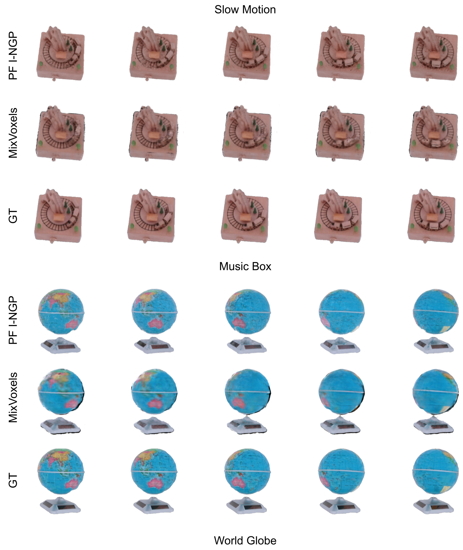
Figure 7: Test view reconstruction from the two baseline models and ground truth of two dynamic objects with slow motion: music box and world globe. Top: Mixvoxels consistently captures the rails on the music box while the reconstruction from I-NGP lacks temporal consistency. Bottom: I-NGP successfully captures the world globe with detail while MixVoxels generates a blurry surface.

Mixvoxels [72] is trained to capture the dynamic video every 150 frames. We train each Mixvoxels for 25000 iterations. We lower the dynamic threshold to capture more dynamic samples for scenes with drastic motion. Unlike per-frame I-NGP, Mixvoxels allows us to learn a dynamic NeRF with motion. In addition, Mixvoxels trained with multiple frames also encourage temporal consistency, which is absent in per-frame I-NGP. We can observe this in the rail of the music box in Figure 7. For each time step, the average training time is 66.33 seconds with a standard deviation of 43.19 seconds. The large standard deviation is due to the fact that Mixvoxels will sample more dynamic points for its dynamic branch when learning a scene with complex motion.

Dynamic Object Results:  Table 6 shows quantitative results of dynamic objects and interactions separately. Both Per-frame I-NGP and MixVoxels perform better when trained with dynamic objects. One reason is that models trained on dynamic objects do not need to handle occlusion caused by the hands. The performance gap of Per-frame I-NGP is 2.73 dB, while the performance gap of MixVoxels is 1.82 dB. The performance gap between dynamic objects and interactions is more obvious with Per-frame I-NGP because it does not utilize temporal information and, therefore, cannot handle occlusion well.

Types	Baseline	PSNR$\uparrow$	SSIM$\uparrow$	LPIPS$\downarrow$	JOD$\uparrow$
Dynamic objects	Per-frame I-NGP[48]	29.62 / 4.42	0.95 / 0.02	0.06 / 0.02	7.53 / 1.28
	MixVoxels[72]	28.40 / 2.75	0.94 / 0.03	0.07 / 0.02	7.44 / 1.54
Interactions	Per-frame I-NGP[48]	26.89 / 1.76	0.94 / 0.03	0.09 / 0.04	7.68 / 0.51
	MixVoxels[72]	26.58 / 1.62	0.93 / 0.02	0.10 / 0.03	7.61 / 0.54

Table 6: Rendering quality (mean/SD) of dynamic objects and interactions respectively using Per-frame I-NGP[48] and MixVoxels.[72]. Although the PSNR of Per-frame I-NGP is much better than MixVoxels in terms of dynamic objects, the PSNR of Per-frame I-NGP is similar to the Mixvoxels for interactions. This indicates that it is hard to capture the occluded scene without utilizing the temporal information.

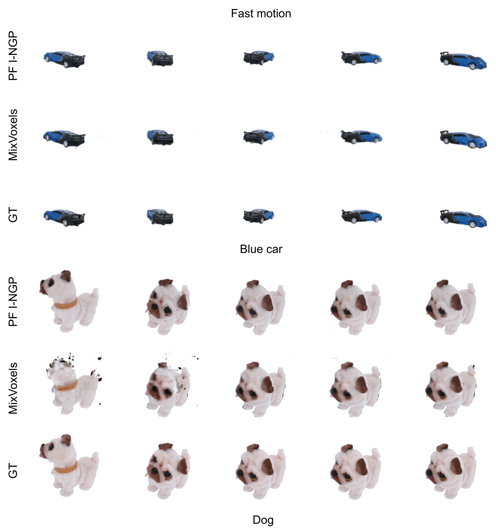
Figure 8: Test view reconstruction and ground truth of two fast motion objects: blue car and dog. Top: both I-NGP and MixVoxels captures the fast continuous motion of the blue car. Botton: MixVoxels fails the capture the dog’s head when it is moving drastically.

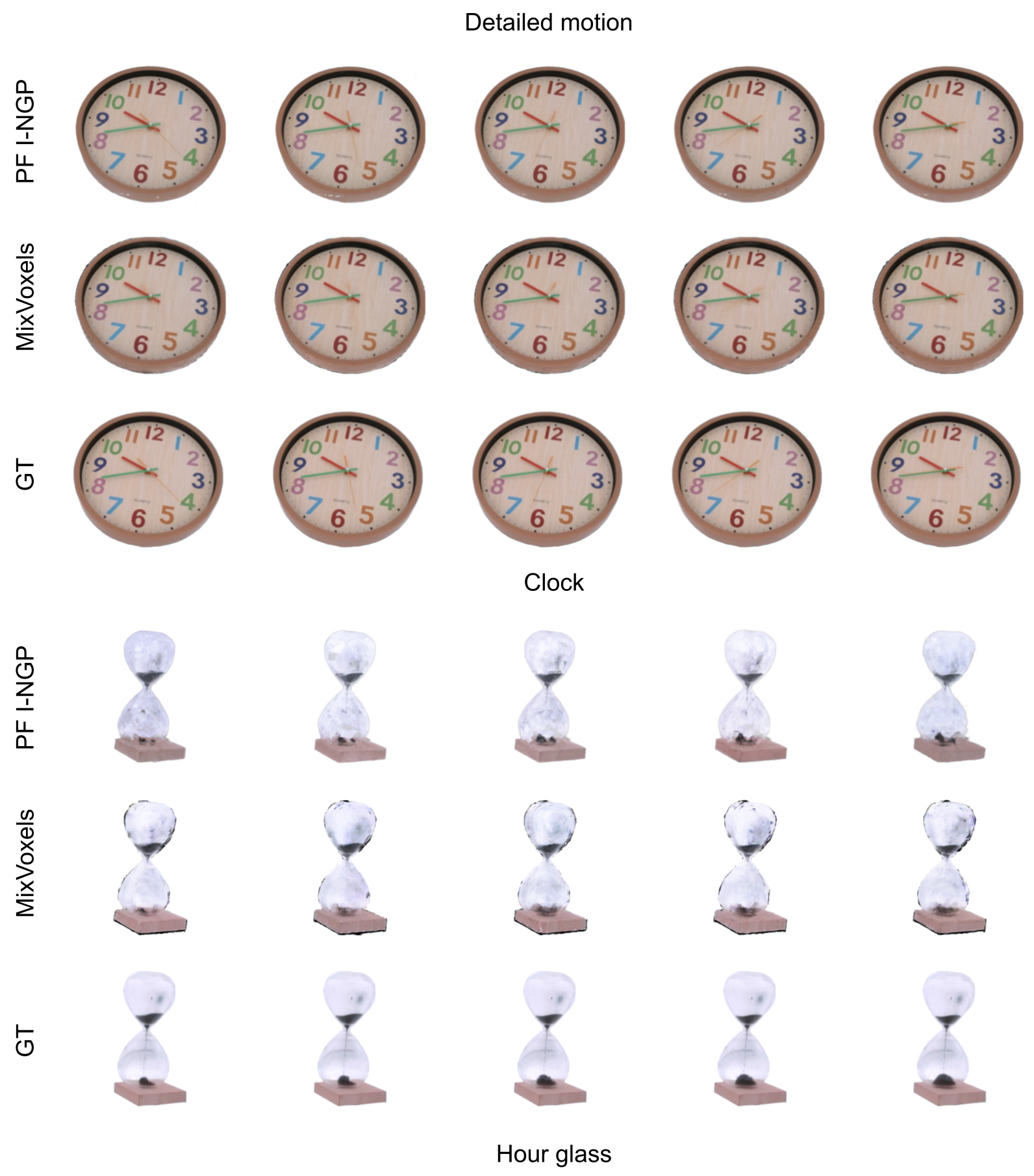
Figure 9: Test view reconstruction and ground truth of two detailed motion objects: clock and hourglass. Top: MixVoxels captures the clock’s body accurately but could not reconstruct the second hand. Bottom: Both I-NGP and MixVoxels cannot reconstruct the hourglass well due to transparency and highly detailed motion.

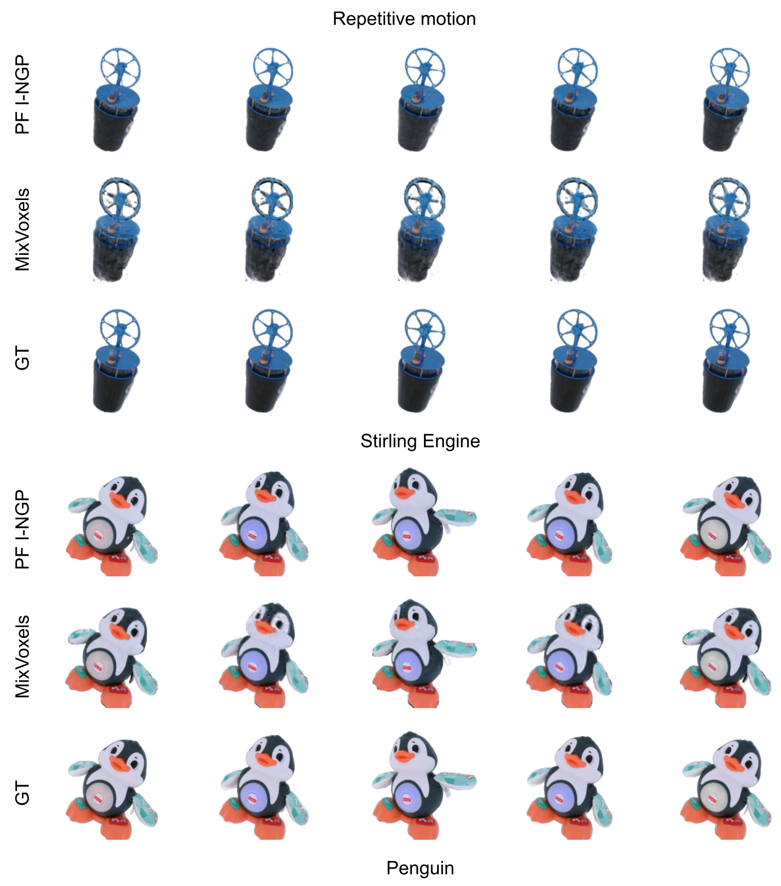
Figure 10: Test view reconstruction and ground truth of two objects with repetitive motions: sterling engine and toy penguin. Top: Both models capture the sterling engine’s motion but I-NGP produces a better reconstruction. Bottom: Both models faithfully capture the penguin’s motion.

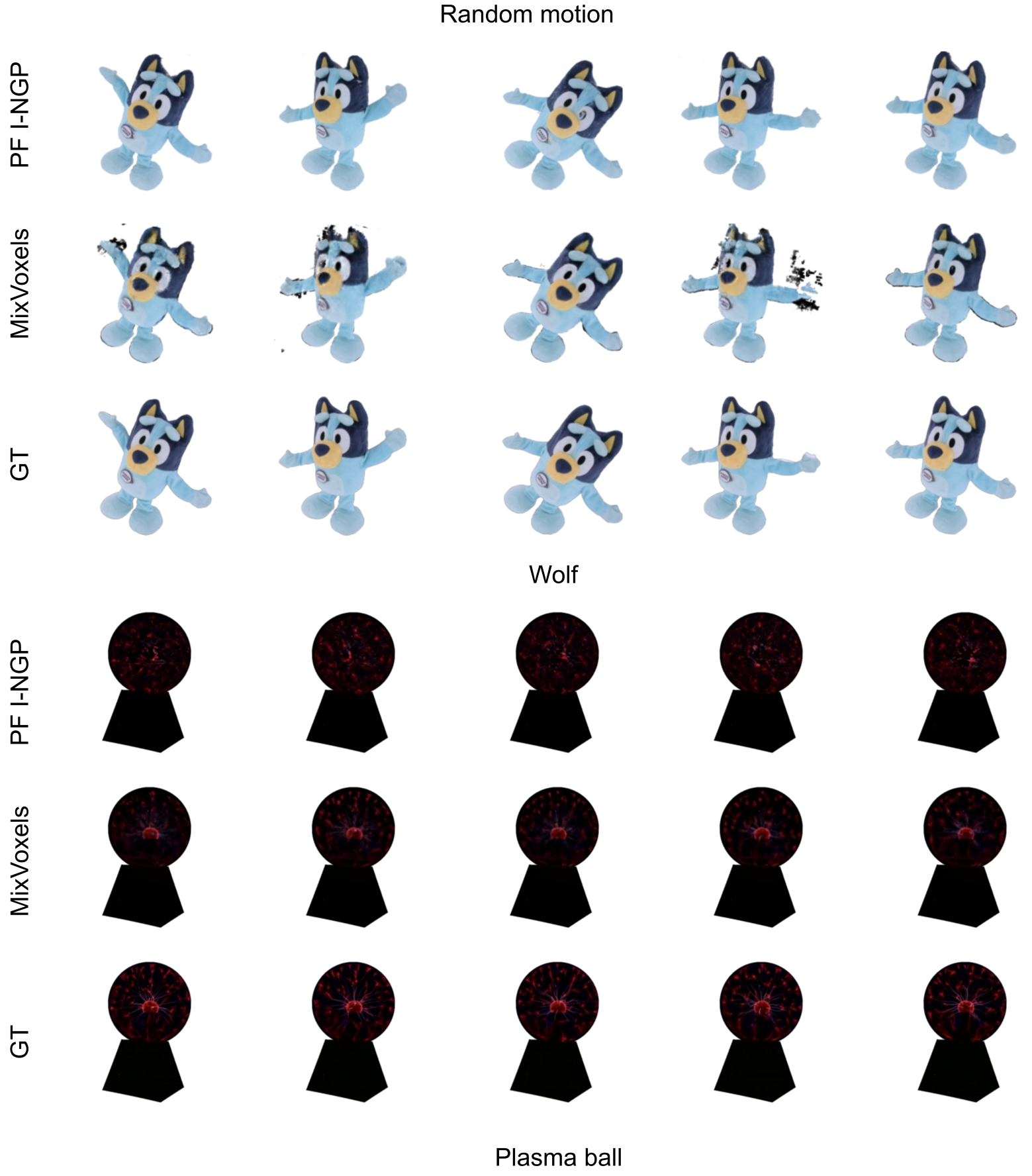
Figure 11: Test view reconstruction and ground truth of two random motion objects: toy wolf and plasma ball. Top: Both models capture the toy’s motion but MixVoxels generates some artifacts and sometimes fails to capture the ear of the wolf. Bottom: MixVoxels captures the currents in the plasma ball surprisingly well while I-NGP completely fails.

Table 7 shows the performance of Per-frame I-NGP and MixVoxels in different motion types. We manually classified the 21 dynamic objects sequence into five overlapping categories: slow, fast, detailed, repetitive, and random (Table 8). Although Per-frame I-NGP does not consider motion, it serves as a baseline for dynamic models by fitting to each frame separately. Both Mixvoxels and Per-frame I-NGP perform the best on detailed motions. However, a huge gap exists between Mixvoxels and I-NGP’s quantitative results, suggesting that Mixvoxels cannot capture detailed motion well but instead only captures the static background, e.g., the second hand of the clock in Figure 9 disappears. Slow and repetitive motions are the two categories that Mixvoxels’ results are the closest to I-NGP’s while the performance gaps are larger in fast and random motions. Furthermore, Mixvoxels’ JOD score surpasses I-NGP, suggesting that Mixvoxels have better temporal consistency. Hence, MixVoxels can successfully capture dynamic information when the motion is continuous and gradual but cannot generalize well to drastic motion. For example, the music box in Figure 7 and the penguin in Figure 10 are clean, while the dog in Figure 8 and the wolf in Figure 11 contain obvious artifacts.

Together with the quantitative results (Table 9), the visualization results suggest that Per-frame I-NGP can successfully capture most of the scene while suffering from temporal inconsistency, while Mixvoxels struggles to generalize to different types of motions and requires hyperparameter tuning to fit scenes with more dramatic motions.

Baseline	Motion	PSNR$\uparrow$	SSIM$\uparrow$	LPIPS$\downarrow$	JOD$\uparrow$
Per-frame I-NGP[48]	Slow	29.76 / 2.18	0.96 / 0.02	0.05 / 0.03	7.13 / 2.57
	Fast	30.05 / 5.14	0.95 / 0.01	0.06 / 0.01	7.60 / 0.60
	Detailed	33.11 / 7.80	0.95 / 0.02	0.07 / 0.03	6.74 / 2.35
	Repetitive	28.76 / 2.16	0.95 / 0.02	0.06 / 0.02	7.75 / 0.71
	Random	31.58 / 8.95	0.95 / 0.01	0.07 / 0.02	6.74 / 2.34
MixVoxels[72]	Slow	29.57 / 2.10	0.96 / 0.02	0.05 / 0.03	7.57 / 2.55
	Fast	28.37 / 2.93	0.94 / 0.03	0.07 / 0.02	7.28 / 1.21
	Detailed	30.12 / 3.78	0.93 / 0.05	0.07 / 0.03	6.88 / 2.64
	Repetitive	28.42 / 2.22	0.95 / 0.03	0.06 / 0.02	7.62 / 1.39
	Random	27.81 / 5.59	0.95 / 0.02	0.08 / 0.03	6.40 / 2.29

Table 7: Rendering quality (mean/SD) of dynamic objects using Per-frame I-NGP[48] and MixVoxels.[72] in terms of different types of motion. Per-frame I-NGP serves as a baseline without considering temporal information. MixVoxels can capture scenes with slow and repetitive motion well, but performs poorly on scenes with drastic motion.

Scene	Slow	Fast	Detailed	Repetitive	Random
blue car	✗	✓	✗	✓	✗
bunny	✗	✓	✗	✓	✗
clock	✓	✗	✓	✗	✗
dog	✗	✓	✗	✗	✓
horse	✓	✗	✗	✓	✗
hourglass	✓	✗	✓	✗	✓
k1 double punch	✗	✓	✗	✓	✗
k1 handstand	✗	✓	✗	✗	✗
k1 push up	✗	✓	✗	✓	✗
music box	✓	✗	✗	✓	✗
penguin	✗	✗	✗	✓	✗
plasma ball	✗	✓	✓	✗	✓
plasma ball clip	✗	✓	✓	✗	✓
red car	✗	✓	✗	✓	✗
stirling	✗	✓	✓	✓	✗
tornado	✗	✓	✗	✓	✗
trex	✗	✓	✗	✗	✗
truck	✗	✓	✗	✗	✗
wall-e	✗	✓	✗	✗	✗
truck	✗	✓	✗	✗	✗
wolf	✗	✗	✗	✓	✓
world globe	✓	✗	✗	✓	✗

Table 8: Motion types of each dynamic object. Objects are split into 5 overlapping categories: slow, fast, detailed, repetitive, and random motion.

Scene	I-NGP/Mixvoxels PSNR$\uparrow$	I-NGP/Mixvoxels SSIM$\uparrow$	I-NGP/Mixvoxels LPIPS$\downarrow$	I-NGP/Mixvoxels JOD$\uparrow$
blue car	29.833/29.411	0.957/0.954	0.047/0.052	7.951/8.094
bunny	26.491/25.791	0.941/0.941	0.085/0.082	7.905/8.011
clock	28.943/28.529	0.935/0.933	0.108/0.101	7.810/9.092
dog	25.463/23.181	0.949/0.931	0.085/0.098	7.754/6.790
horse	31.869/31.576	0.982/0.979	0.023/0.024	8.736/8.903
hourglass	27.244/27.554	0.970/0.977	0.054/0.027	2.572/3.049
k1 double punch	27.422/27.463	0.938/0.937	0.070/0.068	6.733/3.544
k1 handstand	27.631/26.901	0.936/0.931	0.072/0.078	7.233/7.346
k1 push up	27.393/27.295	0.936/0.934	0.072/0.073	6.886/7.421
music box	32.225/32.095	0.980/0.979	0.031/0.037	8.444/8.664
penguin	27.034/26.668	0.95/0.950	0.074/0.068	8.182/8.348
plasma ball	33.422/35.746	0.944/0.939	0.072/0.084	7.368/7.893
plasma ball clip	46.476/NA	0.968/NA	0.049/NA	8.139/NA
red car	30.844/30.456	0.961/0.960	0.046/0.059	8.020/7.972
stirling	29.473/28.633	0.966/0.854	0.045/0.070	7.808/7.501
tornado	28.629/28.745	0.965/0.965	0.045/0.043	6.398/6.940
trex	28.496/27.778	0.948/0.944	0.056/0.076	8.257/7.820
truck	31.033/30.228	0.969/0.965	0.038/0.055	8.418/8.220
wall-e	28.164/27.133	0.934/0.922	0.085/0.116	7.597/7.151
wolf	25.341/24.774	0.940/0.935	0.089/0.094	7.855/7.856
world globe	28.529/28.100	0.953/0.954	0.052/0.057	8.063/8.142

Table 9: Rendering quality of all dynamic objects using per-frame instant-NGP[48] and MixVoxels.[72].

All images are evaluated with black backgrounds.

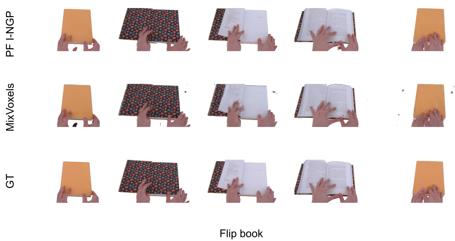
Figure 13: Interaction scene showing the motion of flipping through a book. I-NGP generates some artifacts around the hand and the bottom of the book. MixVoxels generates blurry book pages and hands.

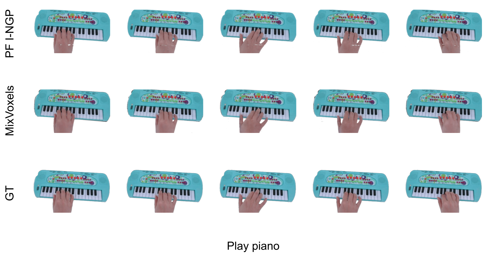
Figure 14: Interaction scene showing a hand playing a toy piano. Both models capture the motion successfully but I-NGP produces some white scratches on the back of the hand.

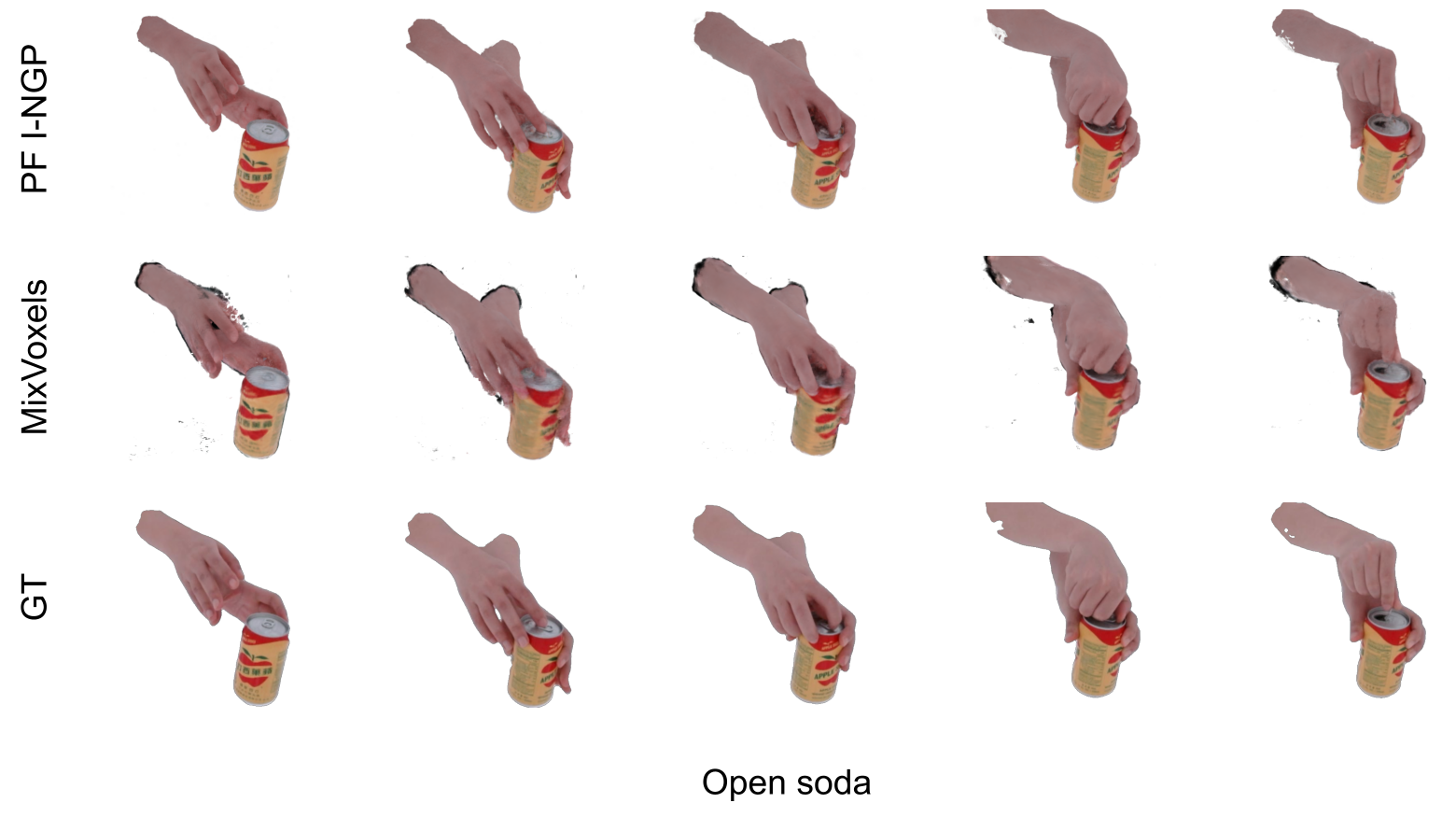
Figure 15: Interaction scene showing the process of opening a can of soda. MixVoxels generate a blurrier can but captures the motion well overall.

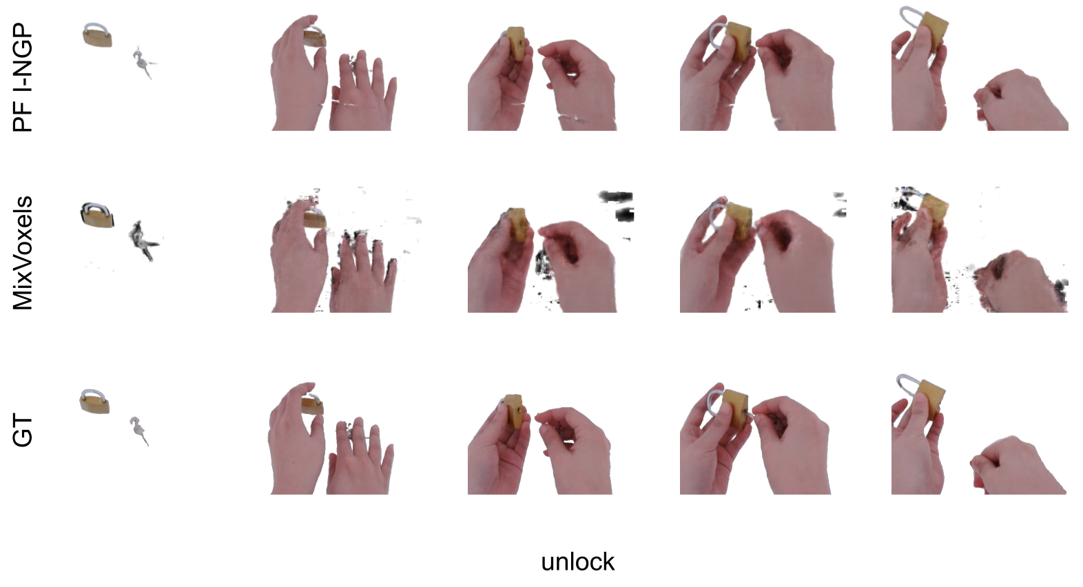
Figure 16: Interaction scene showing the process of unlocking a lock. I-NGP produces white scratches similar to those found in Figure 14.

Interaction Results:  Our interaction scenes require the model to capture a sequence of realistic motions. For example, the battery scene in Figure 12 contains the motion of using a screwdriver to open the toy’s battery cover, putting in the batteries, assembling the cover back, and turning on the toy. Table 10 demonstrates all results of I-NGP and MixVoxels on interaction scenes. Overall, the performances of the two baselines are similar across all interaction scenes. Although both Per-frame I-NGP and MixVoxels can successfully capture hand motions, both miss some details on either the hands or objects. I-NGP fails to reconstruct the bottom part of the book’s cover in Figure 13 while MixVoxels produces book pages with blurrier characters and hands. In Figure 16, MixVoxels can not reconstruct the details of the keyhole and I-NGP generates white scratches on the hand. Similar artifacts are also observed in Figure 14 but are not found in MixVoxels results. Notably, visualization results show black artifacts in Figure 15 and Figure 16 in MixVoxels renderings. This effect is not observable in numerical results because all models are trained and evaluated with black backgrounds. We used white backgrounds for rendering to better visualize the results.

Scene	I-NGP/Mixvoxels	I-NGP/Mixvoxels	I-NGP/Mixvoxels	I-NGP/Mixvoxels
	PSNR$\uparrow$	SSIM$\uparrow$	LPIPS$\downarrow$	JOD$\uparrow$
battery	26.828/26.457	0.931/0.921	0.088/0.109	7.483/7.579
chess	22.945/23.834	0.821/0.867	0.215/0.180	6.756/7.683
drum	24.662/23.836	0.903/0.895	0.136/0.180	7.703/7.000
flip book	26.303/24.357	0.928/0.905	0.12/0.149	7.347/6.271
jenga	29.683/27.543	0.972/0.943	0.046/0.077	8.583/8.470
keyboard mouse	29.635/29.234	0.926/0.926	0.102/0.100	7.808/7.941
kindle	29.556/29.045	0.958/0.951	0.069/0.079	8.237/8.232
maracas	26.083/26.428	0.953/0.950	0.072/0.081	7.659/7.616
pan	27.392/26.604	0.935/0.913	0.094/0.121	7.003/7.052
peel apple	27.270/27.185	0.939/0.941	0.086/0.090	7.843/7.633
piano	26.824/26.045	0.929/0.926	0.104/0.098	7.719/8.484
poker	27.786/27.658	0.958/0.954	0.062/0.068	8.298/8.148
pour salt	25.845/25.658	0.919/0.920	0.104/0.110	7.714/7.480
pour tea	26.071/25.799	0.946/0.941	0.089/0.094	7.447/6.900
put candy	28.189/27.275	0.950/0.942	0.071/0.079	7.906/7.903
put fruit	27.129/26.705	0.935/0.932	0.089/0.095	7.815/7.633
scissor	25.346/24.974	0.944/0.936	0.076/0.086	7.854/7.647
slice apple	26.026/24.964	0.951/0.940	0.106/0.119	7.829/7.403
soda	28.780/28.819	0.964/0.957	0.059/0.076	8.322/7.842
tambourine	27.985/27.191	0.972/0.962	0.044/0.056	7.634/6.947
tea	27.410/27.044	0.956/0.949	0.073/0.097	7.723/6.941
unlock	28.649/29.942	0.971/0.964	0.045/0.071	8.158/7.418
writing 1	24.086/25.226	0.916/0.928	0.158/0.160	6.725/7.761
writing 2	24.345/25.505	0.930/0.934	0.146/0.147	6.490/8.035
xylophone	27.334/27.120	0.950/0.949	0.068/0.066	7.950/8.144

Table 10: Rendering quality of all dynamic interaction scenes using per-frame instant-NGP[48] and MixVoxels.[72].

All images are evaluated with black backgrounds.

Appendix D Static Dataset

Pre-processing:  Our segmentation pipeline for extracting the foreground and background of static objects is divided into two stages: obtaining a coarse mask and refining it. In the first stage, we employ the Segment Anything Model (SAM w/text) [34] to generate a coarse mask by providing each image along with a corresponding object category text description. Subsequently, we apply the I-NGP segmentation in Section 4 to enhance the quality of the coarse masks. However, the segmentation results obtained from this process can exhibit variations with different text prompts and object boundaries may not be very accurate. To address this issue and refine the segmentation, we utilize the SAM (w/bounding box) [34] by inputting the coarse masks generated in the previous stage. This variant of SAM focuses specifically on the local region defined by the bounding box and yields highly accurate segmentation along the object edges. Additionally, we apply the I-NGP segmentation to eliminate any misclassified pixels and achieve a view-consistent segmentation mask. While our aforementioned strategy is effective for single and large objects, we have observed that for scenes with multiple objects or very small objects such as utensils or chairs, the SAM with bounding box input tends to produce erroneous results compared to the SAM with text input. Therefore, for such object categories, we employ the SAM with text input followed by the I-NGP segmentation.

Due to some unavoidable hardware malfunction, scene02_messy1 is missing data for cam49, cam50, and cam52.

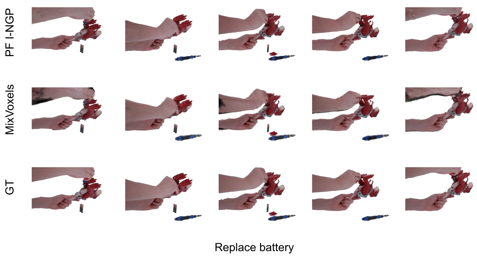
Figure 12: Interaction scene showing the motion of replacing a toy Trex’s battery. The sequence contains a series of realistic motions.

References

- [1] Henrik Aanæs, Rasmus Jensen, George Vogiatzis, Engin Tola, and Anders Dahl. Large-scale data for multiple-view stereopsis. International Journal of Computer Vision, 120, 11 2016.
- [2] Rohith Agaram, Shaurya Dewan, Rahul Sajnani, Adrien Poulenard, Madhava Krishna, and Srinath Sridhar. Canonical fields: Self-supervised learning of pose-canonicalized neural fields. In The IEEE Conference on Computer Vision and Pattern Recognition (CVPR), June 2023.
- [3] Sameer Ansari, Neal Wadhwa, Rahul Garg, and Jiawen Chen. Wireless software synchronization of multiple distributed cameras. In 2019 IEEE International Conference on Computational Photography (ICCP), pages 1–9. IEEE, 2019.
- [4] Jonathan T. Barron, Ben Mildenhall, Matthew Tancik, Peter Hedman, Ricardo Martin-Brualla, and Pratul P. Srinivasan. Mip-nerf: A multiscale representation for anti-aliasing neural radiance fields. ICCV, 2021.
- [5] Jonathan T. Barron, Ben Mildenhall, Dor Verbin, Pratul P. Srinivasan, and Peter Hedman. Mip-nerf 360: Unbounded anti-aliased neural radiance fields. CVPR, 2022.
- [6] G. Bradski. The OpenCV Library. Dr. Dobb’s Journal of Software Tools, 2000.
- [7] Samarth Brahmbhatt, Cusuh Ham, Charles C Kemp, and James Hays. Contactdb: Analyzing and predicting grasp contact via thermal imaging. In Proceedings of the IEEE/CVF conference on computer vision and pattern recognition, pages 8709–8719, 2019.
- [8] Michael Broxton, John Flynn, Ryan Overbeck, Daniel Erickson, Peter Hedman, Matthew DuVall, Jason Dourgarian, Jay Busch, Matt Whalen, and Paul Debevec. Immersive light field video with a layered mesh representation. In ACM Transactions on Graphics (Proc. SIGGRAPH). ACM, 2020.
- [9] Angel Chang, Angela Dai, Thomas Funkhouser, Maciej Halber, Matthias Niessner, Manolis Savva, Shuran Song, Andy Zeng, and Yinda Zhang. Matterport3d: Learning from rgb-d data in indoor environments. International Conference on 3D Vision (3DV), 2017.
- [10] Angel X. Chang, Thomas Funkhouser, Leonidas Guibas, Pat Hanrahan, Qixing Huang, Zimo Li, Silvio Savarese, Manolis Savva, Shuran Song, Hao Su, Jianxiong Xiao, Li Yi, and Fisher Yu. ShapeNet: An Information-Rich 3D Model Repository. Technical Report arXiv:1512.03012 [cs.GR], Stanford University — Princeton University — Toyota Technological Institute at Chicago, 2015.
- [11] Anpei Chen, Zexiang Xu, Andreas Geiger, Jingyi Yu, and Hao Su. Tensorf: Tensorial radiance fields. In European Conference on Computer Vision (ECCV), 2022.
- [12] Changan Chen, Unnat Jain, Carl Schissler, Sebastia Vicenc Amengual Gari, Ziad Al-Halah, Vamsi Krishna Ithapu, Philip Robinson, and Kristen Grauman. Soundspaces: Audio-visual navigation in 3d environments. In ECCV, 2020.
- [13] Zhiqin Chen and Hao Zhang. Learning implicit fields for generative shape modeling. Proceedings of IEEE Conference on Computer Vision and Pattern Recognition (CVPR), 2019.
- [14] Angela Dai, Angel X. Chang, Manolis Savva, Maciej Halber, Thomas Funkhouser, and Matthias Nießner. Scannet: Richly-annotated 3d reconstructions of indoor scenes. In Proc. Computer Vision and Pattern Recognition (CVPR), IEEE, 2017.
- [15] Luca De Luigi, Damiano Bolognini, Federico Domeniconi, Daniele De Gregorio, Matteo Poggi, and Luigi Di Stefano. Scannerf: a scalable benchmark for neural radiance fields. In Winter Conference on Applications of Computer Vision, 2023. WACV.
- [16] Paul Debevec. The light stages and their applications to photoreal digital actors. SIGGRAPH Asia, 2(4):1–6, 2012.
- [17] Paul Debevec, Tim Hawkins, Chris Tchou, Haarm-Pieter Duiker, Westley Sarokin, and Mark Sagar. Acquiring the reflectance field of a human face. In Proceedings of the 27th annual conference on Computer graphics and interactive techniques, pages 145–156, 2000.
- [18] Matt Deitke, Dustin Schwenk, Jordi Salvador, Luca Weihs, Oscar Michel, Eli VanderBilt, Ludwig Schmidt, Kiana Ehsani, Aniruddha Kembhavi, and Ali Farhadi. Objaverse: A universe of annotated 3d objects. arXiv preprint arXiv:2212.08051, 2022.
- [19] Jia Deng, Wei Dong, Richard Socher, Li-Jia Li, Kai Li, and Li Fei-Fei. Imagenet: A large-scale hierarchical image database. In 2009 IEEE conference on computer vision and pattern recognition, pages 248–255. Ieee, 2009.
- [20] Emilien Dupont, Adam Goliński, Milad Alizadeh, Yee Whye Teh, and Arnaud Doucet. Coin: Compression with implicit neural representations. arXiv preprint arXiv:2103.03123, 2021.
- [21] Chen Gao, Ayush Saraf, Johannes Kopf, and Jia-Bin Huang. Dynamic view synthesis from dynamic monocular video. In Proceedings of the IEEE International Conference on Computer Vision, 2021.
- [22] Hang Gao, Ruilong Li, Shubham Tulsiani, Bryan Russell, and Angjoo Kanazawa. Monocular dynamic view synthesis: A reality check. In NeurIPS, 2022.
- [23] Ruohan Gao, Yen-Yu Chang, Shivani Mall, Li Fei-Fei, and Jiajun Wu. Objectfolder: A dataset of objects with implicit visual, auditory, and tactile representations. arXiv preprint arXiv:2109.07991, 2021.
- [24] Ruohan Gao, Zilin Si, Yen-Yu Chang, Samuel Clarke, Jeannette Bohg, Li Fei-Fei, Wenzhen Yuan, and Jiajun Wu. Objectfolder 2.0: A multisensory object dataset for sim2real transfer. In Proceedings of the IEEE/CVF Conference on Computer Vision and Pattern Recognition, pages 10598–10608, 2022.
- [25] Lily Goli, Daniel Rebain, Sara Sabour, Animesh Garg, and Andrea Tagliasacchi. nerf2nerf: Pairwise registration of neural radiance fields. arXiv preprint arXiv:2211.01600, 2022.
- [26] Thibault Groueix, Matthew Fisher, Vladimir G. Kim, Bryan Russell, and Mathieu Aubry. AtlasNet: A Papier-Mâché Approach to Learning 3D Surface Generation. In Proceedings IEEE Conf. on Computer Vision and Pattern Recognition (CVPR), 2018.
- [27] Yudong Guo, Keyu Chen, Sen Liang, Yong-Jin Liu, Hujun Bao, and Juyong Zhang. Ad-nerf: Audio driven neural radiance fields for talking head synthesis. In Proceedings of the IEEE International Conference on Computer Vision (ICCV), 2021.
- [28] Rasmus Jensen, Anders Dahl, George Vogiatzis, Engil Tola, and Henrik Aanæs. Large scale multi-view stereopsis evaluation. In 2014 IEEE Conference on Computer Vision and Pattern Recognition, pages 406–413. IEEE, 2014.
- [29] Yoonwoo Jeong, Seungjoo Shin, Junha Lee, Chris Choy, Anima Anandkumar, Minsu Cho, and Jaesik Park. Perfception: Perception using radiance fields. In Thirty-sixth Conference on Neural Information Processing Systems Datasets and Benchmarks Track, 2022.
- [30] Hanbyul Joo, Hao Liu, Lei Tan, Lin Gui, Bart Nabbe, Iain Matthews, Takeo Kanade, Shohei Nobuhara, and Yaser Sheikh. Panoptic studio: A massively multiview system for social motion capture. In Proceedings of the IEEE International Conference on Computer Vision, pages 3334–3342, 2015.
- [31] Takeo Kanade, Hiroshi Kano, Shigeru Kimura, Atsushi Yoshida, and Kazuo Oda. Development of a video-rate stereo machine. In Proceedings 1995 IEEE/RSJ International Conference on Intelligent Robots and Systems. Human Robot Interaction and Cooperative Robots, volume 3, pages 95–100. IEEE, 1995.
- [32] Takeo Kanade and PJ Narayanan. Virtualized reality: perspectives on 4d digitization of dynamic events. IEEE Computer Graphics and Applications, 27(3):32–40, 2007.
- [33] Justin Kerr, Chung Min Kim, Ken Goldberg, Angjoo Kanazawa, and Matthew Tancik. Lerf: Language embedded radiance fields. arXiv preprint arXiv:2303.09553, 2023.
- [34] Alexander Kirillov, Eric Mintun, Nikhila Ravi, Hanzi Mao, Chloe Rolland, Laura Gustafson, Tete Xiao, Spencer Whitehead, Alexander C. Berg, Wan-Yen Lo, Piotr Dollár, and Ross Girshick. Segment anything. arXiv:2304.02643, 2023.
- [35] Arno Knapitsch, Jaesik Park, Qian-Yi Zhou, and Vladlen Koltun. Tanks and temples: Benchmarking large-scale scene reconstruction. ACM Transactions on Graphics, 36(4), 2017.
- [36] Tianye Li, Mira Slavcheva, Michael Zollhöfer, Simon Green, Christoph Lassner, Changil Kim, Tanner Schmidt, Steven Lovegrove, Michael Goesele, and Zhaoyang Lv. Neural 3d video synthesis. CoRR, abs/2103.02597, 2021.
- [37] Xiaolong Li, He Wang, Li Yi, Leonidas Guibas, A Lynn Abbott, and Shuran Song. Category-level articulated object pose estimation. Proceedings of the IEEE Conference on Computer Vision and Pattern Recognition, 2020.
- [38] Zhaoshuo Li, Thomas Müller, Alex Evans, Russell H Taylor, Mathias Unberath, Ming-Yu Liu, and Chen-Hsuan Lin. Neuralangelo: High-fidelity neural surface reconstruction. In IEEE Conference on Computer Vision and Pattern Recognition (CVPR), 2023.
- [39] Zhengqi Li, Simon Niklaus, Noah Snavely, and Oliver Wang. Neural scene flow fields for space-time view synthesis of dynamic scenes. In Proceedings of the IEEE/CVF Conference on Computer Vision and Pattern Recognition (CVPR), 2021.
- [40] Kai-En Lin, Lei Xiao, Feng Liu, Guowei Yang, and Ravi Ramamoorthi. Deep 3d mask volume for view synthesis of dynamic scenes. In ICCV, 2021.
- [41] Stephen Lombardi, Tomas Simon, Jason Saragih, Gabriel Schwartz, Andreas Lehrmann, and Yaser Sheikh. Neural volumes: Learning dynamic renderable volumes from images. ACM Trans. Graph., 38(4):65:1–65:14, July 2019.
- [42] Andrew Luo, Yilun Du, Michael Tarr, Josh Tenenbaum, Antonio Torralba, and Chuang Gan. Learning neural acoustic fields. Advances in Neural Information Processing Systems, 35:3165–3177, 2022.
- [43] Rafał K Mantiuk, Gyorgy Denes, Alexandre Chapiro, Anton Kaplanyan, Gizem Rufo, Romain Bachy, Trisha Lian, and Anjul Patney. Fovvideovdp: A visible difference predictor for wide field-of-view video. ACM Transactions on Graphics (TOG), 40(4):1–19, 2021.
- [44] Lars Mescheder, Michael Oechsle, Michael Niemeyer, Sebastian Nowozin, and Andreas Geiger. Occupancy networks: Learning 3d reconstruction in function space. In Proceedings of the IEEE/CVF Conference on Computer Vision and Pattern Recognition (CVPR), 2019.
- [45] Lars Mescheder, Michael Oechsle, Michael Niemeyer, Sebastian Nowozin, and Andreas Geiger. Occupancy networks: Learning 3d reconstruction in function space. In Proceedings IEEE Conf. on Computer Vision and Pattern Recognition (CVPR), 2019.
- [46] Ben Mildenhall, Pratul P. Srinivasan, Rodrigo Ortiz-Cayon, Nima Khademi Kalantari, Ravi Ramamoorthi, Ren Ng, and Abhishek Kar. Local light field fusion: Practical view synthesis with prescriptive sampling guidelines. ACM Transactions on Graphics (TOG), 2019.
- [47] Ben Mildenhall, Pratul P. Srinivasan, Matthew Tancik, Jonathan T. Barron, Ravi Ramamoorthi, and Ren Ng. Nerf: Representing scenes as neural radiance fields for view synthesis. In ECCV, 2020.
- [48] Thomas Müller, Alex Evans, Christoph Schied, and Alexander Keller. Instant neural graphics primitives with a multiresolution hash encoding. ACM Trans. Graph., 41(4):102:1–102:15, July 2022.
- [49] David Novotny, Nikhila Ravi, Benjamin Graham, Natalia Neverova, and Andrea Vedaldi. C3dpo: Canonical 3d pose networks for non-rigid structure from motion. In Proceedings of the IEEE International Conference on Computer Vision, 2019.
- [50] Michael Oechsle, Songyou Peng, and Andreas Geiger. Unisurf: Unifying neural implicit surfaces and radiance fields for multi-view reconstruction. In Proceedings of the IEEE/CVF International Conference on Computer Vision, pages 5589–5599, 2021.
- [51] Jeong Joon Park, Peter Florence, Julian Straub, Richard Newcombe, and Steven Lovegrove. Deepsdf: Learning continuous signed distance functions for shape representation. In The IEEE Conference on Computer Vision and Pattern Recognition (CVPR), June 2019.
- [52] Jeong Joon Park, Peter Florence, Julian Straub, Richard Newcombe, and Steven Lovegrove. Deepsdf: Learning continuous signed distance functions for shape representation. In Proceedings of the IEEE/CVF Conference on Computer Vision and Pattern Recognition (CVPR), 2019.
- [53] Keunhong Park, Utkarsh Sinha, Jonathan T. Barron, Sofien Bouaziz, Dan B Goldman, Steven M. Seitz, and Ricardo Martin-Brualla. Nerfies: Deformable neural radiance fields. ICCV, 2021.
- [54] Keunhong Park, Utkarsh Sinha, Peter Hedman, Jonathan T. Barron, Sofien Bouaziz, Dan B Goldman, Ricardo Martin-Brualla, and Steven M. Seitz. Hypernerf: A higher-dimensional representation for topologically varying neural radiance fields. ACM Trans. Graph., 40(6), dec 2021.
- [55] Albert Pumarola, Enric Corona, Gerard Pons-Moll, and Francesc Moreno-Noguer. D-nerf: Neural radiance fields for dynamic scenes. arXiv preprint arXiv:2011.13961, 2020.
- [56] Jeremy Reizenstein, Roman Shapovalov, Philipp Henzler, Luca Sbordone, Patrick Labatut, and David Novotny. Common objects in 3d: Large-scale learning and evaluation of real-life 3d category reconstruction. In International Conference on Computer Vision, 2021.
- [57] Rahul Sajnani, Adrien Poulenard, Jivitesh Jain, Radhika Dua, Leonidas J. Guibas, and Srinath Sridhar. Condor: Self-supervised canonicalization of 3d pose for partial shapes. In The IEEE Conference on Computer Vision and Pattern Recognition (CVPR), June 2022.
- [58] Rahul Sajnani, AadilMehdi Sanchawala, Krishna Murthy Jatavallabhula, Srinath Sridhar, and K. Madhava Krishna. Draco: Weakly supervised dense reconstruction and canonicalization of objects, 2020.
- [59] Umme Sara, Morium Akter, and Mohammad Shorif Uddin. Image quality assessment through fsim, ssim, mse and psnr—a comparative study. Journal of Computer and Communications, 7(3):8–18, 2019.
- [60] Sara Fridovich-Keil and Alex Yu, Matthew Tancik, Qinhong Chen, Benjamin Recht, and Angjoo Kanazawa. Plenoxels: Radiance fields without neural networks. In CVPR, 2022.
- [61] Johannes Lutz Schönberger and Jan-Michael Frahm. Structure-from-motion revisited. In Conference on Computer Vision and Pattern Recognition (CVPR), 2016.
- [62] Johannes Lutz Schönberger, Enliang Zheng, Marc Pollefeys, and Jan-Michael Frahm. Pixelwise view selection for unstructured multi-view stereo. In European Conference on Computer Vision (ECCV), 2016.
- [63] Uriel Singer, Shelly Sheynin, Adam Polyak, Oron Ashual, Iurii Makarov, Filippos Kokkinos, Naman Goyal, Andrea Vedaldi, Devi Parikh, Justin Johnson, and Yaniv Taigman. Text-to-4d dynamic scene generation. arXiv:2301.11280, 2023.
- [64] Vincent Sitzmann, Michael Zollhoefer, and Gordon Wetzstein. Scene representation networks: Continuous 3d-structure-aware neural scene representations. In H. Wallach, H. Larochelle, A. Beygelzimer, F. d'Alché-Buc, E. Fox, and R. Garnett, editors, Advances in Neural Information Processing Systems, volume 32. Curran Associates, Inc., 2019.
- [65] Srinath Sridhar, Davis Rempe, Julien Valentin, Sofien Bouaziz, and Leonidas J. Guibas. Multiview aggregation for learning category-specific shape reconstruction. In Advances in Neural Information Processing Systems (NeurIPS), 2019.
- [66] Matthew Tancik, Vincent Casser, Xinchen Yan, Sabeek Pradhan, Ben Mildenhall, Pratul Srinivasan, Jonathan T. Barron, and Henrik Kretzschmar. Block-NeRF: Scalable large scene neural view synthesis. arXiv, 2022.
- [67] Maxim Tatarchenko*, Stephan R. Richter*, René Ranftl, Zhuwen Li, Vladlen Koltun, and Thomas Brox. What do single-view 3d reconstruction networks learn? CVPR, 2019.
- [68] Ayush Tewari, Justus Thies, Ben Mildenhall, Pratul Srinivasan, Edgar Tretschk, Wang Yifan, Christoph Lassner, Vincent Sitzmann, Ricardo Martin-Brualla, Stephen Lombardi, et al. Advances in neural rendering. In Computer Graphics Forum, 2022.
- [69] Christian Theobalt, Marcus A Magnor, Pascal Schüler, and Hans-Peter Seidel. Combining 2d feature tracking and volume reconstruction for online video-based human motion capture. International Journal of Image and Graphics, 4(04):563–583, 2004.
- [70] Paul Upchurch, Noah Snavely, and Kavita Bala. From a to z: Supervised transfer of style and content using deep neural network generators. CoRR, abs/1603.02003, 2016.
- [71] Kashi Venkatesh Vishwanath, Amin Vahdat, Ken Yocum, and Diwaker Gupta. Modelnet: Towards a datacenter emulation environment. In Henning Schulzrinne, Karl Aberer, and Anwitaman Datta, editors, Peer-to-Peer Computing, pages 81–82. IEEE, 2009.
- [72] Feng Wang, Sinan Tan, Xinghang Li, Zeyue Tian, and Huaping Liu. Mixed neural voxels for fast multi-view video synthesis. arXiv preprint arXiv:2212.00190, 2022.
- [73] He Wang, Srinath Sridhar, Jingwei Huang, Julien Valentin, Shuran Song, and Leonidas J. Guibas. Normalized object coordinate space for category-level 6d object pose and size estimation. In The IEEE Conference on Computer Vision and Pattern Recognition (CVPR), June 2019.
- [74] Yiming Wang, Qin Han, Marc Habermann, Kostas Daniilidis, Christian Theobalt, and Lingjie Liu. Neus2: Fast learning of neural implicit surfaces for multi-view reconstruction, 2022.
- [75] Qiuhong Anna Wei, Sijie Ding, Jeong Joon Park, Rahul Sajnani, Adrien Poulenard, Srinath Sridhar, and Leonidas Guibas. Lego-net: Learning regular rearrangements of objects in rooms. In Proceedings of the IEEE/CVF Conference on Computer Vision and Pattern Recognition, pages 19037–19047, 2023.
- [76] Tong Wu, Jiarui Zhang, Xiao Fu, Yuxin Wang, Jiawei Ren, Liang Pan, Wayne Wu, Lei Yang, Jiaqi Wang, Chen Qian, Dahua Lin, and Ziwei Liu. Omniobject3d: Large-vocabulary 3d object dataset for realistic perception, reconstruction and generation. IEEE/CVF Conference on Computer Vision and Pattern Recognition (CVPR), 2023.
- [77] Zhirong Wu, Shuran Song, Aditya Khosla, Linguang Zhang, Xiaoou Tang, and Jianxiong Xiao. 3d shapenets: A deep representation for volumetric shape modeling. In IEEE Conference on Computer Vision and Pattern Recognition (CVPR), June 2015.
- [78] Wenqi Xian, Jia-Bin Huang, Johannes Kopf, and Changil Kim. Space-time neural irradiance fields for free-viewpoint video. In Proceedings of the IEEE/CVF Conference on Computer Vision and Pattern Recognition (CVPR), pages 9421–9431, 2021.
- [79] Yiheng Xie, Towaki Takikawa, Shunsuke Saito, Or Litany, Shiqin Yan, Numair Khan, Federico Tombari, James Tompkin, Vincent Sitzmann, and Srinath Sridhar. Neural fields in visual computing and beyond. Computer Graphics Forum, 2022.
- [80] Guandao Yang, Serge Belongie, Bharath Hariharan, and Vladlen Koltun. Geometry processing with neural fields. Advances in Neural Information Processing Systems, 34:22483–22497, 2021.
- [81] Yao Yao, Zixin Luo, Shiwei Li, Jingyang Zhang, Yufan Ren, Lei Zhou, Tian Fang, and Long Quan. Blendedmvs: A large-scale dataset for generalized multi-view stereo networks. Computer Vision and Pattern Recognition (CVPR), 2020.
- [82] Lior Yariv, Jiatao Gu, Yoni Kasten, and Yaron Lipman. Volume rendering of neural implicit surfaces. In Thirty-Fifth Conference on Neural Information Processing Systems, 2021.
- [83] Jae Shin Yoon, Kihwan Kim, Orazio Gallo, Hyun Soo Park, and Jan Kautz. Novel view synthesis of dynamic scenes with globally coherent depths from a monocular camera. In Proceedings of the IEEE/CVF Conference on Computer Vision and Pattern Recognition, pages 5336–5345, 2020.
- [84] Zhixuan Yu, Jae Shin Yoon, In Kyu Lee, Prashanth Venkatesh, Jaesik Park, Jihun Yu, and Hyun Soo Park. Humbi: A large multiview dataset of human body expressions. In Proceedings of the IEEE/CVF Conference on Computer Vision and Pattern Recognition, pages 2990–3000, 2020.
- [85] Richard Zhang, Phillip Isola, Alexei A Efros, Eli Shechtman, and Oliver Wang. The unreasonable effectiveness of deep features as a perceptual metric. In CVPR, 2018.
- [86] Christian Zimmermann, Duygu Ceylan, Jimei Yang, Bryan Russell, Max Argus, and Thomas Brox. Freihand: A dataset for markerless capture of hand pose and shape from single rgb images. In Proceedings of the IEEE/CVF International Conference on Computer Vision, pages 813–822, 2019.