Conformal PID Control for Time Series Prediction

Abstract

We study the problem of uncertainty quantification for time series prediction, with the goal of providing easy-to-use algorithms with formal guarantees. The algorithms we present build upon ideas from conformal prediction and control theory, are able to prospectively model conformal scores in an online setting, and adapt to the presence of systematic errors due to seasonality, trends, and general distribution shifts. Our theory both simplifies and strengthens existing analyses in online conformal prediction. Experiments on 4-week-ahead forecasting of statewide COVID-19 death counts in the U.S. show an improvement in coverage over the ensemble forecaster used in official CDC communications. We also run experiments on predicting electricity demand, market returns, and temperature using autoregressive, Theta, Prophet, and Transformer models. We provide an extendable codebase for testing our methods and for the integration of new algorithms, data sets, and forecasting rules.

1 Introduction

Machine learning models run in production systems regularly encounter data distributions that change over time. This can be due to factors such as seasonality and time-of-day, continual updating and re-training of upstream machine learning models, changing user behaviors, and so on. These distribution shifts can degrade a model’s predictive performance. They also invalidate standard techniques for uncertainty quantification, such as conformal prediction [VGS99, VGS05].

To address the problem of shifting distributions, we can consider the task of prediction in an adversarial online setting, as in [GC21]. In this setting, we observe a (potentially) adversarial time series of deterministic covariates $x_{t}\in\mathcal{X}$ and responses $y_{t}\in\mathcal{Y}$, for $t\in\mathbb{N}=\{1,2,3,\dots\}$. As in standard conformal prediction, we are free to define any conformal score function $s_{t}:\mathcal{X}\times\mathcal{Y}\to\mathbb{R}$, which we can view as measuring the accuracy of our forecast at time $t$. We will assume with a loss of generality that $s_{t}$ is negatively oriented (lower values mean greater forecast accuracy). For example, we may use the absolute error $s_{t}(x,y)=|y-f_{t}(x)|$, where $f_{t}$ is a forecaster trained on data up to but not including data at time $t$.

The challenge in the sequential setting is as follows. We seek to invert the score function to construct a conformal prediction set,

$$\mathcal{C}_{t}=\{y\in\mathcal{Y}:s_{t}(x_{t},y)\leq q_{t}\},$$ (1)

where $q_{t}$ is an estimated $1-\alpha$ quantile for the score $s_{t}(x_{t},y_{t})$ at time $t$. In standard conformal prediction, we would take $q_{t}$ to be a level $1-\alpha$ sample quantile (up to a finite-sample correction) of $s_{t}(x_{i},y_{i})$, $i<t$; if the data sequence $(x_{i},y_{i})$, $i\in\mathbb{N}$ were i.i.d. or exchangeable, then this would yield $1-\alpha$ coverage [VGS05] at each time $t$. However, in the sequential setting, which does not assume exchangeability (or any probabilistic model for the data for that matter), choosing $q_{t}$ in (1) to yield coverage is a formidable task. In fact, if we are not willing to make any assumptions about the data sequence, then achieving coverage at time $t$ would require the user to construct prediction intervals of infinite sizes.

Therefore, our goal is to achieve long-run coverage in time. That is, letting $\mathrm{err}_{t}=\mathbbm{1}\left\{y_{t}\notin\mathcal{C}_{t}\right\}$, we would like to achieve, for large integers $T$,

$$\frac{1}{T}\sum_{t=1}^{T}\mathrm{err}_{t}=\alpha+o(1)$$ (2)

under few or no assumptions, where $o(1)$ denotes a quantity that tends to zero as $T\to\infty$. We note that (2) is not probabilistic at all, and every theoretical statement we will make in this paper holds deterministically. Furthermore, going beyond (2), we also seek to design flexible strategies to produce the sharpest prediction sets possible, which not only adapt to, but also anticipate distribution shifts.

We call our proposed solution conformal PID control. It treats the system for producing prediction sets as a proportional-integral-derivative (PID) controller. In the language of control, the prediction sets take a process variable, $q_{t}$, and then produce an output, $\mathrm{err}_{t}$. We seek to anchor $\mathrm{err}_{t}$ to a set point, $\alpha$. To do so, we apply corrections to $q_{t}$ based on the error of the output, $g_{t}=\mathrm{err}_{t}-\alpha$. By reframing the problem in this language, we are able to build algorithms that have more stable coverage while also prospectively adapting to changes in the score sequence, much in the same style as a control system. See the diagram in Figure 1.

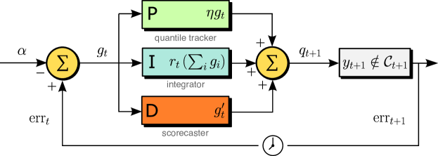
Figure 1: Conformal PID Control, expressed as a block diagram.

1.1 Peek at results: methods

Three design principles underlie our methods:

1. Quantile tracking (P control). Running online gradient descent on the quantile loss (summed over all past scores) gives rise to a method that we call quantile tracking, which achieves long-run coverage (2) under no assumptions except boundedness of the scores. This bound can be unknown. Unlike adaptive conformal inference (ACI) [GC21], quantile tracking does not return infinite sets after a sequence of miscoverage events. This can be seen as equivalent to proportional (P) control.

2. Error integration (I control). By incorporating the running sum $\sum_{i=1}^{t}(\mathrm{err}_{i}-\alpha)$ of the coverage errors into the online quantile updates, we can further stabilize the coverage. This error integration scheme achieves long-run coverage (2) under no assumptions whatsoever on the scores (they can be unbounded). This can be seen as equivalent to integral (I) control.

3. Scorecasting (D control). To account for systematic trends in the scores—this may be due to aspects of the data distribution, fixed or changing, which are not captured by the initial forecaster—we train a second model, namely, a scorecaster, to predict the quantile of the next score. While quantile tracking and error integration are merely reactive, scorecasting is forward-looking. It can potentially residualize out systematic trends in the errors and lead to practical advantages in terms of coverage and efficiency (set sizes). This can be seen as equivalent to derivative (D) control. Traditional control theory would suggest using a linear approximation $g^{\prime}_{t}=g_{t}-g_{t-1}$, but in our problem, we will typically choose more advanced scorecasting algorithms that go well beyond simple difference schemes.

These three modules combine to make our final iteration, the conformal PID controller:

$$q_{t+1}=\underbrace{\vphantom{\Bigg{(}\sum_{i=1}^{t}}\eta g_{t}}_{\text{P}}+\,\underbrace{r_{t}\Bigg{(}\sum_{i=1}^{t}g_{t}\Bigg{)}}_{\text{I}}\,+\underbrace{\vphantom{\Bigg{(}\sum_{i=1}^{t}}g^{\prime}_{t}}_{\text{D}}.$$ (3)

In traditional PID control, one would take $r_{t}(x)$ to be a linear function of $x$. Here, we allow for nonlinearity and take $r_{t}$ to be a saturation function obeying

$$x\geq c\cdot h(t)\implies r_{t}(x)\geq b,\;\;\;\text{and}\;\;\;x\leq-c\cdot h(t)\implies r_{t}(x)\leq-b,$$ (4)

for constants $b,c>0$, and a sublinear, nonnegative, nondecreasing function $h$—we call a function $h$ satisfying these conditions admissible. An example is the tangent integrator $r_{t}(x)=K_{\text{I}}\tan(x\log(t)/(tC_{\text{sat}}))$, where we set $\tan(x)=\mathrm{sign}(x)\cdot\infty$ for $x\notin[-\pi/2,\pi/2]$, and $C_{\text{sat}},K_{\text{I}}>0$ are constants. The choice of integrator $r_{t}$ is a design decision for the user, as is the choice of scorecaster $g^{\prime}_{t}$.

We find it convenient to reparametrize (3), to produce a sequence of quantile estimates $q_{t}$, $t\in\mathbb{N}$ used in the prediction sets (1), as follows:

$$\text{let $\hat{q}_{t+1}$ be any function of the past: $x_{i},y_{i},q_{i}$, for $i\leq t$},$$ (5)

$$\text{then update }q_{t+1}=\hat{q}_{t+1}+r_{t}\Bigg{(}\sum_{i=1}^{t}(\mathrm{err}_{i}-\alpha)\Bigg{)}.$$

Taking $\hat{q}_{t+1}=\eta g_{t}+g^{\prime}_{t}$ recovers (3), but we find it generally useful to instead consider the formulation in (5), which will be our main focus in the exposition henceforth. Now we view $\hat{q}_{t+1}$ as the scorecaster, which directly predicts $q_{t+1}$ using past data. A main result of this paper, whose proof is given in Section 2, is that the conformal PID controller (5) yields long-run coverage for any choice of integrator $r_{t}$ that satisfies the appropriate saturation condition, and any scorecaster $\hat{q}_{t+1}$.

Theorem 1.

Let $\{\hat{q}_{t}\}_{t\in\mathbb{N}}$ be any sequence of numbers in $[-b/2,b/2]$ and let $\{s_{t}\}_{t\in\mathbb{N}}$ be any sequence of score functions with outputs in $[-b/2,b/2]$. Here $b>0$, and may be infinite. Assume that $r_{t}$ satisfies (4), for an admissible function $h$. Then the iterations in (5) achieve long-run coverage (2).

To emphasize, this result holds deterministically, with no probabilistic model on the data $(x_{t},y_{t})$, $t\in\mathbb{N}$. (Thus in the case that the sequence is random, the result holds for all realizations of the random variables.) As we will soon see, this theorem can be seen as a generalization of existing results in the online conformal literature.

1.2 Peek at results: experiments

COVID-19 death forecasting.

To demonstrate conformal PID in practice, we consider 4-week-ahead forecasting of COVID-19 deaths in California, from late 2020 through late 2022. The base forecaster $f_{t}$ that we use is the ensemble model from the COVID-19 Forecast Hub, which is the model used for official CDC communications on COVID-19 forecasting [CHW⁺22, RBB⁺23]. In this forecasting problem, at each time $t$ we actually seek to predict the observed death count $y_{t+4}$ at time $t+4$.

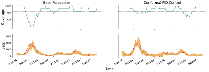
Figure 2: Results for 4-week ahead COVID-19 death forecasting in California. The left column shows the COVID-19 Forecast Hub ensemble model, and the right column shows conformal PID control using the tan integrator, and a scorecaster given by $\ell_{1}$-penalized quantile regression on all past forecasts, cases, and deaths from all 50 states. The top row plots coverage, averaged over a trailing window of 10 weeks. The nominal coverage level is $1-\alpha=0.8$ and marked by a gray dotted line. The bottom row plots the prediction sets in gold along with the ground-truth times series (death counts). Miscoverage events are indicated by red dots. Summary statistics such as the coverage and average set size are available in Table 2.

Figure 2 shows the central 80% prediction sets from the Forecast Hub ensemble model on the left panel, and those from our conformal PID method on the right. We use a quantile conformal score function, as in conformalized quantile regression [RPC19], applied asymmetrically (i.e., separately) to the lower and upper quantile levels). We use the tan integrator, with constants chosen heuristically (as described in Appendix B), and an $\ell_{1}$-regularized quantile regression as the scorecaster—in particular, the scorecasting model at time $t$ predicts the quantile of the score at time $t+4$ based on all previous forecasts, cases, and deaths, from all 50 US states. The main takeaway is that conformal PID control is able to correct for consistent underprediction of deaths in the winter wave of late 2020/early 2021. We can see from the figure that the original ensemble fails to cover 8 times in a stretch of 10 weeks, resulting in a coverage of 20%; meanwhile, conformal PID only fails to cover 3 times during this stretch, restoring the coverage to 70% (recall the nominal level is 80%).

How is this possible? The ensemble is mainly comprised of constituent forecasters that ignore geographic dependencies between states [CRL⁺22] for the sake of simplicity or computational tractability. But COVID infections and deaths exhibit strong spatiotemporal dependencies, and most US states experienced the winter wave of late 2020/early 2021 at similar points in time. The scorecaster is thus able to learn from the mistakes made on other US states in order to prospectively adjust the ensemble’s forecasts for the state of California. Similar improvements can be seen for other states, and we include experiments for New York and Texas as examples in Appendix E, which also gives more details on the scorecaster and the results.

Electricity demand forecasting.

Next we consider a data set on electricity demand forecasting in New South Wales [Har99], which includes half-hourly data from May 7, 1996 to December 5, 1998. For the base forecaster we use a Transformer model [VSP⁺17] as implemented in darts [HLP⁺22]. This is only re-trained daily, to predict the entire day’s demand in one batch; this is a standard approach with Transformer models due to their high computational cost. For the conformal score, we use the asymmetric (signed) residual score. We use the tan integrator as before, and we use a lightweight Theta model [AN00], re-trained at every time point (half-hour), as the scorecaster.

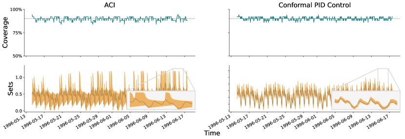
Figure 3: Results for electricity demand forecasting. The left column shows adaptive conformal inference (ACI), and the right column shows conformal PID control. The base forecaster is a Transformer model, and we use a tan integrator and a Theta scorecaster. The format of the figure follows that of Figure 2, except the nominal coverage is now $1-\alpha=0.9$, and the coverage is averaged over a trailing window of 50 points (we also omit the red dots which mark miscoverage events). Summary statistics are available in Table 2.

The results are shown in the right panel of Figure 3, where adaptive conformal inference (ACI) [GC21] is also compared in the left panel. In short, conformal PID control is able to anticipate intraday variations in the scores, and produces sets that “hug” the ground truth sequence tightly; it achieves tight coverage without generating excessively large or infinite sets. The main reason why this is improved is that the scorecaster has a seasonality component built into its prediction model; in general, large improvements such as the one exhibited in Figure 3 should only be expected when the base forecaster is imperfect, as is the case here.

1.3 Related work

The adversarial online view of conformal prediction was pioneered by [GC21] in the same paper that first introduced ACI. Since then, there has been significant work towards improving ACI, primarily by setting the learning rate adaptively [GC22, ZFG⁺22, BWXB23], and incorporating ideas from multicalibration to improve conditional coverage [BGJ⁺22]. It is worth noting that [BWXB23] also makes the observation that the ACI iteration can be generalized to track the quantile of the score sequence, although their focus is on adaptive regret guarantees. Because the topic of adaptive learning rates for ACI and related algorithms has already been investigated heavily, we do not consider it in the current paper. Any such method, such as those of [GC22, BWXB23] should work well in conjunction with our proposed algorithms.

A related but distinct line of work surrounds online calibration in the adversarial sequence model, which dates back to [Fos99, FV98], and connects in interesting ways to both game theory and online learning. We will not attempt to provide a comprehensive review of this rich and sizeable literature, but simply highlight [KL15, KE17, KD23] as a few interesting examples of recent work.

Lastly, outside the online setting, we note that several researchers have been interested in generalizing conformal prediction beyond the i.i.d. (or exchangeable) data setting: this includes [TBCR19, PR21, LC21, FBA⁺22, CLR23], and for time series prediction, in particular, [CWY18, SAvdS21, XX21, XX23, AGKH23]. The focus of all of these papers is quite different, and they all rely on probabilistic assumptions on the data sequence to achieve validity.

2 Methods

We describe the main components of our proposal one at a time, beginning with the quantile tracker.

2.1 Quantile tracking

The starting point for quantile tracking is to consider the following optimization problem:

$$\mathop{\mathrm{minimize}}_{q\in\mathbb{R}}\;\sum_{t=1}^{T}\rho_{1-\alpha}(s_{t}-q),$$ (6)

for large $T$, where we abbreviate $s_{t}=s_{t}(x_{t},y_{t})$ for the score of the test point, and $\rho_{1-\alpha}$ denotes the quantile loss at the level $1-\alpha$, i.e., $\rho_{\tau}(z)=\tau|z|$ for $z>0$ and $(1-\tau)|z|$ for $z\leq 0$. The latter is the standard loss used in quantile regression [KB78, Koe05]. Problem (6) is thus a simple convex (linear) program that tracks the $1-\alpha$ quantile of the score sequence $s_{t}$, $t\in N$. To see this, recall that for a continuously distributed random variable $Z$, the expected loss $\mathbb{E}[\rho_{1-\alpha}(Z-q)]$ is uniquely minimized (over $q\in\mathbb{R}$) at the level $1-\alpha$ quantile of the distribution of $Z$.

In the sequential setting, where we receive one score $s_{t}$ at a time, a natural and simple approach is to apply online gradient descent to (6), with a constant learning rate $\eta>0$. This results in the update:

$$q_{t+1} =q_{t}+\eta\nabla\rho_{1-\alpha}(s_{t}-q_{t})$$

$$=q_{t}+\eta(\mathrm{err}_{t}-\alpha),$$ (7)

where the second line follows as $\nabla\rho_{1-\alpha}(s_{t}-q_{t})=1-\alpha$ if $s_{t}>q_{t}\iff\mathrm{err}_{t}=1$, and $\nabla\rho_{1-\alpha}(s_{t}-q_{t})=-\alpha$ if $s_{t}\leq q_{t}\iff\mathrm{err}_{t}=0$. Note that the update in (7) is highly intuitive: if we miscovered (committed an error) at the last iteration then we increase the quantile, whereas if we covered (did not commit an error) then we decrease the quantile.

Even though it is extremely simple, the quantile tracking iteration (7) can achieve long-run coverage own its own, provided the scores are bounded.

Proposition 1.

Let $\{s_{t}\}_{t\in\mathbb{N}}$ be any sequence of numbers in $[-b,b]$, for $0<b<\infty$. Then the quantile tracking iteration (7) satisfies

$$\Bigg{|}\frac{1}{T}\sum_{t=1}^{T}(\mathrm{err}_{t}-\alpha)\Bigg{|}\leq\frac{b+\eta}{\eta T},$$

for any learning rate $\eta>0$ and $T\geq 1$. In particular, this means (7) yields long-run coverage as in (2).

The proof is very simple, and we derive it as a corollary of Proposition 2, given in the next subsection, because the proof reveals something perhaps unforeseen about the quantile tracker: it acts as an error integrator, despite only adjusting the quantile based on the most recent time step.

Proof.

Without a loss of generality, set $q_{1}=0$. Unraveling the iteration (7) yields

$$q_{t+1}=\eta\sum_{i=1}^{t}(\mathrm{err}_{i}-\alpha).$$ (8)

For $r_{t}(x)=\eta x$, $h(t)=b$, we see (4) holds with $c=1/\eta$. Proposition 2 now applies. ∎

A few remarks are in order. First, although Proposition 1 assumes boundedness of the scores, we do not need to know this bound in order to run (7) and obtain long-run coverage. As long as the scores lie in $[-b,b]$ for any finite $b$, the guarantee goes through—clearly, the quantile tracker proceeds agnostically and performs the same updates in any case.

Second, for the learning rate, in practice we typically set $\eta$ heuristically, as some fraction of the highest score over a trailing window $\hat{B}_{t}=\max\{s_{t-\Delta+1},\dots,s_{t}\}$. On this scale, setting $\eta=0.1\hat{B}_{t}$ usually gives good results, and we use it in all experiments unless specified otherwise (we also set the window length $\Delta$ to be the same as the length of the burn-in period for training the initial base forecaster and scorecaster). Extremely high learning rates result in volatile sets, while very low ones may fail to keep up with rapid changes in the score distribution.

Finally, the proof reveals that quantile tracking (7), which comes from applying online gradient descent to (6), can be equivalently viewed as a pure linear integrator (8) of past coverage errors. This explains why quantile tracking is able to achieve coverage: as we will see later, an error integrator induces a certain kind of self-correcting behavior: after some amount of excess cumulative miscoverage it forces a coverage event, and vice versa, for excess cumulative coverage.

ACI as a special case.

Though it may not be immediately obvious, adaptive conformal inference (ACI) is actually a special case of the quantile tracker. ACI follows the iteration:

$$\alpha_{t+1}=\alpha_{t}-\eta(\mathrm{err}_{t}-\alpha),$$

which is equivalent to

$$1-\alpha_{t+1} =1-\alpha_{t}+\eta(\mathrm{err}_{t}-\alpha)$$

$$=1-\alpha_{t}+\eta\nabla\rho_{1-\alpha}(\beta_{t}-(1-\alpha_{t})),$$

for $\beta_{t}=\inf\{\beta:s_{t}\leq\mathrm{Quantile}_{\beta}\left(\{s_{1},\dots,s_{t-1}\}\right)$. This shows that ACI is a particular instance of the quantile tracker that uses a secondary score $s^{\prime}_{t}=\beta_{t}$ and quantile $q^{\prime}_{t}=1-\alpha_{t}$. Thus, because quantile tracking (7) is the same as a linear coverage integrator (8), so is ACI.

We can see here that ACI transforms unbounded score sequences into bounded ones, which then implies long-run coverage for any score sequence. This may, however, come at a cost: ACI can sometimes output infinite or null prediction sets (when $\alpha_{t}$ drifts below 0 or above 1, respectively). Direct quantile tracking on the scale of the original score sequence does not have this behavior.

2.2 Error integration

Error integration is a generalization of quantile tracking that follows the iteration:

$$q_{t+1}=r_{t}\Bigg{(}\sum_{i=1}^{t}(\mathrm{err}_{i}-\alpha)\Bigg{)},$$ (9)

where $r_{t}$ is a saturation function that satisfies (4) for an admissible function $h$; recall that we use admissible to mean nonnegative, nondecreasing, and sublinear. As we saw in (8), the quantile tracker uses a constant threshold function $h$, whereas $h$ is now permitted to grow, as long as it grows sublinearly, i.e., $h(t)/t\to 0$ as $t\to\infty$. A non-constant threshold function $h$ can be desirable because it means that $r_{t}$ will “saturate” (will hit the conditions on the right-hand sides in (4)) less often, so corrections for coverage error will occur less often, and in this sense, a greater degree of coverage error can be tolerated along the sequence.

The next proposition, in particular its proof, makes the role of $h$ precise.

Proposition 2.

Let $\{s_{t}\}_{t\in\mathbb{N}}$ be any sequence of numbers in $[-b,b]$, where $b>0$, and may be infinite. Assume that $r_{t}$ satisfies (4), for an admissible function $h$. Then the error integration iteration (9) satisfies

$$\Bigg{|}\frac{1}{T}\sum_{t=1}^{T}(\mathrm{err}_{t}-\alpha)\Bigg{|}\leq\frac{ch(T)+1}{T},$$ (10)

for any $T\geq 1$, where $c$ is the constant in (4). In particular, this means (9) yields long-run coverage (2).

Proof of Proposition 2.

Abbreviate $E_{T}=\sum_{t=1}^{T}(\mathrm{err}_{t}-\alpha)$. We will prove one side of the absolute inequality in (10), namely, $E_{T}\leq ch(T)+1$, and the other side follows similarly. We use induction. The base case, for $T=1$, holds trivially. Now assume the result is true up to $T-1$. We divide the argument into two cases: either $ch(T-1)<E_{T-1}\leq ch(T-1)+1$ or $E_{T-1}\leq ch(T-1)$. In the first case, note that that (4) implies $q_{T}=r_{t}(E_{T-1})\geq b$ and therefore $s_{T}\leq q_{T}$ and $\mathrm{err}_{t}=0$. This means that

$$E_{T}=E_{T-1}-\alpha\leq ch(T-1)+1-\alpha\leq ch(T)+1,$$

as $h$ is nondecreasing, which is the desired result at $T$. In the second case, we just use $\mathrm{err}_{T}\leq 1$, so

$$E_{T}\leq E_{T-1}+1-\alpha\leq ch(T-1)+1-\alpha\leq ch(T)+1.$$

This again gives the desired result at $T$, and completes the proof. ∎

Importantly, Proposition 2 suffices to prove Theorem 1.

Proof of Theorem 1.

We can transform (5) by setting $q^{\prime}_{t+1}=q_{t+1}-\hat{q}_{t+1}$, and this becomes an update of the form (9) with respect to $q^{\prime}_{t+1}$. Further, the score sequence in this new parameterization is $s^{\prime}_{t}=s_{t}-\hat{q}_{t}$, which is in $[-b,b]$ because both $s_{t}$ and $\hat{q}_{t}$ are in $[-b/2,b/2]$. Applying Proposition 2 gives the result. ∎

As already mentioned in the introduction, in all our experiments we use a nonlinear saturation function $r_{t}(x)=K_{\text{I}}\tan(x\log(t)/(tC_{\text{sat}}))$, where we set $\tan(x)=\mathrm{sign}(x)\cdot\infty$ for $x\notin[-\pi/2,\pi/2]$, and $C_{\text{sat}},K_{\text{I}}>0$ are constants that we choose heuristically (described in Appendix B). In a sense, this tan integrator is akin to a quantile tracker whose learning rate adapts to the current coverage gap. To see this, we can use a first-order Taylor approximation, which shows (ignoring constants):

$$q_{t+1}=\tan\Bigg{(}\frac{\log(t)}{t}\sum_{i=1}^{t}(\mathrm{err}_{i}-\alpha)\Bigg{)}\approx q_{t}+\underbrace{\frac{\log(t)}{t}\sec^{2}\Bigg{(}\frac{\log(t-1)}{t-1}\sum_{i=1}^{t-1}(\mathrm{err}_{i}-\alpha)\Bigg{)}}_{\text{effective learning rate}}\nabla\rho_{1-\alpha}(s_{t}-q_{t}).$$

Above, $\sec(x)=1/\cos(x)$ is the secant function, which has a U-shape; thus we can see from the above that the effective learning rate is higher for larger errors. Similar analyses for different integrators will give different adaptive learning rates; see Appendix C for another example.

2.3 Scorecasting

The final piece to discuss is scorecasting. A scorecaster attempts to forecast $q_{t+1}$ directly, taking advantage of any leftover signal that is not captured by the base forecaster. This is the role played by $\hat{q}_{t+1}$ in (5). Scorecasting may be particularly useful when it is difficult to modify or re-train the base forecaster. This can occur when the base forecaster is computationally costly to train (e.g., as in a Transformer model); or it can occur in complex operational prediction pipelines where frequently updating a forecasting implementation is infeasible. Another scenario where scorecasting may be useful is one in which the forecaster and scorecaster have access to different levels of data. For example, if a public health agency collects epidemic forecasts from external groups, and forms an ensemble forecast, then the agency may have access to finer-grained data that it can use to recalibrate the ensemble’s prediction sets (compared to the level of data granularity granted to the forecasters originally).

This motivates the need for scorecasting as a modular layer that “sits on top” of the base forecaster and residualizes out systematic errors in the score distribution. This intuition is made more precise by recalling, as described above (following Proposition 2), that scorecasting combined with error integration as in (5) is just a reparameterization of error integration (9), where $q^{\prime}_{t}=q_{t}-\hat{q}_{t}$ and $s^{\prime}_{t}=s_{t}-\hat{q}_{t}$ are the new quantile and new score, respectively. A well-executed scorecaster could reduce the variability in the scores and make them more exchangeable, resulting in more stable coverage and tighter prediction sets, as seen in Figure 3. On the other hand, using an aggressive scorecaster in a situation in which there is little or no signal left in the scores can actually hurt: in this case it would only add variance to the new score sequence $s^{\prime}_{t}$, which could result in more volatile coverage and larger sets.

There is no limit to what we can choose for the scorecasting model. We might like to use a model that can simultaneously incorporate seasonality, trends, and exogenous covariates. Two traditional choices would be SARIMA (seasonal autoregressive integrated moving average) and ETS (error-trend-seasonality) models, but there are many other available methods, such as the Theta model [AN00], Prophet model [TL18], and various neural network forecasters. A modern review of forecasting methods is given in [HA18].

2.4 Putting it all together

Briefly, we revisit the PID perspective, to recap how quantile tracking, error integration, and scorecasting fit in and work in combination. It helps to return to (3), which we copy again here for convenience:

$$q_{t+1}=g^{\prime}_{t}+\eta(\mathrm{err}_{t}-\alpha)+r_{t}\Bigg{(}\sum_{i=1}^{t}(\mathrm{err}_{i}-\alpha)\Bigg{)}.$$ (11)

Quantile tracking is precisely given by taking $g^{\prime}_{t}=q_{t}$ and $r_{t}=0$. This can be seen as equivalent to P control: subtract $q_{t}$ from both sides in (11) and treat the increment $u_{t+1}=q_{t+1}-q_{t}$ as the process variable; then in this modified system, quantile tracking is exactly P control. For this reason, we use “conformal P control” to refer to the quantile tracker in the experiments that follow. Similarly, we use “conformal PI control” to refer to the choice $g^{\prime}_{t}=q_{t}$, and $r_{t}\not=0$ as a generic integrator (for us, tan is the default). Lastly, “conformal PID control” refers to letting $g^{\prime}_{t}$ be a generic scorecaster, and $r_{t}\not=0$ be a generic integrator.

3 Experiments

In addition to the statewide COVID-19 death forecasting experiment described in the introduction, we run experiments on all combinations of the following data sets and forecasters.

Data sets:

• Electricity demand in New South Wales [Har99]

• Return (log price) of Amazon, Google, and Microsoft stock [Ngu18]

• Temperature in Delhi [Vra17]

Forecasters (all via darts [HLP⁺22]) :

• Autoregressive (AR) model with 3 lags

• Theta model with $\theta=2$ [AN00]

• Prophet model [TL18]

• Transformer model [VSP⁺17]

In all cases except for the COVID-19 forecasting data set, we: re-train the base forecaster at each time point; construct prediction sets using the asymmetric (signed) residual score; and use a Theta model for the scorecaster. For the COVID-19 forecasting setting, we: use the given ensemble model as the base forecaster (no training at all); construct prediction sets using the asymmetric quantile score; and use an $\ell_{1}$-penalized quantile regression as the scorecaster, fit on features derived from previous forecasts, cases, and deaths, as described in the introduction. And lastly, in all cases, we use a tan function for the integrator with constants chosen heuristically, as described in Appendx B.

The results that we choose to show in the subsections below are meant to illustrate key conceptual points (differences between the methods). Additional results are presented in Appendix F. Our GitHub repository, https://github.com/aangelopoulos/conformal-time-series, provides the full suite of evaluations.

3.1 ACI versus quantile tracking

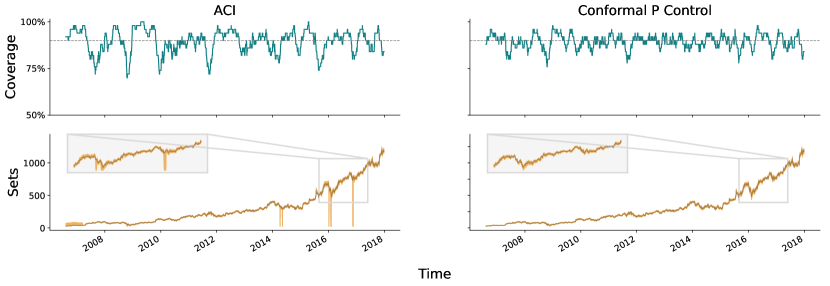
	AR		Prophet		Theta		Transformer
	ACI	P Ctrl	ACI	P Ctrl	ACI	P Ctrl	ACI	P Ctrl
Marginal coverage	0.894	0.894	0.904	0.888	0.895	0.894	0.906	0.887
Longest err sequence	6	3	13	6	5	5	21	9
Average set size	$\infty$	17.6	$\infty$	51.7	$\infty$	17.8	$\infty$	70.4
Median set size	13.4	13.3	50.7	37.3	12.8	13.1	61.9	44.3
75% quantile set size	28.4	22.3	117	72.1	20.9	22.6	179	98.4
90% quantile set size	44.1	37.7	236	114	38.6	38.4	302	153
95% quantile set size	49.9	46.2	$\infty$	140	48.2	46.9	$\infty$	196

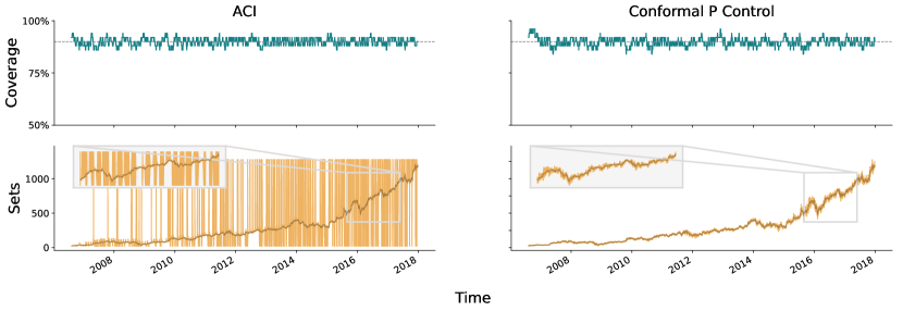
Figure 4: Results for forecasting Amazon stock return, comparing ACI and quantile tracking (P control). The plots show AR as the base forecaster; the table summarizes the results of all four base forecasters. We use the default learning rates for both ACI and quantile tracking: $\eta=0.005$ and $\eta=0.1\hat{B}_{t}$, respectively.

	AR		Prophet		Theta		Transformer
	ACI	P Ctrl	ACI	P Ctrl	ACI	P Ctrl	ACI	P Ctrl
Marginal coverage	0.9	0.898	0.901	0.897	0.9	0.896	0.902	0.897
Longest err sequence	2	2	8	3	2	2	7	3
Average set size	$\infty$	28.4	$\infty$	42.6	$\infty$	27.8	$\infty$	54.2
Median set size	$\infty$	18.6	60.6	31.9	$\infty$	18.7	46	35.5
75% quantile set size	$\infty$	37.4	$\infty$	56.5	$\infty$	37.8	$\infty$	69.7
90% quantile set size	$\infty$	66.3	$\infty$	93.4	$\infty$	63.4	$\infty$	123
95% quantile set size	$\infty$	81.8	$\infty$	116	$\infty$	78.5	$\infty$	164

Figure 5: As in Figure 5, but with larger learning rates for ACI and quantile tracking: $\eta=0.1$ and $\eta=0.5\hat{B}_{t}$, respectively.

We forecast the daily Amazon (AMZN) opening stock price from 2006–2014. We do this in log-space (hence predicting the return of the stock). Figure 5 compares ACI and the quantile tracker, each with its default learning rate: $\eta=0.005$ for ACI, and $\eta=0.1\hat{B}_{t}$ for quantile tracking. We see that the coverage from each method is decent, but oscillates nontrivially around the nominal level of $1-\alpha=0.9$ (with ACI generally having larger oscillations). Figure 5 thus increases the learning rate for each method: $\eta=0.1$ for ACI, and $\eta=0.5\hat{B}_{t}$ for the quantile tracker. We now see that both deliver very tight coverage. However, ACI does so by frequently returning infinite sets; meanwhile, the corrections to the sets made by the quantile tracker are nowhere near as aggressive.

As a final comparison, in Appendix D, we modify ACI to clip the sets in a way that disallows them from ever being infinite. This heuristic may be used by practitioners that want to guard against infinite sets, but it no longer has a validity guarantee for bounded or unbounded scores. The results in the appendix indicate that the quantile tracker has similar coverage to this procedure, and usually with smaller sets.

3.2 The effect of integration

Next we forecast the daily Google (GOOGL) opening stock price from 2006–2014 (again done in log-space). Figure 6 compares the quantile tracker without and without an additional integrator component (P control versus PI control). We purposely choose a very small learning rate, $\eta=0.01\hat{B}_{t}$, in order to show how the integrator can stabilize coverage, which it does nicely for most of the time series. The coverage of PI control begins to oscillate more towards the end of the sequence, which we attribute at least in part to the fact that the integrator measures coverage errors accumulated over all time—and by the end of a long sequence, the marginal coverage can still be close to $1-\alpha$ even if the local coverage deviates more wildly. This can be addressed by using a local version of the integrator, an idea we return to in the discussion.

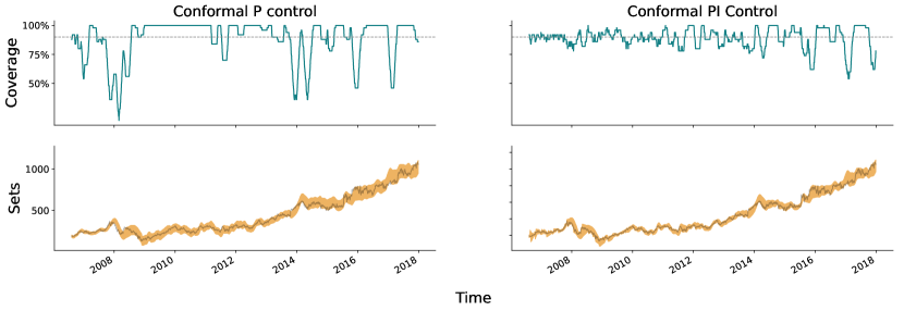
	AR		Prophet		Theta		Transformer
	P Ctrl	PI Ctrl	P Ctrl	PI Ctrl	P Ctrl	PI Ctrl	P Ctrl	PI Ctrl
Marginal coverage	0.895	0.896	0.882	0.888	0.891	0.896	0.817	0.897
Longest err sequence	6	3	31	13	58	6	106	10
Average set size	19.2	24.7	95.6	68.2	42.9	33.5	281	108
Median set size	16.4	22.8	91.5	60.7	44.3	32.8	219	73.8
75% quantile set size	21.3	30.1	120	88	60	42.6	386	121
90% quantile set size	30.7	38.4	150	118	66.2	51.3	482	244
95% quantile set size	32.8	44.7	156	139	69.1	57.5	524	341

Figure 6: Results for forecasting Google stock return, comparing quantile tracking with and without the integrator (P control versus PI control). The plots show Prophet as the base forecaster; the table summarizes the results of all four base forecasters. We purposely use a very small learning rate, $\eta=0.01\hat{B}_{t}$, in order to show how the integrator can stabilize coverage.

3.3 The effect of scorecasting

Figures 2 and 3 already showcase examples in which scorecasting offers significant improvement in coverage and set sizes. Recall that these were settings in which the base forecaster produces errors (scores) that have predictable trends. Further examples in the COVID-19 forecasting setting, which display similar benefits to scorecasting, are given in Appendix E.

We emphasize that it is not always the case that scorecasting will help. In some settings, scorecasting may introduce enough variance into the new score sequence that the coverage or sets will degrade in stability. (For example, this will happen if we run a highly complex scorecaster on a sequence of i.i.d. scores, where there are no trends whatsoever.) In practice, scorecasters should be designed with care, just as one would design a base forecaster; it is unlikely that using “out of the box” techniques for scorecasting will be robust enough, especially in high-stakes problems. Appendix F provides examples in which scorecasting, run across all settings using a generic Theta model, can hurt (for example, it adds noticeable variance to the coverage and sets in some instances within the Amazon data setting).

4 Discussion

Our work presents a framework for constructing prediction sets in time series that is analogous (and indeed formally equivalent) to PID control. The framework consists of quantile tracking (P control), which is simply online gradient descent applied to the quantile loss; error integration (I control) to stabilize coverage; and scorecasting (D control) to remove systematic trends in the scores (errors made by the base forecaster).

We found the combination of quantile tracking and integration to consistently yield robust and favorable performance in our experiments. Scorecasting provides additional benefits if there are trends left in scores that are predictable (and the scorecaster is well-designed), as is the case in some of our examples. Otherwise, scorecasting may add variability and make the coverage and prediction sets more volatile. Overall, designing the scorecaster (which includes the choice to even use one at all) is an important modeling step, just like the design of the base forecaster.

It is worth emphasizing that, with the exception of the COVID-19 forecasting example, our experiments are intended to be illustrative and we did not look to use state-of-the-art forecasters, or include any and all possibly relevant features for prediction. Further, while we found that using heuristics to set constants (such as the learning rate $\eta$, and constants $C_{\text{sat}},K_{\text{I}}$ for the tan integrator) worked decently well, we believe that more rigorous techniques, along the lines of [GC22, BWXB23], can be used to tune these adaptively in an online fashion.

We now present an extension of our analysis to conformal risk control [ABF⁺22, BAL⁺21, FRBR22]. In this problem setting, we are given a sequence of loss functions $L_{t}:2^{\mathcal{Y}}\times\mathcal{Y}\to[0,1]$ satisfying $L_{t}(\mathcal{Y},y)=0$ for all $y$, and $L_{t}(\emptyset,y)=1$ for all $y$. The goal is to bound the deviation of the average risk $\frac{1}{T}\sum_{t=1}^{T}L_{t}(\mathcal{C}_{t},y_{t})$ from $\alpha$. We state a result for the integrator below, and give its proof in Appendix A.

Proposition 3.

Consider the iteration $q_{t+1}=r_{t}(\sum_{i=1}^{t}(L_{i}(\mathcal{C}_{i},y_{i})-\alpha))$, with $L_{t}$ as above. Assume that $r_{t}$ satisfies (4), for an admissible function $h$. Also assume that $C_{t}(\mathcal{C}_{t},y_{t})=\emptyset$ if $q_{t}\leq-b$ and $\mathcal{Y}$ if $q_{t}\geq b$, where $b>0$, and may be infinite. Then for all $T\geq 1$,

$$\Bigg{|}\frac{1}{T}\sum_{t=1}^{T}(L_{t}(\mathcal{C}_{t},y_{t})-\alpha)\Bigg{|}\leq\frac{ch(T)+1}{T}.$$ (12)

for any $T\geq 1$, where $c$ is the constant in (4).

We briefly conclude by mentioning that we believe many other extensions are possible, especially with respect to the integrator. Broadly, we can choose to integrate in a kernel-weighted fashion

$$r_{t}\Bigg{(}\sum_{i=1}^{t}(\mathrm{err}_{i}-\alpha)\cdot K\big{(}(i,x_{i},y_{i}),(t,x_{t},y_{t})\big{)}\Bigg{)}$$ (13)

As a special case, the kernel could simply assign weight 1 if $t-i\leq w$, and weight 0 otherwise, which would result in an integrator that aggregates coverage over a trailing window of length $w$. This can help consistently sustain better local coverage, for long sequences. As another special case, the kernel could assign a weight based on whether $x_{i}$ and $x_{t}$ lie in the same bin in some pre-defined binning of $\mathcal{X}$ space, which may be useful for problems with group structure (where we want group-wise coverage). Many other choices and forms of kernels are possible, and it would be interesting to consider adding together a number of such choices (13) in combination, in a multi-resolution flavor, for the ultimate quantile update.

Appendix A Conformal risk control guarantee

Proof of Proposition 3.

The proof is similar to that of Proposition 2—as in that proof, we only prove one side of the absolute inequality (12), and use induction. Abbreviate $E_{T}=\sum_{t=1}^{T}(L_{i}(\mathcal{C}_{i},y_{i})-\alpha))$. The base case holds trivially. For the inductive step, either $ch(T-1)<E_{T-1}\leq ch(T-1)+1$ or $E_{T-1}\leq ch(T-1)$. In the first case, we have saturated, so $L_{t}(\mathcal{C}_{t},y_{t})=0$, and

$$E_{T}=E_{T-1}-\alpha\leq ch(T-1)+1-\alpha\leq ch(T)+1,$$

as $h$ is nondecreasing, which is the desired result at $T$. In the second case, we just use the boundedness of the loss $L_{t}(\mathcal{C}_{t},y_{t})\leq 1$, so

$$E_{T}\leq E_{T-1}+1-\alpha\leq ch(T-1)+1-\alpha\leq ch(T)+1.$$

This again gives the desired result at $T$, and completes the proof. ∎

Appendix B Heuristics for setting constants

Consider the tan integrator $r_{t}(x)=K_{\text{I}}\tan(x\log(t)/(tC_{\text{sat}}))$, where we set $\tan(x)=\mathrm{sign}(x)\cdot\infty$ whenever $x\notin[-\pi/2,\pi/2]$, and $C_{\text{sat}},K_{\text{I}}>0$ are constants. The constant $C_{\text{sat}}$ is primarily in charge of guaranteeing that by time $T$, we want to have an absolute guarantee of at least $1-\alpha-\delta$ coverage. Then we can set

$$C_{\text{sat}}=\frac{2}{\pi}\big{(}\lceil\log(T)\delta\rceil-1/\log(T)\big{)}$$

to ensure the tan function has an asymptote at the correct point. The purpose of the constant $K_{\text{I}}$ is to place the integrator on the same scale as the scores. So if $B^{\prime}$ is a hypothesized bound on the magnitude of the scores, then one can set $K_{\text{I}}=B^{\prime}$. In practice, these heuristics can be taken as a starting place, and then the numbers can be fine-tuned during a burn-in period by hand or algorithmically. As alluded to previously, we believe there is room for work in the style of [GC22, BWXB23] to rigorously tune these parameters online, but it is not the focus of our paper.

Appendix C Quantile tracking with decaying learning rate

Consider $r_{t}(x)=\eta x/\sqrt{t}$. (This will give long-run coverage only for bounded scores, because condition (4) is only met for finite and not infinite $b$.) Then (9) becomes $q_{t+1}=\frac{\eta}{\sqrt{t}}\sum_{i=1}^{t}(\mathrm{err}_{i}-\alpha)$, which can be rewritten as

$$q_{t+1}=\frac{\sqrt{t-1}}{\sqrt{t}}\frac{\eta}{\sqrt{t-1}}\sum_{i=1}^{t-1}(\mathrm{err}_{i}-\alpha)+\frac{\eta}{\sqrt{t}}(\mathrm{err}_{i}-\alpha)\approx q_{t}+\frac{\eta}{\sqrt{t}}(\mathrm{err}_{t}-\alpha).$$

This is approximately the quantile tracker (7) with a decaying learning rate, on the order of $1/\sqrt{t}$.

Appendix D Comparison to clipped ACI

Figures 8 and 8 compare the quantile tracker to a clipped version of ACI which disallows infinite-sized sets by clipping the sets to the largest score seen so far.

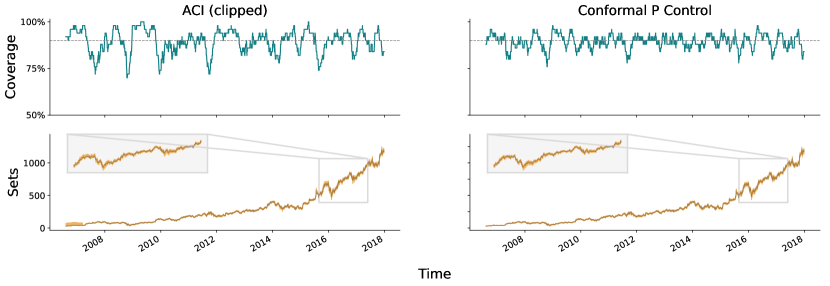
	AR		Prophet		Theta		Transformer
	ACI (clipped)	P Ctrl	ACI (clipped)	P Ctrl	ACI (clipped)	P Ctrl	ACI (clipped)	P Ctrl
Marginal coverage	0.898	0.898	0.884	0.897	0.898	0.896	0.884	0.897
Longest err sequence	2	2	8	3	2	2	7	3
Average set size	44.9	28.4	52.6	42.6	43.3	27.8	60.5	54.2
Median set size	41.8	18.6	38.8	31.9	27.3	18.7	36.6	35.5
75% quantile set size	58.9	37.4	66.9	56.5	59.5	37.8	85.5	69.7
90% quantile set size	93.9	66.3	137	93.4	94.7	63.4	148	123
95% quantile set size	136	81.8	166	116	136	78.5	182	164

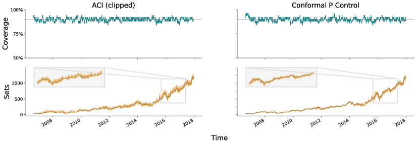
Figure 7: As in Figure 5, but with clipped ACI.

	AR		Prophet		Theta		Transformer
	ACI (clipped)	P Ctrl	ACI (clipped)	P Ctrl	ACI (clipped)	P Ctrl	ACI (clipped)	P Ctrl
Marginal coverage	0.894	0.894	0.896	0.888	0.895	0.894	0.89	0.887
Longest err sequence	6	3	13	6	5	5	21	9
Average set size	19.5	17.6	69.5	51.7	17.9	17.8	115	70.4
Median set size	13.4	13.3	48.7	37.3	12.8	13.1	61.7	44.3
75% quantile set size	27.9	22.3	91.1	72.1	20.7	22.6	165	98.4
90% quantile set size	44	37.7	168	114	38.5	38.4	248	153
95% quantile set size	48.7	46.2	195	140	47.2	46.9	304	196

Figure 8: As in Figure 5, but with clipped ACI.

Appendix E More details on COVID-19 forecasting

In this experiment, the scorecaster receives as input the three most recent scores (i.e., quantile errors) of the ensemble forecaster, as well as the three most recent case and death counts, from all 50 states. The scorecaster is an $\ell_{1}$-penalized quantile regression as implemented by sklearn.linear_model.QuantileRegressor. We fixed tuning parameter for the $\ell_{1}$ penalty at 10; in our experience, the performance of the scorecaster was fairly robust to this choice. Automatic selection (e.g., using cross-validation) could be the topic of future study. Figures 10 and 10 shows the analogous experiments but for forecasting in New York and Texas.

	Base Forecaster	Conformal PID Ctrl
Marginal coverage	0.82	0.86
Longest err sequence	6	2
Average set size	625	858
Median set size	512	688
75% quantile set size	754	1.01e+03
90% quantile set size	1.12e+03	1.47e+03
95% quantile set size	1.45e+03	1.8e+03

Table 1: Summary statistics for COVID-19 death forecasting in California, as in Figure 2.

	AR		Transformer
	ACI	Conformal PID Control	ACI	Conformal PID Ctrl
Marginal coverage	0.899	0.9	0.899	0.901
Longest err sequence	3	2	3	2
Average set size	$\infty$	0.177	$\infty$	0.174
Median set size	0.406	0.178	0.426	0.175
75% quantile set size	0.484	0.21	0.574	0.206
90% quantile set size	0.672	0.236	$\infty$	0.233
95% quantile set size	$\infty$	0.252	$\infty$	0.249

Table 2: Summary statistics for electricity forecasting, as in Figure 3. Results for the Prophet and Theta models are not available because darts does not support intermittent retraining for these algorithms.

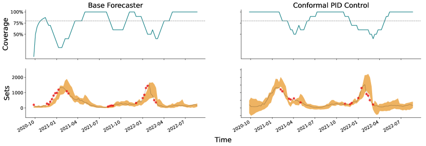
	Base Forecaster	Conformal PID Ctrl
Marginal coverage	0.78	0.85
Longest err sequence	8	3
Average set size	310	472
Median set size	249	440
75% quantile set size	388	608
90% quantile set size	667	821
95% quantile set size	754	1.03e+03

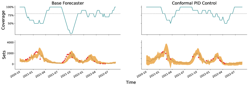
Figure 9: Results for 4-week ahead COVID-19 death forecasting in New York.

	Base Forecaster	Conformal PID Ctrl
Marginal coverage	0.75	0.85
Longest err sequence	7	2
Average set size	556	827
Median set size	482	706
75% quantile set size	759	1.03e+03
90% quantile set size	993	1.36e+03
95% quantile set size	1.11e+03	1.57e+03

Figure 10: Results for 4-week ahead COVID-19 death forecasting in Texas.

Appendix F Further experiments

We give a more comprehensive view of our results, examing all data sets, and a range of tuning parameters for each method. We restrict our attention to AR as the base forecaster; for the rest of the base forecasters, we refer to the GitHub repository: https://github.com/aangelopoulos/conformal-time-series.

For each experiment, we describe the data set in a new subsection, and two plots are included: one for the coverage, and one for the prediction sets. Each column in the plots represents a different method, and each row is a different learning rate. For the quantile tracker, the learning rate is to be interpreted as the multiplier in front of $\hat{B}_{t}$. Each method is given a different color, which stays consistent throughout the plots. We use a tan integrator and a Theta scorecaster throughout, just as in the main text experiments.

F.1 Amazon/Google

These data sets are part of a multivariate time series consisting of thirty blue-chip stock prices, including those of Amazon (AMZN) and Google (GOOGL), from January 1, 2006 to December 31, 2014. We attempt to forecast the daily opening price of each of Amazon and Google stock, on a log scale. Available to the scorecaster are the previous open prices of all 30 stocks.

F.2 Microsoft

This data set is a univariate time series consisting of a single stock open price, that of Microsoft (MSFT), from April 1, 2015 to May 31, 2021.

F.3 Daily temperature in Delhi

This data set contains the daily temperature (averaged over 8 measurements in 3 hour periods), humidity, wind speed, and atmospheric temperature in the city of Delhi from January 1, 2003 to April 24, 2017, scraped using the Weather Underground API.

F.4 Electricity demand forecasting

This data set measures electricity demand in New South Wales collected at half-hour increments from May 7th, 1996 to December 5th, 1998 (we zoom in on the first 2000 time points). There are also several other variables collected, such as the demand and price in Victoria, the amount of energy transfer between New South Wales and Victoria, and so on. These are given as covariates to the scorecaster. The demand value is normalized by default to lie in $[0,1]$.

F.5 Synthetic data sets

We perform some experiments on two synthetic score sequences which include change points and other behaviors difficult to produce using real data. In this setting, there is no ground truth $y_{t}$ sequence, so we do not plot the sets. Instead, we plot the scores themselves in one column, and the quantiles $q_{t}$ produced by each algorithm in a different column (when $q_{t}\geq s_{t}$, we cover). The general goal is for $q_{t}$ to track the $1-\alpha$ quantile of $s_{t}$, and if it is too far off, that corresponds to the “set being too large or too small” in a situation where we would be constructing sets out of these scores.

We consider an i.i.d. sequence of scores, a noisy increasing sequence of scores, and a mix of change points and trends. Our codebase describes the score generation procedure in more detail.

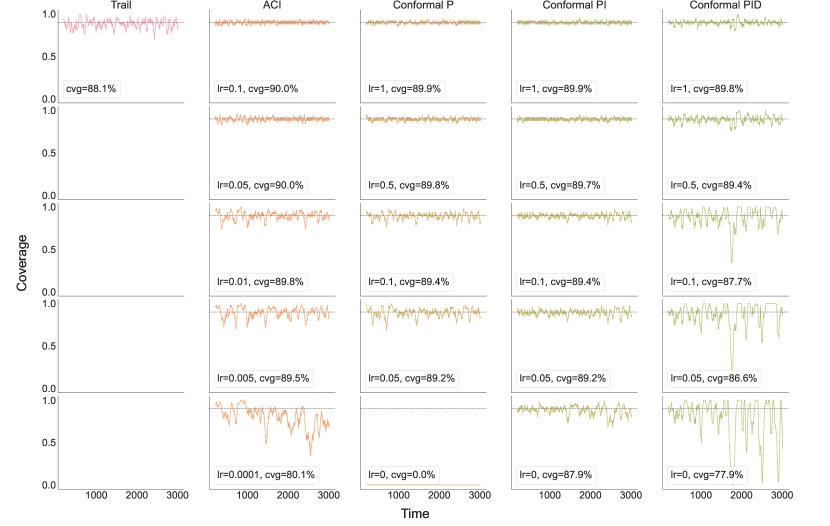
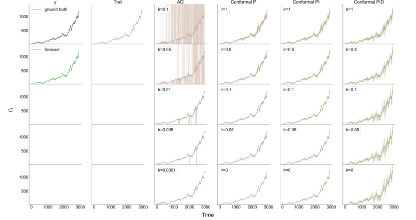
Figure 11: Results for the Amazon data set.

Figure 12: Results for the Google data set.

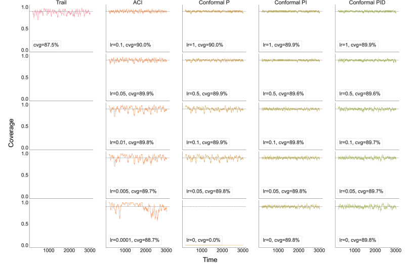
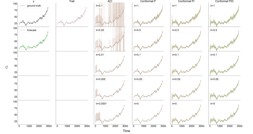
Figure 13: Results for the Microsoft data set.

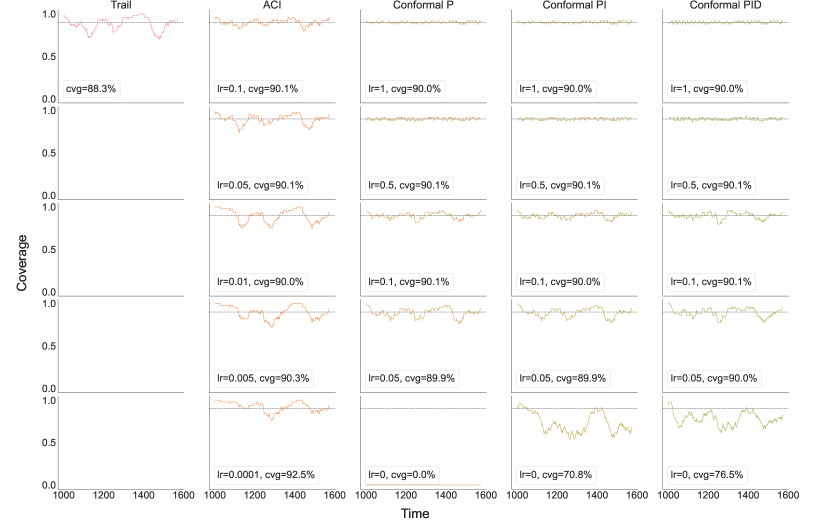
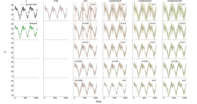
Figure 14: Results for the Delhi temperature data set.

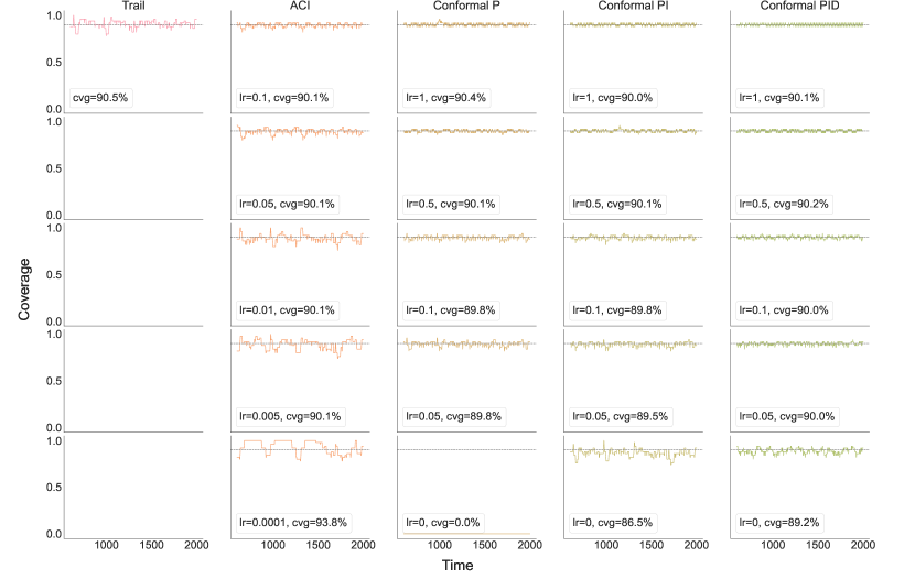
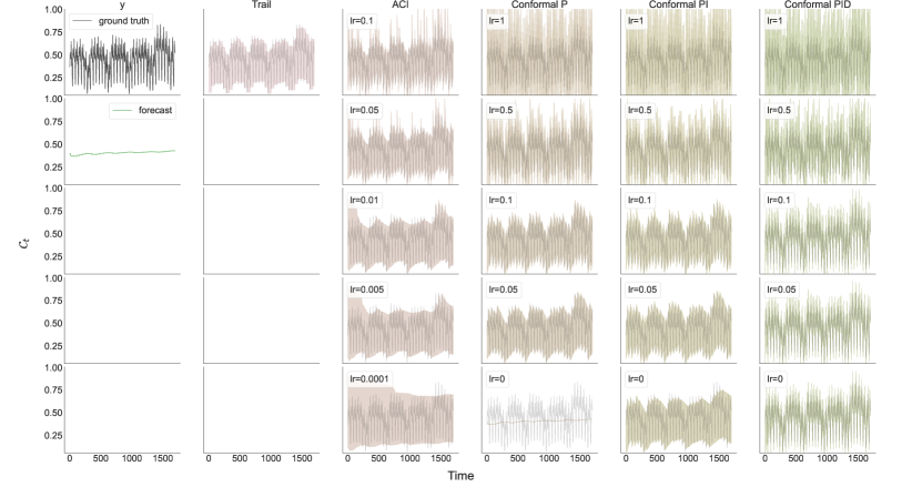
Figure 15: Results for the electricity demand forecasting data set.

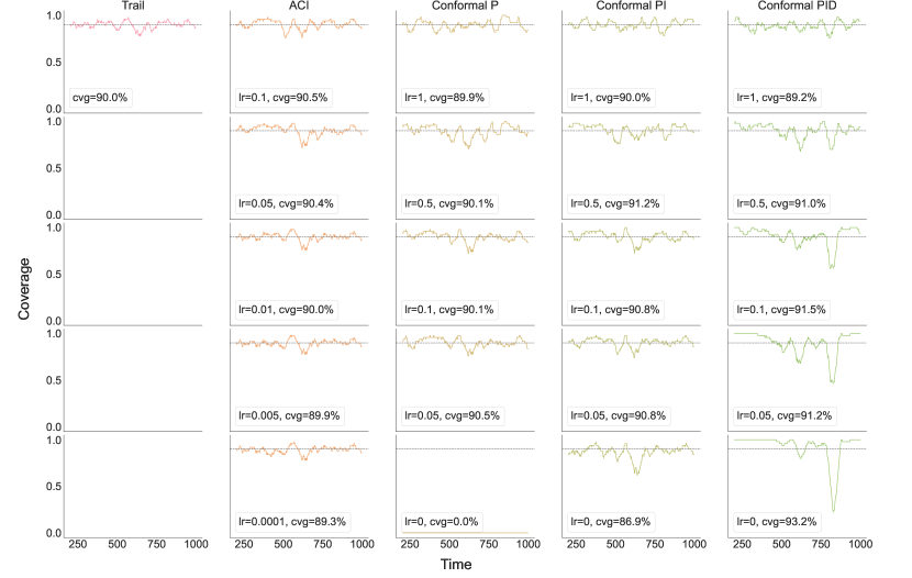
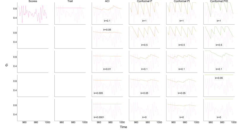
Figure 16: Results for an i.i.d. score sequence.

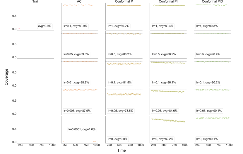
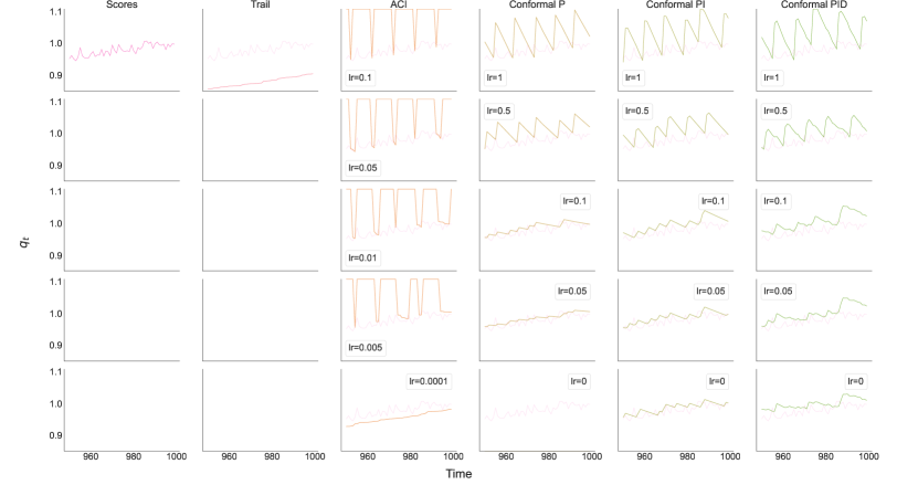
Figure 17: Results for an increasing score sequence.

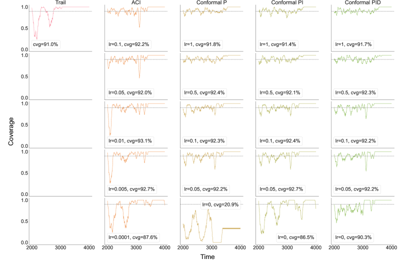
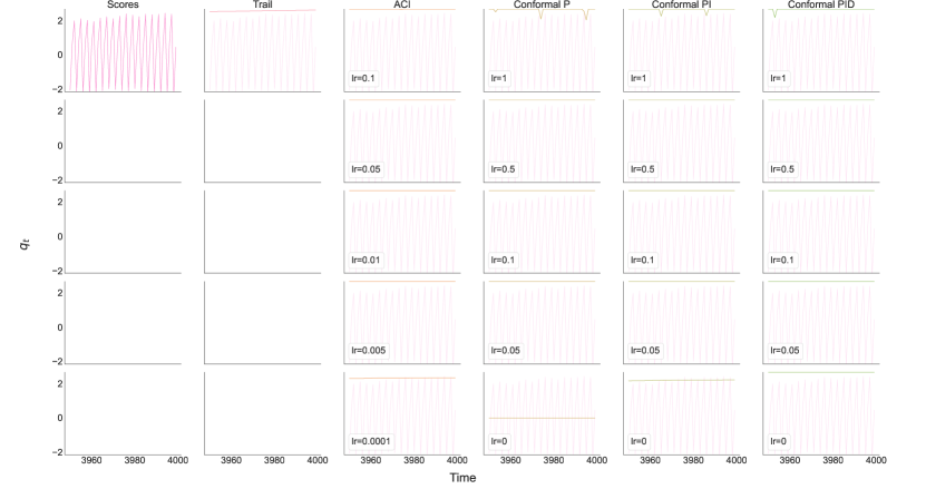
Figure 18: Results for a score sequence that is a mix of change points and trends.

References

- [ABF+22] Anastasios N. Angelopoulos, Stephen Bates, Adam Fisch, Lihua Lei, and Tal Schuster. Conformal risk control. arXiv preprint arXiv:2208.02814, 2022.
- [AGKH23] Andreas Auer, Martin Gauch, Daniel Klotz, and Sepp Hochreiter. Conformal prediction for time series with modern Hopfield networks. arXiv preprint arXiv:2303.12783, 2023.
- [AN00] Vassilis Assimakopoulos and Konstantinos Nikolopoulos. The theta model: A decomposition approach to forecasting. International Journal of Forecasting, 16(4):521–530, 2000.
- [BAL+21] Stephen Bates, Anastasios Angelopoulos, Lihua Lei, Jitendra Malik, and Michael I. Jordan. Distribution-free, risk-controlling prediction sets. Journal of the ACM, 68(6):1–34, 2021.
- [BGJ+22] Osbert Bastani, Varun Gupta, Christopher Jung, Georgy Noarov, Ramya Ramalingam, and Aaron Roth. Practical adversarial multivalid conformal prediction. In Advances in Neural Information Processing Systems, 2022.
- [BWXB23] Aadyot Bhatnagar, Huan Wang, Caiming Xiong, and Yu Bai. Improved online conformal prediction via strongly adaptive online learning. arXiv preprint arXiv:2302.07869, 2023.
- [CHW+22] Estee Y. Cramer, Yuxin Huang, Yijin Wang, Evan L. Ray, Matthew Cornell, Johannes Bracher, Andrea Brennen, Alvaro J. Castro Rivadeneira, Aaron Gerding, Katie House, Dasuni Jayawardena, Abdul Hannan Kanji, Ayush Khandelwal, Khoa Le, Vidhi Mody, Vrushti Mody, Jarad Niemi, Ariane Stark, Apurv Shah, Nutcha Wattanchit, Martha W. Zorn, Nicholas G. Reich, and US COVID-19 Forecast Hub Consortium. The United States COVID-19 Forecast Hub dataset. Scientific Data, 9, 2022.
- [CLR23] Emmanuel J. Candès, Lihua Lei, and Zhimei Ren. Conformalized survival analysis. Journal of the Royal Statistical Society: Series B, 85(1):24–45, 2023.
- [CRL+22] Estee Y. Cramer, Evan L. Ray, Velma K. Lopez, Johannes Bracher, Andrea Brennen, Alvaro J. Castro Rivadeneira, Aaron Gerding, Tilmann Gneiting, Katie H. House, Yuxin Huang, Dasuni Jayawardena, Abdul H. Kanji, Ayush Khandelwal, Khoa Le, Anja Mühlemann, Jarad Niemi, Apurv Shah, Ariane Stark, Yijin Wang, Nutcha Wattanachit, Martha W. Zorn, Youyang Gu, Sansiddh Jain, Nayana Bannur, Ayush Deva, Mihir Kulkarni, Srujana Merugu, Alpan Raval, Siddhant Shingi, Avtansh Tiwari, Jerome White, Spencer Woody, Maytal Dahan, Spencer Fox, Kelly Gaither, Michael Lachmann, Lauren Ancel Meyers, James G. Scott, Mauricio Tec, Ajitesh Srivastava, et al. Evaluation of individual and ensemble probabilistic forecasts of COVID-19 mortality in the United States. Proceedings of the National Academy of Sciences, 119(15):e2113561119, 2022.
- [CWY18] Victor Chernozhukov, Kaspar Wuthrich, and Zhu Yinchu. Exact and robust conformal inference methods for predictive machine learning with dependent data. In Proceedings of the Annual Conference on Learning Theory, 2018.
- [FBA+22] Clara Fannjiang, Stephen Bates, Anastasios N. Angelopoulos, Jennifer Listgarten, and Michael I. Jordan. Conformal prediction under feedback covariate shift for biomolecular design. Proceedings of the National Academy of Sciences, 119(43):e2204569119, 2022.
- [Fos99] Dean P Foster. A proof of calibration via Blackwell’s approachability theorem. Games and Economic Behavior, 29(1-2):73–78, 1999.
- [FRBR22] Shai Feldman, Liran Ringel, Stephen Bates, and Yaniv Romano. Achieving risk control in online learning settings. arXiv preprint arXiv:2205.09095, 2022.
- [FV98] Dean P. Foster and Rakesh V. Vohra. Asymptotic calibration. Biometrika, 85(2):379–390, 1998.
- [GC21] Isaac Gibbs and Emmanuel J. Candès. Adaptive conformal inference under distribution shift. In Advances in Neural Information Processing Systems, 2021.
- [GC22] Isaac Gibbs and Emmanuel J. Candès. Conformal inference for online prediction with arbitrary distribution shifts. arXiv preprint arXiv:2208.08401, 2022.
- [HA18] Rob J. Hyndman and George Athanasopoulos. Forecasting: Principles and Practice. OTexts, 2018.
- [Har99] Michael Harries. Splice-2 comparative evaluation: Electricity pricing. Technical report, University of New South Wales, 1999.
- [HLP+22] Julien Herzen, Francesco Lässig, Samuele Giuliano Piazzetta, Thomas Neuer, Léo Tafti, Guillaume Raille, Tomas Van Pottelbergh, Marek Pasieka, Andrzej Skrodzki, Nicolas Huguenin, Maxime Dumonal, Jan Kościsz, Dennis Bader, Frédérick Gusset, Mounir Benheddi, Camila Williamson, Michal Kosinski, Matej Petrik, and Gaël Grosch. Darts: User-friendly modern machine learning for time series. Journal of Machine Learning Research, 23(1):5442–5447, 2022.
- [KB78] Roger Koenker and Gilbert Bassett. Regression quantiles. Econometrica, 46(1):33–50, 1978.
- [KD23] Volodymyr Kuleshov and Shachi Deshpande. Online calibrated regression for adversarially robust forecasting. arXiv preprint arXiv:2302.12196, 2023.
- [KE17] Volodymyr Kuleshov and Stefano Ermon. Estimating uncertainty online against an adversary. In Association for the Advancement of Artificial Intelligence, 2017.
- [KL15] Volodymyr Kuleshov and Percy Liang. Calibrated structure prediction. In Advances in Neural Information Processing Systems, 2015.
- [Koe05] Roger Koenker. Quantile Regression. Cambridge University Press, 2005.
- [LC21] Lihua Lei and Emmanuel J. Candès. Conformal inference of counterfactuals and individual treatment effects. Journal of the Royal Statistical Society: Series B, 83(5):911–938, 2021.
- [Ngu18] Cam Nguyen. S&P 500 stock data. https://www.kaggle.com/datasets/camnugent/sandp500, 2018.
- [PR21] Aleksandr Podkopaev and Aaditya Ramdas. Distribution-free uncertainty quantification for classification under label shift. In Uncertainty in Artificial Intelligence, 2021.
- [RBB+23] Evan L. Ray, Logan C. Brooks, Jacob Bien, Matthew Biggerstaff, Nikos I. Bosse, Johannes Bracher, Estee Y. Cramer, Sebastian Funk, Aaron Gerding, Michael A. Johansson, Aaron Rumack, Yijin Wang, Martha Zorn, Ryan J. Tibshirani, and Nicholas G. Reich. Comparing trained and untrained probabilistic ensemble forecasts of COVID-19 cases and deaths in the United States. International Journal of Forecasting, 39(3):1366–1383, 2023.
- [RPC19] Yaniv Romano, Evan Patterson, and Emmanuel J. Candès. Conformalized quantile regression. In Advances in Neural Information Processing Systems, 2019.
- [SAvdS21] Kamile Stankeviciute, Ahmed M. Alaa, and Mihaela van der Schaar. Conformal time-series forecasting. Advances in Neural Information Processing Systems, 2021.
- [TBCR19] Ryan J. Tibshirani, Rina Foygel Barber, Emmanuel J. Candès, and Aaditya Ramdas. Conformal prediction under covariate shift. In Advances in Neural Information Processing Systems, 2019.
- [TL18] Sean J. Taylor and Benjamin Letham. Forecasting at scale. The American Statistician, 72(1):37–45, 2018.
- [VGS99] Vladimir Vovk, Alexander Gammerman, and Craig Saunders. Machine-learning applications of algorithmic randomness. In International Conference on Machine Learning, 1999.
- [VGS05] Vladimir Vovk, Alex Gammerman, and Glenn Shafer. Algorithmic Learning in a Random World. Springer, 2005.
- [Vra17] Sumanth Vrao. Daily climate time series data. https://www.kaggle.com/datasets/sumanthvrao/daily-climate-time-series-data, 2017.
- [VSP+17] Ashish Vaswani, Noam Shazeer, Niki Parmar, Jakob Uszkoreit, Llion Jones, Aidan N Gomez, Łukasz Kaiser, and Illia Polosukhin. Attention is all you need. In Advances in Neural Information Processing Systems, 2017.
- [XX21] Chen Xu and Yao Xie. Conformal prediction interval for dynamic time-series. In International Conference on Machine Learning, 2021.
- [XX23] Chen Xu and Yao Xie. Sequential predictive conformal inference for time series. In International Conference on Machine Learning, 2023.
- [ZFG+22] Margaux Zaffran, Olivier Féron, Yannig Goude, Julie Josse, and Aymeric Dieuleveut. Adaptive conformal predictions for time series. In International Conference on Machine Learning, 2022.