Rethinking Noisy Label Learning in Real-world Annotation Scenarios from the Noise-type Perspective

Abstract

In this paper, we investigate the problem of learning with noisy labels in real-world annotation scenarios, where noise can be categorized into two types: factual noise and ambiguous noise. To better distinguish these noise types and utilize their semantics, we propose a novel sample selection-based approach for noisy label learning, called Proto-semi. Proto-semi initially divides all samples into the confident and unconfident datasets via warm-up. By leveraging the confident dataset, prototype vectors are constructed to capture class characteristics. Subsequently, the distances between the unconfident samples and the prototype vectors are calculated to facilitate noise classification. Based on these distances, the labels are either corrected or retained, resulting in the refinement of the confident and unconfident datasets. Finally, we introduce a semi-supervised learning method to enhance training. Empirical evaluations on a real-world annotated dataset substantiate the robustness of Proto-semi in handling the problem of learning from noisy labels. Meanwhile, the prototype-based repartitioning strategy is shown to be effective in mitigating the adverse impact of label noise. Our code and data are available at https://anonymous.4open.science/r/ProtoSemi-C61F.

Introduction

The rapid development of deep learning technologies such as ChatGPT (Ouyang et al. 2022) is inseparable from the support of high-quality labeled data. Unfortunately, creating such data is costly as it requires expert annotation. To address this issue, researchers have introduced low-cost data collection methods such as crowdsourcing (Doan, Ramakrishnan, and Halevy 2011). However, the quality of the collected data is hard to fully guarantee, resulting in the production of noisy labels.

The occurrence of noisy labels may cause the model to suffer from the memorization phenomenon (Arpit et al. 2017; Bai et al. 2021), which leads to overfitting and performance decrease. As a result, numerous works (Garg et al. 2023; Song et al. 2020) have been devoted to learning from noisy labels, such as robust structures (Goldberger and Ben-Reuven 2017; Yao et al. 2019), robust regularization (Jindal, Nokleby, and Chen 2016; Zhang et al. 2018), robust loss functions (Arazo et al. 2019; Patrini et al. 2017), and sample selection-based methods (Bai et al. 2021; Li, Socher, and Hoi 2020). Among them, the sample selection-based methods first identify clean samples with true labels from all samples, and introduce semi-supervised learning (Berthelot et al. 2019) to enhance training, which achieve state-of-the-art performance in noisy label learning.

Meanwhile, previous works (Song et al. 2020; Wei et al. 2022b) have indicated that noise generated during annotation in real-world scenarios can be divided into two types: 1) Factual noise: the annotator mistakenly labels the sample due to carelessness or lack of knowledge during the annotation process; 2) ambiguous noise: the annotator labels the sample incorrectly due to its ambiguity, such as multiple labels. The examples of the two noise types are shown in Figure 1. However, previous sample selection-based methods (Bai et al. 2021; Li, Socher, and Hoi 2020) neglect the noise types and simply remove the labels of all noisy samples. It inspires us to rethink noise label learning in real-world annotation scenarios: How to distinguish the noise types and utilize their semantics?

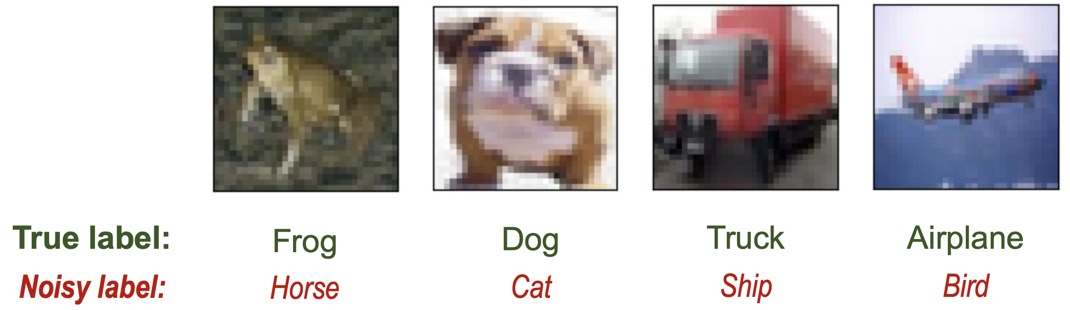
(a) Factual noise

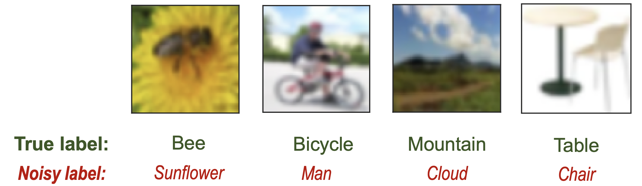
(b) ambiguous noise

Figure 1: Examples of the two noise types in real-world annotation scenarios.

To answer the question, in this paper, we propose a novel sample selection-based method, called Proto-semi, for noisy label learning in real-world annotation scenarios. Similar to previous sample selection-based methods (Garg et al. 2023; Song et al. 2020; Wei et al. 2022b), We first perform a warm-up pretraining to divide the training samples into confident and unconfident datasets. Then we create a prototype vector for each class based on the corresponding samples in the confident dataset, and calculate the distance between each sample in the unconfident dataset and these prototypes. After that, the noise types of samples in the unconfident dataset are identified based on the calculated distance: 1) For samples with a small distance, we consider them to be factual noise and perform label correction. 2) For samples with a distance that is neither too large nor too small, we categorize it as an ambiguous error and correct or retain the label based on the probability according to the distance value. The corrected or retained data, along with their labels, are moved to the confident dataset. Finally, we introduce the semi-supervised learning method (Berthelot et al. 2019) to train the model based on the refined confident and unconfident datasets. In summary, our contributions are followed as:

• We present a new noise-type perspective on noisy label learning in real-world scenarios.

• We propose a novel sample selection-based method called Proto-semi for noisy label learning. Proto-semi introduces prototypes to repartition confident and unconfident datasets based on the types of noise.

• Experiments on the CIFAR-N (Wei et al. 2022b) dataset demonstrate the effectiveness of Proto-semi for noisy label learning in real-world scenarios. Additionally, we use prototype visualization and detailed statistical analysis to confirm that Proto-semi can effectively identify the type of noise and correct the labels for factual noise.

Related Works

Learning From Noisy Labels

The existing literature on noisy label learning can be broadly classified into four categories. The first category focuses on designing more robust architectures, such as dedicated architectures (Xiao et al. 2015; Yao et al. 2019) and the addition of noise adaptation layers (Chen and Gupta 2015; Goldberger and Ben-Reuven 2017) at the top of the softmax layer to model the noise transition matrix. The second category centers on robust regularization, including explicit (Hendrycks, Lee, and Mazeika 2019; Tanno et al. 2019) and implicit regularization (Goodfellow, Shlens, and Szegedy 2015; Lukasik et al. 2020), both of which aim to prevent overfitting in noisy data. The third category focuses on developing more robust loss functions, such as loss regularization (Lyu and Tsang 2020), loss correction (Patrini et al. 2017), and loss reweighing (Liu and Tao 2016). Finally, the last category is sample selection-based (Bai et al. 2021; Li, Socher, and Hoi 2020), which involves selecting true labeled examples from noisy training datasets and has been shown to be the most effective method among all categories.

Sample selection-based methods can be further classified into two categories: loss-based sampling (Sachdeva et al. 2021; Zheltonozhskii et al. 2022) and feature-based sampling (Kim et al. 2021; Wu et al. 2020). Loss-based sample selection methods are based on the small loss hypothesis, which assumes that noisy data tends to incur a high loss due to the model’s inability to accurately classify such data. Feature-based sampling methods distinguish clean and noisy samples by leveraging features. However, both of these categories simply categorize all predicted noisy samples as unlabeled, which does not fully exploit the training data. Therefore, in this paper, we propose a novel noise-type-based sample selection method to enhance the utilization of annotation information in training data.

Prototype Neural Networks

Prototype-based metric learning methods (Snell, Swersky, and Zemel 2017) have emerged as a promising technique in numerous research domains, including few-shot learning (Wang et al. 2021) and meta-learning (Vilalta and Drissi 2002). ProtoNet (Snell, Swersky, and Zemel 2017), which introduces prototypes into deep learning, is a seminal work in this area. Subsequent studies (Li et al. 2021a, b) have focused on improving prototype estimation to enhance classification performance. The success of prototype-based models suggests that prototypes can serve as representative embeddings of instances from the same classes, thereby inspiring us to explore the use of prototype networks in the context of noisy label learning.

Problem Definition

In practical problems, it is often difficult to obtain samples from the true distribution $D$ of a pair of random variables $(\bm{X},\bm{Y})\in\mathcal{X}\times\{1,…K\}$ due to random label corruption. Here, $\bm{X}$ is the sample variable, $\bm{Y}$ is the label variable, $\mathcal{X}$ represents the feature space, and $K$ is the number of classes. Instead, in the context of noisy label learning, we can only access a set of samples $\{{({\bm{x}_{i},\tilde{y}_{i}})_{i=1}^{n}}\}$ that are independently drawn from the distribution $\tilde{D}$ of noisy samples $(\bm{X},\bm{\tilde{Y}})$, where $\bm{\tilde{Y}}$ represents the noisy label variable. The objective is to learn a robust classifier based on noisy samples that can accurately classify test samples.

Method

In this section, we introduce our proposed method Proto-semi for learning with noisy labels in real-world annotation scenarios. Proto-semi is mainly composed of two steps: sample selection and semi-supervised learning. Sample selection is used to divide the whole dataset into the confident and unconfident datasets, in which we propose a prototype-based repartitioning strategy to identify the types of noise and correct their labels. And then semi-supervised learning is introduced to enhance the training based on the repartitioned confident and unconfident datasets. Details of the two steps are described in the following.

Sample Selection

Similar to previous label-noise learning methods based on sample selection (Garg et al. 2023; Song et al. 2020; Wei et al. 2022b), we begin by dividing the original noisy dataset $\{({\bm{x}_{i},\tilde{y}_{i}})_{i=1}^{n}\}$ into two distinct subsets: a labeled confident dataset $\mathcal{D}_{l}$ and an unlabeled unconfident dataset $\mathcal{D}_{u}$. In this work, we accomplish this through a warm-up phase, during which we optimize a training function as follows:

$$\min_{\Theta}\frac{1}{n}\sum_{i=1}^{n}\mathcal{L}(f(\bm{x}_{i};\Theta),{\tilde{y}_{i}}),$$ (1)

where $f(\cdot;\Theta)$ denotes the classifier, such as deep neural networks, $\Theta$ is the parameters of classifier, and $\mathcal{L(\cdot)}$ is the cross-entropy loss function. To avoid the memorization phenomenon (Arpit et al. 2017), we only perform a small number of epochs in the warm-up phase. Upon completing the warm-up phase, we proceed to identify samples across all examples whose classifier soft outputs are consistent with their current labels. The identified samples are put into the confident dataset $\mathcal{D}_{l}$ and their labels are retained. In contrast, samples whose soft outputs and current labels are inconsistent are dropped into unconfident dataset $\mathcal{D}_{u}$ and their labels are discarded. In short, the split process can be summarized by the following two formulas:

$$\mathcal{D}_{l}= \{({\bm{x}_{i},\tilde{y}_{i}})|\tilde{y}_{i}=\hat{y}_{i},i=1,\cdots,n\},$$ (2)

$$\mathcal{D}_{u}= \{\bm{x}_{i}|\tilde{y}_{i}\neq\hat{y}_{i},i=1,\cdots,n\},$$ (3)

where $\hat{y}_{i}$ represents the soft output of classifier $f(\cdot;\Theta)$ on sample $i$. As pointed out by previous works (Bai et al. 2021), during the warm-up phase, the model gradually converges to clean samples that make up the majority of all samples. Therefore, based on the warm-up dividing, the majority of clean samples and noisy samples are assigned to the confident dataset $\mathcal{D}_{l}$ and unconfident dataset $\mathcal{D}_{u}$, respectively. However, as aforementioned in the Introduction, noise in the human annotation scenario can be mainly divided into factual noise and ambiguous noise. To distinguish these noises and utilize the information effectively, we propose a prototype-based repartitioning strategy.

First, we construct an $M$-dimensional representation $\bm{c}_{k}\in\mathcal{R}^{M}$, or prototype, of each class through an embedding function. In this paper, we use the classifier after warm-up and remove its last linear layer as the embedding function, tagged as $f^{{}^{\prime}}(\cdot;\Theta)$. And each prototype is the mean vector of all sample embeddings belonging to its class:

$$\bm{c}_{k} =\frac{1}{|D_{l}^{k}|}\sum_{(\bm{x}_{i},\hat{y}_{i})\in D_{l}^{k}}f^{{}^{\prime}}(\bm{x}_{i};\Theta),$$ (4)

where $D_{l}^{k}$ denotes the all samples that belong to the class $k$ in the confident dataset $D_{l}$, and $|D_{l}^{k}|$ is the number of samples in $D_{l}^{k}$. Similarly, we can obtain the prototype vectors of classes in addition to the class $k$ based on Eq. (4). And we aggregate all the prototype vectors of each class together to obtain the prototype matrix $\mathbf{C}$.

After that, for each sample $u$ in the unconfident dataset $D_{u}$, we calculate the distance between the sample and all prototypes:

$$\bm{d} =Distance(f^{{}^{\prime}}(u;\Theta),\mathbf{C}),$$ (5)

where $\bm{d}$ denotes the distance vector and $Distance(\cdot,\cdot)$ represents the distance function. We use cosine similarity as the distance function in this paper.

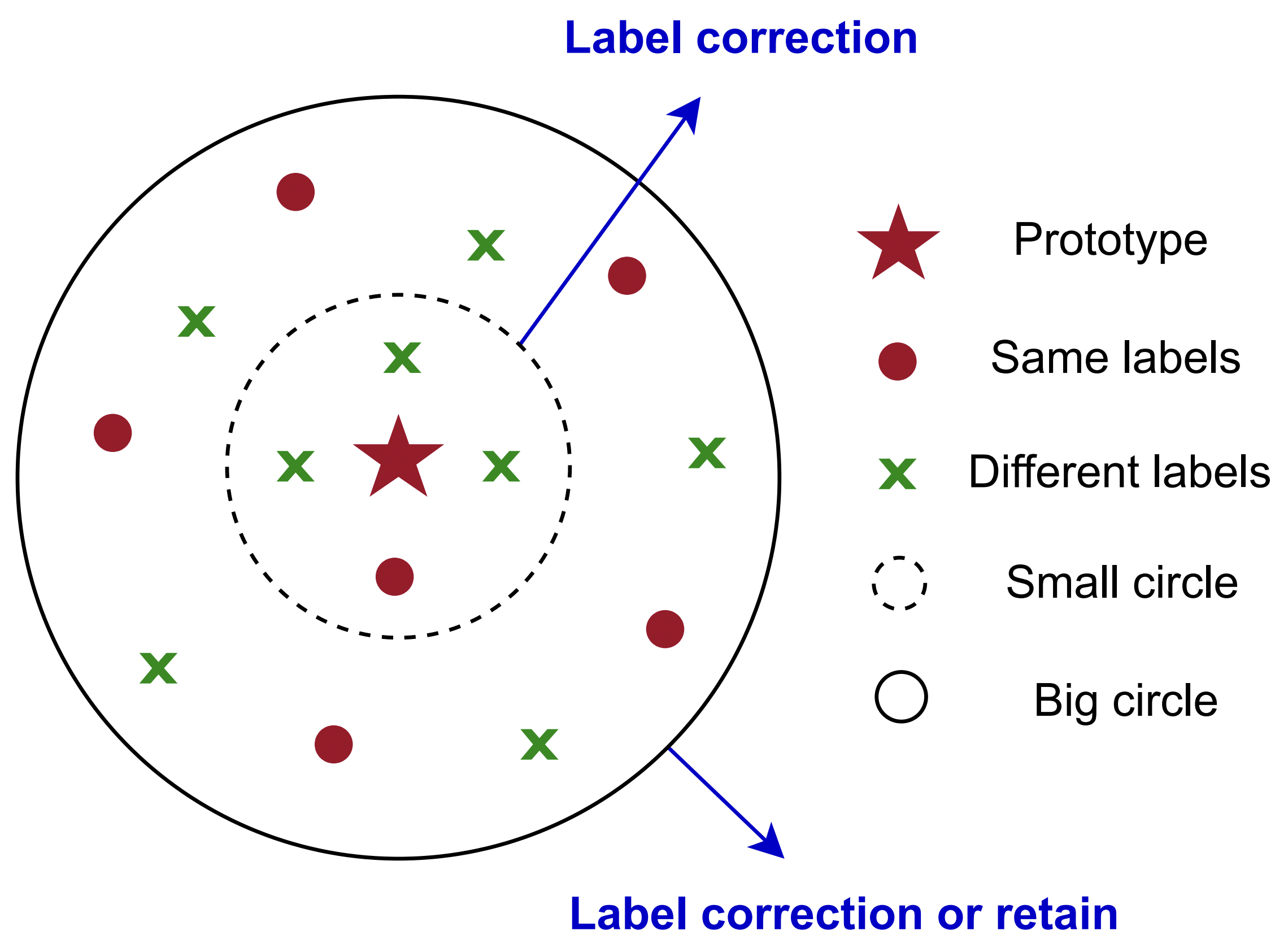
Figure 2: Noise type identifying in Proto-semi.

Then we select the maximum distance $d_{max}$ from the distance vector $\bm{d}$ and assign the class with the highest value as the proto-label . Note that each sample in the unconfident dataset also has its original label, referred to as the noisy-label. Based on the prototype of the proto-label, two circles are constructed as shown in the Figure 2: 1) Small circle: the distance to the prototype is less than the lower threshold $\alpha$. 2) Big circle: the distance to the prototype is less than the upper threshold $\beta$. Based on the two circles, we are able to determine which samples should be moved from the unconfident dataset $D_{u}$ to the confident dataset $D_{l}$:

• The sample that fall within the small circle ($d_{max}<\alpha$): The sample will be assigned the proto-label. If the noisy-label is different from the proto-label, this indicates the factual noise is identified and corrected.

• The samples that lie between the small and big circles ( $\alpha\leq d_{max}<\beta$): If the noisy-label is equal to the proto-label, the sample’s original label, namely noisy-label, will be retained; Otherwise, the sample will be corrected to the proto-label probabilistically based on the distance to the prototype, with the probability of correction increasing as the distance decreases. This randomness allows us to correct factual noises while also utilizing semantic information from ambiguous noises.

Finally, all unconfident samples that fall within the big circle (including the small circle), after label correction or retention, will be moved to the confident dataset, creating new confident and unconfident datasets.

Semi-supervised Learning

After the new confident dataset $D_{l}$ and unconfident dataset $D_{u}$ are generated, inspired by the previous noisy label learning works (Garg et al. 2023; Song et al. 2020; Wei et al. 2022b), we introduce the semi-supervised training method, MixMatch (Berthelot et al. 2019), to enhance the training in Proto-semi. The procedure of semi-supervised learning used in Proto-semi is as follows.

We begin by augmenting the data in both the refinement confident dataset $D_{l}$ and the unconfident dataset $D_{u}$, resulting in the new augmented datasets $D_{l}^{{}^{\prime}}$ and $D_{u}^{{}^{\prime}}$, respectively. Following the approach described in (Bai et al. 2021), we apply the augmentation technique with two different strategies to each dataset:

$$D_{l1}^{{}^{\prime}} =\text{{Augment}}_{1}(D_{l}),D_{l2}^{{}^{\prime}}=\text{{Augment}}_{2}(D_{l}),$$ (6)

$$D_{u1}^{{}^{\prime}} =\text{{Augment}}_{1}(D_{u}),D_{u2}^{{}^{\prime}}=\text{{Augment}}_{2}(D_{u}),$$ (7)

where Augment_(⋅) denotes the augmentation technique.

Particularly, we use the aggregated model soft outputs of $D_{u1}^{{}^{\prime}}$ and $D_{u2}^{{}^{\prime}}$ to guess the pseudo-labels for the augmented unconfident dataset. After that, Mixup (Zhang et al. 2018) is incorporated to combine the inputs and labels in two confident datasets ($D_{l1}^{{}^{\prime}}$, $D_{l2}^{{}^{\prime}}$) and unconfident datasets ($D_{u1}^{{}^{\prime}}$, $D_{u2}^{{}^{\prime}}$), respectively. Finally, for the combined confident dataset, we use the cross-entropy loss $\mathcal{L}_{l}$ to evaluate the difference between the outputs and true labels. While for the combined unconfident dataset, the L2 loss $\mathcal{L}_{u}$ is introduced to evaluate the discrepancy between the outputs and pseudo-labels. And the final training loss is the weighted sum of the two losses:

$$\mathcal{L}_{final} =\mathcal{L}_{l}+\lambda\mathcal{L}_{u},$$ (8)

where $\lambda$ is the balance factor.

We summarize the overall procedure of Proto-semi in Algorithm 1.

Input: Neural network with trainable parameters $\Theta$, Noisy training dataset $\{(\bm{x}_{i},\tilde{y}_{i})\}_{i=1}^{n}$, Number of warm-up epochs $T_{w}$, proto split epochs $T_{p}$, and training epochs $T_{t}$ for refining with confident examples and unconfident examples, Lower threshold $\alpha$, Upper threshold $\beta$.

for $i=1,\dots,T_{w}$  do

       Optimize network parameter $\Theta$ with Eq. (1);

      

for $i=1,\dots,T_{c}$  do

      

      Extract confident example set $\mathcal{D}_{l}$ and unlabeled set $\mathcal{D}_{u}$ based on classifier $f(\cdot,\Theta)$ with Eq. (2) and Eq. (3);

       if $i<T_{p}$ then

             Contruct prototype for each class based on $\mathcal{D}_{l}$ with Eq. (4);

             for $u\in\mathcal{D}_{u}$ do

                   Calculate the distances between $u$ and all class prototypes with Eq. (5);

                   Select the maximum value $d_{max}$ in all distances;

                   if $d_{max}\leq\alpha$ then

                         Assign the class corresponding to $d_{max}$ as the label of $u$;

                         Move $u$ from $\mathcal{D}_{u}$ to $\mathcal{D}_{l}$;

                        

                  if $d_{max}>\alpha\And d_{max}\leq\beta$ then

                         Assign the class corresponding to $d_{max}$ as the label of $u$ or retain the original label of $u$ with regard to the value of $d_{max}$;

                         Move $u$ from $\mathcal{D}_{u}$ to $\mathcal{D}_{l}$ ;

                        

                  

            

      Training the classifier $f(\cdot,\Theta)$ with MixMatch loss on the new generated $\mathcal{D}_{l}$ and $\mathcal{D}_{u}$ with Eq. (8);

 

Evaluate the obtained classifier $f(\cdot,\Theta)$.

Algorithm 1 The Overall Procedure of Proto-semi

Experiments

Table 1: The classification results (%) over the methods on the CIFAR-N dataset w.r.t. accuracy. We highlight the best results in bold and the runner-up results with underline.

Methods	CIFAR-10N					CIFAR-100N
	aggre	rand1	rand2	rand3	worst	noisy
Co-Teaching	91.20$\pm$0.13	90.33$\pm$0.13	90.30$\pm$0.17	90.15$\pm$0.18	83.83$\pm$0.13	60.37$\pm$0.27
Peer-Loss	90.75$\pm$0.25	89.06$\pm$0.11	88.76$\pm$0.19	88.57$\pm$0.09	82.53$\pm$0.52	57.59$\pm$0.61
Divide-Mix	95.01$\pm$0.71	95.16$\pm$0.19	95.23$\pm$0.07	95.21$\pm$0.14	92.56$\pm$0.42	$\mathbf{71.13\pm 0.48}$
ELR	92.38$\pm$0.64	91.46$\pm$0.38	91.61$\pm$0.16	91.41$\pm$0.44	83.58$\pm$0.13	58.94$\pm$0.92
ELR+	94.83$\pm$0.10	94.43$\pm$0.41	94.20$\pm$0.24	94.34$\pm$0.22	91.09$\pm$1.60	66.72$\pm$0.07
Positive-LS	91.57$\pm$0.07	89.80$\pm$0.28	89.35$\pm$0.33	89.82$\pm$0.14	82.76$\pm$0.53	55.84$\pm$0.48
PES-semi	94.66$\pm$0.18	95.06$\pm$0.15	95.19$\pm$0.23	95.22$\pm$0.13	92.68$\pm$0.22	70.36$\pm$0.33
CAL	91.97$\pm$0.32	90.93$\pm$0.31	90.75$\pm$0.30	90.74$\pm$0.22	85.36$\pm$0.16	61.73$\pm$0.42
CORES	91.23$\pm$0.11	89.66$\pm$0.32	89.91$\pm$0.45	89.79$\pm$0.50	83.60$\pm$0.53	61.15$\pm$0.73
CORES∗	95.25$\pm$0.09	94.45$\pm$0.14	94.88$\pm$0.31	94.74$\pm$0.03	91.66$\pm$1.60	55.72$\pm$0.42
CE	87.77$\pm$0.38	85.02$\pm$0.65	86.46$\pm$1.79	85.16$\pm$0.61	77.69$\pm$1.55	55.50$\pm$0.66
Negative-LS	91.97$\pm$0.32	90.29$\pm$0.32	90.37$\pm$0.12	90.13$\pm$0.19	82.99$\pm$0.36	58.59$\pm$0.98
SOP	$\mathbf{95.61\pm 0.13}$	95.28$\pm$0.13	95.31$\pm$0.10	95.39$\pm$0.11	$\mathbf{93.24\pm 0.21}$	67.81$\pm$0.23
Proto-semi (Best)	95.03$\pm$0.14	$\mathbf{95.48\pm 0.17}$	$\mathbf{95.48\pm 0.21}$	$\mathbf{95.67\pm 0.10}$	92.97$\pm$0.33	67.73$\pm$0.67
Proto-semi (Last)	94.82$\pm$0.15	95.40$\pm$0.21	95.37$\pm$0.33	95.53$\pm$0.09	92.48$\pm$0.18	67.44$\pm$0.22

In this section, we evaluate the performance of Proto-semi by comparing it with representative noisy label learning methods on the datasets that are generated from real-world annotation scenarios.

Dataset

Table 2: The statistics of CIFAR-N dataset

Dataset	Subset	Train/Test size	Classes	Noise rate
CIFAR-10N	aggre	50K/10K	10	9.03%
	rand1	50K/10K	10	$\approx$18%
	rand2	50K/10K	10	$\approx$18%
	rand3	50K/10K	10	$\approx$18%
	worst	50K/10K	10	40.21%
CIFAR-100N	noisy	50K/10K	100	40.20%

Following previous works (Liu et al. 2022), we use the CIFAR-N (Wei et al. 2022b) dataset as the experimental benchmark, which has six subsets. CIFAR-N is created by relabeling CIFAR-10N/CIFAR-100N with Amazon Mechanical Turk labeling of the original CIFAR-10/CIFAR-100 dataset (Krizhevsky, Hinton et al. 2009). The CIFAR-10N dataset contains five distinct noise rate options, including aggre, rand1, rand2, rand3, and worst. While the CIFAR-100N dataset only has one noise rate, namely noisy. Table 2 gives the statistics of all subsets in the CIFAR-N.

Baselines

We choose the representative noisy label learning methods as the comparison methods:

• Co-Teaching (Han et al. 2018) trains two neural networks simultaneously and lets them teach each other.

• Peer-Loss (Liu and Guo 2020) introduces a new family of loss functions based on the standard empirical risk minimization framework.

• Divide-Mix (Li, Socher, and Hoi 2020) models the per-sample loss distribution to perform sample selection and improves MixMatch.

• ELR (Liu et al. 2020) designs a regularization term to prevent memorization of the false labels. And ELR+ (Liu et al. 2020) introduces cosine annealing learning rate to enhance training based on ELR.

• Positive-LS (Lukasik et al. 2020) introduces label smoothing and shows its effect is similar to label correction.

• PES-semi (Bai et al. 2021) separates the neural networks into different parts and progressively trains them.

• CAL (Zhu, Liu, and Liu 2021) proposes a new loss function based on covariance-assisted learning.

• CORES (Cheng et al. 2021) progressively sieves out corrupted examples from instance-dependent label noise. And CORES^∗ (Cheng et al. 2021) applies consistency training.

• CE (Wei et al. 2022b) constructs the CIFAR-N dataset and performs the base cross-entropy model.

• Negative-LS (Wei et al. 2022a) proposes a negative weight to combine the hard and soft labels.

• SOP (Liu et al. 2022) proposes a principled approach for robust training of over-parameterized deep networks.

Implementation details

We implement Proto-semi by PyTorch. For fairness, all experiments are performed on a single 1080Ti GPU. We use the ResNet34 (He et al. 2016) as the backbone and optimize it by SGD with cosine scheduler. For each dataset, we run 5 times and report the mean and standard deviation. The learning rate, training epoch and weight decay are set to 0.02, 600, and 0.0005, respectively. And we perform a grid search to tune hyper-parameters: warm-up epoch $T_{w}\in\{10,20,30\}$, proto split epoch $T_{p}\in\{1,2,3\}$, lower threshold $\alpha\in\{0.99,0.97,0.95\}$, upper threshold $\beta\in\{0.94,0.92,0.90\}$. In semi-supervised learning, we apply random crop and flip to perform augmentation on the photos of CIFAR-N. The temperature for Mixup is set to $0.5$, and the balance factor $\lambda$ follows a linear decay value from the warm-up epoch to the training epoch.

Experimental results

Table 1 shows the evaluation results on the CIFAR-N dataset. We take the results of other baselines from the leaderboard  of CIFAR-N. From the table, we observe: 1) Proto-semi achieves the best average performance on all CIFAR-N datasets. Notably, Proto-semi has surpassed the state-of-the-art (SOTA) results on the rand1, rand2, and rand3 datasets. This demonstrates the effectiveness of our approach for addressing the noisy label learning problem in real annotation scenarios. 2) Proto-semi performs better on datasets with fewer classes, namely CIFAR-10N, as it can effectively construct prototype vectors for each category on these datasets. Oppositely, the generated class-prototype vectors on datasets with more categories (CIFAR-100N) are difficult to distinguish. We will discuss this phenomenon in the further experiments (See the last two experiments). 3) Sample selection-based methods, including Divide-Mix, PES-semi, and our proposed method Proto-semi all achieve relatively high performance, highlighting the importance of dividing the noisy dataset into confident dataset and unconfident dataset in noisy label learning.

Ablation Study

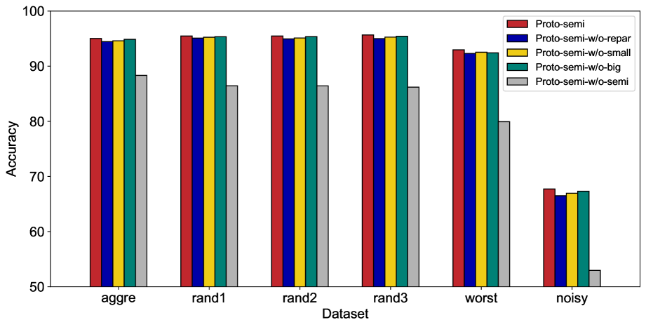
Figure 3: Ablation study on Proto-semi. From left to right: Proto-semi, Proto-semi-w/o-repar, Proto-semi-w/o-small, Proto-semi-w/o-big, Proto-semi-w/o-semi.

We further conduct ablation study to verify the importance of its main components in Proto-semi, including the repartitioning strategy in the sample selection, and the semi-supervised learning. As shown in Figure 3, we implement four variants of Proto-semi by removing the corresponding component.

We name the first variant Proto-semi-w/o-repar, which removes the repartitioning strategy in the sample selection. As in Figure 3, we observe declines in performance across all datasets. This suggests that our proposed repartitioning strategy can generate better confident and unconfident datasets, which ultimately helps Proto-semi achieve better classification performance. To further validate the impact of the re-partitioning strategy in detail, we conduct two ablation analyses and introduce two new variants: Proto-semi-w/o-small and Proto-semi-w/o-big. The former involves removing the construction of the small circle in the re-partitioning strategy, which means that we do not identify factual noise. On the other hand, the latter omits the construction of the large circle in the re-partitioning process, resulting in the failure to identify ambiguous noise. The results in Figure 3 show that removing either circle construction leads to a decrease in the model’s final performance compared to the complete method, indicating that both circle constructions are essential for the sample re-partitioning strategy. Moreover, on most datasets, removing the small circle construction has a greater impact on performance reduction than removing the large circle construction. This suggests that constructing small circles can effectively identify factual noises and correct their labels. Notably, on the CIFAR-10(worst) dataset, retaining ambiguous noise can improve the model’s robustness and performance to some extent compared to removing the strategy that constructs small circles. The last variant, Proto-semi-w/o-semi, involves discarding the semi-supervised learning step and retaining only the warmup stage described in Algorithm 1. Figure 3 shows a significant drop in performance across all datasets with this variant. Furthermore, Table 1 demonstrates that methods based on semi-supervised learning, such as PES-semi (Bai et al. 2021) and Divide-Mix (Li, Socher, and Hoi 2020), perform well on the CIFAR-N dataset. These findings indicate that the training augmentation provided by semi-supervised learning is highly effective for the noisy label learning in real-world annotation scenarios.

Prototype Embedding Visualization

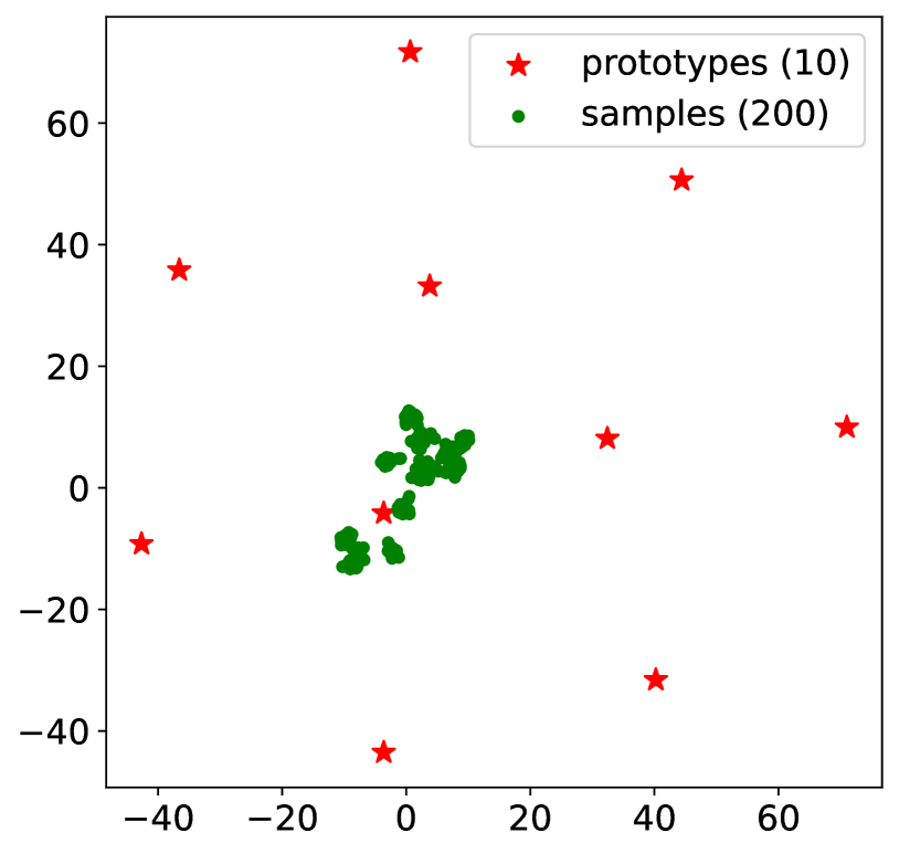
(a) CIFAR-10N (rand2)

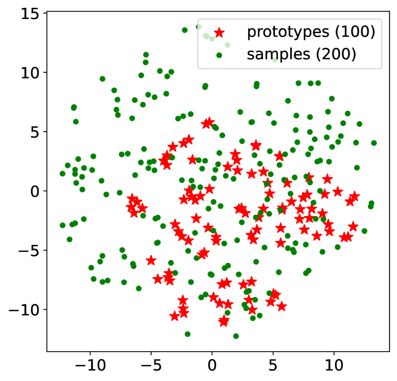
(b) CIFAR-100N (noisy)

Figure 4: Visualization of prototype embedding on the CIFAR-N dataset.

Table 3: The label correction results of small circle in Proto-semi ($T_{w}=20,\alpha=0.95$).

	CIFAR-10N					CIFAR-100N
	aggre	rand1	rand2	rand3	worst	noisy
Size of unconfident dataset	10534	10995	10611	5836	21946	25096
Number of samples in small circle	4015	5766	4258	1729	9472	1823
Number of label corrections:	3992	5703	4235	1713	9381	1708
Right Number of label corrections	3846	5416	4097	1666	8723	1325
Correction accuracy	96.34%	94.97%	96.74%	97.26%	92.99%	77.58%

To validate the effectiveness of prototype vector construction and its performance on learning with noisy labels, we conduct dimensionality reduction and visualization experiments using t-SNE. We choose CIFAR-10N (rand2) and CIFAR-100N (noisy) as the experimental datasets. Then a batch of 200 samples are randomly extracted from the unconfident dataset and perform visualization with all class prototype vectors. The visualization results are shown in Figure 4. Figure 4a depicts the visualization result on the CIFAR-10N (rand2) dataset. It can be observed that the 10 class prototype vectors were evenly distributed in the two-dimensional space, and the 200 sample vectors were effectively clustered around a class prototype vector. This facilitated label correction or retention based on distance. While Figure 4b shows the visualization result for the CIFAR-100N (noisy) dataset where the 100 class prototype vectors and 200 sample vectors were scattered without any discernible patterns in the two-dimensional space. Some prototype vectors even overlap, making it challenging to reassign the samples based on these class prototype vectors. Despite using high thresholds, we found it difficult to classify these samples in our CIFAR-100N experiment.

Overall, the visualization results in Figure 4 indicate that our prototype-based repartitioning strategy can effectively learn class information in the dataset with few classes. By reassigning samples based on distances and correcting their labels, this strategy helps Proto-semi achieve good results in learning with label noise.

Label Correction Analysis

In the last experiment, we analyze the effectiveness of the proposed prototype-based repartitioning strategy in correcting labels. We record several metrics, including the size of the unconfident dataset, the number of samples falling within a small circle (See Figure 1), the number of samples corrected within the small circle, the number of samples correctly corrected, and the accuracy of correct corrections on all CIFAR-N datasets after the warm-up phase. The results are presented in Table 3, and the following discoveries can be drawn: 1) The strategy is highly effective in correcting labels. The accuracy of correction is higher than the model’s final predictive performance on almost all datasets (See Table 1). Remarkably, the strategy achieves an impressive 97.26% accuracy on the CIFAR-10N (rand3) dataset. 2) The majority of samples falling within the small circle require label correction due to factual noise. For instance, the CIFAR-10N (rand1) dataset and the CIFAR-100N (noisy) dataset have 5766 and 1823 samples within the small circle, respectively, with 5416 and 1708 samples needing correction. 3) The strategy performs better on datasets with fewer classes. This is shown by the lower number of unreliable samples, more samples within the small circle, and greater accuracy in label correction for all CIFAR-10N datasets compared to CIFAR-100N. These findings are consistent with the results presented in Figure 4.

Conclusion

In this paper, we present a novel sample selection-based approach, denoted as Proto-semi, for effectively identifying the type of noise and utilizing its semantics in real-world annotation scenarios. Specifically, Proto-semi divides the entire dataset into two subsets, namely confident and unconfident datasets, and subsequently leverages a distance-based technique based on prototype vectors to identify the types of annotation noise. Furthermore, the confident and unconfident datasets are adjusted based on the distances, and a semi-supervised learning strategy is incorporated to enhance the training process. Experimental results on the CIFAR-N dataset demonstrate the effectiveness of Proto-semi in addressing the problem of learning with noisy labels in real-world annotation scenarios. Avenue of future work will focus on extending our proposed method to more real-world annotation noisy datasets.

References

- Arazo et al. (2019) Arazo, E.; Ortego, D.; Albert, P.; O’Connor, N. E.; and McGuinness, K. 2019. Unsupervised Label Noise Modeling and Loss Correction. In Chaudhuri, K.; and Salakhutdinov, R., eds., Proceedings of the 36th International Conference on Machine Learning, ICML 2019, 9-15 June 2019, Long Beach, California, USA, volume 97 of Proceedings of Machine Learning Research, 312–321. PMLR.
- Arpit et al. (2017) Arpit, D.; Jastrzebski, S.; Ballas, N.; Krueger, D.; Bengio, E.; Kanwal, M. S.; Maharaj, T.; Fischer, A.; Courville, A. C.; Bengio, Y.; and Lacoste-Julien, S. 2017. A Closer Look at Memorization in Deep Networks. In Precup, D.; and Teh, Y. W., eds., Proceedings of the 34th International Conference on Machine Learning, ICML 2017, Sydney, NSW, Australia, 6-11 August 2017, volume 70 of Proceedings of Machine Learning Research, 233–242. PMLR.
- Bai et al. (2021) Bai, Y.; Yang, E.; Han, B.; Yang, Y.; Li, J.; Mao, Y.; Niu, G.; and Liu, T. 2021. Understanding and Improving Early Stopping for Learning with Noisy Labels. In Ranzato, M.; Beygelzimer, A.; Dauphin, Y. N.; Liang, P.; and Vaughan, J. W., eds., Advances in Neural Information Processing Systems 34: Annual Conference on Neural Information Processing Systems 2021, NeurIPS 2021, December 6-14, 2021, virtual, 24392–24403.
- Berthelot et al. (2019) Berthelot, D.; Carlini, N.; Goodfellow, I. J.; Papernot, N.; Oliver, A.; and Raffel, C. 2019. MixMatch: A Holistic Approach to Semi-Supervised Learning. In Wallach, H. M.; Larochelle, H.; Beygelzimer, A.; d’Alché-Buc, F.; Fox, E. B.; and Garnett, R., eds., Advances in Neural Information Processing Systems 32: Annual Conference on Neural Information Processing Systems 2019, NeurIPS 2019, December 8-14, 2019, Vancouver, BC, Canada, 5050–5060.
- Chen and Gupta (2015) Chen, X.; and Gupta, A. 2015. Webly Supervised Learning of Convolutional Networks. In 2015 IEEE International Conference on Computer Vision, ICCV 2015, Santiago, Chile, December 7-13, 2015, 1431–1439. IEEE Computer Society.
- Cheng et al. (2021) Cheng, H.; Zhu, Z.; Li, X.; Gong, Y.; Sun, X.; and Liu, Y. 2021. Learning with Instance-Dependent Label Noise: A Sample Sieve Approach. In 9th International Conference on Learning Representations, ICLR 2021, Virtual Event, Austria, May 3-7, 2021. OpenReview.net.
- Doan, Ramakrishnan, and Halevy (2011) Doan, A.; Ramakrishnan, R.; and Halevy, A. Y. 2011. Crowdsourcing systems on the World-Wide Web. Commun. ACM, 54(4): 86–96.
- Garg et al. (2023) Garg, A.; Nguyen, C.; Felix, R.; Do, T.; and Carneiro, G. 2023. PASS: Peer-Agreement based Sample Selection for training with Noisy Labels. CoRR, abs/2303.10802.
- Goldberger and Ben-Reuven (2017) Goldberger, J.; and Ben-Reuven, E. 2017. Training deep neural-networks using a noise adaptation layer. In 5th International Conference on Learning Representations, ICLR 2017, Toulon, France, April 24-26, 2017, Conference Track Proceedings. OpenReview.net.
- Goodfellow, Shlens, and Szegedy (2015) Goodfellow, I. J.; Shlens, J.; and Szegedy, C. 2015. Explaining and Harnessing Adversarial Examples. In Bengio, Y.; and LeCun, Y., eds., 3rd International Conference on Learning Representations, ICLR 2015, San Diego, CA, USA, May 7-9, 2015, Conference Track Proceedings.
- Han et al. (2018) Han, B.; Yao, Q.; Yu, X.; Niu, G.; Xu, M.; Hu, W.; Tsang, I. W.; and Sugiyama, M. 2018. Co-teaching: Robust training of deep neural networks with extremely noisy labels. In Bengio, S.; Wallach, H. M.; Larochelle, H.; Grauman, K.; Cesa-Bianchi, N.; and Garnett, R., eds., Advances in Neural Information Processing Systems 31: Annual Conference on Neural Information Processing Systems 2018, NeurIPS 2018, December 3-8, 2018, Montréal, Canada, 8536–8546.
- He et al. (2016) He, K.; Zhang, X.; Ren, S.; and Sun, J. 2016. Deep Residual Learning for Image Recognition. In 2016 IEEE Conference on Computer Vision and Pattern Recognition, CVPR 2016, Las Vegas, NV, USA, June 27-30, 2016, 770–778. IEEE Computer Society.
- Hendrycks, Lee, and Mazeika (2019) Hendrycks, D.; Lee, K.; and Mazeika, M. 2019. Using Pre-Training Can Improve Model Robustness and Uncertainty. In Chaudhuri, K.; and Salakhutdinov, R., eds., Proceedings of the 36th International Conference on Machine Learning, ICML 2019, 9-15 June 2019, Long Beach, California, USA, volume 97 of Proceedings of Machine Learning Research, 2712–2721. PMLR.
- Jindal, Nokleby, and Chen (2016) Jindal, I.; Nokleby, M. S.; and Chen, X. 2016. Learning Deep Networks from Noisy Labels with Dropout Regularization. In Bonchi, F.; Domingo-Ferrer, J.; Baeza-Yates, R.; Zhou, Z.; and Wu, X., eds., IEEE 16th International Conference on Data Mining, ICDM 2016, December 12-15, 2016, Barcelona, Spain, 967–972. IEEE Computer Society.
- Kim et al. (2021) Kim, T.; Ko, J.; Cho, S.; Choi, J.; and Yun, S. 2021. FINE Samples for Learning with Noisy Labels. In Ranzato, M.; Beygelzimer, A.; Dauphin, Y. N.; Liang, P.; and Vaughan, J. W., eds., Advances in Neural Information Processing Systems 34: Annual Conference on Neural Information Processing Systems 2021, NeurIPS 2021, December 6-14, 2021, virtual, 24137–24149.
- Krizhevsky, Hinton et al. (2009) Krizhevsky, A.; Hinton, G.; et al. 2009. Learning multiple layers of features from tiny images.
- Li et al. (2021a) Li, G.; Jampani, V.; Sevilla-Lara, L.; Sun, D.; Kim, J.; and Kim, J. 2021a. Adaptive Prototype Learning and Allocation for Few-Shot Segmentation. In IEEE Conference on Computer Vision and Pattern Recognition, CVPR 2021, virtual, June 19-25, 2021, 8334–8343. Computer Vision Foundation / IEEE.
- Li, Socher, and Hoi (2020) Li, J.; Socher, R.; and Hoi, S. C. H. 2020. DivideMix: Learning with Noisy Labels as Semi-supervised Learning. In 8th International Conference on Learning Representations, ICLR 2020, Addis Ababa, Ethiopia, April 26-30, 2020. OpenReview.net.
- Li et al. (2021b) Li, J.; Zhou, P.; Xiong, C.; and Hoi, S. C. H. 2021b. Prototypical Contrastive Learning of Unsupervised Representations. In 9th International Conference on Learning Representations, ICLR 2021, Virtual Event, Austria, May 3-7, 2021. OpenReview.net.
- Liu et al. (2020) Liu, S.; Niles-Weed, J.; Razavian, N.; and Fernandez-Granda, C. 2020. Early-Learning Regularization Prevents Memorization of Noisy Labels. In Larochelle, H.; Ranzato, M.; Hadsell, R.; Balcan, M.; and Lin, H., eds., Advances in Neural Information Processing Systems 33: Annual Conference on Neural Information Processing Systems 2020, NeurIPS 2020, December 6-12, 2020, virtual.
- Liu et al. (2022) Liu, S.; Zhu, Z.; Qu, Q.; and You, C. 2022. Robust Training under Label Noise by Over-parameterization. In Chaudhuri, K.; Jegelka, S.; Song, L.; Szepesvári, C.; Niu, G.; and Sabato, S., eds., International Conference on Machine Learning, ICML 2022, 17-23 July 2022, Baltimore, Maryland, USA, volume 162 of Proceedings of Machine Learning Research, 14153–14172. PMLR.
- Liu and Tao (2016) Liu, T.; and Tao, D. 2016. Classification with Noisy Labels by Importance Reweighting. IEEE Trans. Pattern Anal. Mach. Intell., 38(3): 447–461.
- Liu and Guo (2020) Liu, Y.; and Guo, H. 2020. Peer Loss Functions: Learning from Noisy Labels without Knowing Noise Rates. In Proceedings of the 37th International Conference on Machine Learning, ICML 2020, 13-18 July 2020, Virtual Event, volume 119 of Proceedings of Machine Learning Research, 6226–6236. PMLR.
- Lukasik et al. (2020) Lukasik, M.; Bhojanapalli, S.; Menon, A. K.; and Kumar, S. 2020. Does label smoothing mitigate label noise? In Proceedings of the 37th International Conference on Machine Learning, ICML 2020, 13-18 July 2020, Virtual Event, volume 119 of Proceedings of Machine Learning Research, 6448–6458. PMLR.
- Lyu and Tsang (2020) Lyu, Y.; and Tsang, I. W. 2020. Curriculum Loss: Robust Learning and Generalization against Label Corruption. In 8th International Conference on Learning Representations, ICLR 2020, Addis Ababa, Ethiopia, April 26-30, 2020. OpenReview.net.
- Ouyang et al. (2022) Ouyang, L.; Wu, J.; Jiang, X.; Almeida, D.; Wainwright, C. L.; Mishkin, P.; Zhang, C.; Agarwal, S.; Slama, K.; Ray, A.; Schulman, J.; Hilton, J.; Kelton, F.; Miller, L.; Simens, M.; Askell, A.; Welinder, P.; Christiano, P. F.; Leike, J.; and Lowe, R. 2022. Training language models to follow instructions with human feedback. In NeurIPS.
- Patrini et al. (2017) Patrini, G.; Rozza, A.; Menon, A. K.; Nock, R.; and Qu, L. 2017. Making Deep Neural Networks Robust to Label Noise: A Loss Correction Approach. In 2017 IEEE Conference on Computer Vision and Pattern Recognition, CVPR 2017, Honolulu, HI, USA, July 21-26, 2017, 2233–2241. IEEE Computer Society.
- Sachdeva et al. (2021) Sachdeva, R.; Cordeiro, F. R.; Belagiannis, V.; Reid, I. D.; and Carneiro, G. 2021. EvidentialMix: Learning with Combined Open-set and Closed-set Noisy Labels. In IEEE Winter Conference on Applications of Computer Vision, WACV 2021, Waikoloa, HI, USA, January 3-8, 2021, 3606–3614. IEEE.
- Snell, Swersky, and Zemel (2017) Snell, J.; Swersky, K.; and Zemel, R. S. 2017. Prototypical Networks for Few-shot Learning. In Guyon, I.; von Luxburg, U.; Bengio, S.; Wallach, H. M.; Fergus, R.; Vishwanathan, S. V. N.; and Garnett, R., eds., Advances in Neural Information Processing Systems 30: Annual Conference on Neural Information Processing Systems 2017, December 4-9, 2017, Long Beach, CA, USA, 4077–4087.
- Song et al. (2020) Song, H.; Kim, M.; Park, D.; and Lee, J. 2020. Learning from Noisy Labels with Deep Neural Networks: A Survey. CoRR, abs/2007.08199.
- Tanno et al. (2019) Tanno, R.; Saeedi, A.; Sankaranarayanan, S.; Alexander, D. C.; and Silberman, N. 2019. Learning From Noisy Labels by Regularized Estimation of Annotator Confusion. In IEEE Conference on Computer Vision and Pattern Recognition, CVPR 2019, Long Beach, CA, USA, June 16-20, 2019, 11244–11253. Computer Vision Foundation / IEEE.
- Vilalta and Drissi (2002) Vilalta, R.; and Drissi, Y. 2002. A Perspective View and Survey of Meta-Learning. Artif. Intell. Rev., 18(2): 77–95.
- Wang et al. (2021) Wang, Y.; Yao, Q.; Kwok, J. T.; and Ni, L. M. 2021. Generalizing from a Few Examples: A Survey on Few-shot Learning. ACM Comput. Surv., 53(3): 63:1–63:34.
- Wei et al. (2022a) Wei, J.; Liu, H.; Liu, T.; Niu, G.; Sugiyama, M.; and Liu, Y. 2022a. To Smooth or Not? When Label Smoothing Meets Noisy Labels. In Chaudhuri, K.; Jegelka, S.; Song, L.; Szepesvári, C.; Niu, G.; and Sabato, S., eds., International Conference on Machine Learning, ICML 2022, 17-23 July 2022, Baltimore, Maryland, USA, volume 162 of Proceedings of Machine Learning Research, 23589–23614. PMLR.
- Wei et al. (2022b) Wei, J.; Zhu, Z.; Cheng, H.; Liu, T.; Niu, G.; and Liu, Y. 2022b. Learning with Noisy Labels Revisited: A Study Using Real-World Human Annotations. In The Tenth International Conference on Learning Representations, ICLR 2022, Virtual Event, April 25-29, 2022. OpenReview.net.
- Wu et al. (2020) Wu, P.; Zheng, S.; Goswami, M.; Metaxas, D. N.; and Chen, C. 2020. A Topological Filter for Learning with Label Noise. In Larochelle, H.; Ranzato, M.; Hadsell, R.; Balcan, M.; and Lin, H., eds., Advances in Neural Information Processing Systems 33: Annual Conference on Neural Information Processing Systems 2020, NeurIPS 2020, December 6-12, 2020, virtual.
- Xiao et al. (2015) Xiao, T.; Xia, T.; Yang, Y.; Huang, C.; and Wang, X. 2015. Learning from massive noisy labeled data for image classification. In IEEE Conference on Computer Vision and Pattern Recognition, CVPR 2015, Boston, MA, USA, June 7-12, 2015, 2691–2699. IEEE Computer Society.
- Yao et al. (2019) Yao, J.; Wang, J.; Tsang, I. W.; Zhang, Y.; Sun, J.; Zhang, C.; and Zhang, R. 2019. Deep Learning From Noisy Image Labels With Quality Embedding. IEEE Trans. Image Process., 28(4): 1909–1922.
- Zhang et al. (2018) Zhang, H.; Cissé, M.; Dauphin, Y. N.; and Lopez-Paz, D. 2018. mixup: Beyond Empirical Risk Minimization. In 6th International Conference on Learning Representations, ICLR 2018, Vancouver, BC, Canada, April 30 - May 3, 2018, Conference Track Proceedings. OpenReview.net.
- Zheltonozhskii et al. (2022) Zheltonozhskii, E.; Baskin, C.; Mendelson, A.; Bronstein, A. M.; and Litany, O. 2022. Contrast to Divide: Self-Supervised Pre-Training for Learning with Noisy Labels. In IEEE/CVF Winter Conference on Applications of Computer Vision, WACV 2022, Waikoloa, HI, USA, January 3-8, 2022, 387–397. IEEE.
- Zhu, Liu, and Liu (2021) Zhu, Z.; Liu, T.; and Liu, Y. 2021. A Second-Order Approach to Learning With Instance-Dependent Label Noise. In IEEE Conference on Computer Vision and Pattern Recognition, CVPR 2021, virtual, June 19-25, 2021, 10113–10123. Computer Vision Foundation / IEEE.